Submodel Partitioning in Hierarchical
Federated Learning: Algorithm Design and
Convergence Analysis

Abstract

Hierarchical federated learning (HFL) has demonstrated promising scalability advantages over the traditional “star-topology” architecture-based federated learning (FL). However, HFL still imposes significant computation, communication, and storage burdens on the edge, especially when training a large-scale model over resource-constrained Internet of Things (IoT) devices. In this paper, we propose hierarchical independent submodel training (HIST), a new FL methodology that aims to address these issues in hierarchical settings. The key idea behind HIST is a hierarchical version of model partitioning, where we partition the global model into disjoint submodels in each round, and distribute them across different cells, so that each cell is responsible for training only one partition of the full model. This enables each client to save computation/storage costs while alleviating the communication loads throughout the hierarchy. We characterize the convergence behavior of HIST for non-convex loss functions under mild assumptions, showing the impact of several attributes (e.g., number of cells, local and global aggregation frequency) on the performance-efficiency tradeoff. Finally, through numerical experiments, we verify that HIST is able to save communication costs by a wide margin while achieving the same target testing accuracy.

I Introduction

The past decade has witnessed a huge breakthrough in various machine learning (ML) applications, from computer vision to natural language processing. As training data for these tasks are often collected by geographically separated clients, developing efficient distributed training strategies has become increasingly important [1, 2, 3]. In this context, federated learning (FL) is receiving significant attention nowadays as it enables clients to collaboratively train a global model without any raw data exchange [4].

In the traditional cloud-based FL [5], all clients in the system directly communicate with a central cloud server for model aggregations, resulting in communication scalability issues as the size of the network grows. Hierarchical federated learning (HFL) has been proposed as a solution [6, 7, 8], taking advantage of the fact that clusters of clients (e.g., cells) may be served by intermediate edge servers. The introduction of edge servers in HFL reduces communication and scheduling complexity, as the cloud server now only needs to communicate with the edge servers.

However, as the size of the model increases, the HFL training process still suffers from scalability issues. These manifest in several dimensions: (i) computation/storage costs at individual clients, (ii) communication burden between clients and the edge server, and (iii) communication load between edge servers and the cloud server. These are fundamental bottlenecks for the practical deployment of HFL, especially when resource-constrained mobile and Internet of Things (IoT) devices aim to collaboratively train a large-scale neural network model.

In this paper, we propose HIST, a new FL methodology that integrates independent submodel training (IST) in hierarchical networks to address the aforementioned challenges. The core idea of HIST is to partition the global model into disjoint submodels in each training round and distribute them across different cells, so that devices in distinct cells are responsible for training different partitions of the full model. Such a submodel partitioning effectively reduces computation and storage loads at local clients, and also alleviates communication burden on both the links between clients and the edge server and between edge servers and the cloud server. The main contributions of this paper are summarized as follows:

• We propose HIST, a hierarchical independent submodel training methodology that successfully reduces computation, communication, and storage costs during the training process of HFL.

• We analytically characterize the convergence bound of HIST for non-convex loss functions, under milder assumptions than those found in the literature. Based on the result, we analyze the performance-efficiency tradeoff induced by HIST, and provide guidelines on setting the key system parameters of HFL.

• In simulations, we evaluate the effectiveness of the proposed algorithm by training a neural network in two different data distribution setups for hierarchical networks. We show that our proposed HIST achieves significant resource savings for a target trained model accuracy compared with the standard hierarchical FedAvg [8].

Related Works: The exploration of submodel training commenced with the pioneering work [9], where the authors introduced the concept of IST for fully connected neural networks and provided theoretical analysis under centralized settings. Subsequently, submodel training was extended to graph neural networks [10] and ResNets [11]. Due to its effectiveness in addressing communication, computation, and storage challenges, the concept of IST was subsequently considered in distributed scenarios [12], where the authors empirically show the effectiveness of submodel training in FL. Additionally, several studies also characterized the convergence behavior of distributed submodel training [13, 14, 15]. However, the aforementioned works either rely on restrictive assumptions [13, 14] or narrow the focus to quadratic models [15]. More importantly, existing works focus on cloud-based FL with a single server, and thus do not provide insights into the hierarchical case. To the best of our knowledge, HIST is the earliest work to integrate IST with HFL and provide theoretical analysis as well as experimental results.

II System Model and Formulation

We consider a HFL system that consists of a single cloud server, $N$ edge servers indexed by $\{1,2,\ldots,N\}$, and $\sum_{j=1}^{N}n_{j}$ clients, where $n_{j}$ is the number of clients located in the $j$-th cell. Edge server $j$ is responsible for coordinating the training of $n_{j}$ clients in cell $j$. The global server is in charge of model aggregation over $N$ geographically distributed edge servers. Given the loss function $l(\bm{x},\xi_{i})$ which measures the loss on sample $\xi_{i}$ with model $\bm{x}\in\mathbb{R}^{d}$, the training objective of this HFL system can be formulated as

$$\min_{\bm{x}}f(\bm{x}) \coloneqq\frac{1}{N}\sum_{j=1}^{N}f_{j}(\bm{x})$$ Global loss (1)

$$f_{j}(\bm{x}) \coloneqq\frac{1}{n_{j}}\sum_{i\in\mathcal{C}_{j}}F_{i}(\bm{x})$$ Cell loss

$$F_{i}(\bm{x}) \coloneqq\mathbb{E}_{\xi_{i}\sim\mathcal{D}_{i}}\left[l(\bm{x},\xi_{i})\right]$$ Client loss

where $f:\mathbb{R}^{d}\leftarrow\mathbb{R}$, $f_{j}:\mathbb{R}^{d}\leftarrow\mathbb{R}$, and $F_{i}:\mathbb{R}^{d}\leftarrow\mathbb{R}$ represent the global, cell, and client losses, respectively. $\mathcal{C}_{j}$ denotes the client set of cell $j$, and $\mathcal{D}_{i}$ denotes the local data distribution of client $i$. In this work, we mainly consider the non-i.i.d. scenario, where data distribution is heterogeneous among different clients, i.e., $\mathcal{D}_{j}\neq\mathcal{D}_{j^{\prime}}$, $\forall j^{\prime}\neq j$.

In conventional HFL, all clients in the system are required to train the full model. To support such model training, each client needs to be equipped with enough computation, storage, and communication resources. However, it is unaffordable for resource-constrained clients to handle the training of large-scale models. This motivates us to develop a more efficient training framework for HFL, which will be discussed in the next section.

III Hierarchical Independent Submodel
Training Algorthm

In this section, we introduce our HIST algorithm tailored to HFL and analyze the communication complexity to demonstrate its efficiency.

III-A Algorithm Description

Figure 1: Overview of proposed hierarchical independent submodel training (HIST). Each cell is responsible for training only a specific partition of the full model, where the submodel partitioning changes over global rounds.

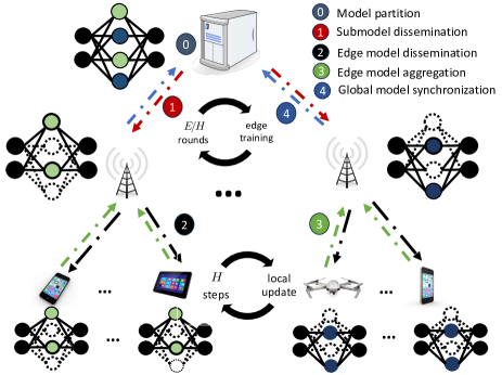
Inspired by IST [9], we develop a hierarchical federated submodel training algorithm termed HIST, by incorporating hierarchical FedAvg and submodel partitioning. The overview of HIST is presented in Fig. 1 and Algorithm 1. The global cloud server periodically aggregates the models from the edge servers, while each edge server periodically aggregates the models from the clients within the corresponding cell. The key difference with the conventional HFL is that, clients do not need to store, update, and exchange the full model in HIST.

Specifically, in the beginning of $t/E$-th global round where $t$ represents the iteration number of clients and $E$ denotes the period of the global aggregation, the cloud server initiates the training process by partitioning the current global model $\bar{\bm{x}}^{t}$ into $N$ disjoint submodels:

$$\bar{\bm{x}}^{t}_{j}=\bm{p}_{j}^{t}\odot\bar{\bm{x}}^{t},\forall j\in\{1,2,\ldots,N\},$$ (2)

where $\odot$ denotes a Hadamard Product operation, $\bar{\bm{x}}^{t}_{j}$ represents the $j$-th submodel for cell $j$, and $\bm{p}_{j}^{t}$ is a mask that has either $0$ or $1$ in its element and satisfying

$$\bm{p}_{j}^{t}\odot\bm{p}_{j^{\prime}}^{t}=\bm{0},\forall j^{\prime}\neq j,~{}\text{and}~{}\sum_{i=1}^{N}\bm{p}_{j}^{t}=\bm{1}.$$ (3)

These submodels are then distributed to the edge servers, and each edge server subsequently disseminates submodel $\bar{\bm{x}}^{t}_{j}$ to the clients within its coverage, such that ${\bm{x}}^{t}_{i}=\bar{\bm{x}}^{t}_{j},\forall i\in\mathcal{C}_{j}$. Once the clients receive the most recent model from the server, they start training with their local datasets. The essential steps performed by clients, edge servers, and the global server in our proposed algorithm are outlined as follows:

Clients: Clients first compute stochastic gradients with respect to their corresponding submodels, and then update the local models for $H$ steps via the following iteration:

$${\bm{x}}^{t+1}_{i}={\bm{x}}^{t}_{i}-\gamma{\bm{p}}^{t}_{j}\odot\nabla l({\bm{x}}^{t}_{i},\xi_{i}),\forall i\in\mathcal{C}_{j},\forall j.$$ (4)

Note that ${\bm{p}}^{t}_{j}$ keeps invariant during one global round, i.e., ${\bm{p}}^{mE+e}_{j}={\bm{p}}^{mE}_{j}$, $\forall e=\{1,2,\ldots,E-1\}$, where $m$ denotes the number of the global rounds. Subsequently, clients upload the updated submodels to the edge server for edge model aggregation.

Edge Servers: After every $H$ steps of local submodel updates, each edge server aggregates the local models within its coverage as

$$\bar{\bm{x}}^{t\!+\!1}_{j}\leftarrow\frac{1}{n_{j}}\sum_{i\in\mathcal{C}_{j}}{\bm{x}}^{t\!+\!1}_{i},\forall j.$$ (5)

Subsequently, edge servers determine whether to upload the aggregated model to the cloud server or disseminate it to the clients. The criterion is whether the current iteration number $t+1$ of clients is divisible by $E$. If not, edge servers just disseminate the edge models in (5) to the corresponding clients; otherwise, edge servers upload their edge models to the cloud server.

Cloud Server: If the client’s current iteration number $t+1$ is a multiple of $E$, the cloud server aggregates the edge models from edge servers according to

$$\bar{\bm{x}}^{t\!+\!1}=\sum_{j}^{N}{\bm{p}}^{t}_{j}\odot\bar{\bm{x}}^{t\!+\!1}_{j}.$$ (6)

Subsequently, the cloud server partitions the global model $\bar{\bm{x}}^{t\!+\!1}$ based on newly generated masks $\bm{p}^{t\!+\!1}_{j}$

$$\bm{x}_{j}^{t\!+\!1}=\bm{p}^{t\!+\!1}_{j}\odot\bar{\bm{x}}^{t\!+\!1},\forall j\in\{1,2,\ldots,N\}.$$ (7)

Finally, $\bm{x}_{j}^{t\!+\!1}$ will be sent to edge server $j$ for initiating the next round of training. Here, it is worth emphasizing that $\bar{\bm{x}}^{t}$ is defined on $t\in\{mE\mid m\in\mathbb{N}\}$ while $\bar{\bm{x}}_{j}^{t}$ is defined on $t\in\{mH\mid m\in\mathbb{N}\}$.

Input: Initial masks $\{\bm{p}^{0}_{1},\bm{p}^{0}_{2},\ldots,\bm{p}^{0}_{N}\}$, initial models $\bar{\bm{x}}^{0}$, and ${\bm{x}}_{i}^{0}=\bar{\bm{x}}_{j}^{0}=\bm{p}^{0}_{j}\odot\bar{\bm{x}}^{0},\forall i\in\mathcal{C}_{j},\forall j$, learning rate $\gamma$

for $t\in\{0,1,\dots,T-1\}$  do

       for each cell and edge server in parallel do

             for each client $i\in\mathcal{C}_{j}$ in parallel do

                   Update local submodel ${\bm{x}}_{i}^{t\!+\!1}$ by (4)

             end for

            if $H\mid t\!+\!1$ then

                   Update edge model $\bar{\bm{x}}_{j}^{t\!+\!1}$ via (5)

                   if $E\mid t\!+\!1$ then

                         Upload $\bar{\bm{x}}_{j}^{t\!+\!1}$ to the cloud server

                  else

                         Disseminate $\bar{\bm{x}}^{t\!+\!1}_{j}$ to clients

                   end if

                  

             end if

            

       end for

      if $E\mid t\!+\!1$ then

             Update the global model $\bar{\bm{x}}^{t\!\small+\!1}$ via (6)

             Generate masks $\{\bm{p}^{t\!+\!1}_{j}\}$ under rule (3)

             Partition the global model by (7) and send the obtained submodels $\bar{\bm{x}}^{t\!+\!1}_{j}$ to clients within cell $j$, $\bm{x}_{i}^{t\!+\!1}\!=\bar{\bm{x}}^{t\!+\!1}_{j}$, $\forall i\in\mathcal{C}_{j},\forall j$

       end if

      

end for

Algorithm 1 Hierarchical Independent Submodel Training Algorthm

With the proposed algorithm, clients and edge servers are not required to store or manipulate the full model parameters. This enables HIST to reduce the communication, computation, and storage burdens of clients and edge servers compared to the conventional HFL.

III-B Communication Complexity Analysis

Let $L_{0}$ denote the transmission load of a full model. Each client sends its local model parameter to the corresponding edge server every $H$ iterations, where $H$ denotes the number of local updates. Assume that the mask size, defined as the number of non-zero entries of $\bm{p}^{t}_{j}$, is uniform among $N$ cells. In every $H$ iterations, the total communication load of all the clients within cell $j$ becomes $\frac{n_{j}L_{0}}{N}$, which corresponds to the communication complexity of edge server $j$. The average per-iteration communication load of each client and edge server is $\frac{L_{0}}{NH}$ and $\frac{n_{j}L_{0}}{NH}$, respectively. Additionally, for the cloud server, the communication complexity at every $E$ iterations is $L_{0}$. Under the methodology of HIST, the communication complexity of the cloud server is invariant to the number of edge servers. In summary, HIST reduces the communication consumption of the global server, edge server, and client to $\frac{1}{N}$ of what would be required by the standard hierarchical FedAvg algorithm.

IV Convergence Analysis

In this section, we provide convergence analysis for the proposed HIST algorithm. Although the proposed HIST algorithm shares a similar training process with the hierarchical FedAvg, we stress that the convergence proof for the latter one cannot be directly extended to our case that adopts submodel partitioning, due to the effect of the masks. Specifically, when comparing $\bm{p}_{j}^{t}\odot\nabla F_{i}(\bm{p}_{j}^{t}\odot\bm{x})$ and $\nabla F_{i}(\bm{x})$, the mask $\bm{p}_{j}^{t}$ compresses not only the gradient but also the model, while many existing works only investigate compressing the gradient. Theoretical analysis on the methods of compressing the model [16] is quite limited. Even in the single-cell scenario, existing proofs of IST [13, 14] rely on some stronger assumptions. Finally, the hierarchical architecture with both multiple steps of client update and multiple steps of edge training we consider makes the analysis further complicated.

IV-A Assumptions

We focus on a general non-convex loss function and consider a non-i.i.d data setting. Our theoretical analysis relies on the following assumptions.

Assumption 1.

The global loss function $f(\bm{x})$ has a lower bound $f_{*}$, i.e., $f(\bm{x})\geq f_{*},\forall\bm{x}.$

Assumption 2.

$F_{i}$ is differentiable and $L$-smooth, i.e., there exists a positive constant $L$ such that for any $\bm{x}$ and $\bm{y}$

$$\|\nabla F_{i}(\bm{x})-\nabla F_{i}(\bm{y})\|^{2}\leq L\|\bm{y}-\bm{x}\|,\forall i,$$ (8)

$$F_{i}(\bm{y})\leq F_{i}(\bm{x})+\left\langle\nabla F_{i}(\bm{x}),\bm{y}-\bm{x}\right\rangle+\frac{L}{2}\|\bm{y}-\bm{x}\|^{2},\forall i.$$

With Assumption 2, one can also claim that functions $f_{j}$, $\forall j$ and $f$ are $L$-smooth [17].

Assumption 3.

The stochastic gradient $\nabla l(\bm{x},\xi_{i})$ is an unbiased estimate of the true gradient, i.e., $\mathbb{E}_{\xi_{i}\sim\mathcal{D}_{i}}[\nabla l(\bm{x},\xi_{i})]=\nabla F_{i}(\bm{x}),\forall\bm{x}$.

Assumption 4.

The variance of the stochastic gradient $\nabla l(\bm{x},\xi_{i})$ is bounded as

$$\mathbb{E}_{\bm{\xi}_{i}\sim\mathcal{D}_{i}}\|\nabla l(\bm{x},\xi_{i})-\nabla F_{i}(\bm{x})\|^{2}\leq\sigma^{2},\forall\bm{x}.$$ (9)

Assumption 5.

The gradient dissimilarity between the global loss and each edge loss $f_{j}$ can be bounded by a constant $\delta_{1}^{2}$, i.e.,

$$\frac{1}{N}\sum_{j=1}^{N}\|\nabla f_{j}({\bm{x}})-\nabla f(\bm{x})\|^{2}\leq\delta_{1}^{2},\forall\bm{x}.$$ (10)

Assumption 6.

The gradient dissimilarity between the edge loss $f_{j}$ and each client loss $F_{i}(\bm{x})$ can be bounded by a constant $\delta_{2}^{2}$, i.e.,

$$\frac{1}{n_{j}}\sum_{i\in\mathcal{C}_{j}}\|\nabla F_{i}({\bm{x}})-\nabla f_{j}(\bm{x})\|^{2}\leq\delta_{2}^{2},\forall\bm{x},\forall j.$$ (11)

Assumptions 1-4, have been widely adopted in the context of stochastic non-convex and smooth settings [17]. Assumptions 5 and 6 serve to characterize the degree of data heterogeneity between different cells and clients, which is a common characteristic within the HFL literature [8].

IV-B Theoretical Results

When implementing HIST in practice, $\bar{\bm{x}}^{t}$ will not be computed unless $t$ is a multiple of $E$ as the global synchronization occurs every $E$ iterations. We establish the convergence properties of the proposed algorithm by characterizing the evolution of $\|\nabla f\left(\hat{\bm{x}}^{t}\right)\!\|^{2}$, $\hat{\bm{x}}^{t}\coloneqq\sum_{j=1}^{N}{\bm{p}}^{t}_{j}\odot\frac{1}{n_{j}}\sum_{i\in\mathcal{C}_{j}}{\bm{x}}^{t}_{i},t=\{0,1,2,\ldots,T-1\}$, to see how fast the model converges to the stationary point of the general non-convex loss function. The sequence $\{\hat{\bm{x}}^{t}\!\mid\!t=0,1,2,\ldots,T-1\}$ we use for analysis serves as a virtual global model, which is commonly employed to monitor the convergence of distributed algorithms with delayed global synchronization [18]. Now we state the following main theorem.

Theorem 1.

Suppose that Assumptions 1-6 hold, the masks $\{\bm{p}_{1}^{t},\bm{p}_{2}^{t},\ldots,\bm{p}_{N}^{t}\}$ are uniformly and randomly generated based on (3), $N\geq 2$, and the step size satisfies

$$\gamma\leq \min\left\{\frac{1}{32E\sqrt{N-1}L},\frac{\tilde{N}}{NHL},\frac{1}{NH^{2}L},\frac{1}{(N+1)EL}\right\}.$$ (12)

Then, HIST achieves the following convergence behavior for non-convex loss functions:

$$\frac{1}{T}\sum_{t=0}^{T-1}\mathbb{E}\left\|\nabla f(\hat{\bm{x}}^{t})\right\|^{2}\leq 4\frac{f(\bar{\bm{x}}_{0})-f_{*}}{\gamma}+50\gamma\tilde{N}L\sigma^{2}$$

$$+\!24\gamma L\delta_{2}^{2}\!+\!12\delta_{1}^{2}\!+\!24(N\!-\!1)L^{2}\frac{E}{T}\sum_{m=0}^{T/E\!-\!1}\!\mathbb{E}\left\|\!\bar{\bm{x}}^{mE}\!\right\|^{2},$$ (13)

where $\tilde{N}=\sum_{j=1}^{N}\frac{1}{n_{j}}$, and $\bar{\bm{x}}_{mE}$ is the synchronized global model generated by our HIST algorithm.

Theorem 1 presents the optimality gap for the time-averaged squared gradient norm. The first term in this upper bound exhibits the influence of the initial optimality gap on convergence performance. The second term reveals the impact of the variance of stochastic gradients on convergence, which can be mitigated by increasing the batch size when computing stochastic gradients. The third and fourth terms indicate that the non-i.i.d. characteristics within the cell and across cells affect convergence performance. The last term demonstrates that the norms of synchronized global models also influence the optimality gap. Note that the last two terms are induced by submodel partition. In addition, the step size $\gamma$ is a configurable parameter that impacts the first three terms of the derived upper bound. Plugging an appropriate step size into Theorem 1 gives rise to the following corollary.

Corollary 1.

Suppose that Assumptions 1-6 hold, the masks $\{\bm{p}_{1}^{t},\bm{p}_{2}^{t},\ldots,\bm{p}_{N}^{t}\}$ are uniformly and randomly generated based on (3), $N\geq 2$, and let the step size $\gamma=(T\tilde{N})^{-\!\frac{1}{2}}$ in which $T$ is large enough to satisfy (12). Then, the HIST algorithm satisfies

$$\frac{1}{T}\sum_{t=0}^{T-1}\mathbb{E}\left\|\nabla f(\hat{\bm{x}}^{t})\right\|^{2}\leq\mathcal{O}\left(\tilde{N}^{\frac{1}{2}}T^{-\frac{1}{2}}\right)+\mathcal{O}\left(T^{-\frac{1}{2}}\right)$$

$$+12\delta_{1}^{2}+24(N-1)L^{2}\frac{E}{T}\sum_{m=0}^{T/E-1}\mathbb{E}\left\|\bar{\bm{x}}^{mE}\right\|^{2},$$ (14)

where $\tilde{N}$ and $\bar{\bm{x}}^{mE}$ are described in Theorem 1.

Remark 1.

In Corollary 1, the retention of $\tilde{N}$ within the convergence rate expression is motivated by the possibility of an arbitrary relationship between the number of clients in each cell, denoted as $n_{j}$, and the total number of cells, denoted as $N$. When the number of clients in each cell is of a comparable magnitude or greater than the total number of cells, the convergence rate of the diminishing terms in the derived upper bound is primarily determined by $\mathcal{O}\left(T^{-\frac{1}{2}}\right)$. However, if the number of clients in each cell is significantly smaller in relation to the total number of cells, $\tilde{N}$ becomes influential, and the convergence rate is dominated by $\mathcal{O}\left(\tilde{N}^{\frac{1}{2}}T^{-\frac{1}{2}}\right)$.

IV-C Discussions

Non-diminishing bound: With the step size chosen in Corollary 1, the first three terms in (1) will diminish to zero as long as the number of total iterations, i.e., $T$, is large enough. The rest two terms are non-diminishing parts that arise due to submodel training. One can claim that HIST can converge to the neighborhood of a stationary point of the non-convex loss function under the aforementioned conditions. A similar phenomenon has also been reported in the single-cell case [9, 13, 15]. The bound enables us to explore the performance-resource trade-off, where more detailed discussions will be provided in the next paragraph.

The choice of $N$: As $N$ increases, i.e., as the overall clients in the system are divided into more cells during training, the size of the submodels gets smaller, providing a more lightweight model to the edge servers and clients. As a result, the training costs including computation, communication, and storage will be reduced at each iteration. However, as observed in Corollary 1, a large $N$ causes the sequence to deviate further from the stationary point. Overall, there is a trade-off between the convergence performance and computation, communication, and storage costs.

The optimal values of $H$ and $E$: The choices of $H$ and $E$ impact the communication frequency. As $H$ increases, the aggregation frequency at the edge servers will become smaller, reducing the communication load between clients and the edge server. On the other hand, a large $E$ induces fewer global synchronizations, which releases the communication burden between edge servers and the cloud server. However, these values cannot be infinitely large. The maximum value of $H$ and $E$ can be derived from the condition of the step size $\gamma$. Specifically, to make the step size $\gamma=(T\tilde{N})^{-\!\frac{1}{2}}$ in Corollary 1 satisfy (12), $H$ and $E$ can be set as on the order of $\min\left\{\mathcal{O}\left((\tilde{N}T)^{\frac{1}{4}}N^{-\!\frac{1}{2}}\right),\mathcal{O}\left(\tilde{N}^{\frac{3}{2}}T^{\frac{1}{2}}N^{-1}\right)\right\}$ and $\mathcal{O}\left((\tilde{N}T)^{\frac{1}{2}}N^{-\!1}\right)$ at most, respectively.

V Simulations

In this section, we conduct experiments to evaluate the performance of the proposed HIST algorithm.

V-A Simulation Settings

We consider an image classification task on Fashion-MNIST using a two-layer fully connected neural network. In this model, we configure the input layer to have $784$ neurons, corresponding to the size of the input image, and the output layer to have $10$ neurons, which matches the number of classes. Additionally, we employ a hidden layer with $300$ neurons. The cloud server partitions these hidden neurons to construct different submodels. Let the submodels share the same size with each other, which can be achieved by uniformly and randomly partitioning the hidden neurons.

We consider a setup with $60$ clients evenly distributed across $N$ cells, where $N\in\{2,3,4,5\}$. We consider two practical data distribution settings: (i) the fully non-i.i.d. case and (ii) the case with i.i.d data across cells but non-i.i.d data across the clients within the same cell. For the former case, the client’s dataset construction follows the approach outlined in [2]. The process begins by sorting the training samples based on their corresponding labels. Following this, the training dataset is partitioned into $120$ shards, with each shard containing $500$ samples. Subsequently, each client is assigned $2$ shards, ensuring that each client’s dataset comprises $1000$ samples. For the latter, we first uniformly and randomly divide the entire training set into $N$ parts, corresponding to $N$ cells, and then distribute each part to the clients within the respective cell in a non-i.i.d. manner following the former case.

(a) Fully non-i.i.d.

(b) Cell i.i.d., client non-i.i.d.

Figure 2: The impact of the number of cells $N$ on the convergence performance.

(a) Fully non-i.i.d.

(b) Cell i.i.d., client non-i.i.d.

Figure 3: Communication cost for achieving a testing accuracy of $75\%$.

V-B Experiment Results and Discussions

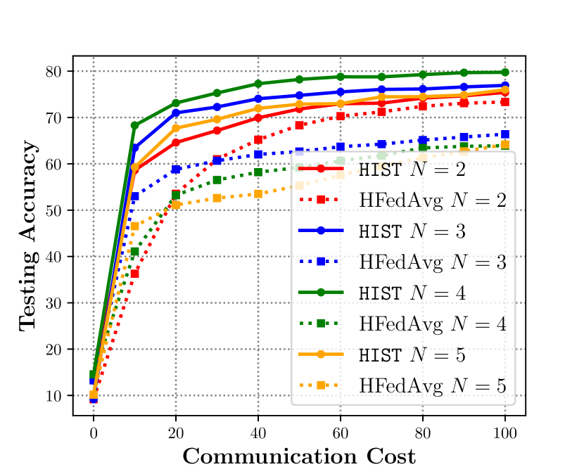
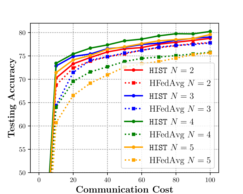
Comparison with Baselines: In Fig. 2, we compare our proposed HIST algorithm with the traditional hierarchical FedAvg (denoted as HFedAvg in our figures) where the full model is communicated over the network. We compare their performance in terms of testing accuracy under different numbers of cells, $N\in\{2,3,4,5\}$. The x-axis here represents the communication load which quantifies the volume of parameters transmitted by each client, where the unit is set to the load of a full-model transmission. For each client, the communication cost per global round is equal to $\frac{1}{N}\frac{E}{H}$ times the load of a full-model transmission. Here, $E/H$ represents the number of edge aggregations per global round. We set $H$ and $E$ to $40$ and $200$, respectively. As shown in Figs. 2(a) and 2(b), the proposed HIST algorithm outperforms hierarchical FedAvg in terms of testing accuracy at the same levels of communication consumption for both data distribution settings. Additionally, as $N$ increases, the non-i.i.d. extent of data among clients becomes more pronounced, leading to performance degradation for hierarchical FedAvg. In contrast, the proposed HIST achieves a higher testing accuracy when $N$ increases from $N=2$ to $N=4$. This is because, for HIST, the per-round communication cost per client decreases as the number of cells increases. However, when we increase the number of cells to $N=5$, HIST also suffers performance degradation. This can be attributed to the submodel getting too small for effectively handling the task, highlighting the trade-off between training costs and testing accuracy, which is also consistent with our theoretical results.

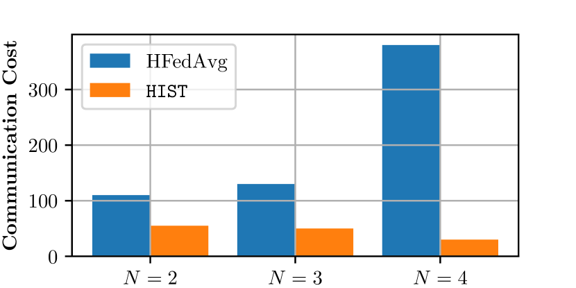
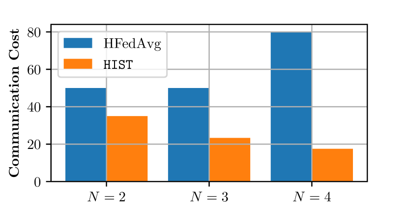
Fig. 3 compares the communication cost of HIST and hierarchical FedAvg for achieving the desired accuracy under both data distribution scenarios. This experiment was carried out with $H=40$ and $E=200$. The desired testing accuracy is set to be $75\%$. The Y-axis measures the size of parameters transmitted by each client during the training process as in the x-axis of Fig. 2. It is observed that HIST needs less communication to achieve the preset accuracy, which demonstrates the efficiency of the proposed algorithm over hierarchical FedAvg. In addition, as the number of cells increases from $N=2$ to $N=4$, the communication cost shows a decreasing trend, which forms a sharp comparison with hierarchical FedAvg. This further demonstrates the advantage of the proposed HIST algorithm.

(a) Fully non-i.i.d.

(b) Cell i.i.d., client non-i.i.d.

Figure 4: The impacts of aggregation periods $H$ and $E$ on the convergence performance.

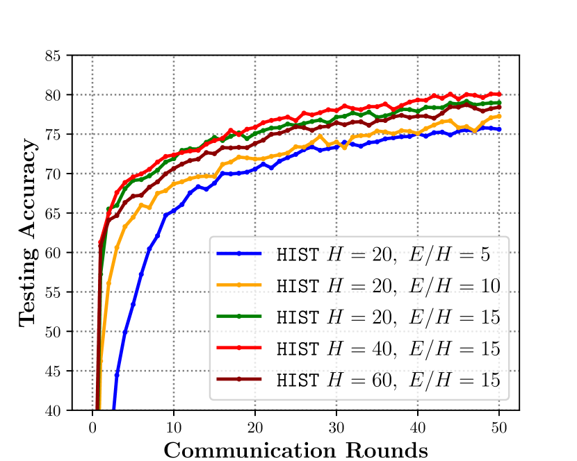
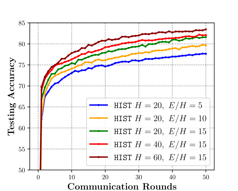
Effects of System Parameters: The impacts of the periods of the edge aggregation $H$ and the global synchronization $E/H$ on the convergence behavior are demonstrated in Fig. 4. The x-axis represents the number of global model synchronizations at the cloud server. We consider the $3$-cell case (i.e., $N=3$) where $60$ users are uniformly distributed across these cells without overlapping. As $E/H$ increases from $5$ to $10$ to $15$, HIST attain a better convergence performance, which is witnessed by both Figs. 4(a) and 4(b). This is because a large $E/H$ gives rise to a lower communication load for each round. When $H$ increases from $20$ to $40$, and from $40$ to $60$, Fig. 4(b) shows that the convergence speed of HIST first enjoys an acceleration and then a degradation, where the latter is induced by data heterogeneity. This phenomenon also fits well with our theory, where we show that there is an upper bound for the number of local updates. Fig. 4(b) shows that HIST has a better performance as $H$ increases from $40$ to $60$. This is because this data distribution exhibits lower data heterogeneity, which allows for a larger number of local updates.

VI Conclusion

In this paper, we developed a hierarchical federated submodel training algorithm termed HIST, that is efficient in terms of communication, computation, and storage by integrating independent model training with local training. We investigated its convergence behavior with uniform submodel partitioning under non-convex loss functions and non-i.i.d. data settings, and characterized the impacts of non-i.i.d. extent, the number of periods of edge and global aggregations, and the number of cells on the convergence performance. We show that HIST converges with rate $\max\left\{\mathcal{O}\left(\tilde{N}^{\frac{1}{2}}T^{-\!\frac{1}{2}}\right),\mathcal{O}\left(T^{-\!\frac{1}{2}}\right)\right\}$ to a neighborhood of a stationary point of the global loss function. Simulation results on two practical data distribution settings show that HIST is able to achieve the target accuracy much faster with less training costs, compared to the standard hierarchical FedAvg.

Appendices

VI-A Proof of Theorem 1

For analysis, we introduce virtual iterates $\hat{\bm{x}}^{t}_{j}\coloneqq\frac{1}{n_{j}}\sum_{i\in\mathcal{C}_{j}}{\bm{x}}^{t}_{i}$, $t=\{0,1,2,\ldots,T-1\}$, $\forall j$ which denotes the average of local models within cell $j$ and $\hat{\bm{x}}^{t}\coloneqq\sum_{j=1}^{N}{\bm{p}}^{t}_{j}\odot\hat{\bm{x}}^{t}_{j}$ which represents the vitually synchronized global model.

The proof of Theorem 1 relies on the following three lemmas which are proved in the next subsection.

Lemma 1.

Suppose that Assumptions 2-5 hold, the masks $\{\bm{p}_{1}^{t},\bm{p}_{2}^{t},\ldots,\bm{p}_{N}^{t}\}$ are uniformly and randomly generated based on (3), $N\geq 2$, and $\gamma\leq\frac{1}{L}$, then the virtual iterate $\hat{\bm{x}}^{t}$ satisfy

$$\mathbb{E}[f(\hat{\bm{x}}^{t+1})]\leq \mathbb{E}[f(\hat{\bm{x}}^{t})]-\frac{\gamma}{2}\mathbb{E}\left\|\nabla f(\hat{\bm{x}}^{t})\right\|^{2}+\frac{\gamma^{2}L\sigma^{2}}{2}\tilde{N}+\frac{3\gamma}{2}\delta_{1}^{2}$$ (15)

$$+\frac{3\gamma L^{2}}{2}\left\{\sum_{j=1}^{N}\mathbb{E}\left\|\hat{\bm{x}}^{t}-\hat{\bm{x}}^{t}_{j}\right\|^{2}+\sum_{j=1}^{N}\frac{1}{n_{j}}\sum_{i\in\mathcal{C}_{j}}\mathbb{E}\left\|\hat{\bm{x}}^{t}_{j}-{\bm{x}}^{t}_{i}\right\|^{2}\right\}.$$

Lemma 2.

Suppose that Assumptions 2-5 hold, the masks $\{\bm{p}_{1}^{t},\bm{p}_{2}^{t},\ldots,\bm{p}_{N}^{t}\}$ are uniformly and randomly generated based on (3), and $\gamma\leq\frac{1}{EL\sqrt{54(N+1)}}$, then the difference between the edge models and the global model can be bounded as

$$\frac{1}{T}\sum_{t=0}^{T-1}\sum_{j=1}^{N}\mathbb{E}\left\|\hat{\bm{x}}^{t}-\hat{\bm{x}}^{t}_{j}\right\|^{2}\leq \frac{1}{3}\frac{1}{T}\sum_{t=0}^{T-1}\sum_{j=1}^{N}\frac{1}{n_{j}}\sum_{i\in\mathcal{C}_{j}}\mathbb{E}\left\|\hat{\bm{x}}^{t}_{j}-{\bm{x}}^{t}_{i}\right\|^{2}+162\gamma^{2}E^{2}(N-1)\frac{1}{T}\sum_{t=0}^{T-1}\mathbb{E}\left\|\nabla f\left(\hat{\bm{x}}^{t}\right)\right\|^{2}$$ (16)

$$+108\gamma^{2}(N+1)E^{2}\delta_{1}^{2}+6\gamma^{2}(N+1)\tilde{N}E\sigma^{2}+4(N-1)\frac{E}{T}\sum_{m=0}^{T/E-1}\mathbb{E}\left\|\bar{\bm{x}}^{mE}\right\|^{2}.$$

Lemma 3.

Suppose that Assumptions 2-4 and 6 hold and $\gamma\leq\frac{1}{\sqrt{18}HL}$, then the difference between the local models and the edge models can be bounded as

$$\frac{1}{T}\sum_{t=1}^{T-1}\sum_{j=1}^{N}\frac{1}{n_{j}}\sum_{i\in\mathcal{C}_{j}}\mathbb{E}\left\|\hat{\bm{x}}^{t}_{j}-{\bm{x}}^{t}_{i}\right\|^{2}\leq\frac{3}{2}\gamma^{2}NH\sigma^{2}+3\gamma^{2}NH^{2}\delta_{2}^{2}.$$ (17)

Lemma 1 characterizes the dynamics of the global loss function. Lemmas 2 and 3 characterize the upper bound of the diversity between the virtual global model and edge models and between the virtual edge model and local models, respectively. With these lemmas, we can prove Theorem 1 as follows. First, reorganizing the inequality provided in Lemma 1, we have

$$\mathbb{E}\left\|\nabla f(\hat{\bm{x}}^{t})\right\|^{2}\leq 2\frac{\mathbb{E}[f(\hat{\bm{x}}^{t})]-\mathbb{E}[f(\hat{\bm{x}}^{t+1})]}{\gamma}+\gamma L\sigma^{2}\tilde{N}+3\delta_{1}^{2}$$ (18)

$$+3L^{2}\left\{\sum_{j=1}^{N}\mathbb{E}\left\|\hat{\bm{x}}^{t}-\hat{\bm{x}}^{t}_{j}\right\|^{2}+\sum_{j=1}^{N}\frac{1}{n_{j}}\sum_{i\in\mathcal{C}_{j}}\mathbb{E}\left\|\hat{\bm{x}}^{t}_{j}-{\bm{x}}^{t}_{i}\right\|^{2}\right\}.$$

Telescoping the above inequalities from $t=0$ to $T-1$, we have

$$\frac{1}{T}\sum_{t=0}^{T-1}\mathbb{E}\left\|\nabla f(\hat{\bm{x}}^{t})\right\|^{2}\leq 2\frac{f(\bar{\bm{x}}^{0})-\mathbb{E}[f(\hat{\bm{x}}^{T})]}{\gamma}+\gamma L\sigma^{2}\tilde{N}+3\delta_{1}^{2}+3L^{2}\left(D_{e}+D_{c}\right),$$ (19)

where $D_{e}=\frac{1}{T}\sum_{t=0}^{T-1}\sum_{j=1}^{N}\mathbb{E}\left\|\hat{\bm{x}}^{t}-\hat{\bm{x}}^{t}_{j}\right\|^{2}$ and $D_{c}=\frac{1}{T}\sum_{t=1}^{T-1}\sum_{j=1}^{N}\frac{1}{n_{j}}\sum_{i\in\mathcal{C}_{j}}\mathbb{E}\left\|\hat{\bm{x}}^{t}_{j}-{\bm{x}}^{t}_{i}\right\|^{2}$.

According to Lemma 2, we have

$$D_{e}+D_{c}\leq \frac{4}{3}D_{c}+162\gamma^{2}E^{2}(N-1)\frac{1}{T}\sum_{t=0}^{T-1}\mathbb{E}\left\|\nabla f\left(\hat{\bm{x}}^{t}\right)\right\|^{2}+108\gamma^{2}(N+1)E^{2}\delta_{1}^{2}$$ (20)

$$+6\gamma^{2}(N+1)\tilde{N}E\sigma^{2}+4(N-1)\frac{E}{T}\sum_{m=0}^{T/E-1}\mathbb{E}\left\|\bar{\bm{x}}^{mE}\right\|^{2}.$$

Combining the (19), (20), and Lemma 3, we have

$$\left(1-486\gamma^{2}E^{2}(N-1)L^{2}\right)\frac{1}{T}\sum_{t=0}^{T-1}\mathbb{E}\left\|\nabla f(\hat{\bm{x}}^{t})\right\|^{2}\leq 2\frac{f(\bar{\bm{x}}^{0})-\mathbb{E}[f(\hat{\bm{x}}^{T})]}{\gamma}+\gamma L\sigma^{2}\tilde{N}+3\delta_{1}^{2}$$ (21)

$$+6L^{2}(\gamma^{2}NH\sigma^{2}+2\gamma^{2}NH^{2}\delta_{2}^{2})+324\gamma^{2}(N+1)E^{2}L^{2}\delta_{1}^{2}+18\gamma^{2}(N+1)\tilde{N}EL^{2}\sigma^{2}$$

$$+12(N-1)L^{2}\frac{E}{T}\sum_{m=0}^{T/E-1}\mathbb{E}\left\|\bar{\bm{x}}^{mE}\right\|^{2}.$$

As $\gamma\leq\frac{1}{EL\sqrt{972(N-1)}}$, one can claim $1-972\gamma^{2}E^{2}(N-1)L^{2}\geq\frac{1}{2}$. Reorganizing (LABEL:combine_lemma13) gives rises to

$$\frac{1}{T}\sum_{t=0}^{T-1}\mathbb{E}\left\|\nabla f(\hat{\bm{x}}^{t})\right\|^{2}\leq 4\frac{f(\bar{\bm{x}}^{0})-\mathbb{E}[f(\hat{\bm{x}}^{T})]}{\gamma}+\left(2+12\gamma\frac{N}{\tilde{N}}HL+36\gamma(N+1)EL\right)\gamma L\sigma^{2}\tilde{N}+24\gamma^{2}NH^{2}L^{2}\delta_{2}^{2}$$ (22)

$$+\left(6+648\gamma^{2}(N+1)E^{2}L^{2}\right)\delta_{1}^{2}+24(N-1)L^{2}\frac{E}{T}\sum_{m=0}^{T/E-1}\mathbb{E}\left\|\bar{\bm{x}}^{mE}\right\|^{2}.$$

Recalling the setting of $\gamma$, we have

$$\frac{1}{T}\sum_{t=0}^{T-1}\mathbb{E}\left\|\nabla f(\hat{\bm{x}}^{t})\right\|^{2}\leq 4\frac{f(\bar{\bm{x}}^{0})-\mathbb{E}[f(\hat{\bm{x}}^{T})]}{\gamma}+50\gamma\tilde{N}L\sigma^{2}+24\gamma L\delta_{2}^{2}$$ (23)

$$+12\delta_{1}^{2}+24(N-1)L^{2}\frac{E}{T}\sum_{m=0}^{T/E-1}\mathbb{E}\left\|\bar{\bm{x}}^{mE}\right\|^{2},$$

where we use the inequality $32\sqrt{N-1}>\sqrt{108(N+1)}$, $\forall N\geq 2.$ Combining the above inequality with Assumption 1 gives rise to Theorem 1.

VI-B Proof of Lemmas

Before proving the above lemmas, we introduce some notations. Denote $\mathbb{E}_{t}$ as an expectation conditioned on the historical information up to the start of the $t$-th iteration. Denote $\mathbb{E}_{t}^{p}$ as an expectation over masks $\{\bm{p}_{j}^{t}\}_{j=1}^{N}$. Let $\bm{g}^{t}_{i}$ denote the stochastic gradient $\nabla l(\bm{x}_{i}^{t},\xi_{i})$, $\xi_{i}\in\mathcal{D}_{i}$. In addition, we present two facts that will be used in this subsection.

Fact 1.

Suppose that masks generated by rule (3) are uniform among $\{1,2,\dots,N\}$, i.e., $\|\bm{p}_{j}\|_{1}=\frac{d}{N},\forall j$, then

$$\mathbb{E}[\bm{p}_{j}\odot\bm{z}]=\frac{1}{N}\|\bm{z}\|^{2},~{}\forall j.$$

Proof.

$$\mathbb{E}[\|\bm{p}_{j}\odot\bm{z}\|^{2}]=\mathbb{E}[\sum_{k=1}^{d}([p_{j}]_{k}z_{k})^{2}]=\mathbb{E}[\sum_{k=1}^{d}([p_{j}]_{k}z_{k})^{2}]=\sum_{k=1}^{d}\mathbb{E}[([p_{j}]_{k}z_{k})^{2}]=\sum_{k=1}^{d}\frac{1}{N}z_{k}^{2}=\frac{1}{N}\|\bm{z}\|^{2},$$

where $[p_{j}]_{k}$ and $z_{k}$ represent the $k$-th elements of $\bm{p}_{j}$ and $\bm{z}$, respectively. ∎

Fact 2.

Any masks $\{\bm{p}_{j}\}_{j=1}^{N}$ generated by rule (3) satisfy

$$\sum_{j=1}^{N}\|\bm{p}_{j}\odot\bm{z}-\bm{z}\|^{2}=(N-1)\|\bm{z}\|^{2}.$$

Proof.

$$\sum_{j=1}^{N}\|\bm{p}_{j}\odot\bm{z}-\bm{z}\|^{2}=\sum_{j=1}^{N}\{\|\bm{p}_{j}\odot\bm{z}\|-2\langle\bm{p}_{j}\odot\bm{z},\bm{z}\rangle+\|\bm{z}\|^{2}\}=(N-1)\|\bm{z}\|^{2}.$$

∎

VI-B1 Proof of Lemma 1

Based on the virtual iteration $\hat{\bm{x}}^{t+1}=\hat{\bm{x}}^{t}-\sum_{j=1}^{N}{\bm{p}}^{t}_{j}\odot\frac{1}{n_{j}}\sum_{i\in\mathcal{C}_{j}}\gamma\bm{g}^{t}_{i}$ and Assumption 2, we have

$$\mathbb{E}_{t}[f(\hat{\bm{x}}^{t+1})]\leq f(\hat{\bm{x}}^{t})\underbrace{-\mathbb{E}_{t}\left\langle\nabla f(\hat{\bm{x}}^{t}),\sum_{j=1}^{N}{\bm{p}}^{t}_{j}\odot\frac{1}{n_{j}}\sum_{i\in\mathcal{C}_{j}}\gamma\bm{g}^{t}_{i}\right\rangle}_{T_{1}}+\frac{L}{2}\underbrace{\mathbb{E}_{t}\left\|\sum_{j=1}^{N}{\bm{p}}^{t}_{j}\odot\frac{1}{n_{j}}\sum_{i\in\mathcal{C}_{j}}\gamma\bm{g}^{t}_{i}\right\|^{2}}_{T_{2}}.$$ (24)

Utilizing Assumption 3, i.e., $\mathbb{E}[\bm{g}^{t}_{i}]=\nabla F_{i}({\bm{x}}^{t}_{i})$ and the fact that $\mathbb{E}\left\|\bm{z}\right\|^{2}=\mathbb{E}\left\|\bm{z}-\mathbb{E}[\bm{z}]\right\|^{2}+\mathbb{E}\left\|\mathbb{E}[\bm{z}]\right\|^{2}$, we rewrite $T_{2}$ as follows

$$T_{2}= \gamma^{2}\mathbb{E}_{t}\left\|\sum_{j=1}^{N}{\bm{p}}^{t}_{j}\odot\frac{1}{n_{j}}\sum_{i\in\mathcal{C}_{j}}\bm{g}^{t}_{i}-\sum_{j=1}^{N}{\bm{p}}^{t}_{j}\odot\frac{1}{n_{j}}\sum_{i\in\mathcal{C}_{j}}\nabla F_{i}({\bm{x}}^{t}_{i})\right\|^{2}+\gamma^{2}\mathbb{E}_{t}^{p}\left\|\sum_{j=1}^{N}{\bm{p}}^{t}_{j}\odot\frac{1}{n_{j}}\sum_{i\in\mathcal{C}_{j}}\nabla F_{i}({\bm{x}}^{t}_{i})\right\|^{2}.$$ (25)

As there is no overlapping between any two different masks in the same round, we have

$$T_{2}= \gamma^{2}\sum_{j=1}^{N}\mathbb{E}_{t}\left\|{\bm{p}}^{t}_{j}\odot\frac{1}{n_{j}}\sum_{i\in\mathcal{C}_{j}}\bm{g}^{t}_{i}-{\bm{p}}^{t}_{j}\odot\frac{1}{n_{j}}\sum_{i\in\mathcal{C}_{j}}\nabla F_{i}({\bm{x}}^{t}_{i})\right\|^{2}+\gamma^{2}\mathbb{E}_{t}^{p}\left\|\sum_{j=1}^{N}{\bm{p}}^{t}_{j}\odot\frac{1}{n_{j}}\sum_{i\in\mathcal{C}_{j}}\nabla F_{i}({\bm{x}}^{t}_{i})\right\|^{2}$$ (26)

$$= \gamma^{2}\sum_{j=1}^{N}\frac{1}{n_{j}^{2}}\sum_{i\in\mathcal{C}_{j}}\mathbb{E}_{t}\left\|{\bm{p}}^{t}_{j}\odot\left(\bm{g}^{t}_{i}-\nabla F_{i}({\bm{x}}^{t}_{i})\right)\right\|^{2}+\gamma^{2}\mathbb{E}_{t}^{p}\left\|\sum_{j=1}^{N}{\bm{p}}^{t}_{j}\odot\frac{1}{n_{j}}\sum_{i\in\mathcal{C}_{j}}\nabla F_{i}({\bm{x}}^{t}_{i})\right\|^{2}$$

$$\leq \gamma^{2}\sigma^{2}\left(\sum_{j=1}^{N}\frac{1}{n_{j}}\right)+\gamma^{2}\mathbb{E}_{t}^{p}\left\|\sum_{j=1}^{N}{\bm{p}}^{t}_{j}\odot\frac{1}{n_{j}}\sum_{i\in\mathcal{C}_{j}}\nabla F_{i}({\bm{x}}^{t}_{i})\right\|^{2},$$

where the second equality holds because $\mathbb{E}_{t}\langle\bm{g}^{t}_{i}-\nabla F_{i}({\bm{x}}^{t}_{i}),\bm{g}^{t}_{i^{\prime}}-\nabla F_{i^{\prime}}({\bm{x}}^{t}_{i^{\prime}})\rangle=0,\forall{i^{\prime}}\neq i$ and the inequality comes from Assumption 4. Utilizing $\mathbb{E}_{t}[\bm{g}^{t}_{i}]=\nabla F_{i}({\bm{x}}^{t}_{i})$ again, we rewrite $T_{1}$ as follows

$$T_{1}= -\gamma\mathbb{E}_{t}^{p}\left\langle\nabla f(\hat{\bm{x}}^{t}),\sum_{j=1}^{N}{\bm{p}}^{t}_{j}\odot\frac{1}{n_{j}}\sum_{i\in\mathcal{C}_{j}}\nabla F_{i}({\bm{x}}^{t}_{i})\right\rangle$$ (27)

$$= \frac{\gamma}{2}\left\{\mathbb{E}_{t}^{p}\left\|\nabla f(\hat{\bm{x}}^{t})-\sum_{j=1}^{N}{\bm{p}}^{t}_{j}\odot\frac{1}{n_{j}}\sum_{i\in\mathcal{C}_{j}}\nabla F_{i}({\bm{x}}^{t}_{i})\right\|^{2}-\left\|\nabla f(\hat{\bm{x}}^{t})\right\|^{2}-\mathbb{E}_{t}^{p}\left\|\sum_{j=1}^{N}{\bm{p}}^{t}_{j}\odot\frac{1}{n_{j}}\sum_{i\in\mathcal{C}_{j}}\nabla F_{i}({\bm{x}}^{t}_{i})\right\|^{2}\right\}.$$

Plugging $T_{1}$ and $T_{2}$ into (24) and utilizing $\gamma\leq\frac{1}{L}$ give the following inequality

$$\mathbb{E}_{t}[f(\hat{\bm{x}}^{t+1})]\leq f(\hat{\bm{x}}^{t})-\frac{\gamma}{2}\left\|\nabla f(\hat{\bm{x}}^{t})\right\|^{2}+\frac{\gamma^{2}L\sigma^{2}}{2}\left(\sum_{j=1}^{N}\frac{1}{n_{j}}\right)+\frac{\gamma}{2}\underbrace{\mathbb{E}_{t}^{p}\left\|\nabla f(\hat{\bm{x}}^{t})-\sum_{j=1}^{N}{\bm{p}}^{t}_{j}\odot\frac{1}{n_{j}}\sum_{i\in\mathcal{C}_{j}}\nabla F_{i}({\bm{x}}^{t}_{i})\right\|^{2}}_{T_{3}}.$$ (28)

Based on the facts that $\nabla f(\hat{\bm{x}}^{t})=\sum_{j}^{N}{\bm{p}}^{t}_{j}\odot\nabla f(\hat{\bm{x}}^{t})$ and $\|\sum_{j=1}^{N}{\bm{p}}^{t}_{j}\odot\bm{z}_{j}\|^{2}=\sum_{j=1}^{N}\|{\bm{p}}^{t}_{j}\odot\bm{z}_{j}\|^{2}$, we can rewrite $T_{3}$ as

$$T_{3}= \mathbb{E}_{t}^{p}\left\|\sum_{j=1}^{N}{\bm{p}}^{t}_{j}\odot\left(\nabla f(\hat{\bm{x}}^{t})-\frac{1}{n_{j}}\sum_{i\in\mathcal{C}_{j}}\nabla F_{i}({\bm{x}}^{t}_{i})\right)\right\|^{2}$$ (29)

$$= \sum_{j=1}^{N}\mathbb{E}_{t}^{p}\left\|{\bm{p}}^{t}_{j}\odot\left(\nabla f(\hat{\bm{x}}^{t})-\frac{1}{n_{j}}\sum_{i\in\mathcal{C}_{j}}\nabla F_{i}({\bm{x}}^{t}_{i})\right)\right\|^{2}.$$

By inserting a zero term $0=\mp\nabla f_{j}(\hat{\bm{x}}^{t})\mp\nabla f_{j}(\hat{\bm{x}}^{t}_{j})$ into the right of the above expression, we have

$$T_{3}= \sum_{j=1}^{N}\mathbb{E}_{t}^{p}\left\|{\bm{p}}^{t}_{j}\odot\left(\nabla f(\hat{\bm{x}}^{t})\mp\nabla f_{j}(\hat{\bm{x}}^{t})\mp\nabla f_{j}(\hat{\bm{x}}^{t}_{j})-\frac{1}{n_{j}}\sum_{i\in\mathcal{C}_{j}}\nabla F_{i}({\bm{x}}^{t}_{i})\right)\right\|^{2}$$ (30)

$$\leq 3\sum_{j=1}^{N}\mathbb{E}_{t}^{p}\left\|{\bm{p}}^{t}_{j}\odot\left(\nabla f(\hat{\bm{x}}^{t})-\nabla f_{j}(\hat{\bm{x}}^{t})\right)\right\|^{2}+3\sum_{j=1}^{N}\mathbb{E}_{t}^{p}\left\|{\bm{p}}^{t}_{j}\odot\left(\nabla f_{j}(\hat{\bm{x}}^{t})-\nabla f_{j}(\hat{\bm{x}}^{t}_{j})\right)\right\|^{2}$$

$$+3\sum_{j=1}^{N}\mathbb{E}_{t}^{p}\left\|{\bm{p}}^{t}_{j}\odot\left(\nabla f_{j}(\hat{\bm{x}}^{t}_{j})-\frac{1}{n_{j}}\sum_{i\in\mathcal{C}_{j}}\nabla F_{i}({\bm{x}}^{t}_{i})\right)\right\|^{2}$$

$$= 3\frac{1}{N}\sum_{j=1}^{N}\left\|\nabla f(\hat{\bm{x}}^{t})-\nabla f_{j}(\hat{\bm{x}}^{t})\right\|^{2}+3\sum_{j=1}^{N}\mathbb{E}_{t}^{p}\left\|{\bm{p}}^{t}_{j}\odot\left(\nabla f_{j}(\hat{\bm{x}}^{t})-\nabla f_{j}(\hat{\bm{x}}^{t}_{j})\right)\right\|^{2}$$

$$+3\sum_{j=1}^{N}\mathbb{E}_{t}^{p}\left\|{\bm{p}}^{t}_{j}\odot\left(\frac{1}{n_{j}}\sum_{i\in\mathcal{C}_{j}}\nabla F_{i}(\hat{\bm{x}}^{t}_{j})-\frac{1}{n_{j}}\sum_{i\in\mathcal{C}_{j}}\nabla F_{i}({\bm{x}}^{t}_{i})\right)\right\|^{2}$$

$$\leq 3\delta_{1}^{2}+3\sum_{j=1}^{N}\mathbb{E}_{t}^{p}\left\|\nabla f_{j}(\hat{\bm{x}}^{t})-\nabla f_{j}(\hat{\bm{x}}^{t}_{j})\right\|^{2}+3\sum_{j=1}^{N}\mathbb{E}_{t}^{p}\left\|\frac{1}{n_{j}}\sum_{i\in\mathcal{C}_{j}}\nabla F_{i}(\hat{\bm{x}}^{t}_{j})-\frac{1}{n_{j}}\sum_{i\in\mathcal{C}_{j}}\nabla F_{i}({\bm{x}}^{t}_{i})\right\|^{2}$$

$$\leq 3\delta_{1}^{2}+3\sum_{j=1}^{N}\mathbb{E}_{t}^{p}\left\|\nabla f_{j}(\hat{\bm{x}}^{t})-\nabla f_{j}(\hat{\bm{x}}^{t}_{j})\right\|^{2}+3\sum_{j=1}^{N}\frac{1}{n_{j}}\sum_{i\in\mathcal{C}_{j}}\mathbb{E}_{t}^{p}\left\|\nabla F_{i}(\hat{\bm{x}}^{t}_{j})-\nabla F_{i}({\bm{x}}^{t}_{i})\right\|^{2}$$

$$\leq 3\delta_{1}^{2}+3L^{2}\sum_{j=1}^{N}\mathbb{E}_{t}^{p}\left\|\hat{\bm{x}}^{t}-\hat{\bm{x}}^{t}_{j}\right\|^{2}+3L^{2}\sum_{j=1}^{N}\frac{1}{n_{j}}\sum_{i\in\mathcal{C}_{j}}\mathbb{E}_{t}^{p}\left\|\hat{\bm{x}}^{t}_{j}-{\bm{x}}^{t}_{i}\right\|^{2},$$

where the first inequality comes from Cauchy-Swarchz inequality, the second equality holds due to Fact 1, the second inequality follows Assumption 5 and the fact that $\|p\odot\bm{z}\|^{2}\leq\|\bm{z}\|^{2}$, the third inequality follows Jensen’s inequality, and the final one follows Assumption 2.

Plugging the above upper bound of $T_{3}$ into (28) and taking an expectation over all the randomness, we will obtain Lemma 1.

VI-B2 Proof of Lemma 2

Without the loss generality, we consider $t\in[mE,(m+1)E)$. For notation ease, we denote $T_{4}=\sum_{j=1}^{N}\mathbb{E}\left\|\hat{\bm{x}}^{t}-\hat{\bm{x}}^{t}_{j}\right\|^{2}$. Based on the fact that the global model synchronization every $E$ local iterations, $T_{4}$ can be rewritten as

$$T_{4}= \sum_{j=1}^{N}\mathbb{E}\left\|\bar{\bm{x}}^{mE}-\gamma\sum_{\tau=mE}^{t-1}\sum_{j=1}^{N}\frac{1}{n_{j}}\sum_{i\in\mathcal{C}_{j}}{\bm{p}}^{\tau}_{j}\odot g_{i}^{\tau}-\left(\bar{\bm{x}}^{mE}_{j}-\gamma\sum_{\tau=mE}^{t-1}\frac{1}{n_{j}}\sum_{i\in\mathcal{C}_{j}}{\bm{p}}^{\tau}_{j}\odot g_{i}^{\tau}\right)\right\|^{2}.$$

Recalling Cauchy-Swartz inequality and Fact 2, we have

$$T_{4}\leq 2\sum_{j=1}^{N}\left\|\bar{\bm{x}}^{mE}-\bar{\bm{x}}^{mE}_{j}\right\|^{2}+2\gamma^{2}\sum_{j=1}^{N}\mathbb{E}\left\|\sum_{\tau=mE}^{t-1}\sum_{j=1}^{N}\frac{1}{n_{j}}\sum_{i\in\mathcal{C}_{j}}{\bm{p}}^{\tau}_{j}\odot g_{i}^{\tau}-\sum_{\tau=mE}^{t-1}\frac{1}{n_{j}}\sum_{i\in\mathcal{C}_{j}}{\bm{p}}^{\tau}_{j}\odot g_{i}^{\tau}\right\|^{2}$$ (31)

$$= 2(N-1)\left\|\bar{\bm{x}}^{mE}\right\|^{2}+2\gamma^{2}\underbrace{\sum_{j=1}^{N}\mathbb{E}\left\|\sum_{\tau=mE}^{t-1}\sum_{j=1}^{N}\frac{1}{n_{j}}\sum_{i\in\mathcal{C}_{j}}{\bm{p}}^{\tau}_{j}\odot g_{i}^{\tau}-\sum_{\tau=mE}^{t-1}\frac{1}{n_{j}}\sum_{i\in\mathcal{C}_{j}}{\bm{p}}^{\tau}_{j}\odot g_{i}^{\tau}\right\|^{2}}_{T_{5}}.$$

For $T_{5}$, we have

$$T_{5}= \sum_{j=1}^{N}\mathbb{E}\left\|\sum_{\tau=mE}^{t-1}\sum_{j=1}^{N}\frac{1}{n_{j}}\sum_{i\in\mathcal{C}_{j}}{\bm{p}}^{\tau}_{j}\odot\left(g_{i}^{\tau}\mp\nabla F_{i}({\bm{x}}_{i}^{\tau})\right)-\sum_{\tau=mE}^{t-1}\frac{1}{n_{j}}\sum_{i\in\mathcal{C}_{j}}{\bm{p}}^{\tau}_{j}\odot\left(g_{i}^{\tau}\mp\nabla F_{i}({\bm{x}}_{i}^{\tau})\right)\right\|^{2}$$ (32)

$$\leq 3\sum_{j=1}^{N}\mathbb{E}\left\|\sum_{\tau=mE}^{t-1}\sum_{j=1}^{N}\frac{1}{n_{j}}\sum_{i\in\mathcal{C}_{j}}{\bm{p}}^{\tau}_{j}\odot\left(g_{i}^{\tau}-\nabla F_{i}({\bm{x}}_{i}^{\tau})\right)\right\|^{2}+3\sum_{j=1}^{N}\mathbb{E}\left\|\sum_{\tau=mE}^{t-1}\frac{1}{n_{j}}\sum_{i\in\mathcal{C}_{j}}{\bm{p}}^{\tau}_{j}\odot\left(g_{i}^{\tau}-\nabla F_{i}({\bm{x}}_{i}^{\tau})\right)\right\|^{2}$$

$$+3\sum_{j=1}^{N}\mathbb{E}\left\|\sum_{\tau=mE}^{t-1}\sum_{j=1}^{N}\frac{1}{n_{j}}\sum_{i\in\mathcal{C}_{j}}{\bm{p}}^{\tau}_{j}\odot\nabla F_{i}({\bm{x}}_{i}^{\tau})-\sum_{\tau=mE}^{t-1}\frac{1}{n_{j}}\sum_{i\in\mathcal{C}_{j}}{\bm{p}}^{\tau}_{j}\odot\nabla F_{i}({\bm{x}}_{i}^{\tau})\right\|^{2}$$

$$= 3N\sum_{\tau=mE}^{t-1}\sum_{j=1}^{N}\frac{1}{n_{j}^{2}}\sum_{i\in\mathcal{C}_{j}}\mathbb{E}\left\|{\bm{p}}^{\tau}_{j}\odot\left(g_{i}^{\tau}-\nabla F_{i}({\bm{x}}_{i}^{\tau})\right)\right\|^{2}+3\sum_{j=1}^{N}\sum_{\tau=mE}^{t-1}\frac{1}{n_{j}^{2}}\sum_{i\in\mathcal{C}_{j}}\mathbb{E}\left\|{\bm{p}}^{\tau}_{j}\odot\left(g_{i}^{\tau}-\nabla F_{i}({\bm{x}}_{i}^{\tau})\right)\right\|^{2}$$

$$+3\sum_{j=1}^{N}\mathbb{E}\left\|\sum_{\tau=mE}^{t-1}\sum_{j=1}^{N}\frac{1}{n_{j}}\sum_{i\in\mathcal{C}_{j}}{\bm{p}}^{\tau}_{j}\odot\nabla F_{i}({\bm{x}}_{i}^{\tau})-\sum_{\tau=mE}^{t-1}\frac{1}{n_{j}}\sum_{i\in\mathcal{C}_{j}}{\bm{p}}^{\tau}_{j}\odot\nabla F_{i}({\bm{x}}_{i}^{\tau})\right\|^{2}$$

$$\leq 3(t-mE)\sum_{\tau=mE}^{t-1}\sum_{j=1}^{N}\underbrace{\mathbb{E}\left\|\sum_{j=1}^{N}\frac{1}{n_{j}}\sum_{i\in\mathcal{C}_{j}}{\bm{p}}^{\tau}_{j}\odot\nabla F_{i}({\bm{x}}_{i}^{\tau})-\frac{1}{n_{j}}\sum_{i\in\mathcal{C}_{j}}{\bm{p}}^{\tau}_{j}\odot\nabla F_{i}({\bm{x}}_{i}^{\tau})\right\|^{2}}_{T_{6}}$$

$$+3(N+1)(t-mE)\sigma^{2}\sum_{j=1}^{N}\frac{1}{n_{j}},$$

where the first inequality comes from Cauchy-Swartz inequality, the second equality follows [19, Lemma 2], and the second inequality follows Cauchy-Swartz inequality and Assumption 4.

For $T_{6}$, we have

$$T_{6}= \mathbb{E}\left\|\sum_{j=1}^{N}\frac{1}{n_{j}}\sum_{i\in\mathcal{C}_{j}}\bm{p}_{j}^{\tau}\odot\left(\nabla F_{i}\left(\bm{x}_{i}^{\tau}\right)\mp\nabla F_{i}\left(\hat{\bm{x}}^{\tau}_{j}\right)\right)-\frac{1}{n_{j}}\sum_{i\in\mathcal{C}_{j}}\bm{p}_{j}^{\tau}\odot\left(\nabla F_{i}\left(\bm{x}_{i}^{\tau}\right)\mp\nabla F_{i}\left(\hat{\bm{x}}^{\tau}_{j}\right)\right)\right\|^{2}$$ (33)

$$\leq 3\mathbb{E}\left\|\sum_{j=1}^{N}\frac{1}{n_{j}}\sum_{i\in\mathcal{C}_{j}}\bm{p}_{j}^{\tau}\odot\left(\nabla F_{i}\left(\bm{x}_{i}^{\tau}\right)-\nabla F_{i}\left(\hat{\bm{x}}^{\tau}_{j}\right)\right)\right\|^{2}+3\mathbb{E}\left\|\sum_{j=1}^{N}\frac{1}{n_{j}}\sum_{i\in\mathcal{C}_{j}}\bm{p}_{j}^{\tau}\odot\nabla F_{i}\left(\hat{\bm{x}}^{\tau}_{j}\right)-\frac{1}{n_{j}}\sum_{i\in\mathcal{C}_{j}}\bm{p}_{j}^{\tau}\odot\nabla F_{i}\left(\hat{\bm{x}}^{\tau}_{j}\right)\right\|^{2}$$

$$+3\mathbb{E}\left\|\frac{1}{n_{j}}\sum_{i\in\mathcal{C}_{j}}\bm{p}_{j}^{\tau}\odot\left(\nabla F_{i}\left(\bm{x}_{i}^{\tau}\right)-\nabla F_{i}\left(\hat{\bm{x}}^{\tau}_{j}\right)\right)\right\|^{2}$$

$$\leq 3NL^{2}\sum_{j=1}^{N}\frac{1}{n_{j}}\sum_{i\in\mathcal{C}_{j}}\mathbb{E}\left\|\bm{x}_{i}^{\tau}-\hat{\bm{x}}^{\tau}_{j}\right\|^{2}+3\underbrace{\mathbb{E}\left\|\sum_{j=1}^{N}\frac{1}{n_{j}}\sum_{i\in\mathcal{C}_{j}}\bm{p}_{j}^{\tau}\odot\nabla F_{i}\left(\hat{\bm{x}}^{\tau}_{j}\right)-\frac{1}{n_{j}}\sum_{i\in\mathcal{C}_{j}}\bm{p}_{j}^{\tau}\odot\nabla F_{i}\left(\hat{\bm{x}}^{\tau}_{j}\right)\right\|^{2}}_{T_{7}}$$

$$+3L^{2}\frac{1}{n_{j}}\sum_{i\in\mathcal{C}_{j}}\mathbb{E}\left\|\bm{x}_{i}^{\tau}-\hat{\bm{x}}^{\tau}_{j}\right\|^{2},$$

where the first inequality comes from Cauchy-Swartz inequality and Jensen’s inequality and the second inequality comes from Jensen’s inequality and $L$-smoothness of $F_{i}$. For $T_{7}$, we have

$$T_{7}= \mathbb{E}\left\|\sum_{j=1}^{N}\frac{1}{n_{j}}\sum_{i\in\mathcal{C}_{j}}\bm{p}_{j}^{\tau}\odot\left(\nabla F_{i}\left(\hat{\bm{x}}^{\tau}_{j}\right)\mp\nabla F_{i}\left(\hat{\bm{x}}^{\tau}\right)\right)-\frac{1}{n_{j}}\sum_{i\in\mathcal{C}_{j}}\bm{p}_{j}^{\tau}\odot\left(\nabla F_{i}\left(\hat{\bm{x}}^{\tau}_{j}\right)\mp\nabla F_{i}\left(\hat{\bm{x}}^{\tau}\right)\right)\right\|^{2}$$ (34)

$$\leq 3\mathbb{E}\left\|\sum_{j=1}^{N}\bm{p}_{j}^{\tau}\odot\frac{1}{n_{j}}\sum_{i\in\mathcal{C}_{j}}\left(\nabla F_{i}\left(\hat{\bm{x}}^{\tau}_{j}\right)-\nabla F_{i}\left(\hat{\bm{x}}^{\tau}\right)\right)\right\|^{2}+3\mathbb{E}\left\|\frac{1}{n_{j}}\sum_{i\in\mathcal{C}_{j}}\bm{p}_{j}^{\tau}\odot\left(\nabla F_{i}\left(\hat{\bm{x}}^{\tau}_{j}\right)-\nabla F_{i}\left(\hat{\bm{x}}^{\tau}\right)\right)\right\|^{2}$$

$$+3\mathbb{E}\left\|\sum_{j=1}^{N}\frac{1}{n_{j}}\sum_{i\in\mathcal{C}_{j}}\bm{p}_{j}^{\tau}\odot\nabla F_{i}\left(\hat{\bm{x}}^{\tau}\right)-\frac{1}{n_{j}}\sum_{i\in\mathcal{C}_{j}}\bm{p}_{j}^{\tau}\odot\nabla F_{i}\left(\hat{\bm{x}}^{\tau}\right)\right\|^{2}$$

$$\leq 3\sum_{j=1}^{N}\frac{1}{n_{j}}\sum_{i\in\mathcal{C}_{j}}\mathbb{E}\left\|\nabla F_{i}\left(\hat{\bm{x}}^{\tau}_{j}\right)-\nabla F_{i}\left(\hat{\bm{x}}^{\tau}\right)\right\|^{2}+3\frac{1}{n_{j}}\sum_{i\in\mathcal{C}_{j}}\mathbb{E}\left\|\nabla F_{i}\left(\hat{\bm{x}}^{\tau}_{j}\right)-\nabla F_{i}\left(\hat{\bm{x}}^{\tau}\right)\right\|^{2}$$

$$+3\mathbb{E}\left\|\sum_{j=1}^{N}\bm{p}_{j}^{\tau}\odot\nabla f_{j}\left(\hat{\bm{x}}^{\tau}\right)-\bm{p}_{j}^{\tau}\odot\nabla f_{j}\left(\hat{\bm{x}}^{\tau}\right)\right\|^{2}$$

$$\leq 3L^{2}\sum_{j=1}^{N}\mathbb{E}\left\|\hat{\bm{x}}^{\tau}_{j}-\hat{\bm{x}}^{\tau}\right\|^{2}+3L^{2}\mathbb{E}\left\|\hat{\bm{x}}^{\tau}_{j}-\hat{\bm{x}}^{\tau}\right\|^{2}+3\underbrace{\mathbb{E}\left\|\sum_{j=1}^{N}\bm{p}_{j}^{\tau}\odot\nabla f_{j}\left(\hat{\bm{x}}^{\tau}\right)-\bm{p}_{j}^{\tau}\odot\nabla f_{j}\left(\hat{\bm{x}}^{\tau}\right)\right\|^{2}}_{T_{8}},$$

where the first inequality follows Cauchy-Swartz inequality, the second inequality comes from the fact that $\|\sum_{j}^{N}\bm{p}_{j}\odot\bm{z}_{j}\|^{2}=\sum_{j}^{N}\|\bm{p}_{j}\odot\bm{z}_{j}\|^{2}\leq\sum_{j}^{N}\|\bm{z}_{j}\|^{2}$ and Jensen’s inequality, and the final one holds due to Assumption 2.

Similarly, we bound $T_{8}$ as follows

$$T_{8}= \mathbb{E}\left\|\sum_{j=1}^{N}\bm{p}_{j}^{\tau}\odot\left(f_{j}\left(\hat{\bm{x}}^{\tau}\right)\mp f\left(\hat{\bm{x}}^{\tau}\right)\right)-\bm{p}_{j}^{\tau}\odot\left(\nabla f_{j}\left(\hat{\bm{x}}^{\tau}\right)\mp\nabla f\left(\hat{\bm{x}}^{\tau}\right)\right)\right\|^{2}$$ (35)

$$\leq 3\mathbb{E}\left\|\sum_{j=1}^{N}\bm{p}_{j}^{\tau}\odot\left(\nabla f_{j}\left(\hat{\bm{x}}^{\tau}\right)-\nabla f\left(\hat{\bm{x}}^{\tau}\right)\right)\right\|^{2}+3\mathbb{E}\left\|\bm{p}_{j}^{\tau}\odot\left(\nabla f_{j}\left(\hat{\bm{x}}^{\tau}\right)-\nabla f\left(\hat{\bm{x}}^{\tau}\right)\right)\right\|^{2}$$

$$+3\mathbb{E}\left\|\bm{p}_{j}^{\tau}\odot\nabla f\left(\hat{\bm{x}}^{\tau}\right)-\sum_{j=1}^{N}\bm{p}_{j}^{\tau}\odot\nabla f\left(\hat{\bm{x}}^{\tau}\right)\right\|^{2}$$

$$= 3\sum_{j=1}^{N}\mathbb{E}\left\|\bm{p}_{j}^{\tau}\odot\left(\nabla f_{j}\left(\hat{\bm{x}}^{\tau}\right)-\nabla f\left(\hat{\bm{x}}^{\tau}\right)\right)\right\|^{2}+3\mathbb{E}\left\|\bm{p}_{j}^{\tau}\odot\left(\nabla f_{j}\left(\hat{\bm{x}}^{\tau}\right)-\nabla f\left(\hat{\bm{x}}^{\tau}\right)\right)\right\|^{2}+3\mathbb{E}\left\|\bm{p}_{j}^{\tau}\odot\nabla f\left(\hat{\bm{x}}^{\tau}\right)-\nabla f\left(\hat{\bm{x}}^{\tau}\right)\right\|^{2}$$

$$\leq \frac{3}{N}\sum_{j=1}^{N}\mathbb{E}\left\|\nabla f_{j}\left(\hat{\bm{x}}^{\tau}\right)-\nabla f\left(\hat{\bm{x}}^{\tau}\right)\right\|^{2}+\frac{3}{N}\mathbb{E}\left\|\nabla f_{j}\left(\hat{\bm{x}}^{\tau}\right)-\nabla f\left(\hat{\bm{x}}^{\tau}\right)\right\|^{2}+3\mathbb{E}\left\|\bm{p}_{j}^{\tau}\odot\nabla f\left(\hat{\bm{x}}^{\tau}\right)-\nabla f\left(\hat{\bm{x}}^{\tau}\right)\right\|^{2},$$

where the last inequality follows Fact 1.

Combining the upper bounds of (32), (33), (34), and (35), we have

$$T_{5}\leq 9(N+1)L^{2}(t-mE)\sum_{\tau=mE}^{t-1}T_{9}+27(N+1)L^{2}(t-mE)\sum_{\tau=mE}^{t-1}T_{4}$$ (36)

$$+81(N\!+\!1)(t\!-\!mE)^{2}\frac{1}{N}\sum_{j=1}^{N}\mathbb{E}\left\|\nabla f_{j}\left(\hat{\bm{x}}^{\tau}\right)\!-\!\nabla f\left(\hat{\bm{x}}^{\tau}\right)\right\|^{2}\!+\!81(t\!-\!mE)\sum_{\tau=mE}^{t-1}\sum_{j=1}^{N}\mathbb{E}\left\|\bm{p}_{j}^{\tau}\odot\nabla f\left(\hat{\bm{x}}^{\tau}\right)\!-\!\nabla f\left(\hat{\bm{x}}^{\tau}\right)\right\|^{2}$$

$$+3(N+1)(t-mE)\sigma^{2}\sum_{j=1}^{N}\frac{1}{n_{j}},$$

where $T_{9}=\sum_{j=1}^{N}\frac{1}{n_{j}}\sum_{i\in\mathcal{C}_{j}}\mathbb{E}\left\|\hat{\bm{x}}^{t}_{j}-{\bm{x}}^{t}_{i}\right\|^{2}$. Next, utilizing Assumption 5, Fact 2, and (31), we have

$$T_{4}\leq 18\gamma^{2}(N+1)L^{2}(t-mE)\sum_{\tau=mE}^{t-1}T_{9}+54\gamma^{2}(N+1)L^{2}(t-mE)\sum_{\tau=mE}^{t-1}T_{4}$$ (37)

$$+162\gamma^{2}(N\!+\!1)(t\!-\!mE)^{2}\delta_{1}^{2}\!+\!162\gamma^{2}(N\!-\!1)(t\!-\!mE)\sum_{\tau=mE}^{t-1}\mathbb{E}\left\|\nabla f\left(\hat{\bm{x}}^{\tau}\right)\right\|^{2}$$

$$+6\gamma^{2}(N+1)(t-mE)\sigma^{2}\sum_{j=1}^{N}\frac{1}{n_{j}}+2(N-1)\left\|\bar{\bm{x}}^{mE}\right\|^{2}.$$

Taking a time average of the above inequality gives rise to

$$\frac{1}{T}\sum_{t=0}^{T-1}T_{4}\leq 9\gamma^{2}(N+1)E^{2}L^{2}\frac{1}{T}\sum_{t=0}^{T-1}T_{9}+27\gamma^{2}(N+1)E^{2}L^{2}\frac{1}{T}\sum_{t=0}^{T-1}T_{4}$$ (38)

$$+81\gamma^{2}(N-1)E^{2}\frac{1}{T}\sum_{t=0}^{T-1}\mathbb{E}\left\|\nabla f\left(\hat{\bm{x}}^{t}\right)\right\|^{2}+54\gamma^{2}(N+1)E^{2}\delta_{1}^{2}$$

$$+3\gamma^{2}(N+1)\tilde{N}E\sigma^{2}+2(N-1)\frac{E}{T}\sum_{m=0}^{T/E-1}\mathbb{E}\left\|\bar{\bm{x}}^{mE}\right\|^{2},$$

where we use the fact that $1^{2}+2^{2}+\ldots+(E-1)^{2}\leq\frac{E^{3}}{3}$ and $1+2+\ldots+(E-1)=\frac{E^{2}}{2}$. Reorganizing the above inequality, we obtain

$$\left(1-27\gamma^{2}(N+1)E^{2}L^{2}\right)\frac{1}{T}\sum_{t=0}^{T-1}T_{4}\leq 9\gamma^{2}(N+1)E^{2}L^{2}\frac{1}{T}\sum_{t=0}^{T-1}T_{9}+81\gamma^{2}(N-1)E^{2}\frac{1}{T}\sum_{t=0}^{T-1}\mathbb{E}\left\|\nabla f\left(\hat{\bm{x}}^{t}\right)\right\|^{2}$$ (39)

$$+54\gamma^{2}(N+1)E^{2}\delta_{1}^{2}+3\gamma^{2}(N+1)\tilde{N}E\sigma^{2}+2(N-1)\frac{E}{T}\sum_{m=0}^{T/E-1}\mathbb{E}\left\|\bar{\bm{x}}^{mE}\right\|^{2},$$

As $\gamma\leq\frac{1}{EL\sqrt{54(N+1)}}$, we thus obtain Lemma 2.

VI-B3 Proof of Lemma 3

Without loss of generality, we consider $t\in[\alpha H,(\alpha+1)H)$. For notation ease, we denote $T_{9}=\sum_{j=1}^{N}\frac{1}{n_{j}}\sum_{i\in\mathcal{C}_{j}}\mathbb{E}\left\|\hat{\bm{x}}^{t}_{j}-{\bm{x}}^{t}_{i}\right\|^{2}$. As edge servers aggregate local models every $H$ local iterations, we can rewrite $T_{9}$ as

$$T_{9}= \gamma^{2}\sum_{j=1}^{N}\frac{1}{n_{j}}\sum_{i\in\mathcal{C}_{j}}\mathbb{E}\left\|\sum_{\tau=\alpha H}^{t-1}{\bm{p}}^{\tau}_{j}\odot\bm{g}_{i}^{\tau}-\sum_{\tau=\alpha H}^{t-1}{\bm{p}}^{\tau}_{j}\odot\frac{1}{n_{j}}\sum_{i\in\mathcal{C}_{j}}\bm{g}_{i}^{\tau}\right\|^{2}$$ (40)

$$= \gamma^{2}\sum_{j=1}^{N}\mathbb{E}\left[\underbrace{\frac{1}{n_{j}}\sum_{i\in\mathcal{C}_{j}}\left\|\sum_{\tau=\alpha H}^{t-1}{\bm{p}}^{\tau}_{j}\odot\bm{g}_{i}^{\tau}-\sum_{\tau=\alpha H}^{t-1}{\bm{p}}^{\tau}_{j}\odot\frac{1}{n_{j}}\sum_{i\in\mathcal{C}_{j}}\bm{g}_{i}^{\tau}\right\|^{2}}_{T_{10}}\right].$$

For $T_{10}$, we have

$$T_{10}\leq \frac{1}{n_{j}}\sum_{i\in\mathcal{C}_{j}}\left\|\sum_{\tau=\alpha H}^{t-1}\bm{g}_{i}^{\tau}\mp\sum_{\tau=\alpha H}^{t-1}\nabla F_{i}({\bm{x}}^{t}_{i})\mp\sum_{\tau=\alpha H}^{t-1}\frac{1}{n_{j}}\sum_{i\in\mathcal{C}_{j}}\nabla F_{i}({\bm{x}}^{t}_{i})-\sum_{\tau=\alpha H}^{t-1}\frac{1}{n_{j}}\sum_{i\in\mathcal{C}_{j}}\bm{g}_{i}^{\tau}\right\|^{2}$$ (41)

$$\leq 2\frac{1}{n_{j}}\sum_{i\in\mathcal{C}_{j}}\left\|\sum_{\tau=\alpha H}^{t-1}\bm{g}_{i}^{\tau}-\sum_{\tau=\alpha H}^{t-1}\nabla F_{i}({\bm{x}}^{t}_{i})-\sum_{\tau=\alpha H}^{t-1}\frac{1}{n_{j}}\sum_{i\in\mathcal{C}_{j}}\bm{g}_{i}^{\tau}+\sum_{\tau=\alpha H}^{t-1}\frac{1}{n_{j}}\sum_{i\in\mathcal{C}_{j}}\nabla F_{i}({\bm{x}}^{t}_{i})\right\|^{2}$$

$$+2\frac{1}{n_{j}}\sum_{i\in\mathcal{C}_{j}}\left\|\sum_{\tau=\alpha H}^{t-1}\nabla F_{i}({\bm{x}}^{t}_{i})-\sum_{\tau=\alpha H}^{t-1}\frac{1}{n_{j}}\sum_{i\in\mathcal{C}_{j}}\nabla F_{i}({\bm{x}}^{t}_{i})\right\|^{2}$$

$$\leq 2\frac{1}{n_{j}}\sum_{i\in\mathcal{C}_{j}}\left\|\sum_{\tau=\alpha H}^{t-1}\bm{g}_{i}^{\tau}-\sum_{\tau=\alpha H}^{t-1}\nabla F_{i}({\bm{x}}^{t}_{i})\right\|^{2}+2\frac{1}{n_{j}}\sum_{i\in\mathcal{C}_{j}}\left\|\sum_{\tau=\alpha H}^{t-1}\nabla F_{i}({\bm{x}}^{t}_{i})-\sum_{\tau=\alpha H}^{t-1}\frac{1}{n_{j}}\sum_{i\in\mathcal{C}_{j}}\nabla F_{i}({\bm{x}}^{t}_{i})\right\|^{2}$$

$$= 2\frac{1}{n_{j}}\sum_{i\in\mathcal{C}_{j}}\sum_{\tau=\alpha H}^{t-1}\left\|\bm{g}_{i}^{\tau}-\nabla F_{i}({\bm{x}}^{t}_{i})\right\|^{2}+2\frac{1}{n_{j}}\sum_{i\in\mathcal{C}_{j}}\left\|\sum_{\tau=\alpha H}^{t-1}\nabla F_{i}({\bm{x}}^{t}_{i})-\sum_{\tau=\alpha H}^{t-1}\frac{1}{n_{j}}\sum_{i\in\mathcal{C}_{j}}\nabla F_{i}({\bm{x}}^{t}_{i})\right\|^{2}$$

$$\leq 2(t-\alpha H)\sigma^{2}+2\underbrace{\frac{1}{n_{j}}\sum_{i\in\mathcal{C}_{j}}\left\|\sum_{\tau=\alpha H}^{t-1}\nabla F_{i}({\bm{x}}^{t}_{i})-\sum_{\tau=\alpha H}^{t-1}\frac{1}{n_{j}}\sum_{i\in\mathcal{C}_{j}}\nabla F_{i}({\bm{x}}^{t}_{i})\right\|^{2}}_{T_{11}},$$

where the third inequality follows that the fact that $\frac{1}{M}\sum\|\bm{z}_{m}-\frac{1}{M}\sum_{m=1}^{M}\bm{z}_{m}\|^{2}\leq\frac{1}{M}\sum\|\bm{z}_{m}\|^{2}$, the second equality follows [19, Lemma 2], and the final inequality comes from Assumption 4.

Next, we bound $T_{11}$.

$$T_{11}= \frac{1}{n_{j}}\sum_{i\in\mathcal{C}_{j}}\left\|\sum_{\tau=\alpha H}^{t-1}\nabla F_{i}({\bm{x}}^{t}_{i})\mp\sum_{\tau=\alpha H}^{t-1}\nabla F_{i}(\hat{\bm{x}}^{t}_{j})\mp\sum_{\tau=\alpha H}^{t-1}\frac{1}{n_{j}}\sum_{i\in\mathcal{C}_{j}}\nabla F_{i}(\hat{\bm{x}}^{t}_{j})-\sum_{\tau=\alpha H}^{t-1}\frac{1}{n_{j}}\sum_{i\in\mathcal{C}_{j}}\nabla F_{i}({\bm{x}}^{t}_{i})\right\|^{2}$$ (42)

$$\leq \frac{3}{n_{j}}\sum_{i\in\mathcal{C}_{j}}\left\|\sum_{\tau=\alpha H}^{t-1}\nabla F_{i}({\bm{x}}^{t}_{i})-\sum_{\tau=\alpha H}^{t-1}\nabla F_{i}(\hat{\bm{x}}^{t}_{j})\right\|^{2}+\frac{3}{n_{j}}\sum_{i\in\mathcal{C}_{j}}\left\|\sum_{\tau=\alpha H}^{t-1}\nabla F_{i}(\hat{\bm{x}}^{t}_{j})-\sum_{\tau=\alpha H}^{t-1}\frac{1}{n_{j}}\sum_{i\in\mathcal{C}_{j}}\nabla F_{i}(\hat{\bm{x}}^{t}_{j})\right\|^{2}$$

$$+\frac{3}{n_{j}}\sum_{i\in\mathcal{C}_{j}}\left\|\sum_{\tau=\alpha H}^{t-1}\frac{1}{n_{j}}\sum_{i\in\mathcal{C}_{j}}\nabla F_{i}(\hat{\bm{x}}^{t}_{j})-\sum_{\tau=\alpha H}^{t-1}\frac{1}{n_{j}}\sum_{i\in\mathcal{C}_{j}}\nabla F_{i}({\bm{x}}^{t}_{i})\right\|^{2}$$

$$\leq \frac{6}{n_{j}}(t-\alpha H)\sum_{i\in\mathcal{C}_{j}}\sum_{\tau=\alpha H}^{t-1}\left\|\nabla F_{i}({\bm{x}}^{t}_{i})-\nabla F_{i}(\hat{\bm{x}}^{t}_{j})\right\|^{2}+\frac{3}{n_{j}}(t-\alpha H)\sum_{i\in\mathcal{C}_{j}}\sum_{\tau=\alpha H}^{t-1}\left\|\nabla F_{i}(\hat{\bm{x}}^{t}_{j})-\frac{1}{n_{j}}\sum_{i\in\mathcal{C}_{j}}\nabla F_{i}(\hat{\bm{x}}^{t}_{j})\right\|^{2}$$

$$\leq \frac{6L^{2}}{n_{j}}(t-\alpha H)\sum_{i\in\mathcal{C}_{j}}\sum_{\tau=\alpha H}^{t-1}\left\|{\bm{x}}^{t}_{i}-\hat{\bm{x}}^{t}_{j}\right\|^{2}+3(t-\alpha H)^{2}\delta_{2}^{2},$$

where the first and second inequalities follow the Cauchy-Swartz inequality and the final one follows Assumptions 2 and 6.

Therefore, we have

$$T_{9}\leq 2\gamma^{2}N(t-\alpha H)\sigma^{2}+6\gamma^{2}N(t-\alpha H)^{2}\delta_{2}^{2}+12\gamma^{2}(t-\alpha H)L^{2}\sum_{\tau=\alpha H}^{t-1}T_{9}.$$ (43)

Taking the time average, we obtain

$$\frac{1}{T}\sum_{t=1}^{T-1}T_{9}\leq \gamma^{2}NH\sigma^{2}+2\gamma^{2}NH^{2}\delta_{2}^{2}+6\gamma^{2}HL^{2}\left(\frac{1}{T}\sum_{t=1}^{T-1}T_{9}\right).$$ (44)

As $\gamma\leq\frac{1}{HL\sqrt{18}}$, we thus have Lemma 3.

References

- [1] K. B. Letaief, Y. Shi, J. Lu, and J. Lu, “Edge artificial intelligence for 6g: Vision, enabling technologies, and applications,” IEEE Journal on Selected Areas in Communications, vol. 40, no. 1, pp. 5–36, 2021.
- [2] W. Fang, Z. Yu, Y. Jiang, Y. Shi, C. N. Jones, and Y. Zhou, “Communication-efficient stochastic zeroth-order optimization for federated learning,” IEEE Transactions on Wireless Communications, vol. 70, pp. 5058–5073, 2022.
- [3] L. Yuan, L. Sun, P. S. Yu, and Z. Wang, “Decentralized federated learning: A survey and perspective,” arXiv preprint arXiv:2306.01603, 2023.
- [4] B. McMahan, E. Moore, D. Ramage, S. Hampson, and B. A. y Arcas, “Communication-efficient learning of deep networks from decentralized data,” in Artificial intelligence and statistics, pp. 1273–1282, PMLR, 2017.
- [5] S. Wang, T. Tuor, T. Salonidis, K. K. Leung, C. Makaya, T. He, and K. Chan, “Adaptive federated learning in resource constrained edge computing systems,” IEEE journal on selected areas in communications, vol. 37, no. 6, pp. 1205–1221, 2019.
- [6] L. Liu, J. Zhang, S. Song, and K. B. Letaief, “Hierarchical federated learning with quantization: Convergence analysis and system design,” IEEE Transactions on Wireless Communications, vol. 22, no. 1, pp. 2–18, 2022.
- [7] W. Wen, Z. Chen, H. H. Yang, W. Xia, and T. Q. Quek, “Joint scheduling and resource allocation for hierarchical federated edge learning,” IEEE Transactions on Wireless Communications, vol. 21, no. 8, pp. 5857–5872, 2022.
- [8] J. Wang, S. Wang, R.-R. Chen, and M. Ji, “Demystifying why local aggregation helps: Convergence analysis of hierarchical sgd,” in Proceedings of the AAAI Conference on Artificial Intelligence, vol. 36, pp. 8548–8556, 2022.
- [9] B. Yuan, C. R. Wolfe, C. Dun, Y. Tang, A. Kyrillidis, and C. Jermaine, “Distributed learning of fully connected neural networks using independent subnet training,” Proceedings of the VLDB Endowment, vol. 15, no. 8, pp. 1581–1590, 2022.
- [10] C. R. Wolfe, J. Yang, F. Liao, A. Chowdhury, C. Dun, A. Bayer, S. Segarra, and A. Kyrillidis, “Gist: Distributed training for large-scale graph convolutional networks,” Journal of Applied and Computational Topology, pp. 1–53, 2023.
- [11] C. Dun, C. R. Wolfe, C. M. Jermaine, and A. Kyrillidis, “Resist: Layer-wise decomposition of resnets for distributed training,” in Uncertainty in Artificial Intelligence, pp. 610–620, PMLR, 2022.
- [12] E. Diao, J. Ding, and V. Tarokh, “Heterofl: Computation and communication efficient federated learning for heterogeneous clients,” in International Conference on Learning Representations, 2021.
- [13] A. Mohtashami, M. Jaggi, and S. Stich, “Masked training of neural networks with partial gradients,” in International Conference on Artificial Intelligence and Statistics, pp. 5876–5890, PMLR, 2022.
- [14] H. Zhou, T. Lan, G. Venkataramani, and W. Ding, “On the convergence of heterogeneous federated learning with arbitrary adaptive online model pruning,” arXiv preprint arXiv:2201.11803, 2022.
- [15] E. Shulgin and P. Richtárik, “Towards a better theoretical understanding of independent subnetwork training,” arXiv preprint arXiv:2306.16484, 2023.
- [16] A. Khaled and P. Richtárik, “Gradient descent with compressed iterates,” arXiv preprint arXiv:1909.04716, 2019.
- [17] A. Beck, First-order methods in optimization. SIAM, 2017.
- [18] S. U. Stich, “Local sgd converges fast and communicates little,” in International Conference on Learning Representations, 2019.
- [19] J. Wang, Q. Liu, H. Liang, G. Joshi, and H. V. Poor, “A novel framework for the analysis and design of heterogeneous federated learning,” IEEE Transactions on Signal Processing, vol. 69, pp. 5234–5249, 2021.