Machine Learning Infused Distributed Optimization for Coordinating Virtual Power Plant Assets

Abstract

Amid the increasing interest in the deployment of Distributed Energy Resources (DERs), the Virtual Power Plant (VPP) has emerged as a pivotal tool for aggregating diverse DERs and facilitating their participation in wholesale energy markets. These VPP deployments have been fueled by the Federal Energy Regulatory Commission’s Order 2222, which makes DERs and VPPs competitive across market segments. However, the diversity and decentralized nature of DERs present significant challenges to the scalable coordination of VPP assets. To address efficiency and speed bottlenecks, this paper presents a novel machine learning-assisted distributed optimization to coordinate VPP assets. Our method, named as $\mathcal{LOOP-MAC}$ (Learning to Optimize the Optimization Process for Multi-agent Coordination), adopts a multi-agent coordination perspective where each VPP agent manages multiple DERs and utilizes neural network approximators to expedite the solution search. The $\mathcal{LOOP-MAC}$ method employs a gauge map to guarantee strict compliance with local constraints, effectively reducing the need for additional post-processing steps. Our results highlight the advantages of $\mathcal{LOOP-MAC}$, showcasing accelerated solution times per iteration and significantly reduced convergence times. The $\mathcal{LOOP-MAC}$ method outperforms conventional centralized and distributed optimization methods in optimization tasks that require repetitive and sequential execution.

I Introduction

I-A Motivation

As global energy sectors transition towards sustainability, the role of Distributed Energy Resources (DERs) has become increasingly significant. However, the participation of DERs in competitive electricity markets remains a challenge [1]. While many DERs are capable of providing wholesale market services, they often individually fall short of the minimum size thresholds established by Independent System Operators (ISOs) and may not meet performance requirements [2]. As a solution to these challenges, Virtual Power Plants (VPPs) have emerged to aggregate diverse DERs, creating a unified operating profile for participation in wholesale markets and providing services to system operators [3]. Further promoting the aggregation of DERs, the Federal Energy Regulatory Commission’s (FERC’s) Order 2222, issued in September 2020, allowed DERs to compete on equal terms with other resources in ISO energy, capacity, and ancillary service markets [2]. The FERC regulatory advancement strengthens the position of DERs and VPPs in the market.

Despite their promising potential, the massive, decentralized, diverse, heterogeneous, and small-scale nature of DERs poses significant challenges to traditional centralized approaches, especially in terms of computational efficiency and speed. Centralized controls for VPPs require global information from all DERs, making them susceptible to catastrophic failures if centralized nodes fail and potentially compromising the privacy of DER owners’ information. To address these issues, there is a growing demand for efficient, scalable, distributed and decentralized optimization techniques. Our study aims to tackle these challenges and develop a solution that can efficiently harness the benefits of DERs, thereby unlocking the full potential of VPPs.

I-B Related Work

I-B1 VPP Functionalities and Objectives

VPPs act as aggregators for a variety of DERs, playing a pivotal role in mitigating integration barriers between DERs and grid operations [4]. In what folows, we will highlight recent insights gained from extensive research conducted on strategies for coordinating DERs within VPPs. For instance, optimization schemes for coordinating DERs within VPPs can be customized to achieve various objectives including:

• VPP’s self financial and operational objectives:

  • Maximizing revenue from energy trading across different markets [5, 6].

  • Decreasing operational and maintenance costs of operating VPPs [5, 6, 7, 8, 9, 10].

  • Optimizing load curtailment [11] or energy exportation [12].

  • Reducing end-user discomfort from joining demand response efforts [13].

  • Narrowing the discrepancy between actual power consumption and predetermined set points and schedules [14, 15].

  • Mitigating financial burden of operational risks [16, 17, 18, 19, 20].

• Contributing to system-level initiatives:

  • Curtailing greenhouse gas emissions [21, 22].

  • Advancing the reliability and resilience of the overall energy system [19, 20, 23].

I-B2 Shortcomings of Centralized Coordination Methods

Today’s centralized optimization methods are not designed to cope with decentralized, diverse, heterogeneous, and small-scale nature of DERs. Recent studies have shown that integrating DERs at scale may adversely impact today’s tools operation’s efficiency and performance speed [24].

Major challenges of centralized management strategies include:

• Scalability issues become more pronounced with the addition of more DERs to the network, resulting in increased computational demands due to the management of a growing set of variables

• Security and privacy risks as centralized decision-making models requires comprehensive data from all DERs [25].

• Severe system disruptions resulting from dependence on a single centralized node, as a failure in that node may pose a significant operational risk.

• Significant delays in the decision-making process due to the strain on the communication infrastructure, a situation worsened by continuous data communication and the intermittent nature of DERs.

• Adaptability challenges as the centralized systems struggle to provide timely responses to network changes. This limitation stems from their requirement for a comprehensive understanding of the entire system to make informed decisions [26].

• Logistical and political challenges given the diverse and intricate nature of DERs within a comprehensive centralized optimization strategy that spans across various regions and utilities [27].

In response to these challenges, there is a growing demand and interest in the development and implementation of efficient, scalable, and decentralized optimization approaches.

I-B3 State-of-the-art in Distributed Coordination

Distributed coordination methods organize DERs into clusters, with each one treated as an independent agent with capabilities for communication, computation, data storage, and operation, as demonstrated in previous work [28]. A distributed configuration enables DERs to function efficiently without dependence on a central controller. Distributed coordination paradigms, which leverage the autonomy of individual agents, have played a crucial role in the decentralized dispatch of DERs, as highlighted in recent surveys [25].

Among the numerous distributed optimization methods proposed in power systems, the Alternating Direction Method of Multipliers (ADMM) has gained popularity for its versatility across different optimization scenarios. Recent examples include a distributed model to minimize the dispatch cost of DERs in VPPs, while accounting for network constraints [20]. Another noteworthy contribution is a fully distributed methodology that, combines ADMM and consensus optimization protocols to address transmission line limits in VPPs [24]. Li et al. [29] introduced a decentralized algorithm to enable demand response optimization for electric vehicles within a VPP. Contributing to the robustness of VPPs, another decentralized algorithm based on message queuing has been proposed to enhance system resilience, particularly in cases of coordinator disruptions [30].

I-B4 Challenges of Existing Distributed Coordination Methods

Despite their many advantages, most distributed optimization techniques, even those with convergence guarantees, require significant parameter tuning to ensure numerical stability and practical convergence. Real-time energy markets impose operational constraints that require frequent updates, sometimes as frequently as every five minutes throughout the day, as indicated by [31]. The frequent update demands that the optimization of DERs dispatch within VPPs is resolved frequently and in a timely manner. Nevertheless, the iterative nature of these optimization techniques can significantly increase computation time, restricting their utility in time-sensitive scenarios. Moreover, the optimization performance may not necessarily improve, even when encountering identical or analogous dispatching problems frequently, leading to computational inefficiency.

To address these limitations, machine learning (ML) has been deployed to enhance the efficiency of optimization procedures, as discussed in [32]. The utilization of neural networks can expedite the search process and reduce the number of iterations needed to identify optimal solutions. Furthermore, neural approximators can continually enhance their performance as they encounter increasingly complex optimization challenges, as demonstrated in [33].

ML-assisted distributed optimizers can be broadly categorized into three distinct models: supervised learning, unsupervised learning, and reinforcement learning. In the realm of supervised learning, a data-driven method to expedite the convergence of ADMM in solving distributed DC optimal power flow is presented in [34], where authors employ penalty-based techniques to achieve local feasibility. Additional applications of supervised learning are demonstrated in [35] and [36], where ML algorithms are used to provide warm-start points for ADMM. On the other hand, unsupervised learning is exemplified in [37], where a learning-assisted asynchronous ADMM method is proposed, leveraging k-means for anomaly detection. Reinforcement learning has been applied to train neural network controllers for achieving DER voltage control [38], frequency control [39], and optimal transactions [40].

Although these studies showcase the potential of ML for adaptive, real-time DER optimization in decentralized VPP models, they do not fully develop ML-infused distributed optimization methods to improve computation speed while ensuring solution feasibility.

I-C Contributions

In this paper, we propose a ML-based to replace building blocks of the ADMM-based distributed optimization technique with neural approximators, a method termed $\mathcal{LOOP-MAC}$  (Learning to Optimize the Optimization Process for Multi-agent Coordination). We will employ our $\mathcal{LOOP-MAC}$  method to find a multi-agent solution for the power dispatch problem in DER coordination within a VPP. In the muti-agent VPP configuration, each agent may control multiple DERs. The proposed $\mathcal{LOOP-MAC}$  method enables each agent to predict local power profiles by communicating with its neighbors. All agents collaborate to achieve a near-optimal solution for power dispatch while adhering to both local and system-level constraints.

The utilization of neural networks expedites the search process and reduces the number of iterations required to identify optimal solutions. Additionally, unlike restoration-based methods, the $\mathcal{LOOP-MAC}$  approach doesn’t necessitate post-processing steps to enhance feasibility because local constraints are inherently enforced through a gauge mapping method [41], and coupled constraints are penalized through ADMM iterations.

II Problem formulation

II-A Compact Formulation

II-A1 The compact formulation for original optimization problem

The centralized optimization function is:

$$\min_{\mathbf{u}}f(\mathbf{u},\mathbf{x})~{}~{}\text{s.t.}~{}~{}\mathbf{u}\in\mathcal{S}(\mathbf{x})$$ (1)

where $\mathbf{u}=\bigoplus_{i}\mathbf{u}^{i}$ represents the collection of optimization variables across all agents. Note, $\bigoplus$ denotes vector concatenation, and $\mathbf{u}^{i}$ indicates the optimization variable vector of agent $i$. Similarly, $\mathbf{x}=\bigoplus_{i}\mathbf{x}^{i}$ encompasses all input parameters across agents, with $\mathbf{x}^{i}$ indicating the input parameter vector for agent $i$. The overall objective function is captured by $f=\sum_{i}f^{i}(\mathbf{x}^{i},\mathbf{u}^{i})$ where $f^{i}$ stands for the objective function of agent $i$. Lastly, $\mathcal{S}$ refers to the collection of all agent’s constraint sets.

II-A2 The compact formulation at the multi-agent-level

Here, we will introduce the agent-based method to distribute computation responsibilities among all agents. Let the variable vector of each agent, $\mathbf{u}^{i}$, consist of both local and global variables, which can be partitioned as $\mathbf{u}^{i}=[\mathbf{u}^{i}_{\texttt{l}},\mathbf{u}^{i}_{\texttt{g}}]$. Here, $\mathbf{u}^{i}_{\texttt{l}}$ captures the local variables of agent $i$, while $\mathbf{u}^{i}_{\texttt{g}}$ encapsulates the global variables shared among neighboring agents. To enable distributed computations, each agent $i$ maintains a local copy vector of other agents’ variables, $\mathbf{u}^{i}_{\texttt{g,Copy}}$, from which this vector mimics the global variables owned by neighboring agents.

Agent-level computations

Solving (1) in a distributed fashion requires agent $i$ to solve the following problem before communication.

$$\min_{\mathbf{u}^{i},\mathbf{u}^{i}_{\texttt{g,Copy}}}f^{i}([\mathbf{u}^{i}_{\texttt{l}},\mathbf{u}^{i}_{\texttt{g}}],\mathbf{u}^{i}_{\texttt{g,Copy}},\mathbf{x}^{i})$$ (2a)

s.t. $$\textup{local constraints: }\begin{bmatrix}\mathbf{u}^{i}\\ \mathbf{u}^{i}_{\texttt{g,Copy}}\end{bmatrix}\in\mathcal{S}_{\texttt{Local}}^{i}(\mathbf{x}^{i})$$ (2b)

$$\textup{consensus constraints: }\mathbf{u}^{i}_{\texttt{g,Copy}}=\mathbf{I}_{\texttt{c}}^{i}[\bigoplus_{j\neq i}\mathbf{u}^{j}_{\texttt{g}}]$$ (2c)

where $\mathcal{S}_{\texttt{Local}}^{i}$ denotes the agent $i$’s local constraint set. Here, $\mathbf{I}_{\texttt{c}}^{i}[\bigoplus_{j\neq i}\mathbf{u}^{j}_{\texttt{g}}]$ denotes the global variables owned by neighboring agents, and $\mathbf{I}_{\texttt{c}}^{i}$ is an element selector matrix. The distributed optimization process and intra-agent information exchange will ensure agreement among local copies of shared global variables.

Intra-agent Information Exchange

$$\textup{dual update:}\boldsymbol{\lambda}^{i^{[k]}}\!\!\!\!\!=\boldsymbol{\lambda}^{i^{[k-1]}}\!\!\!\!+\rho(\mathbf{u}^{i^{[k-1]}}_{\texttt{g,Copy}}-\mathbf{I}_{\texttt{c}}^{i}[\bigoplus_{j\neq i}\mathbf{u}_{\texttt{g}}^{j^{[k-1]}}])$$ (3)

$$\textup{primal optimization: }\begin{bmatrix}\mathbf{u}^{i^{[k]}}\\ \mathbf{u}^{i^{[k]}}_{\texttt{g,Copy}}\end{bmatrix}=h^{i}(\boldsymbol{\lambda}^{i^{[k]}})$$ (4)

The dual update procedure (3) adjusts the Lagrangian multipliers $\boldsymbol{\lambda}^{i}$, which enforces consensus between agent $i$ and its neighbors. Here, $\boldsymbol{\lambda}^{i}$ represents the differences between agent $i$’s local copies and the global variables from neighboring agents, and $\rho>0$ is a penalty parameter.

In (4), $h^{i}$ captures the compact form of an optimization problem that reduces the gap between local copies of global variables while respecting the constraints of individual agents.

II-B VPP Model

The considered VPP consists of a number of $N_{\texttt{A}}$ agents, each denoted by index $i,i\in\mathcal{N}_{\texttt{A}}$. Every agent is responsible for aggregating a diverse set of DERs, which encompasses flexible loads (FLs), energy storage systems (ESSs), heating, ventilation, and air conditioning (HVAC) systems, plug-in electric vehicles (PEVs), and photovoltaic (PV) arrays, as shown in Fig.1. These agents might be connected to networks of different utilities. The primary objective of the VPP is to optimize the aggregate behavior of all agents while accounting for agents’ utility functions.

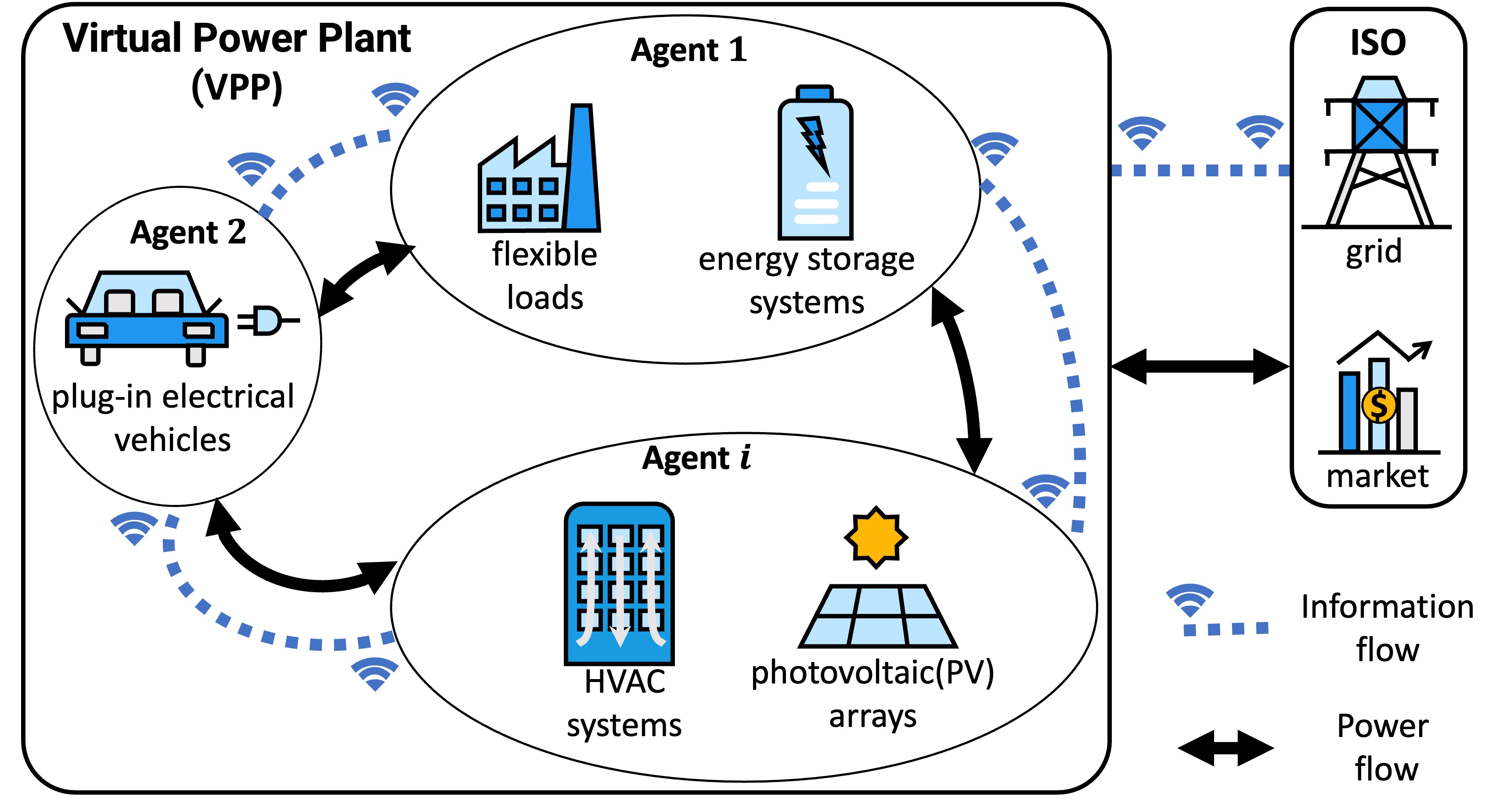
Figure 1: Examples of agents controlled by a VPP.

In this paper, we propose that the VPP operates within a two-settlement energy market, composed of a day-ahead and a real-time market. Upon the clearing of the day-ahead market, the VPP decides on hourly production schedules. The real-time market, also known as the imbalance market, is designed to settle potential day-ahead commitment violations. The real-time market productions are set in 5-minute increments. The production schedules every 5 minutes are denoted as $\mathbf{P}_{\texttt{Sch}}$.

The $\mathcal{LOOP-MAC}$  method is designed for the real-time market, where a VPP solves a dispatch optimization across its assets (agents) to honor its commitment over a given time scale, $[t_{\texttt{s}},t_{\texttt{e}}]$, where $t_{\texttt{s}}$ and $t_{\texttt{e}}$ represent the starting and ending times, respectively. Put differently, the VPP needs to fulfill the production schedule $\mathbf{P}_{\texttt{Sch}}=\left[{P}_{\texttt{Sch}}^{t}\mid t=t_{\texttt{s}},\ldots,t_{\texttt{e}}\right]$ while minimizing the overall cost of agents. Generally, the VPP implements 5-minute binding intervals ($\Delta t=5/60$ h) for the real-time market, and adopts look-ahead horizon $(t_{\texttt{e}}-t_{\texttt{s}})$, ranging from 5 minutes up to 2 hours [42], for the real-time dispatch optimization. The detailed dispatch optimization problem is presented next.

II-C Centralized Formulation of the VPP Coordination Problem

This subsection presents the centralized form of the power dispatch problem solved by a VPP over various assets for every time step $t\in[t_{\texttt{s}},t_{\texttt{e}}]$. The asset constraints are:

II-C1 Constraints Pertaining to Flexible Loads

The power of a flexible load should be within a pre-defined operation range $[P_{\texttt{FLmin}}^{i,t},P_{\texttt{FLmax}}^{i,t}]$, $\forall t\in[t_{\texttt{s}},t_{\texttt{e}}]$, $\forall i\in\mathcal{N}_{\texttt{A}}$:

$$P_{\texttt{FLmin}}^{i,t}\leq P_{\texttt{FL}}^{i,t}\leq P_{\texttt{FLmax}}^{i,t}$$ (5)

II-C2 Constraints Pertaining to Energy Storage Systems

$\forall i$ and $\forall t\in[t_{\texttt{s}},t_{\texttt{e}}]$, the charging $P_{\texttt{ESSC}}^{i,t}$ (or discharging $P_{\texttt{ESSD}}^{i,t}$) power of the energy storage system must not exceed $P_{\texttt{ESSmax}}^{i}$, as indicated in (6). Also, (7) and (8) define $R_{\texttt{SoC}}^{i,t}$ as the state of charge (SoC) and bound its limits. Here $\eta_{\texttt{ESSC}}^{i}$ and $\eta_{\texttt{ESSD}}^{i}$ denote the charging and discharging efficiency. Finally $E_{\texttt{ESSN}}^{i}$ refers to the capacity.

$$0\leq P_{\texttt{ESSC}}^{i,t} \leq P_{\texttt{ESSmax}}^{i},~{}~{}~{}0\leq P_{\texttt{ESSD}}^{i,t}\leq P_{\texttt{ESSmax}}^{i}$$ (6)

$$R_{\texttt{SoC}}^{i,t+1}= R_{\texttt{SoC}}^{i,t}+\frac{(P_{\texttt{ESSC}}^{i,t}\eta_{\texttt{ESSC}}^{i}-\frac{P_{\texttt{ESSD}}^{i,t}}{\eta_{\texttt{ESSD}}^{i}})\Delta t}{E_{\texttt{ESSN}}^{i}}$$ (7)

$$R_{\texttt{SoCmin}}^{i}\!\!\leq R_{\texttt{SoC}}^{i,t+1}\leq\!\!R_{\texttt{SoCmax}}^{i}$$ (8)

II-C3 Constraints Pertaining to Heating, Ventilation, and Air Conditioning Systems

The inverter-based heating, ventilation, and air conditioning model [43] is presented below with consumption power denoted as $P_{\texttt{HVAC}}^{i,t}$.

$$T_{\texttt{HVAC}}^{i,t+1}\!\!=\!\!\varepsilon^{i}_{\texttt{HVAC}}T_{\texttt{HVAC}}^{i,t}\!\!+\!\!(1\!\!-\!\!\varepsilon^{i}_{\texttt{HVAC}})\left(T_{\texttt{out}}^{i,t}\!\!-\!\!\frac{\eta_{\texttt{HVAC}}^{i}}{A_{\texttt{HVAC}}^{i}}P_{\texttt{HVAC}}^{i,t}\right)$$ (9)

Where $T_{\texttt{HVAC}}^{i,t}$ is the indoor temperature at time $t$, $T_{\texttt{out}}^{i,t}$ is the forecasted outdoor temperature, $\varepsilon^{i}_{\texttt{HVAC}}$ is the factor of inertia, $\eta_{\texttt{HVAC}}^{i}$ is the coefficient of performance, $A_{\texttt{HVAC}}^{i}$ is thermal conductivity. Equation (10) introduces the concept of adaptive comfort model $[T^{i}_{\texttt{min}},T^{i}_{\texttt{max}}]$. Equation (11) enforces the control range within the size of air-conditioning $P^{i}_{\texttt{HVACmax}}$.

$$T^{i}_{\texttt{min}}\leq T_{\texttt{HVAC}}^{i,t+1}\leq T^{i}_{\texttt{max}}$$ (10)

$$0\leq P_{\texttt{HVAC}}^{i,t}\leq P^{i}_{\texttt{HVACmax}}$$ (11)

II-C4 Constraints Pertaining to Plug-in Electric Vehicles

$\forall i$ and $\forall t\in[t_{\texttt{s}},t_{\texttt{e}}]$, the plug-in electric vehicles charging power $P_{\texttt{PEV}}^{i,t}$ must adhere to the range $[P_{\texttt{PEVmin}}^{i},P_{\texttt{PEVmax}}^{i}]$ as described in (12). Further, (13) mandates that agent $i$’s cumulative charging power meet the necessary energy $E_{\texttt{PEV}}^{i}$ for daily commute [44].

$$P_{\texttt{PEVmin}}^{i}\leq P_{\texttt{PEV}}^{i,t}\leq P_{\texttt{PEVmax}}^{i}$$ (12)

$$\sum_{t=t_{\texttt{s}}}^{t_{\texttt{e}}}P_{\texttt{PEV}}^{i,t}\geq E_{\texttt{PEV}}^{i}$$ (13)

II-C5 Constraints Pertaining to Photovoltaic Arrays

The photovoltaic power generation, given by (14) and is determined by the solar irradiance-power conversion function. Here, $R_{\texttt{PV}}^{t}$, represents the solar radiation intensity, $A_{\texttt{PV}}$ denotes the surface area, and $\eta_{\texttt{PV}}$ is the transformation efficiency.

$$P_{\texttt{PV}}^{i,t}=R_{\texttt{PV}}^{t}A_{\texttt{PV}}\eta_{\texttt{PV}}$$ (14)

II-C6 Constraints of Network Sharing

The net power of agent $i$, $P_{\texttt{O}}^{i,t}$, is given below. Note, $P_{\texttt{IL}}^{i,t}$ indicates the inflexible loads.

$$P_{\texttt{O}}^{i,t}\!\!=\!\!P_{\texttt{PV}}^{i,t}+ P_{\texttt{ESSD}}^{i,t}\!\!-\!\!P_{\texttt{ESSC}}^{i,t}\!\!-\!\!P_{\texttt{IL}}^{i,t}\!\!-\!\!P_{\texttt{FL}}^{i,t}\!\!-\!\!P_{\texttt{HVAC}}^{i,t}\!\!-\!\!P_{\texttt{PEV}}^{i,t}$$ (15)

Local distribution utility constraints are enforced by (16), while (17) guarantees that VPP’s output honors the production schedule of both energy markets.

$$P_{\texttt{Omin}}^{i}\leq P_{\texttt{O}}^{i,t}\leq P_{\texttt{Omax}}^{i}$$ (16)

$$\sum_{i\in\mathcal{N}_{\texttt{A}}}P_{\texttt{O}}^{i,t}=P_{\texttt{Sch}}^{t}$$ (17)

II-C7 Objective Function

The objective function for the power dispatch problem, given by (18), and comprises the following terms:

Minimizing maintenance and operation costs of energy storage systems

$\alpha_{\texttt{ESS}}^{i}$ represents the unit maintenance cost.

Balancing the differences between actual and preset consumption profiles for flexible loads

$\alpha_{\texttt{FL}}^{i,t}$ is the inconvenience coefficient. Here, $P_{\texttt{FLref}}^{i,t}$ specifies the preferred consumption level [45].

Mitigating thermal discomfort costs for HVAC systems

$\alpha_{\texttt{HVAC}}^{i,t}$ is the cost coefficient, $T_{\texttt{Ref}}^{i,t}$ indicates the optimal comfort level, and binary variable $\beta_{\texttt{HVAC}}^{i,t}$ denotes occupancy state, where 1 means occupied and 0 indicates vacancy.

$$f=\sum_{t=t_{\texttt{s}}}^{t_{\texttt{e}}}\sum_{i\in\mathcal{N}_{\texttt{A}}}\left(\alpha_{\texttt{ESS}}^{i}(P_{\texttt{ESSC}}^{i,t}+P_{\texttt{ESSD}}^{i,t})+\alpha_{\texttt{FL}}^{i}(P_{\texttt{FL}}^{i,t}\right.$$

$$\left.-P_{\texttt{FLref}}^{i,t})^{2}+\beta_{\texttt{HVAC}}^{i,t}\alpha_{\texttt{HVAC}}^{i}{(T_{\texttt{HVAC}}^{i,t}-T_{\texttt{Ref}}^{{i,t}})}^{2}\right)$$ (18)

II-C8 Centralized Optimization Problem

Combining the constraints (5)-(17) and the objective function (18), we formulate the power dispatch problem. Note the formulated dispatch problem requires frequent resolution at each time instance $t_{\texttt{s}}$ in the real-time market. For a given agent $i$, the optimization variables over the time interval $[t_{\texttt{s}},t_{\texttt{e}}]$ are denoted by $\mathbf{u}^{i}(t)$, while its inputs over the same interval are represented as $\mathbf{x}^{i}$;

$$\mathbf{u}^{i}={\left[P_{\texttt{FL}}^{i,t},P_{\texttt{ESSC}}^{i,t},P_{\texttt{ESSD}}^{i,t},R_{\texttt{SoC}}^{i,t+1},P_{\texttt{HVAC}}^{i,t},T_{\texttt{HVAC}}^{i,t+1},P_{\texttt{PEV}}^{i,t},P_{\texttt{PV}}^{i,t},\right.}$$

$${\left.P_{\texttt{O}}^{i,t}\mid t=t_{\texttt{s}},\ldots,t_{\texttt{e}}\right]}$$ (19)

$$\mathbf{x}^{i}={\left[P_{\texttt{FLmin}}^{i,t},P_{\texttt{FLmax}}^{i,t},R_{\texttt{SoC}}^{i,t_{\texttt{s}}},T_{\texttt{HVAC}}^{i,t_{\texttt{s}}},T_{\texttt{out}}^{i,t},E_{\texttt{PEV}}^{i},R_{\texttt{PV}}^{t},P_{\texttt{IL}}^{i,t},\right.}$$

$${\left.P_{\texttt{Sch}}^{t},P_{\texttt{FLref}}^{i,t},\beta_{\texttt{HVAC}}^{i,t},T_{\texttt{Ref}}^{i,t}\mid t=t_{\texttt{s}},\ldots,t_{\texttt{e}}\right]}$$ (20)

Let $\mathbf{u}=\bigoplus_{i}\mathbf{u}^{i}$ and $\mathbf{x}=\bigoplus_{i}\mathbf{x}^{i}$. The DER coordination problem can be formulated as (21) or as follows,

$$\min f(\mathbf{u},\mathbf{x})$$ (21a)

s.t. $$\mathbf{A}_{\texttt{eq}}\mathbf{u}+\mathbf{B}_{\texttt{eq}}\mathbf{x}+\mathbf{b}_{\texttt{eq}}=\mathbf{0}$$ (21b)

$$\mathbf{A}_{\texttt{ineq}}\mathbf{u}+\mathbf{B}_{\texttt{ineq}}\mathbf{x}+\mathbf{b}_{\texttt{ineq}}\leq\mathbf{0}$$ (21c)

where $\mathbf{A}_{\texttt{eq}}$, $\mathbf{B}_{\texttt{eq}}$ and $\mathbf{b}_{\texttt{eq}}$ represent the compact form of parameters in equations (7), (9), (14), (15), and (17) we have formed before. And $\mathbf{A}_{\texttt{ineq}}$, $\mathbf{B}_{\texttt{ineq}}$ and $\mathbf{b}_{\texttt{ineq}}$ captures parameters in equations (5), (6), (8), (10)-(13), (16).

II-D Agent-based Model for the VPP Coordination Problem

Agent-based problem-solving lends itself well to addressing the computational needs of the VPP coordination problem. In this subsection, we focus on finding a distributed solution for (21) (or (1)). While each sub-problem optimizes the operation of individual agents, communication enables individual agents to collectively find the system-level optimal solution.

In the context of distributed problem-solving, it is important to point out the unique challenges posed by coupling constraints such as (17). These constraints introduce intricate relationships among several agents where some variables of agent $i$ are tied with those of agent $j$. These coupled constraints prevent separating (21) into disjointed sub-problems.

As discussed in Section IIA, we define the variables present among multiple agents’ constraints as global variables, $\mathbf{u}^{i}_{\texttt{g}}$,

$$\mathbf{u}^{i}_{\texttt{g}}={\left[P_{\texttt{O}}^{i,t}\mid t=t_{\texttt{s}},\ldots,t_{\texttt{e}}\right]}^{\texttt{T}}$$ (22)

In contrast, the variables solely managed by non-overlapping constraints are referred to as local variables. That is, $\mathbf{u}^{i}=[\mathbf{u}^{i}_{\texttt{l}},\mathbf{u}^{i}_{\texttt{g}}]$. We refer to agents whose variables are intertwined in a constraint as neighboring agents.

The ADMM method finds a decentralized solution for (21) by creating local copies of neighboring agents’ global variables and adjusting local copies iteratively to satisfy both local and consensus constraints. The adjustment continues until alignment with original global variables is achieved, at which point the global minimum has been found in a decentralized manner.

In the power dispatch problem, we introduce $P_{\texttt{OCopy}}^{i,j,t}$, which is owned by agent $i$, and represents a copy of $P_{\texttt{O}}^{j,t}$. Then, coupled constraint (17) become a local constraint (23) and a consensus constraint (24):

$$P_{\texttt{O}}^{i,t}+\sum_{j\neq i}P_{\texttt{OCopy}}^{i,j,t}=P_{\texttt{Sch}}^{t}$$ (23)

$$P_{\texttt{OCopy}}^{i,j,t}=P_{\texttt{O}}^{j,t},\forall j\neq i$$ (24)

Let $\mathbf{u}^{i}_{\texttt{g,Copy}}={[P_{\texttt{OCopy}}^{i,j,t}\mid t=t_{\texttt{s}},\ldots,t_{\texttt{e}}]}$ denote all local copies owned by agent $i$ imitating other neighboring agents’ global variables. Then, one could reformulate the problem (21) in accordance to $\mathbf{u}^{i}$ and $\mathbf{u}^{i}_{\texttt{g,Copy}}$ as,

$$\min\sum_{i}f^{i}(\mathbf{u}^{i},\mathbf{u}^{i}_{\texttt{g,Copy}},\mathbf{x}^{i})$$ (25a)

$$\texttt{s.t.}~{}~{}~{}\mathbf{A}^{i}_{\texttt{eq}}\begin{bmatrix}\mathbf{u}^{i}\\ \mathbf{u}^{i}_{\texttt{g,Copy}}\end{bmatrix}+\mathbf{B}^{i}_{\texttt{eq}}\mathbf{x}^{i}+\mathbf{b}^{i}_{\texttt{eq}}=\mathbf{0},\forall i$$ (25b)

$$\mathbf{A}^{i}_{\texttt{ineq}}\begin{bmatrix}\mathbf{u}^{i}\\ \mathbf{u}^{i}_{\texttt{g,Copy}}\end{bmatrix}+\mathbf{B}^{i}_{\texttt{ineq}}\mathbf{x}^{i}+\mathbf{b}^{i}_{\texttt{ineq}}\leq\mathbf{0},\forall i$$ (25c)

$$\mathbf{u}^{i}_{\texttt{g,Copy}}=\mathbf{I}_{\texttt{c}}^{i}[\bigoplus_{j\neq i}\mathbf{u}_{\texttt{g}}^{j}],\forall i$$ (25d)

where, $\mathbf{A}^{i}_{\texttt{eq}}$, $\mathbf{B}^{i}_{\texttt{eq}}$, $\mathbf{b}^{i}_{\texttt{eq}}$, $\mathbf{A}^{i}_{\texttt{ineq}}$, $\mathbf{B}^{i}_{\texttt{ineq}}$, and $\mathbf{b}^{i}_{\texttt{ineq}}$ in (25b) and (25c) capture the compact form of constraints (5)-(16), (23). And (25d) is the compact form of constraints (24). Here $\mathbf{I}_{\texttt{c}}^{i}$ is the element selector matrix that maps elements from vector $\bigoplus_{j\neq i}\mathbf{u}_{\texttt{g}}^{j}$ to vector $\mathbf{u}^{i}_{\texttt{g,Copy}}$ based on a consensus constraint (24). Each row of $\mathbf{I}_{\texttt{c}}^{i}$ contains a single 1 at a position that corresponds to the desired element from $\bigoplus_{j\neq i}\mathbf{u}_{\texttt{g}}^{j}$ and 0s elsewhere. Therefore, $\mathbf{I}_{\texttt{c}}^{i}[\bigoplus_{j\neq i}\mathbf{u}_{\texttt{g}}^{j}]$ represents the vector of global variables that are required to be imitated by agent $i$.

Let $\mathcal{S}_{\texttt{Local}}^{i}$ be the set of local constraints associated with agent $i$, i.e., (25b)-(25c). Therefore, the compact form of decentralized formulation at the agent-level as defined in (2).

II-E Updating Rules Within Agents

The standard form of ADMM solves problem (25) (or (2)) by dealing with the augmented Lagrangian function $\mathrm{L}$:

$$\min\mathrm{L}\!\!=\!\!\! \sum_{i}\!\!\left(f^{i}(\mathbf{u}^{i},\mathbf{u}^{i}_{\texttt{g,Copy}},\mathbf{x}^{i})\!\!+\!\!{\boldsymbol{\lambda}}^{i\texttt{T}}(\mathbf{u}^{i}_{\texttt{g,Copy}}\!\!\!\!-\!\!\mathbf{I}^{i}_{\texttt{c}}[\bigoplus_{j\neq i}\mathbf{u}_{\texttt{g}}^{j}])\right.$$

$$\left.+\rho\left\|\mathbf{u}^{i}_{\texttt{g,Copy}}-\mathbf{I}_{\texttt{c}}^{i}[\bigoplus_{j\neq i}\mathbf{u}^{j}]\right\|_{2}^{2}\right)$$ (26a)

$$\begin{bmatrix}\mathbf{u}^{i}\\ \mathbf{u}^{i}_{\texttt{g,Copy}}\end{bmatrix}\in\mathcal{S}_{\texttt{Local}}^{i}(\mathbf{x}^{i}),\forall i$$ (26b)

where $\rho>0$ is a positive constant. $\boldsymbol{\lambda}^{i}$ denotes the vector of all Lagrangian multipliers for the corresponding consensus equality relationship between agent $i$’s copy and neighboring agent $j$’s global variable.

The search for a solution to (26) is performed through an iterative process (indexed by $[k],k=1,...,N_{\texttt{K}}$). All $N_{\texttt{A}}$ agents will execute this process simultaneously and independently before communicating with neighboring agents. At the agent level, these updates manifest themselves as follows,

$$\boldsymbol{\lambda}^{i^{[k]}}=\boldsymbol{\lambda}^{i^{[k-1]}}+\rho(\mathbf{u}^{i^{[k-1]}}_{\texttt{g,Copy}}-\mathbf{I}_{\texttt{c}}^{i}[\bigoplus_{j\neq i}\mathbf{u}_{\texttt{g}}^{j^{[k-1]}}])$$ (27)

$$\begin{bmatrix}\!\!\!\!\mathbf{u}^{i^{[k]}}\\ \mathbf{u}^{i^{[k]}}_{\texttt{g,Copy}}\!\!\end{bmatrix}\!\!\!=\!\!\arg\min\mathrm{L}\!\!\left(\!\!\boldsymbol{\lambda}^{i^{[k]}}\!\!\!,\bigoplus_{j\neq i}\!\!\left(\mathbf{u}^{j^{[k-1]}}\!\!\!,\mathbf{u}^{j^{[k-1]}}_{\texttt{g,Copy}},\boldsymbol{\lambda}^{j^{[k]}}\right)\!\!\!\right)\!\!,$$

$$\texttt{s.t.}\begin{bmatrix}\mathbf{u}^{i^{[k]}}\\ \mathbf{u}^{i^{[k]}}_{\texttt{g,Copy}}\end{bmatrix}\in\mathcal{S}_{\texttt{Local}}^{i}(\mathbf{x}^{i})$$ (28)

The dual update equation, given by (27), modifies the Lagrangian multipliers to estimate the discrepancies between an agent’s local copy of variables (designed to emulate the global variables of its neighbors) and the actual global variables held by those neighbors. Subsequently, (28) provides an optimization solution leveraging prior iteration data from other agents.

It’s essential to note that agent $i$ doesn’t require all the updated values from other agents to update equations (27) and (28). Agent $i$ primarily needs:

• Neighboring agents’ global variables: $\mathbf{I}_{\texttt{c}}^{i}[\bigoplus_{j\neq i}\mathbf{u}_{\texttt{g}}^{j}]$. In the context of the distributed DER problem, agent $i$ requires values of $P_{\texttt{O}}^{j,t^{[k-1]}}$ from their neighboring agent $j$.

• Neighboring agents’ local copies mirroring agent $i$’s global variables: $\mathbf{I}_{\texttt{g}}^{i}[\bigoplus_{j\neq i}\mathbf{u}_{\texttt{g,Copy}}^{j^{[k-1]}}]$, where $\mathbf{I}_{\texttt{g}}^{i}$ functions as a selector matrix. In the distributed DER context, agent $i$ requires $P_{\texttt{OCopy}}^{{j,i,t}^{[k]}}$ from their neighboring agent $j$.

We use $\mathbf{u}^{i^{[k-1]}}_{\texttt{Other}}$ to represent the set of variables owned by other agents but are needed by agent $i$ to update (27) and (28). Finally, the intra-agent updates are represented by (4) and (3).

The standard form of ADMM guarantees the feasibility of local constraints by (4) and penalizes violations of consensus constraints by iteratively updating Lagrangian multipliers as (3). In what follows, we will propose a ML-based method to accelerate ADMM for decentralized DER coordination. The ADMM iterations will guide the consensus protocol, while the gauge map [41] is adopted to enforce hard local constraints.

III Proposed $\mathcal{LOOP-MAC}$  Methodology

III-A Overview of the Method

This section provides a high-level overview of the $\mathcal{LOOP-MAC}$  method to incorporate ML to accelerate the ADMM algorithm. As shown in Fig. 2, instead of solving agent-level local optimization problems (4) by an iterative solver, we will train ${N}_{\texttt{A}}$ agent-level neural approximators $\xi^{i},i\in\mathcal{N}_{\texttt{A}}$ to directly map inputs to optimized value of agent’s optimization variables in a single feed-forward. The resulting prediction of each agent $i$, denoted as $\mathbf{u}^{i^{[k]}}$, will be trained to approximate the optimal solution of (2).

$$\mathbf{u}^{i^{[k]}},\mathbf{u}^{i^{[k]}}_{\texttt{g,Copy}}=\xi^{i}\left(\mathbf{x}^{i},\mathbf{u}^{i^{[k-1]}}_{\texttt{Other}}\right)$$ (29)

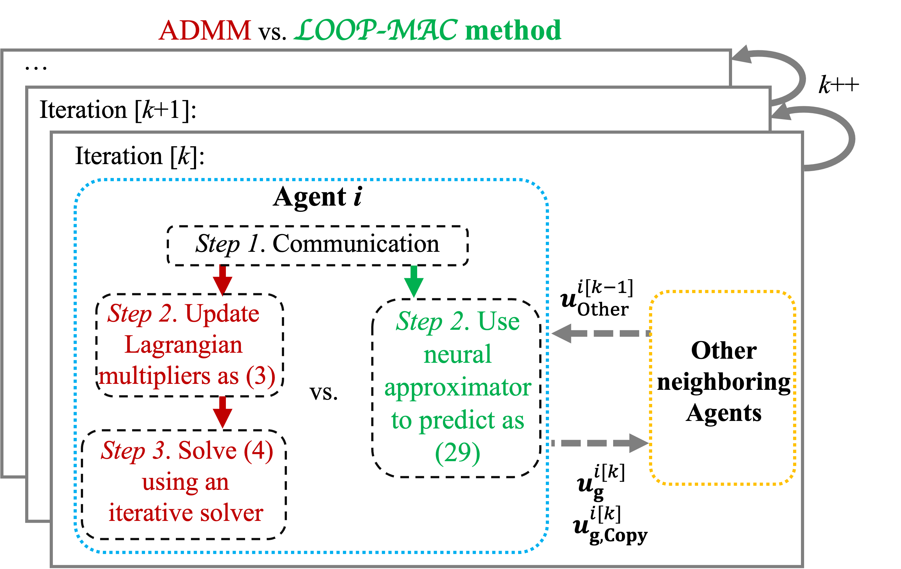
Figure 2: Comparison between ADMM and the proposed $\mathcal{LOOP-MAC}$  method. The ADMM approach is comprised of two key components: the dual update and the primal optimization. The dual update guides the consensus protocol, while the primal optimization leverages this estimation to adjust the local decision-making process through iterative solvers. In contrast, our $\mathcal{LOOP-MAC}$  method replaces these two procedures with a single-step data infusion and mapping input parameters and other agents’ values to agent-level optimized values, directly.

Pseudo code of the proposed $\mathcal{LOOP-MAC}$  method is given in Algorithm 1. $\mathcal{LOOP-MAC}$  method includes two steps for each iteration. First, each agent receives variables of prior iteration from neighboring agents. Second, each agent uses a neural approximator to predict its optimal values.

Algorithm 1 $\mathcal{LOOP-MAC}$  method

Input: DER coordination problem parameters, e.g., ${N}_{\texttt{A}}$ neural approximators $\xi^{i},\forall i$, input parameters $\mathbf{x}^{i},\forall i$; Initial value of $\mathbf{u}^{i}$ and $\boldsymbol{\lambda}^{i},\forall i$.

Output: Distributed solution $\mathbf{u}^{i^{[k+1]}}$ to DER coordination problem.

while Convergence criteria unmet do

     for $i$ in range($\mathcal{N}_{\texttt{A}}$) do

         $\bullet$ Send previous global variable $\mathbf{u}^{i^{[k-1]}}_{\texttt{g}}$ and local copy $\mathbf{u}^{i^{[k-1]}}_{\texttt{g,Copy}}$ to neighboring agents, and receive $\mathbf{u}^{i^{[k-1]}}_{\texttt{Other}}$

         $\bullet$ Generate prediction $\mathbf{u}^{i^{[k]}},\mathbf{u}^{i^{[k]}}_{\texttt{g,Copy}}\!=\!\xi^{i}(\mathbf{x}^{i},\mathbf{u}^{i^{[k-1]}}_{\texttt{Other}})$

         $k++$

     end for

end while

III-B Design of Neural Approximators Structures

Violations of consensus constraints could be penalized by ADMM iterations. Further, we will design each neural approximator’s structure to guarantee that its output satisfies the local constraints, i.e., $\xi^{i}\in\mathcal{S}_{\texttt{Local}}^{i}(\mathbf{x}^{i})$. We adopt the $\mathcal{LOOP-LC}$ (Learning to Optimize the Optimization Process with Linear Constraints) model proposed in [41] to develop each neural approximator $\xi^{i}$. The $\mathcal{LOOP-LC}$ model learns to solve optimization problems with hard linear constraints. It applies variable elimination and gauge mapping for equality and inequality completions, respectively. The $\mathcal{LOOP-LC}$ model produces a feasible and near-optimal solution. In what follows, we will present the main components of $\mathcal{LOOP-LC}$ and how it applies to the VPP coordination problem.

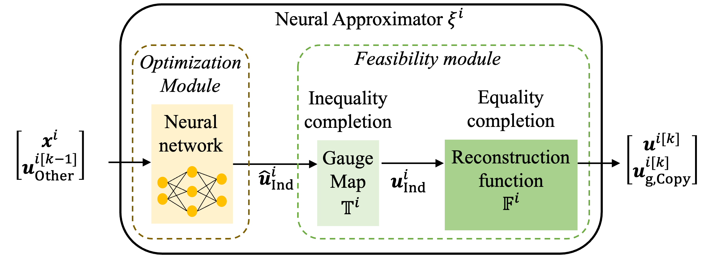
Figure 3: The structure and building blocks of Neural Approximator $\xi^{i}$.

III-B1 Variable Elimination

Based on the equality constraints given in (25b), the variables $\mathbf{u}^{i}$ and $\mathbf{u}^{i}_{\texttt{g,Copy}}$ can be categorized into two sets: the dependent variables $\mathbf{u}^{i}_{\texttt{Dep}}$ and the independent variables $\mathbf{u}^{i}_{\texttt{Ind}}$. The dependent variables are inherently determined by the independent variables. For instance in (9), the variable $T_{\texttt{HVAC}}^{i,t+1}$ is dependent on $P_{\texttt{HVAC}}^{i,t}$; hence, once $P_{\texttt{HVAC}}^{i,t}$ is derived, $T_{\texttt{HVAC}}^{i,t+1}$ can be caculated.

The function $\mathbb{F}^{i}$ is introduced to establish the relationship between $\mathbf{u}^{i}_{\texttt{Dep}}$ and $\mathbf{u}^{i}_{\texttt{Ind}}$, such that $\mathbf{u}^{i}_{\texttt{Dep}}=\mathbb{F}^{i}(\mathbf{u}^{i}_{\texttt{Ind}})$, shown in Fig. 3. A comprehensive derivation of $\mathbb{F}^{i}$ can be found in [41]. By integrating $\mathbb{F}^{i}$ into the definition of $\mathcal{S}_{\texttt{Local}}^{i}$ and substituting $\mathbf{u}^{i}_{\texttt{Dep}}$, the optimization problem of (4) can be restructured as a reduced-dimensional problem with $\mathbf{u}^{i}_{\texttt{Ind}}$ as the primary variable. The corresponding constraint set for this reformulated problem is denoted by $\mathcal{S}_{\texttt{Local,Ref}}^{i}$ and presented as,

$$\mathcal{S}_{\texttt{Local,Ref}}^{i}=\begin{Bmatrix}\mathbf{A}^{i}_{\texttt{ineq}}\begin{bmatrix}\mathbf{u}^{i}_{\texttt{Ind}}\\ \mathbb{F}^{i}(\mathbf{u}^{i}_{\texttt{Ind}})\end{bmatrix}+\mathbf{B}^{i}_{\texttt{ineq}}\mathbf{x}^{i}+\mathbf{b}^{i}_{\texttt{ineq}}\leq\mathbf{0}\end{Bmatrix}$$ (30)

Therefore, as long as the prediction of the reformulated problem ensures $\mathbf{u}^{i}_{\texttt{Ind}}\in\mathcal{S}_{\texttt{Local,Ref}}^{i}$, $\mathbb{F}^{i}$ will produce the full-size $\mathbf{u}^{i},\mathbf{u}^{i}_{\texttt{g,Copy}}$ vectors satisfying local constraints $\mathcal{S}_{\texttt{Local}}^{i}(\mathbf{x}^{i})$ by concatenating $\mathbf{u}^{i}_{\texttt{Dep}}$ and $\mathbf{u}^{i}_{\texttt{Dep}},\mathbf{u}^{i}_{\texttt{Ind}}$.

III-B2 Gauge Map

After variable elimination, our primary objective is to predict $\mathbf{u}^{i}_{\texttt{Ind}}$ such that it satisfies the constraint set $\mathcal{S}_{\texttt{Local,Ref}}^{i}$. Instead of directly solving this problem, we will utilize a neural network that finds a virtual prediction $\mathbf{\hat{u}}^{i}_{\texttt{Ind}}$ which lies within the $\ell_{\infty}$-norm unit ball (denoted as $\mathcal{B}$) a set constrained by upper and lower bounds. The architecture of the neural network is designed to ensure that the resulting $\mathbf{\hat{u}}^{i}_{\texttt{Ind}}$ remains confined within $\mathcal{B}$. Subsequently, we introduce a bijective gauge mapping, represented as $\mathbb{T}^{i}$, to transform $\mathbf{\hat{u}}^{i}_{\texttt{Ind}}$ from $\mathcal{B}$ to $\mathcal{S}_{\texttt{Local,Ref}}^{i}$. As presented in [41], $\mathbb{T}^{i}$ is a predefined function with an explicit closed-form representation as below,

$$\mathbf{u}^{i}_{\texttt{Ind}}=\mathbb{T}^{i}(\mathbf{\hat{u}}^{i}_{\texttt{Ind}})=\frac{\psi_{\mathcal{B}}(\mathbf{\hat{u}}^{i}_{\texttt{Ind}})}{\psi_{\mathcal{S}_{\texttt{Local,Ref0}}^{i}}(\mathbf{\hat{u}}^{i}_{\texttt{Ind}})}\mathbf{\hat{u}}^{i}_{\texttt{Ind}}+\mathbf{u}^{i}_{\texttt{Ind,0}}$$ (31)

The function $\psi_{\mathcal{B}}$ is the Minkowski gauge of the set $\mathcal{B}$, while $\mathbf{u}^{i}_{\texttt{Ind,0}}$ represents an interior point of $\mathcal{S}_{\texttt{Local,Ref}}^{i}$. Moreover, the shifted set, $\mathcal{S}_{\texttt{Local,Ref0}}^{i}$, is defined as,

$$\mathcal{S}_{\texttt{Local,Ref0}}^{i}=\left\{\mathbf{\bar{u}}^{i}_{\texttt{Ind}}\mid\left(\mathbf{u}^{i}_{\texttt{Ind,0}}+\mathbf{\bar{u}}^{i}_{\texttt{Ind}}\right)\in\mathcal{S}_{\texttt{Local,Ref}}^{i}\right\}$$ (32)

with $\psi_{\mathcal{S}_{\texttt{Local,Ref0}}^{i}}$ representing the Minkowski gauge on this set.

III-C Training the Neural Approximators

We use the historical trajectories of ADMM (i.e. applied on historical power demands) for training purposes. Note that predicting the converged ADMM values is a time-series prediction challenge. Specifically, outputs from a given iteration are requisites for the subsequent iterations. This relationship implies that $\mathbf{u}^{i^{[k]}},\mathbf{u}^{i^{[k]}}_{\texttt{g,Copy}},\forall i$ are contingent upon $\mathbf{u}^{i^{[k-1]}}_{\texttt{Other}}$, derived from other agents’ outputs $\mathbf{u}^{j^{[k-1]}},\mathbf{u}^{j^{[k-1]}}_{\texttt{g,Copy}},\forall j\neq i$ from the prior iteration. To encapsulate this temporal dependency, our training approach adopts a look-ahead format, facilitating the joint training of all neural approximators in a recurrent manner, which ensures that prior outputs from different agents are seamlessly integrated as current inputs (see Fig. 4).

Suppose there are $N_{\texttt{D}}$ training data points, indexed and associated with their respective output by the superscript $(d)$. As an initial step, ADMM is employed to generate all values of optimization variables required for training. Concurrently, the optimal solution $\mathbf{u}^{i*(d)}$ pertaining to (2) is calculated. Subsequently, for $N_{\texttt{R}}$ recurrent steps, the loss function $f_{\texttt{L}}$ is defined as the cumulative distance $d$ between the prediction $\mathbf{u}^{i^{[k+r](d)}}$ and the optimal solution $\mathbf{u}^{i*(d)}$. This summation spans all agents, every recurrent step, every iteration ($k=1,..N_{\texttt{K}}$), and all data points, as delineated in (33).

$$f_{\texttt{L}}=\sum_{d=1}^{N_{\texttt{D}}}\sum_{k=1}^{N_{\texttt{K}}}\sum_{r=1}^{N_{\texttt{R}}}\sum_{i\in\mathcal{N}_{\texttt{A}}}d(\mathbf{u}^{i^{[k+r](d)}},\mathbf{u}^{i*(d)})$$ (33)

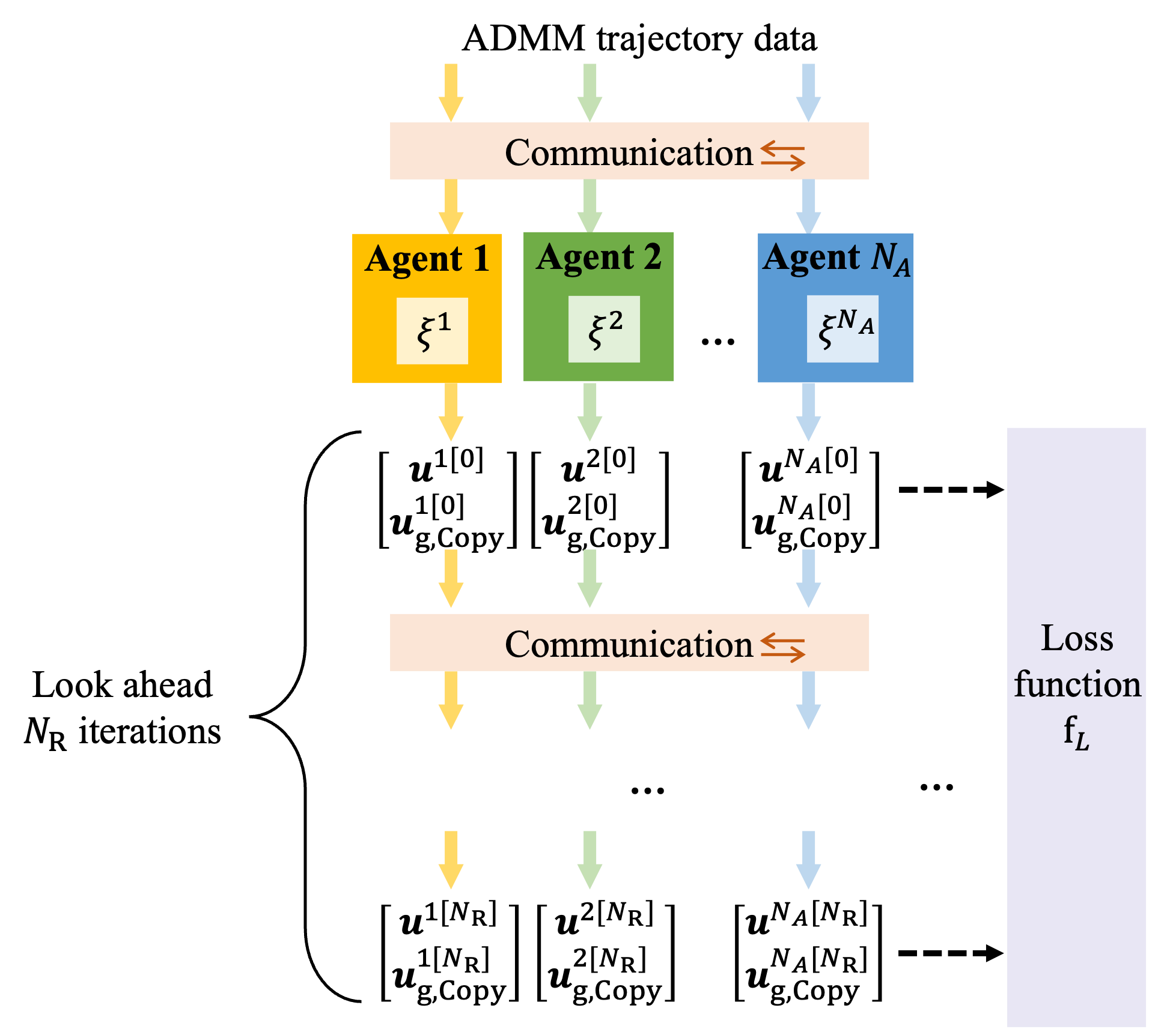
Figure 4: ADMM convergence values present a time-series prediction challenge, with outputs from one iteration feeding into the next. Our training approach uses a look-ahead format, enabling recurrent joint training of neural approximators, integrating prior outputs as current inputs.

IV Experimental Results

IV-A Experiment Setup

IV-A1 Test Systems

We examine a VPP consisting of three distinct agents, as illustrated in Fig. 5.

• Agent 1 manages inflexible loads, flexible loads, and energy storage systems.

• Agent 2 is responsible for inflexible loads and the operations of plug-in electric vehicles.

• Agent 3 oversees inflexible loads, heating, ventilation, and air conditioning systems, in addition to photovoltaics.

We derive the load profile from data recorded in the central area of New York on July 24th, 2023 [46]. Both preferred flexible loads and inflexible loads typically range between 10 kW and 25 kW. The production schedule range is set between 45 kW and 115 kW.

For plug-in electric vehicles, our reference is the average hourly public L2 charging station utilization on weekdays in March 2022 as presented by Borlaug et al. [47]. In [47] the profile range for $E_{\texttt{PEV}}^{i,\tau},\tau\in[0,24h]$ between 10 and 22 kW.

With regards to the heating, ventilation, and air conditioning systems, the target indoor temperature $T_{\texttt{Ref}}^{i,t}$ is maintained at ${77}^{\circ}F$. Guided by the ASHRAE(American Society of Heating, Refrigerating, and Air-Conditioning Engineers) standards [48], the acceptable summer comfort range is determined as $T^{i}_{\texttt{min}}={75}^{\circ}F$ and $T^{i}_{\texttt{max}}={79}^{\circ}F$. External temperature readings for New York City’s Central Park on July 24th, 2023 were obtained from the National Weather Service [49].

Concerning photovoltaic arrays, the Global CMP22 dataset from July 24th, 2023 [50] is used to calculate the regional solar radiation intensity $R_{\texttt{PV}}^{t}$. Supplementary parameter specifics are showcased in Table I.

IV-A2 Training Data

A total of 20 ADMM iterations are considered, i.e., $N_{\texttt{K}}=20$. This results in a dataset of $24\times 12\times 20$ data points. For model validation, data from odd time steps is designated for training, whereas even time steps are reserved for testing. The DER coordination problem includes 192 optimization variables alongside 111 input variables.

IV-A3 ADMM Configuration

The ADMM initialization values are set to zero. In our ADMM implementation, the parameter $\rho$ is set to $0.0005$. Optimization computations are carried out using the widely-accepted commercial solver, Gurobi [51].

IV-A4 Neural Network Configuration

Our neural network models consist of a single hidden layer, incorporating 500 hidden units. The Rectified Linear Unit (ReLU) activation function is employed for introducing non-linearity. To ensure that $\mathbf{\hat{u}}^{i}_{\texttt{Ind}}$ resides within $\mathcal{B}$ (the $\ell_{\infty}$ unit ball), the output layer utilizes the Hyperbolic Tangent (TanH) activation. Furthermore, 3 recurrent steps are considered, represented by $N_{\texttt{R}}=3$.

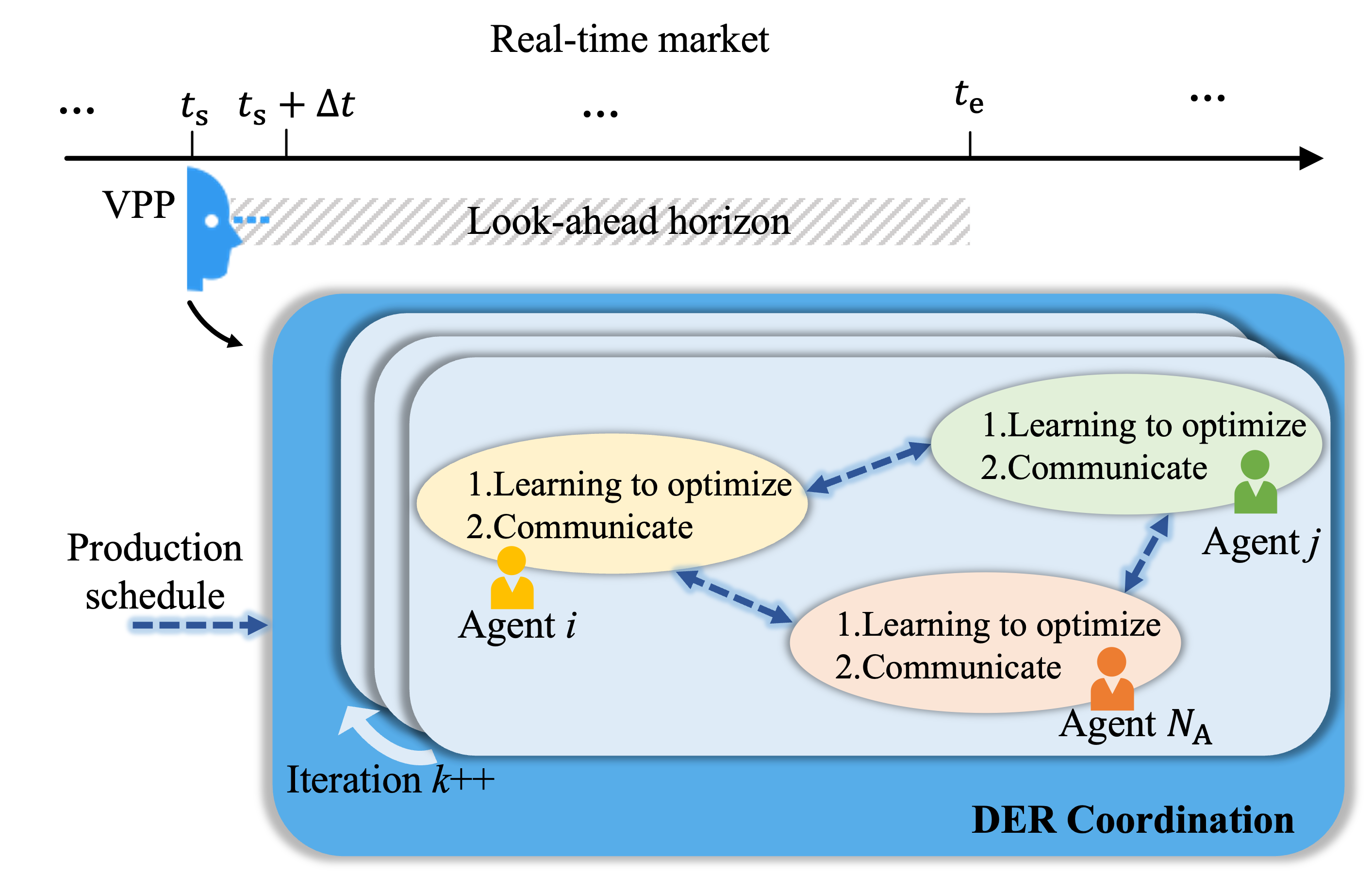
Figure 5: Applying the proposed $\mathcal{LOOP-MAC}$  method to the DER coordination problem within VPPs.

TABLE I: Parameters of DERs that are controlled by agents.

parameter	value	parameter	value
$\alpha_{\texttt{FL}}^{i,t}$	0.1 [45]	$P_{\texttt{ESSmax}}^{i}$	80kW [45]
$\alpha_{\texttt{ESS}}^{i}$	0.01 [52]	$\eta_{\texttt{ESSC}}^{i}$	0.94 [45]
$\eta_{\texttt{ESSD}}^{i}$	1.06 [45]	$E_{\texttt{ESSN}}^{i}$	300kW [45]
$R_{\texttt{SoCmin}}^{i}$	0.15 [45]	$R_{\texttt{SoCmax}}^{i}$	0.85 [45]
$R_{\texttt{SoC}}^{i}(\tau=0)$	0.2 [45]	$\alpha_{\texttt{ESS}}^{i}$	0.01 [52]
$\eta_{\texttt{HVAC}}^{i}$	2.5 [43]	$A_{\texttt{HVAC}}^{i}$	0.25[43]
$\varepsilon^{i}_{\texttt{HVAC}}$	0.93 [43]	$P^{i}_{\texttt{HVACmax}}$	11.5kW [43]
$\beta_{\texttt{HVAC}}^{i,t}$	1	$\alpha_{\texttt{HVAC}}^{i,t}$	1
$A_{\texttt{PV}}$	1000 $m^{2}$ [53]	$\eta_{\texttt{PV}}$	0.2[53]

IV-B Runtime Results

Fig. 6 illustrates the cumulative computation time across all agents and test data points over iterations. The performance comparison is conducted among the decentralized setup employing ADMM solvers, our proposed $\mathcal{LOOP-MAC}$  method, and the centralized approach using traditional centralized solvers.

From the case study, it is observed that the computational time required by the classical ADMM solver exceeds the centralized solvers solution time after approximately five iterations. Remarkably, our proposed $\mathcal{LOOP-MAC}$ method significantly outperforms the classical ADMM, achieving 500x speed up. Also, $\mathcal{LOOP-MAC}$  even surpasses the efficiency of the centralized solver in terms of computation speed.

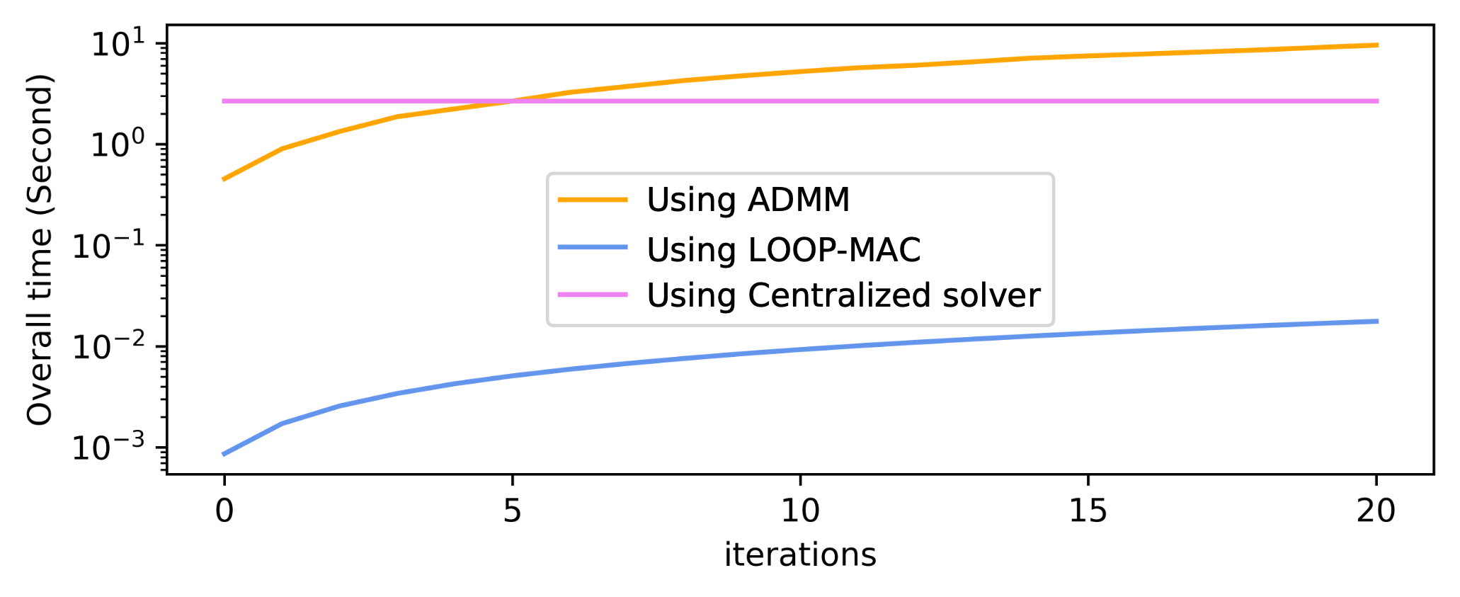
Figure 6: Comparison of cumulative computational time across all agents and test data points. The classical ADMM approach closely matches the computational efficiency of centralized solvers after approximately five iterations. In stark contrast, our proposed $\mathcal{LOOP-MAC}$  strategy achieves a speed nearly 500 times faster than the classical ADMM, even surpassing the centralized solvers in performance.

Table II provides the average computational time for a single iteration on a single data point. An insightful observation from the results suggests that the $\mathcal{LOOP-MAC}$  method would require around 3300 iterations to match the computational time of centralized solvers. However, based on the convergence analysis that will be provided later, $\mathcal{LOOP-MAC}$  method demonstrates convergence in a mere 10 iterations.

TABLE II: Average running time for a single ADMM iteration over the decision-making time horizon .

Method	Time(Millisecond)
$\mathcal{LOOP-MAC}$  method	0.0060
ADMM using Gurobi[51]	3.2966
Centralized formulation using Gurobi [51]	19.4496/$N_{\texttt{K}}$

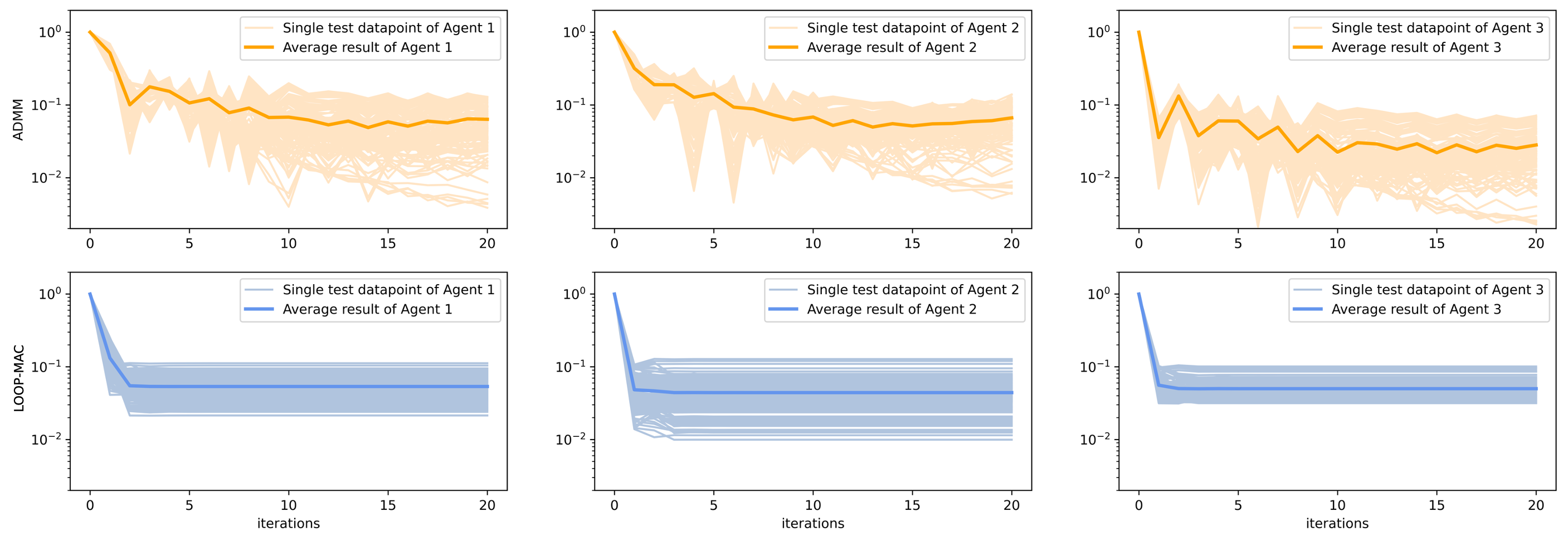
Figure 7: Comparison of the optimality deviation (error) rate for the classical ADMM versus $\mathcal{LOOP-MAC}$. The rate quantifies deviation (error) from the optimal DER operation profile using $\left\|\mathbf{u}^{i^{[k](d)}}-\mathbf{u}^{i*(d)}\right\|^{2}_{2}/\left\|\mathbf{u}^{i*(d)}\right\|^{2}_{2}$. $\mathcal{LOOP-MAC}$ method distinctly reduces the iterations needed for convergence and demonstrates decreased post-convergence variance and peak deviation, demonstrating its superior capabilities in handling repetitive optimization scenarios.

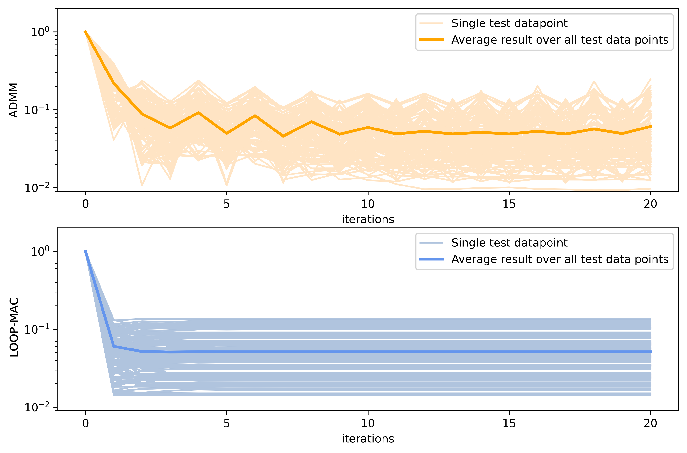
Figure 8: VPP output deviation rate represents the variance between the VPP’s output and planned production schedules, measured by the feasibility gap rate of coupled constraints (17) as $\sum_{t=\tau}^{\tau+\tau_{\texttt{w}}}\left(\sum_{i}P_{\texttt{O}}^{i,t}-P_{\texttt{Sch}}^{t}\right)/P_{\texttt{Sch}}^{t}$. Compared to the traditional ADMM, $\mathcal{LOOP-MAC}$  exhibits a faster and more stable decline towards the optimal solution.

IV-C Optimality and Feasibility Results

Fig. 7 presents the optimality deviation rate for both the traditional ADMM algorithm and $\mathcal{LOOP-MAC}$  method. The deviation rate metric quantifies the degree to which the operational profiles of the DERs deviate from the optimal (derived from solving the centralized problem). It is evident that $\mathcal{LOOP-MAC}$  method achieves faster convergence. Moreover, $\mathcal{LOOP-MAC}$  showcases faster reduction of the deviation rate compared to the standard ADMM approach.

Similarly, Fig. 8 depicts the deviation rate of the VPP schedule for both the ADMM approach and $\mathcal{LOOP-MAC}$  method. This rate sheds light on the difference between the actual VPP production schedule and its planned output. In the context of our optimization problem, the deviation rate is equivalent to the feasibility gap rate of the coupled constraints, as shown in (17). Notably, $\mathcal{LOOP-MAC}$  excels in convergence speed and stability. The VPP schedule deviation rate declines more rapidly and remains stable using $\mathcal{LOOP-MAC}$ method, whereas the traditional ADMM method results in more oscillations and converges at a slower pace.

Table III summarizes post-convergence metrics for both algorithms across all agents, iterations, and test data points. While the minimum optimality deviation rate achieved by $\mathcal{LOOP-MAC}$  is slightly higher than that of the classical ADMM, our approach showcases a much lower variance and a significantly reduced maximum deviation. These results highlight $\mathcal{LOOP-MAC}$  method’s efficacy, especially when tasked with recurrently solving similar optimization problems. The observed improvements in variance and maximum deviation highlight the versatility and robustness of $\mathcal{LOOP-MAC}$  in varied problem scenarios.

TABLE III: Post-convergence statistics.

		ADMM	$\mathcal{LOOP-MAC}$
Optimality deviation rate	Average	0.0527	0.0492
	Variance	0.0012	0.0003
	Maximum	0.1396	0.1278
	Minimum	0.0023	0.0099
VPP schedule deviation rate	Average	0.0611	0.0512
	Variance	0.0026	0.0008
	Maximum	0.2471	0.1363
	Minimum	0.0097	0.0142

To sum up, the proposed $\mathcal{LOOP-MAC}$ solution speeds up the solution time of each ADMM iteration by up to 500X. Also, $\mathcal{LOOP-MAC}$  needs fewer iterations to converge, hence, the overall run time will be significantly shorter.

V Conclusion

In this work, we introduced a novel ML-based method, $\mathcal{LOOP-MAC}$, to significantly enhance the performance of the distributed optimization techniques and discussed its performance in addressing challenges of the DER coordination problem (solved by VPP). Our multi-agent framework for VPP decision-making allows each agent to manage multiple DERs. Key to our proposed $\mathcal{LOOP-MAC}$ approach is the capability of each agent to predict their local power profiles and strategically communication with neighboring agents. The collective problem-solving efforts of these agents result in a near-optimal solution for power dispatching, ensuring compliance with both local and system-level constraints.

A key contribution of our work is developing and incorporating neural network approximators in the process of distributed decision-making. This novelty significantly accelerates the solution search and reduces the iterations required for convergence. Uniquely, in contrast to restoration-centric methodologies, $\mathcal{LOOP-MAC}$  bypasses the need for auxiliary post-processing steps to achieve feasibility using a two-pronged solution approach, where local constraints are inherently satisfied through the gauge mapping technique, and coupled constraints are penalized over ADMM iterations.

The $\mathcal{LOOP-MAC}$  method reduces the solution time per iteration by up to 500%. Coupled with requiring fewer iterations for convergence, the net result is a drastic reduction of overall convergence time while respecting the problem constraints and maintaining the quality of the resulting solution.

References

- [1] Q. Wang, C. Zhang, Y. Ding, G. Xydis, J. Wang, and J. Østergaard, “Review of real-time electricity markets for integrating distributed energy resources and demand response,” Applied Energy, vol. 138, pp. 695–706, 2015.
- [2] E. B.C. and A. Somani, “Impact of ferc order 2222 on der participation rules in us electricity markets,” tech. rep., Pacific Northwest National Laboratory, Richland, WA, 2022.
- [3] B. Goia, T. Cioara, and I. Anghel, “Virtual power plant optimization in smart grids: A narrative review,” Future Internet, vol. 14, no. 5, p. 128, 2022.
- [4] T. Navidi, A. El Gamal, and R. Rajagopal, “Coordinating distributed energy resources for reliability can significantly reduce future distribution grid upgrades and peak load,” Joule.
- [5] H. Pandžić, J. M. Morales, A. J. Conejo, and I. Kuzle, “Offering model for a virtual power plant based on stochastic programming,” Applied Energy, vol. 105, pp. 282–292, 2013.
- [6] H. Pandžić, I. Kuzle, and T. Capuder, “Virtual power plant mid-term dispatch optimization,” Applied energy, vol. 101, pp. 134–141, 2013.
- [7] E. Dall’Anese, S. S. Guggilam, A. Simonetto, Y. C. Chen, and S. V. Dhople, “Optimal regulation of virtual power plants,” IEEE transactions on power systems, vol. 33, no. 2, pp. 1868–1881, 2017.
- [8] M. Vasirani, R. Kota, R. L. Cavalcante, S. Ossowski, and N. R. Jennings, “An agent-based approach to virtual power plants of wind power generators and electric vehicles,” IEEE Transactions on Smart Grid, vol. 4, no. 3, pp. 1314–1322, 2013.
- [9] M. Mohammadi, J. Thornburg, and J. Mohammadi, “Towards an energy future with ubiquitous electric vehicles: Barriers and opportunities,” Energies, vol. 16, no. 17, p. 6379, 2023.
- [10] M. Mohammadi and A. Mohammadi, “Empowering distributed solutions in renewable energy systems and grid optimization,” in Distributed Machine Learning and Optimization: Theory and Applications, pp. 1–17, Springer, 2023.
- [11] N. Ruiz, I. Cobelo, and J. Oyarzabal, “A direct load control model for virtual power plant management,” IEEE Transactions on Power Systems, vol. 24, no. 2, pp. 959–966, 2009.
- [12] A. Bagchi, L. Goel, and P. Wang, “Adequacy assessment of generating systems incorporating storage integrated virtual power plants,” IEEE Transactions on Smart Grid, vol. 10, no. 3, pp. 3440–3451, 2018.
- [13] A. Mnatsakanyan and S. W. Kennedy, “A novel demand response model with an application for a virtual power plant,” IEEE Transactions on Smart Grid, vol. 6, no. 1, pp. 230–237, 2014.
- [14] A. Thavlov and H. W. Bindner, “Utilization of flexible demand in a virtual power plant set-up,” IEEE Transactions on Smart Grid, vol. 6, no. 2, pp. 640–647, 2014.
- [15] A. Cherukuri and J. Cortés, “Distributed coordination of ders with storage for dynamic economic dispatch,” IEEE transactions on automatic control, vol. 63, no. 3, pp. 835–842, 2017.
- [16] E. G. Kardakos, C. K. Simoglou, and A. G. Bakirtzis, “Optimal offering strategy of a virtual power plant: A stochastic bi-level approach,” IEEE Transactions on Smart Grid, vol. 7, no. 2, pp. 794–806, 2015.
- [17] M. Shabanzadeh, M.-K. Sheikh-El-Eslami, and M.-R. Haghifam, “An interactive cooperation model for neighboring virtual power plants,” Applied energy, vol. 200, pp. 273–289, 2017.
- [18] M. Giuntoli and D. Poli, “Optimized thermal and electrical scheduling of a large scale virtual power plant in the presence of energy storages,” IEEE Transactions on Smart Grid, vol. 4, no. 2, pp. 942–955, 2013.
- [19] A. G. Zamani, A. Zakariazadeh, and S. Jadid, “Day-ahead resource scheduling of a renewable energy based virtual power plant,” Applied Energy, vol. 169, pp. 324–340, 2016.
- [20] H. Wang, Y. Jia, C. S. Lai, and K. Li, “Optimal virtual power plant operational regime under reserve uncertainty,” IEEE Transactions on Smart Grid, vol. 13, no. 4, pp. 2973–2985, 2022.
- [21] S. Hadayeghparast, A. S. Farsangi, and H. Shayanfar, “Day-ahead stochastic multi-objective economic/emission operational scheduling of a large scale virtual power plant,” Energy, vol. 172, pp. 630–646, 2019.
- [22] Ö. P. Akkaş and E. Çam, “Optimal operational scheduling of a virtual power plant participating in day-ahead market with consideration of emission and battery degradation cost,” International Transactions on Electrical Energy Systems, vol. 30, no. 7, p. e12418, 2020.
- [23] S. R. Dabbagh and M. K. Sheikh-El-Eslami, “Risk assessment of virtual power plants offering in energy and reserve markets,” IEEE Transactions on Power Systems, vol. 31, no. 5, pp. 3572–3582, 2015.
- [24] G. Chen and J. Li, “A fully distributed admm-based dispatch approach for virtual power plant problems,” Applied Mathematical Modelling, vol. 58, pp. 300–312, 2018.
- [25] D. K. Molzahn, F. Dörfler, H. Sandberg, S. H. Low, S. Chakrabarti, R. Baldick, and J. Lavaei, “A survey of distributed optimization and control algorithms for electric power systems,” IEEE Transactions on Smart Grid, vol. 8, no. 6, pp. 2941–2962, 2017.
- [26] T. Yang, X. Yi, J. Wu, Y. Yuan, D. Wu, Z. Meng, Y. Hong, H. Wang, Z. Lin, and K. H. Johansson, “A survey of distributed optimization,” Annual Reviews in Control, vol. 47, pp. 278–305, 2019.
- [27] Y. Wang, S. Wang, and L. Wu, “Distributed optimization approaches for emerging power systems operation: A review,” Electric Power Systems Research, vol. 144, pp. 127–135, 2017.
- [28] A. H. Fitwi, D. Nagothu, Y. Chen, and E. Blasch, “A distributed agent-based framework for a constellation of drones in a military operation,” in 2019 Winter Simulation Conference (WSC), pp. 2548–2559, IEEE, 2019.
- [29] Z. Li, Q. Guo, H. Sun, and H. Su, “Admm-based decentralized demand response method in electric vehicle virtual power plant,” in 2016 IEEE Power and Energy Society General Meeting (PESGM), pp. 1–5, IEEE, 2016.
- [30] L. Dong, S. Fan, Z. Wang, J. Xiao, H. Zhou, Z. Li, and G. He, “An adaptive decentralized economic dispatch method for virtual power plant,” Applied Energy, vol. 300, p. 117347, 2021.
- [31] D. E. R. T. Force, “Der integration into wholesale markets and operations,” tech. rep., Energy Systems Integration Group, Reston, VA, 2022.
- [32] F. Darema, E. P. Blasch, S. Ravela, and A. J. Aved, “The dynamic data driven applications systems (dddas) paradigm and emerging directions,” Handbook of Dynamic Data Driven Applications Systems: Volume 2, pp. 1–51, 2023.
- [33] E. Blasch, H. Li, Z. Ma, and Y. Weng, “The powerful use of ai in the energy sector: Intelligent forecasting,” arXiv preprint arXiv:2111.02026, 2021.
- [34] D. Biagioni, P. Graf, X. Zhang, A. S. Zamzam, K. Baker, and J. King, “Learning-accelerated admm for distributed dc optimal power flow,” IEEE Control Systems Letters, vol. 6, pp. 1–6, 2020.
- [35] T. W. Mak, M. Chatzos, M. Tanneau, and P. Van Hentenryck, “Learning regionally decentralized ac optimal power flows with admm,” IEEE Transactions on Smart Grid, 2023.
- [36] G. Tsaousoglou, P. Ellinas, and E. Varvarigos, “Operating peer-to-peer electricity markets under uncertainty via learning-based, distributed optimal control,” Applied Energy, vol. 343, p. 121234, 2023.
- [37] A. Mohammadi and A. Kargarian, “Learning-aided asynchronous admm for optimal power flow,” IEEE Transactions on Power Systems, vol. 37, no. 3, pp. 1671–1681, 2021.
- [38] W. Cui, J. Li, and B. Zhang, “Decentralized safe reinforcement learning for inverter-based voltage control,” Electric Power Systems Research, vol. 211, p. 108609, 2022.
- [39] W. Cui, G. Shi, Y. Shi, and B. Zhang, “Leveraging predictions in power system frequency control: an adaptive approach,” arXiv e-prints, pp. arXiv–2305, 2023.
- [40] M. Al-Saffar and P. Musilek, “Distributed optimization for distribution grids with stochastic der using multi-agent deep reinforcement learning,” IEEE access, vol. 9, pp. 63059–63072, 2021.
- [41] M. Li, S. Kolouri, and J. Mohammadi, “Learning to solve optimization problems with hard linear constraints,” IEEE Access, 2023.
- [42] T. Cioara, M. Antal, and C. Pop, “Deliverable d3.3-consumption flexibility models and aggregation techniques,” tech. rep., H2020 eDREAM, 2019.
- [43] Y.-Y. Hong, J.-K. Lin, C.-P. Wu, and C.-C. Chuang, “Multi-objective air-conditioning control considering fuzzy parameters using immune clonal selection programming,” IEEE Transactions on Smart Grid, vol. 3, no. 4, pp. 1603–1610, 2012.
- [44] Y. Wang, Z. Yang, M. Mourshed, Y. Guo, Q. Niu, and X. Zhu, “Demand side management of plug-in electric vehicles and coordinated unit commitment: A novel parallel competitive swarm optimization method,” Energy conversion and management, vol. 196, pp. 935–949, 2019.
- [45] S. Cui, Y.-W. Wang, and J.-W. Xiao, “Peer-to-peer energy sharing among smart energy buildings by distributed transaction,” IEEE Transactions on Smart Grid, vol. 10, no. 6, pp. 6491–6501, 2019.
- [46] N. Y. I. S. Operator, “Real-time load data for new york city’s central park,” 2023.
- [47] B. Borlaug, F. Yang, E. Pritchard, E. Wood, and J. Gonder, “Public electric vehicle charging station utilization in the united states,” Transportation Research Part D: Transport and Environment, vol. 114, p. 103564, 2023.
- [48] A. Standard, “Thermal environmental conditions for human occupancy,” ANSI/ASHRAE, 55, vol. 5, 1992.
- [49] N. W. Service, “Weather data for new york city’s central park,” 2023.
- [50] T. Stoffel and A. Andreas, “Nrel solar radiation research laboratory (srrl): Baseline measurement system (bms); golden, colorado (data),” tech. rep., National Renewable Energy Lab.(NREL), Golden, CO (United States), 1981.
- [51] Gurobi Optimization, LLC, “Gurobi Optimizer Reference Manual,” 2023.
- [52] H. Wang and J. Huang, “Incentivizing energy trading for interconnected microgrids,” IEEE Transactions on Smart Grid, vol. 9, no. 4, pp. 2647–2657, 2016.
- [53] G. Li, D. Wu, J. Hu, Y. Li, M. S. Hossain, and A. Ghoneim, “Helos: Heterogeneous load scheduling for electric vehicle-integrated microgrids,” IEEE Transactions on Vehicular Technology, vol. 66, no. 7, pp. 5785–5796, 2016.