User Association and Resource Allocation in Large Language Model Based Mobile Edge Computing System over Wireless Communications

Abstract

In the rapidly evolving landscape of large language models (LLMs) and mobile edge computing, the need for efficient service delivery to mobile users with constrained computational resources has become paramount. Addressing this, our paper delves into a collaborative framework for model training where user data and model adapters are shared with servers to optimize performance. Within this framework, users initially update the first several layers of the adapters while freezing the other layers of them, leveraging their local datasets. Once this step is complete, these partially trained parameters are transmitted to servers. The servers, equipped with more robust computational capabilities, then update the subsequent layers. After this training, they send the enhanced parameters back to the users. This collaborative training approach ensures that mobile users with limited computational capacities can still benefit from advanced LLM services without being burdened by exhaustive computations. Central to our methodology is the DASHF algorithm, which encapsulates the Dinkelbach algorithm, alternating optimization, semidefinite relaxation (SDR), the Hungarian method, and a pioneering fractional programming technique from a recent IEEE JSAC paper [1]. The crux of DASHF is its capability to reformulate an optimization problem as Quadratically Constrained Quadratic Programming (QCQP) via meticulously crafted transformations, making it solvable by SDR and the Hungarian algorithm. Through extensive simulations, we demonstrate the effectiveness of the DASHF algorithm, offering significant insights for the advancement of collaborative LLM service deployments.

I Introduction

The proliferation of large language models (LLMs) marks a monumental leap in the realms of artificial intelligence and natural language processing. These models, with their deep structures and vast parameter sizes, offer capabilities that redefine the benchmarks of machine-human interactions [2]. However, the very nature of their size and intricacy means they cannot be effortlessly deployed, especially in constrained environments like mobile devices [3].

Mobile Edge Computing (MEC) environments, designed to bring computation closer to the data source, seem like a perfect fit for deploying LLMs. Still, they present their own set of challenges. Mobile devices are constrained by computational resources and battery life, making it strenuous to run these heavyweight LLMs efficiently [4]. Additionally, the unpredictability of wireless communication, with its fluctuating data rates and potential for high latency, complicates the seamless integration of LLMs [5].

To meet the growing demand for on-the-fly LLM services, there’s a pressing need to address these issues. This involves optimizing the LLMs for constrained devices and innovating on the wireless communication front. A potential solution lies in a collaborative approach: a synergy where local computations on mobile devices are harmoniously complemented by offloading specific, intensive tasks to more capable servers. Such a paradigm can make the promise of LLMs in MEC environments a tangible reality.

I-A Studied problem

In this paper, we explore the LLM-driven MEC system and introduce the novel concept of the user service experience-cost ratio (ECR), represented as $\frac{\text{experience score}}{\text{cost}}$. This metric eloquently captures the balance between user service experience scores and the crucial factors of delay and energy consumption within mobile computing environments. The user service experience score amalgamates a user’s wireless and computational resources as perceived by the server. Cost consumption embodies the cumulative delay and energy expenditure of both users and servers. Given the computational challenges posed by LLMs, we hypothesize that users begin by training the initial layers of the adapters with their local data. Once this preliminary training is completed, users send these trained parameters to the servers. Servers, equipped with more computational resources, take over from this point, training the subsequent layers of the adapters. Specifically, servers then assign both wireless and computational resources to each user. This includes bandwidth, user and server transmission power, and the GPU computing resources of users and servers. Upon completion, these refined parameters are then relayed back to the users by servers.

I-B Main contributions

To the best of our knowledge, our paper is the first to explore user association and resource allocation in the LLM wireless communication scenario. Our contributions include a novel joint optimization problem, the introduction of ECR, and a novel alternating optimization algorithm as follows:

$\bullet$ Joint Optimization of User-Sercer Adapter Parameter Training Ratio and User Association: We propose a joint optimization problem that optimizes user adapter training offloading and user association for tailored LLM service to users.

$\bullet$ Introduction of the User Service Experience-Cost Ratio: The concept of the user service experience-cost ratio (ECR) is introduced. ECR quantifies the balance between user service experience scores and the overall delay and energy consumption in the entire uplink and downlink communication. It provides a valuable metric for assessing the trade-off between user experience and resource efficiency.

$\bullet$ Innovative Alternating Optimization Approach: We propose an innovative Alternating Optimization (AO) approach called DASHF, which represents the combination of the Dinkelbach algorithm, alternating optimization, semidefinite relaxation (SDR), the Hungarian algorithm, and a novel fractional programming (FP) technique by [1] published in IEEE JSAC recently. The most challenging part of DASHF is to rewrite an optimization problem as Quadratically Constrained Quadratic Programming (QCQP) via carefully constructed transformations, in order to leverage SDR and the Hungarian algorithm to obtain a solution. Initially, it addresses the optimization of user connections and adapter parameter training ratios as a single QCQP problem. Subsequently, it delves into the optimization of communication-computation resource allocation (for bandwidth, transmit power of users and servers, and computing frequency of users and servers), providing an effective solution for the non-convex FP problem.

$\bullet$ The simulation results substantiate the effectiveness of the proposed DASHF algorithm in achieving the joint optimization of user adapter parameter offloading, resource allocation, experience-cost ratio, and communication-computation resource allocation, demonstrating its practical applicability and benefits.

The rest of this paper is organized as follows. The system model and optimization problem formulation are presented in Section II. We propose a novel DASHF algorithm to solve the optimization problem in Section III. The numerical results are provided in Section IV. We conclude this paper in Section V.

II LLM-Empowered MEC System and Optimization Problem Formulation

In this section, we first introduce the system scenario, then analyze the delay and energy consumption in the system model, then introduce the concept of user service experience-cost ratio (ECR), and formulate the optimization problem.

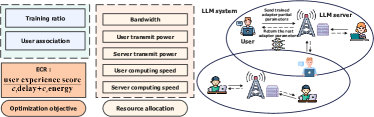
Figure 1: Optimizing the ECR of an LLM system with $N$ users and $M$ servers through joint optimization of user association, offloading, and resource allocation.

II-A System scenario

As presented in Fig. 1, the LLM-based mobile edge computing system contains multiple servers that distribute tailored LLM models or emulators to various mobile users. Given the computational constraints of some mobile users, a hybrid approach is adopted: users train the first few layers locally with their datasets while freezing the other layers. After training, users send these layer parameters of their adapters to the server. Once the server receives those layer parameters, it completes the training of the remaining layers while freezing the layers trained by the users. After training, the server sends the refined parameters back to the users. This collaborative mechanism ensures efficient and personalized LLM services, compensating for individual users’ computational limitations.

II-B System model

We consider a system comprising $N$ mobile users and $M$ LLM servers. We use $n$ and $m$ as indices for a VR user and a LLM server, respectively, where $n\in\mathcal{N}:=\{1,2,\cdots,N\}$ and $m\in\mathcal{M}:=\{1,2,\cdots,M\}$. Each user is connected to one and only one server; i.e., $\sum_{m\in\mathcal{M}}x_{n,m}=1$. We introduce indicator variables $x_{n,m}\in\{0,1\}$ to characterize the connection between users and servers; specifically, $x_{n,m}=1$ (resp, $0$) means that the $n$-th user is connected (resp., not connected) to the $m$-th server. For example, if $x_{n,m}=1$, it means that the $n$-th user only connects to the $m$-th server and $x_{n,m^{\prime}}=0$ for $m{{}^{\prime}}\in\mathcal{M}\setminus\{m\}$.

II-B1 Time consumption

We consider frequency-division multiple access (FDMA) so that communication among users and servers would not interfere. The transmission rate from user $n$ to the chosen edge server $m$ is $r_{n,m}(b_{n,m},p_{n})=b_{n,m}\log_{2}(1+\frac{g_{n,m}p_{n}}{\sigma^{2}b_{n,m}})$, where $\sigma^{2}$ is the noise power, $b_{n,m}$ is the allocated bandwidth between user $n$ and server $m$, $p_{n}$ is the transmit power of user $n$, $g_{n,m}$ is the channel gain and can be further expressed by $g_{n,m}=h_{n,m}l_{n,m}$, where $h_{n,m}$ is the large-scale slow-fading component capturing effects of path loss and shadowing and $l_{n,m}$ is the small-scale Rayleigh fading.

In Parameter-Efficient Fine-Tuning (PEFT) strategies for large language models, the concept is to introduce ”adapters” - smaller neural network components. These are placed within the model, enabling task-specific customization while largely keeping the pre-trained parameters unchanged. By doing this, there’s no need for the exhaustive retraining of the complete model. If we consider inserting an adapter between two layers with dimensions $d_{in}$ and $d_{out}$, the design usually involves: 1. A down-projection from $d_{in}$ to a reduced dimension $d_{adapt}$. 2. An up-projection from $d_{adapt}$ back to $d_{out}$. Accounting for weights and biases in these transformations, the total size of the adapter’s parameters, $d$, can be captured as: $d=d_{in}\times d_{adapt}+d_{adapt}\times d_{out}+d_{adapt}+d_{out}$. For any given user, represented by $n$, the parameter size of the adapter, $d_{n}$, can differ. This could be due to user-specific requirements or constraints. Hence, $d_{n}$ links the inherent complexity of the LLM, the architecture of the adapter, and the unique data requirements of user $n$.

User training and sending adapter parameter phases. Based on the above discussion, assume the total adapter parameter size at user $n$ is $d_{n}$. The adapter parameter size trained by user $n$ is $\varphi_{n}d_{n}$, $\varphi_{n}\in[0,1]$. User $n$ trains the first $\varphi_{n}d_{n}$ layer parameters with the local datasets. The training time consumed is $T^{(t_{1})}_{n,m}=\frac{t_{n}\varphi_{n}d_{n}e_{n}}{g_{n}F_{n}}$. $t_{n}$ is the FLOPs of all tokens for each adapter parameter of the user $n$. $e_{n}$ is the number of local training epochs. $g_{n}$ is the available GPU number of user $n$. $F_{n}$ is the available GPU computation speed of user $n$, defined as floating point operations (FLOPs). After local training and the user-server connection algorithm (this can be complicated by choosing the nearest neighbor server sets, then choosing the server with the lowest transmission time, and finally finishing all user-server connections), user $n$ transmits $\varphi_{n}d_{n}$ adapter parameters to the server $m$. The transmission time from the user $n$ to the server $m$ is $T^{(t_{2})}_{n,m}=\frac{x_{n,m}\varphi_{n}d_{n}\omega_{b}}{r_{n,m}}$, where $\omega_{b}$ is the bits number used to represent each parameter. For example, if we use the “float32” floating-point number, $\omega_{b}$ will be 32.

Server training and returning adapter parameter phases. After receiving the partial adapter parameters $\varphi_{n}d_{n}$ from the user $n$, the server $m$ trains the remaining part of the adapter with the shared user datasets and the training delay is $T^{(t_{3})}_{n,m}=\frac{t_{n}(1-\varphi_{n})x_{n,m}d_{n}e_{m}}{g_{m}F_{m}}$. $e_{m}$ is the number of server training epochs. $g_{m}$ is the available GPU number of server $m$. $F_{m}$ is the available GPU computation speed of server $m$. Then, Server $m$ transmits the results to the user $n$, and the delay is $T^{(t_{4})}_{n,m}=\frac{x_{n,m}(1-\varphi_{n})d_{n}\omega_{b}}{r_{m,n}}$, where $r_{m,n}=b_{n,m}\log_{2}(1+\frac{g_{n,m}p_{m}}{\sigma^{2}b_{n,m}})$. We assume the path loss and bandwidth between the downlink and uplink are the same. The time consumed on the server side is

$$\textstyle T_{s,n,m}=T^{(t_{2})}_{n,m}+T^{(t_{3})}_{n,m}.$$ (1)

The time consumed on the user side is

$$\textstyle T_{u,n,m}=T^{(t_{1})}_{n,m}+T^{(t_{4})}_{n}.$$ (2)

Therefore, the total delay will be

$$\textstyle T_{total} \textstyle=T_{s,n,m}+T_{u,n,m}$$

$$\textstyle=\frac{t_{n}\varphi_{n}d_{n}e_{n}}{g_{n}F_{n}}\!\!+\!\!\frac{x_{n,m}\varphi_{n}d_{n}\omega_{b}}{r_{n,m}}\!\!+\!\!\frac{t_{n}(1-\varphi_{n})x_{n,m}d_{n}e_{m}}{g_{m}F_{m}}$$

$$\textstyle+\frac{x_{n,m}(1-\varphi_{n})d_{n}\omega_{b}}{r_{m,n}}.$$ (3)

II-B2 Energy consumption

Based on the delay discussion, we then compute the energy consumption in this system. Energy used for user $n$ training the adapter locally can be calculated by $E^{(t_{1})}_{n,m}=e_{n}\kappa_{n}\varphi_{n}d_{n}t_{n}F^{2}_{n}$ [6]. $\kappa_{n}$ is the computational efficiency of user $n$’s GPUs, denoting the power growth rate corresponding to rising computing speeds. Energy used for transmitting data from the $n$-th user to the server $m$ is given as $E^{(t_{2})}_{n,m}=p_{n}T^{(t_{2})}_{n,m}=p_{n}\frac{x_{n,m}\varphi_{n}d_{n}\omega_{b}}{r_{n,m}}$. Energy for server training $\varphi_{n}d_{n}$ adapter parameters is given as $E^{(t_{3})}_{n,m}=e_{m}\kappa_{m}x_{n,m}(1-\varphi_{n})d_{n}t_{n}F_{m}^{2}$. $\kappa_{m}$ is the computational efficiency of server $m$’s GPUs. Energy caused by $m$-th server transmitting trained adapter parameters to user $n$ is $E^{(t_{4})}_{n,m}=p_{m}T^{(t_{4})}_{n,m}=p_{m}\frac{x_{n,m}(1-\varphi_{n})d_{n}\omega_{b}}{r_{m,n}}$. Thus, the total energy consumption can be formulated as follows:

$$\textstyle E_{total} \textstyle=\sum\limits_{n\in\mathcal{N},m\in\mathcal{M}}(E_{u,n,m}+E_{s,n,m})$$

$$\textstyle=\sum\limits_{n\in\mathcal{N},m\in\mathcal{M}}(E^{(t_{1})}_{n,m}+E^{(t_{2})}_{n,m}+E^{(t_{3})}_{n,m}+E^{(t_{4})}_{n,m})$$

$$\textstyle=\sum\limits_{n\in\mathcal{N},m\in\mathcal{M}}(p_{n}\frac{x_{n,m}\varphi_{n}d_{n}\omega_{b}}{r_{n,m}}+p_{m}\frac{x_{n,m}(1-\varphi_{n})d_{n}\omega_{b}}{r_{m,n}}$$

$$\textstyle+\!e_{n}\kappa_{n}\varphi_{n}d_{n}t_{n}F^{2}_{n}\!+\!e_{m}\kappa_{m}x_{n,m}(1\!\!-\!\!\varphi_{n})d_{n}t_{n}F_{m}^{2}).$$ (4)

II-B3 User service experience score

We denote the service experience score of user $n$ that is connected to server $m$ as:

$$\textstyle v_{n,m}=\varpi_{1}\ln[1+\varpi_{2}(\frac{p_{m}}{p_{max}^{(m)}}+\frac{F_{n,m}}{F_{max}^{(m)}}+\frac{b_{n,m}}{b_{max}})],$$ (5)

where $\varpi_{1}$ determines the range of function value, $\varpi_{2}$ is used for normalization of $(\frac{p_{m}}{p_{max}^{(m)}}+\frac{F_{n,m}}{F_{max}^{(m)}}+\frac{b_{n,m}}{b_{max}})$. This function is jointly concave of $p_{m}$, $F_{n,m}$, and $b_{n,m}$ [7]. This user service experience score function is effective and sensitive in all value ranges of $(\frac{p_{m}}{p_{max}^{(m)}}+\frac{F_{n,m}}{F_{max}^{(m)}}+\frac{b_{n,m}}{b_{max}})$, which can describe each user’s subjective experience of the communication and computing resources obtained from the server.

II-C Optimization Problem

User connection $\bm{x}=(x_{n,m})|_{n\in\mathcal{N},m\in\mathcal{M}}$, $\bm{\varphi}=(\varphi_{n})|_{n\in\mathcal{N}}$, bandwidth $\bm{b}=(b_{n,m})|_{n\in\mathcal{N},m\in\mathcal{M}}$, transmission power $\bm{p_{u}}=(p_{n})|_{n\in\mathcal{N}}$ and $\bm{p_{s}}=(p_{m})|_{m\in\mathcal{M}}$, and GPU computation speed $\bm{f_{u}}=(F_{n})|_{n\in\mathcal{N}}$ and $\bm{f_{s}}=(F_{m})|_{m\in\mathcal{M}}$. Our goal is to maximize the user service experience-cost ratio (ECR):

$$\textstyle\frac{\mathcal{V}}{\omega_{t}T_{total}+\omega_{e}E_{total}}=$$

$$\textstyle\frac{\sum\limits_{n\in\mathcal{N},m\in\mathcal{M}}x_{n,m}v_{n,m}}{\omega_{t}(T_{s,n,m}+T_{u,n,m})+\omega_{e}(\sum\limits_{n\in\mathcal{N},m\in\mathcal{M}}(E^{(t_{1})}_{n,m}+E^{(t_{2})}_{n,m}+E^{(t_{3})}_{n,m}+E^{(t_{4})}_{n,m}))},$$ (6)

where $\omega_{t}$ and $\omega_{e}$ represent the weight values of delay and energy, respectively. In order to linearize the “maximize” term of $T_{total}$, we add an auxiliary variable $T$, which is constrained to be greater than or equal to $T_{total}$. Besides, we utilize Dinkelbach’s Algorithm [8] by adding an additional variable $y$, which is obtained from the ECR value in the previous iteration. Then, the fractional programming in the trust-cost ratio is transformed into the following problem:

$$\max\limits_{\bm{x},\bm{\varphi},\bm{b},\bm{p_{u}},\bm{p_{s}},\bm{f_{u}},\bm{f_{s}},T}$$

$$\big{\{}\!\!\!\!\sum\limits_{n\in\mathcal{N},m\in\mathcal{M}}\!\!\!\![x_{n,m}v_{n,m}-y\omega_{e}(E_{u,n,m}\!\!+\!\!E_{s,n,m})]\big{\}}-y\omega_{t}T$$ (7)

s.t. $$x_{n,m}\in\{0,1\},\forall n,m$$ (7a)

$$\sum\limits_{m\in\mathcal{M}}x_{n,m}=1,\forall n$$ (7b)

$$\varphi_{n}\in[0,1],\forall n$$ (7c)

$$\sum\limits_{n\in\mathcal{N}}x_{n,m}b_{n,m}\leq b_{max},\forall m$$ (7d)

$$p_{n}\leq p^{(n)}_{max},\forall n$$ (7e)

$$\sum\limits_{n\in\mathcal{N}}x_{n,m}p_{n,m}\leq p^{(m)}_{max},\forall m$$ (7f)

$$F_{n}\leq F^{(n)}_{max},\forall n$$ (7g)

$$\sum\limits_{n\in\mathcal{N}}x_{n,m}F_{m}\leq F^{(m)}_{max},\forall m$$ (7h)

$$b_{n,m}\!\geq\!0,p_{n}\!\geq\!0,p_{n,m}\!\geq\!0,F_{n}\!\geq\!0,F_{m}\!\geq\!0,\forall n,m$$ (7i)

$$T_{s,n,m}+T_{u,n,m}\leq T,\forall n,m$$ (7j)

Based on Dinkelbach’s Algorithm, we iteratively optimize $y$ and problem (7). Specifically, at the $i$-th iteration, given $y^{(i-1)}$, we first obtain $\bm{x}^{(i)},\bm{\varphi}^{(i)},\bm{b}^{(i)},\bm{p_{u}}^{(i)},\bm{p_{s}}^{(i)},\bm{f_{u}}^{(i)},\bm{f_{s}}^{(i)},T^{(i)}$ by solving the optimization problem 7; then we calculate $y^{(i)}$ with the given $\bm{x}^{(i)},\bm{\varphi}^{(i)},\bm{b}^{(i)},\bm{p_{u}}^{(i)},\bm{p_{s}}^{(i)},\bm{f_{u}}^{(i)},\bm{f_{s}}^{(i)},T^{(i)}$. Repeat the above operations until the solutions converge. In the following section, we consider using the alternating optimization method (AO) to tackle the complex problem (7).

Roadmap of the whole algorithm. First, we decompose the outer fractional structure of the original ECR problem using Dinkelbach algorithm and sequentially optimize $\bm{x},\bm{\varphi}$ and $\bm{b},\bm{p_{u}},\bm{p_{s}},\bm{f_{u}},\bm{f_{s}}$ using the AO method. In the first step of AO, we fix $\bm{b},\bm{p_{u}},\bm{p_{s}},\bm{f_{u}},\bm{f_{s}}$ and optimize $\bm{x},\bm{\varphi},T$. We transform the optimization problem in the first step of AO into a Quadratically Constrained Quadratic Program (QCQP) and solve it using Semidefinite Relaxation (SDR) and the Hungarian algorithm. In the second step of AO, we fix $\bm{x},\bm{\varphi}$ and optimize $\bm{b},\bm{p_{u}},\bm{p_{s}},\bm{f_{u}},\bm{f_{s}},T$. During the optimization in the second step of AO, we propose a new fractional programming method to transform this non-convex problem into a convex one. Finally, we calculate $y$ based on the obtained solutions and repeat the aforementioned process until $y$ converges. In this algorithm, since we utilize Dinkelbach’s algorithm, alternating optimization, semidefinite relaxation, Hungarian algorithm, and fractional programming, we refer to this algorithm as the DASHF Algorithm.

III Our proposed DASHF Algorithm to solve the optimization problem

Assuming that $y$ is given, we need to optimize $\bm{x},\bm{\varphi},\bm{b},\bm{p_{u}},\bm{p_{s}},\bm{f_{u}},\bm{f_{s}},T$. In the outermost loops, we iteratively optimize $y$; In the innermost loops, we iteratively optimize $\bm{x},\bm{\varphi},\bm{b},\bm{p_{u}},\bm{p_{s}},\bm{f_{u}},\bm{f_{s}},T$. However, it is still difficult to optimize them in parallel. Thus, we consider operating two inner AO steps to solve it. At the $i$-th iteration,

1. Optimize $\bm{x}$, $\bm{\varphi}$, $T$, given $\bm{b}$, $\bm{p_{u}}$, $\bm{p_{s}}$, $\bm{f_{u}}$, $\bm{f_{s}}$. Assuming that $\bm{b}^{(i-1)}$, $\bm{p_{u}}^{(i-1)},$$\bm{p_{s}}^{(i-1)}$, $\bm{f_{u}}^{(i-1)}$, $\bm{f_{s}}^{(i-1)}$, $y^{(i-1)}$ are given, we optimize $\bm{x}^{(i)}$, $\bm{\varphi}^{(i)}$, $T^{(i)}$.

2. Optimize $\bm{b}$,$\bm{p_{u}}$,$\bm{p_{s}}$,$\bm{f_{u}}$,$\bm{f_{s}}$,$T$, given $\bm{x}$, $\bm{\varphi}$. Assuming that $\bm{x}^{(i-1)}$, $\bm{\varphi}^{(i-1)}$,$y^{(i-1)}$ are given, we optimize $\bm{b}^{(i)}$,$\bm{p_{u}}^{(i)}$,$\bm{p_{s}}^{(i)}$,$\bm{f_{u}}^{(i)}$,$\bm{f_{s}}^{(i)}$,$T^{(i)}$.

III-A AO Part 1: Optimizing $\bm{x},\bm{\varphi},T$, given $\bm{b},\bm{p_{u}},\bm{p_{s}},\bm{f_{u}},\bm{f_{s}}$

Given $\bm{b},\bm{p_{u}},\bm{p_{s}},\bm{f_{u}},\bm{f_{s}},T$, we optimize $\bm{x},\bm{\varphi},T$. The optimization problem will be:

$$\!\!\!\max\limits_{\bm{x},\bm{\varphi},T}\!\!\!\! \sum\limits_{n\in\mathcal{N},m\in\mathcal{M}}\!\!\!\!\!\![x_{n,m}v_{n,m}\!-\!y\omega_{e}(E_{u,n,m}\!+\!E_{s,n,m})]-y\omega_{t}T$$ (8)

s.t. $$(\text{\ref{x_constr1}}),(\text{\ref{x_constr2}}),(\text{\ref{varphi_constr}}),(\text{\ref{x_b_constr}}),(\text{\ref{x_ps_constr}}),(\text{\ref{x_fs_constr}}),(\text{\ref{T_constr}}).$$

$x_{n,m}$ are binary variables and this is a mixed-integer nonlinear programming problem. We rewrite $x_{n,m}\in\{0,1\},\forall n,m$ as $x_{n,m}(x_{n,m}-1)=0,\forall n,m$. The optimization problem will be rewritten as:

$$\!\!\!\!\max\limits_{\bm{x},\bm{\varphi},T}\!\!\!\!\!\sum\limits_{n\in\mathcal{N},m\in\mathcal{M}}\!\!\!\!\!\!\!\![x_{n,m}v_{n,m}\!-\!y\omega_{e}(E_{u,n,m}\!+\!E_{s,n,m})]-y\omega_{t}T$$ (9)

$$\text{s.t.}\quad x_{n,m}(x_{n,m}-1)=0,\forall n,m$$ (9a)

$$\quad\quad(\text{\ref{x_constr2}}),(\text{\ref{varphi_constr}}),(\text{\ref{x_b_constr}}),(\text{\ref{x_ps_constr}}),(\text{\ref{x_fs_constr}}),(\text{\ref{T_constr}}).$$

We substitute the expression of $E_{u,n,m}+E_{s,n,m}$ into problem (9) and convert the $\max$ problem in problem (9) to a $\min$ problem (10).

$$\min\limits_{\bm{x},\bm{\varphi},T}y\omega_{t}T\!\!+\!\!\!\!\!\!\!\!\sum\limits_{n\in\mathcal{N},m\in\mathcal{M}}\!\!\!\!\!\!\!\!\{y\omega_{e}(\frac{p_{n}d_{n}\omega_{b}}{r_{n,m}}\!\!-\!\!\frac{p_{m}d_{n}\omega_{b}}{r_{m,n}}\!\!-\!e_{m}\kappa_{m}d_{n}t_{n}F_{m}^{2})$$

$$x_{n,m}\varphi_{n}+[y\omega_{e}(\frac{p_{m}d_{n}\omega_{b}}{r_{m,n}}+e_{m}\kappa_{m}d_{n}t_{n}F_{m}^{2})-v_{n,m}]x_{n,m}$$

$$\quad+y\omega_{e}(e_{n}\kappa_{n}d_{n}t_{n}F_{n}^{2})\varphi_{n}\}$$ (10)

$$\text{s.t.}\quad\quad(\text{\ref{x_constr1_new}}),(\text{\ref{x_constr2}}),(\text{\ref{varphi_constr}}),(\text{\ref{x_b_constr}}),(\text{\ref{x_ps_constr}}),(\text{\ref{x_fs_constr}}),(\text{\ref{T_constr}}).$$

Let $G_{n,m}\!=\!y\omega_{e}(\frac{p_{n}d_{n}\omega_{b}}{r_{n,m}}-\frac{p_{m}d_{n}\omega_{b}}{r_{m,n}}-e_{m}\kappa_{m}d_{n}t_{n}F_{m}^{2})$, $A_{n,m}=y\omega_{e}(e_{n}\kappa_{n}d_{n}t_{n}F_{n}^{2})$, and $B_{n,m}=y\omega_{e}(\frac{p_{m}d_{n}\omega_{b}}{r_{m,n}}+e_{m}\kappa_{m}d_{n}t_{n}F_{m}^{2})-v_{n,m}$. Let $\mathbf{A}=[A_{n}]|_{n\in\mathcal{N}}$, $\mathbf{B}=[B_{n,m}]|_{n\in\mathcal{N},m\in\mathcal{M}}$, and $\mathbf{G}=[G_{n,m}]|_{n\in\mathcal{N},m\in\mathcal{M}}$. The optimization problem (10) can be rewritten as

$$\mathcal{P}_{1}: \min\limits_{\bm{x},\bm{\varphi},T}y\omega_{t}T\!\!+\!\!\sum\limits_{n\in\mathcal{N}}A_{n}\varphi_{n}+\!\!\!\!\!\sum\limits_{n\in\mathcal{N},m\in\mathcal{M}}\!\!\!\!\!(B_{n,m}x_{n,m}+$$

$$\quad\quad\quad\quad G_{n,m}x_{n,m}\varphi_{n})$$ (11)

$$\text{s.t.}\quad(\text{\ref{x_constr1_new}}),(\text{\ref{x_constr2}}),(\text{\ref{varphi_constr}}),(\text{\ref{x_b_constr}}),(\text{\ref{x_ps_constr}}),(\text{\ref{x_fs_constr}}),(\text{\ref{T_constr}}).$$

This is a quadratically constrained quadratic program (QCQP) problem. Then, we need to get the standard form of the QCQP problem. Let $\bm{Q}=(\bm{\varphi}^{\intercal},\bm{x_{1}}^{\intercal},\cdots,\bm{x_{M}}^{\intercal})^{\intercal}$, where $\bm{\varphi}=(\varphi_{1},\cdots,\varphi_{N})^{\intercal}$ and $\bm{x_{m}}=(x_{1,m},\cdots,x_{n,m})^{\intercal},\forall m\in\mathcal{M}$. Let $\bm{e}_{i}$ denotes $(0,\cdots,\underset{\underset{i\text{-th}}{\uparrow}}{1},\cdots,0)^{\intercal}_{NM+N\times 1}$. Let $\bm{e}_{i,j}$ denotes $(\bm{e}_{i},\cdots,\bm{e}_{j})^{\intercal},i<j$. Then, $\sum\limits_{n\in\mathcal{N},m\in\mathcal{M}}G_{n,m}x_{n,m}\varphi_{n}$ can be expressed as $\bm{Q}^{\intercal}\text{diag}(\bm{G},\bm{0}_{NM\times 1})(\bm{e}_{N+1,NM+N},\bm{0}_{NM\times NM+N})^{\intercal}\bm{Q}$.Let

$$\mathbf{P}_{0}=\text{diag}(\bm{G},\bm{0}_{NM\times 1})(\bm{e}_{N+1,NM+N},\bm{0}_{NM\times NM+N})^{\intercal}.$$ (12)

$\sum\limits_{n\in\mathcal{N},m\in\mathcal{M}}B_{n,m}x_{n,m}$ can be expressed as $\mathbf{W}_{0}^{\intercal}\bm{Q}$, where $\mathbf{W}_{0}^{\intercal}=(\bm{B}_{1}^{\intercal},\cdots,\bm{B}_{M}^{\intercal})\bm{e}_{N+1,NM+N}$ and $\bm{B}_{i}^{\intercal}=(B_{1,i},\cdots,B_{N,i}),\forall i\in\mathcal{M}$. $\sum_{n\in\mathcal{N}}A_{n}\varphi_{n}$ can be expressed as $\mathbf{W}_{1}^{\intercal}\bm{Q}$, where $\mathbf{W}_{1}^{\intercal}=(A_{1},\cdots,A_{N})\bm{e}_{1,N}$. Let $P^{(\text{T1})}_{n,m}=-\frac{d_{n}\omega_{b}}{r_{m,n}}+\frac{d_{n}\omega_{b}}{r_{n,m}}-\frac{t_{n}d_{n}e_{m}}{g_{m}F_{m}}$, $P^{(\text{T2})}_{n}=\frac{t_{n}d_{n}e_{n}}{g_{n}F_{n}}$, and $P^{(\text{T3})}_{n,m}=\frac{t_{n}d_{n}e_{m}}{g_{m}F_{m}}+\frac{d_{n}\omega_{b}}{r_{m,n}}$. Let $\mathbf{P^{(\text{T1})}}=[P^{(\text{T1})}]|_{n\in\mathcal{N},m\in\mathcal{M}}$, $\mathbf{P^{(\text{T2})}}=[P^{(\text{T2})}]|_{n\in\mathcal{N}}$, $\mathbf{P^{(\text{T3})}}=[P^{(\text{T3})}]|_{n\in\mathcal{N},m\in\mathcal{M}}$. Let $\mathbf{P^{(\text{T4})}}=\text{diag}(\bm{P^{(\text{T1})}},\bm{0}_{NM\times 1})(\bm{e}_{N+1,NM+N},\bm{0}_{NM\times NM+N})^{\intercal}$, $\mathbf{P^{(\text{T5})}}_{1}^{\intercal}=(P^{(\text{T2})}_{1},\cdots,P^{(\text{T2})}_{N})\bm{e}_{1,N}$, ${\mathbf{P^{(\text{T6})}}}^{\intercal}=({\bm{P^{(\text{T3})}}_{1}}^{\intercal},\cdots,{\bm{P^{(\text{T3})}}_{M}}^{\intercal})\bm{e}_{N+1,NM+N}$, where ${\bm{P^{(\text{T3})}}_{i}}^{\intercal}=(P^{(\text{T3})}_{1,i},\cdots,P^{(\text{T3})}_{N,i}),\forall i\in\mathcal{M}$. Therefore, the optimization problem can be expressed as

$$\mathcal{P}_{2}: \min\limits_{\bm{Q},T}\quad\bm{Q}^{\intercal}\mathbf{P}_{0}\bm{Q}+\mathbf{W}_{0}^{\intercal}\bm{Q}+\mathbf{W}_{1}^{\intercal}\bm{Q}+y\omega_{t}T$$ (13)

s.t. $$\text{diag}(\bm{e}_{N+1,NM+N}^{\intercal}\bm{Q})(\text{diag}(\bm{e}_{N+1,NM+N}^{\intercal}\bm{Q})-\mathbf{I})=\mathbf{0}$$ (13a)

$$\text{diag}(\bm{e}_{\overline{1},\overline{M}}^{\intercal}\bm{e}_{N+1,NM+N}^{\intercal}\bm{Q})=\mathbf{I}$$ (13b)

$$\text{diag}(\bm{e}_{1,N}^{\intercal}\bm{Q})\leq\mathbf{I}$$ (13c)

$$\text{diag}(\bm{e}_{1,N}^{\intercal}\bm{Q})\geq\mathbf{0}$$ (13d)

$$\bm{B}^{\intercal}\bm{e}_{N+1,NM+N}^{\intercal}\bm{Q}-B_{max}\leq 0$$ (13e)

$$\bm{P}^{\intercal}\bm{e}_{N+1,NM+N}^{\intercal}\bm{Q}-P_{max}^{(m)}\leq 0$$ (13f)

$$\bm{F}^{\intercal}\bm{e}_{N+1,NM+N}^{\intercal}\bm{Q}-F_{max}^{(m)}\leq 0$$ (13g)

$$\bm{Q}^{\intercal}\mathbf{P}^{(\text{T4})}\bm{Q}+{\mathbf{P}^{(\text{T5})}}^{\intercal}\bm{Q}+{\mathbf{P}^{(\text{T6})}}^{\intercal}\bm{Q}\leq T,$$ (13h)

where $\bm{e}_{\overline{i},\overline{j}}$ denotes $(\bm{e}_{\overline{i}},\cdots,\bm{e}_{\overline{j}})^{\intercal},i<j$, $\bm{B}=(b_{1,1},\cdots,b_{n,m})^{\intercal}$, $\bm{P}=(P_{1,1},\cdots,p_{n,m})^{\intercal}$, and $\bm{F}=(F_{1,1},\cdots,F_{n,m})^{\intercal}$. The constraints $(\text{\ref{x_constr1_new}})$, $(\text{\ref{x_constr2}})$, $(\text{\ref{varphi_constr}})$, $(\text{\ref{x_b_constr}})$, $(\text{\ref{x_ps_constr}})$, $(\text{\ref{x_fs_constr}})$, $(\text{\ref{T_constr}})$ in $\mathcal{P}_{1}$ are transformed into the constraints $(\text{\ref{x_constr1_qcqp}})$, $(\text{\ref{x_constr2_qcqp}})$, $\{(\text{\ref{varphi_constr1_qcqp}})$, $(\text{\ref{varphi_constr2_qcqp}})\}$, $(\text{\ref{x_b_constr_qcqp}})$, $(\text{\ref{x_ps_constr_qcqp}})$, $(\text{\ref{x_fs_constr_qcqp}})$, $(\text{\ref{T_constr_qcqp}})$ in $\mathcal{P}_{2}$, respectively. Problem (13) is the standard QCQP form. However, it is still non-convex. Then, we need to utilize the semidefinite programming (SDP) method to transform this QCQP problem into a semidefinite relaxation (SDR) problem. Let $\mathbf{S}=(\bm{Q}^{\intercal},1)^{\intercal}(\bm{Q}^{\intercal},1)$. Let $\bm{e}_{i\rightarrow j}$ denotes $(0,\cdots,\underset{\underset{i\text{-th}}{\uparrow}}{1},1,\cdots,\underset{\underset{j\text{-th}}{\uparrow}}{1},0,\cdots,0)^{\intercal},i<j$. Then we obtain the SDR problem

$$\mathcal{P}_{3}:\min\limits_{\bm{S},T}\quad \text{Tr}(\mathbf{P}_{1}\mathbf{S})$$ (14)

s.t. $$\text{Tr}(\mathbf{P}_{2}\mathbf{S})=0$$ (14a)

$$\text{Tr}(\mathbf{P}_{3}\mathbf{S})=0$$ (14b)

$$\text{Tr}(\mathbf{P}_{4}\mathbf{S})\leq 0$$ (14c)

$$\text{Tr}(\mathbf{P}_{5}\mathbf{S})\leq 0$$ (14d)

$$\text{Tr}(\mathbf{P}_{6}\mathbf{S})\leq 0$$ (14e)

$$\text{Tr}(\mathbf{P}_{7}\mathbf{S})\leq 0$$ (14f)

$$\text{Tr}(\mathbf{P}_{8}\mathbf{S})\leq T$$ (14g)

$$\mathbf{S}\succeq 0,$$ (14h)

where

$$\mathbf{P}_{1}=\left(\begin{array}[]{cc}\mathbf{P}_{0}&\frac{1}{2}(\mathbf{W}_{0}+\mathbf{W}_{1})\\ \frac{1}{2}(\mathbf{W}_{0}+\mathbf{W}_{1})^{\intercal}&y\omega_{t}T\end{array}\right),$$

$$\mathbf{P}_{2}=\left(\begin{array}[]{cc}\bm{e}_{i}^{\intercal}\bm{e}_{i}&-\frac{1}{2}\bm{e}_{i}\\ -\frac{1}{2}\bm{e}_{i}^{\intercal}&0\end{array}\right),\forall i\in\{1,\cdots,NM\}$$

$$\mathbf{P}_{3}=\left(\begin{array}[]{cc}\mathbf{0}_{NM+N\times NM+N}&\frac{1}{2}(\bm{e}_{\overline{i}}\bm{e}_{N+1,NM+N}^{\intercal})\\ \frac{1}{2}(\bm{e}_{\overline{i}}\bm{e}_{N+1,NM+N}^{\intercal})^{\intercal}&-1\end{array}\right),$$ (17)

$$\forall i\in\{1,\cdots,N\}$$

$$\mathbf{P}_{4}=\left(\begin{array}[]{cc}\mathbf{0}_{NM+N\times NM+N}&\frac{1}{2}\bm{e}_{i}\\ \frac{1}{2}\bm{e}_{i}^{\intercal}&-1\end{array}\right),\forall i\in\{1,\cdots,N\}$$

$$\mathbf{P}_{5}=\left(\begin{array}[]{cc}\mathbf{0}_{NM+N\times NM+N}&\frac{1}{2}\bm{B}\bm{e}_{N+1,NM+N}\\ \frac{1}{2}(\bm{B}\bm{e}_{N+1,NM+N})^{\intercal}&-B_{max}\end{array}\right),$$

$$\mathbf{P}_{6}=\left(\begin{array}[]{cc}\mathbf{0}_{NM+N\times NM+N}&\frac{1}{2}\bm{P}\bm{e}_{N+1,NM+N}\\ \frac{1}{2}(\bm{P}\bm{e}_{N+1,NM+N})^{\intercal}&-P_{max}^{(m)}\end{array}\right),$$

$$\mathbf{P}_{7}=\left(\begin{array}[]{cc}\mathbf{0}_{NM+N\times NM+N}&\frac{1}{2}\bm{F}\bm{e}_{N+1,NM+N}\\ \frac{1}{2}(\bm{F}\bm{e}_{N+1,NM+N})^{\intercal}&-F_{max}^{(m)}\end{array}\right),$$

$$\mathbf{P}_{8}=\left(\begin{array}[]{cc}\mathbf{P}^{(\text{T4})}&\frac{1}{2}(\mathbf{P}^{(\text{T5})}+\mathbf{P}^{(\text{T6})})\\ \frac{1}{2}(\mathbf{P}^{(\text{T5})}+\mathbf{P}^{(\text{T6})})^{\intercal}&0\end{array}\right).$$

The constraints $(\text{\ref{x_constr1_qcqp}})$, $(\text{\ref{x_constr2_qcqp}})$, $(\text{\ref{varphi_constr1_qcqp}})$, $(\text{\ref{varphi_constr2_qcqp}})$, $(\text{\ref{x_b_constr_qcqp}})$, $(\text{\ref{x_ps_constr_qcqp}})$, $(\text{\ref{x_fs_constr_qcqp}})$, $(\text{\ref{T_constr_qcqp}})$ in $\mathcal{P}_{2}$ are transformed into the constraints $(\text{\ref{x_constr1_sdr}}),(\text{\ref{x_constr2_sdr}}),(\text{\ref{varphi_constr_sdr}}),(\text{\ref{S_constr_sdr}}),(\text{\ref{x_b_constr_sdr}}),(\text{\ref{x_ps_constr_sdr}}),(\text{\ref{x_fs_constr_sdr}}),(\text{\ref{T_constr_sdr}})$ in $\mathcal{P}_{3}$, respectively. Drop the constraint $\text{rank}(\mathbf{S})=1$ and the objective function and the constraints are all convex. Then this SDR problem will be solved in polynomial time by common convex solvers. By solving this SDR problem, we can get a continuous solution of $\bm{Q}$. However, this solution is the lower bound of the optimal solution and it may not guarantee the constraint $\text{rank}(\mathbf{S})=1$. Therefore, we need to use rounding techniques to recover the solution. The latter $NM$ elements in $\bm{Q}$ is $x_{n,m}$, for all $n\in\mathcal{N},m\in\mathcal{M}$, which means that user $n$ is fractional connected to server $m$. Then, find all user $n$ that $\sum\limits_{m\in\mathcal{M}}x_{n,m}>1$. For these users, modify $x_{n,m}$ as $\frac{x_{n,m}}{|\sum\limits_{m\in\mathcal{M}}x_{n,m}|}$. Use the Hungarian algorithm [9] with augmented zero vectors to find the best matching with the maximum weight and denote this matching as a set $\mathcal{X}_{matching}$. For nodes $n$ and $m$ in $\mathcal{X}_{matching}$, let $x_{n,m}=1$, else $x_{n,m}=0$, and denote this integer association result as $\bm{x}_{\sharp}$. Then substitute $\bm{x}_{\sharp}$ into Problem (13) to obtain the optimal $\bm{\varphi}$.

III-B AO Part 2: Optimizing $\bm{b},\bm{p_{u}},\bm{p_{s}},\bm{f_{u}},\bm{f_{s}},T$, given $\bm{x},\bm{\varphi}$

Given $\bm{x}$ and $\bm{\varphi}$, the remaining optimization problem is shown as (18).

$$\max\limits_{\bm{b},\bm{p_{u}},\bm{p_{s}},\bm{f_{u}},\bm{f_{s}},T}\quad\sum\limits_{n\in\mathcal{N},m\in\mathcal{M}}x_{n,m}v_{n,m}-y\bigg{\{}\omega_{t}T$$

$$+\omega_{e}\big{\{}\sum\limits_{n\in\mathcal{N}}e_{n}\kappa_{n}\varphi_{n}d_{n}t_{n}F^{2}_{n}+\sum\limits_{n\in\mathcal{N},m\in\mathcal{M}}\{p_{n}\frac{x_{n,m}\varphi_{n}d_{n}\omega_{b}}{r_{n,m}}$$

$$+\!e_{m}\kappa_{m}x_{n,m}(1\!\!-\!\!\varphi_{n})d_{n}t_{n}F_{n,m}^{2}\!\!+\!p_{m}\frac{x_{n,m}(1\!\!-\!\!\varphi_{n})d_{n}\omega_{b}}{r_{m,n}}\}\big{\}}\bigg{\}}$$ (18)

$$\text{s.t.}\quad(\text{\ref{x_b_constr}}),(\text{\ref{pu_constr}}),(\text{\ref{x_ps_constr}}),(\text{\ref{fu_constr}}),(\text{\ref{x_fs_constr}}),(\text{\ref{nonnegative_constr}}),(\text{\ref{T_constr}}).$$

We first Let

$$\textstyle\mathcal{F}(\bm{b},\bm{p_{s}},\bm{f_{u}},\bm{f_{s}},T)=\!\!\!\!\sum\limits_{n\in\mathcal{N},m\in\mathcal{M}}\!\!x_{n,m}v_{n,m}-y\omega_{t}T$$

$$\textstyle-y\omega_{e}\big{\{}\sum\limits_{n\in\mathcal{N}}e_{n}\kappa_{n}\varphi_{n}d_{n}t_{n}F^{2}_{n}$$

$$\textstyle+\sum\limits_{n\in\mathcal{N},m\in\mathcal{M}}\!\!\!\!\!e_{m}\kappa_{m}x_{n,m}(1-\varphi_{n})d_{n}t_{n}F_{n,m}^{2}\big{\}}.$$ (19)

It’s easy to justify that $\mathcal{F}(\bm{b},\bm{p_{s}},\bm{f_{u}},\bm{f_{s}},T)$ is concave. Then, the optimization objective function is

$$\textstyle\mathcal{F}(\bm{b},\bm{p_{s}},\bm{f_{u}},\bm{f_{s}},T)\!-\!y\omega_{e}\!\!\!\!\!\!\sum\limits_{n\in\mathcal{N},m\in\mathcal{M}}\!\!\!\!\!\!\!(\frac{p_{n}x_{n,m}\varphi_{n}d_{n}\omega_{b}}{r_{n,m}}\!$$

$$\textstyle+\!\frac{p_{m}x_{n,m}(1-\varphi_{n})d_{n}\omega_{b}}{r_{m,n}}),$$ (20)

where $\frac{p_{n}x_{n,m}\varphi_{n}d_{n}\omega_{b}}{r_{n,m}}+\frac{p_{m}x_{n,m}\varphi_{n}d_{n}\omega_{b}}{r_{m,n}}$ is non-convex or concave. Then, according to the fractional programming technique introduced in the Section IV in [1], we let $z_{1,n,m}=\frac{1}{2p_{n}x_{n,m}\varphi_{n}d_{n}\omega_{b}r_{n,m}}$ and $z_{2,n,m}=\frac{1}{2p_{m}x_{n,m}\varphi_{n}d_{n}\omega_{b}r_{m,n}}$. The optimization objective function can be expressed as

$$\textstyle\mathcal{F}(\bm{b},\bm{p_{s}},\bm{f_{u}},\bm{f_{s}},T)$$

$$\textstyle-y\omega_{e}\sum\limits_{n\in\mathcal{N},m\in\mathcal{M}}[(p_{n}x_{n,m}\varphi_{n}d_{n})^{2}z_{1,n,m}+$$

$$\textstyle\frac{1}{4(b_{n,m}\log_{2}(1+\frac{g_{n,m}p_{n}}{\sigma^{2}b_{n,m}}))^{2}z_{1,n,m}}\!\!+\!\!(p_{m}x_{n,m}\varphi_{n}d_{n}\omega_{p})^{2}z_{2,n,m}$$

$$\textstyle+\frac{1}{4(b_{m,n}\log_{2}(1+\frac{g_{m,n}p_{m}}{\sigma^{2}b_{m,n}}))^{2}z_{2,n,m}}].$$ (21)

The complete transformation optimization problem is shown as (22).

$$\max\limits_{\bm{b},\bm{p_{u}},\bm{p_{s}},\bm{f_{u}},\bm{f_{s}},T}\mathcal{F}(\bm{b},\bm{p_{s}},\bm{f_{u}},\bm{f_{s}},T)$$

$$\quad\quad\quad\quad\quad-y\omega_{e}\sum\limits_{n\in\mathcal{N},m\in\mathcal{M}}[(p_{n}x_{n,m}\varphi_{n}d_{n})^{2}z_{1,n,m}$$

$$\quad\quad\quad\quad\quad+\frac{1}{4(b_{n,m}\log_{2}(1+\frac{g_{n,m}p_{n}}{\sigma^{2}b_{n,m}}))^{2}z_{1,n,m}}$$

$$\quad\quad\quad\quad\quad+(p_{m}x_{n,m}\varphi_{n}d_{n}\omega_{p})^{2}z_{2,n,m}$$

$$\quad\quad\quad\quad\quad+\frac{1}{4(b_{m,n}\log_{2}(1+\frac{g_{m,n}p_{m}}{\sigma^{2}b_{m,n}}))^{2}z_{2,n,m}}]$$ (22)

$$\quad\text{s.t.}(\text{\ref{x_b_constr}}),(\text{\ref{pu_constr}}),(\text{\ref{x_ps_constr}}),(\text{\ref{fu_constr}}),(\text{\ref{x_fs_constr}}),(\text{\ref{nonnegative_constr}}),(\text{\ref{T_constr}}).$$

If $\bm{z}_{1}=(z_{1,1,1},\cdots,z_{1,n,m})^{\intercal}$ and $\bm{z}_{2}=(z_{2,1,1},\cdots,z_{2,n,m})^{\intercal}$ is given, the objective function (22) is concave. At the $i$-th iteration, $[y^{(i)}$, $\bm{z}_{1}^{(i)}$, $\bm{z}_{2}^{(i)}]$ are first calculated with the solution $[\bm{b}^{(i-1)},\bm{p_{u}}^{(i-1)},\bm{p_{s}}^{(i-1)},\bm{f_{u}}^{(i-1)},\bm{f_{s}}^{(i-1)}]$. Then, $[\bm{b}^{(i)},\bm{p_{u}}^{(i)},\bm{p_{s}}^{(i)},\bm{f_{u}}^{(i)},\bm{f_{s}}^{(i)}]$ can be obtained by solving the concave problem (22) with $[y^{(i)},\bm{z}_{1}^{(i)},\bm{z}_{2}^{(i)}]$. Thus, the optimization problem is concave and can be solved by common convex solvers. More detailed proofs can be seen in [1].

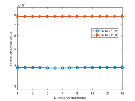
(a) Convergence of Algorithm AO-Part 1

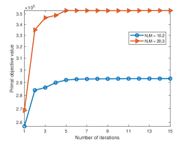
(b) Convergence of Algorithm AO-Part 2

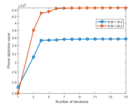
(c) Convergence of Algorithm DASHF

Figure 2: Convergence of the proposed Algorithms

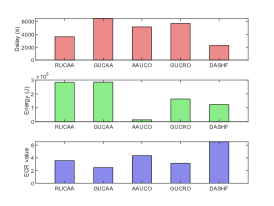
(a) Resource consumption and ECR of baselines and proposed DASHF Algorithm

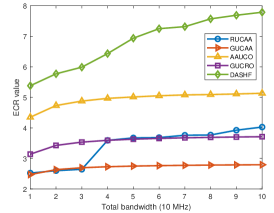
(b) ECR under different total bandwidth

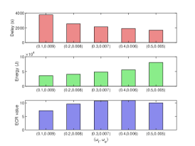
(c) Resources consumption and ECR under different $(\omega_{t},\omega_{e})$

Figure 3: ECR comparisons under different cases

IV Simulation Results

In this section, we first introduce the default settings for the numerical simulations. Subsequently, we verify the convergence of the proposed DASHF algorithm and compare it with other baselines to validate its effectiveness. Then, we adjust the available communication and computational resources as well as the cost weight parameters to analyze their impacts on the ECR.

IV-A Default settings

We consider a network topology of 1000 m $\times$ 1000 m with 10 mobile users and 2 servers. The large-scale fading $h_{n,m}$ between the user $n$ and server $m$ is modeled as $128.1+37.6\log_{10}d_{n,m}$, where $d_{n,m}$ denotes the Euclidean distance between the user $n$ and server $m$. The small-scale fading is the Rayleigh fading. Gaussian noise power $\sigma^{2}$ is $-134$dBm. The total bandwidth for each server $b_{max}$ is 10 MHz. The maximum transmit power of mobile users $p_{max}^{(n)}$ is 0.2 W. The maximum transmit power of servers $p_{max}^{(m)}$ is 10 W. We assume the GPU resource utilization is $0.55$ for users and servers. The maximum GPU computation speed of mobile users $F_{max}^{(n)}$ is $19.58$ TFLOPs with four GTX 1080 GPUs and that of servers $F_{max}^{(m)}$ is $1372.8$ TFLOPs with eight A100 GPUs. The effective switched capacitance of mobile users and servers ($\kappa_{n}$ and $\kappa_{m}$) is $10^{-38}$. We refer to the adapter parameter sizes in [3] and [2]. The adapter parameter sizes of mobile users are randomly selected from $[1.2,14]$ M. To achieve this, pseudorandom values are generated, which follow a standard uniform distribution over the open interval $(0,1)$. These pseudorandom values are then scaled to the range of $[1.2,14]$ M to determine the specific adapter parameter sizes for each mobile user. The token data sizes of users are randomly selected from $[10,50]$ M bits. The parameters of delay and energy consumption ($\omega_{t}$ and $\omega_{e}$) are 0.5 and 0.005 to keep them in the same order. We set $\varpi_{1}$ and $\varpi_{2}$ as $\frac{10000}{\ln 2}$ and $\frac{1}{3}$ to keep ECR big enough, respectively. we consider the “float32” method to represent the floating-point number and $\omega_{b}$ is 32. We consider using the Mosek optimization tool in Matlab to conduct the simulations.

IV-B Convergence of proposed Algorithms

In this section, we evaluate the convergence of the proposed algorithms. We consider two network topologies with (10 users, 2 servers) and (20 users, 3 servers) and keep other settings as default. Primal objective value means an estimate for the primal objective value when using Mosek to solve the optimization problem. When the primal objective value converges, the algorithm converges to one stationary point. Fig. 2(a) plots the convergence of the Algorithm AO-Part 1, which converges within 15 iterations. Fig. 2(b) plots the convergence of the Algorithm AO-Part 2, which converges within 9 iterations. Fig. 2(c) plots the convergence of the DASHF Algorithm, which converges within 9 iterations. Thus, the proposed DASHF Algorithm is effective in finding one stationary point of the Problem (7).

IV-C Comparison with baselines

In this section, we mainly consider four baselines to carry out the comparison experiments.

1. Random user connection with average resource allocation (RUCAA). In this algorithm, one server is randomly selected for each user. The server equally allocates communication and computational resources among the users connected to it.

2. Greedy user connection with average resource allocation (GUCAA). In this algorithm, each user selects the server with the least number of users underserving. The server distributes communication and computational resources evenly to the users connected to it.

3. Average resource allocation with user connection optimization (AAUCO). In this algorithm, the communication and computation resources of each Metaverse server are equally allocated to each user connected to it. Besides, Algorithm III-A is leveraged to operate user connection optimization.

4. Greedy user connection with resource allocation optimization (GUCRO). In this algorithm, each user selects the Metaverse server with the least number of users underserving. Besides, Algorithm III-B is leveraged to operate resource optimization.

5. Proposed DASHF algorithm. Joint optimization of user connection and resource allocation by utilizing the whole proposed DASHF algorothm.

In Fig. 3(a), we compare the resource consumption and ECR of the proposed DASHF Algorithms with other baselines. The performances of RUCAA and GUCAA are worse since no optimization is utilized. GUCRO and AAUCO have better performances than GUCAA, which confirms the effectiveness of the proposed Algorithm AO-Part 1 and Part 2. Furthermore, the ECR of AAUCO is higher than that of GUCRO, which shows that user connection optimization is more effective than resource optimization in this case. The time consumption of the proposed DASHF algorithm is the lowest of these five methods and the energy consumption is also low (just higher than AAUCO), and the ECR is the highest one. This results from the benefits of joint optimization of user connection and resource allocation.

IV-D ECR versus the total bandwidth

We consider the total bandwidth from 10 MHz to 100 MHz to test the ECR under different total bandwidths. Other parameters are fixed as default settings. Fig. 3(b) reveals distinct algorithmic performance trends, with the proposed DASHF method consistently outperforming GUCRO, AAUCO, RUCAA, and GUCAA in terms of the ECR. Notably, optimization algorithms (GUCRO and AAUCO) demonstrate superior or close performance compared to non-optimization algorithms (RUCAA and GUCAA). AAUCO employs user connection optimization strategies and performs better than RUCAA, GUCRO, and GUCAA.

IV-E Impact of cost weights on ECR

Fig. 3(c) featuring various combinations of ($\omega_{t}$, $\omega_{e}$) that signifies the trade-off between delay-energy optimization and trust score. As ($\omega_{t}$, $\omega_{e}$) values shift, emphasizing either delay or energy, distinct performance outcomes are evident. For instance, when prioritizing energy efficiency (e.g., ($\omega_{t}$, $\omega_{e}$) = (0.1, 0.009)), the system achieves lower energy consumption but at the expense of higher delay, resulting in a moderate ECR value. Conversely, balanced settings (e.g., ($\omega_{t}$, $\omega_{e}$) = (0.5, 0.005)) lead to lower delay and slightly higher energy consumption, yielding a high ECR value. These findings underscore the sensitivity of the optimization process to parameter choices and emphasize the importance of tailoring ($\omega_{t}$, $\omega_{e}$) values to meet specific application requirements while carefully considering the trade-offs between delay-energy and trust score.

V Conclusion

In this investigation into LLMs and MEC, we’ve delved into the intricacies of ensuring efficient LLM service delivery amidst the constraints of wireless communication systems. With their vast linguistic and computational capabilities, the promise of LLMs is now being actualized in real-world applications. Our contributions, as presented in this paper, lay the foundation for seamless collaborative training between mobile users and servers, addressing the challenges of limited computational and communication resources. We optimize resource utilization and ensure robust LLM performance by implementing a framework where initial layers are trained by users and subsequent layers by servers. In this context, the ECR measures collaboration efficiency and resource optimization. The DASHF algorithm, central to our methodology, solidifies these efforts. In conclusion, we anticipate a landscape where mobile edge computing enables ubiquitous and efficient access to advanced LLM services, harmonizing computational constraints with the ever-growing demands of modern applications.

References

• [1] J. Zhao, L. Qian, and W. Yu, “Human-centric resource allocation in the Metaverse over wireless communications,” IEEE Journal on Selected Areas in Communications (JSAC), 2023. [Online]. Available: https://arxiv.org/pdf/2304.00355.pdf
• [2] P. Gao, J. Han, R. Zhang, Z. Lin, S. Geng, A. Zhou, W. Zhang, P. Lu, C. He, X. Yue et al., “Llama-adapter v2: Parameter-efficient visual instruction model,” arXiv preprint arXiv:2304.15010, 2023.
• [3] R. Zhang, J. Han, A. Zhou, X. Hu, S. Yan, P. Lu, H. Li, P. Gao, and Y. Qiao, “Llama-adapter: Efficient fine-tuning of language models with zero-init attention,” arXiv preprint arXiv:2303.16199, 2023.
• [4] L. Dong, F. Jiang, Y. Peng, K. Wang, K. Yang, C. Pan, and R. Schober, “Lambo: Large language model empowered edge intelligence,” arXiv preprint arXiv:2308.15078, 2023.
• [5] Y. Shen, J. Shao, X. Zhang, Z. Lin, H. Pan, D. Li, J. Zhang, and K. B. Letaief, “Large language models empowered autonomous edge ai for connected intelligence,” arXiv preprint arXiv:2307.02779, 2023.
• [6] Q. Zeng, Y. Du, K. Huang, and K. K. Leung, “Energy-efficient resource management for federated edge learning with CPU-GPU heterogeneous computing,” IEEE Transactions on Wireless Communications, vol. 20, no. 12, pp. 7947–7962, 2021.
• [7] D. Yang, G. Xue, X. Fang, and J. Tang, “Incentive mechanisms for crowdsensing: Crowdsourcing with smartphones,” IEEE/ACM Transactions on Networking, vol. 24, no. 3, pp. 1732–1744, 2015.
• [8] W. Dinkelbach, “On nonlinear fractional programming,” Management Science, vol. 13, no. 7, pp. 492–498, 1967.
• [9] Y. Dai, D. Xu, S. Maharjan, and Y. Zhang, “Joint computation offloading and user association in multi-task mobile edge computing,” IEEE Transactions on Vehicular Technology, vol. 67, no. 12, pp. 12 313–12 325, 2018.