Grid Jigsaw Representation with CLIP:
A New Perspective on Image Clustering

Abstract

Unsupervised representation learning for image clustering is essential in computer vision. Although the advancement of visual models has improved image clustering with efficient visual representations, challenges still remain. Firstly, these features often lack the ability to represent the internal structure of images, hindering the accurate clustering of visually similar images. Secondly, the existing features tend to lack finer-grained semantic labels, limiting the ability to capture nuanced differences and similarities between images.

In this paper, we first introduce Jigsaw based strategy method for image clustering called Grid Jigsaw Representation (GJR) with systematic exposition from pixel to feature in discrepancy against human and computer. We emphasize that this algorithm, which mimics human jigsaw puzzle, can effectively improve the model to distinguish the spatial feature between different samples and enhance the clustering ability. GJR modules are appended to a variety of deep convolutional networks and tested with significant improvements on a wide range of benchmark datasets including CIFAR-10, CIFAR-100/20, STL-10, ImageNet-10 and ImageNetDog-15.

On the other hand, convergence efficiency is always an important challenge for unsupervised image clustering. Recently, pretrained representation learning has made great progress and released models can extract mature visual representations. It is obvious that use the pretrained model as feature extractor can speed up the convergence of clustering where our aim is to provide new perspective in image clustering with reasonable resource application and provide new baseline. Further, we innovate pretrain-based Grid Jigsaw Representation (pGJR) with improvement by GJR. The experiment results show the effectiveness on the clustering task with respect to the ACC, NMI and ARI three metrics and super fast convergence speed.

I Introduction

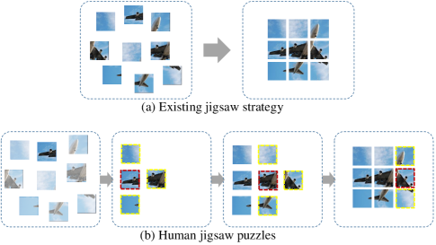
Figure 1: The difference between existing jigsaw strategy and human jigsaw puzzles. Fig. 1(a) presents the existing jigsaw methods which almost focus on learning permutation and sorting with pixels. Human jigsaw puzzles first use one piece as a benchmark to consider the parts around it which is learning splicing and linking by prior image semantics understanding as shown in Fig. 1(b).

Image clustering, as a fundamental task in computer vision, aims to grouping similar images together based on their visual representations without annotations. As an unsupervised learning task, it evolves around the pivotal task of extracting discriminative image representations. With the advent of deep learning progress, particularly pre-training large-scale vision models in the last two years, researchers have made substantial advancements in image clustering, achieving superior performance compared to traditional methods that relied on handcrafted features [1, 2, 3, 4, 5].

Although deep learning models have revolutionized the field of computer vision by automatically learning hierarchical representations from raw images, the limitations are still existed in the image clustering field. First, these supervised learning visual models, i.e, CNN-based [6] and Transformer-based [7], are trained from the global labels. They primarily focus on differentiating relationships between entire images, while overlooking the internal structure of individuals. However, the internal structural relationships within images hold crucial significance for image representation. Moreover, the annotated label in image classification or object recognition training process tend to be a single word, which is overly simplistic. Image representations trained on such simple labels only capture the mapping relationship between images and basic labels, failing to provide nuanced discriminative representations. Consequently, directly utilizing image features extracted from these visual models for image clustering tasks remains insufficient.

To this end, we address the limitations of existing visual models in the context of image clustering. Self-supervised learning has proven to be an effective approach for learning internal features from data. As a pretext task of self-supervised learning, jigsaw puzzle [8] has shown the ability of exploring the internal structure relationships within images. As shown in Fig 1(a), by breaking an image into several patched and then reconstructing it, the Jigsaw puzzle task aims to capture the internal relationships and spatial dependencies between different regions by shuffling and rearranging all puzzle pieces simultaneously. The achievements from the subsequent researches [9, 10] demonstrate its potential in uncovering the hidden structural patterns within images. Although Jigsaw puzzle is inspired by human jigsaw solving, the existing Jigsaw puzzle algorithm does not necessarily replicate the exact process of human. In human jigsaw solving, we typically start by identifying a specific puzzle piece and then proceed to locate neighboring pieces around it. This step-by-step approach allows for a gradual construction, focusing on a subset of pieces at a time, as shown in Fig. 1(b). Comparing with the Jigsaw puzzle pretext task, the human solving process is a more sequential and incremental understanding of image structure. In our previous work [11], we have preliminarily explored the grid feature based on jigsaw strategy for image clustering and demonstrated its prominent performance via experiments. In this paper, we further elaborate the breakthrough improvement from pixels on the low-level statistics to features on the high-level perception.

In recent years, the integration of vision and language has emerged as a promising research direction in computer vision. Vision and language pre-training models, such as the Contrastive Language-Image Pre-training (CLIP) [12], utilizes large-scale datasets of images and their associated textual descriptions to learn a joint embedding space. By leveraging the joint embedding space provided by CLIP, image clustering algorithms can benefit from the enhanced cross-modal representation for richer and more nuanced training labels to foster the development of highly discriminative image representations. In this paper, we replace the convolutional image representation with cross-modal CLIP features to investigate how the cross-modal representation can improve the effectiveness and efficiency of image clustering algorithms. We find that this cross-modal representation not only enhances the accuracy of image clustering but also significantly improves the convergence speed of the clustering algorithms. This acceleration in convergence not only improves the efficiency of image clustering but also facilitates the scalability of the clustering algorithms to larger datasets.

To sum up, we propose a new perspective on image clustering which combines pretrained CLIP visual encoder to extract the prior features and jigsaw strategy to improve clustering performance called pretrain-based Grid Jigsaw Representation (pGJR). Specifically, we first employ a pretrained visual-language model CLIP as a visual extractor to obtain visual representation. Then, we propose the jigsaw supplement method expanded by our previous work GJR [11] to fit pretrained representations in training. CLIP pretrained representations provide powerful prior features and GJR as location attention maps supports more refined adjustment. It is intuitively considered that the nearly finished puzzle with bits of patches in error position or vacancy will not be shuffled again but modify some local positions. We evaluate the effectiveness of our methods for the image clustering benchmarks and provide sufficient ablation study and visualization results.

Our main contributions can be summarized as follows:

• We propose a new perspective on image clustering which combines pretrained CLIP visual encoder and jigsaw strategy to improve clustering performance named pretrain-based Grid Jigsaw Representation (pGJR) and verify it on the five benchmarks where the results show the great performance on image clustering task.

• We design a subhuman jigsaw puzzle module to the middle-level visual feature which as a plugin can mine the semantic information on a higher level representation learning. It has strong generalization in both of deep CNN training and combined pretrained model.

• We exploring the cross-modal representation in the context of image clustering where pretrained CLIP provide mature and learning-friendly representations to improve the performance and efficiency for clustering training.

The remainder of this paper is arranged as follows. Section II mainly reviews the related work about deep clustering, self-supervised learning and grid feature. Section III introduces our proposed method named Grid Jigsaw Representation with motivation and algorithm. Section IV proposes a new perspective on clustering about pre-trained model and jigsaw supplement with pretrain-based visual extractor CLIP, pretrain-based Grid Jigsaw Representation and clustering training process. Section V presents experimental details, results and ablation study with visualization. Section VI contains the concluding remarks.

II Related Work

II-A Deep clustering

Deep clustering [13, 14] as a fundamental and essential research direction, mainly leveraged the power of deep neural networks to learn high-level features incorporating traditional clustering methods [15]. The concept of spectral clustering [16] was introduced to set up input of positive and negative pairs according to calculate their the Euclidean distance with classical k-means and promoted many related researches [17, 18, 19, 20, 21] to obtain competitive experimental results. Xu et al. [22] introduced a novel approach that combines contrastive learning with neighbor relation mining, updated alternately during forward and backward propagation, which acquires the capability to capture intricate relationships between images, leading to achieve more accurate image clusters and more precise semantic understanding. Li et al. [23] demonstrated that data augmentation can impose limitations on the identification of manifolds within specific domains, where neural manifold clustering and subspace feature learning embedding should surpasses the performance of autoencoder-based deep subspace clustering. Starting with a self-supervised SimCLR [24], recent visual representation learning methods [25, 26, 27] have achieved great attention for clustering. Tsai et al. [28] leveraged both latent mixture model and contrastive learning to discern different subsets of instances based on their latent semantics. By jointly representation learning and clustering, Do et al. [29] proposed a novel framework to provide valuable insights into the intricate patterns at the instance level and served as a clue to extract coarse-grained information in objects.

II-B Self-supervised Learning

Self-supervised learning has been a thriving field of research for visual representation learning, which aims to extract key semantic information and discriminative visual feature from images. As one of the pretext tasks, jigsaw puzzles [8, 30] trained the network to reassemble the image tiles from a set of permutations and there was a strong knowledge association between patches of the puzzles. Instead of regarded jigsaw puzzles as a independent pretext task, some studies follow the logic of its pattern generalized to more downstream tasks by self-supervised training such as image classification [31, 32] and other applications as follow: Abdolahnejad et al. [33] used the obvious distribution characteristics of human face to train the patches with generative adversarial networks, which can generate and piece together new patches to produce high-quality face images. Chen et al. [10] proposed a jigsaw clustering for self-supervised learning with the disturbed patches as the output and the original image as the target from both intra-image and inter-images.

Furthermore, typical self-supervised architectures inspired representation learning research. Wu et al. [19] learned the feature representation by requiring only features with distinguish individual instances, in order to capture the obvious similarity between instances. Chen et al. [24] proposed a simplified contrastive self-supervised learning framework with learnable nonlinear transformation and effective composition of data augmentations. Siamese architectures for unsupervised representation learning aim to maximize the similarity between two augmentations of one image. Chen et al. [34] proposed a hypothesis on the implication of stop-gradient to prevent collapsing. Zbontar et al. [35] provided a conceptually simple method applying redundancy-reduction to benefit from high dimensional embedding. Bardes et al. [36] based on covariance criterion proposed variance term to apply both branches of the architecture preventing informational collapse. To address the lack of explicit modeling between visible and masked patches, the context autoencoder [37] was proposed to overcome limited representation quality through combination of masked representation prediction and masked patch reconstruction.

II-C Grid Feature

The discussion of grid features mainly existed in object detection task [38, 39] compared with region features about network design and performance. Since Jiang et al. [40] verified the grid feature performance on the visual-language task, grid feature has received more attention in visual representation. Referring to the mask words in sentence in natural language processing [41], many researches especially based on transformer structure [42, 43] masked grid units of image to learn the connections between pixels. Huang et al. [44] passed images directly into feature module pixel by pixel to learn local feature relationships in details and Dosovitskiy et al. [7] proved that images are worth to be divided into 256 patches for vision recognition. He et al. [45] designed powerful masked autoencoders by randomly covering the grids of the input image and reconstructing the missing pixels. Wa et al. [46] used grid partition and decision-graph to quickly identify the clustering center to enhance robust. However, many of these successfully used the grid pixels rather than features to carry out the large-scale pre-training to learn the relationship and almost cost huge computing resources.

III Grid Jigsaw Representation

Figure 2: The framework illustration of proposed GJR where Fig. 2(a) is pixel-based version and Fig. 2(b) is feature-based one. There are both five steps about CNN Extraction, Block Division, Grid Division, Linear Regression and Reconstruction, but in different orders.

In this section, we introduce the Grid Jigsaw Representation (GJR) methods with two parts: Motivation and Algorithm. It is a complete exposition for GJR which we propose in our previous work [11]. The Motivation introduce a improved insight for GJR why we propose a new kind of jigsaw strategy and its conception from pixel to feature (our previous work just preliminary attempt on grid feature). The Algorithm shows the specific details for GJR where framework is shown in Fig. 1 and algorithm steps are shown in Alg. 1.

III-A Motivation

Unlike supervised learning, unsupervised learning requires a global constraint based on training samples without ground truth labels. In addition to constraints through loss functions [24], self-supervised learning can also be considered to design diverse network structures according to the characteristics and properties in data or task. It would be abstract and ingenious which aims imitate human logic. Jigsaw strategy [8] as one of self-supervised learning methods mimic human jigsaw puzzles in analysis, understanding, and operation of image patches. However, as mentioned before and shown Fig. 1, there are still different between the existing jigsaw strategies and human jigsaw puzzles. The main distinguishing factor is that most of existing jigsaw strategies and its extend versions are all based on the raw image patches which concentrate on the low-level statistics, such as structural pattern and texture. In the deep neural networks, the feature maps on the top layer of neural networks imply high-level clues for visual representation while not suit for human intuitive perceptual. But it should not be a reason to discard operation on high-level features, just like it is still much unknown about how the human brain learns things. Thus, we consider to implement the jigsaw strategy on the deep layer features and compare with pixels.

Our previous work [11] has made a preliminary attempt and module of our jigsaw strategy is referred as Grid Jigsaw Representation (GJR) in this paper. GJR is inspired by jigsaw puzzles and grid feature. Given the pieces of jigsaw puzzles, people tend to infer the position of each puzzle piece from the overall structure of the picture. Jigsaw puzzles imply a certain prior knowledge: the closer the distance is, the stronger the relevance of patches will be. The human learning clues of solving jigsaw from whole image provided by surrounding patches are more than learning by patch itself. According to this view, we assume that the computer learning clues of visual representation from whole feature provided by surrounding feature grids are more than learning by grid itself. In another word, for a whole grid feature map separated into blocks, the information of the grids adjacent to the one is more valuable than itself in the same block. So, we provide GJR which replaces grid with surrounding grids in the block to learn visual representation. The recent works like BERT [41] or MAE [47] have the similar idea by using masked to predict in pretraining. We should emphasize that our jigsaw is different from them, because there is no prediction and every patch is given. So it is more similar to the evidence-based association which is equivalent to seeing a complete image.

We note that an intuitive presentation may not be enough to capture feature-based advantages or prove that jigsaw strategy would be better used on features rather than pixels. In this paper, we expand GJR into pixels and demonstrate advantage of GJR based on features through experimental comparison.

III-B Algorithm

Fig. 2 shows the framework of GJR respectively based on pixels and based on features. There are five steps in GJR: CNN Extraction, Block Division, Grid Division, Linear Regression (LN) and Reconstruction. It can be found that only CNN Extraction is in a different order. GJR based on features first extracts image high-level features and then implement jigsaw operation to get new representation. While GJR based on pixels is the opposite which extracts the features last. Since the steps are basically the same, we only introduce GJR based on features to show the specific algorithm.

Algorithm 1 Grid Jigsaw Representation

Input: image $x$

Output: Jigsaw representation $X^{*}$

1:  $X^{{}^{\prime}}=CNN(x)$ //CNN extraction output is $n$ dimension feature maps.

2:  $X^{{}^{\prime}}_{G}=Grid(X^{{}^{\prime}}),$ //$Grid(\cdot)$ operation as follow: $X^{{}^{\prime}}_{G}=\{B^{{}^{\prime}}_{i}\},i\in[1,m]$ //Block division comes to $m$ blocks and every block is $l\times l$ feature.$B^{{}^{\prime}}_{i}=\{g^{{}^{\prime}}_{j}\},j\in[1,l]$//Grid division sorts each block by row.

3:  for $i=1$ to $m$ do

4:     $B^{{}^{\prime}}_{i}=\{g^{{}^{\prime}}_{j}\},j\in[1,l]$

5:     for $j=1$ to l do

6:        $g^{*}_{j}$ = LN($B^{{}^{\prime}}_{i}$, without $g^{{}^{\prime}}_{i}$) //Reconstruction of local feature by Linear Regression (LN).

7:     end for

8:     $B^{*}_{i}=\{g^{*}_{j}\},j\in[1,l]$

9:  end for

10:  $X^{*}=\{B^{*}_{i}\},i\in[1,m]$

11:  return $X^{*}$

As shown in Alg. 1, given an image $x$ as input, feature maps $X^{{}^{\prime}}$ is extracted by deep Convolutional Neural Network (CNN), which preserves CNN output dimension size $n$.

$$X^{{}^{\prime}}=CNN(x)$$ (1)

We performed GJR on feature maps $X^{{}^{\prime}}$. Specifically, $X^{{}^{\prime}}$ is divided into $m$ blocks and each block has $l\times l$ size which should meet split size $n=m\times l\times l$. It is to ensure that the grid of image feature in each block is properly close and relevant. In order to reduce the computational difficulties caused by the edge influence and reduce the complexity of the algorithm, we define row $g^{{}^{\prime}}_{j}$, $j\in[1,l]$ as a unit grid for each block $B^{{}^{\prime}}_{i},i\in[1,m]$. Thus, we obtain the grid feature maps, regionalized and orderly permutation as follow definition:

$$X^{{}^{\prime}}_{G}=Grid(X^{{}^{\prime}})$$ (2)

where set $X^{{}^{\prime}}_{G}=\{B{{}^{\prime}}_{i}\},i\in[1,m]$, set $B{{}^{\prime}}_{i}=\{g^{{}^{\prime}}_{j}\},j\in[1,l]$. $B{{}^{\prime}}_{i}$ is block and $g{{}^{\prime}}_{j}$ is grid. $Grid(\cdot)$ just implements division operation and has not change $X^{{}^{\prime}}$, so $X^{{}^{\prime}}_{G}$ keeps its value. In this way, we can assume that every unit grid in each block has a strong semantic correlation because of its close distance. We extract and integrate other grids except $g^{{}^{\prime}}_{j}$ in block $B_{i}$ to reconstruct $g^{*}_{j}$. $g^{*}_{j}$ as unit grid of jigsaw representation has the same size to $g^{{}^{\prime}}_{j}$ with linear regression:

$$g^{*}_{j}=\sigma(\omega_{j}(\sum_{g^{{}^{\prime}}\neq g^{{}^{\prime}}_{j}}^{B_{i}}g^{{}^{\prime}})+\delta_{j})$$ (3)

where $\omega_{j}$ is trainable weight and $\delta_{j}$ is vector bias. $\sigma$ is the ReLU activation function. Then the new representation $X^{*}$ is reconstructed by all $g^{*}_{j}$. The representation $X^{\prime}$ with $B^{{}^{\prime}}_{i}$ as block, $g^{{}^{\prime}}_{j}$ as unit grid is transformed into the jigsaw representation $X^{*}_{i}$ with $B^{*}_{i}$ as block, $g^{*}_{j}$ as grid. Note that our reconstruction just work in the forward propagation and has not predict target for it, which is mainly different from other methods. We need to emphasize the practical significance of $B^{*}_{i}$ totally different from $B^{{}^{\prime}}_{i}$. $X^{*}$ holds a higher dimension which integrates the relationship of information in the graphic area. Each grid feature in $B^{*}_{i}$ is a collection of adjacent information of the original grid feature in $B^{{}^{\prime}}_{i}$.

IV Pre-trained model and jigsaw supplement

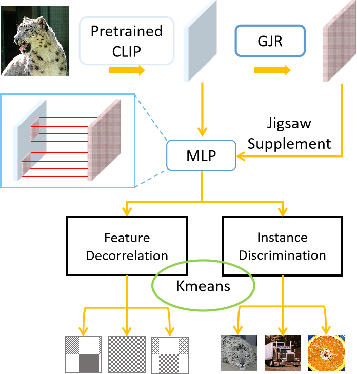
Figure 3: The framework illustration of proposed pGJR consisted of CLIP-based representation structure and jigsaw supplement for image clustering. The representation learning includes jigsaw feature network in forward prorogation and clustering constraint optimization in backward propagation.

In this section, we introduce the new perspective on image clustering where pretrained image-text model CLIP [12] is used as a visual extractor to replace CNN for training. This pattern can efficiently improve the convergence speed of clustering. Moreover, we provide pretrain-based Grid Jigsaw Representation (pGJR) which can be a supplement to further improve the clustering performance in such pattern. Finally, we introduce the training process for image clustering. The framework is shown in Fig. 3.

IV-A Pretrain-based visual extractor CLIP

We employ a pretrained visual-language model CLIP [12] as a visual extractor to replace the CNN extractor in Section III. It is pretrained representation from CLIP visual encoder which as prior feature. We first propose CLIP(only) as our new baseline which provides better and faster clustering representations.

Given image x as input, representation $X_{C}$ is extracted by pretrained CLIP. The output here inherits the dimension 768 from the CLIP final layer:

$$X_{c}=CLIP(x)$$ (4)

Then, one MLP is used to transform features from 768 to n where we set it the same dimension as final GJR’s $X^{*}$ for clustering. In this way, MLP is simply a linear layer as LN:

$$\hat{X_{c}}=LN(\textbf{W}_{c}X_{c}+\Delta_{c})$$ (5)

where $\textbf{W}_{c}$ is trainable weight matrix and $\Delta_{c}$ is vector bias group. Subsequent experiments will prove pretrained representation $\hat{X_{c}}$ as initial value with powerful prior information which provides efficient convergence speed and improves baseline of image clustering. We find that it is already state-of-the-art on most of our test dataset but it also shows some limitations in fine-grained ability which will be discussed later in the experiment section.

IV-B Pretrain-based Grid Jigsaw Representation

Moreover, we expand our GJR methods with CLIP feature called pGJR. Get CLIP representation $X_{C}$ first. Then, pGJR handles $X_{C}$ like the proccess in Alg. 1 to obtain $X^{*}_{C}$:

$$X^{*}_{C}=GJR(X_{C})$$ (6)

It is same to CLIP(only) that the representation should be transformed from 768 to n through a MLP. But there is little different and not direct use $X^{*}_{C}$:

$$\hat{{X^{*}_{c}}}=LN^{*}(\textbf{W}^{*}_{c}[X_{c}+\sigma_{c}(X^{*}_{C})]+\Delta^{*}_{c})$$ (7)

where $\textbf{W}^{*}_{c}$ is trainable weight matrix and $\Delta^{*}_{c}$ is vector bias group. We add the ReLU activation function $\sigma_{c}$ here where $\sigma_{c}X^{*}_{C}$ will be not a reconstruction representation but a region attention to replenish $X_{C}$. It is considered that CLIP as a mature visual feature extractor provides powerful prior information to generate representation. Thus, it is no use to global reconstruction to disrupt again. Turning to jigsaw puzzles, people will not shuffle afresh the jigsaw when it comes to finish with bits of patches in error position. Thus, only the local features need to be strengthened or modified. Finally, we use $\hat{{X^{*}_{c}}}$ as pGJR output for clustering.

IV-C Clustering

Clustering task requires to distinguish objects through the representation of the image itself. It should not only focus on the relationship with adjacent regions in the sample, but also should distinguish the similar features in different samples. We think that GJR provide a great visual representation method to learning the image in clustering task and its motivation aims to learn the splicing and linking with understanding the visual semantics through jigsaw strategy.

We apply the state-of-the-art levels representation learning method IDFD [21] with simple k-means to obtain the clustering results, where the Instance Discrimination [19] to capture the similarity between instances and Feature Decorrelation [21] to reduce correlations within features. GJR and pGJR are the same to add as the module following the visual representation features. Given unlabeled dataset $\{x_{i}\}^{n}_{i=i}$, every image $x_{i}$ is learned and reduced dimension by fully connected layer to obtain Jigsaw representation $X^{*}_{i}$. Then define the whole representation set $V=\{v_{i}\}^{n}_{i=1}=\{X^{*}_{i}\}^{n}_{i=i}$ to be set with a predefined number of clusters $k$.

Given $x_{i}$ corresponding representation $v_{i}$, Instance Discrimination controls data $x_{i}$ classified into the $i$th class. The $v_{i}$ as weight vector can be calculated with the probability of $v$ being assigned into the $i$th class:

$$P(i|v)=\frac{exp(v^{T}_{i}v_{i}/\tau_{1})}{\sum^{n}_{j=1}{exp(v^{T}_{j}v_{i}/\tau_{1}})}$$ (8)

where $v^{T}_{i}v_{i}$ is to evaluate how match degree $v_{i}$ with the $j$th class, and $\tau_{1}$ is a temperature parameter. Then the objective function $L_{I}$ of instance discrimination as follow:

$$L_{I}=-\sum^{n}_{i}{log(\frac{exp(v^{T}_{i}v_{i}/\tau_{1})}{\sum^{n}_{j=1}{exp(v^{T}_{j}v_{i}/\tau_{1}})})}$$ (9)

Feature Decorrelation provides constraints on features between different images and fits GJR with the backward propagation. It defines a set of latent vectors $F=V^{T}=\{f_{l}\}^{d}_{l=1}$. Unlike with (8), the new constraint is transformed to:

$$Q(l|f)=\frac{exp(f^{T}_{l}f_{l}/\tau_{2})}{\sum^{d}_{m=1}{exp(f^{T}_{m}f_{l}/\tau_{2}})}$$ (10)

where $Q(l|f)$ is similar to $P(i|v)$ but the implication of the transposed feature $f$ will be completely different semantic information from $v$. $\tau_{2}$ is the another one temperature parameter. And objective function $L_{D}$ of feature decorrelation as follow:

$$L_{D}=-\sum^{m}_{l}{log(\frac{exp(f^{T}_{l}f_{l}/\tau_{2})}{\sum^{d}_{m=1}{exp(f^{T}_{m}f_{l}/\tau_{2}})})}$$ (11)

To sum up the combination of $L_{I}$ and $L_{D}$, the whole objective function is shown as:

$$L=L_{I}+\alpha L_{D}$$ (12)

where $\alpha$ controls the distribution balance of both.

V Experiments

In this section, we first introduce the datasets and evaluation metrics. Then, we show and analyze the main results for GJR and pGJR respectively. By contrast, representation ability of GJR is obvious and convergence efficiency for pGJR is emphasized. Finally, ablation study demonstrates eneralizability performance and shows the feature representations distribution.

V-A Datasets and Metrics

TABLE I: Statistics of different datasets.

Dataset	Images	Clusters	Image size
CIFAR-10	50,000	10	32 × 32 × 3
CIFAR-100	50,000	20	32 × 32 × 3
STL-10	13,000	10	96 × 96 × 3
ImageNet-10	13,000	10	96 × 96 × 3
ImageNet-Dog	19,500	15	96 × 96 × 3

Following the five common used benchmarks, we conduct unsupervised clustering experiments on CIFAR-10 [48], CIFAR-100 [48], STL-10 [49], ImageNet-10 [50], ImageNet-Dog [50]. We summarize the statistics and key details of each dataset in Table I where we list the numbers of images, number of clusters, and image sizes of these datasets. Specifically, the training and testing sets of dataset STL-10 were jointly used and images from the three ImageNet subsets were resized as shown. We follow the three metrics: standard clustering accuracy (ACC), normalized mutual information (NMI), and adjusted rand index (ARI). The higher the percentage of these three metrics, the more accurate clustering assignments. Every experiment result is trained on two NVIDIA 3060 for GJR and one enough for pGJR.

V-B GJR Results

TABLE II: Hyperparameter setting for GJR of different datasets. $\eta_{0}$ is initial learning rate. Epoch(gamma) shows which epoch to reduce learning rate and its ratio.

Dataset	$\eta_{0}$	Epoch(gamma)	Block	Grid
CIFAR-10	2e-2	800/1300/1800(0.1)	8	4 × 4
CIFAR-100	3e-2	800/1800(0.1)	2	8 × 8
STL-10	3e-2	800/1200(0.1)	2	8 × 8
ImageNet-10	3e-2	—	2	8 × 8
ImageNet-Dog	3e-2	600/950/1300/1650(0.1)	8	4 × 4

TABLE III: Evaluating clustering results (%) on five datasets compared with advanced methods for GJR. Our performance is trained on ResNet18 as backbone. The listed meathods are Mostly cited in our previous work [11]. The best results are highlighted in blod and the second are in orange

Dataset(%)	CIFAR-10	CIFAR-100	STL-10	ImageNet-10	ImageNet-Dog
Metric	ACC  NMI  ARI	ACC  NMI  ARI	ACC  NMI  ARI	ACC  NMI  ARI	ACC  NMI  ARI
DEC [51]	30.1  25.7  16.1	18.5  13.6  5.0	35.9  27.6  18.6	38.1  28.2  20.3	19.5  12.2  7.9
DAC [13]	52.2  39.6  30.6	23.8  18.5  8.8	47.0  36.6  25.7	52.7  39.4  30.2	27.5  21.9  11.1
DCCM [14]	62.3  49.6  40.8	32.7  28.5  17.3	48.2  37.6  26.2	71.0  60.8  55.5	38.3  32.1  18.2
IIC [52]	61.7  51.1  41.1	25.7  22.5  11.7	59.6  49.6  39.7	—— —— ——	—— —— ——
PICA [53]	69.6  59.1  51.2	33.7  31.0  17.1	71.3  61.1  53.1	87.0  80.2  76.1	35.2  35.2  20.1
DRC [54]	72.7  62.1  54.7	36.7  35.6  20.8	74.7  64.4  56.9	88.4  83.0  79.8	38.9  38.4  23.3
MiCE [28]	83.5  73.7  69.5	42.2  43.0  27.7	72.0  61.3  53.2	—— —— ——	39.0  39.0  24.7
IDFD [21]	81.5  71.1  66.3	42.0  42.6  26.4	75.6  64.3  57.5	95.4  89.8  90.1	59.1  54.6  41.3
CRLC [29]	79.9  67.9  63.4	42.5  41.6  26.3	81.8  72.9  68.2	85.4  83.1  75.9	46.1  48.4  29.7
NNCC [22]	81.9  73.7  ——	43.8  42.1  ——	72.5  61.6  ——	75.1  68.3  ——	40.1  37.2  ——
NMCE [23]	83.0  76.1  71.0	43.7  48.8  32.2	72.5  61.4  55.2	90.6  81.9  80.8	39.8  39.3  22.7
GJR(pixels)	79.8  69.8  63.8	36.8  37.3  22.3	71.4  60.0  51.9	87.5  79.0  75.6	44.2  41.0  25.7
GJR(features)	83.7  75.0  70.2	46.1  45.9  29.6	78.2  68.9  59.6	96.2  91.3  91.9	62.2  58.9  44.3

For the GJR results, We adopted the best comprehensive effect ResNet18 [6] as the basic neural network architecture for GJR and easy reproduced clustering method strategy with IDFD [21] and kmeans. Our experimental settings and data augmentation strategies are just in accordance with IDFD [21]. We listed the important parameters settings like 128 batch sizes and output feature dimension size $n=128$ from ResNet18. The weight $\alpha=1$ is all fixed according to the orders of magnitudes of losses. Temperature parameters are set as $\tau_{1}=1$ and $\tau_{2}=2$. The parameters in GJR module, such as block number $m$ and grid number $l$, are set according to the size of feature maps with specific deep convolutional neural network. The size of grid tensor $n$ will be certain after the two values product of $m$ and $l$ are determined $n=m\times l\times l$. For example, $m=8$ and $n=4$ when $n=128$. Our main hyperparameters for GJR are grid numbers which to control $m$ and $l$ and learning rate to control training rhythm as shown in Table II.

Table III shows GJR performance compared with other advanced clustering methods where we almost keep the same results in our previous work [11]. The result on ImageNet-Dog gets further improvement with change grid number 8 to 4. Our results for GJR based on features obtained the best and second performance in these clustering methods. Due to highly focus on the image sample itself and distinction, GJR shows the best performance on higher-image-quality ImageNet-10 and ImageNet-Dog. Except IDFD [21] which we follow and use the same clustering strategy, there are all more than $5\%$ improvement on ImageNet-10 and $10\%$ on ImageNet-Dog in three metrics with other methods. GJR gets the best ACC on CIFAR-10 and CIFAR-100 where NNCC [22] and NMCE [23] are higher on NMI and ARI. The result on STL-10 is outstood by CRLC [29]. It is reflected the performance difference of clustering methods which are mainly driven by data. We also test our GJR based on pixels although we think it may not make sense from the beginning design and the experiment result also prove it. We emphasize GJR mimic human jigsaw logic which requires prior processing features rather than low-level pixels.

V-C pGJR Results

TABLE IV: Hyperparameter setting for pGJR of different datasets.$\eta_{0}$ is initial learning rate. $\eta_{1}$(epoch) is learning rate of second stage and its epoch.

Dataset	$\eta_{0}$	$\eta_{1}$(epoch)	Block	Grid
CIFAR-10	5e-1	1e-2(75)	8	4 × 4
CIFAR-100	2e-2	2e-3(75)	2	8 × 8
STL-10	2e-2	2e-3(100)	2	8 × 8
ImageNet-10	5e-2	1e-3(30)	8	4 × 4
ImageNet-Dog	5e-2	5e-3(45)	2	8 × 8

TABLE V: Evaluating clustering results (%) on five datasets compared state-of-the-art. Our performance is trained with pretrained frozen model CLIP. The best results are highlighted in blod and the second are in orange. References to grey backgrounds use pseudo-tags or semi-supervised algorithms.

Dataset(%)	CIFAR-10	CIFAR-100	STL-10	ImageNet-10	ImageNet-Dog
Metric	ACC  NMI  ARI	ACC  NMI  ARI	ACC  NMI  ARI	ACC  NMI  ARI	ACC  NMI  ARI
SCAN [55]	88.3  79.7  77.2	50.7  48.6  33.3	80.9  69.8  64.6	——  ——  ——	——  ——  ——
IMC-SwAV [56]	89.7  81.8  80.0	51.9  52.7  36.1	85.3  74.7  71.6	——  ——  ——	——  ——  ——
TCL [57]	81.9  88.7  78.0	52.9  53.1  35.7	79.9  86.8  75.7	87.5  89.5  83.7	62.4  63.9  50.3
SPICE [27]	92.6  86.5  85.2	53.8  56.7  38.7	93.8  87.2  87.0	95.9  90.2  91.2	67.5  62.7  52.6
MiCE [28]	83.5  73.7  69.5	42.2  43.0  27.7	72.0  61.3  53.2	—— —— ——	39.0  39.0  24.7
IDFD [21]	81.5  71.1  66.3	42.0  42.6  26.4	75.6  64.3  57.5	95.4  89.8  90.1	59.1  54.6  41.3
PCL [58]	80.2  87.4  76.6	52.8  52.6  36.3	41.0  71.8  67.0	84.1  90.7  82.2	44.0  41.2  29.9
CRLC [29]	79.9  67.9  63.4	42.5  41.6  26.3	81.8  72.9  68.2	85.4  83.1  75.9	46.1  48.4  29.7
NNCC [22]	81.9  73.7  ——	43.8  42.1  ——	72.5  61.6  ——	75.1  68.3  ——	40.1  37.2  ——
NMCE [23]	83.0  76.1  71.0	43.7  48.8  32.2	72.5  61.4  55.2	90.6  81.9  80.8	39.8  39.3  22.7
GJR	83.7  75.0  70.2	46.1  45.9  29.6	78.2  68.9  59.6	96.2  91.3  91.9	63.7  61.0  47.0
CLIP(only)	87.0  79.0  71.5	57.2  56.2  38.1	97.6  94.1  94.7	98.2  95.6  96.0	53.6  54.5  42.3
pGJR	87.5  79.3  72.6	58.3  58.2  38.2	97.9  94.7  95.3	98.8  96.9  97.4	57.8  56.8  44.3

We keep clustering method strategy with IDFD [21] and kmeans. First about CLIP(only), the backbone Resnet18 was replaced by pretrained CLIP [12] to extract image feature and a Linear layer was added as MLP. Specifically, it means that CLIP as visual extractor is frozen and just to train the one Linear layer parameters. The experimental settings and data augmentation strategies are same with GJR which we do not repeat. There are just the change from Linear layer to GJR module as Alg. 1 shown for pGJR. Hyperparameters for pGJR to improve training performance are adjusted as shown in Table IV.

We first compare the convergence efficiency between GJR and pGJR in Fig. 4 which is the most intuitive to tell why we do and expand our work. It can found that GJR with initial ResNet18 requires nearly 1200 epochs to start converging and even 2000 epoch to approach best performance in our experiment. But pGJR with pretained CLIP reaches and exceeds the level in just 150 epochs. The training time for each epoch is mostly same for GJR and pGJR. Pretrained models like CLIP do not require much gpu memory and use for free. Meanwhile, clustering tasks do not require large models with very good performance because unsupervised learning for unlabeled samples still need unsupervised algorithms to train.

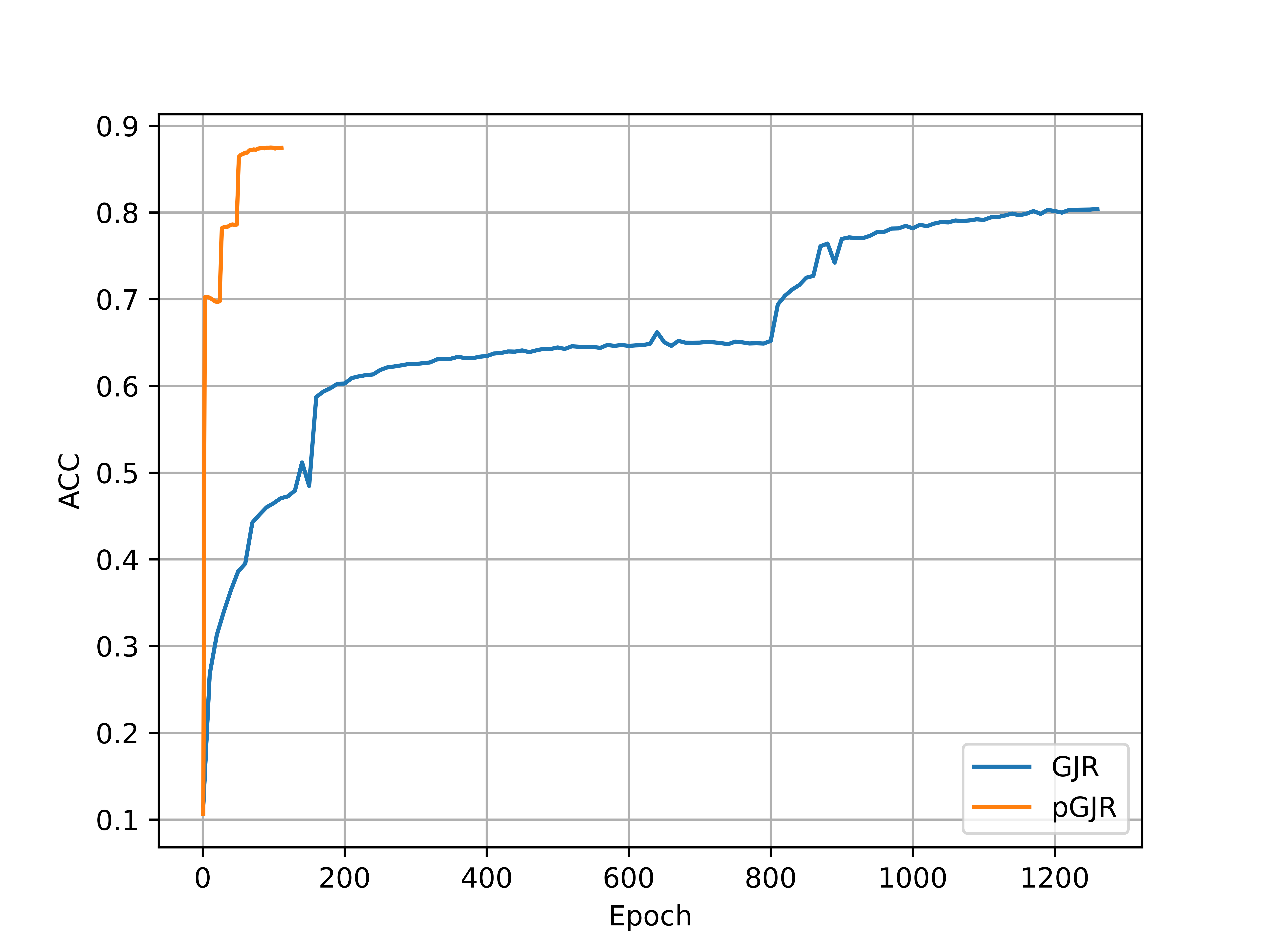
Figure 4: Convergence efficiency and performance compared with GJR and pGJR on CIFAR-10.

Table V shows pGJR performance with recent advanced clustering methods. Our proposed results by CLIP(only) and pGJR all just use kmeans for unsupervised clustering and train few linear layers parameters with in low training cost. Thus, the SOTA methods about SCAN [55], IMC-SwAV [56], TCL [57] using pseudo-tags which list on the paper-with-code and SPICE [27] adopting semi-supervised algorithms are set in gray background are not compared in Table V. It can be found that our proposed method mostly obtained best and second performance. Even our pGJR are SOTA methods and exceed semi-supervised algorithms SPICE [27] on CIFAR-100, STL-10 and ImageNet-10. Compared with traditional methods, It is not surprising that our pretrained strategy has improved distinctly as the results coloured by orange. Then, introduced GJR module makes further achievement from CLIP(only). However, we find that pretrained strategy is failed in fine-grained dataset ImageNet-Dog. Considered CLIP training, the matching pair with dog is ’The photo of a dog’ which does not pay attention on the difference in dog kinds. So the representations provided by pretrained CLIP are unsatisfactory on ImageNet-Dog. Although pGJR remedies NMI and ARI just in a short-stage training by powerful distinction from samples, we still suggest using GJR based on ResNet to train on fine-grained dataset rather than pretrained CLIP.

V-D Ablation Study

TABLE VI: Clustering results (%) on various deep network architectures on CIFAR-10. Net(only) means just backbone as framework.

Backbone	ResNet18	VGG16	DenseNet	ResNet34	ResNet152	Pretrained CLIP
Metric	ACC  NMI  ARI	ACC  NMI  ARI	ACC  NMI  ARI	ACC  NMI  ARI	ACC  NMI  ARI	ACC  NMI  ARI
Net(only)	82.1  72.8  67.0	52.1  43.0  30.9	50.0  39.4  29.1	82.7  73.4  68.4	83.4  74.7  69.7	87.3  79.3  72.2
Net + GJR	83.7  75.0  70.2	54.1  44.6  33.1	54.0  43.8  34.0	84.0  75.2  70.5	84.0  75.3  70.5	87.5  79.3  72.6
Up(+)	1.7    3.2    2.7	2.0    1.6    2.2	4.0    4.4    4.9	1.3    1.8    2.1	0.6    0.6    0.8	0.2    0.2    0.4

Firstly, it is underlying to embody generalizability performance for GJR. We fix random seeds and keep each parameter following the setting. There are three different convolutional networks used to test: ResNet [6], VGG [59] and DenseNet [60] and more deep layers for ResNet. Although, pGJR use the pretrained CLIP to extract the feature without training backbone, we think it is another form to prove scope of GJR application. As shown in Table VI, GJR module improves the performance of all kinds listed networks without exception. Simultaneously, we consider that GJR excavates the potential of CNN for image feature learning especially in shallow layers model. Performance continues to increase when deepening the ResNet depth for Net(only). But GJR trains all depth ResNet approaching to the same outstanding performance. ResNet18 with GJR has already better than ResNet152 Net(only) at the same epoch which greatly reduces computing costs.

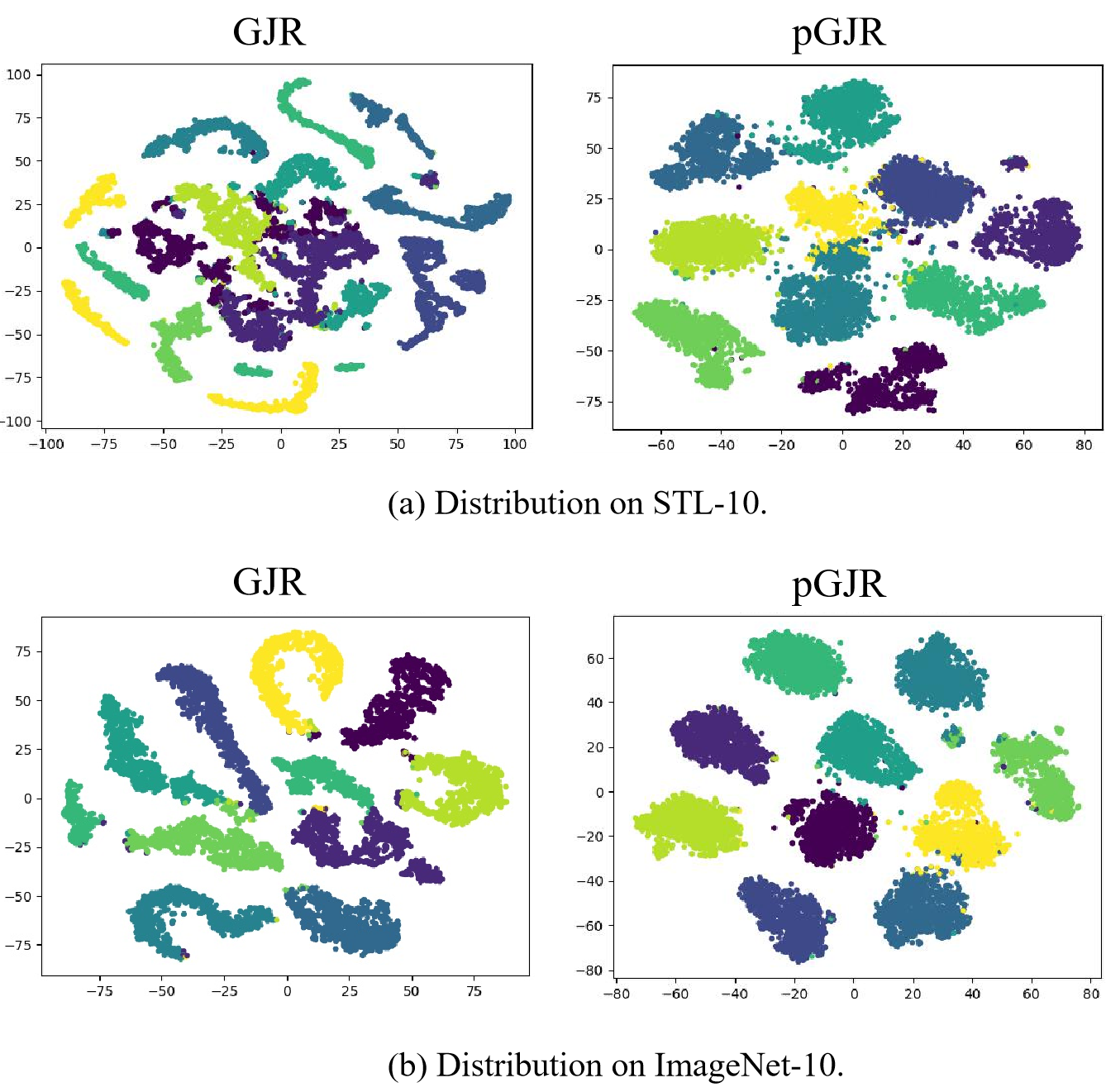
Figure 5: Visualization of clustering feature representations distribution compared with GJR and pGJR.

Then, we show the clustering feature representations distribution compared with GJR and pGJR in Fig. 5 on STL-10 and ImageNet-10. The distributions show the preference for clustering between GJR and pGJR. It is clearly that every kind of clusters is compact and narrow for GJR which determines cleaner boundaries and distances between distinguishable categories due to long-period training. But the same species may be distributed in more than one area such as the yellow for GJR on STL-10 in Fig. 5(a) left. pGJR shows more evenly distributed clusters with the highest metrics. There are sufficiently distinct contours and obvious clustering centers with a few hard samples failed.

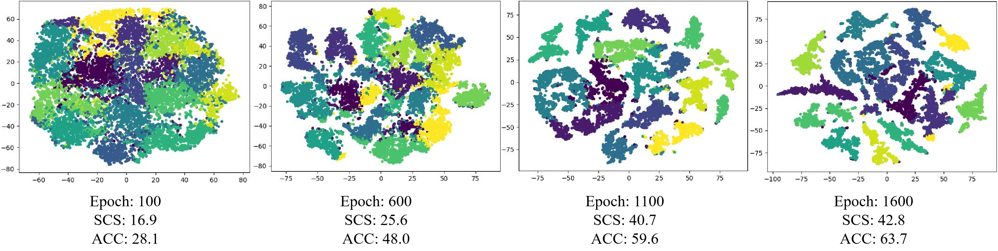
Figure 6: Visualization of clustering feature representations distribution for GJR on ImageNet-Dog. There are four training periods to show the clustering effect with every Epoch, SCS and ACC. SCS presents Silhouette Coefficient Score [61].

Considered the specificity on fine-gained dataset, we show the visualization distribution for GJR on ImageNet-Dog in Fig. 6. We print the figures every 500 epochs from 100 to 1600. This dataset has 15 categories for dogs, so there are more centers to train and cluster. Compared to pGJR, the much epochs are required to train. However, the steady training process and the increasingly tight clusters symbolize the effectiveness of GJR. Here, we provide evaluative Silhouette Coefficient Score (SCS) [61] which presents the contour of clusters. Both of distributions and SCS demonstrate the effectiveness of clustering centers with training samples aggregation.

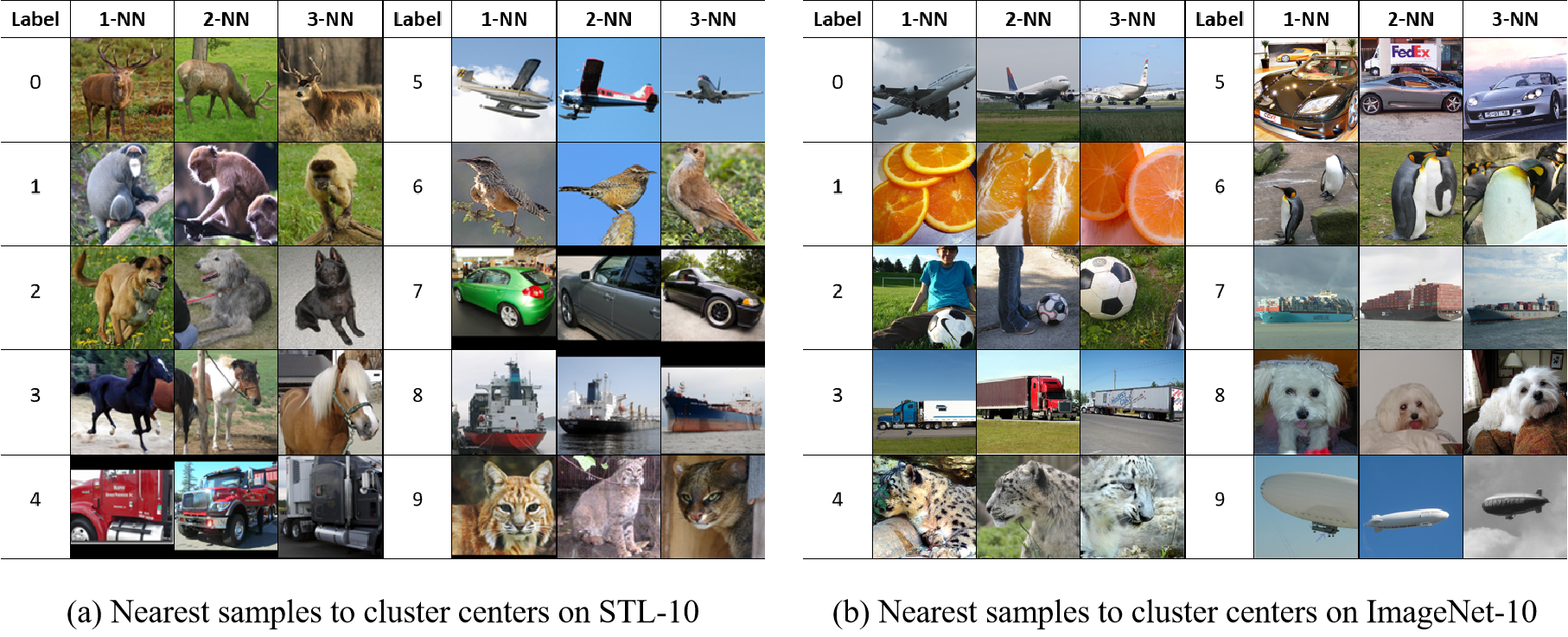
Figure 7: Visualization of semantic clusters on STL10 in Fig. 7(a) and ImageNet-10 in Fig. 7(b). The top three nearest samples called K-NearestNeighbor (KNN) to the cluster centers are shown with 1-NN, 2-NN and 3-NN.

Finally, we analyze semantic clusters through visualization of K-NearestNeighbor (KNN) and we set $k=3$. Fig. 7 shows the top three nearest samples of the cluster centers which we find by calculating the Euclidean distance between the samples and their respective cluster centers. It proved that the nearest samples exactly match the human annotations and gather in their discriminative regions with the cluster centers. For example, the cluster with label ‘0’ captures the ‘deer’ class on STL-10, and its most discriminative regions capture the planes at different locations. Moreover, the cluster with label ‘4’ captures the ‘leopard’ class on ImageNet-10 where the 1-NN and 2-NN samples have the same motion and perspective with just little difference in shade of color and background.

VI Conclusion

In this paper, we propose a new perspective on image clustering jigsaw feature representation (GJR) and pretrain-based visual extractor. Specifically, we expend our previous work which preliminary makes attempt on the grid feature with jigsaw strategy. We systematically expound the motivation and design to verify from pixel to feature in discrepancy against human and computer. Moreover, we propose a new pattern to use the pretrained model CLIP as feature extractor can speed up the convergence of clustering. Further, we innovate pretrain-based Grid Jigsaw Representation (pGJR) to fusion our GJR with CLIP to improve clustering performance. The experiment results show our methods’ capability on visual representation learning and training efficiency for unsupervised image clustering. Meanwhile, we compare the GJR and pGJR especially on fine-grained dataset to provide suggestion for situations in which to use the pretrained model.

References

- [1] J. Hou, H. Gao, and X. Li, “Feature combination via clustering,” IEEE Transactions on Neural Networks and Learning Systems, vol. 29, no. 4, pp. 896–907, 2017.
- [2] Q. Ji, Y. Sun, J. Gao, Y. Hu, and B. Yin, “A decoder-free variational deep embedding for unsupervised clustering,” IEEE Transactions on Neural Networks and Learning Systems, vol. 33, no. 10, pp. 5681–5693, 2021.
- [3] J. Yin, H. Wu, and S. Sun, “Effective sample pairs based contrastive learning for clustering,” Information Fusion, vol. 99, p. 101899, 2023.
- [4] T. Chu, S. Tong, T. Ding, X. Dai, B. D. Haeffele, R. Vidal, and Y. Ma, “Image clustering via the principle of rate reduction in the age of pretrained models,” arXiv preprint arXiv:2306.05272, 2023.
- [5] Q. Qian, “Stable cluster discrimination for deep clustering,” in Proceedings of the IEEE/CVF International Conference on Computer Vision, 2023, pp. 16 645–16 654.
- [6] K. He, X. Zhang, S. Ren, and J. Sun, “Deep residual learning for image recognition,” in Proceedings of the IEEE conference on computer vision and pattern recognition, 2016, pp. 770–778.
- [7] A. Dosovitskiy, L. Beyer, A. Kolesnikov, D. Weissenborn, X. Zhai, T. Unterthiner, M. Dehghani, M. Minderer, G. Heigold, S. Gelly et al., “An image is worth 16x16 words: Transformers for image recognition at scale,” ICLR, 2020.
- [8] M. Noroozi and P. Favaro, “Unsupervised learning of visual representations by solving jigsaw puzzles,” in European conference on computer vision. Springer, 2016, pp. 69–84.
- [9] D. Kim, D. Cho, D. Yoo, and I. S. Kweon, “Learning image representations by completing damaged jigsaw puzzles,” in 2018 IEEE Winter Conference on Applications of Computer Vision (WACV). IEEE, 2018, pp. 793–802.
- [10] P. Chen, S. Liu, and J. Jia, “Jigsaw clustering for unsupervised visual representation learning,” in Proceedings of the IEEE/CVF conference on computer vision and pattern recognition, 2021, pp. 11 526–11 535.
- [11] Z. Song, Z. Hu, and R. Hong, “Grid feature jigsaw for self-supervised image clustering,” in 2023 International Joint Conference on Neural Networks (IJCNN). IEEE, 2023, pp. 1–7.
- [12] A. Radford, J. W. Kim, C. Hallacy, A. Ramesh, G. Goh, S. Agarwal, G. Sastry, A. Askell, P. Mishkin, J. Clark et al., “Learning transferable visual models from natural language supervision,” in International conference on machine learning. PMLR, 2021, pp. 8748–8763.
- [13] J. Chang, L. Wang, G. Meng, S. Xiang, and C. Pan, “Deep adaptive image clustering,” in Proceedings of the IEEE international conference on computer vision, 2017, pp. 5879–5887.
- [14] J. Wu, K. Long, F. Wang, C. Qian, C. Li, Z. Lin, and H. Zha, “Deep comprehensive correlation mining for image clustering,” in Proceedings of the IEEE/CVF international conference on computer vision, 2019, pp. 8150–8159.
- [15] A. Y. Ng, M. I. Jordan, and Y. Weiss, “On spectral clustering: Analysis and an algorithm,” in NeurIPS, 2002, pp. 849–856.
- [16] U. Shaham, K. Stanton, H. Li, B. Nadler, R. Basri, and Y. Kluger, “Spectralnet: Spectral clustering using deep neural networks,” ICLR, 2018.
- [17] F. M. Bianchi, D. Grattarola, and C. Alippi, “Spectral clustering with graph neural networks for graph pooling,” in ICML, 2020, pp. 874–883.
- [18] Z.-Q. Wang and D. Wang, “Combining spectral and spatial features for deep learning based blind speaker separation,” TASLP, vol. 27, no. 2, pp. 457–468, 2018.
- [19] Z. Wu, Y. Xiong, S. X. Yu, and D. Lin, “Unsupervised feature learning via non-parametric instance discrimination,” in Proceedings of the IEEE conference on computer vision and pattern recognition, 2018, pp. 3733–3742.
- [20] X. Yang, C. Deng, F. Zheng, J. Yan, and W. Liu, “Deep spectral clustering using dual autoencoder network,” in CVPR, 2019, pp. 4066–4075.
- [21] Y. Tao, K. Takagi, and K. Nakata, “Clustering-friendly representation learning via instance discrimination and feature decorrelation,” arXiv preprint arXiv:2106.00131, 2021.
- [22] C. Xu, R. Lin, J. Cai, and S. Wang, “Deep image clustering by fusing contrastive learning and neighbor relation mining,” Knowledge-Based Systems, vol. 238, p. 107967, 2022.
- [23] Z. Li, Y. Chen, Y. LeCun, and F. T. Sommer, “Neural manifold clustering and embedding,” arXiv preprint arXiv:2201.10000, 2022.
- [24] T. Chen, S. Kornblith, M. Norouzi, and G. Hinton, “A simple framework for contrastive learning of visual representations,” in International conference on machine learning. PMLR, 2020, pp. 1597–1607.
- [25] J.-B. Grill, F. Strub, F. Altché, C. Tallec, P. Richemond, E. Buchatskaya, C. Doersch, B. Avila Pires, Z. Guo, M. Gheshlaghi Azar et al., “Bootstrap your own latent-a new approach to self-supervised learning,” Advances in neural information processing systems, vol. 33, pp. 21 271–21 284, 2020.
- [26] J. R. Regatti, A. A. Deshmukh, E. Manavoglu, and U. Dogan, “Consensus clustering with unsupervised representation learning,” in IJCNN. IEEE, 2021, pp. 1–9.
- [27] C. Niu, H. Shan, and G. Wang, “Spice: Semantic pseudo-labeling for image clustering,” IEEE Transactions on Image Processing, vol. 31, pp. 7264–7278, 2022.
- [28] T. W. Tsai, C. Li, and J. Zhu, “Mice: Mixture of contrastive experts for unsupervised image clustering,” in International conference on learning representations, 2020.
- [29] K. Do, T. Tran, and S. Venkatesh, “Clustering by maximizing mutual information across views,” in Proceedings of the IEEE/CVF international conference on computer vision, 2021, pp. 9928–9938.
- [30] F. M. Carlucci, A. D’Innocente, S. Bucci, B. Caputo, and T. Tommasi, “Domain generalization by solving jigsaw puzzles,” in Proceedings of the IEEE/CVF Conference on Computer Vision and Pattern Recognition, 2019, pp. 2229–2238.
- [31] L. Dery, R. Mengistu, and O. Awe, “Neural combinatorial optimization for solving jigsaw puzzles: A step towards unsupervised pre-training,” 2017.
- [32] M.-M. Paumard, D. Picard, and H. Tabia, “Jigsaw puzzle solving using local feature co-occurrences in deep neural networks,” in ICIP, 2018, pp. 1018–1022.
- [33] M. Abdolahnejad and P. X. Liu, “Face images as jigsaw puzzles: Compositional perception of human faces for machines using generative adversarial networks,” arXiv preprint arXiv:2103.06331, 2021.
- [34] X. Chen and K. He, “Exploring simple siamese representation learning,” in Proceedings of the IEEE/CVF conference on computer vision and pattern recognition, 2021, pp. 15 750–15 758.
- [35] J. Zbontar, L. Jing, I. Misra, Y. LeCun, and S. Deny, “Barlow twins: Self-supervised learning via redundancy reduction,” in International Conference on Machine Learning. PMLR, 2021, pp. 12 310–12 320.
- [36] A. Bardes, J. Ponce, and Y. LeCun, “Vicreg: Variance-invariance-covariance regularization for self-supervised learning,” in 10th International Conference on Learning Representations, ICLR 2022, 2022.
- [37] X. Chen, M. Ding, X. Wang, Y. Xin, S. Mo, Y. Wang, S. Han, P. Luo, G. Zeng, and J. Wang, “Context autoencoder for self-supervised representation learning,” International Journal of Computer Vision, pp. 1–16, 2023.
- [38] K. He, G. Gkioxari, P. Dollár, and R. Girshick, “Mask r-cnn,” in CVPR, 2017, pp. 2961–2969.
- [39] S. Ren, K. He, R. Girshick, and J. Sun, “Faster r-cnn: Towards real-time object detection with region proposal networks,” NeurIPS, vol. 28, pp. 91–99, 2015.
- [40] H. Jiang, I. Misra, M. Rohrbach, E. Learned-Miller, and X. Chen, “In defense of grid features for visual question answering,” in CVPR, 2020, pp. 10 267–10 276.
- [41] J. Devlin, M.-W. Chang, K. Lee, and K. Toutanova, “Bert: Pre-training of deep bidirectional transformers for language understanding,” arXiv preprint arXiv:1810.04805, 2018.
- [42] N. Parmar, A. Vaswani, J. Uszkoreit, L. Kaiser, N. Shazeer, A. Ku, and D. Tran, “Image transformer,” in ICML, 2018, pp. 4055–4064.
- [43] D. Qi, L. Su, J. Song, E. Cui, T. Bharti, and A. Sacheti, “Imagebert: Cross-modal pre-training with large-scale weak-supervised image-text data,” arXiv preprint arXiv:2001.07966, 2020.
- [44] Z. Huang, Z. Zeng, B. Liu, D. Fu, and J. Fu, “Pixel-bert: Aligning image pixels with text by deep multi-modal transformers,” arXiv preprint arXiv:2004.00849, 2020.
- [45] K. He, X. Chen, S. Xie, Y. Li, P. Dollár, and R. Girshick, “Masked autoencoders are scalable vision learners,” arXiv preprint arXiv:2111.06377, 2021.
- [46] L. Wang, S. Ding, Y. Wang, and L. Ding, “A robust spectral clustering algorithm based on grid-partition and decision-graph,” IJMLC, vol. 12, no. 5, pp. 1243–1254, 2021.
- [47] K. He, X. Chen, S. Xie, Y. Li, P. Dollár, and R. Girshick, “Masked autoencoders are scalable vision learners,” in Proceedings of the IEEE/CVF conference on computer vision and pattern recognition, 2022, pp. 16 000–16 009.
- [48] A. Krizhevsky, G. Hinton et al., “Learning multiple layers of features from tiny images,” 2009.
- [49] A. Coates, A. Ng, and H. Lee, “An analysis of single-layer networks in unsupervised feature learning,” in Proceedings of the fourteenth international conference on artificial intelligence and statistics. JMLR Workshop and Conference Proceedings, 2011, pp. 215–223.
- [50] J. Deng, W. Dong, R. Socher, L.-J. Li, K. Li, and L. Fei-Fei, “Imagenet: A large-scale hierarchical image database,” in 2009 IEEE conference on computer vision and pattern recognition. Ieee, 2009, pp. 248–255.
- [51] J. Xie, R. Girshick, and A. Farhadi, “Unsupervised deep embedding for clustering analysis,” in International conference on machine learning. PMLR, 2016, pp. 478–487.
- [52] X. Ji, J. F. Henriques, and A. Vedaldi, “Invariant information clustering for unsupervised image classification and segmentation,” in Proceedings of the IEEE/CVF international conference on computer vision, 2019, pp. 9865–9874.
- [53] J. Huang, S. Gong, and X. Zhu, “Deep semantic clustering by partition confidence maximisation,” in Proceedings of the IEEE/CVF conference on computer vision and pattern recognition, 2020, pp. 8849–8858.
- [54] H. Zhong, C. Chen, Z. Jin, and X.-S. Hua, “Deep robust clustering by contrastive learning,” arXiv preprint arXiv:2008.03030, 2020.
- [55] W. Van Gansbeke, S. Vandenhende, S. Georgoulis, M. Proesmans, and L. Van Gool, “Scan: Learning to classify images without labels,” in European conference on computer vision. Springer, 2020, pp. 268–285.
- [56] F. Ntelemis, Y. Jin, and S. A. Thomas, “Information maximization clustering via multi-view self-labelling,” Knowledge-Based Systems, vol. 250, p. 109042, 2022.
- [57] Y. Li, M. Yang, D. Peng, T. Li, J. Huang, and X. Peng, “Twin contrastive learning for online clustering,” International Journal of Computer Vision, vol. 130, no. 9, pp. 2205–2221, 2022.
- [58] J. Li, P. Zhou, C. Xiong, and S. Hoi, “Prototypical contrastive learning of unsupervised representations,” in International Conference on Learning Representations, 2020.
- [59] K. Simonyan and A. Zisserman, “Very deep convolutional networks for large-scale image recognition,” arXiv preprint arXiv:1409.1556, 2014.
- [60] G. Huang, Z. Liu, L. Van Der Maaten, and K. Q. Weinberger, “Densely connected convolutional networks,” in Proceedings of the IEEE conference on computer vision and pattern recognition, 2017, pp. 4700–4708.
- [61] S. Aranganayagi and K. Thangavel, “Clustering categorical data using silhouette coefficient as a relocating measure,” in International conference on computational intelligence and multimedia applications (ICCIMA 2007), vol. 2. IEEE, 2007, pp. 13–17.