Asymmetric Geometry of Total Grassmannians

Abstract

Metrics in Grassmannians, or distances between subspaces of same dimension, have many applications. However, usual extensions to the Total Grassmannian of subspaces of different dimensions lack useful properties or give little information. Dimensional asymmetries call for the use of asymmetric metrics, which arise naturally in this space. Their geometry reflects containment relations of subspaces, and minimal geodesics link subspaces of distinct dimensions. In particular, the Fubini-Study metric extends as an asymmetric angle with useful properties, that can be computed in arbitrary bases or via Grassmann algebra. It has a nice geometric interpretation, as does its sine, an asymmetric Binet-Cauchy metric.

Keywords: Grassmannian, Grassmann manifold, asymmetric metric, distance between subspaces, angle between subspaces, Fubini-Study.

MSC 2020: Primary 14M15; Secondary 15A75, 51K99

1 Introduction

Various metrics in Grassmannians, sets of subspaces of a given dimension [1, 2, 3, 4], are used to measure the separation of such subspaces [5, 6, 7, 8]: geodesic, gap, projection Frobenius, Fubini-Study, etc. They are important in geometry, linear algebra, functional analysis, and applications where subspaces are used to represent data: wireless communication [9, 10, 11], coding theory [12, 13, 14], machine learning [15, 16, 17], computer vision [18, 19, 20], etc.

Some problems [21, 22, 23, 24, 25, 26, 27, 28, 29] require the Total Grassmannian of subspaces of different dimensions, but distances used in it have various shortcomings. Distances [22, 23, 24] from the smaller subspace to its projection on the larger one fail the triangle inequality (e.g. take two lines and their plane). When dimensions differ the gap [8] is always 1, not giving any information, and the symmetric distance [30, 29] is at least $1$. It can be best to have $d(V,W)=0$ if $V\subset W$ [25, 26], which usual metrics do not allow. The containment gap [8, 27, 28] satisfies this, but gives little information (only the largest principal angle). Other metrics in [21] have similar issues.

Any (symmetric) metric in the Total Grassmannian is bound to have problems, as subspaces of different dimensions have inherently asymmetric relations (e.g. a plane contains lines, not vice versa; areas projected on a line vanish, lengths projected on a plane tend not to). And though its usual topology, as a disjoint union of Grassmannians, arises naturally in some models, it is sometimes inadequate, separating a plane from its lines, for example. As it is disconnected, processes with dimension changes (e.g. data compression) are discontinuous. A better topology should reflect the idea that a small region around a line contains no planes, but near a plane we have lines; and a line can move continuously into a given plane (or the plane move to contain the line), not vice versa.

The symmetry $d(x,y)=d(y,x)$ of metrics has long been recognized as an overly restrictive simplifying assumption, as often the path, time or cost to go from $x$ to $y$ is not the same as from $y$ to $x$: one-way streets, rush-hour traffic, uphill or downhill, etc. The separation condition $d(x,y)=0\Leftrightarrow x=y$ is also too strong sometimes (e.g. for subspaces). The triangle inequality, $d(x,z)\leq d(x,y)+d(y,z)$, is what matters most: without it open balls do not generate a topology; and if $d(x,z)$ measures an optimal way to go from $x$ to $z$, it can not be worse than going through $y$.

Asymmetric metrics or quasi-metrics [31, 32, 33, 34, 35] occur in topology [36, 37, 38], Finsler geometry [39], category theory [40, 41], computer science [42, 43, 44], graph theory [45], biology [46], etc. Richer than metrics, they carry data in $d(x,y)$ and $d(y,x)$, and distances to or from a point split usual concepts into backward and forward ones, a common duality in asymmetric structures [47, 48]. A weaker separation condition lets them generalize partial orders $\leq$, with $d(x,y)$ measuring the failure of $x\leq y$. They induce two non-Hausdorff topologies, linked to $\leq$ and $\geq$, which complement each other and combine into a metric topology. Many metric results have asymmetric versions, while some asymmetric ones have only trivial metric analogues [49, 50, 51, 52, 53, 48, 54]. The containment gap [8, 27, 28] is an example in the Total Grassmannian, but its asymmetry has not been explored.

As we show, Grassmannian metrics extend naturally as asymmetric metrics in the Total Grassmannian. These are similar to the original metrics, and should be just as practical. They measure how far a subspace is from being contained in another (as far as possible, if the first one is larger), and give topologies reflecting the relations $\subset$, $\supset$, and $=$ (the usual topology). We describe their geometry, obtain minimal geodesics connecting subspaces of any dimensions, and determine when geodesics are segments and the triangle inequality attains equality.

Special attention is given to the Fubini-Study metric, used with complex spaces in wireless communication [12, 10, 11, 24] and quantum theory [55]. It extends as an asymmetric angle [56] whose cosine (squared, in the complex case) measures volume contraction in orthogonal projections. Links to Grassmann and Clifford algebras [57, 58] give useful properties [59] and easy ways to compute it. It has led to complex Pythagorean theorems [60] with interesting implications for quantum theory [61]. Its sine, an asymmetric Binet-Cauchy metric, also has a nice geometric interpretation.

Section 2 sets up notation and reviews concepts. Section 3 obtains asymmetric metrics in the Total Grassmannian. Section 4 describes their geometries. Section 5 studies the asymmetric Fubini-Study and Binet-Cauchy metrics. Section 6 closes with some remarks. Appendix A reviews Grassmann exterior algebra. Appendix B reviews and organizes the main Grassmannian metrics.

2 Preliminaries

We will use $\mathds{F}^{n}$, for $\mathds{F}=\mathds{R}$ or $\mathds{C}$, with inner product $\langle\cdot,\cdot\rangle$ (Hermitian product if $\mathds{F}=\mathds{C}$, in which case its real part $\operatorname{Re}\langle\cdot,\cdot\rangle$ is an inner product in the underlying real space $\mathds{R}^{2n}$). A $p$-dimensional subspace is a $p$-subspace, or line if $p=1$. For a subspace $V$, $G_{p}(V)=\{p$-subspaces of $V\}$ is a Grassmannian, and $G(V)=\{$subspaces of $V\}$ is a Total Grassmannian. We also write $G_{p}^{n}=G_{p}(\mathds{F}^{n})$, $G^{n}=G(\mathds{F}^{n})$, and $P_{V}:\mathds{F}^{n}\rightarrow V$ is an orthogonal projection. For nonzero $v,w\in\mathds{F}^{n}$ let $\theta_{v,w}=\cos^{-1}\frac{\operatorname{Re}\langle v,w\rangle}{\|v\|\|w\|}$ and $\theta_{v,0}=\frac{\pi}{2}$, and for any $v\in\mathds{F}^{n}$ let $\theta_{0,v}=0$ (note the asymmetry $\theta_{v,0}\neq\theta_{0,v}$ if $v\neq 0$).

2.1 Asymmetric metrics

We define asymmetric metrics as follows [34, 36, 51, 35, 52, 54, 53]. Some authors call them quasi-metrics, a term often used for a closely related concept [31, 32, 33, 49, 50, 48] with a $T_{1}$ separation condition ($d(x,y)=0\Leftrightarrow x=y$).

Definition 2.1.

An asymmetric metric is a function $d:M\times M\rightarrow[0,\infty]$ on a set $M$ satisfying, for all $x,y,z\in M$:

1. $d(x,y)=d(y,x)=0\Leftrightarrow x=y$  ($T_{0}$ separation condition).

2. $d(x,z)\leq d(x,y)+d(y,z)$  (Oriented triangle inequality).

The $T_{0}$ condition lets $d$ induce a partial order by $x\leq y\Leftrightarrow d(x,y)=0$, and any partial order can be represented by some $d$.

Any permutation-invariant monotone norm $\|\cdot\|$ in $\mathds{R}^{2}$ symmetrizes $d$ (with some loss of information) into a metric $\rho(x,y)=\|(d(x,y),d(y,x))\|$. The max-symmetrized metric is $\hat{d}(x,y)=\max\{d(x,y),d(y,x)\}$.

Backward, forward and symmetric topologies $\tau^{-}$, $\tau^{+}$, $\tau$ are generated by backward balls $B^{-}_{r}(x)=\{y\in M:d(y,x)<r\}$, forward balls $B^{+}_{r}(x)=\{y\in M:d(x,y)<r\}$, and symmetric balls $B_{r}(x)=B^{+}_{r}(x)\cap B^{-}_{r}(x)$. In general, $\tau^{\pm}$ are only $T_{0}$, but well behaved, complementing each other and combining into $\tau$, which is the metric topology of $\hat{d}$, hence Hausdorff.

Analysis in $M$ requires some care. With $T_{0}$, limits are not unique. By ii, $d(x_{k},y)-d(x,y)\leq d(x_{k},x)$ and $d(x,y_{k})-d(x,y)\leq d(y,y_{k})$, so in $\tau^{-}$ we have that $d(x,y)$ is upper semicontinuous in $x$ and lower semicontinuous in $y$, in $\tau^{+}$ it is the opposite, and in $\tau$ it is continuous. A sequence $x_{k}$ is left (resp. right) K-Cauchy if given $\epsilon>0$ there is $n\in\mathds{N}$ such that $d(x_{k},x_{l})<\epsilon$ (resp. $d(x_{l},x_{k})<\epsilon$) whenever $n\leq k\leq l$. If any such sequence has $\hat{d}(x_{k},x)\rightarrow 0$ for some $x\in M$ then $(M,d)$ is left (resp. right) Smyth complete. It is Smyth bicomplete if both.

A map $f:(M_{1},d_{1})\rightarrow(M_{2},d_{2})$ of asymmetric metric spaces is an isometry if $d_{1}(x,y)=d_{2}(f(x),f(y))$ for all $x,y\in M_{1}$, an anti-isometry if $d_{1}(x,y)=d_{2}(f(y),f(x))$. A bijective isometry gives homeomorphisms $\tau_{1}\simeq\tau_{2}$ and $\tau_{1}^{\pm}\simeq\tau_{2}^{\pm}$ of the corresponding topologies of $M_{1}$ and $M_{2}$. A bijective anti-isometry gives $\tau_{1}\simeq\tau_{2}$ and $\tau_{1}^{\pm}\simeq\tau_{2}^{\mp}$ (so, switching backward and forward topologies). We write $\operatorname{Isom}(M)$ for the group of isometries of $M$, and $\operatorname{Transf}(M)$ for that of its isometries and anti-isometries.

A curve in $M$ (for $\tau$ or $\tau^{\pm}$) is a continuous $\varphi:I\rightarrow M$, for an interval $I\subset\mathds{R}$. If $I=[a,b]$, it is a path from $\varphi(a)$ to $\varphi(b)$. Being coarser, $\tau^{\pm}$ have more curves than $\tau$: in $\tau^{-}$, $\varphi$ is continuous at $t$ if $\lim_{s\rightarrow t}d(\varphi(s),\varphi(t))=0$; in $\tau^{+}$, if $\lim_{s\rightarrow t}d(\varphi(t),\varphi(s))=0$; and $\tau$ needs both. A curve is rectifiable if it has finite length $\ell_{\varphi}=\sup\sum_{i=1}^{N-1}d(\varphi(t_{i}),\varphi(t_{i+1}))$, with the $\sup$ over all finite sequences $t_{1}<\cdots<t_{N}$ in $I$. It is null if $\ell_{\varphi}=0$. The reversed curve $\varphi(-t)$ can be non-rectifiable or have a different length. If $f$ is an anti-isometry, $f\circ\varphi$ and $\varphi(-t)$ have the same length. In $\tau^{\pm}$, the length of a restricted curve $\varphi\lvert_{[a,t]}$ can vary discontinuously with $t$.

The infimum of lengths of paths from $x$ to $y$ gives a (topology dependent) intrinsic asymmetric metric $D(x,y)$, and $d$ is intrinsic if $D=d$. A path $\varphi$ from $x$ to $y$ is a minimal geodesic if $\ell_{\varphi}=D(x,y)$, and a segment if $\ell_{\varphi}=d(x,y)$. $M$ is a geodesic space if any two points are linked by a minimal geodesic. If $d(x,z)=d(x,y)+d(y,z)$ then $y$ is a between-point from $x$ to $z$ (is between them, if both ways). This holds for $y$ in a segment. $M$ is convex if any distinct $x,z\in M$ have a between-point $y\neq x,z$.

Example 2.2.

The asymmetric metric $d(x,y)=\max\{0,x-y\}$ in $\mathds{R}$ induces the usual order, and measures how much $x\leq y$ fails. The metric $\hat{d}(x,y)=|x-y|$ measures the failure in $x=y$, and loses information about which is bigger. While $\tau$ is the usual topology, $\tau^{-}$ is the upper semicontinuous one, and $\tau^{+}$ the lower one. The anti-isometry $f:\mathds{R}\rightarrow\mathds{R}$, $f(x)=-x$, gives a self-homeomorphism of $\tau$ (the usual reflection symmetry of $\mathds{R}$), and switches the asymmetric topologies $\tau^{+}$ and $\tau^{-}$ (which, in a sense, split the symmetry of $\tau$). As $x_{k}=k$ (resp. $x_{k}=-k$) is left (resp. right) K-Cauchy, $(\mathds{R},d)$ is neither left nor right Smyth complete. But $(-\infty,0]$ is left Smyth complete, as any left K-Cauchy sequence in it is Cauchy for $\hat{d}$ (any sequence has $d(x_{k},0)=0$, which explains why Smyth completeness uses $\hat{d}$). Likewise, $[0,\infty)$ is right Smyth complete.

The next example is a toy model for some features we will encounter in the Total Grassmannian.

Example 2.3.

In $M=\{0,1,\ldots,n\}$, an asymmetric metric is given by $d(p,q)=0$ if $p\leq q$, $1$ otherwise. It is Smith bicomplete, as any left or right K-Cauchy sequence eventually becomes constant. Open sets in $M^{-}=(M,\tau^{-})$ are $\{0,1,\ldots,p\}$ for $p\in M$, in $M^{+}=(M,\tau^{+})$ they are $\{p,p+1,\ldots,n\}$, and $\tau$ is discrete. The anti-isometry $f:M\rightarrow M$, $f(p)=n-p$, switches $M^{-}$ and $M^{+}$. In $M^{-}$, $\varphi(t)=\begin{cases}p&\text{for }t\in[0,1),\\ q&\text{for }t\in[1,2],\end{cases}$ is a null minimal geodesic from $p$ to $q>p$, and $\varphi(-t)$ is a minimal geodesic from $q$ to $p$, of length $1$. In $M^{+}$ we have the same with $[0,1]$ and $(1,2]$. So $M^{\pm}$ are geodesic spaces with $d$ intrinsic. We can also construct minimal geodesics from $p$ to $q$ passing through $p,p+1,\ldots,q$, whose reversed paths are not minimal geodesics. For $r<p<q<s$, we can construct minimal geodesics from $q$ to $p$ passing through $q,q+1,\ldots,s,r,r+1,\ldots,p$.

2.2 Principal angles

The principal angles [62, 7, 5] of $V\in G_{p}^{n}$ and $W\in G_{q}^{n}$, with $m=\min\{p,q\}\neq 0$, are $0\leq\theta_{1}\leq\cdots\leq\theta_{m}\leq\frac{\pi}{2}$ if there are orthonormal bases $(e_{1},\ldots,e_{p})$ of $V$ and $(f_{1},\ldots,f_{q})$ of $W$ with $e_{i}\perp f_{j}$ for $i\neq j$, and $\theta_{e_{i},f_{i}}=\theta_{i}$ for $i\leq m$. Such principal bases are formed by principal vectors, orthonormal eigenvectors of $P^{*}P$ and $PP^{*}$, where $P:V\rightarrow W$ is the orthogonal projection and $P^{*}$ its adjoint. The eigenvalues of $P^{*}P$ if $p\leq q$, or $PP^{*}$ if $p>q$, are the $\cos^{2}\theta_{i}$’s, and $\theta_{i}=\theta_{e_{i},P_{W}e_{i}}=\min\{\theta_{v,P_{W}v}:0\neq v\in V,v\perp e_{j}\ \forall j<i\}=\min\limits_{U\in G_{i}(V)}\max\limits_{v\in U}\theta_{v,P_{W}v}=\max\limits_{U\in G_{p+1-i}(V)}\min\limits_{0\neq v\in U}\theta_{v,P_{W}v}$. The number of null $\theta_{i}$’s is $\dim(V\cap W)$.

Proposition 2.4.

Let $V\in G_{p}^{n}$, $W\in G_{q}^{n}$, $W^{\prime}\in G_{r}(W)$, $m=\min\{p,q\}\neq 0$, $m^{\prime}=\min\{p,r\}\neq 0$, $\theta_{1}\leq\cdots\leq\theta_{m}$ be the principal angles of $V$ and $W$, $\theta_{1}^{\prime}\leq\cdots\leq\theta_{m^{\prime}}^{\prime}$ be those of $V$ and $W^{\prime}$, and set $\theta_{i}=\frac{\pi}{2}$ for $i>m$. Then $\theta_{i}\leq\theta_{i}^{\prime}\leq\theta_{i+q-r}$ for all $1\leq i\leq m^{\prime}$. Also:

1. $\theta_{i}^{\prime}=\theta_{i}$ for all $1\leq i\leq m^{\prime}\Leftrightarrow W^{\prime}=\operatorname{span}\{f_{1},\ldots,f_{r}\}$ for a principal basis $(f_{1},\ldots,f_{q})$ of $W$ w.r.t. $V$.

2. $\theta_{i}^{\prime}=\theta_{i+q-r}$ for all $1\leq i\leq m^{\prime}\Leftrightarrow W^{\prime}=\operatorname{span}\{f_{1+q-r},\ldots,f_{q}\}$ for a principal basis $(f_{1},\ldots,f_{q})$ of $W$ w.r.t. $V$.

Proof.

$\theta_{i}^{\prime}=\min\limits_{U\in G_{i}(V)}\max\limits_{v\in U}\theta_{v,P_{W^{\prime}}v}\geq\min\limits_{U\in G_{i}(V)}\max\limits_{v\in U}\theta_{v,P_{W}v}=\theta_{i}$, and also $\theta_{i}^{\prime}=\max\limits_{U\in G_{r+1-i}(W^{\prime})}\min\limits_{0\neq w\in U}\theta_{w,P_{V}w}\leq\max\limits_{U\in G_{r+1-i}(W)}\min\limits_{0\neq w\in U}\theta_{w,P_{V}w}=\theta_{i+q-r}$ if $i+q-r\leq m$. Let $(e_{1}^{\prime},\ldots,e_{p}^{\prime})$ and $(f_{1}^{\prime},\ldots,f_{r}^{\prime})$ be principal bases of $V$ and $W^{\prime}$. (i) If $\theta_{e_{i}^{\prime},f_{i}^{\prime}}=\theta_{i}^{\prime}=\theta_{i}\ \forall i\leq m^{\prime}$ then $(e_{1}^{\prime},\ldots,e^{\prime}_{m^{\prime}})$ and $(f_{1}^{\prime},\ldots,f_{r}^{\prime})$ extend to principal bases of $V$ and $W$. (ii) Let $j(i)=i+q-r$ and suppose $\theta_{i}^{\prime}=\theta_{j(i)}$ for $i\leq m^{\prime}$. If $q\leq p$ then $m^{\prime}=r$, $j(m^{\prime})=q=m$ and $(\theta_{1}^{\prime},\ldots,\theta_{m^{\prime}}^{\prime})=(\theta_{1+q-r},\ldots,\theta_{m})$, so $f_{1}^{\prime},\ldots,f_{r}^{\prime}$ can be used as last vectors of a principal basis of $W$ w.r.t. $V$. If $q>p$, the last $q-p$ vectors of such basis are orthogonal to $V$, and $f_{1}^{\prime},\ldots,f_{r}^{\prime}$ can be used as some of them if $q\geq p+r$, as $j(i)>p=m$ and $\theta_{i}^{\prime}=\frac{\pi}{2}$ for $i\leq m^{\prime}$, and $f_{i}^{\prime}\perp V$ for $i>m^{\prime}$. If $p<q<p+r$ then $1\leq p+r-q\leq m^{\prime}$ and $j(p+r-q)=m$, so $(\theta_{1}^{\prime},\ldots,\theta_{p+r-q}^{\prime})=(\theta_{1+q-r},\ldots,\theta_{m})$ and $\theta_{i}^{\prime}=\frac{\pi}{2}$ for $p+r-q<i\leq m^{\prime}$, and again we obtain the result. ∎

2.3 Grassmannians

The Grassmannian $G_{p}^{n}$ is a connected compact manifold of dimension $p(n-p)$ [1, 2, 3, 4]. See Appendix B for a classification of its metrics. Curve lengths coincide for $l^{2}$ and $\wedge$ metrics, which converge asymptotically for small $\theta_{i}$’s [6, p. 337]. For them, any minimal geodesic from $V$ to $W$ is given by $\varphi(t)=\operatorname{span}\{v_{1}(t),\ldots,v_{p}(t)\}$, where $t\in[0,1]$ and $v_{i}(t)=\cos(t\theta_{i})e_{i}+\sin(t\theta_{i})\frac{f_{i}-P_{V}f_{i}}{\|f_{i}-P_{V}f_{i}\|}$ ($=e_{i}$ if $\theta_{i}=0$) for principal bases $(e_{1},\ldots,e_{p})$ and $(f_{1},\ldots,f_{p})$ and principal angles $\theta_{1}\leq\cdots\leq\theta_{p}$, so that the $e_{i}$’s rotate at constant speeds towards the $f_{i}$’s. Its length is the geodesic metric $d_{g}(V,W)=\sqrt{\sum_{i=1}^{p}\theta_{i}^{2}}$. If $X\subset(V+W)^{\perp}$, $\varphi(t)\oplus X$ is a minimal geodesic from $V\oplus X$ to $W\oplus X$, of same length. For $d_{g}$, $U$ is between $V$ and $W\Leftrightarrow U$ is in a minimal geodesic from $V$ to $W$.

The Total Grassmannian $G^{n}=\bigcup_{p=0}^{n}G_{p}^{n}$ usually has the disjoint union topology (we will obtain other topologies). Let $V\in G_{p}^{n}$, $W\in G_{q}^{n}$, $m=\min\{p,q\}\neq 0$, $\theta_{1}\leq\cdots\leq\theta_{m}$ be their principal angles, and $(e_{1},\ldots,e_{p})$ be a principal basis of $V$ w.r.t. $W$. We have the following distances between $V$ and $W$ (using $\|\cdot\|_{F}$ and $\|\cdot\|$ for Frobenius and operator norms):

• The Fubini-Study metric extends via Plücker embedding (see Section B.1) as $\hat{d}_{FS}=\cos^{-1}(\prod_{i=1}^{p}\cos\theta_{i})$ if $p=q$, or $\frac{\pi}{2}$ if $p\neq q$.

• $d_{pF}=\frac{1}{\sqrt{2}}\|P_{V}-P_{W}\|_{F}=\sqrt{\frac{|p-q|}{2}+\sum_{i=1}^{m}\sin^{2}\theta_{i}}$ and the symmetric distance [30, 29] $d_{s}=\sqrt{|p-q|+\sum_{i=1}^{m}\sin^{2}\theta_{i}}$ extend $d_{pF}$ as metrics. The triangle inequality fails for $\check{d}_{pF}=\sqrt{\sum_{i=1}^{m}\sin^{2}\theta_{i}}$ [22, 23], and is unknown for the asymmetric directional distance [29] $\vec{d}(V,W)=\sqrt{\sum_{i=1}^{p}\|e_{i}-P_{W}e_{i}\|^{2}}=\sqrt{\max\{0,p-q\}+\sum_{i=1}^{m}\sin^{2}\theta_{i}}$.

• The containment gap [27, 8, 28] extends $d_{p2}$ as an asymmetric metric $\delta(V,W)=\max_{v\in V,\|v\|=1}\|v-P_{W}v\|=\sin\theta_{p}$ if $p\leq q$, or 1 if $p>q$. The gap [8] is a metric $\hat{\delta}=\max\{\delta(V,W),\delta(W,V)\}=\|P_{V}-P_{W}\|=\sin\theta_{p}$ if $p=q$, or 1 if $p\neq q$.

Lack of a triangle inequality limits the utility of $\check{d}_{pF}$ and (maybe) $\vec{d}$. As $\delta$ and $\hat{\delta}$ use only $\theta_{p}$, they give little information, and $\hat{\delta}$ and $\hat{d}_{FS}$ give none if $p\neq q$. As $d_{pF}$, $d_{s}$, $\hat{\delta}$ and $\hat{d}_{FS}$ never approach $0$ when $p\neq q$, subspaces of distinct dimensions are kept apart, making it harder to detect when one is almost contained in the other [25, 26].

The Infinite Grassmannian $G_{p}^{\infty}=\bigcup_{n}G_{p}^{n}$ of $p$-subspaces in all $\mathds{F}^{n}$’s, and Infinite Total Grassmannian $G^{\infty}=\bigcup_{n}G^{n}=\bigcup_{p}G_{p}^{\infty}$ of all subspaces in all $\mathds{F}^{n}$’s, are defined using the natural inclusion $G_{p}^{n}\subset G_{p}^{n+1}$. In [21], metrics $d_{p}$ in $G_{p}^{\infty}$ are extended to $G^{\infty}$: for $V\in G_{p}^{\infty}$ and $W\in G_{q}^{\infty}$, with $p\leq q$, an ad hoc inclusion of $\theta_{p+1}=\cdots=\theta_{q}=\frac{\pi}{2}$ turns $\min\{d_{p}(V,U):U\in G_{p}(W)\}=\min\{d_{q}(Y,W):Y\in G_{q}^{\infty},Y\supset V\}$ into a metric $d(V,W)=\max\{d_{q}(Y,W):Y\in G_{q}^{\infty},Y\supset V\}$. But the metrics obtained have the same problems as those above.

3 Asymmetric metrics in $G^{\infty}$ and $G^{n}$

We will obtain an asymmetric metric $d:G^{\infty}\times G^{\infty}\rightarrow[0,\infty)$ extending naturally a family of metrics $d_{p}:G_{p}^{\infty}\times G_{p}^{\infty}\rightarrow[0,\infty)$ such that, for $p>0$:

1. $d_{p}(V,W)=f_{p}(\theta_{1},\ldots,\theta_{p})$ for a nondecreasing function $f_{p}$ of the principal angles $\theta_{1}\leq\cdots\leq\theta_{p}$ of $V,W\in G_{p}^{\infty}$;

2. $f_{q}(0,\ldots,0,\theta_{1},\ldots,\theta_{p})=f_{p}(\theta_{1},\ldots,\theta_{p})$ for $q>p$.

All metrics of Appendix B satisfy these conditions.

Lemma 3.1.

$\Delta_{p}=\operatorname{diam}G_{p}^{\infty}=\sup\{d_{p}(V,W):V,W\in G_{p}^{\infty}\}$ is a non-decreasing function of $p$.

Proof.

As $G_{p}^{\infty}$, $p\neq 0$, has orthogonal subspaces, for $p<q$ we have $\Delta_{p}=f_{p}(\frac{\pi}{2},\ldots,\frac{\pi}{2})=f_{q}(0,\ldots,0,\frac{\pi}{2},\ldots,\frac{\pi}{2})\leq f_{q}(\frac{\pi}{2},\ldots,\frac{\pi}{2})=\Delta_{q}$. ∎

Table 1 has $\Delta_{p}$ for the metrics of Appendix B. Note that $\operatorname{diam}G_{p}^{n}$ would decrease for $p>\frac{n}{2}$, as subspaces intersect non-trivially.

Type	Metric	$\Delta_{p}$	Asymmetric metric in $G^{\infty}$ or $G^{n}$
$l^{2}$	$d_{g}$	$\frac{\pi}{2}\sqrt{p}$	$\sqrt{\sum_{i=1}^{p}\theta_{i}^{2}}$ if $p\leq q$, otherwise $\frac{\pi}{2}\sqrt{p}$
	$d_{cF}$	$\sqrt{2p}$	$2\sqrt{\sum_{i=1}^{p}\sin^{2}\frac{\theta_{i}}{2}}$ if $p\leq q$, otherwise $\sqrt{2p}$
	$d_{pF}$	$\sqrt{p}$	$\sqrt{\sum_{i=1}^{p}\sin^{2}\theta_{i}}$ if $p\leq q$, otherwise $\sqrt{p}$
$\wedge$	$d_{FS}$	$\frac{\pi}{2}$	$\cos^{-1}(\prod_{i=1}^{p}\cos\theta_{i})$ if $p\leq q$, otherwise $\frac{\pi}{2}$
	$d_{c\wedge}$	$\sqrt{2}$	$\sqrt{2-2\prod_{i=1}^{p}\cos\theta_{i}}$ if $p\leq q$, otherwise $\sqrt{2}$
	$d_{BC}$	$1$	$\sqrt{1-\prod_{i=1}^{p}\cos^{2}\theta_{i}}$ if $p\leq q$, otherwise $1$
max	$d_{A}$	$\frac{\pi}{2}$	$\theta_{p}$ if $p\leq q$, otherwise $\frac{\pi}{2}$
	$d_{c2}$	$\sqrt{2}$	$2\sin\frac{\theta_{p}}{2}$ if $p\leq q$, otherwise $\sqrt{2}$
	$d_{p2}$	$1$	$\sin\theta_{p}$ if $p\leq q$, otherwise $1$

Table 1: Diameter of $G_{p}^{\infty}$, $p\neq 0$, and asymmetric metrics from $V\in G_{p}^{\infty}$ to $W\in G_{q}^{\infty}$

Definition 3.2.

A projection subspace of $W\in G_{q}^{\infty}$ w.r.t. $V\in G_{p}^{\infty}$ is any $W^{\prime}\in G_{\min\{p,q\}}(W)$ such that $P_{W}(V)\subset W^{\prime}$.

For $p,q\neq 0$, $V$ and $W^{\prime}$ have the same principal angles as $V$ and $W$.

Lemma 3.3.

Let $V,W\in G_{p}^{\infty}$ and $V^{\prime}\in G_{r}(V)$. If $W^{\prime}$ is a projection subspace of $W$ w.r.t. $V^{\prime}$ then $d_{r}(V^{\prime},W^{\prime})\leq d_{p}(V,W)$.

Proof.

Let $V$ and $W$ have principal angles $\theta_{1}\leq\cdots\leq\theta_{p}$, and $V^{\prime}$ and $W$ (or $W^{\prime}$) have $\theta_{1}^{\prime}\leq\cdots\leq\theta_{r}^{\prime}$. By Proposition 2.4, $d_{r}(V^{\prime},W^{\prime})=f_{r}(\theta_{1}^{\prime},\ldots,\theta_{r}^{\prime})=f_{p}(0,\ldots,0,\theta_{1}^{\prime},\ldots,\theta_{r}^{\prime})\leq f_{p}(\theta_{1},\ldots,\theta_{p})=d_{p}(V,W)$. ∎

Recall [63, p. 261] that $\inf\emptyset=M$ in an ordered set $\mathcal{O}$ with greatest element $M$ (the infimum of a subset is its greatest lower bound in $\mathcal{O}$, and $M$ is a lower bound of $\emptyset$ since $\emptyset$ has no element smaller than $M$).

Theorem 3.4.

An asymmetric metric in $G^{\infty}$ is given by

$$d(V,W)=\inf\{d_{p}(V,U):U\in G_{p}(W)\},$$

for $V\in G_{p}^{\infty}$, $W\in G_{q}^{\infty}$, and with $\inf$ taken in the interval $[0,\Delta_{p}]$. Also, for any projection subspace $W^{\prime}$ of $W$ w.r.t. $V$,

$$d(V,W)=d(V,W^{\prime})=\begin{cases}d_{p}(V,W^{\prime})=f_{p}(\theta_{1},\ldots,\theta_{p})\leq\Delta_{p}&\text{if }0<p\leq q,\\ \Delta_{p}&\text{otherwise},\end{cases}$$

where $\theta_{1}\leq\cdots\leq\theta_{p}$ are the principal angles of $V$ and $W$.

Proof.

If $0<p\leq q$, $d_{p}(V,W^{\prime})=f_{p}(\theta_{1},\ldots,\theta_{p})\leq d_{p}(V,U)\ \forall U\in G_{p}(W)$, by Proposition 2.4, so $d(V,W)=d_{p}(V,W^{\prime})$. If $p=0$, $d(V,W)=0=\Delta_{0}$. If $p>q$ then $G_{p}(W)=\emptyset$, so $d(V,W)=\inf\emptyset=\Delta_{p}$.

As $d(V,W)=0\Rightarrow d_{p}(V,W^{\prime})=0\Rightarrow V=W^{\prime}\subset W$, Definition 2.1i holds. We now prove $d(U,W)\leq d(U,V)+d(V,W)$ for $U\in G_{r}^{\infty}$. If $r>p$ then $d(U,V)=\Delta_{r}\geq d(U,W)$. If $r\leq p$ and $p>q$, $d(U,W)\leq\Delta_{r}\leq\Delta_{p}=d(V,W)$. If $r\leq p\leq q$, given projection subspaces $V^{\prime}$ of $V$ w.r.t. $U$, and $W^{\prime\prime}$ of $W^{\prime}$ w.r.t. $V^{\prime}$, using Lemma 3.3 we find $d(U,W)\leq d_{r}(U,W^{\prime\prime})\leq d_{r}(U,V^{\prime})+d_{r}(V^{\prime},W^{\prime\prime})\leq d_{r}(U,V^{\prime})+d_{p}(V,W^{\prime})=d(U,V)+d(V,W)$. ∎

Table 1 has the asymmetric metric in $G^{\infty}$ (which restricts to $G^{n}$) extending each metric of Appendix B. We use the same symbol for both. Note that $d_{p2}$ is the containment gap [8, 27, 28].

The partial order induced by $d$ is $\subset$, as $d(V,W)=0\Leftrightarrow V\subset W$, and so $d(V,W)$ measures how far $V$ is from being contained in $W$. If $p>q$ this is never any closer to happening, and $d(V,W)$ remains constant at its maximum $\Delta_{p}$ (for a given $p$). Such maximum is attained for asymmetric $l^{2}$ metrics when $p>q$ or $V\perp W$. For $\wedge$ and max ones, when $p>q$ or $\theta_{p}=\frac{\pi}{2}$, i.e. when $V\simperp W$, for the following asymmetric relation:

Definition 3.5.

$V$ is partially orthogonal ($\simperp$) to $W$ if $W^{\perp}\cap V\neq\{0\}$.

Proposition 3.6.

$d(V^{\prime},W)\leq d(V,W)\leq d(V,W^{\prime})$, for $V,V^{\prime},W,W^{\prime}\in G^{\infty}$ with $V^{\prime}\subset V$ and $W^{\prime}\subset W$.

Proof.

Let $p=\dim V$, $q=\dim W$ and $r=\dim V^{\prime}$. Then $d(V,W)=\inf\{d_{p}(V,U):U\in G_{p}(W)\}\leq\inf\{d_{p}(V,U):U\in G_{p}(W^{\prime})\}=d(V,W^{\prime})$. If $p>q$, $d(V^{\prime},W)\leq\Delta_{r}\leq\Delta_{p}=d(V,W)$. If $0<p\leq q$, for projection subspaces $W^{\prime}$ of $W$ w.r.t. $V$, and $W^{\prime\prime}$ of $W^{\prime}$ w.r.t. $V^{\prime}$, Lemma 3.3 gives $d(V^{\prime},W)\leq d_{r}(V^{\prime},W^{\prime\prime})\leq d_{p}(V,W^{\prime})=d(V,W)$. ∎

So moving $V$ into $W$ is easier ($d$ decreases) the smaller $V$ is, or the larger $W$ is. We obtain equality conditions for $d_{g}$ and $d_{FS}$, for later use.

Proposition 3.7.

Let $V\in G_{p}^{\infty}$, $W\in G_{q}^{\infty}$, $V^{\prime}=G_{p^{\prime}}(V)$, $W^{\prime}\in G_{q^{\prime}}(W)$.

1. $d_{g}(V,W^{\prime})=d_{g}(V,W)\Leftrightarrow p\leq q^{\prime}$ and $P_{W}(V)\subset W^{\prime}$, or $q^{\prime}<p\leq q$ and $V\perp W$, or $p>q$.

2. $d_{g}(V^{\prime},W)=d_{g}(V,W)\Leftrightarrow p\leq q$ and $V^{\prime\perp}\cap V\subset W$, or $p^{\prime}=p>q$.

Proof.

(i) For $p=0$ or $p>q$ it is trivial. If $0\neq p\leq q^{\prime}$, $V$ and $W$ have principal angles $\theta_{1}\leq\cdots\leq\theta_{p}$, and $V$ and $W^{\prime}$ have $\theta_{1}^{\prime}\leq\cdots\leq\theta_{p}^{\prime}$, Proposition 2.4 gives $\sum_{i=1}^{p}\theta_{i}^{\prime 2}=\sum_{i=1}^{p}\theta_{i}^{2}\Leftrightarrow\theta_{i}^{\prime}=\theta_{i}\ \forall i\Leftrightarrow P_{W}(V)\subset W^{\prime}$. If $q^{\prime}<p\leq q$ then $\frac{\pi}{2}\sqrt{p}=\sqrt{\sum_{i=1}^{p}\theta_{i}^{2}}\Leftrightarrow\theta_{i}=\frac{\pi}{2}\,\forall i$. (ii) For $p^{\prime}=0$ or $p>q$ it is trivial. If $0\neq p^{\prime}\leq p\leq q$, and $V^{\prime}$ and $W$ have principal angles $\theta_{1}^{\prime}\leq\cdots\leq\theta_{p^{\prime}}^{\prime}$, by Proposition 2.4 we have $\sum_{i=1}^{p^{\prime}}\theta_{i}^{\prime 2}=\sum_{i=1}^{p}\theta_{i}^{2}\Leftrightarrow$ $\theta_{i}=\begin{cases}0&\text{ for }i\leq p-p^{\prime},\\ \theta^{\prime}_{i-p+p^{\prime}}&\text{ for }i>p-p^{\prime}\end{cases}$ $\Leftrightarrow V^{\prime\perp}\cap V\subset W$. ∎

Corollary 3.8.

Let $V\in G_{p}^{\infty}$, $W\in G_{q}^{\infty}$ and $W^{\prime}\in G_{\min\{p,q\}}(W)$. Then $d_{g}(V,W^{\prime})=d_{g}(V,W)\Leftrightarrow W^{\prime}$ is a projection subspace of $W$ w.r.t. $V$.

Proposition 3.9.

Let $V,W\in G^{\infty}$, $V^{\prime}\in G(V)$ and $W^{\prime}\in G(W)$.

1. $d_{FS}(V,W^{\prime})=d_{FS}(V,W)\Leftrightarrow V\simperp W$ or $P_{W}(V)\subset W^{\prime}$.

2. $d_{FS}(V^{\prime},W)=d_{FS}(V,W)\Leftrightarrow V^{\prime}\simperp W$ or $V^{\prime\perp}\cap V\subset W$.

Proof.

(i) Let $0<p=\dim V\leq\dim W^{\prime}$, $V$ and $W$ have principal angles $\theta_{1}\leq\cdots\leq\theta_{p}$, and $V$ and $W^{\prime}$ have $\theta_{1}^{\prime}\leq\cdots\leq\theta_{p}^{\prime}$. By Proposition 2.4, $\prod_{i=1}^{p}\cos\theta^{\prime}_{i}=\prod_{i=1}^{p}\cos\theta_{i}\Leftrightarrow P_{W}(V)\subset W^{\prime}$ or $\theta_{p}=\frac{\pi}{2}$. (ii) Let $0<p^{\prime}=\dim V^{\prime}<p\leq\dim W$, and $V^{\prime}$ and $W$ have principal angles $\theta_{1}^{\prime}\leq\cdots\leq\theta_{p^{\prime}}^{\prime}$. By Proposition 2.4, $\prod_{i=1}^{p^{\prime}}\cos\theta^{\prime}_{i}=\prod_{i=1}^{p}\cos\theta_{i}\Leftrightarrow\theta^{\prime}_{p^{\prime}}=\frac{\pi}{2}$ or $V^{\prime\perp}\cap V$ and $W$ have principal angles $\theta_{1}=\cdots=\theta_{p-p^{\prime}}=0$. ∎

4 Asymmetric geometry of $G^{n\pm}$

Let $d$ be any asymmetric metric of Table 1. They all give $G^{n}$ the same $\tau^{\pm}$ and $\tau$ topologies, as Propositions B.1 and B.2 still hold for $V\in G_{p}^{n}$ and $W\in G_{q}^{n}$, except that some $>$’s become $=$’s if $p>q$. We write $G^{n\pm}$ when the topology is $\tau^{\pm}$, and $G^{n}$ when it is $\tau$ or does not matter.

The relations $\subset$, $\supset$, $=$ are reflected in $\tau^{-}$, $\tau^{+}$, $\tau$: for small $r>0$, $B^{-}_{r}(V)$ has all subspaces almost contained in $V$, i.e. of smaller or equal dimension and forming small principal angles with $V$ (Fig. 1); $B^{+}_{r}(V)$ has those almost containing $V$; and $B_{r}(V)$ has those almost equal to $V$.

Note that $\tau^{\pm}$ are only $T_{0}$: if $V\subset W$ then $d(V,W)=0$, so any $\tau^{-}$ neighborhood of $W$ has $V$, and any $\tau^{+}$ one of $V$ has $W$. All $\tau^{-}$ open sets have $\{0\}$, and all $\tau^{+}$ ones have $\mathds{F}^{n}$. In $\tau^{-}$, any neighborhood of $V$ contains $\{U\in G^{n}:U\subset V\}$; the closure of $\{V\}$ is $\{U\in G^{n}:U\supset V\}$; each $G_{p}^{n}$ has empty interior (except for $G_{0}^{n}$, which is open), the smallest open set containing it is $\bigcup_{q\leq p}G_{q}^{n}$, and its closure is $\bigcup_{q\geq p}G_{q}^{n}$. Similar results for $\tau^{+}$ have inclusions and inequalities switched.

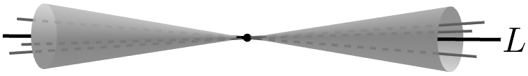
(a) $B^{-}_{r}(L)$ has $\{0\}$ and lines inside a double cone; $B^{+}_{r}(L)$ has $\mathds{R}^{3}$, lines and planes intercepting the cone interior; $B_{r}(L)$ has only lines.

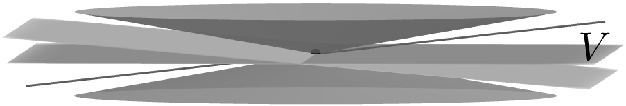
(b) $B^{-}_{r}(V)$ has $\{0\}$, lines and planes outside a double cone; $B^{+}_{r}(V)$ has $\mathds{R}^{3}$ and planes outside the cone; $B_{r}(V)$ has only planes.

Figure 1: Backward balls of small radius $r$ around a line $L$ and a plane $V$ in $G(\mathds{R}^{3})$

The subspace topology of $G_{p}^{n}$ (for $\tau^{\pm}$ or $\tau$) is its usual one, as in it $d$ is the original metric. The $G_{p}^{n}$’s are intricately connected to each other in $\tau^{\pm}$, while $\tau$ is the usual topology of their disjoint union, since $\hat{d}(V,W)=\Delta_{\max\{p,q\}}\geq 1$ for $V\in G_{p}^{n}$ and $W\in G_{q}^{n}$ with $p\neq q$.

Proposition 4.1.

$G^{n\pm}$ are compact, Smyth bicomplete and contractible.

Proof.

$\tau^{\pm}$ are coarser than $\tau$, which is compact. For small $\epsilon>0$ we have $d(V_{k},V_{l})<\epsilon\Rightarrow\dim V_{k}\leq\dim V_{l}$, so any left or right K-Cauchy sequence $V_{k}$ eventually becomes a Cauchy sequence in some $G_{p}^{n}$, which is complete. A contraction of $G^{n-}$ is given by $h(V,t)=\begin{cases}V&\text{if }t\in[0,\frac{1}{2}],\\ \{0\}&\text{if }t\in(\frac{1}{2},1],\end{cases}$ and in $G^{n+}$ we have the same with $[0,\frac{1}{2})$ and $[\frac{1}{2},1]$. ∎

In particular, this means $G^{n\pm}$ are path connected. Indeed, a path in $G^{n-}$ from $V\in G_{p}^{n}$ to $W\in G_{q}^{n}$, with $p\leq q$, is $\varphi(t)=\begin{cases}\phi(t)&\text{if }t\in[0,\frac{1}{2}),\\ W&\text{if }t\in[\frac{1}{2},1],\end{cases}$ where $\phi:[0,\frac{1}{2}]\rightarrow G_{p}^{n}$ is a path from $V$ to any $W^{\prime}\in G_{p}(W)$. The reversed path $\varphi(-t)$ links $W$ to $V$. In $G^{n+}$, use $[0,\frac{1}{2}]$ and $(\frac{1}{2},1]$.

Proposition 4.2.

$\alpha:G^{n}\rightarrow G^{n}$ given by $\alpha(V)=V^{\perp}$ is a bijective anti-isometry for asymmetric $\wedge$ or max metrics.

Proof.

For $V,W\neq\{0\}$ or $\mathds{F}^{n}$, the nonzero principal angles of $V^{\perp}$ and $W^{\perp}$ equal those of $V$ and $W$ [5]. Also, $\dim V=p>q=\dim W\Leftrightarrow\dim W^{\perp}=n-q>n-p=\dim V^{\perp}$, and for these metrics $\Delta_{n-q}=\Delta_{p}$. ∎

So $\alpha$ gives a self-homeomorphism of $G^{n}$, with $G_{p}^{n}\simeq G_{n-p}^{n}$ as usual, and a homeomorphism $G^{n+}\simeq G^{n-}$. The asymmetric $G^{n\pm}$ split, in a sense, the usual symmetry of $G^{n}$ (see Fig. 2, and compare with Examples 2.2 and 2.3). For asymmetric $l^{2}$ metrics and $n\geq 2$, $\alpha$ is not an anti-isometry, but gives the same homeomorphisms.

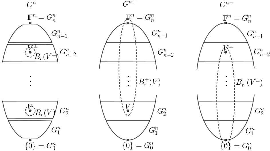
Figure 2: Natural topologies of the Total Grassmannian. The $G_{p}^{n}$’s are the connected components of $G^{n}$, but are intricately connected to each other in $G^{n\pm}$ (more so than the figure shows). The map $V\mapsto V^{\perp}$ is a symmetry of $G^{n}$, and flips $G^{n+}\leftrightarrow G^{n-}$, which are asymmetric, with balls $B_{r}^{\pm}(V)$ stretching upwards/downwards to include subspaces of larger/smaller dimension close to containing/being contained in $V$.

In what follows, $\mathds{F}\mathds{P}^{n-1}$ is the projective space of $\mathds{F}^{n}$, $\mathds{1}$ is the identity map (in $\mathds{F}^{n}$ or $G^{n}$), $\alpha$ is as above, and $M^{\pm}$ are as in Example 2.3.

Proposition 4.3.

$\operatorname{Isom}(G^{n})\cong\operatorname{Isom}(\mathds{F}\mathds{P}^{n-1})$.

Proof.

Any $f\in\operatorname{Isom}(G^{n})$ preserves the partial order $\subset$ of subspaces, so it preserves dimensions and restricts to an isometry of $G_{1}^{n}=\mathds{F}\mathds{P}^{n-1}$. And any $f\in\operatorname{Isom}(G_{1}^{n})$ extends uniquely to an $f:G^{n}\rightarrow G^{n}$ preserving $\subset$, and as it preserves angles between lines, this extension preserves principal angles between subspaces, hence is an isometry of $G^{n}$. ∎

Recall that $\operatorname{Isom}(\mathds{R}\mathds{P}^{n-1})=PO(n)=O(n)/\{\pm\mathds{1}\}$, while $\operatorname{Isom}(\mathds{C}\mathds{P}^{n-1})$ is generated by $PU(n)=U(n)/U(1)$ and complex conjugation [64].

Corollary 4.4.

$\operatorname{Transf}(G^{n})\cong\operatorname{Isom}(\mathds{F}\mathds{P}^{n-1})\rtimes\{\mathds{1},\alpha\}$ for asymmetric $\wedge$ or max metrics. For $l^{2}$ ones, $\operatorname{Transf}(G^{n})\cong\operatorname{Isom}(\mathds{F}\mathds{P}^{n-1})$ if $n\geq 2$, and $\operatorname{Transf}(G^{n})=\{\mathds{1},\alpha\}$ if $n=1$.

Proof.

In the $\wedge$ or $\max$ cases, the composition of $\alpha$ and any anti-isometry is an isometry. In the $l^{2}$ case with $n\geq 2$, as an anti-isometry $f$ would reverse $\subset$, and so $f(\{0\})=\mathds{F}^{n}$ and $f(L)\in G_{n-1}^{n}$ for $L\in G_{1}^{n}$, we would have $d(L,\{0\})=\Delta_{1}\neq\Delta_{n}=d(\mathds{F}^{n},f(L))$, a contradiction. ∎

Proposition 4.5.

$G^{n\pm}/\operatorname{Isom}(G^{n})\simeq M^{\pm}$.

Proof.

The orbits are the $G_{p}^{n}$’s, and $\pi:G^{n-}\rightarrow M^{-}$ given by $\pi(V)=\dim V$ is a quotient map, since both $\pi^{-1}(\{0,1,\ldots,p\})=\bigcup_{q\leq p}G_{q}^{n}$ and $\pi(B^{-}_{r}(V))=\{0,1,\ldots,\dim V\}$ are open. The proof for $G^{n+}$ is similar. ∎

4.1 Geodesics for asymmetric $l^{2}$ or $\wedge$ metrics

Let $d$ be an asymmetric $l^{2}$ or $\wedge$ metric (remember that geodesics of $G_{p}^{n}$ coincide for these), and $\varphi:I\rightarrow G^{n\pm}$ be a rectifiable curve.

Definition 4.6.

$c\in I$ is a critical point of $\varphi$ if for any $\delta>0$ there is $t\in(c-\delta,c+\delta)\cap I$ such that $\dim\varphi(t)\neq\dim\varphi(c)$.

Proposition 4.7.

$\varphi$ has finitely many critical points.

Proof.

Assuming otherwise, there are $t_{0}<t_{1}<t_{2}<\cdots$ in $I$ such that $\dim\varphi(t_{i})\neq\dim\varphi(t_{i+1})$, and passing to a subsequence we can assume $\dim\varphi(t_{2i})>\dim\varphi(t_{2i+1})$. But then $\ell_{\varphi}\geq\sum_{i}d(\varphi(t_{2i}),\varphi(t_{2i+1}))=\sum_{i}\Delta_{\dim\varphi(t_{2i})}=\infty$, contradicting the rectifiability of $\varphi$. ∎

So any $c\in I$ has a $\delta>0$ such that $\varphi$ restricted to $(c-\delta,c)$ is a curve in some $G_{p}^{n}$, where $\lim_{t\rightarrow c^{-}}\varphi(t)$ is well defined. Likewise, $\lim_{t\rightarrow c^{+}}\varphi(t)$ is well defined. Continuity implies $\lim_{t\rightarrow c^{\pm}}\varphi(t)\subset\varphi(c)$ in $G^{n-}$, and $\lim_{t\rightarrow c^{\pm}}\varphi(t)\supset\varphi(c)$ in $G^{n+}$.

Definition 4.8.

$\varphi$ expands (resp. contracts) from $U$ to $V$ at $c\in I$ if $U\subsetneq V$ (resp. $U\supsetneq V$) and either $\lim_{t\rightarrow c^{-}}\varphi(t)=U$ and $\varphi(c)=V$, or $\varphi(c)=U$ and $\lim_{t\rightarrow c^{+}}\varphi(t)=V$.

Critical points are those with expansions or contractions (possibly both, as in $\varphi:\mathds{R}\rightarrow G^{n-}$ with $\varphi(0)=\mathds{F}^{n}$, $\varphi(t)=\{0\}$ for $t\neq 0$).

Proposition 4.9.

If $\varphi$ expands (resp. contracts) from $U$ to $V$ at $c$, there is a partition $I=I_{1}\cup I_{2}$ with $\sup I_{1}=\inf I_{2}=c$ such that $\ell_{\varphi}=\ell_{\varphi\lvert_{I_{1}}}+\ell_{\varphi\lvert_{I_{2}}}$ (resp. $\ell_{\varphi}=\ell_{\varphi\lvert_{I_{1}}}+\ell_{\varphi\lvert_{I_{2}}}+\Delta\ell_{\varphi,c}$, where $\Delta\ell_{\varphi,c}=\Delta_{\dim U}$).

Proof.

If $\varphi(c)=V$, for $I_{1}=I\cap(-\infty,c)$ and $I_{2}=I\cap[c,\infty)$ we have $\ell_{\varphi}=\ell_{\varphi\lvert_{I_{1}}}+\ell_{\varphi\lvert_{I_{2}}}+\lim_{t\rightarrow c^{-}}d(\varphi(t),V)$. As $\varphi(t)$ converges to $U$ in a $G_{p}^{n}$, this limit is $d(U,V)$, so $0$ for an expansion, $\Delta_{p}$ for a contraction. If $\varphi(c)=U$, use $I_{1}=I\cap(-\infty,c]$, $I_{2}=I\cap(c,\infty)$ and $\lim_{t\rightarrow c^{+}}d(U,\varphi(t))$. ∎

The length discontinuity $\Delta\ell_{\varphi,c}$ at contractions might be useful in some applications as a sort of penalty for information loss. As its value depends on $d$, curve lengths and geodesics no longer coincide for all asymmetric $l^{2}$ or $\wedge$ metrics in $G^{n\pm}$.

Corollary 4.10.

A curve $\eta:I\rightarrow G^{n\pm}$ is null $\Leftrightarrow$ it is piecewise constant, changing at most by a finite number of expansions.

Proof.

($\Leftarrow$) Immediate. ($\Rightarrow$) $\eta$ can have no contraction, and in any interval with no expansion it is a null curve in some $G_{p}^{n}$, hence constant. ∎

Definition 4.11.

A path $\varphi:[a,b]\rightarrow G^{n\pm}$ from $V\in G_{p}^{n}$ to $W\in G_{q}^{n}$ is:

• type I if $\varphi(t)=\phi(t)\oplus\eta(t)$ for a minimal geodesic $\phi:[a,b]\rightarrow G_{p}^{n}$ from $V$ to a projection subspace $W^{\prime}$ of $W$ w.r.t. $V$, and a null path $\eta:[a,b]\rightarrow G^{n\pm}$ from $\{0\}$ to $W^{\prime\perp}\cap W$.

• type II if it has a contraction at some $c\in I$, with $\Delta\ell_{\varphi,c}=\Delta_{p}$, and is null in $[a,c)$ and $(c,b]$.

Type I paths exist $\Leftrightarrow p\leq q$ (so $W^{\prime}\in G_{p}^{n}$), and have length $d_{g}(V,W)$ (the asymmetric geodesic distance). Type II paths exist $\Leftrightarrow V\neq\{0\}$ (so $\varphi$ can contract from $V$ to $\{0\}$, then expand to $W$), and have length $\Delta_{p}$ (this $\Delta_{p}$ is w.r.t. $d$). See Fig. 3 for examples of such paths.

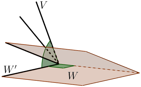
(a) Type I path from $V$ to $W$: $V$ rotates towards $W^{\prime}$, and along the way it expands to a plane that continues rotating to $W$.

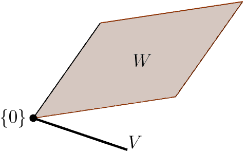
(b) Type II path from $W$ to $V$: it remains constant at $W$ for a while, then contracts to $\{0\}$, and later expands to $V$.

Figure 3: Type I and II paths between a line $V$ and a plane $W$ in $\mathds{R}^{3}$

Theorem 4.12.

For an asymmetric $l^{2}$ or $\wedge$ metric $d$, a path in $G^{n\pm}$ from $V\in G_{p}^{n}$ to $W\in G_{q}^{n}$ is a minimal geodesic $\Leftrightarrow$ it is type I and $d_{g}(V,W)\leq\Delta_{p}$, or it is type II and $\Delta_{p}\leq d_{g}(V,W)$.

Proof.

If $V=\{0\}$, the minimal geodesics are null paths from it to $W$ (type I with $\phi=\{0\}$). If $p>q$, any path $\varphi$ has at least one contraction, with $\ell_{\varphi}\geq\Delta\ell_{\varphi,c}\geq\Delta_{p}$, so the minimal geodesics are the type II paths, and $\Delta_{p}\leq\frac{\pi}{2}\sqrt{p}=d_{g}(V,W)$.

If $0<p\leq q$, any path $\varphi$ with $\ell_{\varphi}\leq\Delta_{p}$ has at most one contraction, being type II if it has one. Suppose it has none. If $p=q$, it is type I with $\eta=\{0\}$. If $p<q$, assume it has a single expansion (the general case follows via induction), from $U^{\prime}\in G_{p}^{n}$ to $U\in G_{q}^{n}$ at $c$. By Proposition 3.6, $\ell_{\varphi}\geq d_{g}(V,U^{\prime})+d_{g}(U,W)\geq d_{g}(V,U^{\prime})+d_{g}(U^{\prime},W)\geq d_{g}(V,W)$. If $\ell_{\varphi}=d_{g}(V,W)$, these are equalities, so $\varphi\lvert_{[a,c)}$ and $\varphi\lvert_{(c,b]}$ extend to minimal geodesics $\varphi_{1}:[a,c]\rightarrow G_{p}^{n}$ from $V$ to $U^{\prime}$, and $\varphi_{2}:[c,b]\rightarrow G_{q}^{n}$ from $U$ to $W$, Proposition 3.7 gives $U^{\prime\prime}=U^{\prime\perp}\cap U\subset W$, and $d_{g}(V,W)=d_{g}(V,U^{\prime})+d_{g}(U^{\prime},W)$. By the characterization of geodesics in Section 2.3, $\varphi_{2}=\varphi_{2}^{\prime}\oplus U^{\prime\prime}$ for a minimal geodesic $\varphi_{2}^{\prime}:[c,b]\rightarrow G_{p}^{n}$ from $U^{\prime}$ to $W^{\prime}=U^{\prime\prime\perp}\cap W$, which is a projection subspace of $W$ w.r.t. $U^{\prime}$. By Propositions 3.6 and 3.8, $d_{g}(V,W)=d_{g}(V,U^{\prime})+d_{g}(U^{\prime},W^{\prime})\geq d_{g}(V,W^{\prime})$ is an equality, $W^{\prime}$ is also a projection subspace of $W$ w.r.t. $V$, and $\varphi_{1}$ and $\varphi_{2}^{\prime}$ form a minimal geodesic $\phi:[a,b]\rightarrow G_{p}^{n}$ from $V$ to $W^{\prime}$. With $\eta(t)=\{0\}$ for $t\in[a,c)$, $\eta(t)=U^{\prime\prime}$ for $t\in(c,b]$, and $\eta(c)=\{0\}$ in $G^{n+}$ or $U^{\prime\prime}$ in $G^{n-}$, we have that $\varphi=\phi\oplus\eta$ is type I. ∎

Corollary 4.13.

$G^{n\pm}$ are geodesic spaces for $d$, and the intrinsic asymmetric metric is $D(V,W)=\min\{d_{g}(V,W),\Delta_{\dim V}\}$.

Proof.

For $0<p\leq q$, both types of path from $V\in G_{p}^{n}$ to $W\in G_{q}^{n}$ exist, and whichever is shorter is a minimal geodesic. If $p>q$, type II ones exist, and $\Delta_{p}\leq d_{g}(V,W)$. If $p=0$ we have null paths. ∎

4.2 Between-points for $d_{g}$

By Corollary 4.13, $d_{g}$ is intrinsic in $G^{n\pm}$, and so its minimal geodesics are segments. Thus any $U$ in a minimal geodesic from $V$ to $W$ is a between-point. As we will show, the converse also holds.

Proposition 4.14.

For distinct $U\in G_{r}^{n}$, $V\in G_{p}^{n}$ and $W\in G_{q}^{n}$, we have $d_{g}(V,W)=d_{g}(V,U)+d_{g}(U,W)$ in the following cases and no other:

1. $r\leq q<p$ and $U\subset W$;

2. $r<p\leq q$, $U\subset W$ and $V\perp W$;

3. $p\leq r\leq q$ and there are projection subspaces $U^{\prime},W^{\prime}$ of $U,W$ w.r.t. $V$ such that $U^{\prime}$ is in a minimal geodesic of $G_{p}^{n}$ from $V$ to $W^{\prime}$ and $U^{\prime\perp}\cap U\subset W^{\prime\perp}\cap W$.

Proof.

If $q<r$, the equality gives $d_{g}(V,U)+\frac{\pi}{2}\sqrt{r}=d_{g}(V,W)\leq\frac{\pi}{2}\sqrt{p}$, so either $r<p$ and $\sqrt{p}+\sqrt{r}=\sqrt{p}$, or $r=p$ and $V=U$, both impossible. If $r\leq q<p$, it gives $d_{g}(U,W)=0$, so $U\subset W$. If $r<p\leq q$, $\frac{\pi}{2}\sqrt{p}+d_{g}(U,W)=d_{g}(V,W)\leq\frac{\pi}{2}\sqrt{p}$, so $U\subset W$ and $V\perp W$. If $p\leq r\leq q$, for any projection $p$-subspaces $U^{\prime}$ of $U$ w.r.t. $V$, and $W^{\prime}$ of $W$ w.r.t. $U^{\prime}$, Proposition 3.6 gives $d_{g}(V,W)\leq d_{g}(V,W^{\prime})\leq d_{g}(V,U^{\prime})+d_{g}(U^{\prime},W^{\prime})=d_{g}(V,U)+d_{g}(U^{\prime},W)\leq d_{g}(V,U)+d_{g}(U,W)=d_{g}(V,W)$. These are equalities, so, by Propositions 3.7 and 3.8, $W^{\prime}$ is also a projection subspace of $W$ w.r.t. $V$, $U^{\prime}$ is in a minimal geodesic of $G_{p}^{n}$ from $V$ to $W^{\prime}$, and $U^{\prime\perp}\cap U\subset W$. Thus $P_{W}(U^{\prime})\perp U^{\prime\perp}\cap U$, and as $\dim W^{\prime}\leq q-(r-p)=\dim W-\dim(U^{\prime\perp}\cap U)$ we can assume $W^{\prime}$ was chosen orthogonal to $U^{\prime\perp}\cap U$. The converses are immediate. ∎

Corollary 4.15.

For $d_{g}$, $U$ is a between-point from $V$ to $W\Leftrightarrow$ $U$ is in a minimal geodesic of $G^{n\pm}$ from $V$ to $W$.

Proof.

($\Rightarrow$) For distinct $U,V,W$, a type II geodesic is given in i and ii above by contraction from $V$ to $V\cap U$, then expansions to $U$ and $W$. In iii, a type I is given by a geodesic of $G_{p}^{n}$ from $V$ to $U^{\prime}$, expansion to $U$, a geodesic of $G_{r}^{n}$ from $U$ to $W^{\prime}\oplus(U^{\prime\perp}\cap U)$, then expansion to $W$. ∎

Still, $G^{n}$ is not convex for $d_{g}$, as a minimal geodesic from $V$ to a distinct $W$ might have no other element. But this only happens when $V$ is a hyperplane of $W$, or when $V=\mathds{F}^{n}$ and $W=\{0\}$.

5 Asymmetric $\wedge$ metrics

Using Grassmann algebra (Appendix A), we show the asymmetric $\wedge$ metrics (Fubini-Study $d_{FS}$, chordal-$\wedge$ $d_{c\wedge}$ and Binet-Cauchy $d_{BC}$) have nice geometric interpretations, useful properties, and are easy to compute.

Definition 5.1.

Let $V,W\in G^{n}$, and $A\in\bigwedge\mathds{F}^{n}$ be a blade with $[A]=V$. The asymmetric angle from $V$ to $W$ is $\Theta_{V,W}=\cos^{-1}\frac{\|P_{W}A\|}{\|A\|}$.

Formerly called Grassmann angle [56], its links to products of Grassmann and Clifford algebras [57] give easy ways to compute it and nice properties [59]. For the contraction of nonzero blades $A,B\in\bigwedge\mathds{F}^{n}$,

$$\cos\Theta_{[A],[B]}=\frac{\|A\lrcorner\,B\|}{\|A\|\|B\|}\quad\left(=\frac{|\langle A,B\rangle|}{\|A\|\|B\|}\text{ if }\textstyle{A,B\in\bigwedge^{p}\mathds{F}^{n}}\right).$$ (1)

We can interpret it via projection factors [60]. Let $V_{\mathds{R}}$ ($=V$ if $\mathds{F}=\mathds{R}$) be the underlying real space of $V$, and $\operatorname{vol}_{k}$ be the $k$-dimensional volume.

Definition 5.2.

Let $V,W\in G^{n}$, $k=\dim V_{\mathds{R}}$, and $S\subset V$ be a set with $\operatorname{vol}_{k}(S)\neq 0$. The projection factor of $V$ on $W$ is $\pi_{V,W}=\frac{\operatorname{vol}_{k}(P_{W}(S))}{\operatorname{vol}_{k}(S)}$.

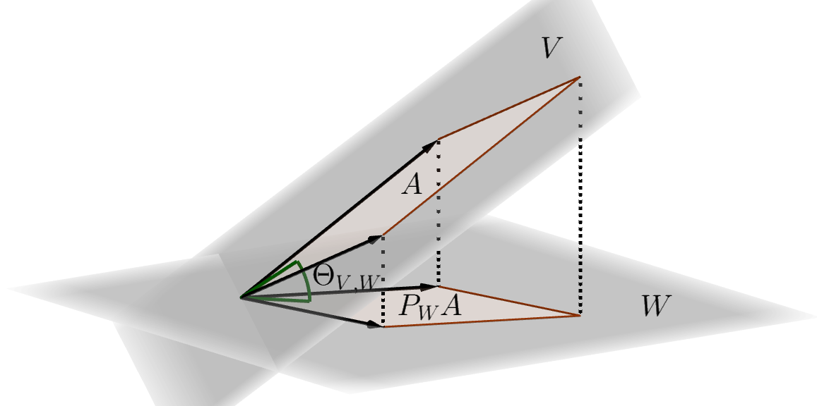
Figure 4: Orthogonal projection of a real 2-blade, $\cos\Theta_{V,W}=\frac{\|P_{W}A\|}{\|A\|}=\frac{\operatorname{area}(P_{W}A)}{\operatorname{area}(A)}$

As $\|A\|$ and $\|P_{W}A\|$ (squared, if $\mathds{F}=\mathds{C}$) are volumes of parallelotopes,

$$\cos\Theta_{V,W}=\begin{cases}\pi_{V,W}&\text{if $\mathds{F}=\mathds{R}$},\\ \sqrt{\pi_{V,W}}&\text{if $\mathds{F}=\mathds{C}$.}\end{cases}$$

In other words, $\cos\Theta_{V,W}$ (squared, if $\mathds{F}=\mathds{C}$) measures the contraction of volumes orthogonally projected from $V$ to $W$ (Fig. 4).

The asymmetric Fubini-Study metric (Table 1) is just this angle:

Proposition 5.3.

For $V\in G_{p}^{n}$ and $W\in G_{q}^{n}$,

$$d_{FS}(V,W)=\Theta_{V,W}=\begin{cases}0&\text{if }p=0,\\ \cos^{-1}\left(\prod_{i=1}^{p}\cos\theta_{i}\right)&\text{if }0<p\leq q,\\ \frac{\pi}{2}&\text{if }p>q,\end{cases}$$

where the $\theta_{i}$’s are the principal angles.

Proof.

If $V$ and $W$ have principal bases $(e_{1},\ldots,e_{p})$ and $(f_{1},\ldots,f_{q})$, for $A=e_{1}\wedge\cdots\wedge e_{p}$ we have $P_{W}A=0$ if $p>q$, otherwise $P_{W}e_{i}=f_{i}\,\cos\theta_{i}\ \forall i$ and so $P_{W}A=\cos\theta_{1}\cdots\cos\theta_{p}\,f_{1}\wedge\cdots\wedge f_{p}$. If $V\neq\{0\}$ and $W=\{0\}$ then $P_{W}A=0$. If $V=\{0\}=[1]$ we have $P_{W}1=1$. ∎

As $\Theta_{V,W}=\frac{\pi}{2}\Leftrightarrow V\simperp W$ ($\theta_{p}=\frac{\pi}{2}$ or $p>q$), the angle carries some dimensional data ($\Theta_{V,W}\neq\frac{\pi}{2}\Rightarrow\dim P_{W}(V)=\dim V\leq\dim W$). The asymmetry $\Theta_{V,W}\neq\Theta_{W,V}$ for $p\neq q$ reflects the dimensional asymmetry of subspaces, and is crucial for the oriented triangle inequality (Fig. 5) and even for the trivial $\Theta_{V,W}=\Theta_{V,P_{W}(V)}$: usual angles between the smaller subspace and its projection on the larger one [65] give $\frac{\pi}{2}$ for perpendicular planes $V,W\subset\mathds{R}^{3}$, but $0$ for $V$ and $P_{W}(V)$.

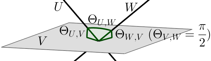
Figure 5: Oriented triangle inequality, $\Theta_{U,W}\leq\Theta_{U,V}+\Theta_{V,W}$ but $\Theta_{U,W}>\Theta_{U,V}+\Theta_{W,V}$

Proposition 5.4.

Extend an orthogonal basis $(w_{1},\ldots,w_{q})$ of $W\in G_{q}^{n}$ to another $\beta=(w_{1},\ldots,w_{n})$ of $\mathds{F}^{n}$. For $V\in G_{p}^{n}$,

$$d_{BC}(V,W)=\sin\Theta_{V,W}=\begin{cases}\left(1-\pi_{V,W}^{2}\right)^{\frac{1}{2}}=\left(\sum\pi_{V,U}^{2}\right)^{\frac{1}{2}}&\text{if }\mathds{F}=\mathds{R},\\ \left(1-\pi_{V,W}\right)^{\frac{1}{2}}=\left(\sum\pi_{V,U}\right)^{\frac{1}{2}}&\text{if }\mathds{F}=\mathds{C},\end{cases}$$

where the sums run over all coordinate $p$-subspaces $U$ of $\beta$ with $U\not\subset W$.

Proof.

Assume $\beta$ is orthonormal. For a unit $A\in\bigwedge^{p}V$, Proposition 5.3 and $d_{BC}$ in Table 1 give $d_{BC}^{2}(V,W)=1-\cos^{2}\Theta_{V,W}=\|A\|^{2}-\|P_{W}A\|^{2}=\sum\limits_{1\leq i_{1}<\cdots<i_{p}\leq n}|\langle w_{i_{1}}\wedge\cdots\wedge w_{i_{p}},A\rangle|^{2}-\sum\limits_{1\leq i_{1}<\cdots<i_{p}\leq q}|\langle w_{i_{1}}\wedge\cdots\wedge w_{i_{p}},A\rangle|^{2}=\sum_{\begin{subarray}{c}1\leq i_{1}<\cdots<i_{p}\leq n,\\ i_{j}>q\text{ for some }j\end{subarray}}\|P_{[w_{i_{1}}\wedge\cdots\wedge w_{i_{p}}]}A\|^{2}$. ∎

So $d_{BC}^{2}(V,W)$ is the sum of volumes (squared if $\mathds{F}=\mathds{R}$) of projections of a unit volume of $V$ on all coordinate $p$-subspaces not contained in $W$ (Fig. 6). If $p>q$, no $p$-subspace is contained in $W$, and $d_{BC}(V,W)=1$ corresponds to volumetric Pythagorean theorems [60].

We also have $d_{c\wedge}(V,W)=2\sin\frac{\Theta_{V,W}}{2}=\begin{cases}\sqrt{2-2\pi_{V,W}}&\text{if $\mathds{F}=\mathds{R}$},\\ \sqrt{2-2\sqrt{\pi_{V,W}}}&\text{if $\mathds{F}=\mathds{C}$.}\end{cases}$

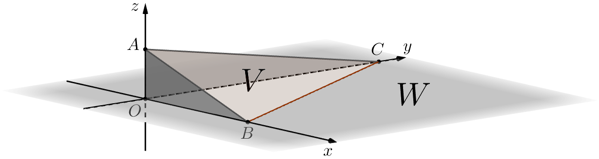
Figure 6: $d_{FS}(V,W)=\cos^{-1}\left(\frac{\operatorname{area}(OBC)}{\operatorname{area}(ABC)}\right)$ describes the separation between $V$ (plane of $ABC$) and $W$ in terms of how areas of $V$ contract if orthogonally projected on $W$; $d_{BC}(V,W)=\left(\frac{\operatorname{area}^{2}(OAB)+\operatorname{area}^{2}(OAC)}{\operatorname{area}^{2}(ABC)}\right)^{\frac{1}{2}}$ uses areas of vertical triangles that ‘lift’ $V$; $d_{c\wedge}(V,W)=\left(2\frac{\operatorname{area}(ABC)-\operatorname{area}(OBC)}{\operatorname{area}(ABC)}\right)^{\frac{1}{2}}$ shows how much area $ABC$ loses if projected.

Proposition 5.5.

$\cos^{2}\Theta_{V,W}=\det(\mathbf{P}^{\dagger}\mathbf{P})$, where $\mathbf{P}$ is a matrix for the orthogonal projection $V\rightarrow W$ in orthonormal bases of $V$ and $W$, and ^† is the conjugate transpose. If $\dim V=\dim W$, $\cos\Theta_{V,W}=|\det\mathbf{P}|$.

Proof.

Follows from Proposition 5.3, as in principal bases $\mathbf{P}$ is a $q\times p$ diagonal matrix with the $\cos\theta_{i}$’s. ∎

Proposition 5.6.

Given any bases $(v_{1},\ldots,v_{p})$ of $V$ and $(w_{1},\ldots,w_{q})$ of $W$, let $\mathbf{A}=\big{(}\langle v_{i},v_{j}\rangle\big{)}$, $\mathbf{B}=\big{(}\langle w_{i},w_{j}\rangle\big{)}$ and $\mathbf{C}=\big{(}\langle w_{i},v_{j}\rangle\big{)}$. Then

$$\cos^{2}\Theta_{V,W}=\frac{\det(\mathbf{C}^{\dagger}\mathbf{B}^{-1}\mathbf{C})}{\det\mathbf{A}}.$$ (2)

When $p=q$, $\cos\Theta_{V,W}=\frac{|\det\mathbf{C}\,|}{\sqrt{\det\mathbf{A}\cdot\det\mathbf{B}}}$.

Proof.

If $p>q$ then $\Theta_{V,W}=\frac{\pi}{2}$, and $\det(\mathbf{C}^{\dagger}\mathbf{B}^{-1}\mathbf{C})=0$ as it is a $p\times p$ matrix with at most rank $q$. If $p\leq q$, Laplace expansion w.r.t. columns $q+1,\ldots,q+p$ of the $(q+p)\times(q+p)$ block matrix $\mathbf{M}=\begin{pmatrix}\mathbf{B}&\mathbf{C}\\ \mathbf{C}^{\dagger}&\mathbf{0}\end{pmatrix}$ gives $\det\mathbf{M}=\sum_{\mathbf{i}}(-1)^{pq+\frac{p(p+1)}{2}+i_{1}+\cdots+i_{p}}\cdot\det\mathbf{C}_{\mathbf{i}}\cdot\det\mathbf{N}_{\mathbf{i}^{\prime}}$, where the sum runs over all $\mathbf{i}=(i_{1},\ldots,i_{p})$ with $1\leq i_{1}<\cdots<i_{p}\leq q$, $\mathbf{C}_{\mathbf{i}}$ is the $p\times p$ submatrix of $\mathbf{M}$ formed by lines of $\mathbf{C}$ with indices in $\mathbf{i}$, and $\mathbf{N}_{\mathbf{i}^{\prime}}=\begin{pmatrix}\mathbf{B}_{\mathbf{i}^{\prime}}\\[1.0pt] \mathbf{C}^{\dagger}\end{pmatrix}$ is its $q\times q$ complementary submatrix, formed by lines of $\mathbf{B}$ with indices not in $\mathbf{i}$ and all of $\mathbf{C}^{\dagger}$. For $A=v_{1}\wedge\cdots\wedge v_{p}$ and $B=w_{1}\wedge\cdots\wedge w_{q}$, Proposition A.2 gives $\|A\lrcorner\,B\|^{2}=\langle A\wedge(A\lrcorner\,B),B\rangle=\sum_{\mathbf{i}}\epsilon_{\mathbf{i}\mathbf{i}^{\prime}}\,\langle B_{\mathbf{i}},A\rangle\,\langle A\wedge B_{\mathbf{i}^{\prime}},B\rangle$. As $\det\mathbf{C}_{\mathbf{i}}=\langle B_{\mathbf{i}},A\rangle$ and $\det\mathbf{N}_{\mathbf{i}^{\prime}}=\langle B_{\mathbf{i}^{\prime}}\wedge A,B\rangle=(-1)^{pq+p}\langle A\wedge B_{\mathbf{i}^{\prime}},B\rangle$, we obtain $\|A\lrcorner\,B\|^{2}=(-1)^{p}\det\mathbf{M}$, so that $\cos^{2}\Theta_{V,W}=\frac{(-1)^{p}\det\mathbf{M}}{\det\mathbf{A}\cdot\det\mathbf{B}}$, by (1). The result follows from Schur’s determinant identity. ∎

Example 5.7.

Let $(f_{1},\ldots,f_{5})$ be the canonical basis of $\mathds{R}^{5}$, $e_{1}=\frac{\sqrt{3}f_{1}+f_{4}}{2}$, $e_{2}=\frac{f_{2}+f_{5}}{\sqrt{2}}$, $V=\operatorname{span}\{e_{1},e_{2}\}$ and $W=\operatorname{span}\{f_{1},f_{2},f_{3}\}$. Principal angles are $30^{\circ}$ and $45^{\circ}$, so $\Theta_{V,W}=\cos^{-1}(\frac{\sqrt{3}}{2}\cdot\frac{\sqrt{2}}{2})\cong 52^{\circ}$ and areas in $V$ shrink by $\frac{\sqrt{6}}{4}$ if orthogonally projected on $W$. Volumes in $W$ vanish if projected on $V$, so $\Theta_{W,V}=90^{\circ}$. Also, $\pi_{V,[f_{1}\wedge f_{5}]}=\frac{\sqrt{6}}{4}$, $\pi_{V,[f_{2}\wedge f_{4}]}=\pi_{V,[f_{4}\wedge f_{5}]}=\frac{\sqrt{2}}{4}$ and $\pi_{V,[f_{1}\wedge f_{4}]}=\pi_{V,[f_{2}\wedge f_{5}]}=\pi_{V,[f_{3}\wedge f_{4}]}=\pi_{V,[f_{3}\wedge f_{5}]}=0$, so $d_{BC}(V,W)=\sin\Theta_{V,W}=\sqrt{\frac{5}{8}}=\sqrt{\sum_{\begin{subarray}{c}1\leq i<j\leq 5,\{i,j\}\not\subset\{1,2,3\}\end{subarray}}\pi_{V,[f_{i}\wedge f_{j}]}^{2}}$.

Example 5.8.

If $(u_{1},\ldots,u_{5})$ is the canonical basis of $\mathds{R}^{5}$, $v_{1}=2u_{1}-u_{2}$, $v_{2}=2u_{1}+u_{3}$, $w_{1}=u_{2}+u_{5}$, $w_{2}=u_{3}-u_{4}$, $w_{3}=u_{4}$, $V=\operatorname{span}\{v_{1},v_{2}\}$ and $W=\operatorname{span}\{w_{1},w_{2},w_{3}\}$, then $\mathbf{A}=\begin{pmatrix}5&4\\ 4&5\end{pmatrix}$, $\mathbf{B}=\begin{pmatrix}2&0&0\\ 0&2&-1\\ 0&-1&1\end{pmatrix}$, $\mathbf{C}=\begin{pmatrix}-1&0\\ 0&1\\ 0&0\end{pmatrix}$ and (2) gives $\Theta_{V,W}=\cos^{-1}\frac{1}{3\sqrt{2}}\cong 76.4^{\circ}$. Switching $V$ and $W$, we have $\mathbf{A}=\begin{pmatrix}2&0&0\\ 0&2&-1\\ 0&-1&1\end{pmatrix}$, $\mathbf{B}=\begin{pmatrix}5&4\\ 4&5\end{pmatrix}$, $\mathbf{C}=\begin{pmatrix}-1&0&0\\ 0&1&0\end{pmatrix}$, and so $\Theta_{W,V}=90^{\circ}$, as expected. Calculations with Grassmann algebra are easier: writing $u_{13}=u_{1}\wedge u_{3}$ for example, we have $V=[A]$ for $A=v_{12}=2u_{12}+2u_{13}-u_{23}$ and $W=[B]$ for $B=w_{123}=u_{234}+u_{345}$, so $\|A\|=3$, $\|B\|=\sqrt{2}$, $A\lrcorner\,B=-u_{4}$ and $B\lrcorner\,A=0$, and (1) gives the same results.

Example 5.9.

In $\mathds{C}^{3}$, let $v=(1,0,\mathrm{i})$, $w_{1}=(1,0,0)$, $w_{2}=(\mathrm{i},1,0)$, $V=\operatorname{span}\{v\}$ and $W=\operatorname{span}\{w_{1},w_{2}\}$. Then $\mathbf{A}=(2)$, $\mathbf{B}=\begin{pmatrix}1&\mathrm{i}\\ -\mathrm{i}&2\end{pmatrix}$, $\mathbf{C}=\begin{pmatrix}1\\ -\mathrm{i}\end{pmatrix}$, and we obtain $\Theta_{V,W}=45^{\circ}$. Identifying $\mathds{C}^{3}$ with $\mathds{R}^{6}$, we have $V_{\mathds{R}}=\operatorname{span}_{\mathds{R}}\{v,\mathrm{i}v\}$ and $W_{\mathds{R}}=\operatorname{span}_{\mathds{R}}\{w_{1},\mathrm{i}w_{1},w_{2},\mathrm{i}w_{2}\}$, with

$$v =(1,0,0,0,0,1), w_{1} =(1,0,0,0,0,0), w_{2} =(0,1,1,0,0,0),$$

$$\mathrm{i}v =(0,1,0,0,-1,0), \mathrm{i}w_{1} =(0,1,0,0,0,0), \mathrm{i}w_{2} =(-1,0,0,1,0,0),$$

so now $\mathbf{A}=\begin{pmatrix}2&0\\ 0&2\end{pmatrix}$, $\mathbf{B}=\begin{pmatrix}1&0&0&-1\\ 0&1&1&0\\ 0&1&2&0\\ -1&0&0&2\end{pmatrix}$, $\mathbf{C}=\begin{pmatrix}1&0\\ 0&1\\ 0&1\\ -1&0\end{pmatrix}$ and $\Theta_{V_{\mathds{R}},W_{\mathds{R}}}=60^{\circ}$. Note that $\Theta_{V_{\mathds{R}},W_{\mathds{R}}}\neq\Theta_{V,W}$ as they convey in different ways that areas in $V$ contract by $\pi_{V_{\mathds{R}},W_{\mathds{R}}}=\pi_{V,W}=\frac{1}{2}$ if orthogonally projected on $W$.

5.1 Between-points for $d_{FS}$

Here we show, for $d_{FS}$, that between-points are in minimal geodesics, and determine when these are segments.

Proposition 5.10.

$d_{FS}(V,W)=d_{FS}(V,U)+d_{FS}(U,W)$ for $U,V,W\in G^{n}$ in the following cases and no other:

1. $U\subset W$, with $V\simperp W$ or $P_{W}(V)\subset U$;

2. $V\subset U$, with $V\simperp W$ or $V^{\perp}\cap U\subset W$;

3. $V=[v]\oplus R$, $U=[u]\oplus S$ and $W=[w]\oplus T$ for subspaces $R\subset S\subset T$ and aligned  nonzero $u,v,w\in T^{\perp}$ with $u=\kappa v+\lambda w$ for $\kappa,\lambda>0$.

Proof.

By Proposition 3.9, case i corresponds to $\Theta_{U,W}=0$ and $\Theta_{V,W}=\Theta_{V,U}$, and ​ii to $\Theta_{V,U}=0$ and $\Theta_{V,W}=\Theta_{U,W}$. In ​6, Proposition B.3 gives $\Theta_{V,W}=\theta_{v,w}=\theta_{v,u}+\theta_{u,w}=\Theta_{V,U}+\Theta_{U,W}$.

If $\Theta_{V,W}=\Theta_{V,U}+\Theta_{U,W}$ with $\Theta_{V,U},\Theta_{U,W}\neq 0$ then $\Theta_{V,U},\Theta_{U,W}\neq\frac{\pi}{2}$, and so $V,U^{\prime},W^{\prime}\in G_{p}^{n}$ for some $p$, where $U^{\prime}=P_{U}(V)$ and $W^{\prime}=P_{W}(U^{\prime})$. By Proposition 3.6, $\Theta_{V,W}\leq\Theta_{V,W^{\prime}}\leq\Theta_{V,U^{\prime}}+\Theta_{U^{\prime},W^{\prime}}=\Theta_{V,U}+\Theta_{U^{\prime},W}\leq\Theta_{V,U}+\Theta_{U,W}$. These are equalities, so $\Theta_{U^{\prime},W^{\prime}}=\Theta_{U,W}\neq 0$, $\Theta_{V,W^{\prime}}\neq 0$, and $V$, $U^{\prime}$, $W^{\prime}$ are distinct. Proposition B.5 gives $R\in G_{p-1}^{n}$ and aligned $u,v,w\in R^{\perp}$ with $u=\kappa v+\lambda w$ for $\kappa,\lambda>0$, $U^{\prime}=[u]\oplus R$, $V=[v]\oplus R$ and $W^{\prime}=[w]\oplus R$. For $S^{\prime}=U^{\prime\perp}\cap U$ we have $u,v\perp S^{\prime}$, $w=\frac{u-\kappa v}{\lambda}\perp S^{\prime}$, and $S^{\prime}\subset W$ by Proposition 3.9, as $\Theta_{U^{\prime},W}=\Theta_{U,W}\neq\frac{\pi}{2}$. For $T^{\prime}=([w]\oplus R\oplus S^{\prime})^{\perp}\cap W$, as $P_{W}u\in W^{\prime}=[w]\oplus R$ we have $u,w\perp T^{\prime}$ and $v=\frac{u-\lambda w}{\kappa}\perp T^{\prime}$. So 6 is satisfied with $S=R\oplus S^{\prime}$ and $T=R\oplus S^{\prime}\oplus T^{\prime}$. ∎

Corollary 5.11.

For $d_{FS}$, if $U$ is a between-point from $V$ to $W$ then $U$ is in a minimal geodesic of $G^{n\pm}$ from $V$ to $W$.

Proof.

If $V\simperp W$ with $U\subset W$ or $V\subset U$, one can find a type II geodesic from $V$ to $W$ through $U$. If $V\not\simperp W$ then $P_{W}(V)$ is a projection subspace of $W$ w.r.t. $V$, so if $P_{W}(V)\subset U\subset W$, or if $V\subset U$ and $V^{\perp}\cap U\subset W$, one can find both types of path (unless $V=\{0\}$), and the shorter one is a geodesic. In case 6 above one can find a type I geodesic. ∎

The converse does not hold. In fact, $G^{n}$ is not convex for $d_{FS}$, and between-points exist only in the following cases:

Corollary 5.12.

For $d_{FS}$, there is a distinct between-point from $V\in G_{p}^{n}$ to $W\in G_{q}^{n}\Leftrightarrow V\simperp W$ with $V\neq\mathds{F}^{n}$ or $W\neq\{0\}$, or $W\simperp V$ with $V\not\subset W$, or $p\leq q-2$, or $p=q=\dim(V\cap W)+1$.

Proof.

($\Leftarrow$) Each case holds with: any $U\varsubsetneq W$ or $U\varsupsetneq V$; $U=P_{W}(V)$ ($\neq W$ as $W\simperp V$); $P_{W}(V)\subsetneq U\subsetneq W$; $U$ as in Proposition B.5. ($\Rightarrow$) If $V\not\simperp W$, case i above gives $P_{W}(V)\subset U\varsubsetneq W$, so $W\simperp V$, and $p\leq q-2$ if $V\subset W$; ii gives $V\varsubsetneq U$ and $V^{\perp}\cap U\subset W$, which imply the same; and 6 also implies the same if $R\neq T$, otherwise gives the last possibility. ∎

Minimal geodesics are segments in even less cases:

Proposition 5.13.

For $d_{FS}$, $G^{n\pm}$ has a segment from $V\in G_{p}^{n}$ to $W\in G_{q}^{n}\Leftrightarrow$ $V\simperp W$ or $p\leq\dim(V\cap W)+1$.

Proof.

By Corollary 4.13, a minimal geodesic $\varphi$ from $V$ to $W$ has $\ell_{\varphi}=\min\{d_{g}(V,W),\frac{\pi}{2}\}\geq d_{FS}(V,W)$. We have $d_{FS}(V,W)=\frac{\pi}{2}\Leftrightarrow V\simperp W$. If $V\not\simperp W$ then $p\leq q$ and, for a projection subspace $W^{\prime}$ of $W$ w.r.t. $V$, $d_{FS}(V,W)=d_{g}(V,W)\Leftrightarrow d_{FS}(V,W^{\prime})=d_{g}(V,W^{\prime})\Leftrightarrow\dim(V\cap W)=\dim(V\cap W^{\prime})\geq p-1$, by Proposition B.2. ∎

If $V=\mathds{F}^{n}$ and $W=\{0\}$, the segment is type II with no other points. If $V\simperp W$ with $p=q>\dim(V\cap W)+1$, by Corollary B.6 there is no segment in $G_{p}^{n}$, yet there is a type II segment in $G^{n\pm}$.

6 Final remarks

The definition of $d(V,W)$ in Theorem 3.4 uses the infimum taken in $[0,\Delta_{p}]$, which is natural as it is the smallest interval with all possible values of $d_{p}(V,U)$. But it can be tweaked for certain purposes: with $[0,\Delta_{n}]$, Proposition 4.2 extends for asymmetric $l^{2}$ metrics; with $[0,\infty]$ we have $d(V,W)=\infty$ if $\dim V>\dim W$, which may be useful in applications where dimensions can increase but not decrease (one might also use run-continuous paths, whose length varies continuously [54]).

Symmetrizing the asymmetric metrics of Table 1 via different norms yields new metrics, but information is lost. Max-symmetrized ones are trivial for distinct dimensions, but can still be useful: e.g., $\hat{\Theta}_{V,W}=\max\{\Theta_{V,W},\Theta_{W,V}\}$ gives $|\langle A,B\rangle|=\|A\|\|B\|\cos\hat{\Theta}_{[A],[B]}$ for any blades [57]. A min-symmetrization $\check{d}(V,W)=\min\{d(V,W),d(W,V)\}$ gives the distance from the smaller subspace to its projection on the larger one, which seems natural and is used in [22, 23, 24] and for angles [65]. But it fails the triangle inequality, and balls $\check{B}_{r}(V)=\{U\in G^{n}:\check{d}(U,V)<r\}$, with subspaces of all dimensions close to $V$, do not give a topology.

Under some conditions, high dimensional asymmetric metric spaces with measure are nearly symmetric [46], i.e. most pairs $(x,y)$ have small asymmetry $|d(x,y)-d(y,x)|$. This seems to be the case with $(G^{n},d_{FS})$ for large $n$. Each $G_{p}^{n}$ has a natural measure given by the action of the unitary group, and taking their dimensions $p(n-p)$ as relative weights we obtain a Borel measure in $G^{n}$. Most pairs of subspaces should have a considerable number of non-negligible principal angles, and so $d_{FS}(V,W)\cong\frac{\pi}{2}\cong d_{FS}(W,V)$, as $d_{FS}\rightarrow\frac{\pi}{2}$ quickly if several $\theta_{i}$’s are large, or a large number of them are not too small. This may render $d_{FS}$ unsuitable for some uses, but is important for quantum decoherence [66], allowing quantum states of many particles to quickly become nearly orthogonal. As decoherence is deemed responsible for the quantum-classical transition as the dimension of the quantum state space increases, this begs the question of whether this transition might be linked to a loss of asymmetry. As far as we know, there have been no attempts to relate quantum theory to asymmetric metric spaces. But it would not be so surprising to find a link, since fermionic Fock space is a Grassmann algebra, the Fubini-Study distance arises naturally in the theory, and $\Theta_{V,W}$ has led to complex Pythagorean theorems [60] with unexpected links to quantum probabilities [61].

Appendix A Grassmann exterior algebra

Grassmann algebra [2, 58] is a natural formalism to use with subspaces. For $X\in G_{r}^{n}$, it is a graded algebra $\bigwedge X=\bigoplus_{p\in\mathds{Z}}\bigwedge^{p}X$ with $\bigwedge^{0}X=\mathds{F}$, $\bigwedge^{1}X=X$ and $\bigwedge^{p}X=\{0\}$ if $p\not\in[0,r]$. For $A\in\bigwedge^{p}X$ and $B\in\bigwedge^{q}X$, its bilinear associative exterior product $\wedge$ satisfies $A\wedge B=(-1)^{pq}B\wedge A\in\bigwedge^{p+q}X$. For $u,v\in X$, $u\wedge v=-v\wedge u$, and so $v\wedge v=0$. For $p>0$, elements of $\bigwedge^{p}X$ are linear combinations of $p$-blades $B=v_{1}\wedge\cdots\wedge v_{p}$ for $v_{1},\ldots,v_{p}\in X$. If $B\neq 0$, $[B]=\{v\in X:v\wedge B=0\}=\operatorname{span}\{v_{1},\ldots,v_{p}\}$ is a $p$-subspace. Any $\lambda\in\mathds{F}$ is a $0$-blade with $[\lambda]=\{0\}$. For nonzero blades $A,B\in\bigwedge X$, if $[A]$ and $[B]$ are disjoint then $[A\wedge B]=[A]\oplus[B]$, otherwise $A\wedge B=0$. In the following known result, $A$ and $B$ need not be blades.

Proposition A.1.

Let $A\in\bigwedge V$ and $B\in\bigwedge W$ for disjoint $V,W\in G^{n}$. Then $A\wedge B=0\Leftrightarrow A=0$ or $B=0$.

The inner product $\langle A,B\rangle=\det\!\big{(}\langle v_{i},w_{j}\rangle\big{)}$ of $A=v_{1}\wedge\cdots\wedge v_{p}$ and $B=w_{1}\wedge\cdots\wedge w_{p}$ is extended linearly (sesquilinearly, if $\mathds{F}=\mathds{C}$), with distinct $\bigwedge^{p}X$’s being orthogonal. If $\mathds{F}=\mathds{R}$, $\|A\|=\sqrt{\langle A,A\rangle}$ is the $p$-dimensional volume of the parallelotope spanned by $v_{1},\ldots,v_{p}$. If $\mathds{F}=\mathds{C}$, $\|A\|^{2}$ is the $2p$-dimensional volume of that spanned by $v_{1},\mathrm{i}v_{1},\ldots,v_{p},\mathrm{i}v_{p}$. If $V\in G_{p}(X)$ has orthonormal basis $\{v_{1},\ldots,v_{p}\}$, $\bigwedge^{k}V$ has $\{v_{i_{1}}\wedge\cdots\wedge v_{i_{k}}:1\leq i_{1}<\cdots<i_{k}\leq p\}$, and $\bigwedge^{p}V=\operatorname{span}\{v_{1}\wedge\cdots\wedge v_{p}\}$ is a line in $\bigwedge X$. The orthogonal projection $P_{V}:X\rightarrow V$ extends to another $P_{V}:\bigwedge X\rightarrow\bigwedge V$, with $P_{V}(A\wedge B)=P_{V}A\wedge P_{V}B$ for $A,B\in\bigwedge X$.

The contraction $A\lrcorner\,B\in\bigwedge^{q-p}X$ of $A\in\bigwedge^{p}X$ and $B\in\bigwedge^{q}X$ is defined by $\langle C,A\lrcorner\,B\rangle=\langle A\wedge C,B\rangle$ for all $C\in\bigwedge^{q-p}X$. It is asymmetric, with $A\lrcorner\,B=0$ if $p>q$, and $A\lrcorner\,B=\langle A,B\rangle$ if $p=q$.

Proposition A.2 (​​[67]).

$A\lrcorner\,B=\sum_{\mathbf{i}}\epsilon_{\mathbf{i}\mathbf{i}^{\prime}}\,\langle A,B_{\mathbf{i}}\rangle\,B_{\mathbf{i}^{\prime}}$ for $A\in\bigwedge^{p}X$ and $B=w_{1}\wedge\cdots\wedge w_{q}\in\bigwedge^{q}X$ with $0<p<q$, where the sum is over all $\mathbf{i}=(i_{1},\ldots,i_{p})$ with $1\leq i_{1}<\cdots<i_{p}\leq q$, $B_{\mathbf{i}}=w_{i_{1}}\wedge\cdots\wedge w_{i_{p}}$, likewise for $B_{\mathbf{i}^{\prime}}$ with $\mathbf{i}^{\prime}=(1,\ldots,q)-\mathbf{i}$ (indices not in $\mathbf{i}$), and  $\epsilon_{\mathbf{i}\mathbf{i}^{\prime}}=(-1)^{\frac{p(p+1)}{2}+i_{1}+\cdots+i_{p}}$.

Appendix B Metrics in Grassmannians $G_{p}^{n}$

The main metrics used in $G_{p}^{n}$ [5, 6, 7, 8] derive from distances between lines. If $K=\operatorname{span}\{u\}$ and $L=\operatorname{span}\{v\}$ for aligned unit $u$ and $v$, their angular, chordal and gap distances are $\theta_{K,L}=\theta_{u,v}$, $c_{K,L}=\|u-v\|=2\sin\frac{\theta_{u,v}}{2}$ and $g_{K,L}=\|u-P_{L}u\|=\sin\theta_{u,v}$, respectively. The metrics are organized in Table 2 and described below for $V,W\in G_{p}^{n}$ with principal angles $\theta_{1}\leq\cdots\leq\theta_{p}$ and principal bases $(e_{1},\ldots,e_{p})$ and $(f_{1},\ldots,f_{p})$, whose vectors are used as columns of $n\times p$ matrices $\mathbf{E}$ and $\mathbf{F}$.

Type	angular	chordal	gap
$l^{2}$	$d_{g}=\sqrt{\sum_{i=1}^{p}\theta_{K_{i},L_{i}}^{2}}$	$d_{cF}=\sqrt{\sum_{i=1}^{p}c_{K_{i},L_{i}}^{2}}$	$d_{pF}=\sqrt{\sum_{i=1}^{p}g_{K_{i},L_{i}}^{2}}$
$\wedge$	$d_{FS}=\theta_{K_{\wedge},L_{\wedge}}$	$d_{c\wedge}=c_{K_{\wedge},L_{\wedge}}$	$d_{BC}=g_{K_{\wedge},L_{\wedge}}$
max	$d_{A}=\theta_{K_{p},L_{p}}$	$d_{c2}=c_{K_{p},L_{p}}$	$d_{p2}=g_{K_{p},L_{p}}$

Table 2: Metrics in $G_{p}^{n}$ in terms of angular, chordal or gap distances between lines $K_{i}=\operatorname{span}\{e_{i}\}$ and $L_{i}=\operatorname{span}\{f_{i}\}$, or $K_{\wedge}=\bigwedge^{p}V$ and $L_{\wedge}=\bigwedge^{p}W$

The $l^{2}$ metrics use the $l^{2}$ norm of the vector formed by the distances of lines $K_{i}=\operatorname{span}\{e_{i}\}$ and $L_{i}=\operatorname{span}\{f_{i}\}$ for $1\leq i\leq p$:

• Geodesic [3, 4]: $d_{g}=\sqrt{\sum_{i=1}^{p}\theta_{i}^{2}}$, geodesic distance of the unique Riemannian metric invariant by unitary maps, given by the Hilbert-Schmidt product in the tangent space $\operatorname{Hom}(V,V^{\perp})$ at $V$.

• Chordal Frobenius or Procrustes [6, 15]: embedding $G_{p}^{n}$ in the set of $n\times p$ matrices with Frobenius norm $\|\cdot\|_{F}$, $d_{cF}=\|\mathbf{E}-\mathbf{F}\|_{F}=\sqrt{\sum_{i=1}^{p}\|e_{i}-f_{i}\|^{2}}=2\sqrt{\sum_{i=1}^{p}\sin^{2}\frac{\theta_{i}}{2}}$.

• Projection Frobenius or chordal [15, 14, 13]: embedding $G_{p}^{n}$ in the set of projection matrices with $\|\cdot\|_{F}$, we have $d_{pF}=\frac{1}{\sqrt{2}}\|P_{V}-P_{W}\|_{F}=\sqrt{\sum_{i=1}^{p}\|e_{i}-P_{W}e_{i}\|^{2}}=\sqrt{\sum_{i=1}^{p}\sin^{2}\theta_{i}}$.

The $\wedge$ metrics use distances in $\bigwedge\mathds{F}^{n}$ of lines $K_{\wedge}=\bigwedge^{p}V=\operatorname{span}\{A\}$ and $L_{\wedge}=\bigwedge^{p}W=\operatorname{span}\{B\}$, for $A=e_{1}\wedge\cdots\wedge e_{p}$ and $B=f_{1}\wedge\cdots\wedge f_{p}$:

• Fubini-Study [11, 7, 24]: $d_{FS}=\theta_{A,B}=\cos^{-1}(\prod_{i=1}^{p}\cos\theta_{i})$, geodesic distance through $\mathds{P}(\bigwedge^{p}\mathds{F}^{n})$ (see Section B.1).

• Chordal $\wedge$: $d_{c\wedge}=\|A-B\|=2\sin\frac{\theta_{A,B}}{2}=\sqrt{2-2\prod_{i=1}^{p}\cos\theta_{i}}$.

• Binet-Cauchy [15, 20]: given by $d_{BC}=\|A-P_{W}A\|=\sin\theta_{A,B}=\sqrt{1-\prod_{i=1}^{p}\cos^{2}\theta_{i}}$.

The max metrics use maximum distances of $K_{i}$ and $L_{i}$ (so, for $i=p$), being inadequate for applications where many small differences between subspaces can be more relevant than a single large one:

• Asimov [68, 69]: $d_{A}=\theta_{p}$ is the geodesic distance for a Finsler metric given by the operator norm $\|\cdot\|$ in $\operatorname{Hom}(V,V^{\perp})$.

• Chordal 2-norm [14]: $d_{c2}=\|\mathbf{E}-\mathbf{F}\|=\|e_{p}-f_{p}\|=2\sin\frac{\theta_{p}}{2}$.

• Projection 2-norm or gap [6, 8, 7]: $d_{p2}=\|P_{V}-P_{W}\|=\|e_{p}-P_{W}e_{p}\|=\sin\theta_{p}=\max_{v\in V,\|v\|=1}\|v-P_{W}v\|$.

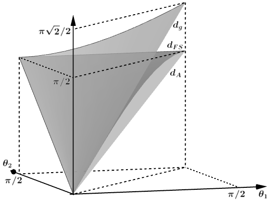
(a) angular metrics

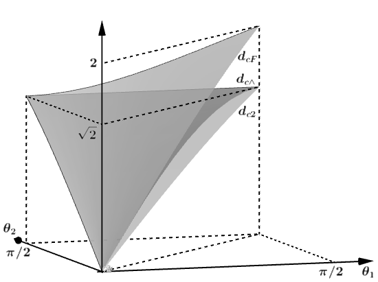
(b) chordal metrics

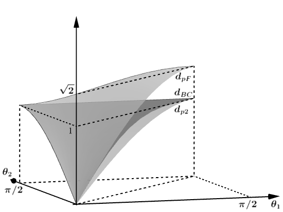
(c) gap metrics

Figure 7: Metrics in $G_{2}^{n}$ as functions of principal angles $\theta_{1}\leq\theta_{2}$

All these metrics are topologically equivalent, as the following inequalities show (Fig. 7). Note that distances decrease as one moves right (if $V\neq W$) or down (if $\dim(V\cap W)<p-1$) in Table 2.

Proposition B.1.

For distinct $V,W\in G_{p}^{n}$:

1. $\frac{\pi}{2}d_{pF}\geq d_{g}>d_{cF}>d_{pF}$.

2. $\frac{\pi}{2}d_{BC}\geq d_{FS}>d_{c\wedge}>d_{BC}$.

3. $\frac{\pi}{2}d_{p2}\geq d_{A}>d_{c2}>d_{p2}$.

Proof.

Follows from the formulas in Table 2, as for distinct lines $K$ and $L$ we have $\frac{\pi}{2}g_{K,L}\geq\theta_{K,L}>c_{K,L}>g_{K,L}$. ∎

Proposition B.2.

Let $V,W\in G_{p}^{n}$. The following inequalities hold if $\dim(V\cap W)<p-1$, and otherwise the strict $>$’s become $=$’s.

1. $\sqrt{p}\,d_{A}\geq d_{g}>d_{FS}>d_{A}$.

2. $\sqrt{p}\,d_{c2}\geq d_{cF}>d_{c\wedge}>d_{c2}$.

3. $\sqrt{p}\,d_{p2}\geq d_{pF}>d_{BC}>d_{p2}$.

Proof.

If $\dim(V\cap W)\geq p-1$ then $\theta_{i}=0$ for $i\neq p$, and the distance formulas give the equalities. For $\dim(V\cap W)<p-1$ we prove only the second inequality in each item, as the others are simple.

(i) We show $\cos^{-1}(\cos\theta_{1}\cdots\cos\theta_{p})\leq\sqrt{\theta_{1}^{2}+\cdots+\theta_{p}^{2}}$ for $\theta_{i}\in[0,\frac{\pi}{2}]$, with $<$ if $\theta_{p-1},\theta_{p}\neq 0$. For $p=2$, $f(x,y)=\cos^{-1}(\cos x\cos y)$, $g(x,y)=\sqrt{x^{2}+y^{2}}$ and $x,y\in\ (0,\frac{\pi}{2})$, it follows as $\frac{\partial g}{\partial x}=\frac{x}{\sqrt{x^{2}+y^{2}}}$ is increasing in $x$ and so $\frac{\partial g}{\partial x}>\frac{\sin x}{\sqrt{\sin^{2}x+\tan^{2}y}}=\frac{\partial f}{\partial x}$. Assuming it for some $p\geq 2$, let $x=\cos^{-1}(\cos\theta_{1}\cdots\cos\theta_{p})\leq\sqrt{\theta_{1}^{2}+\cdots+\theta_{p}^{2}}$, so $\cos^{-1}(\cos\theta_{1}\cdots\cos\theta_{p+1})=\cos^{-1}(\cos x\cos\theta_{p+1})\leq\sqrt{x^{2}+\theta_{p+1}^{2}}\leq\sqrt{\theta_{1}^{2}+\cdots+\theta_{p+1}^{2}}$, with the first inequality being $<$ if $\theta_{p},\theta_{p+1}\neq 0$.

(ii) $d_{c\wedge}=\sqrt{2-2\prod_{i=1}^{p}\cos\theta_{i}}$ and $d_{cF}=\sqrt{2p-2\sum_{i=1}^{p}\cos\theta_{i}}$, so we show $1-\prod_{i=1}^{p}x_{i}\leq p-\sum_{i=1}^{p}x_{i}$ for $x_{i}\in[0,1]$, with $<$ if $x_{p-1},x_{p}\neq 1$. For $p=2$ we have $1-x_{1}x_{2}\leq 1-x_{1}x_{2}+(1-x_{1})(1-x_{2})=2-x_{1}-x_{2}$, with $<$ if $x_{1},x_{2}\neq 1$. Assuming it for some $p\geq 2$, let $x=\prod_{i=1}^{p}x_{i}\geq 1-p+\sum_{i=1}^{p}x_{i}$. Then $1-\prod_{i=1}^{p+1}x_{i}=1-xx_{p+1}\leq 2-x-x_{p+1}\leq p+1-\sum_{i=1}^{p+1}x_{i}$, and the first inequality is $<$ if $x_{p},x_{p+1}\neq 1$.

(iii) As in ii, with $d_{pF}=\sqrt{p-\sum_{i=1}^{p}\cos^{2}\theta_{i}}$ and $x_{i}=\cos^{2}\theta_{i}$. ∎

Lastly, we note that the following are not metrics in $G_{p}^{n}$:

• The max-correlation or spectral distance [15, 12] $d=\sin\theta_{1}$ does not satisfy a triangle inequality, and $d=0\Leftrightarrow V\cap W\neq\{0\}$.

• The Martin metric for ARMA models [70] is given, for certain subspaces associated to the models [71], by $d=\sqrt{-\log\prod_{i=1}^{p}\cos^{2}\theta_{i}}$. It is presented in [21] as a metric for general subspaces, but does not satisfy a triangle inequality (e.g. take lines in $\mathds{R}^{2}$).

B.1 Fubini-Study metrics in $\mathds{P}(\mathds{F}^{n})$ and $G_{p}^{n}$

The Fubini-Study metric originates in the projective space $\mathds{P}(\mathds{F}^{n})=\{$lines of $\mathds{F}^{n}\}$, where it is just the angular distance, $d_{FS}(K,L)=\theta_{K,L}$. We prove its triangle inequality to obtain equality conditions.

Proposition B.3.

$\theta_{K,L}\leq\theta_{K,J}+\theta_{J,L}$ for $J,K,L\in\mathds{P}(\mathds{F}^{n})$, with equality if, and only if, $J=\operatorname{span}\{u\}$, $K=\operatorname{span}\{v\}$, $L=\operatorname{span}\{w\}$ for aligned $u,v,w\in\mathds{F}^{n}$ with $u=\kappa v+\lambda w$ for $\kappa,\lambda\geq 0$.

Proof.

Assume distinct lines and $\theta_{K,J}\neq\frac{\pi}{2}$. For a unit $v\in K$, let $u=\frac{P_{J}v}{\|P_{J}v\|}$. If $\theta_{K,L}\neq\frac{\pi}{2}$ let $w=\frac{P_{L}v}{\|P_{L}v\|}$, otherwise take a unit $w\in L$. Then $\theta_{K,J}=\theta_{u,v}$ and $\theta_{K,L}=\theta_{v,w}$. Let $u^{\perp}=\frac{u-P_{K}u}{\|u-P_{K}u\|}$ and $w^{\perp}=\frac{w-P_{K}w}{\|w-P_{K}w\|}$. As $P_{K}w=v\cos\theta_{v,w}$ and $\|w-P_{K}w\|=\sin\theta_{v,w}$, we find $w=v\cos\theta_{v,w}+w^{\perp}\sin\theta_{v,w}$. Likewise, $u=v\cos\theta_{u,v}+u^{\perp}\sin\theta_{u,v}$. So $\cos\theta_{J,L}=|\langle u,w\rangle|=|\cos\theta_{u,v}\cos\theta_{v,w}+\langle u^{\perp},w^{\perp}\rangle\sin\theta_{u,v}\sin\theta_{v,w}|\leq\cos(\theta_{v,w}-\theta_{u,v})$, and thus $\theta_{J,L}\geq\theta_{v,w}-\theta_{u,v}$.

Equality holds when $\theta_{v,w}>\theta_{u,v}$ and $\langle u^{\perp},w^{\perp}\rangle=1$, so $u^{\perp}=w^{\perp}$ and $u=v\cos\theta_{u,v}+\frac{w-P_{K}w}{\|w-P_{K}w\|}\sin\theta_{u,v}=v\frac{\sin(\theta_{v,w}-\theta_{u,v})}{\sin\theta_{v,w}}+w\frac{\sin\theta_{u,v}}{\sin\theta_{v,w}}=\kappa v+\lambda w$ with $\kappa,\lambda>0$. Conversely, if $u=\kappa v+\lambda w$ with $\kappa,\lambda\geq 0$ and $\langle v,w\rangle\geq 0$ then $\theta_{v,w}=\theta_{u,v}+\theta_{u,w}$ and, as $\langle u,v\rangle=\kappa\|v\|^{2}+\lambda\langle w,v\rangle\geq 0$ and likewise $\langle u,w\rangle\geq 0$, we have $\theta_{K,L}=\theta_{v,w}$, $\theta_{K,J}=\theta_{u,v}$ and $\theta_{J,L}=\theta_{u,w}$. ∎

The Plücker embedding $G^{n}\hookrightarrow\mathds{P}(\bigwedge\mathds{F}^{n})$ in the projective space of the Grassmann algebra maps $V\in G_{p}^{n}$ to its line $\bigwedge^{p}V$, and $G_{p}^{n}$ inherits the Fubini-Study metric $d_{FS}(V,W)=\theta_{\bigwedge^{p}V,\bigwedge^{p}W}=\theta_{e_{1}\wedge\cdots\wedge e_{p},f_{1}\wedge\cdots\wedge f_{p}}=\cos^{-1}(\prod_{i=1}^{p}\cos\theta_{i})$, where the $e_{i}$’s, $f_{i}$’s and $\theta_{i}$’s are principal vectors and angles. As the $\bigwedge^{p}\mathds{F}^{n}$’s are orthogonal, the $G_{p}^{n}$’s are separated by a distance of $\frac{\pi}{2}$, and $G^{n}$ has its usual disjoint union topology.

Lemma B.4.

Let $A,B,C\in\bigwedge^{p}\mathds{F}^{n}$ be nonzero blades with $[A],[B],[C]$ all distinct. If $A=\kappa B+\lambda C$ for $\kappa,\lambda\in\mathds{C}$, there are $u,v,w\in\mathds{F}^{n}$ and a unit blade $D\in\bigwedge^{p-1}\mathds{F}^{n}$ with $u=\kappa v+\lambda w$, $A=u\wedge D$, $B=v\wedge D$, $C=w\wedge D$ and $[D]=[A]\cap[B]\cap[C]$. We can choose $u$, $v$, $w$ in any complement of $[D]$, and if they are in $[D]^{\perp}$ then $\langle v,w\rangle=\langle B,C\rangle$.

Proof.

If $x\in[B]\cap[C]$ then $x\wedge A=x\wedge(\kappa B+\lambda C)=0$, so $x\in[A]$. As the spaces are distinct, $\kappa,\lambda\neq 0$, so $B$ and $C$ are also linear combinations of the other blades, and $[A]\cap[B]=[A]\cap[C]=[B]\cap[C]=[A]\cap[B]\cap[C]=[D]$ for a unit $q$-blade $D$. Given a complement $X$ of $[D]$, we have $A=A^{\prime}\wedge D$, $B=B^{\prime}\wedge D$ and $C=C^{\prime}\wedge D$ for blades $A^{\prime},B^{\prime},C^{\prime}\in\bigwedge^{p-q}X$ with $[A^{\prime}]$, $[B^{\prime}]$ and $[C^{\prime}]$ all disjoint. As $(A^{\prime}-\kappa B^{\prime}-\lambda C^{\prime})\wedge D=0$ and $A^{\prime}-\kappa B^{\prime}-\lambda C^{\prime}\in\bigwedge X$, Proposition A.1 gives $A^{\prime}=\kappa B^{\prime}+\lambda C^{\prime}$. For any nonzero $v^{\prime}\in[B^{\prime}]$ and $w^{\prime}\in[C^{\prime}]$ we have $A^{\prime}\wedge v^{\prime}\wedge w^{\prime}=0$, and as $A^{\prime}\wedge v^{\prime}\neq 0$ (by Proposition A.1) this means $w^{\prime}\in[A^{\prime}\wedge v^{\prime}]=[A^{\prime}]\oplus[v^{\prime}]$. Since $w^{\prime}\not\in[A^{\prime}]$ and $v^{\prime}$ was chosen at will in $[B^{\prime}]$, this implies $\dim[B^{\prime}]=1$. Thus $A^{\prime},B^{\prime},C^{\prime}$ are vectors $u,v,w$. If $X=[D]^{\perp}$ then $\langle B,C\rangle=\langle v\wedge D,w\wedge D\rangle=\langle v,w\rangle\cdot\|D\|^{2}$. ∎

Proposition B.5 (​[65]).

For distinct $U,V,W\in G_{p}^{n}$, we have $d_{FS}(V,W)=d_{FS}(V,U)+d_{FS}(U,W)\Leftrightarrow U=[u]\oplus R$, $V=[v]\oplus R$ and $W=[w]\oplus R$ for $R\in G_{p-1}^{n}$ and aligned $u,v,w\in R^{\perp}$ with $u=\kappa v+\lambda w$ for $\kappa,\lambda>0$.

Proof.

($\Rightarrow$) Proposition B.3, in $\mathds{P}(\bigwedge^{p}\mathds{F}^{n})$, gives $U=[A]$, $V=[B]$ and $W=[C]$ for aligned blades with $A=\kappa B+\lambda C$ for $\kappa,\lambda>0$ (strict as $U\neq V$ or $W$). Lemma B.4 gives the result, for $R=[D]$. ($\Leftarrow$) Immediate. ∎

Corollary B.6.

For distinct $V,W\in G_{p}^{n}$, the following are equivalent:

1. $\dim(V\cap W)=p-1$.

2. There is a segment from $V$ to $W$ for $d_{FS}$.

3. There is a distinct point between $V$ and $W$ for $d_{FS}$.

Proof.

(i$\,\Leftrightarrow\,$ii) By Proposition B.2. (i$\,\Leftrightarrow\,$iii) By Proposition B.5. ∎

Corollary B.7.

$G_{p}^{n}$ is convex for $d_{FS}\Leftrightarrow$ $p\in\{0,1,n-1,n\}$.

This corrects [65, Thm. 6].

References

- [1] S. Kobayashi and K. Nomizu. Foundations of Differential Geometry, volume 2. Wiley, 1996.
- [2] S. E. Kozlov. Geometry of real Grassmann manifolds. Parts I, II. J. Math. Sci., 100(3):2239–2253, 2000.
- [3] S. E. Kozlov. Geometry of real Grassmann manifolds. Part III. J. Math. Sci., 100(3):2254–2268, 2000.
- [4] Y. Wong. Differential geometry of Grassmann manifolds. Proc. Natl. Acad. Sci. USA, 57(3):589–594, 1967.
- [5] L. Qiu, Y. Zhang, and C. Li. Unitarily invariant metrics on the Grassmann space. SIAM J. Matrix Anal. Appl., 27(2):507–531, 2005.
- [6] A. Edelman, T. A. Arias, and S. T. Smith. The geometry of algorithms with orthogonality constraints. SIAM J. Matrix Anal. Appl., 20(2):303–353, 1999.
- [7] G. Stewart and J. Sun. Matrix Perturbation Theory. Academic Press, 1990.
- [8] T. Kato. Perturbation Theory for Linear Operators. Springer, 1995.
- [9] L. Zheng and D. N. C. Tse. Communication on the Grassmann manifold: a geometric approach to the noncoherent multiple-antenna channel. IEEE Trans. Inform. Theory, 48(2):359–383, 2002.
- [10] D. J. Love, R. W. Heath, and T. Strohmer. Grassmannian beamforming for multiple-input multiple-output wireless systems. IEEE Trans. Inform. Theory, 49(10):2735–2747, 2003.
- [11] D. J. Love and R. W. Heath. Limited feedback unitary precoding for orthogonal space-time block codes. IEEE Trans. Signal Process., 53(1):64–73, 2005.
- [12] I. S. Dhillon, R. W. Heath Jr., T. Strohmer, and J. A. Tropp. Constructing packings in Grassmannian manifolds via alternating projection. Exp. Math., 17(1):9–35, 2008.
- [13] J. H. Conway, R. H. Hardin, and N. J. A. Sloane. Packing lines, planes, etc.: Packings in Grassmannian spaces. Exp. Math., 5(2):139–159, 1996.
- [14] A. Barg and D. Y. Nogin. Bounds on packings of spheres in the Grassmann manifold. IEEE Trans. Inform. Theory, 48(9):2450–2454, 2002.
- [15] J. Hamm and D. Lee. Grassmann discriminant analysis: A unifying view on subspace-based learning. In Proc. Int. Conf. Mach. Learn., pages 376–383. ACM, 2008.
- [16] Z. Huang, J. Wu, and L. Van Gool. Building deep networks on Grassmann manifolds. In Proc. Conf. AAAI Artif. Intell., volume 32, 2018.
- [17] G. Lerman and T. Zhang. Robust recovery of multiple subspaces by geometric minimization. Ann. Stat., 39(5):2686–2715, 2011.
- [18] Y. M. Lui. Advances in matrix manifolds for computer vision. Image Vis. Comput., 30(6-7):380–388, 2012.
- [19] P. Turaga, A. Veeraraghavan, and R. Chellappa. Statistical analysis on Stiefel and Grassmann manifolds with applications in computer vision. In 2008 IEEE Conf. Comput. Vis. Pattern Recog., 2008.
- [20] S. V. N. Vishwanathan, A. J. Smola, and R. Vidal. Binet-Cauchy kernels on dynamical systems and its application to the analysis of dynamic scenes. Int. J. Comput. Vis., 73(1):95–119, 2006.
- [21] K. Ye and L. H. Lim. Schubert varieties and distances between subspaces of different dimensions. SIAM J. Matrix Anal. Appl., 37(3):1176–1197, 2016.
- [22] R. Basri, T. Hassner, and L. Zelnik-Manor. Approximate nearest subspace search. IEEE Trans. Pattern Anal. Mach. Intell., 33(2):266–278, 2011.
- [23] B. Draper, M. Kirby, J. Marks, T. Marrinan, and C. Peterson. A flag representation for finite collections of subspaces of mixed dimensions. Linear Algebra Appl., 451:15–32, 2014.
- [24] R. Pereira, X. Mestre, and D. Gregoratti. Subspace based hierarchical channel clustering in massive MIMO. In 2021 IEEE Globecom Workshops, pages 1–6, 2021.
- [25] P. Gruber, H. W. Gutch, and F. J. Theis. Hierarchical extraction of independent subspaces of unknown dimensions. In Int. Conf. Ind. Compon. Anal. Signal Separation, pages 259–266. Springer, 2009.
- [26] E. Renard, K. A. Gallivan, and P. A. Absil. A Grassmannian minimum enclosing ball approach for common subspace extraction. In Int. Conf. Latent Variable Anal. Signal Separation, pages 69–78, 2018.
- [27] C. A. Beattie, M. Embree, and D. C. Sorensen. Convergence of polynomial restart Krylov methods for eigenvalue computations. SIAM Review, 47(3):492–515, 2005.
- [28] D. C. Sorensen. Numerical methods for large eigenvalue problems. Acta Numer., 11:519–584, 2002.
- [29] L. Wang, X. Wang, and J. Feng. Subspace distance analysis with application to adaptive Bayesian algorithm for face recognition. Pattern Recognit., 39(3):456–464, 2006.
- [30] X. Sun, L. Wang, and J. Feng. Further results on the subspace distance. Pattern Recognit., 40(1):328–329, 2007.
- [31] W. A. Wilson. On quasi-metric spaces. Amer. J. Math., 53(3):675, 1931.
- [32] H. Busemann. Local metric geometry. Trans. Amer. Math. Soc., 56:200–274, 1944.
- [33] E. M. Zaustinsky. Spaces with non-symmetric distance, volume 34. American Mathematical Soc., 1959.
- [34] G. E. Albert. A note on quasi-metric spaces. Bull. Amer. Math. Soc., 47(6):479–482, 1941.
- [35] A. C. G. Mennucci. On asymmetric distances. Anal. Geom. Metr. Spaces, 1(1):200–231, 2013.
- [36] J. Goubault-Larrecq. Non-Hausdorff Topology and Domain Theory. Cambridge University Press, 2013.
- [37] H. P. Künzi. Nonsymmetric distances and their associated topologies: about the origins of basic ideas in the area of asymmetric topology. In C. E. Aull and R. Lowen, editors, Handbook of the history of general topology, volume 3, pages 853–968. Springer, 2001.
- [38] H. P. Künzi. An introduction to quasi-uniform spaces. Contemp. Math., 486:239–304, 2009.
- [39] D. Bao, S. S. Chern, and Z. Shen. Introduction to Riemann-Finsler Geometry. Springer, 2012.
- [40] G. Gutierres and D. Hofmann. Approaching metric domains. Appl. Categ. Structures, 21(6):617–650, 2012.
- [41] F. W. Lawvere. Metric spaces, generalized logic, and closed categories. Rend. Sem. Mat. Fis. Milano, 43(1):135–166, 1973. Reissued in Reprints in Theory and Applications of Categories 1 (2002), 1–37.
- [42] G. Mayor and O. Valero. Aggregation of asymmetric distances in computer science. Inform. Sci., 180(6):803–812, 2010.
- [43] S. Romaguera and M. Schellekens. Quasi-metric properties of complexity spaces. Topol. Appl., 98(1-3):311–322, 1999.
- [44] A. K. Seda and P. Hitzler. Generalized distance functions in the theory of computation. Comput. J., 53(4):443–464, 2008.
- [45] Y. Fang. Asymmetrically weighted graphs, asymmetric metrics and large scale geometry. Geom. Dedicata, 217(2), 2022.
- [46] A. Stojmirović. Quasi-metric spaces with measure. Topol. Proc., 28(2):655–671, 2004.
- [47] R. Kopperman. Asymmetry and duality in topology. Topol. Appl., 66(1):1–39, 1995.
- [48] J. C. Kelly. Bitopological spaces. Proc. Lond. Math. Soc., s3-13(1):71–89, 1963.
- [49] I. V. Chenchiah, M. O. Rieger, and J. Zimmer. Gradient flows in asymmetric metric spaces. Nonlinear Anal. Theory Methods Appl., 71(11):5820–5834, 2009.
- [50] J. Collins and J. Zimmer. An asymmetric Arzelà–Ascoli theorem. Topol. Appl., 154(11):2312–2322, 2007.
- [51] S. Cobzas. Functional Analysis in Asymmetric Normed Spaces. Springer, 2012.
- [52] L. M. García-Raffi, S. Romaguera, and E. A. Sanchez-Pérez. The dual space of an asymmetric normed linear space. Quaest. Math., 26(1):83–96, 2003.
- [53] S. Romaguera and P. Tirado. A characterization of Smyth complete quasi-metric spaces via Caristi’s fixed point theorem. Fixed Point Theory Appl., 2015(1):1–13, 2015.
- [54] A. C. G. Mennucci. Geodesics in asymmetric metric spaces. Anal. Geom. Metr. Spaces, 2(1):115–153, 2014.
- [55] I. Bengtsson and K. Życzkowski. Geometry of quantum states: an introduction to quantum entanglement. Cambridge University Press, 2017.
- [56] A. L. G. Mandolesi. Grassmann angles between real or complex subspaces. arXiv:1910.00147, 2019.
- [57] A. L. G. Mandolesi. Blade products and angles between subspaces. Adv. Appl. Clifford Algebras, 31(69), 2021.
- [58] A. Rosén. Geometric Multivector Analysis. Springer-Verlag, 2019.
- [59] A. L. G. Mandolesi. Asymmetric trigonometry of subspaces. Manuscript in preparation.
- [60] A. L. G. Mandolesi. Projection factors and generalized real and complex Pythagorean theorems. Adv. Appl. Clifford Algebras, 30(43), 2020.
- [61] A. L. G. Mandolesi. Quantum fractionalism: the Born rule as a consequence of the complex Pythagorean theorem. Phys. Lett. A, 384(28):126725, 2020.
- [62] A. Bjorck and G. Golub. Numerical methods for computing angles between linear subspaces. Math. Comp., 27(123):579, 1973.
- [63] B. Bajnok. An Invitation to Abstract Mathematics. Springer, 2nd edition, 2020.
- [64] J. A. Wolf. Spaces of constant curvature. AMS Chelsea Pub., 2011.
- [65] S. Jiang. Angles between Euclidean subspaces. Geom. Dedicata, 63:113–121, 1996.
- [66] M. A. Schlosshauer. Decoherence and the quantum-to-classical transition. Springer, 2007.
- [67] A. L. G. Mandolesi. A review of multivector contractions, part I. arXiv:2205.07608 [math.GM], 2022.
- [68] D. Asimov. The grand tour: A tool for viewing multidimensional data. SIAM J. Sci. Stat. Comp., 6(1):128–143, 1985.
- [69] A. Weinstein. Almost invariant submanifolds for compact group actions. J. Eur. Math. Soc., 2(1):53–86, 2000.
- [70] R. J. Martin. A metric for ARMA processes. IEEE Trans. Signal Process., 48(4):1164–1170, 2000.
- [71] K. De Cock and B. De Moor. Subspace angles between ARMA models. Syst. Control Lett., 46(4):265–270, 2002.