Boosting Data Analytics with Synthetic Volume Expansion
Abstract
Synthetic data generation, a cornerstone of Generative Artificial Intelligence (GAI), signifies a paradigm shift in data science by addressing data scarcity and privacy while enabling unprecedented performance. As synthetic data gains prominence, questions arise concerning the accuracy of statistical methods when applied to synthetic data compared to raw data. This article introduces the Synthetic Data Generation for Analytics (Syn) framework. This framework employs statistical methods on high-fidelity synthetic data generated by advanced models such as tabular diffusion and Generative Pre-trained Transformer (GPT) models. These models, trained on raw data, are further enhanced with insights from pertinent studies through knowledge transfer. A significant discovery within this framework is the generational effect: the error of a statistical method on synthetic data initially diminishes with additional synthetic data but may eventually increase or plateau. This phenomenon, rooted in the complexities of replicating raw data distributions, highlights a “reflection point” — an optimal threshold in the size of synthetic data determined by specific error metrics. Through three case studies — sentiment analysis of texts, predictive modeling of structured data, and inference in tabular data — we demonstrate the effectiveness of this framework over traditional ones. We underline its potential to amplify various statistical methods, including gradient boosting for prediction and hypothesis testing, thereby underscoring the transformative potential of synthetic data generation in data science.
keywords:
, and
1 Introduction
The advent of synthetic data generation, fueled by generative artificial intelligence (AI), has shifted data analytics towards a more synthetic data-centric approach. According to Gartner, 60% of the data utilized in AI and analytics projects will be synthetically generated by 2024, and synthetic data will surpass real data in AI models by 2030 (Gartner, 2022; Eastwood, 2023). This paradigm shift challenges the traditional practice, which exclusively relies on raw data. Synthetic data, mirroring real-world scenarios, presents a viable alternative to the challenges posed by data collection, sharing, and analysis within limited data environments.
Synthetic data confers two primary advantages on data analytics (Walonoski et al., 2018; Topol, 2019). First, it alleviates data scarcity and addresses privacy concerns (Ghalebikesabi et al., 2023). When crafted to emulate the raw data distribution (Bi and Shen, 2023; Shen, Bi and Shen, 2022; Xie et al., 2018), sharing synthetic data comes with minimal risk of exposing sensitive raw data. The significance of such data is accentuated in downstream or subsequent analyses, as exemplified by a COVID-19 study (El Emam et al., 2021). Second, synthetic data enables training in real-world scenarios like autonomous driving (Sun et al., 2020; Liu, Shen and Shen, 2023), negating the necessity for expensive experiments. Moreover, it proves invaluable for approximating the distributions of test statistics using Monte Carlo methods through repeated numerical experiments (Liu, Shen and Shen, 2023).
This paper introduces the Synthetic Data Generation for Analytics (Syn) framework, designed to bolster the precision of any statistical methods using high-fidelity synthetic data that closely mirrors raw data, thereby harnessing the anticipated advantages. Generative models produce synthetic data by training on raw data and enrichment with insights from related studies via knowledge transfer. The Syn framework employs an array of generative models suited for various domains: image diffusion (Sohl-Dickstein et al., 2015; Wei et al., 2021), text diffusion models (Ho, Jain and Abbeel, 2020), text-to-image diffusion models (Zhang et al., 2023), time-series diffusion models (Lin et al., 2023), spatio-temporal diffusion models (Yuan et al., 2023), and tabular diffusion models (Kotelnikov et al., 2023; Zheng and Charoenphakdee, 2022; Kim, Lee and Park, 2022; Lee, Kim and Park, 2023). Moreover, Syn embraces advanced models such as the Reversible Generative Models (Kingma and Dhariwal, 2018). These flow-based models capture the raw data distribution and can estimate both conditional and marginal distributions. Central to our Syn exploration is this pivotal issue: Can high-fidelity synthetic data enhance the efficacy of statistical methods solely reliant on raw data? If so, how may we implement such enhancements? Recent research offers diverging viewpoints on this issue. In some cases, synthetic X-ray images improve the accuracy of machine learning models (Gao et al., 2023), whereas, in others, training on synthetic data may compromise performance for some machine learning models (Kotelnikov et al., 2023).
Synthetic data holds immense potential for enhancing data analytics. When generated accurately, this high-fidelity data can boost the accuracy of a statistical method by expanding the sample size of raw data. However, a significant caveat exists: low-fidelity synthetic data could yield unreliable outcomes. Often, a generational effect emerges, whereby as the size of synthetic data grows, the precision gain might diminish or even plateau. This phenomenon has been exemplified in our case study focusing on structured data prediction as discussed in Section 4.2. This challenge arises from generation errors or discrepancies between the data-generation distributions of synthetic and raw data. Fundamentally, the generational effect underscores a key concern: regardless of the size of synthetic data, generation errors can compromise the accuracy of a statistical method.
While evaluating predictive tasks is typically straightforward, hypothesis testing presents the challenge of regulating the Type-I error. To address this challenge and enhance the power of a test, we introduce “Syn-Test,” a test that augments the sample size of raw data by applying synthetic data. For clarity, “Syn-A” denotes Method A within the Syn framework throughout this article. Syn-Test determines the ideal size of synthetic data required to manage the empirical Type-I error while performing a test for finite inference samples using Monte Carlo methods. Our research indicates that the ideal size of synthetic data can heighten the accuracy. Moreover, our theoretical investigation sheds light on the generational effect, precision, and the size of synthetic data.
Additionally, we introduce a streamlined approach called Syn-Slm to improve Syn’s usability in applications. This approach forgoes actual data generation when one knows the synthetic data distribution. Using sentiment analysis as an illustration, we demonstrate that Syn-Slm is competitive with some alternatives under the Syn framework.
To showcase the capabilities of the Syn framework, we delve into three key domains: sentiment analysis of texts, predictive modeling for structured data, and inference on tabular data. Across these domains, all statistical methods leveraging high-fidelity synthetic data surpass their counterparts employing raw data. The superior performance is due to high-fidelity synthetic data generated by diffusion models. Initially trained on raw data, these models are further improved by fine-tuning pre-trained models via knowledge transfer, resulting in enhanced statistical accuracy and larger sample sizes.
In the first area, we contrasted three models: OpenAI’s Generative Pre-trained Transformer (GPT)-3.5 within the Syn framework, Distilling BERT (DistilBERT, Sanh et al. (2019)) in the Syn-Slm framework, and the Long Short-term Memory Networks (LSTM) in the traditional framework for analyzing consumer reviews from the IMDB movie dataset. In this context, Syn’s generative capability using GPT-3.5 significantly outperforms the LSTM approach. Yet, the Syn-Slm framework using DistilBERT, although trailing, demonstrated notable competitiveness compared to GPT-3.5.
In the second area, we introduced Syn-Boost, a version of CatBoost (Dorogush, Ershov and Gulin, 2018)—a gradient boosting algorithm (Schapire, 1990)—trained on synthetic data. Syn-Boost bolsters the precision of CatBoost for both regression and classification tasks across eight real-world datasets, utilizing a refined tabular diffusion model (Kotelnikov et al., 2023). Statistically, the error trajectory of Syn-Boost exhibits either a U-shaped or L-shaped pattern, determined by the generation errors and the volume of synthetic data used. Moreover, when employing the same knowledge transfer methods, Syn-Boost surpasses traditional feed-forward networks trained on raw data in six of eight cases. These observations highlight that the generative approach of Syn offers a predictive advantage even against a top predictive methodology given the same data input.
In the third domain, we explore the pivotal role of significance tests in discerning feature relevance in regression and classification using CatBoost. This exploration within black-box models unveils largely uncharted territory. Recently, Dai, Shen and Pan (2022) introduced a nonparametric asymptotic test through sample splitting. To augment its statistical prowess, we employ the Syn-Test, capitalizing on pre-trained generative models and knowledge transfer, as demonstrated in two distinct scenarios. In one scenario, we leverage a pre-trained model to ensure smooth knowledge transfer from the male data to the female data while improving generation fidelity and test accuracy for female data, especially when male and female data distributions present distinct characteristics. These observations emphasize the importance of knowledge transfer in mitigating disparities in domains such as healthcare and social science, particularly when data for specific subgroups, like minorities, are limited. Moreover, we shed light on the “generational effect”, accentuating the invaluable interplay of synthetic data generation and knowledge transfer in hypothesis testing—a domain rarely explored in current literature.
This article consists of six sections. Section 2 explores Syn’s role in enhancing the accuracy of statistical methods and emphasizes the importance of knowledge transfer in synthetic data generation. Section 3 discusses the streamlined approach—Syn-Slm and its impact on generative techniques in statistical practice. Section 4 provides illustrative examples, exploring the generational effect in predictive modeling and inference. Section 5 focuses on the privacy issue of synthetic data. In Section 6, we discuss the implications of generating synthetic data for data science. The Appendix contains technical details.
2 Enhancing Statistical Accuracy
2.1 Synthetic Data
The Syn framework empowers data analytics by applying statistical methods on a synthetic sample . This sample is generated by a generative model trained on raw data through fine-tuning a pre-trained model, leveraging insights from various similar studies. These models include GPT (Brown et al., 2020; Bubeck et al., 2023; OpenAI, 2023), diffusion models (Ho, Jain and Abbeel, 2020; Song, Meng and Ermon, 2020), normalizing flows (Dinh, Krueger and Bengio, 2014; Dinh, Sohl-Dickstein and Bengio, 2016; Kingma and Dhariwal, 2018), and GANs (Frid-Adar et al., 2018; Liu et al., 2020). For an in-depth understanding of the generation processes for diffusion models and flows, readers refer to (Liu, Shen and Shen, 2023). In this framework, the cumulative distribution function (CDF) of estimates the CDF of . To produce high-fidelity synthetic data, fine-tuning a pre-trained generative model is recommended, which involves transferring knowledge from previous studies. If pre-trained models are unsuitable, constructing a generative model from scratch is a viable, though less preferred, alternative. The quality of the generated data hinges on the choice of generative model and the effectiveness of knowledge transfer from similar studies. For an illustration, we detail the synthetic data generation process using a diffusion model in Figure 1. Furthermore, to demonstrate the importance of knowledge transfer, we fine-tune a pre-trained tabular diffusion model (Shwartz-Ziv and Armon, 2022) on the Adult-Male dataset to apply this knowledge to the Adult-Female dataset in Section 4.3, where male and female distributions exhibit distinct differences. For a detailed explanation of the impact of knowledge transfer, readers refer to Section 2.4.
It is imperative to underscore the pivotal role of knowledge encapsulated in pre-trained generative models for improving generation accuracy through fine-tuning. Nevertheless, directly accessing the pre-training data for pre-trained models is frequently infeasible, impeded by privacy concerns, extensive storage needs, and data inconsistencies (Sweeney, 2002; Quionero-Candela et al., 2009; Labrinidis and Jagadish, 2012; Carroll, 2006), as seen in models like GPT-4. Furthermore, the distributions of pre-training datasets, especially from different sources, might not always mirror that of raw data, as illustrated by the Adult-Male and Adult-Female examples in Section 4.3. Considering these challenges and the nuances of real-world scenarios, we omit pre-training data from our raw data composition throughout this article.
To yield directly, one can utilize some revertible generative models such as normalizing flows and Roundtrip GAN (Liu et al., 2020), acting as a nonparametric estimate of . For other generative models, such as diffusion models and GPT, one can typically obtain from synthetic data employing Monte Carlo methods, which we elaborate on in Section 3. In the numerical examples presented in this paper, we utilize a tabular diffusion model TDM (Kotelnikov et al., 2023) and GPT for synthetic data generation.
Subsequently, we explore the precision advantages offered by the Syn framework.
2.2 Optimal Synthetic Size for Estimation and Prediction
In estimation and prediction, leveraging a statistical method on a synthetic sample gives rise to an estimate, denoted as , of a parameter vector . The effectiveness of this method gauges through a specific error metric , which would theoretically improve the statistical accuracy of with an infinite amount of synthetic data, provided perfectly replicates . Here, symbolizes the expectation under , while represents a loss function quantifying the discrepancies between and . However, numerical insights from Section 4.2 reveal the existence of a reflection point, denoted as , which delineates a relationship between the synthetic sample size and the accuracy augmentation for this method. This point is governed by the generation error measured by metrics such as the total variation distance between and , defined as , where and are probabilities measures induced by and and is any event.
To estimate , we optimize its empirical risk measure across on an independent cross-validation sample from the original resources, which yields an optimizer as an estimate of . For instance, in scenarios where the risk measure is the generalization error in binary classification, its empirical risk is the test error on a test dataset obtained from the original resources, approximating a classifier’s generalizability.
To investigate the theoretical aspects of the generational effect concerning the accuracy of , we clarify the notation: Let represent the discrepancy between the synthetic and raw errors for a sample size , where denotes the risk incurred when employing a raw sample of size .
Theorem 2.1 (Reflection Point).
Suppose can be expressed as for some constant . Moreover, assume that if and if for some finite index , where LTV is the learning error induced by the generation error. Then, the minimum of occurs at a finite provided that LTV is larger than .
As stated in Theorem 2.1, a sizable generation error leads to the synthetic risk minimizing at a finite , after which the synthetic error starts to deteriorate. This result suggests that augmented synthetic sample size may not enhance estimation or prediction given substantial generation error, a phenomenon further exemplified in Section 4.2. Conversely, with a small generation error, the synthetic risk remains controlled, and the optimal tends to be significantly large or infinite, as substantiated by Theorem 2.2.
Next, we establish a bound on the synthetic risk to offer insight into the conditions under which accuracy improvements may arise. Assume that is independently and identically distributed according to while is independently and identically distributed according to a conditional distribution given .
Theorem 2.2 (Accuracy Gain).
Let be a nonnegative loss function upper-bounded by . For any ,
| (1) |
Moreover, if , then
| (2) |
when . Hence, achieves an accuracy gain under Syn when the total variation is sufficiently small. For example, this occurs when .
Theorem 2.2 posits that training a method trained on synthetic data can lead to an accuracy gain, provided that the generation error that governs the synthetic risk is small. Hence, high-fidelity data can mitigate the synthetic risk in a method, thereby enabling a large optimal synthetic size for further amplifying the precision.
The existing literature provides insights into the magnitude of generation error as represented by . For instance, Theorem 5.1 in Oko, Akiyama and Suzuki (2023) specifies bounds for a diffusion model, given the data-generating distribution is a member of a Besov space. It’s worth noting that the boundary defined in Oko, Akiyama and Suzuki (2023) pertains to , with symbolizing the expectation relative to . However, one may extend this to the in-probability convergence rate for the random quantity by leveraging Markov’s inequality, which provides the convergence rates for based on the raw sample size and/or the pre-training sample size.
2.3 Optimal Synthetic Size for Hypothesis Testing
We now introduce Syn-Test, a novel inference tool using high-fidelity synthetic data to boost any test’s power by expanding the sample size of raw data. Syn-Test yields two distinct advantages. First, it employs synthetic data to gauge the null distribution of any test statistic by Monte Carlo methods as in the bootstrap approach (Efron, 1992), circumventing analytical derivations. This methodology proves particularly powerful for unstructured data inferences, including texts and images (Liu, Shen and Shen, 2023). Second, Syn-Test identifies the optimal synthetic data size, optimizing a test’s power while maintaining a suitable control of Type-I errors. For illustration, we refer to Section 4.3.
Given a raw sample, Syn-Test employs two nearly equal-sized subsamples and , partitioned from a training sample for fine-tuning a pre-trained generative model. It also uses a separate inference sample of size for validating model training. One generative model generates synthetic data using for null distribution estimation, while the other uses for computing the test statistic. Figure 4 illustrates the splitting scheme and Syn-Test process. Syn-Test also empirically determines the optimal synthetic data size to control the Type-I error. By swapping the roles of and , Syn-Test can de-randomize the partition, transitioning the original inference sample size to a synthetic inference sample size of . This swapping mechanism proves especially advantageous in scenarios with low generation error. Crucially, abundant synthetic data can enhance the size of the raw data, even when sample splitting results in a reduced inference sample size (Wasserman and Roeder, 2009; Wasserman, Ramdas and Balakrishnan, 2020).
Syn-Test encompasses four steps, using a significance level , a tolerance error , and a Monte Carlo size . Syn-Test goes as follows:
Step 1: Controlling Type-I Error. Generate distinct synthetic samples of size by refining a pre-trained generative model with under . Compute the empirical distribution of the test statistic using . Define a rejection region at a significance level where .
Step 2: Optimizing Synthetic Size through Tuning. Execute Step 1, but use instead of to produce . Utilize the empirical distribution from to find the empirical Type-I error, denoted , for the created in Step 1. To effectively control the Type-I error, we propose two distinct strategies for identifying : an aggressive and a conservative approach. The aggressive approach selects the largest that maintains the estimated Type-I error within the desired limit. In contrast, the conservative one chooses the smallest about failing to control the estimated Type-I error. Mathematically,
-
1.
Aggressive: .
-
2.
Conservative: .
In practice, we recommend adopting a conservative approach, as it more effectively manages Type-I errors, although it may be less powerful compared to a more aggressive strategy.
Step 3: Calculating the P-value. With the determined , produce synthetic data by fine-tuning the pre-trained generative model using . Calculate the test statistic for and determine the P-value, , leveraging the null CDF based on .
Step 4: Combining the P-values. Repeat Step 3 by interchanging the roles of and to compute the P-value . Combine P-values via Hommel’s weighted average (Hommel, 1983):
where and is the -th order statistic of .
Hommel’s method excels in controlling the Type-I error relative to many of its peers, ensuring that under . While effective, there are also alternative strategies such as the Cauchy combination (Liu and Xie, 2020). To expedite the search of an estimated , we may consider techniques such as Bisection (Burden and Faires, 2001) or Fibonacci Search (Kiefer, 1953).
Theorem 2.3 (Validity and power of Syn-Test).
Assume that is an i.i.d. sample of size following given . Let and be the synthetic and raw distributions of calculated on a sample of size . Then, the estimation error of the null distribution is governed by the Monte Carlo error and the generation error:
| (3) |
As a result, Syn-Test offers a valid test as long as in probability and . Moreover, let the power function be for rejection region at significance level , and analogously with . If for some , , then when , indicating that Syn-Test enhances power if the generation error is small.
Syn-Test enables valid inference without requiring many model assumptions, specific data distributions, and an infinitely large inference sample. Instead, its validity and power hinge on the generation error, which is generally satisfied when using generative models trained on adequately large datasets.
Syn-Test is adept at debiasing test statistics. In this context, the bias estimation is achieved through a Monte Carlo (MC) approach, utilizing synthetic samples generated by a refined generative model. This estimated bias is then subtracted from the estimated null distribution, leading to a debiased version of the test statistic. The effectiveness of this aspect of Syn-Test is demonstrated through numerical examples, as detailed in Section 4.3.
2.4 Generative Model and Knowledge Transfer
Knowledge transfer elevates generation accuracy by infusing task-specific generative models with pre-trained knowledge from relevant studies. From the perspective of dimension reduction, we dissect knowledge transfer in two scenarios. In the first situation, consider a generative model parametrized by . Originally trained on an extensive dataset for a generation task, the model undergoes subsequent fine-tuning on a smaller but similar dataset to account for distribution shift, resulting in model , where the architecture remains consistent across both models, with the essence of knowledge transmission occurring via the transition from to amid the fine-tuning. In the other situation, a robust pre-trained model undergoes training across multiple tasks, characterized as . Here, defines the output function tied to the -th task, is the shared representation function, and denotes functional composition. Given a learned representation , one only fine-tune during its optimization phase for (Tripuraneni, Jordan and Jin, 2020). As the generative model refines its precursor, it absorbs the precisely calibrated representation . This knowledge transfer thus can augment the generation precision through fine-tuning with a heightened accuracy of the learned , facilitating its dimension reduction. It is pivotal to acknowledge that within this configuration, and ; , only share the same architecture in . An alternate strategy entails concurrent fine-tuning of and to derive a representation explicitly for .
The Syn framework capitalizes on knowledge transfer to bolster its overall efficacy, streamlining the synthetic data generation process. In Section 4.3, we illustrate knowledge transfer in generative models using a pre-trained model based on adult male data (Kohavi et al., 1996), subsequently fine-tuned with adult female data for downstream analysis. As demonstrated in Figures 6, 7, and Table 3, the fine-tuned model adeptly captures the data distribution, even with a limited size of raw samples.
3 Syn-Slm: Streamlined Approach
The Syn Framework enables unsupervised synthetic data generation, mirroring raw data distributions. It is adept at tackling statistical challenges in both unsupervised and supervised realms. It can also derive directly from some generative models such as normalizing flows (Kingma and Dhariwal, 2018). Subsequently, we will explore a streamlined method, termed Syn-Slm, which bypasses synthetic data generation.
3.1 Synthetic Data Distribution
The synthetic data distribution may degenerate when supported on a low-dimensional manifold, particularly if some components of exhibit functional dependence. Accessing can be challenging, even when it is non-degenerate, especially for some generative models. However, when we derive from a generative model, it becomes a nonparametric estimate of the raw data distribution . For a parameter of interest, expressed as , our streamlined method Syn-Slm gives rise to a plug-in estimate . As an example, if denotes the mean, then , yielding the Syn-Slm estimate . Section 4.1 illustrates this method.
3.2 Statistical Methodologies
Supervised learning aims to predict an outcome based on a predictor vector . Consider a one-dimensional outcome variable and define . In this scenario, generative models, such as diffusion models (Sohl-Dickstein et al., 2015; Ho, Jain and Abbeel, 2020) and the Reversible Generative Models (Kingma and Dhariwal, 2018), not only can generate synthetic data conditioning on but also provide the conditional CDF of synthetic data as an estimate of the conditional cumulative distribution function (CDF) . From this, one can deduce an optimal prediction function by minimizing the expected loss: . Here, symbolizes a loss function. For instance, if is the - loss in binary classification, then , and its Syn-Slm estimate is given by . An example is available in Section 4.1.
4 Case Studies
4.1 Sentiment Analysis
This subsection presents sentiment classification applied to the benchmark dataset, IMDB (Maas et al., 2011). This task involves assigning emotions expressed in the text into positive or negative sentiments based on the opinions reflected in each text. The dataset comprises polarized movie reviews, categorized as “positive” or “negative” sentiments. These labels correspond to movie scores below four or above seven out of ten, where no movie has more than 30 reviews to prevent significant class imbalance. Here, we use of these reviews as our training data, reserving reviews for testing. We compare Syn’s generative approach against its conventional counterpart in a downstream prediction task, utilizing three state-of-the-art models, GPT-3.5, DistilBERT, and LSTM models (Chen et al., 2023).
GPT-3.5 functions primarily as a text completion model, predicting the succeeding token as the sentiment label. Although essentially a completion model, GPT-3.5 is a conditional generative model that aligns with Syn, which we adapt for predictive tasks. We fine-tune GPT-3.5 with the text-embedding-Ada-002 configuration, adhering to OpenAI’s recommended procedures111OpenAI GPT fine-tuning: https://platform.openai.com/docs/guides/fine-tuning.
In contrast, DistilBERT generates a fixed-size embedding of a review, which is then relayed to an appended classification head to deduce sentiment likelihood. Unlike GPT-3.5’s token generation approach, DistilBERT’s technique aligns more closely with Syn-Slm for supervised tasks. We fine-tune DistilBERT using the Distilbert-base-Uncased model from HuggingFace222HuggingFace: https://huggingface.co/distilbert-base-uncased. Our tuning regimen includes a batch size of 16, a span of 10 epochs, and the Adam optimizer with standard decay parameters, setting the learning rate to .
Additionally, we train a traditional LSTM model from scratch, eschewing prior knowledge. Like DistilBERT, the LSTM processes an embedding and feeds it into a classification head, rendering it a predictive model. For our LSTM configuration, we modified code from a pertinent Kaggle notebook333Kaggle: https://www.kaggle.com/code/pawan2905/imbd-sentiment-analysis-using-pytorch-lstm. We employ identical model structures and hyperparameters across our custom-split datasets.
Table 1 compares GPT-3.5, DistilBERT, and LSTM in seven performance metrics. The extensive collection of pre-trained models likely contributes to GPT-3.5’s outstanding performance. On the other hand, LSTM’s underperformance stems from its inability to transfer knowledge. Knowledge transfer plays a crucial role in model performance.
| Model | Training approach | Accuracy | Precision | Recall | AUROC | AUPRC | F1-score |
|---|---|---|---|---|---|---|---|
| GPT-3.5 | Fine-tuning, generative model | 0.970 | 0.967 | 0.975 | 0.991 | 0.989 | 0.971 |
| DistilBERT | Fine-tuning, predictive model | 0.939 | 0.930 | 0.954 | 0.985 | 0.984 | 0.942 |
| LSTM | Training, predictive model | 0.854 | 0.885 | 0.819 | 0.939 | 0.943 | 0.851 |
4.2 Prediction for Structured Data
This subsection investigates the generational phenomenon and challenges associated with enhancing the precision of gradient-boosting for regression and classification (Breiman, 1997; Friedman, 2002). It also focuses on the implications for the quality of synthetic data generation. Within the Syn framework, we designate the boosting method tailored for synthetic data as Syn-Boost. Despite the surge of diverse predictive models, the capabilities of the Syn framework in predictive modeling remain largely untapped. To highlight this potential, we draw contrasts between Syn-Boost and its traditional supervised counterparts: specifically, the boosting algorithm — CatBoost (Dorogush, Ershov and Gulin, 2018) and FNN — a fully connected neural network that leverages insights from a pre-trained model. Syn-Boost presents a strategy to harness knowledge transfer in boosting, effectively addressing the transfer learning challenge inherent to the boosting method.
4.2.1 Real-Benchmark Examples
To closely emulate real-world scenarios, we investigate situations where available pre-trained models have incorporated insights from relevant studies. For this study, we utilize five classification and three regression benchmark datasets (Kotelnikov et al., 2023), each encompassing three subsets: pre-training, raw, and test data. We train pre-trained models using the pre-training data, facilitating effective knowledge transfer. For Syn-Boost and FNN, we exclude the pre-training data from our raw set, which is then used for training and fine-tuning both methods. The test data, on the other hand, is reserved exclusively for performance evaluation. A detailed description of these datasets can be found in Table 4.
In the Syn-Boost framework, we utilize a tabular diffusion model, TDM (Kotelnikov et al., 2023), to generate synthetic data of mixed types that closely match the distribution of the original data. TDM employs multinomial and Gaussian diffusion processes to simulate categorical and continuous attributes. The procedure starts by training a TDM model444We train TDMs using a single TITAN RTX GPU. on pre-existing data and then fine-tuning it with raw data. Subsequently, we use CatBoost on the synthetic data of size , created by TDM for classification and regression tasks. To identify the best for Syn-Boost’s synthetic data, we evaluate the error relative to the synthetic-to-raw data ratio, ranging from to , with a step size of .
For FNN, we engage in transfer learning, starting with pre-existing data and later fine-tuning with raw data. This technique is consistent with TDM’s training approach, ensuring that both models have a harmonized foundation for effective knowledge transfer.
Figure 2 underscores the significant contribution of Syn in bolstering CatBoost’s efficacy in classification and regression. While there is a minor boost in “FB comments”, the extent of improvement via Syn-Boost is diverse. Classification and regression enhancements span 0.6% to 17.4% and 0.03% to 12.3%, respectively, against CatBoost’s baseline rather than the Bayes error. Should the Bayes error have been accessible, we anticipate even higher percentage improvements. The magnitude of these enhancements varies by scenario. For instance, datasets like “Gesture” and “House”, which have a larger predictor count, show more significant leaps. In contrast, datasets like “Adult” and “California” with fewer predictors demonstrate modest gains.
Figure 2 also highlights the generational effect as the size of synthetic data increases. Accuracy gains plateau after reaching the estimated reflection point , an estimated optimal size of synthetic data. This point represents the peak of statistical accuracy and is consistently greater than raw sample sizes, often by at least five-fold. In scenarios like “Gesture”, “Adult”, “California”, “House”, and “Insurance”, Syn-Boost surpasses CatBoost even when raw and synthetic data sizes are equal (). This observation suggests that the efficacy of Syn-Boost is rooted in the increased sample size , as evidenced by the “California” and “House” datasets that utilized an optimized synthetic-to-raw data ratio of 25:1 or higher. Typically, error curves form a U-shape around a moderate but shift to an L-shape when is exceptionally large.
Syn’s robust performance primarily stems from the generative capabilities of diffusion models coupled with the application of knowledge transfer. These elements enhance the generative model’s generation accuracy by accurately estimating the distribution of raw data over low-dimensional manifolds (Oko, Akiyama and Suzuki, 2023). However, it is crucial to recognize that the Syn framework’s success also hinges on thoughtful modeling and predictor selection.
In a supervised setting, Syn-Boost, which employs CatBoost on synthetic data, typically outperforms FNN, except in the “FB comments” and “Abalone” datasets. When the generation errors are modest, the performance edge of Syn-Boost over FNN spans from 11.1% to 14.6% in classification and 7.2% to 16.3% in regression. The reduced performance on the “FB comments” and “Abalone” datasets, with a decline ranging from 1.4% to 6.6%, is chiefly attributed to significant generation errors from the pre-trained TDM (Kotelnikov et al., 2023). In both scenarios, Syn-Boost may not surpass CatBoost when . A similar phenomenon also occurs for Decision Tree, Random Forest, and Logistic Regression without knowledge transfer (Kotelnikov et al., 2023). We speculate that the generation error in the “FB comments” dataset arises from the model architecture’s inability to handle large pre-training instances, while the “Abalone” dataset’s underperformance could be due to insufficient pre-training size. Notably, while FNN outperforms CatBoost in the “Abalone”, “FB comments”, and “Gesture” datasets, it lags in others. These findings highlight Syn-Boost as a strong competitor against the well-established predictive model FNN.
This case study highlights the effectiveness of the Syn framework in enhancing statistical accuracy through synthetic data generation. It also explains the results of Kotelnikov et al. (2023) regarding the potential pitfalls in a prediction task when employing synthetic data to train machine learning models, a concern mentioned in the Introduction. Low-fidelity synthetic data, resulting from substantial generation errors, can negatively impact statistical accuracy. The study suggests that employing knowledge transfer from relevant studies is a strategy to reduce generation errors.
4.2.2 Simulation
To investigate how generation errors impact the efficacy of Syn-Boost, we conducted simulations with access to ground truth data. We consider a model that closely mimics real benchmark examples:
| (4) |
where is uniformly distributed over () and follows a normal distribution with mean zero and standard deviation , . In (4), we generate a dataset of 700 samples, dividing it into 500 for training and 200 for validation. To demonstrate the impact of effective versus ineffective generators on downstream tasks, we pre-train a tabular diffusion model (TDM, Kotelnikov et al. (2023)) with two sizes, and . It is noteworthy that pre-trained models typically use considerably larger training sizes. To evaluate the distribution discrepancy between raw and synthetic samples, we employ the 2-Wasserstein distance, defined as their distributional distance and determined by solving an optimal transport problem using appropriate metrics555https://pythonot.github.io/quickstart.html#computing-wasserstein-distance, as detailed in Table 2 for reference.
We evaluate Syn-Boost’s root mean square error (RMSE) on the prediction performance of synthetic data generated from a pre-trained model, both with and without fine-tuning on raw training data. These scenarios represent the outcomes with ineffective and effective generators, respectively. For comparative purposes, we also assess the RMSE of CatBoost, trained on raw data, and provide the square root of Bayes error, which is 0.2 by design.
As depicted in Figure 3, Syn-Boost attains an RMSE closer to the Bayes error when employing an effective pre-trained generator, thus outperforming CatBoost trained on raw data. In contrast, with an ineffective pre-trained generator, the RMSE of Syn-Boost is similar to the CatBoost error, far from the Bayes error. In practice, we recommend fine-tuning a pre-trained model rather than using it directly. As illustrated in Figure 3, fine-tuning pre-trained generators can further improve the performance of Syn-Boost. Table 2 supports the observed generation effects, which supplements Figure 3.
4.3 Feature Relevance for Tabular Data
This subsection concerns the relevance of features for predicting the outcome of the response variable by a machine learner using a candidate feature vector .
Define the subvector by , where is a subset of the features. Our objective is significance testing of in its functional relevance to . To assess the influence of , we use the differenced risk . Here, , and and are the optimal prediction functions in the population, defined as and . The risks, and , are given by and , where represents the expectation over randomness. Now, we introduce the null and its alternative hypotheses and :
| (5) |
Rejecting at a significance level implies feature relevance of for predicting . It is worth mentioning that we target the population-level functions and in (5).
In (5), Dai, Shen and Pan (2022) developed an asymptotic test tailored to black-box learning models. Building upon this foundation, we illustrate how Syn-Test can bolster the power of this traditional test on raw samples by enlarging the synthetic data size while circumventing the necessity to derive the asymptotic distribution of a test statistic.
For Syn-Test, we adhere to Steps 1-4, as delineated in Section 2.3, to examine the relevance of feature set to outcome , employing CatBoost (Dorogush, Ershov and Gulin, 2018) as the learning algorithm. Here, we engage a diffusion model, TDM (Kotelnikov et al., 2023), to engender synthetic data. Initially, we adapt the original test statistic from (Dai, Shen and Pan, 2022) to suit synthetic data as follows:
| Pre-training size | Fine-tuning | 2-Wasserstein | Syn-Raw ratio | Syn-Boost | CatBoost | Bayes |
|---|---|---|---|---|---|---|
| 1000 | No | 0.340 | 7 | 0.220 | 0.236 | 0.200 |
| 1000 | Yes | 0.259 | 28 | 0.211 | ||
| 5000 | No | 0.241 | 19 | 0.206 | ||
| 5000 | Yes | 0.233 | 27 | 0.203 |
| (6) |
where denotes the empirical risk, evaluated on an inference sample in Step 1 and with in Step 3 of Syn-Test, and denote the estimated predictive function function with and without , and denotes the standard error.
To mitigate the bias in due to CatBoost, we propose a Monte Carlo debiasing technique. This method refines an estimated null distribution from one sub-inference sample by utilizing the corresponding test statistic values from the other sub-inference sample. Specifically, we consider test statistic values , as per (6), based on synthetic samples in Step 1, derived from the null generative model to approximate the null distribution, and the corresponding to evaluate the Type-I error in Step 2, with being synthetic samples contingent on . The empirical CDF of , denoted as , renders an approximated null distribution. To rectify the bias in , we deploy the empirical CDF of , which centers at zero under . A visual depiction can be found in Figure 5 (middle row).
In (6), we reject if manifests as large. To compute the test statistic values in Steps 1 and 3, we generate an additional synthetic sample of size and split it evenly into two subsamples. Using the first subsample, we train a CatBoost model to forecast employing all features , resulting in . In parallel, we train another CatBoost model using features , yielding . By employing the synthetic sample to compute full and null predictive models, yielding and , we can mitigate the intrinsic bias and asymptotics highlighted in (Dai, Shen and Pan, 2022) stemming from a limited inference size. This behavior is demonstrated in Figure 5 (middle row).
To refine a generative model under the null hypothesis, researchers often employ permutation by replacing redundant predictor vectors with irrelevant values (Dai, Shen and Pan, 2022). However, this approach may not preserve the correlation structures between and . Addressing this issue, we introduce a novel method that maintains these correlation structures while ensuring the feature irrelevance of on given the rest of the features. Our procedure involves two steps:
-
1.
We first train a predictive model to estimate .
-
2.
We then generate synthetic data tuples using this model. Then modify these tuples by replacing with the predicted values , resulting in new tuples . This process ensures compliance with a specific subclass under the risk invariance of by creating conditionally independent tuples, as described by Dai, Shen and Pan (2022).
Consequently, we obtain modified tuples , which adhere to the feature irrelevance hypothesis .
Finally, we designate an MC size of for estimating both the null distribution and the Type-I error in Step 1 of Syn-Test. The parameters are set as , , and the optimal will be tuned based on the ratios .
4.3.1 Real-Benchmark Examples
Knowledge transfer profoundly impacts the behavior of synthetic data, affecting critical downstream tasks, including inference. To illuminate this relationship, we employ Syn-Test to assess feature relevance using the gradient boosting method, CatBoost (Dorogush, Ershov and Gulin, 2018). We explore this in a regression context with the California dataset (Pace and Barry, 1997) and a classification context using the Adult dataset (Kohavi et al., 1996), maintaining the experimental setup detailed in Section 4.2. Within these frameworks, we examine the influence of knowledge transfer on synthetic data generation. Concurrently, we evaluate the efficacy of Syn-Test in identical scenarios and those that are distinct yet closely related.
To contrast Syn-Test with its traditional counterpart, consider the significance test in (6). When the finite-sample null distribution of is unknown, the asymptotic distribution of the test statistic may require stringent assumptions (Dai, Shen and Pan, 2022). To circumvent this, we use synthetic samples generated from TDM to approximate the null distribution, as in (Liu, Shen and Shen, 2023). Contrary to that approach, we refrain from using data perturbation, thus eliminating the requirement to maintain the rank property for privacy protection.
Knowledge Transfer from Identical Distributions. Drawing from the 1990 U.S. census, the California dataset offers a glimpse into median house values through eight specific attributes. These include the longitude and latitude of the property, its median age, the total room count, bedroom count, block population, household count within the block, and the median household income.
To facilitate knowledge transfer, we initially pre-train a TDM using a random subset of observations. For significance testing in (5), we adapt the one-split black-box test statistic in (Dai, Shen and Pan, 2022) with a training sample of size and an inference sample of size . To perform the Syn-Test, we follow the splitting scheme illustrated in Figure 4. In detail, we divide the training sample equally into two subsets, and , for fine-tuning purposes. Additionally, we utilize the inference sample for both model training and fine-tuning.
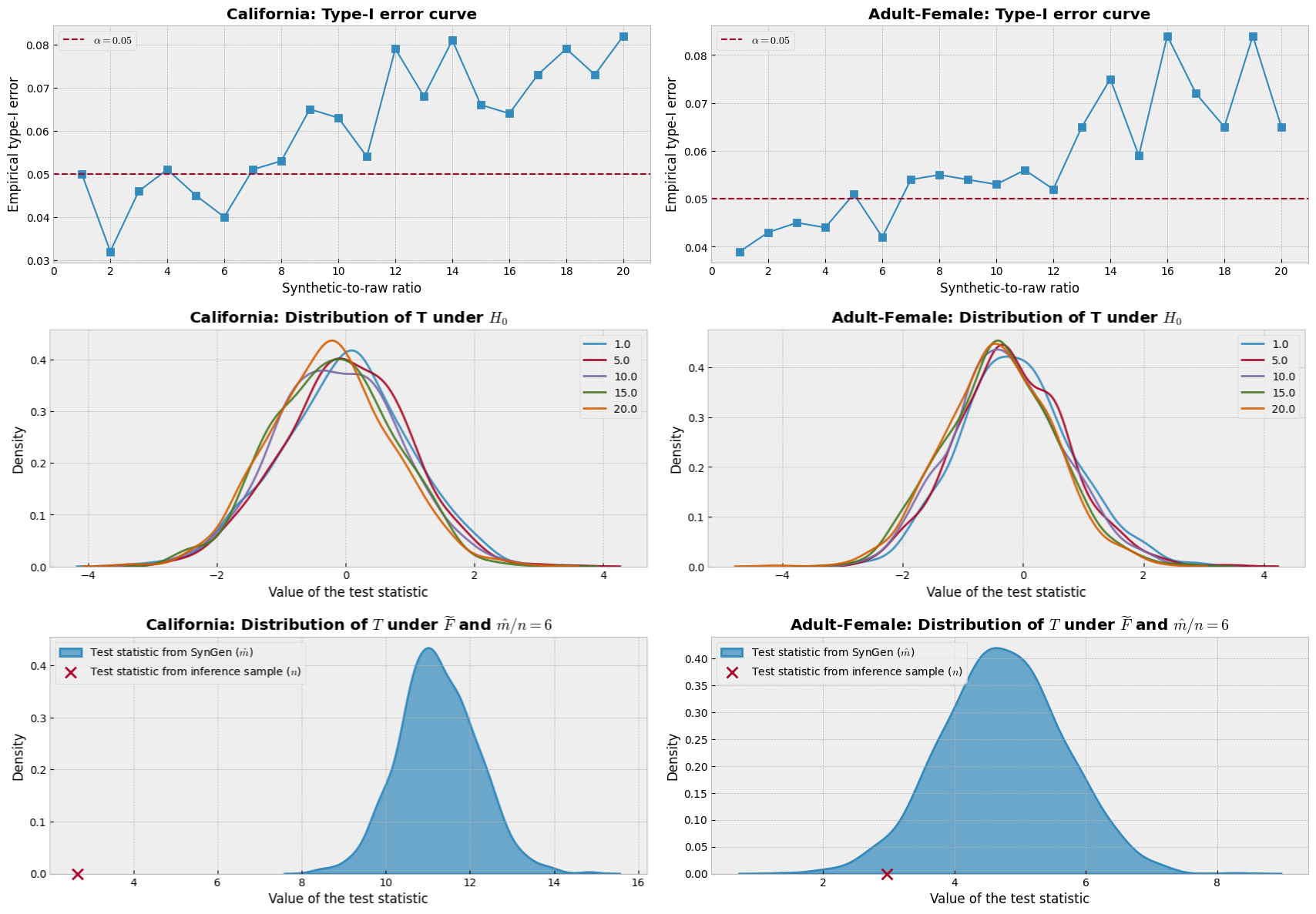
As depicted in Figure 5 (top left), the empirical Type-I error initially descends, then rises, ultimately surpassing the level as the ratio of synthetic-to-raw size grows. The estimated maximum ratio preserves the Type-I error control. In other words, we can augment the sample size to sixfold the raw sample size . This observation aligns with the generational effect we observed in predictive modeling for classification and regression. Consequently, notably enhances the power of Syn-Test, as indicated in Figure 5 (bottom left), where the test statistic distribution shifts to the right, increasing the power to reject when it is false.
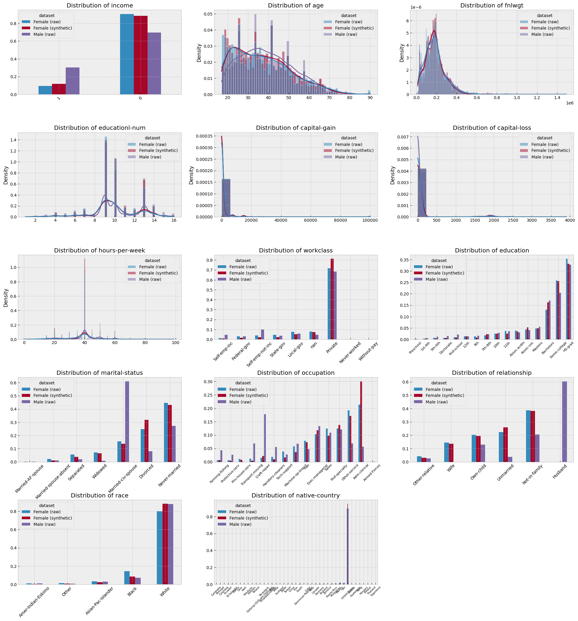
Knowledge Transfer Across Distinct Distributions. The Adult dataset concerns adult income for males and 16,192 females based on the census, including six numerical and eight nominal features, for example, age, work class, final weight, the number of years in education, marital status, working hours per week, and native country; see Kohavi et al. (1996) for more details. Our objective is to test if age, the number of years in education, and working hours per week are relevant to predicting if an adult female’s income surpasses the threshold of per year.
As Figure 6 depicts, the pronounced differences across genders exist in the distributions of categories like income, age, marital status, occupation, and relationship. A pertinent question arises: can adult male data augment the synthetic data generation and subsequent female analysis?
To harness this knowledge transfer, we pre-train a TDM solely on the adult-male data with observations. For hypothesis testing in (5), with a focus on adult females, we utilize a training sample of , divided evenly into and . Additionally, we use an inference sample consisting of . Following the Syn-Test approach as described in Figure 4, we use and for fine-tuning the pre-trained TDM and while using to avoid overfitting in model training and fine-tuning.
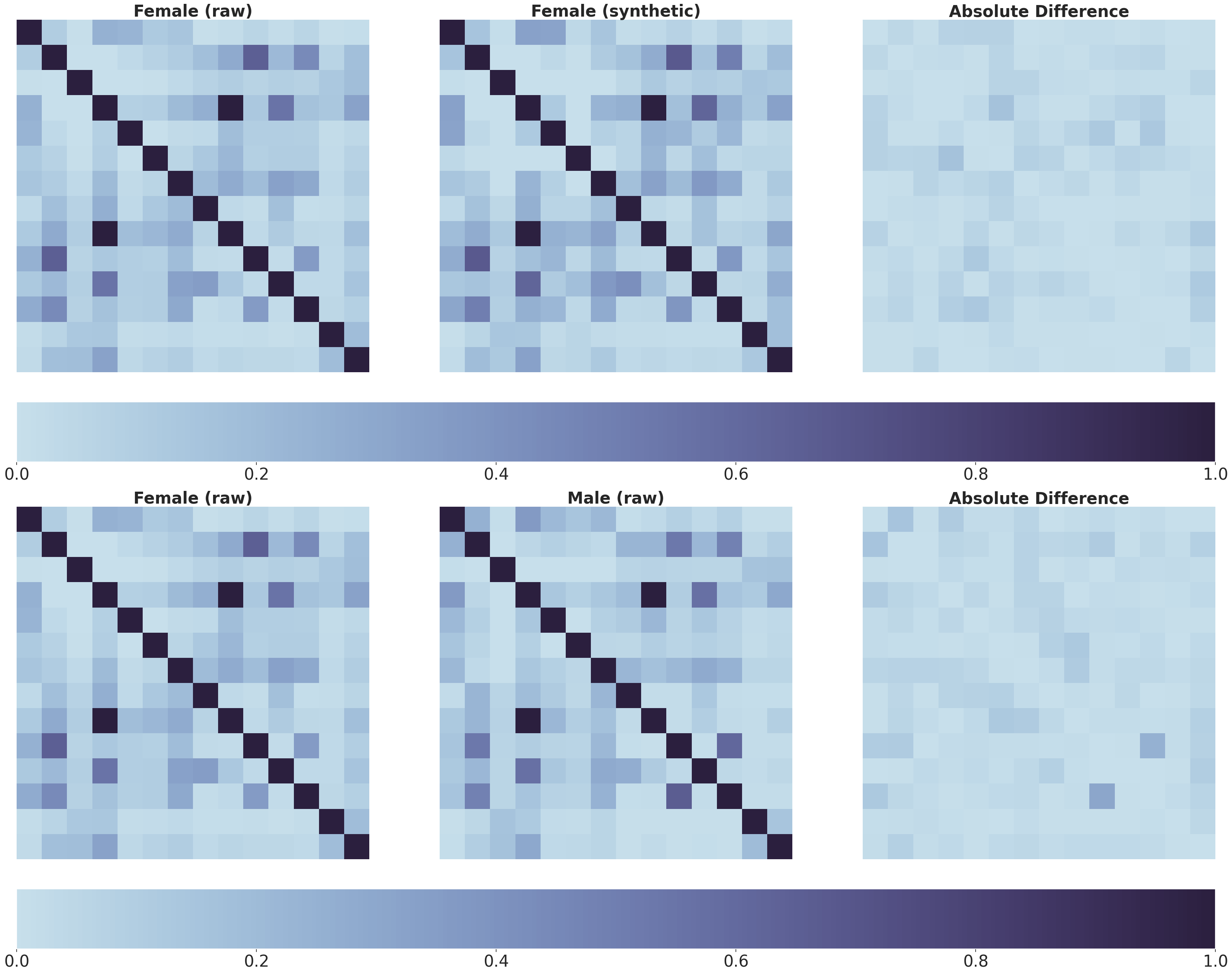
Figures 6 and 7 demonstrate that the synthetic female data produced by the diffusion model aligns more with the adult-female dataset than with the adult-male dataset. This alignment is evident by the Fréchet Inception Distance (FID), which measures the distributional differences between the generated and raw data vectors under the Gaussian assumption. The 1- and 2-Wasserstein distances between the empirical distributions of the two datasets provide further evidence (note that FID is 2-Wasserstein distance under Gaussian assumption). Notably, as shown in Table 3, the male-focused pre-trained TDM, once fine-tuned with a smaller female dataset, crafts synthetic female data with a diminished margin of error compared to models pre-trained on the adult-male data and adult-female data with individuals. This result confirms that leveraging pre-trained adult-male data with a somewhat distinct distribution can enhance the TDM’s generation precision for females. This empirical validation emphasizes the imperative of refining a pre-trained model to maximize knowledge transfer and achieve unparalleled accuracy.
Figure 5 highlights three key observations. First, the top two figures demonstrate that consistently controls the Type-I error of the Syn-Test across both scenarios. Second, the middle two figures suggest successful debiasing through synthetic data generation. Lastly, the bottom two plots exhibit a pronounced rightward shift in the test statistic distribution when comparing synthetic data to those derived from raw data. This shift signifies an enhancement in the test’s power, directly attributable to the augmentation of the sample size.
| FID (Gaussian) | 1-Wasserstein | 2-Wasserstein | |
|---|---|---|---|
| Female (raw) vs Male (raw) | 1.971 | 1.968 | 2.125 |
| Female (raw) vs Male (pre-trained) | 2.051 | 1.967 | 2.127 |
| Female (raw) vs Female (fine-tuned) | 0.249 | 1.170 | 1.399 |
4.3.2 Simulation
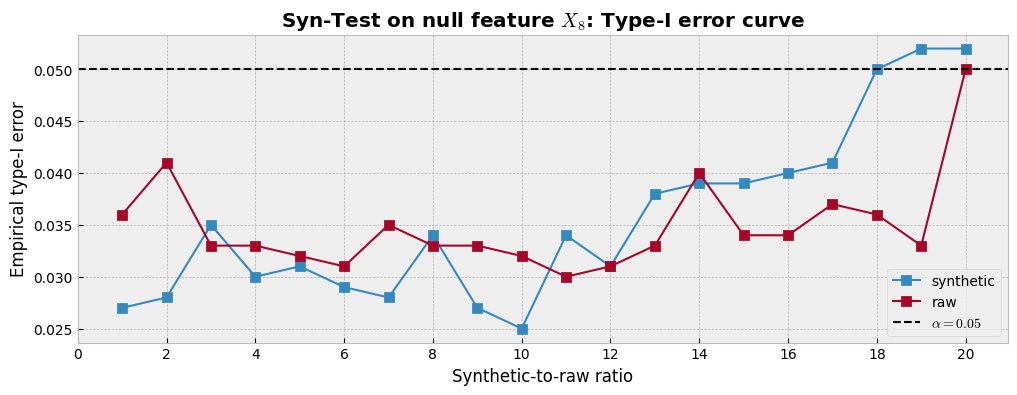
In this section, we evaluate the effectiveness of Syn-Test in controlling Type-I errors through simulation studies. We use the model in (4) with a modification: an additional feature, , is included but does not contribute to the model. Here, is distributed uniformly on (), and follows a normal distribution . We assess the relevance of the feature in prediction, thereby examining the control capability of Type-I error by Syn-Test. We will use the one-split test statistic proposed by (Dai, Shen and Pan, 2022) in Syn-Test, although we don’t rely on their asymptotic theory for the test statistic.
For our experiments, we split a raw sample into a training set and an inference set with and samples, respectively. Additionally, we use a distinct pre-training sample of to train the TDM on . This pre-trained model is subsequently fine-tuned on the raw training set according to the Syn-Test’s procedure. The inference sample, consisting of 200 instances, is utilized to validate the training of and for the test statistic in (6).
Moreover, we employ an MC size of with parameters and , and explore synthetic-to-raw ratios from to fine-tune the synthetic size .
As shown in Figure 8, the tuning curve of Syn-Test with synthetic data demonstrates a comparable performance to that of the same test when using independent raw data, particularly in terms of generational effect, while exhibiting similar patterns of variation. This finding indicates that Syn-Test effectively controls the Type-I error with synthetic data, aligning with observations from raw data. Finally, we adopt the conservative approach in selecting , choosing , in accordance with the guidelines in Section 2.3.
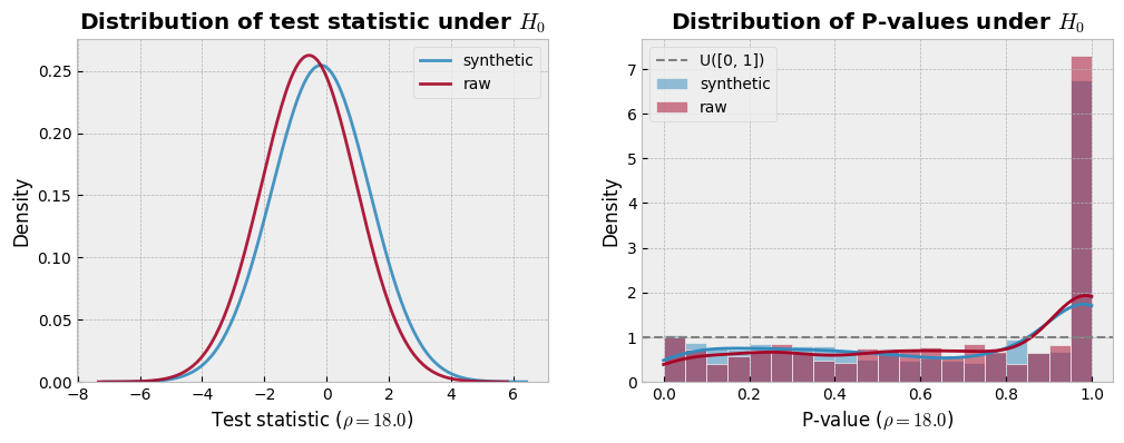
As illustrated in Figure 9, the estimated null distribution curve derived from synthetic data with closely resembles that based on independent raw data, albeit with a slight shift. This observation suggests minor generation errors by our generators. Furthermore, the distribution of P-values from Syn-Test using synthetic data under the null hypothesis with aligns well with that based on raw data. These plots demonstrate the effectiveness of Syn-Test in controlling Type-I error.
5 Data Privacy
The Syn framework can address privacy concerns using synthetic data generated by generative models trained to mimic the distribution of raw data. Unlike raw data, synthetic data imposes fewer privacy risks. However, it’s not entirely immune to reverse engineering attacks. These vulnerabilities mainly stem from the model’s parameters, which attackers could potentially infer from the synthetic data. In real-world applications like healthcare and finance, where data sensitivity is paramount, ensuring robust privacy measures is crucial.
To bolster data privacy, one may consider a privacy protection standard known as -differential privacy (Dwork et al., 2006), recognized as a gold standard in data privacy. Notably, it was implemented in the 2020 U.S. decennial census, demonstrating its practical applicability and effectiveness. This approach effectively safeguards against various privacy threats, including reverse engineering, re-identification, and inference attacks.
The definition of -differential privacy considers an adjacent realization differing from a realization of an original sample by just one observation. It revolves around a privatization mechanism , mapping from original dataset into a privatized version . For to be -differential private (Dwork et al., 2006), it satisfies: For any small and and any measurable set :
| (7) |
where is the privacy budget, controlling the strength of privacy protection. Smaller values indicate stronger privacy, while is a small probability allowance for the privacy guarantee, acknowledging minimal inherent risk. This definition accommodates -differential privacy with .
To generate synthetic data satisfying (7), we may employ techniques like Differentially Private Stochastic Gradient Descent (DP-SGD). DP-SGD injects a certain amount of Gaussian noise into the gradient updates during model training, ensuring that the model satisfies the desired privacy guarantees (Abadi et al., 2016). Differentially-private diffusion models (Ghalebikesabi et al., 2023) is an example of a point. This method is particularly effective in generating differentially private synthetic data while maintaining the utility of the data.
Unlike traditional differentially private samples, differentially private synthetic variants through these methods preserve the distributional characteristics of the original data. This preservation is advantageous as it can boost statistical analysis through sample size argumentation while enhancing privacy. However, this approach often requires more extensive model training due to the added noise, which can be a computational challenge.
6 Discussion: Future of Data Science
This article unveils the Syn paradigm—a novel approach to data analytics using high-fidelity synthetic data derived from real-world insights. By addressing challenges in traditional data analytics, such as data scarcity and privacy issues, this paradigm underscores that high-fidelity synthetic data can amplify the precision and efficiency of data analytics with sample size augmentation, as evidenced by the case studies herein. However, it is crucial to acknowledge the generational effect inherent to the Syn framework. Consequently, a fusion of reality and simulation is essential for unlocking the potential of synthetic data, offering fresh perspectives for both scientific and engineering domains.
The future of data science may pivot on our capability to harness raw and synthetic data. Large pre-trained generative models, equipped with extensive knowledge, offer a promising pathway. These frameworks distill domain knowledge, a testament being the successes of Generative Pre-trained Transformers in text and imagery contexts. As developing domain-centric generative models is gaining momentum, these generative models promise significant enhancements in synthetic data generation, paving the way for breakthroughs across a wide range of disciplines.
A systematic evaluation of the Syn framework across diverse applications is essential for advancing data science.
Appendix A Proofs
A.1 Proof of Theorem 2.1
Proof.
Let . The assumption that implies that . Moreover, note that if . Hence, when ,
Thus, by the definition of , that . This completes the proof. ∎
A.2 Proof of Theorem 2.2
A.3 Proof of Theorem 2.3
Proof.
Let be a random vector following and be one following . First, we bound the empirical distribution in (8), where for any . Let . Note that is a conditionally independent sample of size given following . By Hoeffding’s Lemma, a.s. for any , where is the conditional expectation with respect to given . By Markov’s inequality and the conditional independence between given , for any and ,
where denotes the probability, taking into account all sources of randomness.
For any , by choosing , we obtain that , with probability at least . On the other hand, given for any , where is a sample of size from . Using the union bound to combine these results, we obtain that
| (8) |
with probability at least . Note that .
Consequently, as in probability and , in probability. Using Syn-Test, the control of the empirical Type-I error at the level can be obtained as if we were using the true null distribution.
Concerning the power gain, note that . By definition and assumption, , indicating that .
This completes the proof. ∎
This work was supported in part by NSF grant DMS-1952539 and NIH grants R01AG069895, R01AG065636, R01AG074858, U01AG073079 (corresponding author: Xiaotong Shen, xshen@umn.edu).
Datasets \sdescription Information concerning datasets in Section 4: Case studies.
| Dataset | FB comments | Adult | House | California | Churn2 | Gesture | Aabalone | Insurance |
|---|---|---|---|---|---|---|---|---|
| Source | 2015 | 1996 | OpenML | 1997 | Kaggle | 2013 | OpenML | Kaggle |
| Sample size | 197080 | 48842 | 22784 | 20640 | 10000 | 9873 | 4177 | 1338 |
| Pre-training size | 157638 (80%) | 26048 (53%) | 14581 (64%) | 13209 (64%) | 6400 (64%) | 6318 (64%) | 2672 (64%) | 856 (64%) |
| Raw size | 19720 (10%) | 16281 (34%) | 4557 (20%) | 4128 (20%) | 2000 (20%) | 1975 (20%) | 836 (20%) | 268 (20%) |
| Test size | 19722 (10%) | 6513 (13%) | 3646 (16%) | 3303 (16%) | 1600 (16%) | 1580 (16%) | 669 (16%) | 214 (16%) |
| # Numerical features | 36 | 6 | 16 | 8 | 7 | 32 | 7 | 3 |
| # Nominal features | 15 | 8 | 0 | 0 | 4 | 0 | 1 | 3 |
References
- Abadi et al. (2016) {binproceedings}[author] \bauthor\bsnmAbadi, \bfnmMartin\binitsM., \bauthor\bsnmChu, \bfnmAndy\binitsA., \bauthor\bsnmGoodfellow, \bfnmIan\binitsI., \bauthor\bsnmMcMahan, \bfnmH Brendan\binitsH. B., \bauthor\bsnmMironov, \bfnmIlya\binitsI., \bauthor\bsnmTalwar, \bfnmKunal\binitsK. and \bauthor\bsnmZhang, \bfnmLi\binitsL. (\byear2016). \btitleDeep learning with differential privacy. In \bbooktitleProceedings of the 2016 ACM SIGSAC conference on computer and communications security \bpages308–318. \endbibitem
- Bi and Shen (2023) {barticle}[author] \bauthor\bsnmBi, \bfnmXuan\binitsX. and \bauthor\bsnmShen, \bfnmXiaotong\binitsX. (\byear2023). \btitleDistribution-invariant differential privacy. \bjournalJournal of Econometrics \bvolume235 \bpages444–453. \endbibitem
- Breiman (1997) {btechreport}[author] \bauthor\bsnmBreiman, \bfnmLeo\binitsL. (\byear1997). \btitleArcing the edge \btypeTechnical Report, \bpublisherCiteseer. \endbibitem
- Brown et al. (2020) {barticle}[author] \bauthor\bsnmBrown, \bfnmTom\binitsT., \bauthor\bsnmMann, \bfnmBenjamin\binitsB., \bauthor\bsnmRyder, \bfnmNick\binitsN., \bauthor\bsnmSubbiah, \bfnmMelanie\binitsM., \bauthor\bsnmKaplan, \bfnmJared D\binitsJ. D., \bauthor\bsnmDhariwal, \bfnmPrafulla\binitsP., \bauthor\bsnmNeelakantan, \bfnmArvind\binitsA., \bauthor\bsnmShyam, \bfnmPranav\binitsP., \bauthor\bsnmSastry, \bfnmGirish\binitsG., \bauthor\bsnmAskell, \bfnmAmanda\binitsA. \betalet al. (\byear2020). \btitleLanguage models are few-shot learners. \bjournalAdvances in neural information processing systems \bvolume33 \bpages1877–1901. \endbibitem
- Bubeck et al. (2023) {barticle}[author] \bauthor\bsnmBubeck, \bfnmSébastien\binitsS., \bauthor\bsnmChandrasekaran, \bfnmVarun\binitsV., \bauthor\bsnmEldan, \bfnmRonen\binitsR., \bauthor\bsnmGehrke, \bfnmJohannes\binitsJ., \bauthor\bsnmHorvitz, \bfnmEric\binitsE., \bauthor\bsnmKamar, \bfnmEce\binitsE., \bauthor\bsnmLee, \bfnmPeter\binitsP., \bauthor\bsnmLee, \bfnmYin Tat\binitsY. T., \bauthor\bsnmLi, \bfnmYuanzhi\binitsY., \bauthor\bsnmLundberg, \bfnmScott\binitsS. \betalet al. (\byear2023). \btitleSparks of artificial general intelligence: Early experiments with gpt-4. \bjournalarXiv preprint arXiv:2303.12712. \endbibitem
- Burden and Faires (2001) {bmisc}[author] \bauthor\bsnmBurden, \bfnmRL\binitsR. and \bauthor\bsnmFaires, \bfnmJD\binitsJ. (\byear2001). \btitleNumerical analysis 7th ed., brooks/cole, thomson learning. \endbibitem
- Carroll (2006) {barticle}[author] \bauthor\bsnmCarroll, \bfnmMichael W\binitsM. W. (\byear2006). \btitleThe movement for open access law. \bjournalLaw Library Journal \bvolume92 \bpages315. \endbibitem
- Chen et al. (2023) {barticle}[author] \bauthor\bsnmChen, \bfnmXuanting\binitsX., \bauthor\bsnmYe, \bfnmJunjie\binitsJ., \bauthor\bsnmZu, \bfnmCan\binitsC., \bauthor\bsnmXu, \bfnmNuo\binitsN., \bauthor\bsnmZheng, \bfnmRui\binitsR., \bauthor\bsnmPeng, \bfnmMinlong\binitsM., \bauthor\bsnmZhou, \bfnmJie\binitsJ., \bauthor\bsnmGui, \bfnmTao\binitsT., \bauthor\bsnmZhang, \bfnmQi\binitsQ. and \bauthor\bsnmHuang, \bfnmXuanjing\binitsX. (\byear2023). \btitleHow Robust is GPT-3.5 to Predecessors? A Comprehensive Study on Language Understanding Tasks. \bjournalarXiv preprint arXiv:2303.00293. \endbibitem
- Dai, Shen and Pan (2022) {barticle}[author] \bauthor\bsnmDai, \bfnmBen\binitsB., \bauthor\bsnmShen, \bfnmXiaotong\binitsX. and \bauthor\bsnmPan, \bfnmWei\binitsW. (\byear2022). \btitleSignificance tests of feature relevance for a black-box learner. \bjournalIEEE Transactions on Neural Networks and Learning Systems \bvolume//doi.org/10.1109/TNNLS.2022.3185742. \endbibitem
- Dinh, Krueger and Bengio (2014) {barticle}[author] \bauthor\bsnmDinh, \bfnmLaurent\binitsL., \bauthor\bsnmKrueger, \bfnmDavid\binitsD. and \bauthor\bsnmBengio, \bfnmYoshua\binitsY. (\byear2014). \btitleNice: Non-linear independent components estimation. \bjournalarXiv preprint arXiv:1410.8516. \endbibitem
- Dinh, Sohl-Dickstein and Bengio (2016) {barticle}[author] \bauthor\bsnmDinh, \bfnmLaurent\binitsL., \bauthor\bsnmSohl-Dickstein, \bfnmJascha\binitsJ. and \bauthor\bsnmBengio, \bfnmSamy\binitsS. (\byear2016). \btitleDensity estimation using real nvp. \bjournalarXiv preprint arXiv:1605.08803. \endbibitem
- Dorogush, Ershov and Gulin (2018) {barticle}[author] \bauthor\bsnmDorogush, \bfnmAnna V\binitsA. V., \bauthor\bsnmErshov, \bfnmVadim\binitsV. and \bauthor\bsnmGulin, \bfnmAndrey\binitsA. (\byear2018). \btitleCatBoost: unbiased boosting with categorical features. \bjournalarXiv preprint arXiv:1810.11363. \endbibitem
- Dwork et al. (2006) {binproceedings}[author] \bauthor\bsnmDwork, \bfnmCynthia\binitsC., \bauthor\bsnmKenthapadi, \bfnmKrishnaram\binitsK., \bauthor\bsnmMcSherry, \bfnmFrank\binitsF., \bauthor\bsnmMironov, \bfnmIlya\binitsI. and \bauthor\bsnmNaor, \bfnmMoni\binitsM. (\byear2006). \btitleOur data, ourselves: Privacy via distributed noise generation. In \bbooktitleAnnual International Conference on the Theory and Applications of Cryptographic Techniques \bpages486–503. \endbibitem
- Eastwood (2023) {barticle}[author] \bauthor\bsnmEastwood, \bfnmBrian\binitsB. (\byear2023). \btitleWhat is synthetic data — and how can it help you competitively? \bjournalMIT Sloan School. \endbibitem
- Efron (1992) {bincollection}[author] \bauthor\bsnmEfron, \bfnmBradley\binitsB. (\byear1992). \btitleBootstrap methods: another look at the jackknife. In \bbooktitleBreakthroughs in statistics \bpages569–593. \bpublisherSpringer. \endbibitem
- El Emam et al. (2021) {barticle}[author] \bauthor\bsnmEl Emam, \bfnmKhaled\binitsK., \bauthor\bsnmMosquera, \bfnmLucy\binitsL., \bauthor\bsnmJonker, \bfnmElizabeth\binitsE. and \bauthor\bsnmSood, \bfnmHarpreet\binitsH. (\byear2021). \btitleEvaluating the utility of synthetic COVID-19 case data. \bjournalJAMIA open \bvolume4 \bpagesooab012. \endbibitem
- Frid-Adar et al. (2018) {barticle}[author] \bauthor\bsnmFrid-Adar, \bfnmMaayan\binitsM., \bauthor\bsnmDiamant, \bfnmIdit\binitsI., \bauthor\bsnmKlang, \bfnmEyal\binitsE., \bauthor\bsnmAmitai, \bfnmMichal\binitsM., \bauthor\bsnmGoldberger, \bfnmJacob\binitsJ. and \bauthor\bsnmGreenspan, \bfnmHayit\binitsH. (\byear2018). \btitleGAN-based synthetic medical image augmentation for increased CNN performance in liver lesion classification. \bjournalNeurocomputing \bvolume321 \bpages321–331. \endbibitem
- Friedman (2002) {barticle}[author] \bauthor\bsnmFriedman, \bfnmJerome H\binitsJ. H. (\byear2002). \btitleStochastic gradient boosting. \bjournalComputational statistics & data analysis \bvolume38 \bpages367–378. \endbibitem
- Gao et al. (2023) {barticle}[author] \bauthor\bsnmGao, \bfnmCong\binitsC., \bauthor\bsnmKilleen, \bfnmBenjamin D\binitsB. D., \bauthor\bsnmHu, \bfnmYicheng\binitsY., \bauthor\bsnmGrupp, \bfnmRobert B\binitsR. B., \bauthor\bsnmTaylor, \bfnmRussell H\binitsR. H., \bauthor\bsnmArmand, \bfnmMehran\binitsM. and \bauthor\bsnmUnberath, \bfnmMathias\binitsM. (\byear2023). \btitleSynthetic data accelerates the development of generalizable learning-based algorithms for X-ray image analysis. \bjournalNature Machine Intelligence \bvolume5 \bpages294–308. \endbibitem
- Gartner (2022) {barticle}[author] \bauthor\bsnmGartner (\byear2022). \btitleIs Synthetic Data the Future of AI? \bjournalGartner Newsroom Q&A. \endbibitem
- Ghalebikesabi et al. (2023) {barticle}[author] \bauthor\bsnmGhalebikesabi, \bfnmSahra\binitsS., \bauthor\bsnmBerrada, \bfnmLeonard\binitsL., \bauthor\bsnmGowal, \bfnmSven\binitsS., \bauthor\bsnmKtena, \bfnmIra\binitsI., \bauthor\bsnmStanforth, \bfnmRobert\binitsR., \bauthor\bsnmHayes, \bfnmJamie\binitsJ., \bauthor\bsnmDe, \bfnmSoham\binitsS., \bauthor\bsnmSmith, \bfnmSamuel L\binitsS. L., \bauthor\bsnmWiles, \bfnmOlivia\binitsO. and \bauthor\bsnmBalle, \bfnmBorja\binitsB. (\byear2023). \btitleDifferentially private diffusion models generate useful synthetic images. \bjournalarXiv preprint arXiv:2302.13861. \endbibitem
- Hastie et al. (2009) {bbook}[author] \bauthor\bsnmHastie, \bfnmTrevor\binitsT., \bauthor\bsnmTibshirani, \bfnmRobert\binitsR., \bauthor\bsnmFriedman, \bfnmJerome H\binitsJ. H. and \bauthor\bsnmFriedman, \bfnmJerome H\binitsJ. H. (\byear2009). \btitleThe elements of statistical learning: data mining, inference, and prediction \bvolume2. \bpublisherSpringer. \endbibitem
- Ho, Jain and Abbeel (2020) {barticle}[author] \bauthor\bsnmHo, \bfnmJonathan\binitsJ., \bauthor\bsnmJain, \bfnmAjay\binitsA. and \bauthor\bsnmAbbeel, \bfnmPieter\binitsP. (\byear2020). \btitleDenoising diffusion probabilistic models. \bjournalAdvances in Neural Information Processing Systems \bvolume33 \bpages6840–6851. \endbibitem
- Hommel (1983) {barticle}[author] \bauthor\bsnmHommel, \bfnmGerhard\binitsG. (\byear1983). \btitleTests of the overall hypothesis for arbitrary dependence structures. \bjournalBiometrical Journal \bvolume25 \bpages423–430. \endbibitem
- Kiefer (1953) {barticle}[author] \bauthor\bsnmKiefer, \bfnmJack\binitsJ. (\byear1953). \btitleSequential minimax search for a maximum. \bjournalProceedings of the American mathematical society \bvolume4 \bpages502–506. \endbibitem
- Kim, Lee and Park (2022) {barticle}[author] \bauthor\bsnmKim, \bfnmJayoung\binitsJ., \bauthor\bsnmLee, \bfnmChaejeong\binitsC. and \bauthor\bsnmPark, \bfnmNoseong\binitsN. (\byear2022). \btitleStasy: Score-based tabular data synthesis. \bjournalarXiv preprint arXiv:2210.04018. \endbibitem
- Kingma and Dhariwal (2018) {barticle}[author] \bauthor\bsnmKingma, \bfnmDurk P\binitsD. P. and \bauthor\bsnmDhariwal, \bfnmPrafulla\binitsP. (\byear2018). \btitleGlow: Generative flow with invertible 1x1 convolutions. \bjournalAdvances in neural information processing systems \bvolume31. \endbibitem
- Kohavi et al. (1996) {binproceedings}[author] \bauthor\bsnmKohavi, \bfnmRon\binitsR. \betalet al. (\byear1996). \btitleScaling up the accuracy of naive-bayes classifiers: A decision-tree hybrid. In \bbooktitleKdd \bvolume96 \bpages202–207. \endbibitem
- Kotelnikov et al. (2023) {binproceedings}[author] \bauthor\bsnmKotelnikov, \bfnmAkim\binitsA., \bauthor\bsnmBaranchuk, \bfnmDmitry\binitsD., \bauthor\bsnmRubachev, \bfnmIvan\binitsI. and \bauthor\bsnmBabenko, \bfnmArtem\binitsA. (\byear2023). \btitleTabddpm: Modelling tabular data with diffusion models. In \bbooktitleInternational Conference on Machine Learning \bpages17564–17579. \bpublisherPMLR. \endbibitem
- Labrinidis and Jagadish (2012) {barticle}[author] \bauthor\bsnmLabrinidis, \bfnmAlexandros\binitsA. and \bauthor\bsnmJagadish, \bfnmHV\binitsH. (\byear2012). \btitleChallenges and opportunities with big data. \bjournalProceedings of the VLDB Endowment \bvolume5 \bpages2032–2033. \endbibitem
- Lee, Kim and Park (2023) {barticle}[author] \bauthor\bsnmLee, \bfnmChaejeong\binitsC., \bauthor\bsnmKim, \bfnmJayoung\binitsJ. and \bauthor\bsnmPark, \bfnmNoseong\binitsN. (\byear2023). \btitleCoDi: Co-evolving Contrastive Diffusion Models for Mixed-type Tabular Synthesis. \bjournalarXiv preprint arXiv:2304.12654. \endbibitem
- Lin et al. (2023) {barticle}[author] \bauthor\bsnmLin, \bfnmLequan\binitsL., \bauthor\bsnmLi, \bfnmZhengkun\binitsZ., \bauthor\bsnmLi, \bfnmRuikun\binitsR., \bauthor\bsnmLi, \bfnmXuliang\binitsX. and \bauthor\bsnmGao, \bfnmJunbin\binitsJ. (\byear2023). \btitleDiffusion models for time series applications: A survey. \bjournalarXiv preprint arXiv:2305.00624. \endbibitem
- Liu, Shen and Shen (2023) {barticle}[author] \bauthor\bsnmLiu, \bfnmYifei\binitsY., \bauthor\bsnmShen, \bfnmRex\binitsR. and \bauthor\bsnmShen, \bfnmXiaotong\binitsX. (\byear2023). \btitlePerturbation-Assisted Sample Synthesis: A Novel Approach for Uncertainty Quantification. \bjournalUnder revision for IEEE Transactions on Pattern Analysis and Machine Intelligencei. arXiv preprint arXiv:2305.18671. \endbibitem
- Liu and Xie (2020) {barticle}[author] \bauthor\bsnmLiu, \bfnmYaowu\binitsY. and \bauthor\bsnmXie, \bfnmJun\binitsJ. (\byear2020). \btitleCauchy combination test: a powerful test with analytic p-value calculation under arbitrary dependency structures. \bjournalJournal of the American Statistical Association \bvolume115 \bpages393–402. \endbibitem
- Liu et al. (2020) {barticle}[author] \bauthor\bsnmLiu, \bfnmQiao\binitsQ., \bauthor\bsnmXu, \bfnmJiaze\binitsJ., \bauthor\bsnmJiang, \bfnmRui\binitsR. and \bauthor\bsnmWong, \bfnmWing Hung\binitsW. H. (\byear2020). \btitleRoundtrip: A Deep Generative Neural Density Estimator. \bjournalarXiv preprint arXiv:2004.09017. \endbibitem
- Maas et al. (2011) {binproceedings}[author] \bauthor\bsnmMaas, \bfnmAndrew\binitsA., \bauthor\bsnmDaly, \bfnmRaymond E\binitsR. E., \bauthor\bsnmPham, \bfnmPeter T\binitsP. T., \bauthor\bsnmHuang, \bfnmDan\binitsD., \bauthor\bsnmNg, \bfnmAndrew Y\binitsA. Y. and \bauthor\bsnmPotts, \bfnmChristopher\binitsC. (\byear2011). \btitleLearning word vectors for sentiment analysis. In \bbooktitleProceedings of the 49th annual meeting of the association for computational linguistics: Human language technologies \bpages142–150. \endbibitem
- Madeo, Lima and Peres (2013) {binproceedings}[author] \bauthor\bsnmMadeo, \bfnmRenata CB\binitsR. C., \bauthor\bsnmLima, \bfnmClodoaldo AM\binitsC. A. and \bauthor\bsnmPeres, \bfnmSarajane M\binitsS. M. (\byear2013). \btitleGesture unit segmentation using support vector machines: segmenting gestures from rest positions. In \bbooktitleProceedings of the 28th Annual ACM Symposium on Applied Computing \bpages46–52. \endbibitem
- Oko, Akiyama and Suzuki (2023) {barticle}[author] \bauthor\bsnmOko, \bfnmKazusato\binitsK., \bauthor\bsnmAkiyama, \bfnmShunta\binitsS. and \bauthor\bsnmSuzuki, \bfnmTaiji\binitsT. (\byear2023). \btitleDiffusion Models are Minimax Optimal Distribution Estimators. \bjournalarXiv preprint arXiv:2303.01861. \endbibitem
- OpenAI (2023) {bmisc}[author] \bauthor\bsnmOpenAI (\byear2023). \btitleGPT-4 Technical Report. \endbibitem
- Pace and Barry (1997) {barticle}[author] \bauthor\bsnmPace, \bfnmR Kelley\binitsR. K. and \bauthor\bsnmBarry, \bfnmRonald\binitsR. (\byear1997). \btitleSparse spatial autoregressions. \bjournalStatistics & Probability Letters \bvolume33 \bpages291–297. \endbibitem
- Quionero-Candela et al. (2009) {bbook}[author] \beditor\bsnmQuionero-Candela, \bfnmJoaquin\binitsJ., \beditor\bsnmSugiyama, \bfnmMasashi\binitsM., \beditor\bsnmSchwaighofer, \bfnmAnton\binitsA. and \beditor\bsnmLawrence, \bfnmNeil D\binitsN. D., eds. (\byear2009). \btitleDataset shift in machine learning. \bpublisherThe MIT Press. \endbibitem
- Sanh et al. (2019) {barticle}[author] \bauthor\bsnmSanh, \bfnmVictor\binitsV., \bauthor\bsnmDebut, \bfnmLysandre\binitsL., \bauthor\bsnmChaumond, \bfnmJulien\binitsJ. and \bauthor\bsnmWolf, \bfnmThomas\binitsT. (\byear2019). \btitleDistilBERT, a distilled version of BERT: smaller, faster, cheaper and lighter. \bjournalarXiv preprint arXiv:1910.01108. \endbibitem
- Schapire (1990) {barticle}[author] \bauthor\bsnmSchapire, \bfnmRobert E\binitsR. E. (\byear1990). \btitleThe strength of weak learnability. \bjournalMachine learning \bvolume5 \bpages197–227. \endbibitem
- Shen, Bi and Shen (2022) {barticle}[author] \bauthor\bsnmShen, \bfnmXiaotong\binitsX., \bauthor\bsnmBi, \bfnmXuan\binitsX. and \bauthor\bsnmShen, \bfnmRex\binitsR. (\byear2022). \btitleData Flush. \bjournalHarvard data science review \bvolume4. \endbibitem
- Shwartz-Ziv and Armon (2022) {barticle}[author] \bauthor\bsnmShwartz-Ziv, \bfnmRavid\binitsR. and \bauthor\bsnmArmon, \bfnmAmitai\binitsA. (\byear2022). \btitleTabular data: Deep learning is not all you need. \bjournalInformation Fusion \bvolume81 \bpages84–90. \endbibitem
- Singh, Sandhu and Kumar (2015) {binproceedings}[author] \bauthor\bsnmSingh, \bfnmKamaljot\binitsK., \bauthor\bsnmSandhu, \bfnmRanjeet Kaur\binitsR. K. and \bauthor\bsnmKumar, \bfnmDinesh\binitsD. (\byear2015). \btitleComment volume prediction using neural networks and decision trees. In \bbooktitleIEEE UKSim-AMSS 17th International Conference on Computer Modelling and Simulation, UKSim2015 (UKSim2015). \endbibitem
- Sohl-Dickstein et al. (2015) {binproceedings}[author] \bauthor\bsnmSohl-Dickstein, \bfnmJascha\binitsJ., \bauthor\bsnmWeiss, \bfnmEric\binitsE., \bauthor\bsnmMaheswaranathan, \bfnmNiru\binitsN. and \bauthor\bsnmGanguli, \bfnmSurya\binitsS. (\byear2015). \btitleDeep unsupervised learning using nonequilibrium thermodynamics. In \bbooktitleInternational Conference on Machine Learning \bpages2256–2265. \bpublisherPMLR. \endbibitem
- Song, Meng and Ermon (2020) {barticle}[author] \bauthor\bsnmSong, \bfnmJiaming\binitsJ., \bauthor\bsnmMeng, \bfnmChenlin\binitsC. and \bauthor\bsnmErmon, \bfnmStefano\binitsS. (\byear2020). \btitleDenoising Diffusion Implicit Models. \bjournalarXiv:2010.02502. \endbibitem
- Sun et al. (2020) {binproceedings}[author] \bauthor\bsnmSun, \bfnmPei\binitsP., \bauthor\bsnmKretzschmar, \bfnmHenrik\binitsH., \bauthor\bsnmDotiwalla, \bfnmXerxes\binitsX., \bauthor\bsnmChouard, \bfnmAurelien\binitsA., \bauthor\bsnmPatnaik, \bfnmVijaysai\binitsV., \bauthor\bsnmTsui, \bfnmPaul\binitsP., \bauthor\bsnmGuo, \bfnmJames\binitsJ., \bauthor\bsnmZhou, \bfnmYin\binitsY., \bauthor\bsnmChai, \bfnmYuning\binitsY., \bauthor\bsnmCaine, \bfnmBenjamin\binitsB. \betalet al. (\byear2020). \btitleScalability in perception for autonomous driving: Waymo open dataset. In \bbooktitleProceedings of the IEEE/CVF conference on computer vision and pattern recognition \bpages2446–2454. \endbibitem
- Sweeney (2002) {barticle}[author] \bauthor\bsnmSweeney, \bfnmLatanya\binitsL. (\byear2002). \btitlek-anonymity: A model for protecting privacy. \bjournalInternational Journal of Uncertainty, Fuzziness and Knowledge-Based Systems \bvolume10 \bpages557–570. \endbibitem
- Topol (2019) {barticle}[author] \bauthor\bsnmTopol, \bfnmEric J\binitsE. J. (\byear2019). \btitleHigh-performance medicine: the convergence of human and artificial intelligence. \bjournalNature medicine \bvolume25 \bpages44–56. \endbibitem
- Tripuraneni, Jordan and Jin (2020) {barticle}[author] \bauthor\bsnmTripuraneni, \bfnmNilesh\binitsN., \bauthor\bsnmJordan, \bfnmMichael\binitsM. and \bauthor\bsnmJin, \bfnmChi\binitsC. (\byear2020). \btitleOn the theory of transfer learning: The importance of task diversity. \bjournalAdvances in neural information processing systems \bvolume33 \bpages7852–7862. \endbibitem
- Walonoski et al. (2018) {barticle}[author] \bauthor\bsnmWalonoski, \bfnmJason\binitsJ., \bauthor\bsnmKramer, \bfnmMark\binitsM., \bauthor\bsnmNichols, \bfnmJoseph\binitsJ., \bauthor\bsnmQuina, \bfnmAndre\binitsA., \bauthor\bsnmMoesel, \bfnmChris\binitsC., \bauthor\bsnmHall, \bfnmDylan\binitsD., \bauthor\bsnmDuffett, \bfnmCarlton\binitsC., \bauthor\bsnmDube, \bfnmKudakwashe\binitsK., \bauthor\bsnmGallagher, \bfnmThomas\binitsT. and \bauthor\bsnmMcLachlan, \bfnmScott\binitsS. (\byear2018). \btitleSynthea: An approach, method, and software mechanism for generating synthetic patients and the synthetic electronic health care record. \bjournalJournal of the American Medical Informatics Association \bvolume25 \bpages230–238. \endbibitem
- Wasserman, Ramdas and Balakrishnan (2020) {barticle}[author] \bauthor\bsnmWasserman, \bfnmLarry\binitsL., \bauthor\bsnmRamdas, \bfnmAaditya\binitsA. and \bauthor\bsnmBalakrishnan, \bfnmSivaraman\binitsS. (\byear2020). \btitleUniversal inference. \bjournalProceedings of the National Academy of Sciences \bvolume117 \bpages16880–16890. \endbibitem
- Wasserman and Roeder (2009) {barticle}[author] \bauthor\bsnmWasserman, \bfnmLarry\binitsL. and \bauthor\bsnmRoeder, \bfnmKathryn\binitsK. (\byear2009). \btitleHigh dimensional variable selection. \bjournalAnnals of statistics \bvolume37 \bpages2178. \endbibitem
- Wei et al. (2021) {barticle}[author] \bauthor\bsnmWei, \bfnmDonglai\binitsD., \bauthor \betalet al. (\byear2021). \btitleDiffusion Models Beat GANs on Image Synthesis. \bjournalPreprint arXiv. \endbibitem
- Xie et al. (2018) {barticle}[author] \bauthor\bsnmXie, \bfnmLiyang\binitsL., \bauthor\bsnmLin, \bfnmKaixiang\binitsK., \bauthor\bsnmWang, \bfnmShu\binitsS., \bauthor\bsnmWang, \bfnmFei\binitsF. and \bauthor\bsnmZhou, \bfnmJiayu\binitsJ. (\byear2018). \btitleDifferentially private generative adversarial network. \bjournalarXiv preprint arXiv:1802.06739. \endbibitem
- Yuan et al. (2023) {barticle}[author] \bauthor\bsnmYuan, \bfnmYuan\binitsY., \bauthor\bsnmDing, \bfnmJingtao\binitsJ., \bauthor\bsnmShao, \bfnmChenyang\binitsC., \bauthor\bsnmJin, \bfnmDepeng\binitsD. and \bauthor\bsnmLi, \bfnmYong\binitsY. (\byear2023). \btitleSpatio-temporal Diffusion Point Processes. \bjournalarXiv preprint arXiv:2305.12403. \endbibitem
- Zhang et al. (2023) {barticle}[author] \bauthor\bsnmZhang, \bfnmChenshuang\binitsC., \bauthor\bsnmZhang, \bfnmChaoning\binitsC., \bauthor\bsnmZhang, \bfnmMengchun\binitsM. and \bauthor\bsnmKweon, \bfnmIn So\binitsI. S. (\byear2023). \btitleText-to-image diffusion model in generative ai: A survey. \bjournalarXiv preprint arXiv:2303.07909. \endbibitem
- Zheng and Charoenphakdee (2022) {barticle}[author] \bauthor\bsnmZheng, \bfnmShuhan\binitsS. and \bauthor\bsnmCharoenphakdee, \bfnmNontawat\binitsN. (\byear2022). \btitleDiffusion models for missing value imputation in tabular data. \bjournalarXiv preprint arXiv:2210.17128. \endbibitem