Transporting treatment effects from difference-in-differences studies

Abstract

Difference-in-differences (DID) is a popular approach to identify the causal effects of treatments and policies in the presence of unmeasured confounding. DID identifies the sample average treatment effect in the treated (SATT). However, a goal of such research is often to inform decision-making in target populations outside the treated sample. Transportability methods have been developed to extend inferences from study samples to external target populations; these methods have primarily been developed and applied in settings where identification is based on conditional independence between the treatment and potential outcomes, such as in a randomized trial. This paper develops identification and estimators for effects in a target population, based on DID conducted in a study sample that differs from the target population. We present a range of assumptions under which one may identify causal effects in the target population and employ causal diagrams to illustrate these assumptions. In most realistic settings, results depend critically on the assumption that any unmeasured confounders are not effect measure modifiers on the scale of the effect of interest. We develop several estimators of transported effects, including a doubly robust estimator based on the efficient influence function. Simulation results support theoretical properties of the proposed estimators. We discuss the potential application of our approach to a study of the effects of a US federal smoke-free housing policy, where the original study was conducted in New York City alone and the goal is extend inferences to other US cities.

Keywords: difference-in-differences, transportability, efficiency, causal inference

1 Introduction

Difference-in-differences (DID) is a popular identification strategy when studying the causal effects of large-scale social and economic policies [1, 2]. DID is appealing when: (i) randomization is not feasible, (ii) there is variation across jurisdictions and over time in terms of whether a policy was adopted, and (iii) not all variables that are confounders of the policy-outcome relationship are measured, leading to concerns about confounding bias [3]. By comparing pre- and post-policy outcomes in both the jurisdiction implementing the policy and a comparable jurisdiction without the policy, and making a so-called parallel trends assumption (i.e., that changes in average potential outcomes over time are independent of policy adoption) [1, 4], DID can identify the causal effect of the policy on the outcome, even in settings where unmeasured variables would confound either (i) a pre-post analysis or (ii) a post-policy comparison between the treated and untreated jurisdictions.

An important (often under-recognized) aspect of DID is that it identifies the average treatment effect among the treated (ATT) in the post-policy period, and not the average treatment effect (ATE) or other common parameters of interest [1]. For example, the ATT in a study of a policy raising the minimum wage is the effect of the policy on outcomes for the population living in the jurisdiction(s) that actually raised the minimum wage, and not the population living in all the jurisdictions in the study—those with and without the policy. ATT estimates resulting from a DID analysis can be informative as to whether to maintain or discontinue policies in those locations. However, a major goal of DID research is often to inform policy decisions by governments that have not yet adopted the policy of interest; in the minimum wage example, it may be of interest to inform decisions by the federal government or states with less generous minimum wage laws. Naïvely considering the estimated policy effects to apply to untreated jurisdictions requires the additional, strong assumption that there are no effect measure modifiers (measured or unmeasured) whose distribution varies between the treated jurisdiction(s) under study and the untreated jurisdiction(s) to which one wishes to make inferences [5, 6]. For example, such an extrapolation would be biased if effects of the minimum wage differ by age, and age distributions differed across states.

Generalizability and transportability methods have been developed with the goal of formally extending inferences made in one population to another population in the presence of effect heterogeneity [7, 8, 9]. These methods have mainly been applied in contexts where internal validity is established based on an unconfoundedness assumption, typically achieved through a randomized controlled trial (RCT). It is well-known that real-world RCTs can deliver high internal validity, but that inferences from such studies apply only to the people participating in the RCT, which may differ from the true target population in terms of effects experienced. We define “target population” to be the population to whom inference is desired, as dictated by substantive concerns. For example, in RCTs of medical treatments, the target population may be the population that should receive treatments in practice, which may differ in important aspects from the individuals included in the trial [10, 11]. Methods exist to quantitatively extend (i.e., transport or generalize) effects estimated in RCTs to target populations other than the included study sample, possibly alleviating the well-known tradeoff between internal and external validity in such studies [12].

It is plausible that transportablity methods could be used to quantitatively extend causal effects estimated from DID studies to target populations other than the treated sample, possibly alleviating the well-known tradeoff between internal and external validity in such DID studies as well. However, to our knowledge, neither identification assumptions nor estimators for transporting DID estimates have been addressed in the literature. DID presents special challenges for transportability because of the presumed existence of unmeasured confounders. Standard approaches to transportability assume that a conditional average treatment effect is constant between the sample and target population after conditioning on a measured set of covariates; if any unmeasured confounders in a DID application are also effect measure modifiers of the treatment-outcome relationship, then the existence of these unmeasured confounders creates complexities in evaluating this condition which have not, to our knowledge, been explored. Causal diagrams [13] may facilitate such an exploration, as they have been essential in understanding assumptions for identification of transported effects [14, 6, 9], but have seen limited use in DID settings [4, 15]. This disconnect may be because causal diagrams generally only capture nonparametric independence assumptions [13], whereas parallel trends is a semiparametric assumption partially restricting the functional form of the outcome distribution [16].

This paper develops a formal approach to identification and estimation of effects in a target population, based on DID conducted in a study sample that differs from the target population. This paper is framed as transportability in the sense that we assume the study sample is not a subset of the target population [17, 8], though our results can easily be extended to the case where the study sample is nested within the target population. We employ causal diagrams to understand the sampling mechanism (i.e, the model that distinguishes the study sample from the target population), and show that our results rely crucially on the assumption that unmeasured confounders are either independent of the sampling process or are not effect modifiers on the scale of the effect being estimated (in this paper, we focus on additive effects such as the ATT and ATE, but our results can be generalized to non-additive measures, such as risk ratios). Section 2 describes the observed data and preliminary assumptions, Section 3 presents key identification results linking the observed data in the sample to causal quantities in the target population, and Section 4 presents estimators (including a doubly robust estimator based on the efficient influence function) for these quantities, which are illustrated using simulation in Section 5. Section 6 concludes.

2 Preliminaries

Suppose we observe data on the variables $W_{i},A_{i},Y_{i0}$, and $Y_{i1}$ in a study sample containing $n$ individuals or units ($i=1,...,n$), where $W_{i}$ are (possibly multivariate) baseline covariates measured just before exposure, $A_{i}$ is a binary exposure, and $Y_{it}$ $(t=0,1)$ are outcomes measured before ($t=0$) and after ($t=1$) exposure occurs. Hereafter, we drop the $i$ subscript unless needed to resolve ambiguity. Suppose that the study sample is not representative of the true target population of interest, and that the latter contains $N$ individuals ($i=1,...,N$). We let $S=1$ denote membership in the study sample and $S=0$ denote membership in the target population. We assume that outcomes are only measured in the study sample, but that treatment and covariates are measured in both the study sample and the target population. Thus, the observed data take the form $O=\{S,A,W,Y_{0}S,Y_{1}S\}.$ Throughout, we use $f(x|\cdot)$ to denote a conditional density if $x$ is continuous and a conditional probability mass function if $x$ is discrete. Caligraphic uppercase letters denote the support of a random variable.

We use $Y_{t}(a)$ to denote a potential outcome, or the outcome that would have occurred if exposure $A$ had been set by intervention to the value $a$. We assume the following throughout:

Assumption 1.

(No interference) $Y_{it}(a_{i},a_{i^{\prime}})=Y_{it}(a_{i})$ for $i\neq i^{\prime}$, with $i,i^{\prime}$ such that $\{S_{i},S_{i^{\prime}}\}\in\{0,1\}^{2}$

Assumption 2.

(Treatment version irrelevance) If $A_{i}=a$, then $Y_{it}=Y_{it}(a)$ with $i,i^{\prime}$ such that $\{S_{i},S_{i^{\prime}}\}\in\{0,1\}^{2}$

Assumptions 1 and 2 are standard in the causal inference and transportability literature and are not specific to the DID setting. Assumption 1 requires that one unit’s treatment does not impact another unit’s potential outcome in either the sample or the target. Assumption 2 requires that treatments are sufficiently well-defined that observed outcomes can stand in for potential outcomes under treatment with the observed exposures, and that versions of the treatment do not differ between the sample and target. Assumptions 1 and 2 are often referred to together as the stable unit treatment value assumption (SUTVA).

2.1 Difference-in-differences in the study sample

Here, we give a brief review of causal identification based on DID, which we will assume is the basis of identification in the study sample. Specifically, we invoke the following assumptions, standard in the DID literature [18, 19, 1]:

Assumption 3.

(No anticipation): $Y_{0}(a)=Y_{0}$ for $a=0,1$

Assumption 4.

(Positivity of treatment assignment) If $f(w|S=1)>0$ then $f(A=0|W=w,S=1)>0$ with probability 1 for all $w\in\mathcal{W}$

Assumption 5.

(Parallel Trends): For $w\in\mathcal{W}$:

$$\mathbb{E}\{Y_{t}(0)-Y_{t-1}(0)|A=1,S=1,W=w\}=\mathbb{E}\{Y_{t}(0)-Y_{t-1}(0)|A=0,S=1,W=w\}$$

Assumption 3 states that future treatment does not impact the prior outcomes (this assumption can also be relaxed to allow anticipation up to a known time period [20]). It is well known that under Assumptions 1-5, it is possible to identify the $W$-conditional SATT, defined as $\eta(w)\equiv\mathbb{E}[Y_{1}(1)-Y_{1}(0)|W=w,A=1,S=1].$ Specifically, under Assumptions 1-5 we have:

$$\eta(w) =\mathbb{E}[Y_{1}-Y_{0}|W=w,A=1,S=1]-\mathbb{E}[Y_{1}-Y_{0}|W=w,A=0,S=1]$$ (1)

$$\equiv m_{1}(w)-m_{0}(w),$$

where we define $m_{a}(w)=\mathbb{E}[Y_{1}-Y_{0}|W=w,A=a,S=1]$. By extension, the unconditional sample ATT (abbreviated SATT, usually the focal parameter in DID) is identified as $\mathbb{E}[Y_{1}(1)-Y_{1}(0)|A=1,S=1]=\mathbb{E}[m_{1}(W)-m_{0}(W)|A=1,S=1].$ However, and importantly for our discussion, Assumptions 1-5 are not sufficient to identify parameters unconditional on $A=1$, such as the sample average treatment effect (SATE), defined as $\mathbb{E}[Y_{1}(1)-Y_{1}(0)|S=1].$ This is because parallel trends provides information about potential outcomes only among the treated group; without further assumptions there is no basis for identification of potential outcomes for the group $A=0$. Moreover, and as is the focus of this paper, additional assumptions would be required to identify effects outside the study sample, since parallel trends and positivity of treatment assignment are conditional on $S=1$.

3 Identification of transported treatment effects

In this section we consider the task of equating a causal estimand (i.e., one specified in terms of potential outcomes) in the target population to a function of the distribution of the observed data, $O$. Specifically, we focus on the population average treatment effect in the treated (PATT), defined as $\mathbb{E}[Y_{1}(1)-Y_{1}(0)|A=1,S=0]$, and the population average treatment effect (PATE) defined as $\mathbb{E}[Y_{1}(1)-Y_{1}(0)|S=0]$. We begin by introducing a motivating example, after which we introduce and discuss a set of sufficient identifying assumptions, and present identifying formulas which equal each causal estimand if the assumptions are true.

3.1 Motivating example

As of July 30, 2018, a US Department of Housing and Urban Development (HUD) rule required all public housing authorities to implement smoke-free housing (SFH) policies banning smoking in residences. As a motivating example, consider the question, what effect did the federal SFH policy have on air quality in US public housing developments? To answer this question, we consider transporting the results from a study conducted in public housing buildings in New York City (NYC) only. Specifically, a team of investigators conducted air quality monitoring in living rooms and common areas of NYC public housing buildings, both before the federal policy went into effect (from April to July 2018), and again approximately every six months for 3 years post-policy. A DID analysis was conducted to estimate the effect of the policy on indoor air nicotine (among other measures), using as a comparison group a sample of households receiving housing assistance through a program known as Section 8, a public subsidy to supplement rental costs in private sector buildings [21]. Air quality was sampled in stairwells, hallways, and living rooms; for simplicity here we focus on stairwells. Because of concerns about systematic variation in outdoor air quality between building types, the investigators adjusted for outdoor ambient PM_2.5 in their DID estimates. (We note that in the original study, building inclusion criteria were high-rise [$>$15 floors], large resident population [$>$150 units], at least 80% Black or Hispanic residents, and at least 20% younger than 18 years; for simplicity we ignore these criteria here.)

In this example, $Y_{t}$ is a continuous variable representing log-transformed air nicotine in stairwells (where we let $t=0$ denote April-July 2018 and $t=1$ denote April-September 2021), $A=1$ denotes residence in a public housing building, $A=0$ denotes residence in a Section 8 household, $S=1$ denotes residence in NYC, $S=0$ denotes residence outside of NYC, and $W$ is a continuous variable capturing outdoor ambient PM_2.5. Thus, if Assumptions 1-5 hold (along with correct model specification and no measurement error), the DID results in this study may be interpreted as estimates of the effect of the SFH policy on indoor air quality for NYC public housing residents only. Though the study is informative as to the effect of the policy in NYC, it is also of interest to federal policymakers to estimate the PATT, which here represents the effect of the HUD rule on air nicotine in April-September 2021 in public housing in the US outside of NYC ($S=0$). Moreover, it may also be of interest to assess the PATE, which here represents the effect of a hypothetical policy covering both public housing and Section 8 housing. Importantly, the estimates in this study cannot be interpreted as estimates of the PATT or PATE without additional assumptions.

3.2 Naïve approach

We begin with an approach to transportability that does not take into account the causal structure of DID (in particular, does not take into account unmeasured confounding), after which we will use causal diagrams to illustrate why this approach will usually fail. Since all identified potential outcomes in equation (1) are conditional on $A=1$, an obvious starting point in attempting to transport effects identified through DID is to identify the PATT. Inspecting equation (1), a natural approach may be to assume that the $W$-conditional SATTs (conditional on each value of $w$) are equal between the sample and the target. If this were the case, one could identify the PATT using the following expression:

$$\mathbb{E}[Y_{1}^{1}-Y_{1}^{0}|A=1,S=0] =\mathbb{E}[\mathbb{E}(Y_{1}^{1}-Y_{1}^{0}|W,A=1,S=1)|A=1,S=0]$$

$$=\mathbb{E}[m_{1}(W)-m_{0}(W)|A=1,S=0]$$ (2)

Specifically, in order for equation (2) to hold, the following assumptions would be sufficient:

Assumption 6.

(Exchangeability of selection) $Y_{t}(a)\mathchoice{\mathrel{\hbox to0.0pt{$\displaystyle\perp$\hss}\mkern 2.0mu{\displaystyle\perp}}}{\mathrel{\hbox to0.0pt{$\textstyle\perp$\hss}\mkern 2.0mu{\textstyle\perp}}}{\mathrel{\hbox to0.0pt{$\scriptstyle\perp$\hss}\mkern 2.0mu{\scriptstyle\perp}}}{\mathrel{\hbox to0.0pt{$\scriptscriptstyle\perp$\hss}\mkern 2.0mu{\scriptscriptstyle\perp}}}S|W,A=1$

Assumption 7.

(Positivity of selection) If $f(w|A=1,S=0)>0$ then $f(S=1|W=w,A=1)>0$ with probability 1 for all $w\in\mathcal{W}$

Assumption 6 states that, among the treated group, the distributions of potential outcomes in the sample and target are equal after conditioning on $W$. Assumption 7 states that any covariate values that may occur in the target treated group must also be possible in the sample treated group. Assumptions 6 and 7 together imply that the $W$-conditional ATT is constant across settings, and hence that the PATT is identified by equation (2).

Though Assumption 6 is similar to the exchangeability of selection assumption usually invoked for transportability of the average treatment effect (ATE), it differs importantly in that it must hold conditional on $A=1.$ This is so because DID was the basis for identification in the sample, so any effects identified in the sample (whether SATT or $W$-conditional SATT) are conditional on $A=1$, and the basis for transportability is therefore the constancy of the $W$-conditional SATTs (not SATEs) across settings. This constancy is dependent on replacing potential outcomes in the treated target with those in the treated sample, and for this replacement to be licensed, Assumption 6 must condition on $A=1$.

Unfortunately, conditioning on $A=1$ means Assumption 6 is unlikely to hold in most DID applications. To illustrate this point, Figure 1(a) displays a single world intervention graph (SWIG) depicting a common DID setting. SWIGs are similar to causal directed acyclic graphs (DAGs) in that nodes represent random variables, directed arrows represent direct effects, and conditional independencies are given by d-separation rules [22]. SWIGs extend DAGs by depicting interventions on variables as split nodes ($A|a$ in Figure 1(a) indicates intervening to set $A=a$), and any variables affected by the intervention variable become potential outcomes under that intervention. Figure 1(a) represents a standard DID scenario in the sense that $U$ represents unmeasured common causes of $A$ and $Y_{1}$ that would confound a cross-sectional comparison, and whose existence motivates the use of DID. In Figure 1(b), we add $S$ with arrows into $A$ and $W$, depicting the assumption that distributions of these variables differ across settings. Following the convention of selection diagrams, arrows emanating from $S$ represent “exogenous conditions that determine the values of the variables to which they point” [14]. Assumption 6 would not be expected to hold in Figure 1(b) due to the existence of the path $S\rightarrow A\leftarrow U\rightarrow Y_{1}(a)$, on which $A$ is a collider. Thus, this path is opened by conditioning on $A$ (and not closed by conditioning on $W$), rendering $S$ potentially associated with $Y_{1}(a)$ conditional on $\{W,A=1\}$. For the same reason, $S$ would also be associated with $Y_{0}$ conditional on $\{W,A=1\}$ in at least one data distribution consistent with the SWIG. Importantly, such paths will be present whenever (i) there is unmeasured confounding, and (ii) the target and sample differ in the distribution of treatment (conditional on $W$). We expect (i) to always be the case (otherwise DID would be unnecessary). We also expect (ii) to be the case except in rare circumstances such as when $A$ is experimentally assigned in both the target and the sample. Importantly, this failure of Assumption 6 occurs regardless of whether the unmeasured confounders $U$ differ marginally in distribution between the target and sample (i.e., whether or not there is an arrow from $S$ into $U$ in Figure 1(b)).

(a)

(b)

Figure 1: Single world intervention graphs (SWIGs) illustrating common scenarios relevant for (a) DID in a sample and (b) transportability of DID results to a target population. Double-headed arrows indicate unmeasured common causes between two nodes.

3.3 Identification via restrictions on effect heterogeneity

The analysis in the previous subsection illustrated that identification of transported effects based on exchangeability according to measured covariates (as in Assumption 6) is unlikely to be tenable in DID studies, since conditioning on $A=1$ will typically cause unmeasured covariates $U$ to be associated with the sampling mechanism $S$ regardless of whether this association exists marginally. Thus, Assumption 6 would likely only be plausible if $U$ were included in the conditioning event, but this would not aid identification since $U$ is unmeasured. Fortunately, it is possible to identify transported effects when variables needed for exchangeability are unmeasured, so long as those variables are not also effect measure modifiers on the scale on which the causal effects are being measured, which we illustrate here.

We begin by expressing the concept that unmeasured confounders $U$ drive our decision to use DID by stating the following Assumptions, which relate only to identification in the sample:

Assumption 8.

(Latent exchangeability of treatment) $Y_{t}(a)\mathchoice{\mathrel{\hbox to0.0pt{$\displaystyle\perp$\hss}\mkern 2.0mu{\displaystyle\perp}}}{\mathrel{\hbox to0.0pt{$\textstyle\perp$\hss}\mkern 2.0mu{\textstyle\perp}}}{\mathrel{\hbox to0.0pt{$\scriptstyle\perp$\hss}\mkern 2.0mu{\scriptstyle\perp}}}{\mathrel{\hbox to0.0pt{$\scriptscriptstyle\perp$\hss}\mkern 2.0mu{\scriptscriptstyle\perp}}}A|W,U,S=1$ for $t\in\{0,1\}$ and $a\in\{0,1\}$

Assumption 9.

(Latent positivity of treatment) If $f(u,w|S=1)>0$ then $f(A=a|U=u,W=w,S=1)>0$ with probability 1 for $a\in\{0,1\}$ and $\{u,w\}\in\{\mathcal{U},\mathcal{W}\}$

In a sense, Assumption 8 does not introduce any new restrictions because one can define $U$ to be whatever variables (known or unknown) confound the cross-sectional association between $A$ and $Y_{t}$ and which motivate the use of DID in the first place. In contrast, Assumption 9 may be restrictive; the requirement that unmeasured confounding variables $U$ (known or unknown) have overlapping distribution between the treated and untreated may not hold in some settings and is not necessary for identification of the SATT via DID. (As an aside, it can be shown that parallel trends will hold if (i) Assumptions 9 and 8 hold and (ii) $U$ exerts a constant effect on $Y_{0}$ and $Y_{1}$ on the additive scale within levels of $W$ among the treated [4]. However, in this paper we assume parallel trends to hold and do not consider what conditions render it plausible or not.) Next consider the follow assumptions aimed at identification in the target:

Assumption 10.

(Latent exchangeability of selection) $Y_{t}(a)\mathchoice{\mathrel{\hbox to0.0pt{$\displaystyle\perp$\hss}\mkern 2.0mu{\displaystyle\perp}}}{\mathrel{\hbox to0.0pt{$\textstyle\perp$\hss}\mkern 2.0mu{\textstyle\perp}}}{\mathrel{\hbox to0.0pt{$\scriptstyle\perp$\hss}\mkern 2.0mu{\scriptstyle\perp}}}{\mathrel{\hbox to0.0pt{$\scriptscriptstyle\perp$\hss}\mkern 2.0mu{\scriptscriptstyle\perp}}}S|W,U,A$ for $t\in\{0,1\}$ and $a\in\{0,1\}$

Assumption 11.

(Latent positivity of selection) If $f(u,w|A=a,S=0)>0$ then $f(S=1|U=u,W=w,A=a)>0$ with probability 1 for $a\in\{0,1\}$ and $\{u,w\}\in\{\mathcal{U},\mathcal{W}\}$

Assumption 10 modifies Assumption 6 by allowing for $U$ in the conditioning event, so that the potential outcomes are equal in distribution between the sample and the target after conditioning on $W$, $U$, and $A$. Similarly, Assumption 11 requires all possible values of both $U$ and $W$ in the target population to also be possible in the sample. In addition to conditioning on $U$, Assumptions 10 and 11 modify Assumption 6 and 7 by requiring their respective conditions for both the treated and untreated, not just the treated. We can similarly assess Assumption 10 graphically: if (as is the case in Figure 1(a)) the variables $\{W,U,A\}$ d-separate $S$ from $Y_{0}$ and $S$ from $Y_{1}(a)$, then Assumption 10 holds.

Because $U$ is unmeasured, Assumptions 10 and 11 are insufficient for transportability; they render effects conditional on $\{W,U,A\}$ constant across settings, but these effects are not themselves identifiable. However, transportability is still possible if $U$ is not an additive effect measure modifier, which we state as follows:

Assumption 12.

(U-homogeneity) $\mathbb{E}[Y_{1}(1)-Y_{1}(0)|U,W,S,A]=\mathbb{E}[Y_{1}(1)-Y_{1}(0)|W,S,A]$

Note that Assumption 12 does not require that $U$ not be a confounder, only that the treatment effect does not vary across levels of $U$ on the additive scale. Note also the scale-dependence of Assumption 12; for example, it cannot hold for both log-transformed $Y_{t}$ and $Y_{t}$ on its natural scale, unless there is no effect of treatment or $U$ is unassociated with $Y_{t}$. The fact that Assumption 12 refers to the additive scale follows the fact that our focus is on additive treatment effects; if effects on an alternate scale (such as risk ratios) were of interest, then Assumption 12 would need to be reformulated to express treatment effect homogeneity on that scale. If effects on the additive scale are homogeneous with respect to $U$, then additive effects conditional on $\{W,U,A\}$ (which are constant across settings by Assumptions 10 and 11) do not depend on $U$, yielding identification of the PATT. This is stated in the following theorem:

Theorem 1.

(Transportability for difference-in-differences) Under Assumptions 1-5 and 10-12, the PATT is identified as $\mathbb{E}[Y_{1}(1)-Y_{1}(0)|A=1,S=0]=\mathbb{E}[m_{1}(W)-m_{0}(W)|A=1,S=0]$. Moreover, if Assumptions 8 and 9 also hold, then the identification for the PATE is given as $\mathbb{E}[Y_{1}(1)-Y_{1}(0)|S=0]=\mathbb{E}[m_{1}(W)-m_{0}(W)|S=0]$, and for the population average treatment effect in the untreated (PATU) as $\mathbb{E}[Y_{1}(1)-Y_{1}(0)|A=0,S=0]=\mathbb{E}[m_{1}(W)-m_{0}(W)|A=0,S=0]$.

The proof of Theorem 1 is provided in Appendix A.1. Importantly, Theorem 1 gives identifying formulas for the PATT as well as the PATE and PATU. Notably, Assumptions 8-9 are only required for identification of the PATE and PATU, not the PATT. This is an important distinction, particularly because one of the key advantages of DID is that identification can hold without having to assume positivity for the unmeasured confounders. As an aside, the addition of Assumptions 8 and 12 to the standard identifying assumptions for DID (in our exposition, Assumptions 1-5) also renders identifiable the SATE and the sample average treatment effect in the untreated (SATU) (shown in Appendix A.2). These results are intuitive: under latent exchangeability of selection, the treatment effects in the population are weighted averages of the $\{W,U,A\}-$conditional treatment effects in the sample; these conditional effects do not depend on $U$ under $U$-homogeneity. Moreover, because $U$ represents all unmeasured confounders, differences between the $W$-conditional SATT, SATE, and SATU can only be caused by effect heterogeneity according to $U$, which has been ruled out by Assumption 12. Therefore the $W$-conditional SATT, SATE, and SATU all equal one another.

Assumptions 8-12 are not the only set of assumptions that yield identification of effects in the target when $U$ is related to the sampling mechanism, but alternative assumption sets will generally also place restrictions on unmeasured effect heterogeneity. For example, supposing that Assumptions 10-11 hold, it is possible to identify the PATT under a parallel trends assumption for both the treated and untreated counterfactual regimes (i.e., if we added to Assumption 5 an equivalent expression replacing $Y_{t}(0)$ and $Y_{t-1}(0)$ with $Y_{t}(1)$ and $Y_{t-1}(1)$). However, this stronger parallel trends assumption also implies the $W$-conditional SATT, SATE, and SATU are all equal [20], implying effect homogeneity according to $U$.

Assumption	Meaning in application
1 (No interference)	Nicotine levels in one building are not affected by SFH policies in other buildings
2 (Treatment version irrelevance)	Variation in SFH implementation/enforcement do not affect air nicotine
3 (No anticipation)	Individuals did not change their behavior in anticipation of SFH
4 (Positivity of treatment assignment)	There are Section 8 buildings at all levels of outdoor PM2.5 seen among NYCHA buildings
5 (Parallel trends)	In absence of the SFH policy, at a given level of outdoor PM2.5, absolute changes in log-transformed air nicotine levels over time would have been equal between NYCHA and Section 8 buildings
6 (Exchangeability of selection)	Among public housing buildings nationally, at a given level of outdoor PM2.5, the distribution of potential nicotine levels is equal between NYC and the rest of the USA
7 (Positivity of selection)	There are NYCHA buildings at all levels of PM2.5 seen outside public housing buildings nationally
8 (Latent exchangeability of treatment)	In NYC only, at a given level of outdoor PM2.5 and ventilation, potential air nicotine distributions are independent of Section 8 vs. NYCHA
9 (Latent positivity of treatment)	There are both NYCHA and Section 8 buildings at all levels of outdoor PM2.5 and ventilation seen in the study sample
10 (Latent exchangeability of selection)	Among public housing buildings nationally, at a given level of outdoor PM2.5 and ventilation, the distribution of potential nicotine levels is equal between NYC and the rest of the USA
11 (Latent positivity of selection)	There are NYCHA buildings at all levels of outdoor PM2.5 and ventilation seen for public housing buildings nationally
12 (U-homogeneity)	Building ventilation is not an additive effect measure modifier after conditioning on outdoor PM2.5 and indicators of NYC vs. remaining USA and Section 8 vs. public housing.

Table 1: Interpretation of assumptions in the motivating example. Recall that in the example, $A$ denotes residence in public housing vs. Section 8 (and hence exposure to the smoke-free housing policy vs. not); $Y_{t}$ denotes log-transformed air nicotine in stairwells; $W$ denotes outdoor ambient PM_2.5; $S$ denotes residence in NYC vs. the remaining US; and $U$ denotes building ventilation (and possibly other unmeasured confounders).

3.4 Application

Table 1 provides interpretations of each of the 12 Assumptions presented in terms of the applied question. In particular, $U$ represents unmeasured differences between public housing and Section 8 that impact levels of air nicotine independently of the treatment, leading investigators to pursue a DID design. For example, $U$ may represent ventilation (with $U=1$ denoting high and $U=0$ denoting low ventilation); we expect public housing building to more often have low ventilation and that ventilation impacts air nicotine, but ventilation was not measured in the study. In Figure 1(b), arrows from $S$ into $W$ and $A$ depict measured environmental and societal conditions that lead to differing air quality and differing distributions of public housing vs. Section 8 residence across regions in the US. Since $Y_{t}$ was log-transformed, Assumption 12 requires that for buildings with the same levels of outdoor PM_2.5 and separately for public housing and Section 8, the additive effect of a smoke-free housing policy on log-transformed air nicotine (and hence a type of mulitplicative effect) is constant for buildings with high and low ventilation. Thus, Assumption 12 would be violated if high- and low-ventilation buildings had differing baseline levels of air nicotine and the effect of a smoke-free housing policy was to decrease air nicotine by a constant absolute amount (e.g., a constant reduction in parts per million).

4 Estimators

In the section, we presume identification holds according to one of the sets of assumptions presented Theorem 1, and consider the problem of estimating the statistical parameter

$$\psi(a^{*})=\mathbb{E}[\eta(W)|A=a^{*},S=0],a^{*}=0,1.$$

(See equation (1) for the definition of $\eta(\cdot)$.) From Theorem 1, we have that under Assumptions 1-5 and 10-12, $\psi(1)$ equals the PATT; with the addition of Assumptions 8-9, $\psi(0)$ equals the PATU and $E[\psi(A)|S=0]$ equals the PATE. To simplify notation in this section, let $\Delta Y=Y_{1}-Y_{0}$ denote differenced outcomes, $m_{a}(W)=\mathbb{E}[\Delta Y|W,S=1,A=a]$ denote the true outcome-difference model, and $g_{a,s}(W)=f(A=a,S=s|W)$, denote the true propensity scores for treatment assignment and selection. We use $\widehat{m}_{a}$ and $\widehat{g}_{a,s}$ to denote estimators of those quantities, which may or may not be correctly specified. A correctly specified model is one that converges in probability to the true population moments. We also use $P_{n}\{h(O)\}=n^{-1}\sum_{i=1}^{n}h(O_{i})$ to denote the sample average of a function $h(\cdot)$ of the observed data.

4.1 G-computation estimator

A g-computation estimator (also called a substitution estimator or plug-in estimator) is constructed by plugging in estimators of the empirical counterparts of the population quantities into the identifying formula in Theorem 1:

$$\widehat{\psi}_{gcomp}(a^{*}) =P_{n}\bigg{\{}\frac{I(A=a^{*},S=0)}{P_{n}\{I(A=a^{*},S=0)\}}\{\widehat{m}_{1}(W)-\widehat{m}_{0}(W)\}\bigg{\}}$$

The estimator $\widehat{\psi}_{gcomp}$ will be consistent and asymptotically normal if $\widehat{m}_{a}$ is correctly parametrically specified, but not necessarily otherwise.

4.2 Inverse-odds weighted estimator

Instead, one may have more information about the functional form of the propensity scores. The following inverse-odds weighted estimator will be consistent and asymptotically normal if $\widehat{g}_{a,s}$ are correctly parametrically specified, but not necessarily otherwise:

$$\widehat{\psi}_{iow}(a^{*}) =P_{n}\bigg{\{}\bigg{[}\frac{I(A=a^{*},S=1)\widehat{g}_{a^{*},0}(W)}{P_{n}\{I(A=a^{*},S=0)\}\widehat{g}_{1,1}(W)}-\frac{I(A=0,S=1)\widehat{g}_{a^{*},0}(W)}{P_{n}\{I(A=a^{*},S=0)\}\widehat{g}_{0,1}(W)}\bigg{]}\Delta Y\bigg{\}}$$

4.3 Doubly robust estimator

Lastly, we provide a doubly robust estimator, meaning in this case that the estimator is consistent and asymptotically normal if either $\widehat{g}_{a,s}$ or $\widehat{m}_{a}$ consistent of correctly-specified parametric models; it need not be the case that both are correct. A doubly robust estimator for $\psi$ is given by:

$$\widehat{\psi}_{dr}(a^{*}) =P_{n}\bigg{\{}\frac{I(A=a^{*},S=1)\widehat{g}_{a^{*},0}(W)}{P_{n}I(A=a^{*},S=0)\widehat{g}_{1,1}(W)}\{\Delta Y-\widehat{m}_{1}(W)\}-\frac{I(A=0,S=1)\widehat{g}_{1,0}(W)}{P_{n}I(A=a^{*},S=0)\widehat{g}_{0,1}(W_{i})}\{\Delta Y-\widehat{m}_{0}(W)\}$$

$$\quad\quad+\frac{I(A=a^{*},S=0)}{P_{n}I(A=a^{*},S=0)}\{\widehat{m}_{1}(W)-\widehat{m}_{0}(W)\}\bigg{\}}$$

In Appendix B, we show the derivation of $\widehat{\psi}_{dr}(a^{*})$ as a “one-step” estimator based on the efficient influence function for $\psi(a^{*})$, which implies that $\widehat{\psi}_{dr}(a^{*})$ is asymptotically efficient. The fact that $\widehat{\psi}_{dr}(a^{*})$ corresponds to the efficient influence function also leads to an estimator of the asymptotic variance under the assumption that $\widehat{g}_{a,s}$ and $\widehat{m}_{a}$ are both correctly specified, which we also provide in Appendix B. In Appendix C, the double robust property of $\widehat{\psi}_{dr}(a^{*})$ is demonstrated, and proof of the consistency of the g-computation and IOW estimators are provided as a bi-product of the double robust property. Code to implement the proposed estimators is available at https://github.com/audreyrenson/did_generalizability.

5 Simulation study

We generated $nsims=200$ datasets of $nobs=10,000$ each, according to the following data generating mechanism:

$$S \sim Bernoulli(0.5)$$

$$U \sim Bernoulli(logit^{-1}[-1+S])$$

$$W \sim Bernoulli(0.5-0.25S)$$

$$A \sim Bernoulli(0.3+0.1S+0.1W+0.1U)$$

$$Y_{0} \sim N(1+W+U,0.1)$$

$$Y_{1} \sim N(0.5W+U+A+0.5WA,0.1)$$

To see that parallel trends holds in the simulation, note that for $a=0,1$:

$$\mathbb{E}[Y_{1}(0)-Y_{0}(0)|A=a,S=1,W] =\mathbb{E}\{[0.5W+U+(0)+0.5W(0)]-[1+W+U]|A=a,S=1,W\}$$

$$=\mathbb{E}\{[0.5W-1-W]|A=a,S=1,W\}$$

$$=-1-0.5W$$

We applied each of the three proposed estimators for the PATT to each dataset with all models correctly specified, all models incorrectly specified, only outcomes models misspecified, and both selection and treatment models misspecified. We treated $U$ as an unmeasured variable in all analysis. For correctly specified models, all variables except $U$ were included with the above functional form, in misspecified outcome models we only include main terms for W and A, and in misspecified propensity models we dropped terms for S. The true PATT$=1.28$ was calculated by generating potential outcomes for 1 million observations. Results shown in Figure 2 illustrate that IOW is biased whenever the propensity score for treatment and selection is misspecified, g-compuation is biased whenever the outcome model is misspecified, and that the doubly robust estimator is approximately unbiased if either model is correct. Code to implement the simulation is available at https://github.com/audreyrenson/did_generalizability.

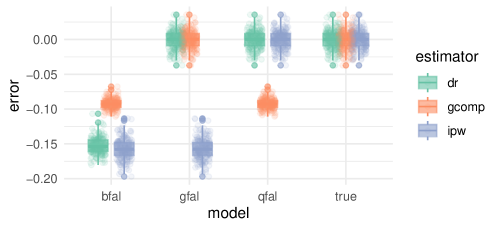
Figure 2: Results of each estimator applied to $nsims=200$ simulated datasets of $nobs=10,000$ each. $bfal$ indicates all models misspecified, $qfal$ only outcomes models misspecified, $gfal$ both selection and treatment models misspecified, and $true$ all models correctly specified.

6 Discussion

This paper introduced an approach to estimating treatment effects in a target population based on DID conducted in a study sample that differs from the target population. Under certain assumptions, some of which may be understood with the aid of causal diagrams, we can identify the PATT, PATE, and PATU. We also propose several estimators of the aforementioned effects in the target population that only require measurement of covariates and/or treatments in the target population, not necessarily outcomes. This approach may be useful when, as is the case in our motivating example involving air nicotine, measurement of outcomes in the target population (in this case, the entire U.S.) may not be feasible, and unobserved confounding is present (in this case, ventilation) but those unobserved confounders do not modify the additive treatment effect. Though our approach assumed the same set of covariates were sufficient for internal and external validity, the methods can easily be adapted to settings where the covariates needed for external validity are a subset of those needed for internal validity. Though our approach has been framed around the problem of transportability (i.e., the study sample is not a subset of target population), our methods can easily be adapted to generalizability problems (when the study sample is nested in the target population). The approach may therefore also prove useful when a select group of jurisdictions (such as states or provinces) implement a policy, but decisions need to made a higher level of organization (such as national governments).

It is important to note that our motivating example was greatly simplified for illustrative purposes; a full analysis to address the motivating question would likely be more complex. For example, one would need to carefully consider how the exclusion criteria may impact the plausibility of assumptions, whether other covariates would need to be measured, and whether differences in building management between public housing in NYC and other areas might violate treatment version irrelevance.

Causal diagrams have rarely been employed to understand identification in DID designs, but have been essential for elucidating the way causal structure impacts generalizability and transportability problems. By employing causal diagrams, we highlighted that the causal structure implied by unmeasured confounding that often motivates DID creates particular complexities for generalizability and transportability. Specifically, we were able to identify transported treatment effects under an assumption that the unmeasured confounders are not additive effect measure modifiers, but not necessarily otherwise.

The validity of an assumption that unmeasured confounders are not additive effect measure modifiers may be difficult to assess in practice. In our example, we possess no a priori substantive information to suggest that the additive effect of a smoking ban on log-transformed air nicotine would be constant according to the building’s level of ventilation (a presumed confounder). This suggests that, when transportability is of interest in DID studies, investigators should measure and adjust for as many potential confounders as possible (even if not formally needed for parallel trends) in order to reduce the number of variables for which we must make homogeneity assumptions. Future work will seek to develop bounds under violations of effect homogeneity along with methods to assess the sensitivity of conclusions to this key assumption.

Appendix A Proof of identification results

A.1 Proof of Theorem 1

First we show identification for the PATT:

$$\mathbb{E}[Y_{1}(1) -Y_{1}(0)|A=1,S=0]=\mathbb{E}\{\mathbb{E}[Y_{1}(1)-Y_{1}(0)|W,U,A=1,S=0]|A=1,S=0\}$$ (iterated expectation)

$$=\mathbb{E}\{\mathbb{E}[Y_{1}(1)-Y_{1}(0)|W,U,A=1,S=1]|A=1,S=0\}$$ (Assumptions 1, 2, 10 & 11)

$$=\mathbb{E}\{\mathbb{E}[Y_{1}(1)-Y_{1}(0)|W,A=1,S=1]|A=1,S=0\}$$ (Assumption 12)

$$=\mathbb{E}(m_{1}(W)-m_{0}(W)|A=1,S=0)$$ (Assumptions 1-5)

Next consider identification of the PATU:

$$\mathbb{E}[Y_{1}(1) -Y_{1}(0)|A=0,S=0]=\mathbb{E}\{\mathbb{E}[Y_{1}(1)-Y_{1}(0)|W,U,A=0,S=0]|A=0,S=0\}$$ (iterated expectation)

$$=\mathbb{E}\{\mathbb{E}[Y_{1}(1)-Y_{1}(0)|W,U,A=0,S=1]|A=0,S=0\}$$ (Assumptions 1, 2, 10 & 11)

$$=\mathbb{E}\{\mathbb{E}[Y_{1}(1)-Y_{1}(0)|W,U,A=1,S=1]|A=0,S=0\}$$ (Assumptions 1, 2, 8 & 9)

$$=\mathbb{E}\{\mathbb{E}[Y_{1}(1)-Y_{1}(0)|W,A=1,S=1]|A=0,S=0\}$$ (Assumption 12)

$$=\mathbb{E}(m_{1}(W)-m_{0}(W)|A=0,S=0)$$ (Assumptions 1-5)

Having identified the PATU and the PATT, the PATE is trivially identified:

$$\mathbb{E}[Y_{1}(1)-Y_{1}(0)|S=0] =\mathbb{E}[\mathbb{E}(Y_{1}(1)-Y_{1}(0)|A,S=0)|S=0]$$

$$=\mathbb{E}[\mathbb{E}(m_{1}(W)-m_{0}(W)|A,S=0)|S=0]$$

$$=\mathbb{E}[m_{1}(W)-m_{0}(W)|S=0]$$

A.2 Identifying the SATE and SATU under additional assumptions

Under Assumptions 8, 9, and 12, the SATE is identified as

$$\mathbb{E}[Y_{1}(1) -Y_{1}(0)|S=1]=\mathbb{E}\{\mathbb{E}[Y_{1}(1)-Y_{1}(0)|W,U,S=1]|S=1\}$$ (iterated expectation)

$$=\mathbb{E}\{\mathbb{E}[Y_{1}(1)-Y_{1}(0)|W,U,A=1,S=1]|S=1\}$$ (Assumptions 8 & 9)

$$=\mathbb{E}\{\mathbb{E}[Y_{1}(1)-Y_{1}(0)|W,A=1,S=1]|S=1\}$$ (Assumption 12)

$$=\mathbb{E}\{m_{1}(W)-m_{0}(W)|S=1\} \quad\text{(Assumptions \ref{asn:noint}-\ref{asn:pt})},$$

and the SATU is identified as:

$$\mathbb{E}[Y_{1}(1) -Y_{1}(0)|A=0,S=1]=\mathbb{E}\{\mathbb{E}[Y_{1}(1)-Y_{1}(0)|W,U,A=0,S=1]|A=0,S=1\}$$ (iterated expectation)

$$=\mathbb{E}\{\mathbb{E}[Y_{1}(1)-Y_{1}(0)|W,U,A=1,S=1]|A=0,S=1\}$$ (Assumptions 8 & 9)

$$=\mathbb{E}\{\mathbb{E}[Y_{1}(1)-Y_{1}(0)|W,A=1,S=1]|A=0,S=1\}$$ (Assumption 12)

$$=\mathbb{E}\{m_{1}(W)-m_{0}(W)|A=0,S=1\}$$ (Assumptions 1-5)

Appendix B Efficient influence function for transported treatment effects

To ease notation, we let $\Delta Y=Y_{1}-Y_{0}.$ We let $P_{n}\{h(O)\}=n^{-1}\sum_{i=1}^{n}h(O_{i})$ denote the sample mean of a function $h(\cdot)$ of the observed data $O$, $P$ dnote the true distribution of the observed data, and $\widehat{P}_{n}$ denote an estimator of the observed data distribution (which may or may not be the empirical distribution). Here we focus on the statistical estimand

$$\psi(a^{*},P) =\mathbb{E}[m_{1}(W)-m_{0}(W)|A=a^{*},S=0]\}$$

$$=\int[m_{1}(z)-m_{0}(w)]f(w|A=a^{*},S=0)dw$$

where we write $\psi(a^{*},P)$ as a function of $P$ to emphasize that it depends on the true observed data distribution.

B.1 Proof of EIF

Theorem 2.

The efficient influence function for $\psi(a^{*})$ is given by

$$D(a^{*},O_{i},P) =\frac{I(A_{i}=1,S_{i}=1)g_{a^{*},0}(W_{i})}{f(A=a^{*},S=0)g_{1,1}(W_{i})}\{\Delta Y_{i}-m_{1}(W_{i})\}-\frac{I(A_{i}=0,S_{i}=1)g_{a^{*},0}(W_{i})}{f(A=a^{*},S=0)g_{0,1}(W_{i})}\{\Delta Y_{i}-m_{0}(W_{i})\}$$

$$\quad\quad+\frac{I(A_{i}=a^{*},S_{i}=0)}{f(A=a^{*},S=0)}\{m_{1}(W_{i})-m_{0}(W_{i})\}-\psi(a^{*})$$

Proof.

NOTE: this proof is somewhat non-rigorous because it appears at times to rely on $W$ being discrete and other times continuous. Plan is to re-rewrite using the approach of Hines et al. [23].

$$IF\{\psi(a^{*},P)\} =\int\bigg{(}IF\{m_{1}(w)\}-IF\{m_{0}(w)\}\bigg{)}f(w|A=a^{*},S=0)dw+\int\{m_{1}(W)-m_{0}(w)\}IF\{f(w|A=a^{*},S=0)\}dw$$

$$=\int\frac{I(A=1,S=1,W=w)}{f(A=1,S=1,W=w)}[\Delta Y-m_{1}(w)]f(w|A=a^{*},S=0)dw$$

$$\quad-\int\frac{I(A=0,S=1,W=w)}{f(A=0,S=1,W=w)}[\Delta Y-m_{0}(w)]f(w|A=a^{*},S=0)dw$$

$$\quad+\int\{m_{1}(w)-m_{0}(w)\}\frac{I(A=a^{*},S=0)}{f(A=a^{*},S=0)}\{I(W=w)-f(w|A=a^{*},S=0)\}dw$$

$$=\frac{I(A=1,S=1)g_{a^{*},0}(W)}{f(A=a^{*},S=0)g_{1,1}(W)}[\Delta Y-m_{1}(W)]-\frac{I(A=0,S=1)g_{a^{*},0}(W)}{f(A=a^{*},S=0)g_{0,1}(W)}[\Delta Y-m_{0}(W)]$$

$$\quad+\frac{I(A=a^{*},S=0)}{f(A=a^{*},S=0)}[m_{1}(W)-m_{0}(W)]-\int\{m_{1}(w)-m_{0}(w)\}f(w|A=a^{*},S=0)dw$$

where the first equality uses the fact that the efficient influence function is a derivative and applies the product rule for derivatives, the second substitutes known influence functions for conditional expectations and conditional densities/probability mass functions, and the third rearranges. ∎

B.2 One-step estimator

Because the efficient influence function for $\psi(a^{*})$ is given by $D(a^{*},O_{i},P)$, a one-step estimator [23] is given by

$$\widehat{\psi}_{dr}(a^{*}) =\psi(a^{*},\widehat{P}_{n})-P_{n}\{D(a^{*},O_{i},\widehat{P}_{n})\}$$

$$=P_{n}\bigg{\{}\frac{I(A=1,S=1)\widehat{g}_{a^{*},0}(W)}{P_{n}(I[A=a^{*},S=0])\widehat{g}_{1,1}(W)}\{\Delta Y-\widehat{m}_{1}(W)\}-\frac{I(A=0,S=1)\widehat{g}_{a^{*},0}(W)}{P_{n}(I[A=a^{*},S=0])\widehat{g}_{0,1}(W)}\{\Delta Y-\widehat{m}_{0}(W)\}$$

$$\quad\quad+\frac{I(A=a^{*},S=0)}{P_{n}(I[A=a^{*},S=0])}\{\widehat{m}_{1}(W)-\widehat{m}_{0}(W)\}\bigg{\}}$$

where $\widehat{P}_{n}=\{\widehat{g}_{a,s},\widehat{m}_{a}\}$ with $\{a,s\}\in\{0,1\}^{2}.$ If $\widehat{P}_{n}$ consists of correctly-specified parametric models, it follows by the central limit theorem that

$$\sqrt{n}[\widehat{\psi}_{dr}(a^{*})-\psi(a^{*})]\xrightarrow{d}N(0,\mathbb{E}[D(a^{*},O,\widehat{P}_{n})^{2}])$$

where $\xrightarrow{d}$ denotes convergence in distribution. Thus, an estimator of the asymptotic variance that is consistent when $\widehat{P}_{n}$ consists of correctly-specified parametric models is given by

$$\widehat{var}[\widehat{\psi}_{dr}(a^{*})]=P_{n}\{D(a^{*},O,\widehat{P}_{n})^{2}\}$$

Appendix C Double robust property of $\widehat{\psi}_{dr}$

In this section, for ease of notation we let $m_{a}\equiv m_{a}(W)$ and $g_{a,s}\equiv g_{a,s}(W)$. First, suppose $\widehat{m}_{a}\xrightarrow{p}m_{a}^{*}$ and $\widehat{g}_{a,s}\xrightarrow{p}g_{a,s}^{*}$, not necessarily assuming $g_{a,s}=g_{a,s}^{*}$ or $m_{a}=m_{a}^{*}$. Using Slutzky’s theorem and continuous mapping theorem we have

$$\widehat{\psi}_{dr}(a^{*}) \xrightarrow{p}\psi^{*}(a^{*})\equiv\mathbb{E}\bigg{\{}\frac{I(A=1,S=1)g_{a^{*},0}^{*}}{f(A=a^{*},S=0)g_{1,1}^{*}}\{\Delta Y-m_{1}^{*}\}-\frac{I(A=0,S=1)g_{a^{*},0}^{*}}{f(A=a^{*},S=0)g_{0,1}^{*}}\{\Delta Y-m_{0}^{*}\}$$

$$\quad\quad\quad+\frac{I(A=a^{*},S=0)}{f(A=a^{*},S=0)}\{m_{1}^{*}-m_{0}^{*}\}\ \bigg{\}}$$

First consider the case where outcome models are correctly specified, so that $m_{a}(w)=m_{a}^{*}(w)$ for all $w\in\mathcal{W}.$ By the linearity property of expectations, we have

$$\psi^{*}(a^{*}) =\mathbb{E}\bigg{\{}\frac{I(A=1,S=1)g_{a^{*},0}^{*}}{f(A=a^{*},S=0)g_{1,1}^{*}}(\Delta Y-m_{1}^{*})\bigg{\}}$$ (C.1)

$$\quad\quad-\mathbb{E}\bigg{\{}\frac{I(A=0,S=1)g_{a^{*},0}^{*}}{f(A=a^{*},S=0)g_{0,1}^{*}}(\Delta Y-m_{0}^{*})\bigg{\}}$$ (C.2)

$$\quad\quad+\mathbb{E}\bigg{\{}\frac{I(A=a^{*},S=0)}{f(A=a^{*},S=0)}(m_{1}^{*}-m_{0}^{*})\bigg{\}}$$ (C.3)

Under $m_{a}=m_{a}^{*},$ we have

$$(\ref{eq:dr1}) =\mathbb{E}\bigg{\{}\frac{I(A=1,S=1)g_{a^{*},0}^{*}}{f(A=a^{*},S=0)g_{1,1}^{*}}(\mathbb{E}[\Delta Y|A=1,S=1,W]-m_{1})\bigg{\}}$$

$$=0$$

Likewise, $(\ref{eq:dr2})=0.$ Therefore, $\psi^{*}(a^{*})=\mathbb{E}\bigg{\{}\frac{I(A=a^{*},S=0)}{f(A=a^{*},S=0)}(m_{1}-m_{0})\bigg{\}}=\mathbb{E}[m_{1}-m_{0}|A=a^{*},S=0]=\psi(a^{*}).$ Moreover, because (C.3) is the probability limit of the g-computation estimator, we have that $\widehat{\psi}_{gcomp}(a^{*})\xrightarrow{p}\psi(a^{*})$ whenever $\widehat{m}_{a}\xrightarrow{p}m_{a}.$

Next, consider the case where treatment and selection models are correctly specified, so that $g_{a,s}(w)=g_{a,s}^{*}(w)$ for all $w\in\mathcal{W}$. Rearranging we have

$$\psi^{*}(a^{*}) =\mathbb{E}\bigg{\{}\bigg{(}\frac{I(A=1,S=1)g_{a^{*},0}^{*}}{f(A=a^{*},S=0)g_{1,1}^{*}}-\frac{I(A=0,S=1)g_{a^{*},0}^{*}}{f(A=a^{*},S=0)g_{0,1}^{*}}\bigg{)}\Delta Y\bigg{\}}$$ (C.4)

$$\quad+\mathbb{E}\bigg{\{}\bigg{(}\frac{I(A=0,S=1)g_{a^{*},0}^{*}}{f(A=a^{*},S=0)g_{0,1}^{*}}-\frac{I(A=1,S=0)}{f(A=a^{*},S=0)}\bigg{)}m_{0}^{*}\bigg{\}}$$ (C.5)

$$\quad-\mathbb{E}\bigg{\{}\bigg{(}\frac{I(A=1,S=1)g_{a^{*},0}^{*}}{f(A=a^{*},S=0)g_{1,1}^{*}}-\frac{I(A=a^{*},S=0)}{f(A=a^{*},S=0)}\bigg{)}m_{1}^{*}\bigg{\}}$$ (C.6)

Since $g_{a,s}^{*}=g_{a,s}$, we have

$$(\ref{eq:dr4}) =\mathbb{E}\bigg{\{}\bigg{(}\frac{I(A=1,S=1)f(A=a^{*},S=0|W)}{f(A=a^{*},S=0)f(A=1,S=1|W)}-\frac{I(A=0,S=1)f(A=a^{*},S=0|W)}{f(A=a^{*},S=0)f(A=0,S=1|W)}\bigg{)}\Delta Y\bigg{\}}$$

$$=\mathbb{E}\bigg{\{}\frac{I(A=1,S=1)f(A=a^{*},S=0|W)}{f(A=a^{*},S=0)f(A=1,S=1|W)}m_{1}(W)-\frac{I(A=0,S=1)f(A=a^{*},S=0|W)}{f(A=a^{*},S=0)f(A=0,S=1|W)}m_{0}(W)\bigg{\}}$$

$$=\mathbb{E}\bigg{\{}\frac{\mathbb{E}[I(A=1,S=1)|W]f(A=a^{*},S=0|W)}{f(A=a^{*},S=0)f(A=1,S=1|W)}m_{1}(W)-\frac{E[I(A=0,S=1)|W]f(A=a^{*},S=0|W)}{f(A=a^{*},S=0)f(A=0,S=1|W)}m_{0}(W)\bigg{\}}$$

$$=\mathbb{E}\bigg{\{}\frac{f(A=a^{*},S=0|W)}{f(A=a^{*},S=0)}[m_{1}(W)-m_{0}(W)]\bigg{\}}$$

$$=\mathbb{E}\bigg{\{}\frac{I(A=a^{*},S=0)}{f(A=a^{*},S=0)}[m_{1}(W)-m_{0}(W)]\bigg{\}}$$

$$=\psi(a^{*})$$

$$(\ref{eq:dr5}) =\mathbb{E}\bigg{\{}\bigg{(}\frac{\mathbb{E}[I(A=0,S=1)|W]f(A=a^{*},S=0|W)}{f(A=a^{*},S=0)f(A=0,S=1|W)}-\frac{I(A=a^{*},S=0)}{f(A=a^{*},S=0)}\bigg{)}m_{0}^{*}\bigg{\}}$$

$$=\mathbb{E}\bigg{\{}\bigg{(}\frac{f(A=a^{*},S=0|W)}{f(A=a^{*},S=0)}-\frac{I(A=a^{*},S=0)}{f(A=a^{*},S=0)}\bigg{)}m_{0}^{*}\bigg{\}}$$

$$=0$$

Likewise, (C.6)=$\mathbb{E}\bigg{\{}\bigg{(}\frac{f(A=a^{*},S=0|W)}{f(A=a^{*},S=0)}-\frac{I(A=a^{*},S=0)}{f(A=a^{*},S=0)}\bigg{)}m_{1}^{*}\bigg{\}}=0.$ Thus if $\widehat{g}_{a,s}(w)\xrightarrow{p}g_{a,s}(w)$, $\widehat{\psi}_{dr}(a^{*})\xrightarrow{p}\psi(a^{*}).$ Moreover, because (C.4) is the probability limit of the IOW estimator, we have that $\widehat{\psi}_{IOW}(a^{*})\xrightarrow{p}\psi(a^{*})$ whenever $\widehat{g}_{a,s}\xrightarrow{p}g_{a,s}$.

References

- [1] Michael Lechner “The estimation of causal effects by difference-in-difference methods” In Foundations and Trends® in Econometrics 4.3 Now Publishers, Inc., 2011, pp. 165–224
- [2] Jonathan Roth, Pedro HC Sant’Anna, Alyssa Bilinski and John Poe “What’s trending in difference-in-differences? A synthesis of the recent econometrics literature” In Journal of Econometrics Elsevier, 2023
- [3] Guido W Imbens and Jeffrey M Wooldridge “Recent developments in the econometrics of program evaluation” In Journal of economic literature 47.1 American Economic Association, 2009, pp. 5–86
- [4] Tamar Sofer et al. “On negative outcome control of unobserved confounding as a generalization of difference-in-differences” In Statistical science: a review journal of the Institute of Mathematical Statistics 31.3 NIH Public Access, 2016, pp. 348
- [5] Catherine R Lesko et al. “Generalizing study results: a potential outcomes perspective” In Epidemiology (Cambridge, Mass.) 28.4 NIH Public Access, 2017, pp. 553
- [6] Judea Pearl and Elias Bareinboim “External Validity: From Do-Calculus to Transportability Across Populations” In Statistical Science 29.4, 2014, pp. 579–595
- [7] Stephen R Cole and Elizabeth A Stuart “Generalizing evidence from randomized clinical trials to target populations: the ACTG 320 trial” In American journal of epidemiology 172.1 Oxford University Press, 2010, pp. 107–115
- [8] Daniel Westreich et al. “Transportability of trial results using inverse odds of sampling weights” In American journal of epidemiology 186.8 Oxford University Press, 2017, pp. 1010–1014
- [9] Kara E Rudolph, Nicholas T Williams, Elizabeth A Stuart and Ivan Diaz “Efficiently transporting average treatment effects using a sufficient subset of effect modifiers” In arXiv preprint arXiv:2304.00117, 2023
- [10] Joel B Greenhouse et al. “Generalizing from clinical trial data: a case study. The risk of suicidality among pediatric antidepressant users” In Statistics in medicine 27.11 Wiley Online Library, 2008, pp. 1801–1813
- [11] Elizabeth A Stuart, Catherine P Bradshaw and Philip J Leaf “Assessing the generalizability of randomized trial results to target populations” In Prevention Science 16 Springer, 2015, pp. 475–485
- [12] Bénédicte Colnet et al. “Causal inference methods for combining randomized trials and observational studies: a review” In arXiv preprint arXiv:2011.08047, 2020
- [13] Judea Pearl “Causal diagrams for empirical research” In Biometrika 82.4 Oxford University Press, 1995, pp. 669–688
- [14] Judea Pearl and Elias Bareinboim “Transportability of causal and statistical relations: A formal approach” In Proceedings of the AAAI Conference on Artificial Intelligence 25.1, 2011, pp. 247–254
- [15] Ellen C Caniglia and Eleanor J Murray “Difference-in-difference in the time of cholera: a gentle introduction for epidemiologists” In Current epidemiology reports 7 Springer, 2020, pp. 203–211
- [16] Jonathan Roth and Pedro HC Sant’Anna “When is parallel trends sensitive to functional form?” In Econometrica 91.2 Wiley Online Library, 2023, pp. 737–747
- [17] Issa J Dahabreh et al. “Extending inferences from a randomized trial to a new target population” In Statistics in medicine 39.14 Wiley Online Library, 2020, pp. 1999–2014
- [18] James J Heckman, Hidehiko Ichimura and Petra E Todd “Matching as an econometric evaluation estimator: Evidence from evaluating a job training programme” In The review of economic studies 64.4 Wiley-Blackwell, 1997, pp. 605–654
- [19] Alberto Abadie “Semiparametric difference-in-differences estimators” In The review of economic studies 72.1 Wiley-Blackwell, 2005, pp. 1–19
- [20] Brantly Callaway, Andrew Goodman-Bacon and Pedro HC Sant’Anna “Difference-in-differences with a continuous treatment” In arXiv preprint arXiv:2107.02637, 2021
- [21] Elle Anastasiou et al. “Long-term trends in secondhand smoke exposure in high-rise housing serving low-income residents in New York City: three-year evaluation of a federal smoking ban in public housing, 2018–2021” In Nicotine and Tobacco Research 25.1 Oxford University Press US, 2023, pp. 164–169
- [22] Thomas S Richardson and James M Robins “Single world intervention graphs (SWIGs): A unification of the counterfactual and graphical approaches to causality” In Center for the Statistics and the Social Sciences, University of Washington Series. Working Paper 128.30 Citeseer, 2013, pp. 2013
- [23] Oliver Hines, Oliver Dukes, Karla Diaz-Ordaz and Stijn Vansteelandt “Demystifying statistical learning based on efficient influence functions” In The American Statistician 76.3 Taylor & Francis, 2022, pp. 292–304