Abstract

Neural Temporal Point Processes (TPPs) have emerged as the primary framework for predicting sequences of events that occur at irregular time intervals, but their sequential nature can hamper performance for long-horizon forecasts. To address this, we introduce a novel approach that incorporates a diffusion generative model. The model facilitates sequence-to-sequence prediction, allowing multi-step predictions based on historical event sequences. In contrast to previous approaches, our model directly learns the joint probability distribution of types and inter-arrival times for multiple events. This allows us to fully leverage the high dimensional modeling capability of modern generative models. Our model is composed of two diffusion processes, one for the time intervals and one for the event types. These processes interact through their respective denoising functions, which can take as input intermediate representations from both processes, allowing the model to learn complex interactions. We demonstrate that our proposal outperforms state-of-the-art baselines for long-horizon forecasting of TPP.

1 INTRODUCTION

Figure 1: Visualization of the cross-diffusion generating process for 15 examples sequences of the Stackoverflow dataset. The colors indicates the different categories. We start by generating noisy sequences ($t=T$). Once we reach the end of the denoising process ($t=0$), we have recovered sequences similar to the ground truth sequences.

Predicting sequences of events has many practical applications, such as forecasting purchase times, scheduling based on visitor arrival times, and modeling transaction patterns or social media activity. This specific problem requires a dedicated model because it involves the complex task of jointly modeling two challenging data types: strictly positive continuous data for inter-arrival times and categorical data representing event types.

Early works relied on principled intensity-based models for temporal point processes, such as the Hawkes process (Liniger,, 2009). This modelling choice comes with many advantages, including its interpretability — it specifies the dynamics between events in the sequence explicitly. As a result, many early efforts targeted integrating deep learning methods within the intensity framework to improve its modeling power (Mei and Eisner,, 2017; Zuo et al.,, 2020; Yang et al.,, 2022).

Although not highly restrictive, intensity-based models do have limits on the flexibility of their structure. As generative modeling research has developed, TPP models have gradually moved away from the intensity parameterization, with more flexible specifications allowing them to use the full potential of recent generative models (Shchur et al., 2020a, ; Gupta et al.,, 2021; Lin et al.,, 2022).

Until recently, almost all of the research effort has focused on next event forecasting. In (Xue et al.,, 2022; Deshpande et al.,, 2021), attention has turned to a longer horizon, with the goal being forecasting of multiple future events. The recent proposals are still autoregressive, so they can suffer from error propagation, but they are paired with additional modules that strive to mitigate this.

Our proposal goes a step further by directly generating a sequence of events. We build on recent advances in generative models, exploiting their impressive high-dimensionality modeling capabilities. Consequently, our model can capture intricate interactions within the sequence of events between arrival times and event types. The innovation of our approach is highlighted in Fig. 1. We use coupled denoising diffusion processes to learn the probability distribution of the event sequences. One is a categorical diffusion process; the other is real-valued. The interaction of the neural networks that model the reverse processes allows us to learn dependencies between event type and interarrival time. A visualization of the generation process of our approach can be viewed in Figure 1.

Our approach significantly outperforms existing baselines for long-term forecasting, while also improving efficiency. The analysis we present provides insights into how the model achieves this; we show that our model can capture more complex correlation structures and that it is better at predicting distant events.

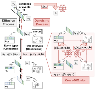
Figure 2: Architectural overview of our model CDiff. We employ two interacting denoising diffusion processes, one categorical and one real-valued, to model the high-dimensional event sequences. The neural networks modeling the reverse diffusion steps interact, allowing them to learn dependencies between event types and interarrival times. Generating an entire sequence at once avoids the error propagation that can plague autoregressive models.

2 PROBLEM STATEMENT

Consider a sequence of events denoted by $\mathbf{s}=\{(x_{i},e_{i})\}_{1\leq i\leq T}$, where $x_{i}\in[0,\infty)$ corresponds to the time interval between the events $e_{i}$ and $e_{i-1}$, and the event $e_{i}$ belongs to one of $K$ categories: $e_{i}\in\mathcal{C},|\mathcal{C}|=K$. We observe the start of a sequence (the context) $\mathbf{s}_{c}=\{(x_{i},e_{i})\}_{1\leq i\leq I}$ (or $\mathbf{x}_{c}=[x_{1},...,x_{I}]$ and $\mathbf{e}_{c}=[e_{1},...,e_{I}]$ in vector form) with $I<T$, and the goal is to forecast the remaining events.

Next $N$ events forecasting

In this setting, the task is to predict the following $N$ events in the sequence $\mathbf{s}_{u}$: $\mathbf{x}_{u}=[x_{I+1},...,x_{I+N}]$ and $\mathbf{e}_{u}=[e_{I+1},...,e_{I+N}]$. We also consider a slightly different setting: interval forecasting where we focus on time intervals rather than number of events. We include the description of that setting, as well as the metrics and methodology in the Appendix 9.1.

3 RELATED WORK

We now briefly review and discuss the relevant TPP modelling and forecasting literature.

Hawkes-based methods.

Early works on the TPP forecasting problem focused on single-event prediction (Next $N{=}1$ event forecasting) and adopted intensity distributions (Rasmussen,, 2011) as the framework for their solutions. One well-known example of such a parameterization is the multivariate Hawkes Process (MHP) (Liniger,, 2009). This was used as the basis for multiple models (Du et al.,, 2016; Mei and Eisner,, 2017; Zuo et al.,, 2020; Yang et al.,, 2022). Other approaches deviated from the MHP but retained the intensity function, either by incorporating graph learning (Zhang et al.,, 2021), non-parametric methods (Pan et al.,, 2021) or through a meta-learning framework (Bae et al.,, 2023). Despite its simplicity, the intensity parameterization has limitations, leading some researchers to focus on enhancing its efficiency (Shchur et al., 2020b, ; Nickel and Le,, 2020) and expressiveness (Omi et al.,, 2019)

Non-Hawkes methods

Recognizing the limited expressiveness of intensity formulations, some works have opted to move away from them. Shchur et al., 2020a use a log-normal distribution paired with normalising flows. A similar approach is taken by Gupta et al., (2021, 2022) for the different setting of missing data.  Lin et al., (2022) explore multiple conditional generative models for time forecasting including diffusion, variational inference, Generative Adversarial Networks (GANs), and normalizing flows. Each of these proposed models is presented within a unified framework, in which type prediction is modelled independently from time prediction.

Although these works do leverage recent advances in generative modeling, they limit themselves to only modelling a single upcoming event ($N=1$). As a result, they do not exploit the models’ impressive capability to model complex high dimensional data. In addition, modelling type and interarrival time independently is undesirable given that different event types can often be associated with very different arrival patterns.

Long horizon forecasting

The previously mentioned methods address only the single-event forecasting task. In contrast, Xue et al., (2022) and Deshpande et al., (2021) consider the problem of long horizon forecasting. Xue et al., (2022) generate multiple candidate prediction sequences for the same forecasting task and introduce a selection module that aims to learn to select the best candidate. Deshpande et al., (2021) introduce a hierarchical architecture and use a ranking objective that encourages better prediction of the correct number of events in a given interval.

Even though these works explicitly target long horizon forecasting, their generation mechanisms are still sequential. The techniques introduce components to try to mitigate the problem of error propagation in sequential models, but fundamentally they still only learn a model for $p(\{e_{h+1},x_{h+1}\}|\{e_{i},x_{i}\}_{i\leq h})$. As a result, the algorithms retain the core limitations of one-step ahead autoregressive forecasting.

4 METHODOLOGY

Model Overview

Our proposal is to tackle the multi-event forecasting problem by directly modelling a complete sequence of $N$ events. We therefore frame our problem as learning the conditional distribution $P(S_{u}|\mathbf{s}_{c})$ where $S_{u}=Eu,X_{u}$ and introduce our Cross-Diffusion (CDiff) model, which comprises two interacting diffusion processes.

In a nutshell, we diffuse simultaneously both the time intervals and the event types of the target sequence of events: we gradually add Gaussian noise to the time intervals and uniform categorical noise to the types ${S_{0},S_{1},\dots,S_{T}}$ until only noise remains in $S_{T}$. $S_{0}$ denotes the target sequence $S_{u}$. During training, we learn denoising distributions $p_{\theta}(S_{t-1}|S_{t},\mathbf{s}_{c})$ that can undo each of the noise-adding steps. Our denoising functions are split in two, but interact with each other, which is why we call our model “cross-diffusion.” After training, we can sample from $P(S_{u}|\mathbf{s}_{c})$ by sampling noise $S_{T}$, then gradually reversing the chain by sampling from $p_{\theta}(S_{t-1}|S_{t},\mathbf{s}_{c})$ until we recover $S_{0}$. A high-level summary of our approach is illustrated in Figure 2. The specifics of the model and its training are provided in the subsequent sections.

4.1 Model Details

A TPP model can generally be divided into two components (Lin et al.,, 2022): 1) the encoder of the variable length context $\mathbf{s}_{c}$; and 2) the generative model of the future events. We focus on the latter and adopt the transformer-based context encoder proposed by Xue et al., (2022), in order to generate a fixed-dimensional context representation denoted as $\bm{h}=f_{\theta}(\mathbf{s}_{c})$.

We first apply a Box-Cox transformation to the inter-arrival time values to transition from the strictly positive continuous domain to the more convenient unrestricted real space. This allows us to model the variables with Gaussian distributions in the diffusion process. Details can be found in the Appendix 9.5.

Even though the target distribution consists of a combination of categorical and continuous variables, we can define a single diffusion process for it. To achieve this, we begin by defining a forward/noisy process that introduces $T$ new random variables, which are noisier versions of the sequence, represented by $S_{0}=(X_{0},E_{0})$:

$$q(X_{1:T},E_{1:T}|X_{0},E_{0})=\prod^{T}_{t=1}q(X_{t},E_{t}|X_{t-1},E_{t-1}).$$ (1)

The learning task for a diffusion model consists of learning the inverse denoising process, by learning the intermediate distributions $p_{\theta}(S_{t-1}|S_{t},\mathbf{s}_{c})$. The log likelihood of the target distribution $\log q(S_{0})$ can be obtained through marginalization over this denoising process. Following the conventional diffusion model setup (Ho et al.,, 2020), this marginalization can be approximated as:

$$\log q(S_{0}) \geq\mathbb{E}_{q(S_{0})}\Big{[}\log p_{\theta}(S_{0}|S_{1},\mathbf{s}_{c})$$

$$-KL(q(S_{T}S_{0})||q(S_{T}))$$

$$-\sum^{T}_{t=2}KL\Big{(}q(S_{t-1}|S_{t,0})||p_{\theta}(S_{t-1}|S_{t},\mathbf{s}_{c})\Big{)}\Big{]}.$$ (2)

Hence, we can summarize the generative diffusion model approach as follows: by minimizing the KL-divergences between the learned distributions $p_{\theta}(S_{t-1}|S_{t},\mathbf{s}_{c})$ and the noisy distributions $q(S_{t-1}|S_{t,0})$ at each $t$, we maximize the log likelihood of our target $\log q(S_{0})$ .

Cross-diffusion for modeling sequences of event

As $X_{u}$ and $E_{u}$ are in different domains, we cannot apply a standard noise function to $q(X_{t},E_{t}|X_{t-1},E_{t-1})$. Instead, we factorize the noise-inducing distribution $q(S_{t}|S_{t-1})=q(X_{t}|X_{t-1})q(E_{t}|E_{t-1})$. It is important to stress that this independence is only imposed on the forward (noise-adding) process. We are not assuming any independence in $q(S_{0})$ and our reverse diffusion process, described below, allows us to learn the dependencies. Given an increasing variance schedule $\{\beta_{1},\dots,\beta_{T}\}$, the forward process is defined as:

$$q(S_{t}|S_{t-1})= q(X_{t}|X_{t-1})q(E_{t}|E_{t-1}),$$ (3)

$$q(X_{t}|X_{t-1})= \mathcal{N}(X_{t};\sqrt{1-\beta_{t}}x_{X-1},\beta_{t}\mathbf{I}),$$ (4)

$$q(E_{t}|E_{t-1})= Cat(X_{y};(1-\beta_{t})X_{t-1}+\beta_{t}/K),$$ (5)

$$q(X_{T})= \mathcal{N}(X_{T};0,\mathbf{I}),$$ (6)

$$q(E_{T})= Cat(X_{T};1/K),$$ (7)

Here, $Cat(;p)$ denotes the categorical distribution with parameter $p$.

Next, we have to define our denoising process $p_{\theta}(S_{t-1}|S_{t})$. We can express the joint distribution as:

$$p_{\theta}(S_{t-1}|S_{t},\mathbf{s}_{c})= p_{\theta}(X_{t-1}|S_{t},E_{t-1},\mathbf{s}_{c})p_{\theta}(E_{t-1}|S_{t},\mathbf{s}_{c}),$$ (8)

where we choose to fix $\sigma_{t}=\beta_{t}$, and

$$p_{\theta}(E_{t-1}|S_{t})\triangleq Cat(E_{t-1};\pi_{\theta}(X_{t},E_{t},t,\mathbf{s}_{c})),$$ (9)

$$p_{\theta}(X_{t-1}|S_{t},E_{t-1})\triangleq \mathcal{N}(X_{t-1};\mu_{\theta}(X_{t},E_{t-1},t,\mathbf{s}_{c}),\sigma_{t}).$$ (10)

With the presented approach, during denoising, we first sample event types, and then conditioned on the sampled event types, we sample inter-arrival times. We can also choose to do the reverse. A sensitivity study in the Appendix 9.8 shows that this choice has a negligible effect on performance.

This can be viewed as two denoising processes that interact with each other through $\mu_{\theta}$ and $\pi_{\theta}$. One models the inter-arrival times (Gaussian) and one models the event types (Categorical).

We follow the standard parametrization for $\mu_{\theta}(\mathbf{x}_{t},\mathbf{e}_{t-1},t,\mathbf{s}_{c})$ and $\pi_{\theta}(\mathbf{x}_{t},\mathbf{e}_{t},t,\mathbf{s}_{c})$ from (Ho et al.,, 2020; Hoogeboom et al.,, 2021):

$$\mu_{\theta}(\mathbf{x}_{t},\mathbf{e}_{t-1},t,\mathbf{s}_{c})=\frac{1}{\sqrt{\alpha_{t}}} \bigg{(}\mathbf{x}_{t}-\frac{\beta_{t}\epsilon_{\theta}(\mathbf{x}_{t},\mathbf{e}_{t-1},t,\mathbf{s}_{c})}{\sqrt{1-\bar{\alpha}_{t}}}\bigg{)},$$ (11)

$$\pi_{\theta}(\mathbf{x}_{t},\mathbf{e}_{t},t,\mathbf{s}_{c})= \tilde{\bm{\theta}}/\sum^{\mathrm{K}}_{k=1}\tilde{\bm{\theta}}_{k},$$ (12)

$$\tilde{\bm{\theta}}= \bm{\theta}(\phi_{\theta}(\mathbf{e}_{t},\mathbf{x}_{t},t,\mathbf{s}_{c})),$$ (13)

$$\bm{\theta}(\mathbf{e})=[\alpha_{t}\mathbf{e}_{t}+\frac{(1-\alpha_{t})}{K}]\odot [\bar{\alpha}_{t-1}\mathbf{e}+\frac{(1-\bar{\alpha}_{t-1})}{K}]$$ (14)

where $\odot$ denotes the Hadamard product, $\alpha_{t}=1-\beta_{t}$ and $\bar{\alpha}_{t}=\prod_{i\leq t}\alpha_{i}$. We define the posterior distribution of the multinomial forward diffusion process as:

$$q(\mathbf{e}_{t-1}|\mathbf{e}_{t},\mathbf{e}_{0}) =Cat(\mathbf{e}_{t-1}|\bar{\bm{\theta}}_{\text{post}}(\mathbf{e}_{t},\mathbf{e}_{0}))$$ (15)

where ${\bar{\bm{\theta}}_{\text{post}}}={\bm{\theta}}(\mathbf{e}_{0})/\sum^{\mathrm{K}}_{k=1}{\bm{\theta}}_{k}(\mathbf{e}_{0})$. Hence, the learnable components of CDiff are $\epsilon_{\theta},\phi_{\theta}$ and $f_{\theta}$. In our experiments, we use transformer-based networks that we describe in Section 5.4.

With a trained model $p_{\theta}(S^{0}|\mathbf{s}_{c})$, given a context sequence $\mathbf{s}_{c}$, we can generate samples of the next $N$ events, $\hat{\mathbf{s}}^{0}\sim p_{\theta}(S^{0}|\mathbf{s}_{c})$. To form the final predicted forecasting sequence $\hat{\mathbf{s}}_{u}$, we generate multiple samples, calculate the average time intervals, and set the event types to the majority types. With an abuse of notation, we denote this averaging of sequences as $\hat{\mathbf{s}}_{u}\triangleq\frac{1}{A}\sum^{A}_{a=1}\hat{\mathbf{s}}_{a}^{0},\quad\hat{\mathbf{s}}_{a}^{0}\sim p_{\theta}(S^{0}|\mathbf{s}_{c})$.

4.2 Optimization

The log-likelihood objective is provided in Equation (2). We can separate the objective for the joint $q(S_{0})$ into standard optimization terms of either continuous or categorical diffusion using Equation (8).

Starting with the first log term, we separate it as:

$$\mathbb{E}_{q(S_{0})}\Big{[}\log p_{\theta}(S_{0}|S_{1},\mathbf{s}_{c})\Big{]}$$

$$\approx\sum^{M}_{j=1}\log p_{\theta}(\mathbf{x}^{j}_{0}|\mathbf{x}^{j}_{1},\hat{\mathbf{e}}^{j}_{0},\mathbf{s}^{j}_{c})+\log p_{\theta}(\mathbf{e}^{j}_{0}|\mathbf{x}^{j}_{1},\mathbf{e}^{j}_{1},\mathbf{s}^{j}_{c}),$$ (16)

with $\mathbf{e}^{j}_{1}\sim q(E_{1}|\mathbf{e}_{0}^{j})$, $\mathbf{x}^{j}_{1}\sim q(X_{1}|\mathbf{x}_{0}^{j})$ and $\hat{\mathbf{e}}^{j}_{0}{\sim}p_{\theta}(E_{0}|\mathbf{x}^{j}_{1},\mathbf{e}^{j}_{1},\mathbf{s}^{j}_{c})$.

Next, we split the individual KL terms from (2) similarly:

$$\mathbb{E}_{q(S_{0})}\Big{[}KL\Big{(}q(S_{t-1}|S_{t,0})||p_{\theta}(S_{t-1}|S_{t},\mathbf{s}_{c})\Big{)}\Big{]}=$$ (17)

$$\mathbb{E}_{q(S_{0})}\Big{[}KL\Big{(}q(X_{t-1}|X_{t,0})||p_{\theta}(X_{t-1}|S_{t},E_{t-1},\mathbf{s}_{c})\Big{)}\Big{]}$$ (18)

$$+ \mathbb{E}_{q(S_{0})}\Big{[}KL\Big{(}q(E_{t-1}|E_{t,0})||p_{\theta}(E_{t-1}|S_{t},\mathbf{s}_{c})\Big{)}\Big{]}.$$ (19)

We can therefore apply the typical optimization techniques of either continuous and categorical diffusion on each term. These are given by:

$$\mathbb{E}_{q(S_{0})} \Big{[}KL\Big{(}q(E_{t-1}|E_{t,0})||p_{\theta}(E_{t-1}|S_{t},\mathbf{s}_{c})\Big{)}\Big{]}$$ (20)

$$\approx -\sum^{M}_{j=1}\sum_{k}\bar{\bm{\theta}}_{\text{post}}(\mathbf{e}^{j}_{t},\mathbf{e}^{j}_{0})_{k}\cdot\log\frac{\bar{\bm{\theta}}_{\text{post}}(\mathbf{e}^{j}_{t},\mathbf{e}^{j}_{0})_{k}}{\pi_{\theta}(\mathbf{x}^{j}_{t},\mathbf{e}^{j}_{t},t,\mathbf{s}^{j}_{c})_{k}}$$ (21)

with $\mathbf{e}^{j}_{t}\sim q(E_{t}|\mathbf{e}_{0}^{j})$, $\mathbf{x}^{j}_{t}\sim q(X_{t}|\mathbf{x}_{0}^{j})$ for the events variables, and:

$$\mathbb{E}_{q(S_{0})} \Big{[}KL\Big{(}q(X_{t-1}|X_{t,0})||p_{\theta}(X_{t-1}|S_{t},E_{t-1},\mathbf{s}_{c})\Big{)}\Big{]}$$ (22)

$$\approx -\sum^{M}_{j=1}\|\epsilon-\epsilon_{\theta}(\sqrt{\bar{\alpha}_{t}}\mathbf{x}^{j}_{0}+\sqrt{1-\bar{\alpha}_{t}}\epsilon,t,\hat{\mathbf{e}}^{j}_{t-1},\mathbf{s}^{j}_{c})\|^{2}$$ (23)

with $\mathbf{e}^{j}_{t}\sim q(E_{t}|\mathbf{e}_{0}^{j})$, $\mathbf{x}^{j}_{t}\sim q(X_{t}|\mathbf{x}_{0}^{j})$, $\hat{\mathbf{e}}^{j}_{t-1}\sim p_{\theta}(E_{t-1}|\mathbf{x}^{j}_{t},\mathbf{e}^{j}_{t},\mathbf{s}^{j}_{c})$ and $\epsilon\sim\mathcal{N}(0,1)$ for the continuous interarrival time variables.

Our final objective is hence given by:

$$\mathcal{L}=\sum^{M}_{j=1} \Big{(}\log p_{\theta}(\mathbf{x}^{j}_{0}|\mathbf{x}^{j}_{1},\hat{\mathbf{e}}^{j}_{0},\mathbf{s}^{j}_{c})\log p_{\theta}(\mathbf{e}^{j}_{0}|\mathbf{x}^{j}_{1},\mathbf{e}^{j}_{1},\mathbf{s}^{j}_{c})$$ (24)

$$-\sum^{T}_{t=2} \Big{(}\|\epsilon-\epsilon_{\theta}(\sqrt{\bar{\alpha}_{t}}\mathbf{x}^{j}_{0}+\sqrt{1-\bar{\alpha}_{t}}\epsilon,t,\hat{\mathbf{e}}^{j}_{t-1},\mathbf{s}^{j}_{c})\|^{2}$$ (25)

$$+ \sum^{K}_{k=1}\bar{\bm{\theta}}_{\text{post}}(\mathbf{e}^{j}_{t},\mathbf{e}^{j}_{0})_{k}\cdot\log\frac{\bar{\bm{\theta}}_{\text{post}}(\mathbf{e}^{j}_{t},\mathbf{e}^{j}_{0})_{k}}{\pi_{\theta}(\mathbf{x}^{j}_{t},\mathbf{e}^{j}_{t},t,\mathbf{s}^{j}_{c})_{k}}\Big{)}\Big{)}.$$ (26)

Finally, we adhere to the common optimization approach used in diffusion models and optimize only one of the diffusion timestep terms per sample instead of the entire sum. The timestep is selected by uniformly sampling $t\sim U(0,T)$. For sampling, we employ the algorithm from (Song et al.,, 2021) for accelerating the sampling. More details are included in Appendix 9.7.

5 EXPERIMENTS

In our experiments, we set $N=20$ (we also include results for $N=5,10$). For each of the sequences in the dataset $\mathcal{D}=\{\mathbf{s}^{j}\}^{M}_{j=1}$, we set the last $N$ events as $\mathbf{s}_{u}$ and set all the remaining starting events as the context $\mathbf{s}_{c}$. The means and standard deviations for all of our results are computed over 10 trials. We train for a maximum of 500 epochs and report the best trained model based on the result of the validation set. Hyperparameter selection is made using the Tree-Structured Parzen Estimator hyperparameter search algorithm from Bergstra et al., (2011). To avoid numerical error when applying the Box-Cox transformation (Tukey,, 1957) to the $x$ values, we first add 1e-7 to all the time values and scale them by $100$.

5.1 Datasets

We use four real-world datasets: Taobao (Alibaba,, 2018), which tracks user clicks made on a website; Taxi (Whong,, 2014), which contains trips to neighborhood made by taxi drivers; StackOverflow (Leskovec and Krevl,, 2014), which tracks the history of a post on stackoverflow; and Retweet (Zhou et al.,, 2013), which tracks the user interactions on social media posts. Our synthetic dataset is generated from a Hawkes model. We follow Xue et al., (2022) for the train/val/test splits, which we report in the Appendix 9.4, with additional details on the datasets.

5.2 Baselines

We compare our CDiff model with $4$ state-of-the-art baselines for event sequence modeling. When available, we use the reported hyperparameters for each experiment, else we follow hyperparameter tuning procedure (See 9.6).

• Neural Hawkes Process (NHP) (Mei and Eisner,, 2017) is a Hawkes-based model that learns parameters with a continuous LSTM. It is the state-of-the-art (SOTA) for RNN-based Hawkes processes.

• Attentive Neural Hawkes Process (AttNHP) (Yang et al.,, 2022) is a Hawkes-based model that integrates attention mechanisms. It is the SOTA for single event forecasting.

• Dual-TPP(Deshpande et al.,, 2021): Dual-TPP uses RMTPP (Du et al.,, 2016) as a based model. It targets long horizon forecasting by jointly learning a distribution of the count of events in segmented time intervals.

• HYPRO (Xue et al.,, 2022) is the SOTA for multi-event/long horizon forecasting. It uses AttNHP as a base model, but includes a module that selects the best multi-event sequences generated.

5.3 Evaluation Metrics

Assessing long horizon performance is challenging as we have two types of values in $\mathbf{s}_{u}$ (categorical and continuous). Therefore, we report both an Optimal Transport Distance metric (OTD) that can directly compare $\mathbf{s}_{u}$ and $\hat{\mathbf{s}}_{u}$ alongside other metrics that either assess the type forecasting $\hat{\mathbf{e}}_{u}$ or the time interval forecasting $\hat{\mathbf{x}}_{u}$.

$OTD$: We use the optimal transport distance for comparing sequence of events proposed by (Mei et al.,, 2019). It is defined as the minimum cost of editing a predicted event sequence $\hat{\mathbf{s}}_{u}$ into the ground truth $\mathbf{s}_{u}$ $L(\hat{\mathbf{s}}_{u},\mathbf{s}_{u})$. To accomplish this edit, it must identify the best alignment – a one-to-one partial matching $\mathbf{a}$ – of the events in the two sequences. We use the algorithm from (Mei et al.,, 2019) to find this alignment, and report the average $OTD$ values when using various deletion/insertion cost constants $C=\{0.05,0.5,1,1.5,2,3,4\}$. More details about this metric can be found in the Appendix 9.3.

$RMSE_{e}$: This metric assesses whether the distribution of event types of the predicted event matches the ground truth. For each type $k$, we count the number of type-$k$ events in $\mathbf{x}_{u}$, denoted as $C_{k}$, as well as that in $\hat{\mathbf{x}}_{u}$, denoted as $\hat{C}_{k}$. We report the root mean square error $RMSE_{e}=\sqrt{\frac{1}{M}\sum_{j=1}^{M}\frac{1}{K}\sum^{K}_{k=1}(C^{j}_{k}-\hat{C}^{j}_{k})^{2}}$.

Additionally, we report standard time-series forecasting metrics:

$$RMSE_{x} =\sqrt{\frac{1}{M}\sum_{j=1}^{M}||\mathbf{x}_{u}^{j}-\hat{\mathbf{x}}_{u}^{j}}||_{2}^{2}$$ (27)

$$MAPE =\frac{1}{M}\sum_{j=1}^{M}\frac{100}{N}\sum^{N}_{i=1}\frac{|x^{j}_{u,i}-\hat{x}^{j}_{u,i}|}{|x^{j}_{u,i}|}$$ (28)

$$sMAPE =\frac{1}{M}\sum_{j=1}^{M}\frac{100}{N}\sum^{N}_{i=1}\delta^{j}_{i},\delta^{j}_{i}=\frac{2|x^{j}_{u,i}-\hat{x}^{j}_{u,i}|}{|x^{j}_{u,i}|+|\hat{x}^{j}_{u,i}|}.$$ (29)

Table 1: OTD, $\textbf{RMSE}_{e}$, $\textbf{RMSE}_{x}$ and sMAPE of real-world datasets reported in mean $\pm$ s.d. Best are in bold, the next best is underlined. *indicates stat. significance w.r.t to the method with the lowest value.

	Taxi				Taobao
	OTD	$\textbf{RMSE}_{e}$	$\textbf{RMSE}_{x}$	sMAPE	OTD	$\textbf{RMSE}_{e}$	$\textbf{RMSE}_{x}$	sMAPE
HYPRO	21.653 $\pm$ 0.163	$\text{\text@underline{1.231 $\pm$ 0.015}}^{*}$	$\text{\text@underline{0.372 $\pm$ 0.004}}^{*}$	$\text{\text@underline{93.803 $\pm$ 0.454}}^{*}$	44.336 $\pm$ 0.127	$\text{\text@underline{2.710 $\pm$ 0.021}}^{*}$	$\text{\text@underline{{0.594 $\pm$ 0.030}}}^{*}$	$\text{{134.922 $\pm$ 0.473}}^{*}$
Dual-TPP	${24.483\pm 0.383}^{*}$	$\text{1.353 $\pm$ 0.037}^{*}$	$\text{0.402 $\pm$ 0.006}^{*}$	$\text{95.211 $\pm$ 0.187}^{*}$	$\text{47.324 $\pm$ 0.541}^{*}$	$\text{3.237 $\pm$ 0.049}^{*}$	$\text{0.871 $\pm$ 0.005}^{*}$	$\text{141.687 $\pm$ 0.431}^{*}$
Attnhp	${24.762\pm 0.217}^{*}$	$\text{1.276 $\pm$ 0.015}^{*}$	${0.430\pm 0.003}^{*}$	$\text{97.388 $\pm$ 0.381}^{*}$	$\text{45.555 $\pm$ 0.345}^{*}$	2.737 $\pm$ 0.021	$\text{0.708 $\pm$ 0.010}^{*}$	$\text{\text@underline{134.582 $\pm$ 0.920}}^{*}$
NHP	$\text{25.114 $\pm$ 0.268}^{*}$	${1.297\pm 0.019}^{*}$	${0.399\pm 0.040}^{*}$	$\text{96.459 $\pm$ 0.521}^{*}$	$\text{48.131 $\pm$ 0.297}^{*}$	$\text{3.355 $\pm$ 0.030}^{*}$	$\text{0.837 $\pm$ 0.009}^{*}$	$\text{137.644 $\pm$ 0.764}^{*}$
CDiff	21.013 $\pm$ 0.158	1.131 $\pm$ 0.017	0.351 $\pm$ 0.004	87.993 $\pm$ 0.178	44.621 $\pm$ 0.139	2.653 $\pm$ 0.022	0.551 $\pm$ 0.002	125.685 $\pm$ 0.151
	StackOverflow				Retweet
	OTD	$\textbf{RMSE}_{e}$	$\textbf{RMSE}_{x}$	sMAPE	OTD	$\textbf{RMSE}_{e}$	$\textbf{RMSE}_{x}$	sMAPE
HYPRO	42.359$\pm$0.170	1.140 $\pm$ 0.014	$\text{1.554 $\pm$ 0.010}^{*}$	$\text{ 110.988 $\pm$ 0.559 }^{*}$	$\text{61.031$\pm$0.092}^{*}$	$\text{2.623 $\pm$ 0.036}^{*}$	$\text{30.100 $\pm$ 0.413}^{*}$	106.110$\pm$ 1.505
Dual-TPP	41.752$\pm$0.200	1.134 $\pm$ 0.019	$\text{1.514 $\pm$ 0.017}^{*}$	$\text{ 117.582 $\pm$ 0.420 }^{*}$	$\text{ 61.095$\pm$0.101 }^{*}$	$\text{2.679 $\pm$ 0.026}^{*}$	28.914 $\pm$ 0.300	106.900$\pm$ 1.293
AttNHP	$\text{42.591 $\pm$ 0.408}^{*}$	1.142 $\pm$ 0.011	1.340 $\pm$ 0.006	108.542 $\pm$ 0.531	60.634 $\pm$ 0.097	2.561 $\pm$ 0.054	$\text{28.812 $\pm$ 0.272}^{*}$	$\text{107.234$\pm$ 1.293}^{*}$
NHP	$\text{43.791 $\pm$ 0.147}^{*}$	$\text{1.244 $\pm$ 0.030}^{*}$	$\text{1.487 $\pm$ 0.004}^{*}$	$\text{ 116.952 $\pm$ 0.404}^{*}$	60.953 $\pm$ 0.079	$\text{2.651 $\pm$ 0.045}^{*}$	27.130 $\pm$ 0.224	$\text{ 107.075 $\pm$ 1.398}^{*}$
CDiff	41.245 $\pm$ 1.400	1.141 $\pm$ 0.007	1.199 $\pm$ 0.006	106.175$\pm$ 0.340	60.661 ± 0.101	2.293 $\pm$ 0.034	27.101 $\pm$ 0.113	106.184 $\pm$ 1.121

5.4 Implementation details

In our experiments, we average the sequences over $A=5$ samples for all methods. For the history encoder $f_{\theta}$, we adopt the architecture in AttNHP (Yang et al.,, 2022), which is a continuous-time Transformer module. For the two diffusion denoising functions $\epsilon_{\theta}(\cdot),\phi_{\theta}(\cdot)$, we adopt the PyTorch built-in transformer block (Paszke et al.,, 2019). We use the following positional encoding from (Zuo et al.,, 2020) for the sequence index $i$ in the $f_{\theta}(\cdot)$ transformer:

$$[\mathbf{m}(y_{j},D)]_{i}=\left\{\begin{aligned} \cos(y_{j}/10000^{\frac{i-1}{D}})\quad\text{if $i$ is odd\,,}\\ \sin(y_{j}/10000^{\frac{i}{D}})\quad\text{if $i$ is even.}\end{aligned}\right.$$ (30)

Further details about the positional encoding implementation, and its use for the diffusion timestep $t$, is provided in Appendix 9.9. For the diffusion process, we use a cosine ${\beta}$ schedule, as proposed by Nichol and Dhariwal, (2021). Further detail concerning hyperparameters can be found in Appendix.9.6.

6 Results

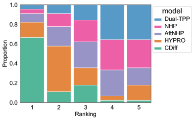
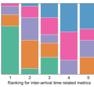
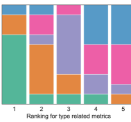
Figure 3: Left) Stacked column chart of ranks of the algorithms across the 5 datasets for all the metrics. We collect the rank for each metric ($9$ metrics in total, as we include additional metrics from the interval forecasting experiment described in the Appendix 9.1). The x-axis is the rank, and the y-axis is the proportion adding up to 1. Middle) Stacked column chart of ranks only for time-related metrics ($RMSE_{x}$, $MAPE$, $sMAPE$, $RMSE_{|\mathbf{s}|}$, $MAE_{|\mathbf{s}|}$). Right) Stacked column chart of ranks only for type-related metric ($RMSE_{e}$).

Table 1 presents results of a subset of our experiments for four selected metrics on real-world datasets. Complete results are in the Appendix 9.11. We test for significance using a paired Wilcoxon signed-rank test at the $5\%$ significance level.

Surprisingly, despite the explicit focus of Dual-TPP on multi-event forecasting, it is the weakest competing baseline. Although it targets longer horizons, it relies on an older TPP model that is significantly outperformed by more recent algorithms, including AttNHP and NHP.

In alignment with previous findings, AttNHP consistenly outperforms NHP, reaffirming AttNHP’s position as the SOTA method for single event forecasting. As expected, HYPRO ranks as the second-best competing baseline since it leverages AttNHP as its base model and is designed for multi-event forecasting. Our proposed method, CDiff, consistently outperforms the baselines. For most cases when CDiff ranks first, the performance difference is statistically significant. These trends remain consistent across all our experiments, datasets, and metrics, as illustrated in the summarizing ranking in Figure 3.

Figure 3(left) shows that CDiff is usually the top-ranked method and consistently outperforms the competing baselines. The middle and right panels of Figure 3 confirm that this ranking is maintained for both event type metrics and time interval metrics. This is not the case for all baselines; the single event forecasting baselines AttNHP and NHP both appear to face greater difficulties in predicting event types.

6.1 CDiff can model complex inter-arrivals

We first examine the learned marginal distribution for time intervals. We use the Taobao dataset for our analysis because it is a relatively challenging dataset, with 17 event types and a marginal distribution inter-arrival times that appears to be multi-modal. From the histograms of inter-arrival time prediction in Figure 4, we see that our CDiff model is better at capturing the ground truth distribution. CDiff is effective at generating both longer intervals, falling within the range of $(3h25-\infty]$, and shorter intervals, within the range of $(0-0.01h]$.

Figure 4: Histogram of true and predicted inter-arrival times for the Taobao dataset. Note that the bin widths gradually increase to make visual comparison easier.

In contrast, HYPRO and AttNHP, the most competitive models, struggle to generate a sufficient number of values at the extremities of the marginal distribution. This also impacts the methods’ ability to capture the joint relationship between time intervals and event types. To illustrate this, we consider two of the event categories $\mathcal{C}$ for Taobao dataset, and we plot the count histograms of the time intervals with category 7 and 16 in Figure 5.

First, it is noticeable that HYPRO and AttNHP fail to generate an adequate number of events for these specific categories, resulting in counts lower than the ground truth. In contrast, CDiff generates the appropriate quantity. This implies that CDiff is better at capturing the marginal categorical distribution of events. For both event types, the ground truth exhibits many very short intervals (the first bin) and then a rapid drop. CDiff manages to follow this pattern, while also accurately capturing the number of events in the tail (the final bin). HYPRO and AttNHP struggle to match the rapid decay. In the bottom panel, they also fail to produce many large inter-arrival times. These observations may be attributed to the fact that HYPRO and AttNHP rely on exponential distributions to model time intervals and are autoregressive whereas our architecture does not rely on a parametric TPP model and jointly models the distribution of the $N$ events in the sequence.

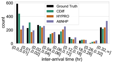
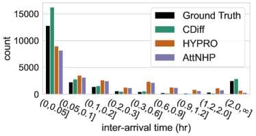
Figure 5: Histogram of true and predicted inter-arrival times for cases when the next event is type $e{=}7$ (top) and $e{=}16$ (bottom) for the Taobao dataset. Bin widths gradually increase so that counts are more comparable.

6.2 CDiff can forecast long horizon events

CDiff is explicitly designed to perform multi-event prediction, so we expect it to be better at predicting long horizon events, i.e., those near the end of the prediction horizon, such as events $N{-}1$ and $N$. To verify this, we examine the error $\delta_{i}$ for the i-th time-interval and the cumulated errors $c_{j}=\sum^{j}_{k=1}\mathbb{I}[\hat{e}_{k}=e_{k}]$ for the type. Hence, given a sequence to predict, we also have a sequence of time and type prediction errors: $[\delta_{1},\dots,\delta_{N}]$, $[c_{1},\dots,c_{N}]$ from which we can estimate the rate of increase/decrease of error using linear regression on each sequence. We denote these rates (slopes) by $s^{\delta}$ for interarrival time and $s^{c}$ for type. We then test whether one baseline consistently has a lower slope than another using a paired Wilcoxon signed-rank test at the $5\%$ significance level. Table 2 reports the results for time error and Table 3 for type error.

The error slopes are positive for all methods, as we would expect since the prediction task becomes increasingly difficult. Overall, CDiff has the lowest error slopes, with statistical significance in almost all instances. This means that CDiff’s error increases more slowly than the baselines, verifying our hypothesis that it is better at forecasting long horizon events. The next best method is HYPRO, which also targets multi-event forecasting. HYPRO even has the lowest slope in one instance (event type for Taxi), although without statistical significance w.r.t. CDiff.

Table 2: Average time error slope $s^{\delta}$ for different dataset. * indicates stat. significance w.r.t to the best method.

baseline	Synthetic	Taxi	Taobao	Stackoverflow
HYPRO	$0.465^{*}$	0.182	$1.501^{*}$	1.244
Attnhp	$0.423^{*}$	$0.218^{*}$	$1.416^{*}$	$1.567^{*}$
NHP	$0.549^{*}$	$0.195^{*}$	$2.825^{*}$	$2.058^{*}$
DualTPP	$0.519^{*}$	$0.202^{*}$	$2.593^{*}$	$1.518^{*}$
CDiff	0.226	0.171	1.372	1.238

Table 3: Average type error slope $s^{c}$ for different dataset. * indicates stat. significance w.r.t to the best method.

baseline	Synthetic	Taxi	Taobao	Stackoverflow
HYPRO	$0.851$	0.436	$0.724^{*}$	$0.795^{*}$
Attnhp	$0.858^{*}$	$0.508^{*}$	$0.758^{*}$	$0.800^{*}$
NHP	$0.857^{*}$	$0.538^{*}$	$0.842^{*}$	$0.799^{*}$
DualTPP	$0.850^{*}$	$0.502^{*}$	$0.793^{*}$	$0.795^{*}$
CDiff	0.839	0.439	0.719	0.775

6.3 Forecasting shorter horizons

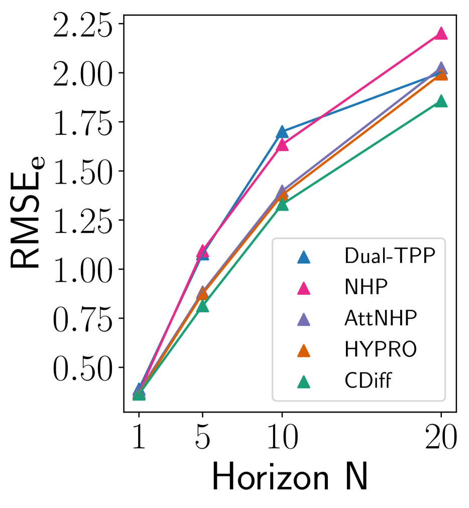
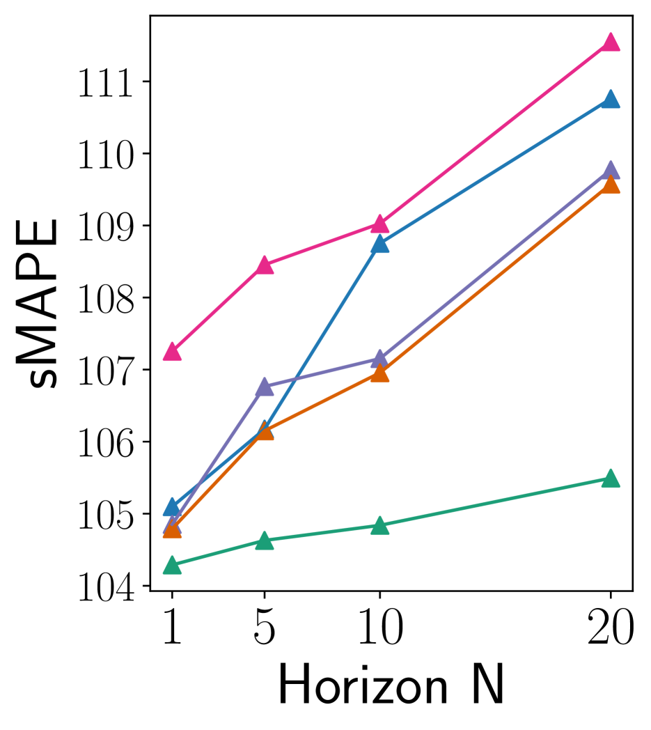
Figure 6: $RMSE_{e}$ and $sMAPE$, averaged over all datasets, for different horizons.

Table 4: Complexity analysis on three datasets for $N=20$. The training time is for 500 epochs. The experiments were run on a GeForce RTX 2070 SUPER machine.

		HYPRO	DualTPP	Attnhp	NHP	CDiff
Taxi	Sampling (sec/$\mathbf{s}_{u}$ )	0.265	0.158	0.136	0.145	0.104
	num. param. (K)	40.5	40.1	19.3	19.3	17.1
	Training (mins)	95	45	35	35	35
Taobao	Sampling (sec/$\mathbf{s}_{u}$ )	0.325	0.240	0.209	0.227	0.129
	num. param. (K)	40.1	19.7	19.6	40.0	62.6
	Training (mins)	105	60	45	45	45
Stack.	Sampling (sec/$\mathbf{s}_{u}$ )	0.294	0.207	0.191	0.200	0.133
	num. param. (K)	41.0	40.3	20.1	20.0	63.9
	Training (mins)	105	60	45	45	45

Figure 6 presents the results for shorter horizons: $N=1,5,10$. All methods improve as we reduce the forecasting horizon. For $RMSE_{\mathbf{e}}$, all models perform similarly to $N=20$. The performance difference grows as the prediction horizon increases. For $sMAPE$, CDiff outperforms the other models even for single event forecasting, and the outperformance increases rapidly with the prediction horizon. We attribute this to CDiff’s ability to model more complex inter-arrival distributions.

6.4 Sampling and Training efficiency

Table 4 summarizes the sampling time, number of trainable parameters, and training time for all methods across three datasets. Starting with sampling time, we observe that CDiff is significantly faster. This is expected because the baselines are autoregressive, whereas CDiff generates the entire sequence at once. We do employ optimized diffusion sampling. Dual-TPP, NHP, and AttNHP are all RNN-based, leading to similar sampling times. HYPRO is the slowest because it generates multiple proposed sequences that are filtered by a selection module.

Regarding space complexity, CDiff generally has the largest number of parameters (except for Taxi, which is a simpler task) as the dimension of the predicted vectors is $N$ times larger than all the other methods that generate one event at a time. HYPRO and Dual-TPP are both larger than NHP and AttNHP as they have additional components dedicated to long horizon forecasting. Finally, turning to training time, CDiff, NHP, and AttNHP are the fastest. Dual-TPP is slower to train due to its joint count component. HYPRO requires much more training time because it has to generate samples as part of its training process to train the selection modules.

7 LIMITATIONS

Although offering impressive performance, there are limitations specific to our approach of modelling $N$ events at once. Unlike previous autoregressive approaches, our method requires the practitioner to select a fixed number of events $N$ to be modeled by the diffusion generative model. This can prove challenging when dealing with data that exhibits highly irregular time intervals ($x_{i}$). Essentially, if the length of time spanned by a fixed number of events varies significantly, then it will lead to a substantial variation in the nature and complexity of the forecasting task. This effect was not observed in the datasets we considered, as none displayed such high irregularities.

8 CONCLUSION

We have proposed a diffusion-based generative model, CDiff, for event sequence forecasting. Extensive experiments demonstrate the superiority of our approach over existing baselines for long horizons. The approach also offers improved sampling efficiency. Our analysis sheds light on the mechanics behind the improvements, revealing that our model excels at capturing intricate correlation structure and at predicting distant events.

9 Appendix

9.1 Interval Forecasting

In this time-based setting, the task is to predict the events that occur within a given subsequent time interval $t^{\prime}$, i.e., $\mathbf{s}_{u}$: $\mathbf{x}_{u}=[x_{I+1},...]$ and $\mathbf{e}_{u}=[e_{I+1},...]$ such that $||\mathbf{x}_{u}||_{1}\leq t^{\prime}$.

This different setting also calls for different metrics, and the predicted $\hat{\mathbf{s}}_{u}$ and ground truth $\mathbf{s}_{u}$ can have a different number of events. We report both $OTD$ and the $RMSE_{e}$ metrics as they are robust to a varying number of events. We also report additional metrics that compare the number of events predicted:

1. $MAE_{|\mathbf{s}|}={\frac{1}{M}\sum_{j=1}^{M}\big{|}|\mathbf{s}_{u}^{j}|-|\hat{\mathbf{s}}_{u}^{j}|\big{|}}$;

2. $RMSE_{|\mathbf{s}|}=\sqrt{\frac{1}{M}\sum_{j=1}^{M}(|\mathbf{s}_{u}^{j}|-|\hat{\mathbf{s}}_{u}^{j}|)^{2}}$.

For our experiment, we retain the same context sequences $\mathbf{s}_{c}$ that were used for the next $N$ events forecasting setting.. Table 5 details the time interval values $t^{\prime}$ of three experiments (long, medium and short horizon) for each dataset.

Table 5: Time interval for interval forecasting problem.

Dataset	$t^{\prime}$ long	$t^{\prime}$ medium	$t^{\prime}$ short	train/val/test	units
Synthetic	2	1	0.5	1500/400/500	second
Taxi	4.5	2.25	1.125	1300/200/400	hour
Taobao	19.5	9.25	5.25	1300/200/500	hour
Stack.	220	110	55	1400/400/400	day
Retweet	500	250	150	1400/600/800	second

9.2 CDiff methodology for interval Forecasting

To adapt our CDiff model to this setting, we select a number of events, denoted as $N$, and repeatedly generate $N$-length sequences until we reach the end of the forecasting window $t^{\prime}$. That is, while $||\mathbf{x}_{u}||_{1}\leq t^{\prime}$, we integrate the current $\mathbf{s}_{u}$ into the context $\mathbf{s}_{c}$ and regenerate $N$ additional events that we attach at the end of $\mathbf{s}_{u}$. We set $N$ to be the maximum number of events observed within the given time interval in the training data.

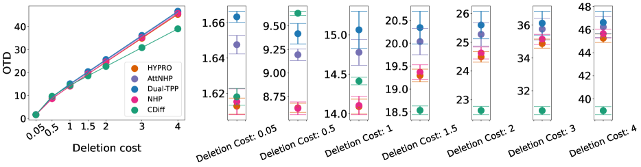
(a) Synthetic dataset for $N=20$ forecasting

(b) Taxi dataset without for $N=20$ forecasting

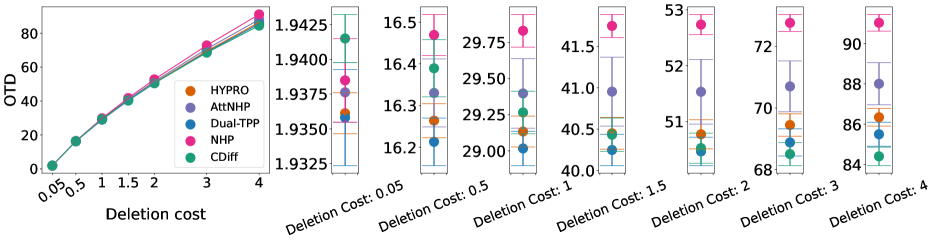
(c) Stackoverflow dataset for $N=20$ forecasting

(d) Taobao dataset $N=20$ forecasting

(e) Retweet dataset $N=20$ forecasting

Figure 7: OTD for each specific deletion/addition cost for $N=20$ forecasting, we chose a variety of $C_{\text{del}}$ values—$0.05,0.5,1,1.5,2,3,4$—based on the recommendations in (Xue et al.,, 2022). Subsequently, we calculated the mean and s.d. of OTD across all the datasets.

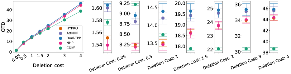
(a) Synthetic dataset interval forecasting

(b) Taxi dataset interval forecasting

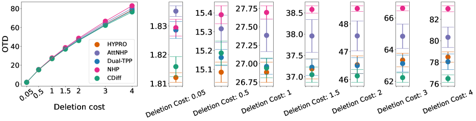
(c) Stackoverflow dataset interval forecasting

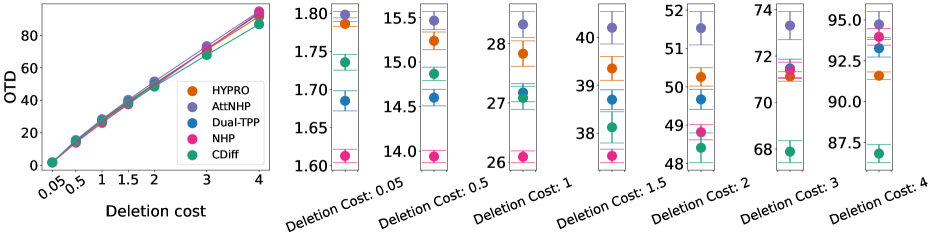
(d) Taobao dataset interval forecasting

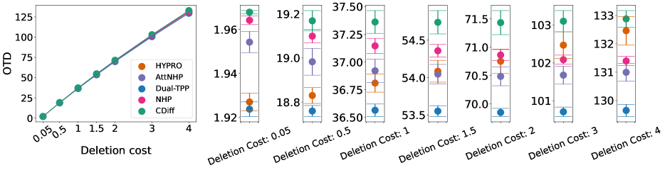
(e) Retweet dataset interval forecasting

Figure 8: OTD for each specific deletion/addition cost for interval forecasting. We calculated the mean and s.d. of OTD across all the datasets for different $C_{\text{del}}$ values.

9.3 OTD metric and more OTD results

In the calculation of Optimal Transport Distance (OTD), the deletion cost hyperparameter, denoted by $C_{\text{del}}$, plays a pivotal role. Yang et al., (2022) provided a full description and pseudo code for the dynamic algirthm to calculate the OTD. This parameter quantifies the expense associated with the removal or addition of an event token, irrespective of its category. For our experimentation, we chose a variety of $C_{\text{del}}$ values—$0.05,0.5,1,1.5,2,3,4$—based on the recommendations provided by Xue et al., (2022). Subsequently, we calculated the mean OTD. In the following section, the OTD metrics are delineated for each individual $C_{\text{del}}$ value. As evidenced by Fig. 7 and 8, our model outperforms across the board for the varying $C_{\text{del}}$ settings overall. We also see that the OTD steadily increases overall, and that different C can permute the ordering of the competing baselines. For low $C_{\text{del}}$, our method is outperformed by HYPRO and AttNHP sometimes, but this trend is reversed for larger $C_{\text{del}}$ values for almost all datasets. This reflects the fact that the proposed CDiff method is better at predicting the number of events, so fewer deletions or additions are required.

9.4 Dataset details

• Taobao (Alibaba,, 2018) This dataset captures user click events on Taobao’s shopping websites between November 25 and December 03, 2017. Each user’s interactions are recorded as a sequence of item clicks, detailing both the timestamp and the item’s category. All item categories were ranked by frequency, with only the top 16 retained; the remaining were grouped into a single category. Thus, we have $K=17$ distinct event types, each corresponding to a category. The refined dataset features 2,000 of the most engaged users, with an average sequence length of 58. The disjoint train, validation and test sets consist of 1300, 200, and 500 sequences (users), respectively, randomly sampled from the dataset. The time unit is $3$ hours; the average inter-arrival time is $0.06$ (i.e., $0.18$ hour).

• Taxi (Whong,, 2014) This dataset contains time-stamped taxi pickup and drop off events with zone location ids in New York city in 2013. Following the processing procedure of Mei et al., (2019), each event type is defined as a tuple of (location, action). The location is one of the $5$ boroughs (Manhattan, Brooklyn, Queens, The Bronx, Staten Island). The action can be either pick-up or drop-off. Thus, there are $K=5\times 2=10$ event types in total. The values $k=0,\ldots,4$ indicate pick-up events and $k=5,\ldots,9$ indicate drop-off events. A subset of 2000 sequences of taxi pickup events with average length 39 are retained. The average inter-arrival time is $0.22$ hour (time unit is $1$ hour.) The disjoint train, validation and test sets are randomly sampled and are of sise 1400, 200, and 400 sequences, respectively.

• StackOverflow (Leskovec and Krevl,, 2014) This dataset contains two years of user awards from a question-answer platform. Each user was awarded a sequence of badges, with a total of $K=22$ unique badge types. The train, validation and test sets consist of $1400$, $400$ and $400$ sequences, resepctively, and are randomly sampled from the dataset. The time unit is $11$ days; the average inter-arrival time is $0.95$.

• Retweet (Zhou et al.,, 2013) This dataset contains sequences of user retweet events, each annotated with a timestamp. These events are segregated into three categories ($K=3$), denoted by: “small”, “medium”, and “large” users. Those with under 120 followers are labeled as small users; those with under 1363 followers are medium users, while the remaining users are designated as large users. Our studies focus on a subset of 9000 retweet event sequences. The disjoint train, validation and test sets consist of 6000, 1500, and 1500 sequences, respectively, randomly sampled from the dataset.

• Synthetic Multivariate Hawkes Dataset The synthetic dataset is generated using the tick package provided by Bacry et al., (2018), using the Hawkes process generator. Our study uses the same equations proposed by Lin et al., (2022). There are 5 event types. The impact function $g_{j,i}(y)$ measuring the relationship (impact) of type $i$ on type $j$ and is uniformly-randomly chosen from the following four functions:

  $$\begin{split}g_{a}(y)&=0.99\exp(-0.4y)\\ g_{b}(y)&=0.01\exp(-0.8y)+0.03\exp(-0.6y)+0.05\exp(-0.4y)\\ g_{c}(y)&=0.25|\cos 3y|\exp(-0.1y)\\ g_{d}(y)&=0.1(0.5+y)^{2}\end{split}$$ (31)

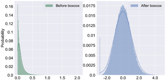
Figure 9: Inter-arrival time marginal histogram for synthetic dataset before (left) and after (right) boxcox transformation

9.5 Box-cox Transformation

For our study, the inter-arrival time marginal distribution shown in Fig.9 (left) is clearly not a normal distribution. Since the diffusion probabilistic model we employ is a Gaussian-based generative model, we use the Box-Cox transformation to transform the inter-arrival time data, so that the transformed data approximately obeys a normal distribution.

The Box-Cox transformation (Tukey,, 1957) is a family of power transformations that are used to stabilize variance and make data more closely follow a normal distribution. The transformation is defined as:

$$x(\lambda)=\begin{cases}\frac{x^{\lambda}-1}{\lambda}&\text{if }\lambda\neq 0,\\ \log(x)&\text{if }\lambda=0.\end{cases}$$ (32)

Here:

• $x$ is the original data;

• $x(\lambda)$ is the transformed data; and

• $\lambda$ is the transformation parameter.

The inter-arrival time is strictly larger than 0 but it can be extremely small because of the scale of the dataset. Therefore, in order to prevent numerical errors in tbe Box-Cox transformation we add $1\times 10^{-7}$ time units to all inter-arrival times. We then scale all values by $100$. We use the scaled inter-arrival time data from the train set to obtain the fitted $\lambda$ shown in Eq.32 and apply the transformation with the fitted $\lambda$ to the inter-arrival time data for both the validation dataset and test dataset. Fig.9 shows an example of marginal histogram of inter-arrival time for the Synthetic train set before (left) and after (right) the Box-cox transformation. We transform back the predicted sequence inter-arrival times with the same fitted $\lambda$ obtained from the train set and undo the scaling by 100. We use the Box-cox transformation function from the SciPy package provided by Virtanen et al., (2020).

Table 6: Sets of hyperparameters. Underlined values are those selected by the Tree-Structured Parzen Estimator (Bergstra et al.,, 2011)

Parameters	num. heads	num. layers	time embedding	Transformer feed-forward embedding	num. diffusion steps	LR
Synthetic	{1,$\underline{2}$,4}	{1, 2, 4}	{4, 8, 16, 32, 64, 128}	{8, 16, 32, 64, 128, 256}	{50, 100, 200, 300, 500}	{0.001, 0.0025, 0.005}
Taxi	{1,$\underline{2}$,4}	{1, 2, 4}	{4, 8, 16, 32, 64, 128}	{8, 16, 32, 64, 128, 256}	{50, 100, 200, 300, 500}	{0.001, 0.0025, 0.005}
Taobao	{1,$\underline{2}$,4}	{1, 2, 4}	{4, 8, 16, 32, 64, 128}	{8, 16, 32, 64, 128, 256}	{50, 100, 200, 300, 500}	{0.001, 0.0025, 0.005}
Stackoverflow	{1,$\underline{2}$,4}	{1, 2, 4}	{4, 8, 16, 32, 64, 128}	{8, 16, 32, 64, 128, 256}	{50, 100, 200, 300, 500}	{ 0.001, 0.0025, 0.005}
Retweet	{1,$\underline{2}$,4}	{1, 2, 4}	{4, 8, 16, 32, 64, 128}	{8, 16, 32, 64, 128, 256}	{50, 100, 200, 300, 500}	{0.001, 0.0025, 0.005}

9.6 Hyper-parameters

Table 6 specifies the hyperparameters that we use for our experiments and the candidate values. We train for a maximum of 500 epochs and we select the best hyperparameters using the Tree-Structured Parzen Estimator (Bergstra et al.,, 2011).

9.7 Sampling Details

In order to achieve a faster sampling time, we leverage the work of Song et al., (2021). We can re-express Eq.11 as follows

$$\mathbf{x}_{t-1} =\sqrt{\bar{\alpha}_{t-1}}(\frac{\mathbf{x}_{t}-\sqrt{1-\bar{\alpha}_{t}}\epsilon_{\theta}(\mathbf{x}_{t},t,\mathbf{e}_{t},\mathbf{s}_{c})}{\sqrt{\bar{\alpha}_{t}}})+\sqrt{1-\bar{\alpha}_{t-1}-\sigma_{t}^{2}}\cdot\epsilon_{\theta}(\mathbf{x}_{t},t,\mathbf{e}_{t},\mathbf{s}_{c})+\sigma_{t}\mathbf{z}$$ (33)

Given a trained DDPM model, we can specify $\{\sigma_{t}\}^{\tau}_{t=1}$ and specify $\tau\subset\{1,2,..,T\}$ to accomplish the acceleration. In Eq.33, if we set $\sigma_{t}=0$ then we are performing DDIM (Denoising Diffusion Implicit Model) acceleration as in (Song et al.,, 2021). For event type acceleration, we choose to directly jump steps, because for multinomial diffusion (Hoogeboom et al.,, 2021), instead of predicting noise, we predict $\mathbf{e}_{0}$. Therefore, our acceleration relies on decreasing the number of times we recalculate $\hat{\mathbf{e}}_{0}=\phi_{\theta}(\mathbf{e}_{t},\mathbf{x}_{t},t,\mathbf{s}_{c})$. That is, given a sub-set $\tau\subset\{1,2,..,T\}$, we only recalculate $\hat{\mathbf{e}}_{0}$ $|\tau|$ times. In practice, we found it does not harm the prediction but it significantly accelerates the sampling due to $\phi_{\theta}(\cdot)$ requiring the majority of the computation effort.

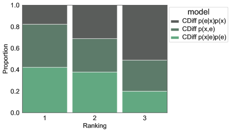
Figure 10: 100% Stacked column chart of ranks of different CDiff across the 5 datasets for all the metrics.

9.8 Comparison with $p(\mathbf{x},\mathbf{e})$ and $p(\mathbf{e}|\mathbf{x})p(\mathbf{x})$

Mathematically, $p(\mathbf{x},\mathbf{e})=p(\mathbf{e}|\mathbf{x})p(\mathbf{e})=p(\mathbf{x}|\mathbf{e})p(\mathbf{e})$, so there should not be any theoretical difference between sampling the event type and interarrival time jointly or sampling one first and then the other, conditioned on the first. We conducted an experiment to check that this was also observed in the practical implementation. Fig.10 shows that the order of sampling does not have a major effect, although there is a minor advantage to either jointly sampling from $p(\mathbf{x},\mathbf{e})$ or sampling the event type first (i.e., from $p(\mathbf{e}|\mathbf{x})p(\mathbf{e})$). This perhaps reflects that it is easier to learn the conditional inter-arrival time distributions, which may have slightly simpler structure.

9.9 Positional Encoding for CDiff

We use the transformer architecture as a denoising tool for reversing the diffusion processes. Therefore, we encode the position of both the diffusion step and the event token’s order.

It is important that our choice of encoding can differentiate between these two different types of position information. To achieve this, we use as input $(i+y_{N})$, where $i$ is the order of the event token in the noisy event sequence, and $y_{N}$ is the last timestamp of the historical event sequence.

into Eq. 30 (shown also below) for the order of the predicted sequence. This approach distinctly differentiates the positional information of the predicted event sequence from the diffusion time step’s positional encoding. The positional encoding is then:

$$[\mathbf{m}(y_{j},D)]_{i}=\left\{\begin{aligned} \cos(y_{j}/10000^{\frac{i-1}{D}})\quad\text{if $i$ is odd\,,}\\ \sin(y_{j}/10000^{\frac{i}{D}})\quad\text{if $i$ is even.}\end{aligned}\right.$$ (34)

9.10 More Diffusion Visualization

Figure 11 shows the reverse process of CDiff for Taxi dataset (on the left) and Taobao dataset (on the right). Upon inspection, it is evident that the recovered sequences bear a strong resemblance to their respective ground truth sequences, both in terms of inter-arrival time patterns and event classifications.

In the Taxi dataset, the original sequences prominently feature events colored in Cyan and Orange. This indicates a high frequency of these two event categories, a pattern which is consistently replicated in the sequences derived from CDiff.

Conversely, for the Taobao dataset, the ground truth predominantly showcases shorter inter-arrival times, signifying closely clustered events. However, there are also occasional extended inter-arrival times introducing gaps in the sequences. Notably, this dichotomy is accurately reflected in the reconstructed sequences.

Figure 11: Visualization of the cross-diffusion generating process for 15 examples sequences of the Taxi dataset (left) and the Taobao dataset (right). The colors indicates the different categories. We start by generating noisy sequences ($t=T$). Once we reach the end of the denoising process ($t=0$), we have recovered sequences similar to the ground truth sequences. We cut the sequence based on the time range so that every sequence can be aligned.

9.11 Tables of results with different evaluation metrics for different horizon

Tables 7, 8 and 9 show the results of all metrics across all models for all datasets with different prediction horizons. We test for significance using a paired Wilcoxon signed-rank test at the 5% significance level.

Table 7: Results for all metrics across 5 different datasets for $N=20$ events forecasting and long interval forecasting, bold case indicates the best, under line indicates the second best, * indicates stats. significance w.r.t. the method with the lowest value.

	Synthetic dataset
	$N=20$ events forecasting					Interval forecasting $t^{\prime}$ long
	OTD	$\textbf{RMSE}_{e}$	$\textbf{RMSE}_{x}$	MAPE	sMAPE	OTD	$\textbf{RMSE}_{e}$	$\textbf{RMSE}_{|\mathbf{s}|}$	$\textbf{MAE}_{|\mathbf{s}|}$
HYPRO	20.609 $\pm$ 0.328	2.464 $\pm$ 0.039	$\text{\text@underline{0.104 $\pm$ 0.002}}^{*}$	717.417 $\pm$ 56.443	$\text{100.535 $\pm$ 0.084}^{*}$	$\text{\text@underline{ 20.224 $\pm$ 0.236}}^{*}$	2.409 $\pm$ 0.082	1.608 $\pm$ 0.103	0.573 $\pm$ 0.049
Dual-TPP	$\text{22.117 $\pm$ 0.368}^{*}$	$\text{2.506 $\pm$ 0.044}^{*}$	$\text{0.108 $\pm$ 0.001}^{*}$	$\text{724.681 $\pm$ 28.097}^{*}$	$\text{100.857 $\pm$ 0.624}^{*}$	$\text{21.521 $\pm$ 0.375}^{*}$	$\text{2.511 $\pm$ 0.050}^{*}$	$\text{2.297 $\pm$ 0.117}^{*}$	$\text{0.952 $\pm$ 0.057}^{*}$
Attnhp	$\text{21.843 $\pm$ 0.316}^{*}$	$\text{2.509 $\pm$ 0.051}^{*}$	$\text{0.104 $\pm$ 0.004}^{*}$	682.086 $\pm$ 63.199	$\text{101.117 $\pm$ 0.295}^{*}$	$\text{21.153 $\pm$ 0.206}^{*}$	$\text{2.509 $\pm$ 0.048}^{*}$	$\text{2.806 $\pm$ 0.073}^{*}$	$\text{0.809 $\pm$ 0.033}^{*}$
NHP	$\text{21.541 $\pm$ 0.203}^{*}$	$\text{\text@underline{2.462 $\pm$ 0.018}}^{*}$	$\text{0.109 $\pm$ 0.001}^{*}$	$\text{786.866 $\pm$ 31.782}^{*}$	$\text{\text@underline{99.622 $\pm$ 0.426}}^{*}$	$\text{20.541 $\pm$ 0.203}^{*}$	$\text{2.462 $\pm$ 0.021}^{*}$	1.411 $\pm$ 0.048	$\text{\text@underline{0.588 $\pm$ 0.013}}^{*}$
CDiff	19.788 $\pm$ 0.343	2.375 $\pm$ 0.021	0.098 $\pm$ 0.02	668.287 $\pm$ 51.873	98.933 $\pm$ 0.573	19.674 $\pm$ 0.125	2.370 $\pm$ 0.061	1.932 $\pm$ 0.094	$\text{0.812 $\pm$ 0.051}^{*}$
	Taxi dataset
	$N=20$ events forecasting					Interval forecasting $t^{\prime}$ long
	OTD	$\textbf{RMSE}_{e}$	$\textbf{RMSE}_{x}$	MAPE	sMAPE	OTD	$\textbf{RMSE}_{e}$	$\textbf{RMSE}_{|\mathbf{s}|}$	$\textbf{MAE}_{|\mathbf{s}|}$
HYPRO	21.653 $\pm$ 0.163	$\text{\text@underline{1.231 $\pm$ 0.015}}^{*}$	$\text{\text@underline{0.372 $\pm$ 0.004}}^{*}$	252.761 $\pm$ 6.827	$\text{\text@underline{93.803 $\pm$ 0.454}}^{*}$	19.632 $\pm$ 0.179	1.550 $\pm$ 0.026	$\text{\text@underline{4.326 $\pm$ 0.063}}^{*}$	$\text{\text@underline{2.781 $\pm$ 0.088}}^{*}$
Dual-TPP	${24.483\pm 0.383}^{*}$	$\text{1.353 $\pm$ 0.037}^{*}$	$\text{0.402 $\pm$ 0.006}^{*}$	$\text{285.590 $\pm$ 8.088}^{*}$	$\text{95.211 $\pm$ 0.187}^{*}$	$\text{20.952 $\pm$ 0.278}^{*}$	$\text{1.627 $\pm$ 0.033}^{*}$	$\text{4.995 $\pm$ 0.150}^{*}$	$\text{3.795 $\pm$ 0.107}^{*}$
Attnhp	${24.762\pm 0.217}^{*}$	$\text{1.276 $\pm$ 0.015}^{*}$	${0.430\pm 0.003}^{*}$	$\text{286.869 $\pm$ 9.973}^{*}$	$\text{97.388 $\pm$ 0.381}^{*}$	$\text{20.588 $\pm$ 0.208}^{*}$	1.590 $\pm$ 0.024	$\text{4.915 $\pm$ 0.116}^{*}$	$\text{3.509 $\pm$ 0.112}^{*}$
NHP	$\text{25.114 $\pm$ 0.268}^{*}$	${1.297\pm 0.019}^{*}$	${0.399\pm 0.040}^{*}$	$\text{281.306 $\pm$ 8.271}^{*}$	$\text{96.459 $\pm$ 0.521}^{*}$	$\text{21.134 $\pm$ 0.148}^{*}$	$\text{1.632 $\pm$ 0.030}^{*}$	$\text{4.883 $\pm$ 0.119}^{*}$	$\text{3.526 $\pm$ 0.135}^{*}$
CDiff	21.013 $\pm$ 0.158	1.131 $\pm$ 0.017	0.351 $\pm$ 0.004	243.2 $\pm$ 7.725	87.993 $\pm$ 0.178	19.028 $\pm$ 0.224	1.329 $\pm$ 0.029	3.690 $\pm$ 0.097	2.593 $\pm$ 0.124
	Taobao dataset
	$N=20$ events forecasting					Interval forecasting $t^{\prime}$ long
	OTD	$\textbf{RMSE}_{e}$	$\textbf{RMSE}_{x}$	MAPE	sMAPE	OTD	$\textbf{RMSE}_{e}$	$\textbf{RMSE}_{|\mathbf{s}|}$	$\textbf{MAE}_{|\mathbf{s}|}$
HYPRO	44.336 $\pm$0.127	$\text{\text@underline{2.710 $\pm$0.021}}^{*}$	$\text{\text@underline{0.594 $\pm$0.030}}^{*}$	6397.66 $\pm$ 154.977	$\text{134.922 $\pm$ 0.473}^{*}$	$\text{42.525 $\pm$ 0.151 }^{*}$	2.810 $\pm$ 0.028	4.022 $\pm$ 0.067	$\text{3.019 $\pm$ 0.017}^{*}$
Dual-TPP	$\text{47.324 $\pm$ 0.541}^{*}$	$\text{3.237 $\pm$ 0.049}^{*}$	$\text{0.871 $\pm$0.014}^{*}$	$\text{8325.564 $\pm$ 245.765}^{*}$	$\text{141.687 $\pm$ 0.431}^{*}$	$\text{\text@underline{38.530 $\pm$ 0.263}}^{*}$	$\text{4.439 $\pm$ 0.019}^{*}$	$\text{5.893 $\pm$ 0.088}^{*}$	$\text{3.832 $\pm$ 0.016}^{*}$
Attnhp	$\text{45.555 $\pm$ 0.345}^{*}$	2.737 $\pm$ 0.021	$\text{0.708 $\pm$ 0.011}^{*}$	6250.83 $\pm$ 265.440	$\text{\text@underline{134.582 $\pm$ 0.920}}^{*}$	$\text{43.624 $\pm$ 0.282}^{*}$	2.855 $\pm$ 0.020	4.097 $\pm$ 0.016	2.892 $\pm$ 0.024
NHP	$\text{48.131 $\pm$ 0.297}^{*}$	$\text{3.355 $\pm$ 0.030}^{*}$	$\text{0.837 $\pm$ 0.009}^{*}$	$\text{7909.437 $\pm$ 149.274}^{*}$	$\text{137.644 $\pm$ 0.764}^{*}$	38.204 $\pm$ 0.302	$\text{3.515 $\pm$ 0.028}^{*}$	$\text{5.41 $\pm$ 0.081}^{*}$	$\text{3.998 $\pm$ 0.027}^{*}$
CDiff	44.621 $\pm$ 0.139	2.653 $\pm$ 0.011	0.551 $\pm$ 0.013	6850.359 $\pm$ 165.400	125.685 $\pm$ 0.151	$\text{40.783 $\pm$ 0.059}^{*}$	2.831 $\pm$ 0.009	4.103 $\pm$ 0.034	2.947 $\pm$0.019
	Stackoverflow dataset
	$N=20$ events forecasting					Interval forecasting $t^{\prime}$ long
	OTD	$\textbf{RMSE}_{e}$	$\textbf{RMSE}_{x}$	MAPE	sMAPE	OTD	$\textbf{RMSE}_{e}$	$\textbf{RMSE}_{|\mathbf{s}|}$	$\textbf{MAE}_{|\mathbf{s}|}$
HYPRO	42.359 $\pm$ 0.170	1.140 $\pm$ 0.014	$\text{1.554 $\pm$ 0.010}^{*}$	$\text{2013.055 $\pm$ 160.862}^{*}$	$\text{110.988 $\pm$ 0.559}^{*}$	38.460 $\pm$ 0.204	1.294 $\pm$ 0.016	$\text{\text@underline{2.672 $\pm$ 0.019}}^{*}$	1.496 $\pm$ 0.017
Dual-TPP	41.752 $\pm$ 0.200	1.134 $\pm$ 0.019	$\text{1.514 $\pm$ 0.017}^{*}$	$\text{1729.83 $\pm$ 67.928}^{*}$	$\text{117.582 $\pm$ 0.420}^{*}$	38.474 $\pm$ 0.274	1.364 $\pm$ 0.019	$\text{3.332 $\pm$ 0.088}^{*}$	$\text{1.753 $\pm$ 0.036}^{*}$
Attnhp	$\text{42.591 $\pm$ 0.408}^{*}$	1.145 $\pm$ 0.011	1.340 $\pm$ 0.006	1519.740 $\pm$ 52.216	108.542 $\pm$0.531	$\text{39.76 $\pm$ 0.373}^{*}$	$\text{1.385 $\pm$ 0.014}^{*}$	$\text{3.424 $\pm$ 0.023}^{*}$	$\text{1.813 $\pm$ 0.014}^{*}$
NHP	$\text{43.791 $\pm$ 0.147}^{*}$	$\text{1.244 $\pm$ 0.030}^{*}$	$\text{1.487 $\pm$ 0.004}^{*}$	$\text{1693.977 $\pm$ 113.300}^{*}$	$\text{116.952 $\pm$ 0.404}^{*}$	$\text{40.453 $\pm$ 0.188}^{*}$	$\text{1.447 $\pm$ 0.012}^{*}$	$\text{3.552 $\pm$ 0.051}^{*}$	$\text{1.793 $\pm$ 0.057}^{*}$
CDiff	41.245 $\pm$ 1.400	1.141 $\pm$ 0.007	1.199 $\pm$ 0.006	1667.884 $\pm$ 32.220	106.175 $\pm$ 0.340	37.659 $\pm$ 0.334	$\text{1.421 $\pm$ 0.015}^{*}$	1.726 $\pm$ 0.043	1.239 $\pm$ 0.029
	Retweet dataset
	$N=20$ events forecasting					Interval forecasting $t^{\prime}$ long
	OTD	$\textbf{RMSE}_{e}$	$\textbf{RMSE}_{x}$	MAPE	sMAPE	OTD	$\textbf{RMSE}_{e}$	$\textbf{RMSE}_{|\mathbf{s}|}$	$\textbf{MAE}_{|\mathbf{s}|}$
HYPRO	$\text{61.031 $\pm$ 0.092}^{*}$	$\text{2.623 $\pm$ 0.036}^{*}$	$\text{30.100 $\pm$ 0.413}^{*}$	$\text{19686.811 $\pm$ 966.339}^{*}$	106.110 $\pm$ 1.505	59.292 $\pm$ 0.197	3.011 $\pm$ 0.029	3.109 $\pm$ 0.092	1.858 $\pm$ 0.067
Dual-TPP	$\text{61.095 $\pm$ 0.101}^{*}$	$\text{2.679 $\pm$ 0.026}^{*}$	28.914 $\pm$ 0.300	$\text{17619.400 $\pm$ 1003.001}^{*}$	106.900 $\pm$ 1.293	59.164 $\pm$ 0.069	$\text{2.981 $\pm$ 0.041}^{*}$	$\text{\text@underline{2.548 $\pm$ 0.133}}^{*}$	$\text{1.608 $\pm$ 0.028}^{*}$
Attnhp	60.634 $\pm$ 0.097	2.561 $\pm$ 0.054	$\text{28.812 $\pm$ 0.272}^{*}$	15396.198 $\pm$ 1058.618	$\text{107.234 $\pm$ 1.293}^{*}$	59.302 $\pm$ 0.160	2.832 $\pm$ 0.057	2.736 $\pm$ 0.119	1.554 $\pm$ 0.084
NHP	60.953 $\pm$ 0.079	$\text{2.651 $\pm$ 0.045}^{*}$	27.130 $\pm$ 0.224	15824.614 $\pm$ 1039.258	$\text{107.075 $\pm$ 1.398}^{*}$	59.395 $\pm$ 0.098	2.780 $\pm$ 0.046	$\text{2.649 $\pm$ 0.104}^{*}$	$\text{1.650 $\pm$ 0.044}^{*}$
CDiff	60.661 $\pm$ 0.101	2.293 $\pm$ 0.034	27.101 $\pm$ 0.113	16895.629 $\pm$ 741.331	106.184 $\pm$ 1.121	59.744 $\pm$ 0.574	2.661 $\pm$ 0.030	2.132 $\pm$ 0.131	1.088 $\pm$ 0.031

Table 8: Results for all metrics across 5 different datasets for $N=10$ events forecasting and medium interval forecasting, bold case indicates the best, under line indicates the second best, * indicates stats. significance w.r.t. the method with the lowest value

	Synthetic dataset
	$N=10$ events forecasting					Interval forecasting $t^{\prime}$ medium
	OTD	$\textbf{RMSE}_{e}$	$\textbf{RMSE}_{x}$	MAPE	sMAPE	OTD	$\textbf{RMSE}_{e}$	$\textbf{RMSE}_{|\mathbf{s}|}$	$\textbf{MAE}_{|\mathbf{s}|}$
HYPRO	12.962 $\pm$ 0.128	1.747 $\pm$ 0.041	0.104 $\pm$ 0.006	612.354 $\pm$ 21.017	99.473 $\pm$ 0.767	13.263 $\pm$ 0.213	1.721 $\pm$ 0.011	1.404 $\pm$ 0.023	0.561 $\pm$ 0.029
Dual-TPP	$\text{14.141 $\pm$ 0.125}^{*}$	$\text{1.965 $\pm$ 0.053}^{*}$	$\text{0.108 $\pm$ 0.008}^{*}$	$\text{713.157 $\pm$ 30.615}^{*}$	$\text{99.688 $\pm$ 0.672}^{*}$	$\text{13.919 $\pm$0.271}^{*}$	$\text{1.777 $\pm$ 0.019}^{*}$	$\text{2.109 $\pm$ 0.048}^{*}$	$\text{0.667 $\pm$ 0.033}^{*}$
Attnhp	13.916 $\pm$ 0.110	$\text{1.851 $\pm$ 0.039}^{*}$	0.103 $\pm$ 0.009	587.161 $\pm$ 41.113	$\text{100.041 $\pm$ 0.551}^{*}$	13.654 $\pm$ 0.163	$\text{1.799 $\pm$ 0.018}^{*}$	$\text{1.517 $\pm$ 0.045}^{*}$	$\text{0.741 $\pm$ 0.019}^{*}$
NHP	13.588 $\pm$ 0.313	$\text{1.801 $\pm$ 0.016}^{*}$	$\text{0.107 $\pm$ 0.005}^{*}$	$\text{712.673 $\pm$ 66.121}^{*}$	$\text{\text@underline{99.343 $\pm$ 0.721}}^{*}$	$\text{13.551 $\pm$ 0.197}^{*}$	1.801 $\pm$ 0.030	1.408 $\pm$ 0.051	0.590 $\pm$ 0.027
CDiff	13.792 $\pm$ 0.251	1.786 $\pm$ 0.019	0.096 $\pm$ 0.005	419.982 $\pm$ 52.083	99.063 $\pm$ 0.523	13.371 $\pm$ 0.572	$\text{\text@underline{1.773 $\pm$ 0.017}}^{*}$	$\text{1.473 $\pm$ 0.035}^{*}$	$\text{0.632 $\pm$ 0.015}^{*}$
	Taxi dataset
	$N=10$ events forecasting					Interval forecasting $t^{\prime}$ medium
	OTD	$\textbf{RMSE}_{e}$	$\textbf{RMSE}_{x}$	MAPE	sMAPE	OTD	$\textbf{RMSE}_{e}$	$\textbf{RMSE}_{|\mathbf{s}|}$	$\textbf{MAE}_{|\mathbf{s}|}$
HYPRO	11.875 $\pm$ 0.172	0.764 $\pm$ 0.008	0.363 $\pm$ 0.002	261.896 $\pm$ 33.712	89.524 $\pm$ 0.552	10.184 $\pm$ 0.191	0.906 $\pm$ 0.019	2.976 $\pm$ 0.093	2.216 $\pm$ 0.061
Dual-TPP	$\text{13.058 $\pm$ 0.220}^{*}$	$\text{0.966 $\pm$ 0.011}^{*}$	$\text{0.395 $\pm$ 0.003}^{*}$	$\text{268.407 $\pm$ 41.313}^{*}$	$\text{\text@underline{90.812 $\pm$ 0.497}}^{*}$	$\text{11.031 $\pm$ 0.227}^{*}$	$\text{1.044 $\pm$ 0.027}^{*}$	$\text{3.478 $\pm$ 0.147}^{*}$	$\text{2.547 $\pm$ 0.127}^{*}$
Attnhp	12.542 $\pm$ 0.336	0.823 $\pm$ 0.007	$\text{0.376 $\pm$ 0.003}^{*}$	253.040 $\pm$ 37.710	92.812 $\pm$ 0.129	$\text{10.339 $\pm$ 0.194}^{*}$	0.929 $\pm$ 0.031	$\text{3.249 $\pm$ 0.099}^{*}$	$\text{2.341 $\pm$ 0.147}^{*}$
NHP	$\text{13.377 $\pm$ 0.184}^{*}$	$\text{0.922 $\pm$ 0.009}^{*}$	$\text{0.397 $\pm$ 0.005}^{*}$	$\text{269.204 $\pm$ 28.418}^{*}$	$\text{92.182 $\pm$ 0.384}^{*}$	$\text{11.115 $\pm$ 0.209}^{*}$	$\text{1.044 $\pm$ 0.017}^{*}$	$\text{3.523 $\pm$ 0.102}^{*}$	$\text{2.548 $\pm$ 0.121}^{*}$
CDiff	11.004 $\pm$ 0.191	0.785 $\pm$ 0.007	0.350 $\pm$ 0.002	236.572 $\pm$ 35.459	90.721 $\pm$ 0.291	9.335 $\pm$ 0.211	0.926 $\pm$ 0.023	2.972 $\pm$ 0.111	2.117 $\pm$ 0.090
	Taobao dataset
	$N=10$ events forecasting					Interval forecasting $t^{\prime}$ medium
	OTD	$\textbf{RMSE}_{e}$	$\textbf{RMSE}_{x}$	MAPE	sMAPE	OTD	$\textbf{RMSE}_{e}$	$\textbf{RMSE}_{|\mathbf{s}|}$	$\textbf{MAE}_{|\mathbf{s}|}$
HYPRO	21.547 $\pm$ 0.138	$\text{1.527 $\pm$ 0.035}^{*}$	0.591 $\pm$ 0.019	5968.317 $\pm$ 240.664	133.147 $\pm$ 0.341	$\text{20.101 $\pm$ 0.127}^{*}$	$\text{1.671 $\pm$ 0.012}^{*}$	2.403 $\pm$ 0.042	1.391 $\pm$ 0.023
Dual-TPP	$\text{23.691 $\pm$ 0.203}^{*}$	$\text{2.674 $\pm$ 0.032}^{*}$	$\text{0.873 $\pm$ 0.010}^{*}$	$\text{8413.261 $\pm$ 222.427}^{*}$	$\text{139.271 $\pm$ 0.348}^{*}$	18.817 $\pm$ 0.215	$\text{1.738 $\pm$ 0.010}^{*}$	$\text{4.207 $\pm$ 0.076}^{*}$	$\text{2.352 $\pm$ 0.021}^{*}$
Attnhp	21.683 $\pm$ 0.215	$\text{\text@underline{1.514 $\pm$ 0.015}}^{*}$	$\text{0.608 $\pm$ 0.011}^{*}$	6034.771 $\pm$ 170.267	135.271 $\pm$ 0.395	$\text{20.653 $\pm$ 0.162}^{*}$	1.342 $\pm$ 0.009	2.221 $\pm$ 0.045	1.297 $\pm$ 0.011
NHP	$\text{24.068 $\pm$ 0.331}^{*}$	$\text{2.769 $\pm$ 0.033}^{*}$	$\text{0.855 $\pm$ 0.013}^{*}$	$\text{7734.518 $\pm$ 276.670}^{*}$	$\text{137.693 $\pm$ 0.225}^{*}$	$\text{\text@underline{18.991 $\pm$ 0.278}}^{*}$	$\text{1.862 $\pm$ 0.014}^{*}$	$\text{3.995 $\pm$ 0.077}^{*}$	$\text{2.437 $\pm$ 0.017}^{*}$
CDiff	21.221 $\pm$ 0.176	1.416 $\pm$ 0.024	0.535 $\pm$ 0.016	6718.144 $\pm$ 161.416	126.824 $\pm$ 0.366	$\text{19.677 $\pm$ 0.103}^{*}$	1.438 $\pm$ 0.012	2.307 $\pm$ 0.059	1.160 $\pm$ 0.019
	Stackoverflow dataset
	$N=10$ events forecasting					Interval forecasting $t^{\prime}$ medium
	OTD	$\textbf{RMSE}_{e}$	$\textbf{RMSE}_{x}$	MAPE	sMAPE	OTD	$\textbf{RMSE}_{e}$	$\textbf{RMSE}_{|\mathbf{s}|}$	$\textbf{MAE}_{|\mathbf{s}|}$
HYPRO	21.062 $\pm$ 0.372	0.921 $\pm$ 0.019	1.235 $\pm$ 0.006	$\text{1925.362 $\pm$ 149.208}^{*}$	$\text{107.566 $\pm$ 0.218}^{*}$	18.523 $\pm$ 0.301	0.907 $\pm$ 0.013	2.327 $\pm$ 0.040	1.339 $\pm$ 0.033
Dual-TPP	$\text{21.229 $\pm$ 0.394}^{*}$	0.936 $\pm$ 0.013	$\text{\text@underline{1.223 $\pm$ 0.010}}^{*}$	$\text{1845.469 $\pm$ 103.450}^{*}$	$\text{107.274 $\pm$ 0.200}^{*}$	$\text{19.155 $\pm$ 0.116}^{*}$	$\text{0.923 $\pm$ 0.011}^{*}$	$\text{2.344 $\pm$ 0.053}^{*}$	$\text{1.478 $\pm$ 0.038}^{*}$
Attnhp	$\text{22.019 $\pm$ 0.220}^{*}$	0.978 $\pm$ 0.023	$\text{1.225 $\pm$ 0.007}^{*}$	1571.807 $\pm$ 99.921	100.137 $\pm$ 0.167	$\text{19.487 $\pm$ 0.130}^{*}$	$\text{0.973 $\pm$ 0.013}^{*}$	$\text{2.415 $\pm$ 0.026}^{*}$	$\text{1.455 $\pm$ 0.025}^{*}$
NHP	$\text{21.655 $\pm$ 0.314}^{*}$	$\text{0.970 $\pm$ 0.014}^{*}$	$\text{1.266 $\pm$ 0.003}^{*}$	1698.947 $\pm$ 123.208	$\text{108.867 $\pm$ 0.361}^{*}$	$\text{19.314 $\pm$ 0.098}^{*}$	$\text{0.959 $\pm$ 0.017}^{*}$	$\text{2.481 $\pm$ 0.035}^{*}$	$\text{1.419 $\pm$ 0.031}^{*}$
CDiff	20.191 $\pm$ 0.455	0.916 $\pm$ 0.010	1.180 $\pm$ 0.003	1880.59 $\pm$ 78.283	$\text{\text@underline{102.367 $\pm$ 0.267}}^{*}$	18.268 $\pm$ 0.167	0.883 $\pm$ 0.009	2.107 $\pm$ 0.031	1.219 $\pm$ 0.023
	Retweet dataset
	$N=10$ events forecasting					Interval forecasting $t^{\prime}$ medium
	OTD	$\textbf{RMSE}_{e}$	$\textbf{RMSE}_{x}$	MAPE	sMAPE	OTD	$\textbf{RMSE}_{e}$	$\textbf{RMSE}_{|\mathbf{s}|}$	$\textbf{MAE}_{|\mathbf{s}|}$
HYPRO	$\text{31.743 $\pm$ 0.068}^{*}$	$\text{1.927 $\pm$ 0.027}^{*}$	$\text{33.683 $\pm$ 0.245}^{*}$	$\text{17696.498 $\pm$ 986.684}^{*}$	105.073 $\pm$ 0.958	27.411 $\pm$ 0.190	$\text{2.013 $\pm$ 0.032}^{*}$	$\text{2.741 $\pm$ 0.108}^{*}$	$\text{1.971 $\pm$ 0.031}^{*}$
Dual-TPP	$\text{31.652 $\pm$ 0.075}^{*}$	$\text{1.963 $\pm$ 0.038}^{*}$	$\text{28.104 $\pm$ 0.486}^{*}$	$\text{17553.619 $\pm$ 731.120}^{*}$	$\text{106.721 $\pm$ 0.774}^{*}$	$\text{28.357 $\pm$ 0.176}^{*}$	$\text{1.991 $\pm$ 0.050}^{*}$	1.963 $\pm$ 0.094	1.615 $\pm$ 0.037
Attnhp	30.337 $\pm$ 0.065	$\text{1.823 $\pm$ 0.031}^{*}$	26.310 $\pm$ 0.333	14377.241$\pm$ 1319.797	106.021 $\pm$ 1.011	26.787 $\pm$ 0.114	1.961 $\pm$ 0.029	$\text{1.981 $\pm$ 0.115}^{*}$	$\text{1.597 $\pm$ 0.058}^{*}$
NHP	30.817 $\pm$ 0.090	1.713 $\pm$ 0.024	$\text{27.010 $\pm$ 0.429}^{*}$	$\text{\text@underline{15214.175$\pm$ 695.184}}^{*}$	$\text{107.053 $\pm$ 1.390}^{*}$	$\text{27.617 $\pm$ 0.099}^{*}$	$\text{1.997 $\pm$ 0.047}^{*}$	$\text{\text@underline{1.959 $\pm$ 0.124}}^{*}$	$\text{\text@underline{1.562 $\pm$ 0.080}}^{*}$
CDiff	$\text{31.237 $\pm$ 0.078}^{*}$	1.745 $\pm$ 0.036	26.429 $\pm$ 0.201	15636.184 $\pm$ 713.516	105.767 $\pm$ 0.771	27.739 $\pm$ 0.105	1.973 $\pm$ 0.036	1.907 $\pm$ 0.111	1.299 $\pm$ 0.043

Table 9: Results for all metrics across 5 different datasets for $N=5$ events forecasting and small interval forecasting, bold case indicates the best, under line indicates the second best, * indicates stats. significance w.r.t. the method with the lowest value

	Synthetic dataset
	$N=5$ events forecasting					Interval forecasting $t^{\prime}$ small
	OTD	$\textbf{RMSE}_{e}$	$\textbf{RMSE}_{x}$	MAPE	sMAPE	OTD	$\textbf{RMSE}_{e}$	$\textbf{RMSE}_{|\mathbf{s}|}$	$\textbf{MAE}_{|\mathbf{s}|}$
HYPRO	8.706 $\pm$ 0.138	1.216 $\pm$ 0.023	0.091 $\pm$ 0.003	$\text{510.171 $\pm$ 23.802}^{*}$	98.857 $\pm$ 0.185	8.230 $\pm$ 0.210	$\text{1.184 $\pm$ 0.051}^{*}$	$\text{1.281 $\pm$ 0.079}^{*}$	$\text{0.724 $\pm$ 0.048}^{*}$
Dual-TPP	$\text{8.644 $\pm$ 0.102}^{*}$	$\text{1.280 $\pm$ 0.011}^{*}$	$\text{0.093 $\pm$ 0.001}^{*}$	$\text{453.129 $\pm$ 27.592}^{*}$	98.683 $\pm$ 0.351	$\text{8.248 $\pm$ 0.235}^{*}$	1.177 $\pm$ 0.047	$\text{1.161 $\pm$ 0.093}^{*}$	$\text{0.560 $\pm$ 0.018}^{*}$
Attnhp	8.687 $\pm$ 0.149	1.225 $\pm$ 0.031	0.089 $\pm$ 0.003	415.593 $\pm$ 24.153	100.762 $\pm$ 0.020	8.342 $\pm$ 0.078	$\text{1.192 $\pm$ 0.040}^{*}$	1.131 $\pm$ 0.059	0.528 $\pm$ 0.034
NHP	8.565 $\pm$ 0.098	1.207 $\pm$ 0.017	$\text{0.094 $\pm$ 0.002}^{*}$	431.286 $\pm$ 30.272	$\text{100.861 $\pm$ 0.183}^{*}$	8.128 $\pm$ 0.274	1.171 $\pm$ 0.053	$\text{1.217 $\pm$ 0.073}^{*}$	$\text{0.608 $\pm$0.023}^{*}$
CDiff	8.459 $\pm$ 0.167	1.196 $\pm$ 0.015	0.088 $\pm$0.002	473.506 $\pm$ 15.600	98.011 $\pm$ 0.197	8.095 $\pm$ 0.176	1.175 $\pm$ 0.059	1.068 $\pm$ 0.035	0.517 $\pm$ 0.039
	Taxi dataset
	$N=5$ events forecasting					Interval forecasting $t^{\prime}$ small
	OTD	$\textbf{RMSE}_{e}$	$\textbf{RMSE}_{x}$	MAPE	sMAPE	OTD	$\textbf{RMSE}_{e}$	$\textbf{RMSE}_{|\mathbf{s}|}$	$\textbf{MAE}_{|\mathbf{s}|}$
HYPRO	5.952 $\pm$ 0.126	0.500 $\pm$ 0.011	0.322 $\pm$ 0.004	221.745 $\pm$ 5.084	85.994 $\pm$ 0.227	4.780 $\pm$ 0.214	0.518 $\pm$ 0.010	1.893 $\pm$ 0.052	1.405 $\pm$ 0.108
Dual-TPP	$\text{7.534 $\pm$ 0.111}^{*}$	$\text{0.636 $\pm$ 0.009}^{*}$	0.340 $\pm$ 0.003	$\text{252.822 $\pm$ 3.853}^{*}$	89.727 $\pm$0.320	$\text{6.225 $\pm$ 0.117}^{*}$	$\text{0.647 $\pm$ 0.029}^{*}$	$\text{1.910 $\pm$ 0.043}^{*}$	$\text{1.417 $\pm$ 0.081}^{*}$
Attnhp	$\text{6.441 $\pm$ 0.090}^{*}$	0.682 $\pm$ 0.010	0.347 $\pm$0.002	$\text{259.480 $\pm$ 4.819}^{*}$	89.070 $\pm$ 0.152	6.201 $\pm$ 0.111	0.642 $\pm$ 0.024	$\text{1.923 $\pm$ 0.062}^{*}$	1.362 $\pm$ 0.095
NHP	$\text{7.405 $\pm$ 0.122}^{*}$	$\text{0.641 $\pm$ 0.013}^{*}$	$\text{0.351 $\pm$ 0.008}^{*}$	$\text{231.504 $\pm$ 6.054}^{*}$	$\text{91.625 $\pm$ 0.177}^{*}$	$\text{6.244 $\pm$ 0.172}^{*}$	$\text{0.653 $\pm$ 0.019}^{*}$	$\text{1.927 $\pm$ 0.038}^{*}$	$\text{1.387 $\pm$ 0.117}^{*}$
CDiff	5.966 $\pm$ 0.083	0.547 $\pm$ 0.007	0.318 $\pm$ 0.003	223.073 $\pm$ 6.221	89.535 $\pm$ 0.294	5.128 $\pm$ 0.148	0.603 $\pm$ 0.025	1.889 $\pm$ 0.019	1.363 $\pm$ 0.074
	Taobao dataset
	$N=5$ events forecasting					Interval forecasting $t^{\prime}$ small
	OTD	$\textbf{RMSE}_{e}$	$\textbf{RMSE}_{x}$	MAPE	sMAPE	OTD	$\textbf{RMSE}_{e}$	$\textbf{RMSE}_{|\mathbf{s}|}$	$\textbf{MAE}_{|\mathbf{s}|}$
HYPRO	11.317 $\pm$ 0.111	0.817$\pm$ 0.037	$\text{0.573 $\pm$ 0.011}^{*}$	4652.619 $\pm$189.940	133.837 $\pm$ 0.524	$\text{11.546 $\pm$ 0.124}^{*}$	0.866$\pm$ 0.016	1.402$\pm$ 0.062	0.654$\pm$ 0.011
Dual-TPP	$\text{13.280 $\pm$ 0.092}^{*}$	$\text{1.877$\pm$0.014}^{*}$	$\text{0.691$\pm$ 0.007}^{*}$	$\text{6828.105 $\pm$ 235.303}^{*}$	$\text{134.437$\pm$ 0.458}^{*}$	$\text{9.779$\pm$ 0.194}^{*}$	$\text{1.655$\pm$ 0.028}^{*}$	$\text{3.474$\pm$ 0.037}^{*}$	$\text{1.966$\pm$0.018}^{*}$
Attnhp	11.223 $\pm$ 0.145	0.873$\pm$ 0.023	0.550$\pm$ 0.014	4231.499$\pm$ 155.699	132.266$\pm$ 0.532	$\text{11.498$\pm$ 0.175}^{*}$	0.858$\pm$ 0.020	1.312$\pm$ 0.034	0.566$\pm$ 0.024
NHP	$\text{11.973 $\pm$ 0.176}^{*}$	$\text{1.910 $\pm$ 0.031}^{*}$	$\text{0.712$\pm$ 0.017}^{*}$	$\text{5961.627$\pm$ 183.108}^{*}$	$\text{134.693$\pm$ 0.369}^{*}$	8.748$\pm$ 0.294	$\text{1.718$\pm$ 0.035}^{*}$	$\text{3.297$\pm$ 0.051}^{*}$	$\text{2.001$\pm$ 0.015}^{*}$
CDiff	10.147 $\pm$ 0.140	0.730 $\pm$ 0.019	0.519 $\pm$ 0.008	4736.039 $\pm$ 114.586	124.339 $\pm$ 0.322	9.122 $\pm$ 0.179	0.861 $\pm$ 0.022	1.628$\pm$ 0.033	0.730 $\pm$ 0.013
	Stackoverflow dataset
	$N=5$ events forecasting					Interval forecasting $t^{\prime}$ small
	OTD	$\textbf{RMSE}_{e}$	$\textbf{RMSE}_{x}$	MAPE	sMAPE	OTD	$\textbf{RMSE}_{e}$	$\textbf{RMSE}_{|\mathbf{s}|}$	$\textbf{MAE}_{|\mathbf{s}|}$
HYPRO	11.590$\pm$ 0.186	0.586 $\pm$ 0.019	1.227$\pm$ 0.018	1413.759$\pm$ 79.723	109.014$\pm$ 0.422	9.677$\pm$ 0.117	0.530 $\pm$ 0.021	1.689 $\pm$ 0.017	1.007$\pm$ 0.030
Dual-TPP	$\text{11.719 $\pm$ 0.109}^{*}$	$\text{0.591 $\pm$ 0.026}^{*}$	$\text{1.296 $\pm$ 0.010}^{*}$	1319.909 $\pm$ 121.366	106.697 $\pm$ 0.381	$\text{9.963 $\pm$ 0.230}^{*}$	0.563 $\pm$ 0.023	1.572 $\pm$ 0.036	0.987 $\pm$ 0.042
Attnhp	11.595 $\pm$ 0.197	0.575 $\pm$ 0.009	1.188$\pm$ 0.014	1418.384$\pm$ 48.412	105.799$\pm$ 0.516	9.787$\pm$ 0.321	0.552$\pm$ 0.018	1.559 $\pm$ 0.031	0.963 $\pm$ 0.025
NHP	$\text{11.807$\pm$ 0.155}^{*}$	$\text{0.596 $\pm$ 0.015}^{*}$	$\text{1.261$\pm$0.013}^{*}$	1292.252$\pm$ 133.873	$\text{108.074$\pm$ 0.661}^{*}$	$\text{10.809$\pm$ 0.182}^{*}$	$\text{0.570$\pm$ 0.026}^{*}$	$\text{1.716$\pm$ 0.037}^{*}$	$\text{1.033$\pm$ 0.027}^{*}$
CDiff	10.735 $\pm$ 0.183	0.571 $\pm$ 0.012	1.153 $\pm$ 0.011	1386.314 $\pm$ 57.750	100.586 $\pm$ 0.299	8.849 $\pm$ 0.187	0.545 $\pm$ 0.015	1.564 $\pm$ 0.029	0.991$\pm$ 0.035
	Retweet dataset
	$N=5$ events forecasting					Interval forecasting $t^{\prime}$ small
	OTD	$\textbf{RMSE}_{e}$	$\textbf{RMSE}_{x}$	MAPE	sMAPE	OTD	$\textbf{RMSE}_{e}$	$\textbf{RMSE}_{|\mathbf{s}|}$	$\textbf{MAE}_{|\mathbf{s}|}$
HYPRO	16.145$\pm$ 0.096	1.105$\pm$ 0.026	27.236$\pm$ 0.259	22428.809 $\pm$ 780.393	103.052$\pm$ 1.206	13.199 $\pm$ 0.089	1.201$\pm$ 0.053	$\text{1.602$\pm$ 0.096}^{*}$	$\text{1.103$\pm$ 0.075}^{*}$
Dual-TPP	16.050 $\pm$ 0.085	$\text{1.077$\pm$ 0.027}^{*}$	$\text{31.493$\pm$0.162}^{*}$	15403.772$\pm$ 831.413	101.322$\pm$ 1.127	13.809$\pm$ 0.048	$\text{1.197 $\pm$ 0.025}^{*}$	$\text{1.478$\pm$0.082}^{*}$	$\text{0.980 $\pm$ 0.038}^{*}$
Attnhp	16.124 $\pm$ 0.089	1.058 $\pm$ 0.029	29.247 $\pm$ 0.145	18377.481 $\pm$ 878.880	105.93 $\pm$ 1.380	$\text{14.120 $\pm$ 0.127}^{*}$	1.144 $\pm$ 0.034	1.315 $\pm$ 0.070	0.862 $\pm$ 0.051
NHP	15.945 $\pm$ 0.094	$\text{1.113 $\pm$ 0.040}^{*}$	$\text{32.367 $\pm$ 0.104}^{*}$	$\text{22611.646 $\pm$ 797.268}^{*}$	$\text{107.022 $\pm$ 1.077}^{*}$	$\text{14.201 $\pm$ 0.119}^{*}$	$\text{1.161 $\pm$ 0.023}^{*}$	$\text{1.369 $\pm$ 0.102}^{*}$	$\text{0.894 $\pm$ 0.025}^{*}$
CDiff	15.858 $\pm$ 0.080	1.023$\pm$ 0.036	26.078$\pm$ 0.175	21778.765$\pm$ 689.206	106.62$\pm$ 1.008	$\text{14.073 $\pm$ 0.065}^{*}$	1.127 $\pm$ 0.029	1.123 $\pm$0.099	0.782 $\pm$ 0.063

References

• Alibaba, (2018) Alibaba (2018). User behavior data from taobao for recommendation.
• Bacry et al., (2018) Bacry, E., Bompaire, M., Deegan, P., Gaïffas, S., and Poulsen, S. V. (2018). tick: a python library for statistical learning, with an emphasis on hawkes processes and time-dependent models. Journal of Machine Learning Research, 18(214):1–5.
• Bae et al., (2023) Bae, W., Ahmed, M. O., Tung, F., and Oliveira, G. L. (2023). Meta temporal point processes. In The Eleventh International Conference on Learning Representations.
• Bergstra et al., (2011) Bergstra, J., Bardenet, R., Bengio, Y., and Kégl, B. (2011). Algorithms for Hyper-Parameter Optimization. In Proc. Adv. Neural Inf. Process. Syst.
• Deshpande et al., (2021) Deshpande, P., Marathe, K., De, A., and Sarawagi, S. (2021). Long Horizon Forecasting With Temporal Point Processes. In Proceedings of the 14th ACM International Conference on Web Search and Data Mining.
• Du et al., (2016) Du, N., Dai, H., Trivedi, R., Upadhyay, U., Gomez-Rodriguez, M., and Song, L. (2016). Recurrent Marked Temporal Point Processes: Embedding Event History to Vector. In Proc. ACM SIGKDD Int. Conf. Data Min. Knowl. Discov.
• Gupta et al., (2022) Gupta, V., Bedathur, S., Bhattacharya, S., and De, A. (2022). Modeling continuous time sequences with intermittent observations using marked temporal point processes. ACM Trans. Intell. Syst. Technol., 13(6).
• Gupta et al., (2021) Gupta, V., Bedathur, S. J., Bhattacharya, S., and De, A. (2021). Learning temporal point processes with intermittent observations. In International Conference on Artificial Intelligence and Statistics.
• Ho et al., (2020) Ho, J., Jain, A., and Abbeel, P. (2020). Denoising Diffusion Probabilistic Models. In Proc. Adv. Neural Inf. Process. Syst.
• Hoogeboom et al., (2021) Hoogeboom, E., Nielsen, D., Jaini, P., Forré, P., and Welling, M. (2021). Argmax Flows and Multinomial Diffusion: Learning Categorical Distributions. In Proc. Adv. Neural Inf. Process. Syst.
• Leskovec and Krevl, (2014) Leskovec, J. and Krevl, A. (2014). SNAP Datasets: Stanford large network dataset collection.
• Lin et al., (2022) Lin, H., Wu, L., Zhao, G., Liu, P., and Li, S. Z. (2022). Exploring generative neural temporal point process. Trans. Mach. Learn. Res., 2022.
• Liniger, (2009) Liniger, T. J. (2009). Multivariate Hawkes Processes. PhD thesis, ETH Zurich.
• Mei and Eisner, (2017) Mei, H. and Eisner, J. (2017). The Neural Hawkes Process: A Neurally Self-Modulating Multivariate Point Process. In Proc. Adv. Neural Inf. Process. Syst.
• Mei et al., (2019) Mei, H., Qin, G., and Eisner, J. (2019). Imputing Missing Events in Continuous-Time Event Streams. In Proc. Int. Conf. Mach. Learn.
• Nichol and Dhariwal, (2021) Nichol, A. Q. and Dhariwal, P. (2021). Improved denoising diffusion probabilistic models. In Proc. Int. Conf. Mach. Learn., pages 8162–8171.
• Nickel and Le, (2020) Nickel, M. and Le, M. (2020). Learning multivariate hawkes processes at scale. CoRR, abs/2002.12501.
• Omi et al., (2019) Omi, T., ueda, n., and Aihara, K. (2019). Fully neural network based model for general temporal point processes. In Wallach, H., Larochelle, H., Beygelzimer, A., d'Alché-Buc, F., Fox, E., and Garnett, R., editors, Advances in Neural Information Processing Systems, volume 32. Curran Associates, Inc.
• Pan et al., (2021) Pan, Z., Wang, Z., Phillips, J. M., and Zhe, S. (2021). Self-adaptable point processes with nonparametric time decays. In Neural Information Processing Systems.
• Paszke et al., (2019) Paszke, A., Gross, S., Massa, F., Lerer, A., Bradbury, J., Chanan, G., Killeen, T., Lin, Z., Gimelshein, N., Antiga, L., Desmaison, A., Kopf, A., Yang, E., DeVito, Z., Raison, M., Tejani, A., Chilamkurthy, S., Steiner, B., Fang, L., Bai, J., and Chintala, S. (2019). Pytorch: An imperative style, high-performance deep learning library. In Proc. Adv. Neural Inf. Process. Syst., volume 32.
• Rasmussen, (2011) Rasmussen, J. G. (2011). Lecture Notes: Temporal Point Processes and the Conditional Intensity Function.
• (22) Shchur, O., Biloš, M., and Günnemann, S. (2020a). Intensity-Free Learning of Temporal Point Processes. In Proc. Int. Conf. Learning Representations.
• (23) Shchur, O., Gao, N., Biloš, M., and Günnemann, S. (2020b). Fast and flexible temporal point processes with triangular maps. In Larochelle, H., Ranzato, M., Hadsell, R., Balcan, M., and Lin, H., editors, Advances in Neural Information Processing Systems, volume 33, pages 73–84. Curran Associates, Inc.
• Song et al., (2021) Song, J., Meng, C., and Ermon, S. (2021). Denoising diffusion implicit models. In Proc. Int. Conf. Learning Representations.
• Tukey, (1957) Tukey, J. W. (1957). On the Comparative Anatomy of Transformations. The Annals of Mathematical Statistics, 28(3):602–632.
• Virtanen et al., (2020) Virtanen, P., Gommers, R., Oliphant, T. E., Haberland, M., Reddy, T., Cournapeau, D., Burovski, E., Peterson, P., Weckesser, W., Bright, J., van der Walt, S. J., Brett, M., Wilson, J., Millman, K. J., Mayorov, N., Nelson, A. R. J., Jones, E., Kern, R., Larson, E., Carey, C. J., Polat, İ., Feng, Y., Moore, E. W., VanderPlas, J., Laxalde, D., Perktold, J., Cimrman, R., Henriksen, I., Quintero, E. A., Harris, C. R., Archibald, A. M., Ribeiro, A. H., Pedregosa, F., van Mulbregt, P., and SciPy 1.0 Contributors (2020). SciPy 1.0: Fundamental Algorithms for Scientific Computing in Python. Nature Methods, 17:261–272.
• Whong, (2014) Whong, C. (2014). Foiling nyc’s taxi trip data.
• Xue et al., (2022) Xue, S., Shi, X., Zhang, J. Y., and Mei, H. (2022). HYPRO: A Hybridly Normalized Probabilistic Model for Long-Horizon Prediction of Event Sequences. In Proc. Adv. Neural Inf. Process. Syst.
• Yang et al., (2022) Yang, C., Mei, H., and Eisner, J. (2022). Transformer Embeddings of Irregularly Spaced Events and Their Participants. In Proc. Int. Conf. Learning Representations.
• Zhang et al., (2021) Zhang, Q., Lipani, A., and Yilmaz, E. (2021). Learning neural point processes with latent graphs. In Proceedings of the Web Conference 2021, WWW ’21, page 1495–1505, New York, NY, USA. Association for Computing Machinery.
• Zhou et al., (2013) Zhou, K., Zha, H., and Song, L. (2013). Learning triggering kernels for multi-dimensional hawkes processes. In Proc. Int. Conf. Mach. Learn.
• Zuo et al., (2020) Zuo, S., Jiang, H., Li, Z., Zhao, T., and Zha, H. (2020). Transformer hawkes process. In Proc. Int. Conf. Mach. Learn.