A note on reducing spurious pressure oscillations in fully conservative discontinuous Galerkin simulations of multicomponent flows

1 Introduction

The compressible, inviscid, multicomponent Euler equations in $d$ spatial dimensions are given by

$$\frac{\partial y}{\partial t}+\nabla\cdot\mathcal{F}\left(y\right)=0$$ (1.1)

where $t$ is the time, $y(x,t):\mathbb{R}^{d}\times\mathbb{R}^{+}\rightarrow\mathbb{R}^{m}$ is the vector of $m$ conservative variables, expanded as

$$y=\left(\rho v_{1},\ldots,\rho v_{d},\rho e_{t},C_{1},\ldots,C_{n_{s}}\right)^{T},$$ (1.2)

and $\mathcal{F}(y):\mathbb{R}^{m}\rightarrow\mathbb{R}^{m\times d}$ is the convective flux, the $k$th spatial component of which is written as

$$\mathcal{F}_{k}\left(y\right)=\left(\rho v_{k}v_{1}+P\delta_{k1},\ldots,\rho v_{k}v_{d}+P\delta_{kd},v_{k}\left(\rho e_{t}+P\right),v_{k}C_{1},\ldots,v_{k}C_{n_{s}}\right)^{T}.$$ (1.3)

$x=\left(x_{1},\ldots,x_{d}\right)$ is the vector of physical coordinates, $\rho$ is the density, $v=\left(v_{1},\ldots,v_{d}\right)$ is the velocity vector, $e_{t}$ is the mass-specific total energy, $C=\left(C_{1},\ldots,C_{n_{s}}\right)$ is the vector of $n_{s}$ species concentrations, and $P$ is the pressure, which is computed using the ideal gas law as

$$P=R^{0}T\sum_{i=1}^{n_{s}}C_{i},$$ (1.4)

where $R^{0}$ is the universal gas constant and $T$ is the temperature. The mass fraction of the $i$th species is computed as

$$Y_{i}=\frac{\rho_{i}}{\rho},$$

where $\rho_{i}=W_{i}C_{i}$ is the partial density, with $W_{i}$ denoting the molecular weight of the $i$th species, and $\rho=\sum_{i=1}^{n_{s}}W_{i}C_{i}$ is the total density. In this work, we assume $d=1$ and mixtures of thermally perfect gases, such that the specific heat capacities vary with temperature.

It is well-known that spurious pressure oscillations are typically generated at contact interfaces when using fully conservative numerical schemes to solve Equation (1.1) [1, 2, 3], an issue not observed when considering a monocomponent calorically perfect gas. These pressure oscillations may lead to solver failure and can still occur even if discrete entropy stability is satisfied [4]. Quasi-conservative methods are usually employed to prevent the occurrence of such oscillations. For example, the double-flux approach [5] employs elementwise-constant, thermodynamically frozen auxiliary variables to mimic a calorically perfect gas and mathematically guarantee preservation of pressure equilibrium at contact interfaces.

A popular numerical method that has successfully been applied to multicomponent flows (both nonreacting and reacting) in recent years is the discontinuous Galerkin (DG) method [6, 7, 8]. This family of numerical schemes boasts a number of desirable properties, such as arbitrarily high order of accuracy on unstructured meshes, compatibility with local grid and polynomial adaptation, and suitability for modern compute hardware. Initial efforts to extend DG schemes to multicomponent flows employed the double-flux approach [9, 10, 11]. This work, however, focuses on fully conservative DG schemes so that any issues associated with not maintaining conservation are circumvented. A handful of fully conservative DG schemes have been introduced that can maintain pressure equilibrium at contact interfaces (while preserving order of accuracy in smooth regions of the flow and without artificial dissipation) in an approximate sense, i.e., pressure oscillations can occur but remain small over long periods of time and do not cause the solver to diverge if the solution is adequately resolved. For example, Johnson and Kercher [12] computed a canonical test case involving the advection of a constant-pressure, hydrogen/oxygen thermal bubble. They found that a colocated scheme successfully maintained pressure equilibrium, but overintegration, which is important for reducing aliasing errors, rapidly led to solver divergence. As such, they developed an overintegration approach in which the flux is evaluated with a modified state based on an approximate pressure that is projected onto the selected finite element space via interpolation. This approach was used to successfully compute complex multicomponent flows, including a moving detonation wave and a reacting shear layer configuration [12]. Additionally, it can maintain pressure equilibrium when using multidimensional, curved elements [13] and can be easily incorporated into a positivity-preserving, entropy-bounded framework [14, 13]. Bando [15] further investigated this flux-evaluation approach and compared it to another approach in which the pressure is projected onto the finite element space via $L^{2}$-projection (as opposed to interpolation). He found that in the same thermal-bubble test case, the interpolation-based approach is simpler and yielded smaller deviations from pressure equilibrium although both approaches (unlike standard flux evaluation) maintained stability over long times. He also investigated the influences of initialization strategy and choice of quadrature rule. A somewhat similar approach was proposed by Franchina et al. [16], in which the primitive variables are treated as the unknowns and an $L^{2}$-projection of the pressure is employed. Implicit time integration was used in [16]; though compatible with explicit time stepping, a solution-dependent Jacobian term must be inverted at each iteration, making it arguably less appropriate for explicit time integration (which was used in [12] and [15]).

In this short note, we revisit the flux-evaluation approaches considered in [12] and [15], which successfully maintained pressure equilibrium in the canonical hydrogen/oxygen thermal-bubble advection test. We consider high-pressure, nitrogen/n-dodecane thermal-bubble advection at low and high velocities. This type of test case has been previously used to assess numerical schemes designed for simulating transcritical/supercritical, real-fluid flows with, for example, cubic equations of state and more complicated thermodynamic relations [17, 18]. Here, although we restrict ourselves to the thermally perfect gas model, the increased nonlinearity of the thermodynamics of the nitrogen/n-dodecane mixture is nevertheless perhaps more representative of certain complicated mixtures at realistic conditions than the simpler hydrogen/oxygen case. Furthermore, it makes the considered case more effective at revealing deficiencies in numerical techniques. Also of interest is the influence of projecting additional variables (other than solely pressure) to the finite element trial space.

2 Mathematical formulation

2.1 Discontinuous Galerkin discretization

The semi-discrete form of Equation (1.1) is given as: find $y\in V_{h}^{p}$ such that

$$\sum_{\kappa\in\mathcal{T}}\left(\frac{\partial y}{\partial t},\mathfrak{v}\right)_{\kappa}-\sum_{\kappa\in\mathcal{T}}\left(\mathcal{F}\left(y\right),\nabla\mathfrak{v}\right)_{\kappa}+\sum_{\epsilon\in\mathcal{E}}\left(\mathcal{F}^{\dagger}\left(y^{+},y^{-},n\right),\left\llbracket\mathfrak{v}\right\rrbracket\right)_{\mathcal{E}}=0\qquad\forall\>\mathfrak{v}\in V_{h}^{p},$$ (2.1)

where $\left(\cdot,\cdot\right)$ denotes the inner product, $\mathcal{T}$ is the set of cells $\kappa$, $\mathcal{E}$ is the set of interfaces $\epsilon$, $n$ is the normal vector at a given interface, $y^{+}$ and $y^{-}$ are the states at both sides of a given interface, $\mathcal{F}^{\dagger}\left(y^{+},y^{-},n\right)$ is the numerical flux, and $V_{h}^{p}$ is the space of basis and test functions

$$V_{h}^{p} = \left\{\mathfrak{v}\in\left[L^{2}\left(\Omega\right)\right]^{m}\,\middle|\,\forall\kappa\in\mathcal{T},\left.\mathfrak{v}\right|_{\kappa}\in\left[\mathsf{P}_{p}(\kappa)\right]^{m}\right\},$$ (2.2)

with $\mathsf{P}_{p}\left(\kappa\right)$ denoting the space of polynomial functions of degree no greater than $p$ in $\kappa$. Only periodic boundary conditions are considered in this work, such that all interfaces are interior interfaces and the jump operator, $\left\llbracket\cdot\right\rrbracket$, is defined as $\left\llbracket\cdot\right\rrbracket=\left(\cdot\right)^{+}-\left(\cdot\right)^{-}$. We employ a nodal basis using Gauss-Lobatto points, such that the element-local solution approximation is given by

$$y_{\kappa}=\sum_{j=1}^{n_{b}}y_{\kappa}(x_{j})\phi_{j},$$ (2.3)

where $n_{b}$ is the number of basis functions, $\left\{\phi_{1},\ldots,\phi_{n_{b}}\right\}$ is the set of basis functions, and $\left\{x_{1},\ldots,x_{n_{b}}\right\}$ is the set of node coordinates. The flux in Equation (2.1) is approximated as

$$\mathcal{F_{\kappa}}\approx\sum_{k=1}^{n_{c}}\mathcal{F}\left(\left.\text{$\mathcal{P}$}\left(z\left(y_{\kappa}\right)\right)\right|_{x_{k}}\right)\varphi_{k},$$ (2.4)

where $n_{c}\geq n_{b}$ (with $n_{c}>n_{b}$ corresponding to overintegration), $\left\{\varphi_{1},\ldots,\varphi_{n_{c}}\right\}$ is the corresponding set of basis functions (also based on Gauss-Lobatto points), $\mathcal{P}$ is a projection operator, and $z\left(y\right):\mathbb{R}^{m}\rightarrow\mathbb{R}^{m}$ is a vector of intermediate state variables. A major focus of this study is assessing the effects of various choices of $\mathcal{P}$ and $z$, which will be detailed in the next subsection. The integrals in Equation (2.1) are computed with a quadrature-free approach [19, 20] that is also employed in [12]. The overall trends observed here are expected to also apply to a more conventional quadrature-based approach, which was employed in [15]; indeed, in the context of maintaining pressure equilibrium in the hydrogen/oxygen thermal-bubble configuration, both the quadrature-free and quadrature-based approaches yielded very similar results.

2.2 Flux evaluation

This subsection discusses the choices of $\mathcal{P}$ and $z$ considered in this study.

2.2.1 Projection operators

As in [15], three projection operators are considered:

• $\mathcal{P}_{1}\left(\cdot\right)=\mathrm{id}\left(\cdot\right)$, the identity function. This corresponds to a standard flux evaluation, such that the RHS of Equation (2.4) reduces to $\sum_{k=1}^{n_{c}}\mathcal{F}\left(y_{\kappa}\left(x_{k}\right)\right)\varphi_{k}$, regardless of the choice of $z$.

• $\mathcal{P}_{2}\left(\cdot\right)=\mathcal{I}\left(\cdot\right)$, interpolatory projection onto $V_{h}^{p}$. Note that using a colocated scheme, this is equivalent to the identity function. This approach was first introduced by Johnson and Kercher [12].

• $\mathcal{P}_{3}\left(\cdot\right)=\Pi\left(\cdot\right)$, $L^{2}$-projection onto $V_{h}^{p}$.

In this study, non-identity projection is applied only when overintegration is employed. Optimal convergence was previously observed when using interpolatory projection, $\mathcal{P}_{2}$, [12, 15] and $L^{2}$-projection, $\mathcal{P}_{3}$, [15]; therefore, we do not assess order of convergence here.

2.2.2 Intermediate state variables

Three choices of $z$ are considered:

• $z_{1}=\left(\rho v_{1},\ldots,\rho v_{d},P,C_{1},\ldots,C_{n_{s}}\right)^{T}$, where total energy is replaced with pressure, which was proposed by Johnson and Kercher [12]. Note that this was the only choice of intermediate state variables considered in [12] and [15].

• $z_{2}=\left(v_{1},\ldots,v_{d},P,C_{1},\ldots,C_{n_{s}}\right)^{T}$, where total energy is replaced with pressure and momentum is replaced with velocity.

• $z_{3}=\left(v_{1},\ldots,v_{d},P,T,Y_{1},\ldots,Y_{n_{s}-1}\right)^{T}$, which represents a full set of primitive variables.

2.2.3 Integration

We compute $p=2$ solutions using both colocated integration and overintegration. The former was found to maintain stability over long times in the hydrogen-oxygen thermal-bubble advection test [12, 15], whereas the latter, in conjunction with $\mathcal{P}_{1}$ (i.e., standard flux evaluation), rapidly led to solver divergence. For colocated integration, only $\mathcal{P}_{1}$ is applied, which corresponds to standard colocated integration. For overintegration, the 5-point Gauss-Lobatto nodal set is used for the integration points. Note that Bando [15] assessed the effects of different quadrature rules. Such an investigation is not repeated here.

3 Results

This section presents results for the advection of a high-pressure, nitrogen/n-dodecane thermal bubble [17, 18]. Although this test case was presented in [17] and [18] with discontinuous initial conditions, discontinuity-capturing schemes were applied in those studies. Here, we are specifically interested in the performance of DG schemes without any discontinuity-capturing techniques (e.g., dissipative limiters or artificial viscosity). Similar to the hydrogen/oxygen thermal-bubble configuration considered in [10, 12, 15], we modify the initial condition to be smooth (but still with high gradients) as

$$Y_{n\text{-}\mathrm{C_{12}H_{26}}} = \frac{1}{2}\left[1-\tanh\left(25|x|-0.2\right)\right],$$

$$Y_{\mathrm{N_{2}}} = 1-Y_{n\text{-}\mathrm{C_{12}H_{26}}},$$ (3.1)

$$T = \frac{T_{\min}+T_{\max}}{2}-\frac{T_{\max}-T_{\min}}{2}\tanh\left(25|x|-0.2\right)\textrm{ K},$$

$$P = 6\textrm{ MPa},$$

where $T_{\min}=363\text{ K}$ and $T_{\max}=900\text{ K}$. In the hydrogen/oxygen case, despite the smooth initial condition, underresolution leads to spurious pressure oscillations that, with standard overintegration, grow rapidly and lead to solver divergence [12, 15]. We consider two advection velocities, $v=1\text{ m/s}$, as in [17], and $v=600\text{ m/s}$, as in [18], since we have found that changing the velocity can yield markedly different results. The computational domain is $\left[-0.5,0.5\right]\text{ m}$, partitioned into $50$ line cells. Both sides of the domain are periodic. The HLLC [21] flux function is employed. All solutions are initialized using interpolation and then integrated forward in time for ten advection periods using the third-order strong-stability-preserving Runge-Kutta scheme [22] with $\mathrm{CFL}=0.8$ based on the order-dependent linear-stability constraint. To assess deviations from pressure equilibrium, we compute the following global quantity as a function of time [15]:

$$\Delta P(t)=\max_{x}P(t,x)-\min_{x}P(t,x),$$ (3.2)

where the maximum and minimum are evaluated over all solution nodes. All simulations are performed using a modified version of the JENRE® Multiphysics Framework [23, 12] that incorporates the techniques described in this work. In the following, $\tau$ denotes the time to advect the solution one period, and $P_{0}$ is the initial pressure of $6\text{ MPa}$.

3.1 Low velocity, $v=1\text{ m/s}$

Figure 3.1a presents the temporal variation of $\Delta P$ for the following approaches:

• Colocated integration.

• Standard overintegration, i.e., $\mathcal{P}_{1}$.

• Modified overintegration using all combinations of $\left\{\mathcal{P}_{2},\mathcal{P}_{3}\right\}$ and $\left\{z_{1},z_{2},z_{3}\right\}$.

$\Delta P$ is sampled every $\tau/10$ seconds until the solution either diverges or is advected for ten periods (i.e., $t=10\tau$). The solution diverges rapidly in the case of standard overintegration or modified integration with $\left\{\mathcal{P}_{2},z_{3}\right\}$. $\mathcal{P}_{2}$ in conjunction with $z_{2}$ or $z_{3}$ maintains solution stability for longer times, although the solution nevertheless blows up well before $t=10\tau$. Only colocated integration and $\mathcal{P}_{3}$, regardless of choice of $z$, maintain stability through ten advection periods. Deviations from pressure equilibrium are overall smallest with colocated integration. In the context of $\mathcal{P}_{3}$, $z_{3}$ preserves pressure equilibrium slightly better than $z_{1}$ and $z_{2}$, both of which give nearly identical results. At early times, however, $\mathcal{P}_{2}$ yields the smallest pressure oscillations (which then grow rapidly before leading to solver failure). Figure 3.1b presents the temperature profiles for the stable solutions at $t=10\tau$. Despite most effectively maintaining pressure equilibrium, colocated integration leads to appreciable oscillations in the temperature profile that are not observed in the $\mathcal{P}_{3}$ solutions, all of which exhibit good agreement with the exact solution.

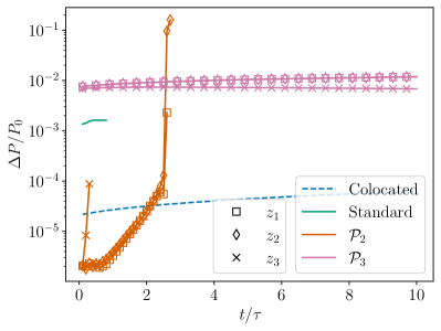
(a) Temporal variation of $\Delta P$.

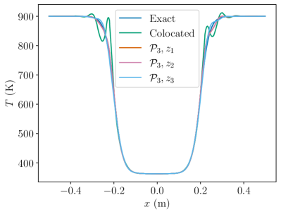
(b) Temperature profiles at $t=10\tau$.

Figure 3.1: Solution to the advection of a nitrogen/n-dodecane thermal bubble at $v=1\text{ m/s}$. Figure 3.1a shows the temporal variation of $\Delta P$, sampled at intervals of $\tau/10$ (for a total of 100 samples if the solution does not diverge). For the $\mathcal{P}_{3}$ results, only every fourth marker is shown. Figure 3.1b displays the temperature profiles at $t=10\tau$ for the stable solutions.

3.2 High velocity, $v=600\text{ m/s}$

As in the previous subsection, Figure 3.2a displays the temporal variation of $\Delta P$ for the considered approaches. The $\mathcal{P}_{2}$ solutions again initially exhibit very small pressure oscillations before diverging, with the $z_{3}$ case diverging most rapidly. Furthermore, when using $\mathcal{P}_{3}$, $z_{3}$ again gives smaller deviations from pressure equilibrium than $z_{1}$ and $z_{2}$. However, key differences with the low-velocity case are observed. First, the magnitude of pressure oscillations is generally greater in the high-velocity case, although the $\mathcal{P}_{3}$ solutions yield deviations of similar magnitude between both velocities. Second, standard overintegration maintains stability throughout the simulation. Additionally, of the stable solutions, the colocated case exhibits the largest pressure deviations, which would likely continue to grow if the simulation is run for longer times. In contrast, the maximum pressure deviations for the other stable solutions seem to have either plateaued or begun to plateau. Pressure equilibrium is the most well-preserved in the $\mathcal{P}_{3}$ solutions, particularly in conjunction with $z_{3}$.

Figure 3.2b presents the temperature profiles of the stable solutions at $t=10\tau$. Temperature oscillations are observed in the cases of colocated integration and standard overintegration. In contrast, the $\mathcal{P}_{3}$ solutions exhibit better agreement with the exact temperature.

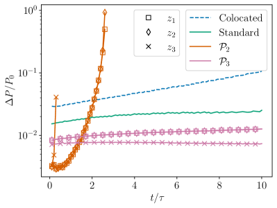
(a) Temporal variation of $\Delta P$.

(b) Temperature profiles at $t=10\tau$.

Figure 3.2: Solution to the advection of a nitrogen/n-dodecane thermal bubble at $v=600\text{ m/s}$. Figure 3.2a shows the temporal variation of $\Delta P$, sampled at intervals of $\tau/10$ (for a total of 100 samples if the solution does not diverge). For the $\mathcal{P}_{3}$ results, only every fourth marker is shown. Figure 3.2b displays the temperature profiles at $t=10\tau$ for the stable solutions.

To help explain why overintegration with $\mathcal{P}_{3}$ can lead to higher solution stability than both standard overintegration (i.e., $\mathcal{P}_{1}$) and overintegration with $\mathcal{P}_{2}$, we take the $\mathcal{P}_{1}$ solution at $t=10\tau$ and then evaluate the pressure in the cell $\kappa=\left[-0.22,-0.2\right]\text{ m}$ with the $\mathcal{P}_{1}$, $\mathcal{P}_{2}$, and $\mathcal{P}_{3}$ projection operators. The resulting pressure-deviation profiles in the given cell are displayed in Figure 3.3. Noticeable pressure deviations are located at the faces in the $\mathcal{P}_{1}$ case (i.e., the pressure is evaluated normally); since $\mathcal{P}_{2}$ (at least using Gauss-Lobatto points) does not modify pressure at the faces, overall deviation from pressure equilibrium is not appreciably reduced. In contrast, $\mathcal{P}_{3}$ markedly improves preservation of pressure equilibrium throughout the cell, indicating that $L^{2}$-projection can act as a mechanism to reduce spurious oscillations that initially emerge via, for instance, underresolution or inexact evaluation of the flux. In the case of $z_{2}$ or $z_{3}$, oscillations of other variables can also be mitigated. However, it should be noted that $\mathcal{P}_{2}$ can reduce pressure oscillations if deviations are large inside the cell but not at the faces. Furthermore, there is no guarantee that $\mathcal{P}_{3}$ will always reduce spurious oscillations.

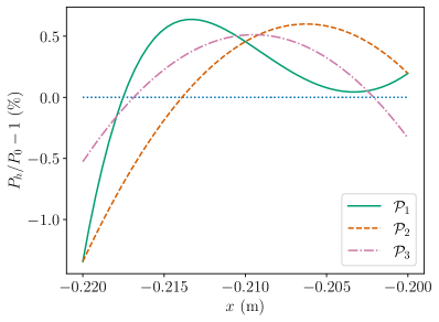
Figure 3.3: Pressure-deviation profiles in the cell $\kappa=\left[-0.22,-0.2\right]\text{ m}$ evaluated with the $\mathcal{P}_{1}$, $\mathcal{P}_{2}$, and $\mathcal{P}_{3}$ projection operators for the $\mathcal{P}_{1}$ solution at $t=10\tau$. The dotted blue line corresponds to exact pressure equilibrium.

4 Concluding remarks

In this short note, we reevaluated previously introduced techniques designed to reduce spurious pressure oscillations at contact interfaces in multicomponent flows in the context of overintegrated DG discretizations [12, 15]. Specifically, we focused on strategies that do not (a) introduce conservation error, (b) rely on artificial viscosity or limiting, or (c) degrade order of accuracy in smooth regions of the flow. The considered techniques, which employ a projection of the pressure (and potentially additional variables) onto the finite element trial space via either interpolation or $L^{2}$-projection, were previously shown to maintain approximate pressure equilibrium and thus stable solutions over long times (in contrast to a standard DG scheme with overintegration) in the advection of a hydrogen/oxygen thermal bubble. In [12], interpolation-based projection was considered the preferred approach due to better preservation of pressure equilibrium.

In this work, we considered a more challenging test case: advection of a high-pressure nitrogen/n-dodecane thermal bubble at both low and high velocities. All simulations were performed on a 50-cell grid using $p=2$. Key observations from this test case are as follows:

• Interpolation-based projection always led to solver divergence. Although it overall maintained stability for longer times than standard overintegration in the low-velocity case, it was outperformed by standard overintegration in the high-velocity case.

• $L^{2}$-projection always maintained solution stability. It produced larger pressure deviations than colocated integration in the low-velocity case but more effectively maintained pressure equilibrium than all other approaches in the high-velocity case.

• Performing $L^{2}$-projection of a full set of primitive variables (specifically, mass fractions, pressure, temperature, and velocity) more effectively preserved pressure equilibrium than if only pressure or if both pressure and velocity were projected. However, projecting a smaller set of variables may be sufficient for stability.

• $L^{2}$-projection led to better predictions of temperature than colocated integration and standard overintegration.

• Colocated integration always maintained solution stability, but led to inferior temperature predictions, indicating that higher resolution (than in the case of overintegration) may be needed to offset the greater integration error.

These findings suggest that this configuration is more effective at testing the ability of a numerical scheme to preserve pressure equilibrium, even without consideration of a cubic equation of state or more complicated thermodynamic relations commonly associated with it [17, 18]. Furthermore, it is also valuable to consider different advection velocities. It should be also be noted that although the $L^{2}$-projection-based approach is the only overintegration strategy that prevented solver divergence across all considered conditions, the interpolation-based approach is simpler and was shown to maintain robustness across a variety of challenging test cases involving more realistic flow conditions and geometries, including moving detonation waves and a chemically reacting shear layer [12], suggesting that it may still be a reliable choice.

Future work will involve consideration of real-fluid effects, in particular a cubic equation of state and thermodynamic departure functions [17], in multiple dimensions. The ability of the considered techniques, specifically the $L^{2}$-projection-based strategy, will be further assessed in this more challenging context of transcritical and supercritical flows. Furthermore, a fully conservative finite volume scheme that mathematically guarantees preservation of pressure equilibrium was recently developed by Fujiwara et al. [24]; an extension to DG schemes may indeed be worth pursuing.

References

- [1] R. Abgrall, Generalisation of the Roe scheme for the computation of mixture of perfect gases, La Recherche Aérospatiale 6 (1988) 31–43.
- [2] S. Karni, Multicomponent flow calculations by a consistent primitive algorithm, Journal of Computational Physics 112 (1) (1994) 31 – 43. doi:https://doi.org/10.1006/jcph.1994.1080.
- [3] R. Abgrall, How to prevent pressure oscillations in multicomponent flow calculations: A quasi conservative approach, Journal of Computational Physics 125 (1) (1996) 150 – 160. doi:https://doi.org/10.1006/jcph.1996.0085.
- [4] A. Gouasmi, K. Duraisamy, S. M. Murman, Formulation of entropy-stable schemes for the multicomponent compressible Euler equations, Computer Methods in Applied Mechanics and Engineering 363 (2020) 112912.
- [5] R. Abgrall, S. Karni, Computations of compressible multifluids, Journal of Computational Physics 169 (2) (2001) 594 – 623. doi:https://doi.org/10.1006/jcph.2000.6685.
- [6] W. H. Reed, T. Hill, Triangular mesh methods for the neutron transport equation, Tech. rep., Los Alamos Scientific Lab., N. Mex.(USA) (1973).
- [7] F. Bassi, S. Rebay, High-order accurate discontinuous finite element solution of the 2D Euler equations, Journal of Computational Physics 138 (2) (1997) 251–285.
- [8] B. Cockburn, G. Karniadakis, C.-W. Shu, The development of discontinuous Galerkin methods, in: Discontinuous Galerkin Methods, Springer, 2000, pp. 3–50.
- [9] G. Billet, J. Ryan, A Runge–Kutta discontinuous Galerkin approach to solve reactive flows: The hyperbolic operator, Journal of Computational Physics 230 (4) (2011) 1064 – 1083. doi:https://doi.org/10.1016/j.jcp.2010.10.025.
- [10] Y. Lv, M. Ihme, Discontinuous Galerkin method for multicomponent chemically reacting flows and combustion, Journal of Computational Physics 270 (2014) 105 – 137. doi:https://doi.org/10.1016/j.jcp.2014.03.029.
- [11] K. Bando, M. Sekachev, M. Ihme, Comparison of algorithms for simulating multi-component reacting flows using high-order discontinuous Galerkin methods (2020). doi:10.2514/6.2020-1751.
- [12] R. F. Johnson, A. D. Kercher, A conservative discontinuous Galerkin discretization for the chemically reacting Navier–Stokes equations, Journal of Computational Physics 423 (2020) 109826. doi:10.1016/j.jcp.2020.109826.
- [13] E. J. Ching, R. F. Johnson, A. D. Kercher, Positivity-preserving and entropy-bounded discontinuous Galerkin method for the chemically reacting, compressible Euler equations. Part II: The multidimensional case, arXiv preprint arXiv:2211.16297 https://arxiv.org/abs/2211.16297 (2022).
- [14] E. J. Ching, R. F. Johnson, A. D. Kercher, Positivity-preserving and entropy-bounded discontinuous Galerkin method for the chemically reacting, compressible Euler equations. Part I: The one-dimensional case, arXiv preprint arXiv:2211.16254 https://arxiv.org/abs/2211.16254 (2022).
- [15] K. Bando, Towards high-performance discontinuous Galerkin simulations of reacting flows using Legion, Ph.D. thesis, Stanford University (2023).
- [16] N. Franchina, M. Savini, F. Bassi, Multicomponent gas flow computations by a discontinuous Galerkin scheme using L2-projection of perfect gas EOS, Journal of Computational Physics 315 (2016) 302–322.
- [17] P. C. Ma, Y. Lv, M. Ihme, An entropy-stable hybrid scheme for simulations of transcritical real-fluid flows, Journal of Computational Physics 340 (2017) 330–357.
- [18] B. Boyd, D. Jarrahbashi, A diffuse-interface method for reducing spurious pressure oscillations in multicomponent transcritical flow simulations, Computers & Fluids 222 (2021) 104924.
- [19] H. Atkins, C. Shu, Quadrature-free implementation of discontinuous Galerkin methods for hyperbolic equations, ICASE Report 96-51, 1996, Tech. rep., NASA Langley Research Center, nASA-CR-201594 (August 1996).
- [20] H. L. Atkins, C.-W. Shu, Quadrature-free implementation of discontinuous Galerkin method for hyperbolic equations, AIAA Journal 36 (5) (1998) 775–782.
- [21] E. Toro, Riemann solvers and numerical methods for fluid dynamics: A practical introduction, Springer Science & Business Media, 2013.
- [22] S. Gottlieb, C. Shu, E. Tadmor, Strong stability-preserving high-order time discretization methods, SIAM review 43 (1) (2001) 89–112.
- [23] A. Corrigan, A. Kercher, J. Liu, K. Kailasanath, Jet noise simulation using a higher-order discontinuous Galerkin method, in: 2018 AIAA SciTech Forum, 2018, AIAA-2018-1247.
- [24] Y. Fujiwara, Y. Tamaki, S. Kawai, Fully conservative and pressure-equilibrium preserving scheme for compressible multi-component flows, Journal of Computational Physics 478 (2023) 111973.