Utilizing Language Models for Energy Load Forecasting

Abstract.

Energy load forecasting plays a crucial role in optimizing resource allocation and managing energy consumption in buildings and cities. In this paper, we propose a novel approach that leverages language models for energy load forecasting. We employ prompting techniques to convert energy consumption data into descriptive sentences, enabling fine-tuning of language models. By adopting an autoregressive generating approach, our proposed method enables predictions of various horizons of future energy load consumption. Through extensive experiments on real-world datasets, we demonstrate the effectiveness and accuracy of our proposed method. Our results indicate that utilizing language models for energy load forecasting holds promise for enhancing energy efficiency and facilitating intelligent decision-making in energy systems.

1. Introduction

With the increasing need for energy efficiency and sustainable resource management, the forecasting of energy load has become a critical requirement in buildings, cities, and transportation systems. Accurate load forecasting enables proactive resource allocation, optimal demand response, and efficient energy management. Traditional approaches to energy load forecasting typically rely on statistical models and recent deep learning-based time series analysis techniques. In recent years, language models based on deep learning, particularly Transformer-based models, have shown remarkable performance in various natural language processing tasks. These models have the ability to learn rich representations of textual data and capture intricate relationships between words and concepts. Typically, the forecasting process of these deep learning models involves one encoder that takes a sequence of numbers that stands for the historical energy consumption values as input and one decoder to generate another sequence of numerical values as the predicted future energy data, as illustrated in Figure 1 (a).

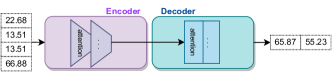
(a) Typical numerical-based forecasting

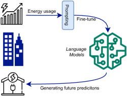
(b) The proposed language-based forecasting

Figure 1. The concept illustration of: (a) the numerical-based deep learning forecasting methods; and (b) the proposed approach of using language models to forecast energy load.

Motivated by the success of language models in natural language processing, we propose to leverage their power for energy load forecasting. As demonstrated in Figure 1 (b), the core of our approach is converting energy consumption data into natural language sentences using prompting techniques. By describing the data as sentences, we aim to unlock the potential of language models to capture nuanced patterns and dependencies within the data. This representation allows us to fine-tune pre-trained language models, enabling them to learn from the specific characteristics of energy consumption sequences. Similar numerical prompting has been used for human mobility data (Xue et al., 2022a, b) recently. However, their prompts only support the forecasting of the next time step, which is limited for predicting the future energy load. To this end, we further introduce an autoregressive mechanism in the prediction generation process with the fine-tuned language models. This approach allows us to generate predictions for different horizons, ranging from short-term (e.g., the next time step) to long-term (e.g., the next 24 time steps) load forecasts.

Our method presents a novel “code less” solution for energy load forecasting, which could provide a new perspective rather than focusing on designing complicated deep learning forecasting models (e.g., Transformer-based methods). This would makes it a relatively easy-accessible and user-friendly method for non-AI users, compared to existing forecasting models that require many tedious parameter searching and training processes. In summary, our main contributions in this work are twofold: (1) We present a study on the utilization of language models for energy load forecasting. We design a pipeline that converts the energy consumption data into sentences for fine-tuning the language models and leverages the autoregressive mechanism for predicting different horizons with the same fine-tuned model. (2) We provide a comprehensive evaluation of the proposed solution with real world data from 6 buildings. We also conduct different evaluation settings including zero-shot performance evaluation and varied prediction horizon evaluation.

2. Forecasting with Language Models

2.1. Problem Formulation and Method Overview

Assume that the energy consumption records of a building $i$ is represented by a sequence of $t$ continuous time steps $\mathcal{X}^{i}=\{x_{1}^{i},x_{2}^{i},\cdots,x_{t}^{i}\}$. The value indicates that the energy consumption of building $i$ at time $t$ is $x_{t}^{i}$. The energy load forecasting problem can then be formulated as predicting the future load consumption values $y^{i}_{t_{1}:t_{m}}$ of the next $m$ time steps given the history observation $x^{i}_{t_{1}:t_{n}}$. Here, $n$ and $m$ are the observation length and the prediction horizon.

Overall, as illustrated in Figure 1 (b), the proposed method comprises three key enablers: (1) Prompting: to transform the raw consumption data into sentences that can be processed by language models; (2) Fine-tuning language models: to adapt them to the specifics of energy forecasting task; (3) Autoregressive generation: to enable the generation of multiple future steps forecasting.

2.2. Prompting and Fine-tuning

To utilize language models for energy load forecasting, we employ a prompting technique that translates the usage data. Generally, the raw energy data is provided in a tabular format and we translate each row into a descriptive sentence. The objective is to transform the raw numerical data into a natural language text format that is suitable for language models and captures the relevant information and context necessary for predictions. By converting the energy consumption data into sentences, language models are enabled to take the transformed energy data as input and capture nuanced patterns and dependencies within the data.

In the prompting process, we utilize a predefined template (e.g., “The electric load at {Time} is {Usage}.”) that serves as a backbone for constructing the sentences. The template consists of placeholders for the actual values from the data, resulting in sentences that convey the energy consumption information in a human-readable format. The template includes variables such as date, time, energy consumption, and any other metadata provided in the raw data that may be relevant for forecasting. By replacing the placeholders in the template with the actual values, we obtain a sentence that represents the energy consumption data for a particular time step. This process is repeated for each row in the raw tabular data, resulting in a collection of descriptive sentences that are used for fine-tuning the language models. Through prompting, we bridge the gap between numerical energy consumption data and the language model’s ability to comprehend and generate textual information.

After generating the sentences from the energy consumption data, we proceed to fine-tune a pre-trained language model. Fine-tuning allows the model to adapt to the specific characteristics of load forecasting and capture the dependencies within the data. The language models are often pre-trained on a large corpus of text data to learn general language representations and common knowledge. In this study, we leverage the pre-trained models provided by HuggingFace and the models are pre-trained only with general English-language corpora datasets without any specific energy usage-related numerical datasets. Fine-tuning involves training the language model on our generated load sentences to specialize it for load forecasting. During the fine-tuning process, we feed the generated sentences as input to the language models and optimize the parameters to minimize the difference between the predicted next sentence and the ground truth sentence. This process could make the language models suitable for our load forecasting task.

2.3. Autoregressive Generation

Taking a set of historical sentences representing past energy load consumption as input, the fine-tuned language models generate the next sentence, which corresponds to the predicted energy load for the next time step. When longer prediction horizons are required, we adopt an autoregressive method and we extend the prediction horizon by appending the generated sentence to the end of the input sentence sequence. This extended sequence becomes the input for predicting the subsequent time step. By iteratively generating sentences in an autoregressive manner, we can forecast energy load consumption for multiple future time steps.

The autoregressive generation approach leverages the fine-tuned language model’s ability to capture dependencies between historical consumption and future load patterns. By using the generated sentences as input, the model can adjust its predictions based on the evolving context, enabling dynamic forecasts for different horizons.

3. Experiments

3.1. Dataset and Evaluation

This study uses data from a certain block within the Melbourne CBD area in Australia. We select aggregated and anonymised smart meter data of hourly energy consumption for 6 buildings (i.e., Building A-F). The data is collected from 2018 January to 2019 December. For each building, the data of the first 22 months is considered as the training set to fine-tune the language models. The data of the last month (Dec. 2019) is used as the testing set and the remaining month (Nov. 2019) is split as the validation set.

Table 1. The comparison between numerical forecasting methods and the proposed forecasting with language models.

	Building A		Building B		Building C		Building D		Building E		Building F
	RMSE	MAE	RMSE	MAE	RMSE	MAE	RMSE	MAE	RMSE	MAE	RMSE	MAE
Transformer	143.383	110.462	6.022	3.966	47.671	30.051	18.008	12.932	6.950	4.735	37.636	26.628
Informer	176.335	135.877	5.127	3.274	45.660	28.253	17.557	12.408	5.999	4.194	35.066	24.261
Autoformer	60.703	41.873	5.521	3.891	54.415	38.463	26.603	18.902	8.335	6.142	45.291	34.578
FEDformer	50.055	32.488	5.455	3.772	48.001	33.619	27.548	20.789	7.882	5.879	44.008	33.883
Language Model-based (ours)
Bart	28.634	20.489	3.266	1.871	33.635	25.050	48.555	28.074	4.308	2.793	28.734	20.990
Bigbird	28.350	19.181	4.617	2.803	25.466	19.903	34.831	19.235	4.402	2.988	28.509	21.237
Pegasus	20.419	15.124	3.186	1.865	29.453	22.201	53.986	32.419	5.161	3.201	28.434	21.298

Table 2. Results of language models under the zero-shot setting.

Fine-tuning data		Building B		Building C		Building D		Building E		Building F
		RMSE	MAE	RMSE	MAE	RMSE	MAE	RMSE	MAE	RMSE	MAE
	Bart	49.645	9.780	53.534	40.466	18.154	12.276	142.760	65.407	60.022	43.923
Building A	Bigbird	140.140	104.256	34.929	24.990	20.014	13.028	193.763	183.637	51.590	36.235
	Pegasus	71.213	39.008	27.545	21.400	22.655	15.344	178.871	140.538	40.983	32.209
		Building A		Building C		Building D		Building E		Building F
	Bart	265.186	258.663	223.216	215.495	121.805	116.927	10.050	7.318	275.279	262.617
Building B	Bigbird	245.885	239.373	207.996	199.670	115.281	104.371	6.404	4.189	255.267	241.459
	Pegasus	209.142	180.299	182.130	158.734	107.290	95.584	5.568	4.053	222.276	192.440
		Building A		Building B		Building D		Building E		Building F
	Bart	31.098	24.549	11.771	4.609	121.081	100.328	52.622	15.383	40.697	30.991
Building C	Bigbird	31.565	25.242	16.049	4.201	53.462	37.821	147.580	97.219	36.477	27.524
	Pegasus	31.859	25.333	11.736	6.661	79.377	64.420	10.332	5.932	35.590	27.711
		Building A		Building B		Building C		Building E		Building F
	Bart	103.643	77.086	60.994	21.930	68.729	49.655	90.899	48.022	134.490	95.149
Building D	Bigbird	37.347	26.154	85.492	49.806	36.092	26.142	182.591	168.000	68.114	49.591
	Pegasus	57.576	41.751	35.009	10.887	47.066	35.939	76.964	28.347	82.010	59.684
		Building A		Building B		Building C		Building D		Building F
	Bart	246.991	239.025	9.345	7.148	204.619	195.582	97.547	89.958	258.007	243.845
Building E	Bigbird	251.074	245.359	34.759	27.898	211.649	203.910	82.280	63.093	260.483	247.872
	Pegasus	240.030	228.999	9.827	4.740	192.677	170.909	70.708	51.297	251.381	232.470
		Building A		Building B		Building C		Building D		Building E
	Bart	40.445	32.498	15.492	4.670	27.708	20.957	55.216	35.233	56.668	15.612
Building F	Bigbird	34.152	27.685	11.730	3.715	26.631	20.123	28.173	18.846	162.201	113.104
	Pegasus	39.271	32.015	7.077	3.802	30.097	23.107	38.075	25.148	12.781	6.263

For evaluating the performance of each method, we use the Root Mean Squared Error (RMSE) and the Mean Absolute Error (MAE) as metrics. For both the measures, the lower error means the better performance. These errors are calculated based on the predicted $\hat{y}_{t_{1}:t_{m}}^{i}$ and the ground truth $y_{t_{1}:t_{m}}^{i}$ to measure the closeness of the predicted values. For this study, we have fixed a forecast horizon size of $m=24$ hours, to mimic a day-ahead forecasting experiment. To make the input observation size bigger than the output prediction horizon, we set the input observation length $n=30$.

3.2. Performance

3.2.1. Comparing Against Numerical Forecasting Methods

To evaluate the performance of our approach, we compare it against the typical numerical forecasting methods commonly used for time series forecasting. Specifically, we select the popular Transformer (Vaswani et al., 2017) as well as the more recent Informer (Zhou et al., 2021), Autoformer (Xu et al., 2021), and FEDformer (Zhou et al., 2022) as numerical baselines. For language models, a recent benchmark study (Xue and Salim, 2023) has shown that three language models (Bart (Lewis et al., 2020), Bigbird (Zaheer et al., 2020), and Pegasus (Zhang et al., 2020)) have better forecasting ability. These models also have reasonable size and number of parameters so that they can run on a single GPU (e.g., we used Nvidia V100 in our experiments). Thus, these three language models are selected in our evaluation and our implementations are available at: https://github.com/xuehaouwa/LM-Load-Forecasting.

The best performance under each column is shown in bold in Table 1. From the table, it is evident that language models, with our proposed pipeline, outperform traditional numerical forecasting methods in the majority of cases. Specifically, the language models have superior performance over baselines with a significant gain on Building A, B, C, and F. These findings highlight the language models’ ability to capture patterns within energy consumption data, ultimately leading to more accurate predictions.

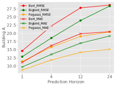
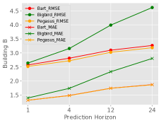
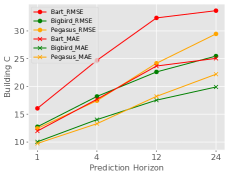
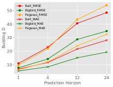
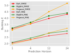
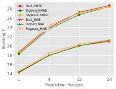
Figure 2. The performance of language models with different prediction horizons.

3.2.2. Zero-shot Performance

In addition to the above evaluation of the language models, we also assess the performance through zero-shot setting. In our study, the zero-shot setting aims to evaluate the ability of the language model to generate reasonable predictions even without fine-tuning on the corresponding training data of one building. Specifically, as listed in Table 2, we fine-tuned the language models with the training set of one building. Instead of using the testing set of the same building, we directly use the fine-tuned model to generate predictions for the testings sets of other buildings. In the table, we highlight the results that achieve similar or even better performance than the results reported in Table 1. As we can see, with our proposed pipeline, the language models can still yield plausible predictions for most of the buildings under the challenging zero-shot setting. This evaluation provides insights into the language model’s ability to generalize and transfer knowledge across different buildings. It also suggests that our proposed approach can be used to achieve reasonable forecasting results even for buildings without specific fine-tuning or buildings without enough recorded data to start with fine-tuning (e.g., cold start situation), which highlights the versatility and potential of language models in energy load forecasting.

3.2.3. Different Prediction Horizons

Furthermore, we investigate the effectiveness of our approach for different prediction lengths. We examine the performance of our method for different prediction lengths to assess its adaptability over varying time scales. Specifically, we set the prediction horizon $m=\{1,4,12,24\}$ and the performance of three language models on 6 buildings are visualized in Figure 2. For each building, the language model is only fine-tuned once (fine-tuned to generate the prediction of the next time step). The same fine-tuned model is used to yield forecasting for different horizons based on our autoregressive generation mechanism. From the figure, although the error increases when the prediction horizon is enlarged (which is as expected), the results show that once the model is fine-tuned, it can be applied to arbitrary forecasting horizons. The adaptability of language models in our forecasting pipeline across varying prediction horizons demonstrates the versatility and suitability of our method for real-world applications where dynamic, multi-step forecasting is essential.

4. Conclusion

We present a novel approach for energy load forecasting that leverages existing language models. Through prompting, fine-tuning language models, and autoregressive prediction mechanism, our method enables accurate and dynamic predictions of energy consumption. We have demonstrated the potential and the good performance of our proposed approach by evaluation with real-world data and comparisons against traditional numerical forecasting methods. The zero-shot evaluation also reveals the ability of language models to generate reasonable predictions even without specific fine-tuning on a particular building. By harnessing the power of language models, our method provides a promising direction to unlock valuable insights for energy forecasting. Future research can focus on exploring prompt optimization to further improve the accuracy and applicability of language models in load forecasting.

References

- (1)
- Lewis et al. (2020) Mike Lewis, Yinhan Liu, Naman Goyal, Marjan Ghazvininejad, Abdelrahman Mohamed, Omer Levy, Veselin Stoyanov, and Luke Zettlemoyer. 2020. BART: Denoising Sequence-to-Sequence Pre-training for Natural Language Generation, Translation, and Comprehension. In Proceedings of the 58th Annual Meeting of the Association for Computational Linguistics, ACL 2020, Online, July 5-10, 2020. Association for Computational Linguistics, 7871–7880.
- Vaswani et al. (2017) Ashish Vaswani, Noam Shazeer, Niki Parmar, Jakob Uszkoreit, Llion Jones, Aidan N Gomez, Łukasz Kaiser, and Illia Polosukhin. 2017. Attention is all you need. Advances in neural information processing systems 30 (2017).
- Xu et al. (2021) Jiehui Xu, Jianmin Wang, Mingsheng Long, et al. 2021. Autoformer: Decomposition transformers with auto-correlation for long-term series forecasting. Advances in Neural Information Processing Systems 34 (2021).
- Xue and Salim (2023) Hao Xue and Flora D. Salim. 2023. PromptCast: A New Prompt-based Learning Paradigm for Time Series Forecasting. arXiv:2210.08964
- Xue et al. (2022a) Hao Xue, Flora D Salim, Yongli Ren, and Charles LA Clarke. 2022a. Translating Human Mobility Forecasting through Natural Language Generation. In Proceedings of the Fifteenth ACM International Conference on Web Search and Data Mining. 1224–1233.
- Xue et al. (2022b) Hao Xue, Bhanu Prakash Voutharoja, and Flora D Salim. 2022b. Leveraging language foundation models for human mobility forecasting. In Proceedings of the 30th International Conference on Advances in Geographic Information Systems.
- Zaheer et al. (2020) Manzil Zaheer, Guru Guruganesh, Kumar Avinava Dubey, Joshua Ainslie, Chris Alberti, Santiago Ontanon, Philip Pham, Anirudh Ravula, Qifan Wang, Li Yang, et al. 2020. Big bird: Transformers for longer sequences. Advances in Neural Information Processing Systems 33 (2020), 17283–17297.
- Zhang et al. (2020) Jingqing Zhang, Yao Zhao, Mohammad Saleh, and Peter Liu. 2020. Pegasus: Pre-training with extracted gap-sentences for abstractive summarization. In International Conference on Machine Learning. PMLR, 11328–11339.
- Zhou et al. (2021) Haoyi Zhou, Shanghang Zhang, Jieqi Peng, Shuai Zhang, Jianxin Li, Hui Xiong, and Wancai Zhang. 2021. Informer: Beyond efficient transformer for long sequence time-series forecasting. In Proceedings of AAAI.
- Zhou et al. (2022) Tian Zhou, Ziqing Ma, Qingsong Wen, Xue Wang, Liang Sun, and Rong Jin. 2022. FEDformer: Frequency Enhanced Decomposed Transformer for Long-term Series Forecasting. In International Conference on Machine Learning, ICML 2022, 17-23 July 2022, Baltimore, Maryland, USA (Proceedings of Machine Learning Research, Vol. 162). PMLR, 27268–27286.