Making the End-User a Priority in Benchmarking: OrionBench for Unsupervised Time Series Anomaly Detection

Sarah Alnegheimish Laure Berti-Equille Kalyan Veeramachaneni

Abstract

Time series anomaly detection is a prevalent problem in many application domains such as patient monitoring in healthcare, forecasting in finance, or predictive maintenance in energy. This has led to the emergence of a plethora of anomaly detection methods, including more recently, deep learning based methods. Although several benchmarks have been proposed to compare newly developed models, they usually rely on one-time execution over a limited set of datasets and the comparison is restricted to a few models. We propose OrionBench – a user centric continuously maintained benchmark for unsupervised time series anomaly detection. The framework provides universal abstractions to represent models, extensibility to add new pipelines and datasets, hyperparameter standardization, pipeline verification, and frequent releases with published benchmarks. We demonstrate the usage of OrionBench, and the progression of pipelines across 15 releases published over the course of three years. Moreover, we walk through two real scenarios we experienced with OrionBench that highlight the importance of continuous benchmarks in unsupervised time series anomaly detection.

Machine Learning, ICML

1 Introduction

Table 1: Latest published results in each benchmarking framework. These frameworks are point-in-time benchmarks lacking continuous runs.

Benchmark Framework	Last Updated	Source
	Published Leaderboard
Numenta (Lavin & Ahmad, 2015)	Jun 2018	Github
TSB UAD (Paparrizos et al., 2022)	Nov 2022	Github
TODS (Lai et al., 2021)	Jan 2021	Paper
TimeEval (Wenig et al., 2022)	Aug 2022	Paper
Exathlon (Jacob et al., 2020)	Sep 2021	Paper
Merlion (Bhatnagar et al., 2021)	Sep 2021	Paper
OrionBench	Aug 2023	Github

As continuous data collection becomes more popular across domains, there is a corresponding need to monitor systems, devices, and even human health and activity in order to find patterns, as well as deviations from those patterns (Chandola et al., 2009; Aggarwal & Aggarwal, 2017). Over the past decade, tremendous progress has been made in using machine learning to perform this monitoring given their generative capabilities, which is known as unsupervised time series anomaly detection. For example, in just the past 5 years, Hundman et al. (2018) created a forecasting LSTM model to find anomalies in spacecraft data, Park et al. (2018) used LSTM variational autoencoders for anomaly detection in multimodal sensor signals collected from robotic arms, and Geiger et al. (2020) used generative adversarial networks for time series anomaly detection on widely used public datasets.

When end-users, who we specifically define as people who are interested in training a model on their data to find anomalies, attempt to use these models, they regularly end up with a few questions. First, “am I using the state-of-art (SOTA) model, and how do I know that?” Second, with rapid innovations in the space and new modeling approaches frequently announced and publicized, ”how can I keep up?” Third, if a model is said to be SOTA, “how can I trust that it is, before investing a lot of effort in using it for my data?” The unsupervised nature of the problem accentuates this need, because unlike with predictive modeling, in unsupervised learning there is no ground truth, and it is always possible to monitor one’s systems better. Ultimately, it is important to note that an end-user is only interested in finding the best solution for their particular problem, and does not think about these modeling techniques the same way researchers do.

In recent years, benchmarks have become instrumental in gauging and comparing model performance (Coleman et al., 2019; Han et al., 2022). In this paper, we ask — can benchmarking frameworks also help to alleviate end-users’ concerns? While many time series anomaly detection benchmarks have been introduced (Jacob et al., 2020; Lai et al., 2021; Paparrizos et al., 2022; Lavin & Ahmad, 2015; Wenig et al., 2022), they are not directed toward end-users. More concretely they are usually not kept up-to-date. Table 1 shows the latest published results for each time series anomaly detection benchmark framework, and whether the score board is updated on github and the last updated date. It is usually the practice that these assessments are done once during publications of related papers. Further comparisons are addressed in Section 2. We argue that this makes them point-in-time benchmarking frameworks.

Still, we propose that with a few careful innovations, these benchmarking frameworks can help end-users. With that in mind, in this paper, we propose OrionBench – a user-centric benchmarking framework for unsupervised time series anomaly detection. Three concrete innovations enable us to address end-users’ common concerns:

•

A continuous running system, moving away from point-in-time evaluations.
•

Abstractions that allow us to easily incorporate and assess new models, and isolate the factors that make them better.
•

Seamless integration of latest models into a usable pipeline for end-users.

Why unsupervised learning?

Anomalous events are scarce, rare, and sometimes unknown. End-users search for “anomalies”, however, they are uncertain of what they are looking for and when anomalies occur in their data without an in-depth investigation. With unsupervised learning, the model flags intervals that it finds to be deviating from the expectation. This helps end-users discover events that are likely to be of interest. With supervised learning, models are restricted to only previously labelled events and end-users often struggle to find enough of these labels for a model to make useful predictions. In OrionBench, we focus on unsupervised models.

We highlight the contributions of our framework as: (1) OrionBench is an extensible framework that enables integration of new pipelines and datasets. OrionBench first started with 2 pipelines, but as of now it encompasses 11 pipelines, 24 primitives, 12 public datasets, and 2 custom evaluation metrics. Once integrated into the framework, benchmarked, the pipeline is seamlessly made available to the end-user through an identical API. (2) A continuously ran benchmark with frequent releases. To date, we have 14 benchmark leaderboards over the course of almost three years, starting in September 2020. Our latest release in October 2023 makes for an overall accumulation of 52,966 experiments. We demonstrate the stability and reproduciblity of OrionBench by showcasing the progression of pipeline performances across all releases to date. (3) OrionBench is open-source and publicly available https://github.com/sintel-dev/Orion under MIT license. (4) An end-to-end benchmark executable with a single command. Given a set of pipeline and datasets, the benchmark evaluates the performance of a pipeline on every signal according to time series anomaly detection based metrics. We provide an extensive evaluation where we illustrate qualitative and computational performances of pipelines across all datasets.

In Section 2 of this paper, we compare our framework to existing open-source benchmarks. We detail the components of OrionBench in Section 3 that make it user-centric. Section 4 presents the evaluation of our benchmark framework and two real scenarios where OrionBench was valuable. Lastly, we conclude in Section 5.

2 Related Work

Table 2: Comparison of anomaly detection benchmarks. A (✓) indicates the framework includes an attribute, while an (✗) indicates the attribute is absent. Categories are: #D and #P represent the number of currently available datasets and pipelines respectively; Supported pipelines can include classic pipelines such as ARIMA, Deep Learning (DL) pipelines such as LSTM, and BlackBox (BBox) pipelines that are called externally through an API such as Azure’s AD service; Custom evaluation methods for time series anomaly detection; Whether the benchmark is extensible and can integrate new datasets and pipelines; If the benchmark is being released in periodic fashion with updated leaderboard.

Benchmark	# D	# P	Classic	DL	BBox	Evaluation	Extensible	Periodic
	Available		Pipeline Type
Numenta (Lavin & Ahmad, 2015)	7	4	✓	✗	✗	✓	✓	✗
TSB-UAD (Paparrizos et al., 2022)	18¹¹1Additional synthetic and artificial data is generated in the benchmark.	12	✓	✓	✗	✓	✗	✗
TODS (Lai et al., 2021)	4¹¹1Additional synthetic and artificial data is generated in the benchmark.	9	✓	✓	✗	✗	✗	✗
TimeEval (Wenig et al., 2022)	23	71	✓	✓	✗	✗	✓	✗
Exathlon (Jacob et al., 2020)	10²²2Data are traces from 10 distributed streaming jobs on a Spark cluster.	3	✗	✓	✗	✓	✗	✗
Merlion (Bhatnagar et al., 2021)	12	12	✓	✓	✗	✓	✗	✗
OrionBench	12	11	✓	✓	✓	✓	✓	✓

2.1 Time Series Anomaly Detection Algorithms

Many anomaly detection methods have emerged in the past few years (Chandola et al., 2009; Blázquez-García et al., 2021; Goldstein & Uchida, 2016). These include statistical thresholding techniques (Patcha & Park, 2007), clustering based methods (Münz et al., 2007; Syarif et al., 2012; Agrawal & Agrawal, 2015), and machine learning models (Hasan et al., 2019; Liu et al., 2015). More recently, deep learning models have become popular and have been adopted for anomaly detection (Chalapathy & Chawla, 2019; Pang et al., 2021). Deep learning based anomaly detection models for time series data rely mostly on unsupervised learning, because in most settings there is no a priori knowledge of anomalous events. Malhotra et al. (2016) built an autoencoder with Long Short-Term Memory (LSTM) layers (Hochreiter & Schmidhuber, 1997) that learns to reconstruct ‘normal’ signal behavior. It uses the residual between the reconstructed signal and the original signal to locate anomalies. LSTM networks are practical at capturing the temporal dynamics in time series data. Hundman et al. (2018) used an LSTM forecasting model to predict the signal and paired it with a non-parametric threshold to mitigate false positives. Many variations on the same principle exist, including variational autoencoders (VAE) (Park et al., 2018), and Generative Adversarial Networks (GAN) (Geiger et al., 2020).

2.2 Time Series Anomaly Detection Benchmarks

There are several notable open-source time series benchmarking systems featuring unsupervised time series anomaly detection methods (Lavin & Ahmad, 2015; Paparrizos et al., 2022; Lai et al., 2021; Wenig et al., 2022; Jacob et al., 2020; Bhatnagar et al., 2021). Table 2 highlights the key features present in each framework. In addition to unsupervised pipelines, some frameworks include supervised pipelines (Paparrizos et al., 2022; Wenig et al., 2022). However, comparing supervised pipelines to unsupervised ones can be misleading, as labels are not available in most real-world scenarios. We address three key points with OrionBench (1) time series anomaly detection requires careful consideration of how to evaluate pipelines; (2) integration of new pipelines and datasets needs to be seamless such that pipelines can be available to end-users, (3) benchmarks need periodic releases and leaderboard updates to ensure results are trusted and pipelines are stable.

There are many other benchmarking frameworks, such as time series forecasting benchmarks (Alexandrov et al., 2020; Bauer et al., 2021; Taieb et al., 2012), and anomaly detection for tabular data (Campos et al., 2016; Han et al., 2022). However, these benchmarks naturally differ from our unsupervised anomaly detection benchmark for time series data.

3 System Overview

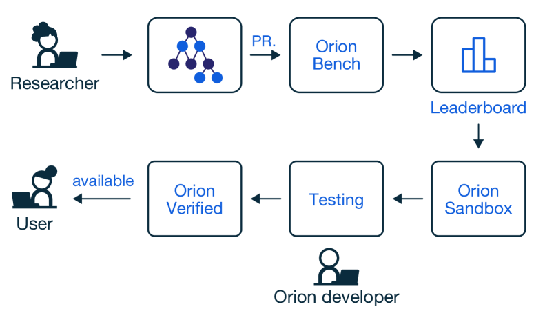
Refer to caption — Figure 1: User centric benchmarking framework

OrionBench is a benchmark suite within the Orion system (Alnegheimish, 2022). A researcher creates a new model and integrates it with Orion through a pull request. A benchmark run is executed and produces a leaderboard, and the model is then stored in the sandbox. This part of the workflow satisfies the goals of the researcher. To serve end-users, pipelines in the sandbox are tested by an Orion developer. Those pipelines that pass the tests are verified and become available to end-users. This workflow is depicted in Figure 1. Five main properties enable our framework for benchmarking unsupervised time series anomaly detection models: abstractions that enable us to compose models as pipelines (directed acyclic graphs) of resusable components called primitives; extensions to add new pipelines and datasets; hyperparameter standardization; verification of pipelines; and continuous benchmark releases.

3.1 Model Abstractions into Primitives and Pipelines

New unsupervised time series anomaly detection models are constantly being developed. This poses the question: how do we represent all such models in a uniform way?

To accomplish this goal, we standardize models. The anomaly detection process starts with a signal $\mathbf{X}=\{\mathbf{x}_{1},\mathbf{x}_{2},\dots,\mathbf{x}_{T}\}$ where $T$ is the length of the time series and $\mathbf{x}_{i}\in\mathbb{R}^{n}$ and $n$ is the number of channels. When the time series is a univariate signal then $n=1$ . The goal is to find a set of anomalous intervals $A=\{(t_{s}^{1},t_{e}^{1}),\dots,(t_{s}^{k},t_{e}^{k})\}$ where $k\geq 0$ . Each interval represents the start and end timestamps of the detected anomaly.

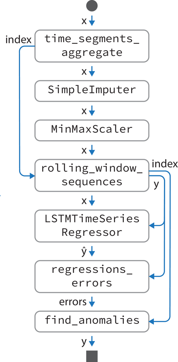
We adopt a universal representation of primitives and pipelines (Smith et al., 2020). Primitives are reusable basic block components that perform a single operation. Primitives can be single tasks, ranging from data scaling, to signal processing, to model training. When primitives are stacked together, they compose pipelines. A pipeline is computed into its respective computational graph, similar to the LSTM DT pipeline and its primitives shown in Figure 2(a), where the input is a uni– or multi-variate time series, and the output is a list of intervals of the detected anomalies. As portrayed in Figure 2(b), we use fit method to train the model and detect method to run inference. With this standardization, we are able to treat all models equivalently. Moreover, primitives provide a code-efficient structure such that we can be modular and re-use primitives between pipelines.

3.2 Extensibility to Integrate New Pipelines and Datasets

One of the main pillars of open-source development is continuously maintaining and updating a library. Benchmark libraries are no different. For the library to grow, it is essential to keep introducing new pipelines and datasets to benefit the end-user.

Contributors build new primitives and compose new pipelines easily in OrionBench . The framework provides templates to help guide contributors in this process (Figure 8 in Appendix). Moreover, contributors can utilize primitives in other packages given a corresponding json representation. They can also use readily available primitives within their pipelines (Smith et al., 2020). It is often the case that pre- and post- processing primitives are reusable across pipelines (Alnegheimish et al., 2022). OrionBench first started with 2 pipelines, and now it has 11 pipelines. The same applies to benchmark datasets. To make the data more accessible, we host publicly available datasets on an Amazon S3 instance. Signals can be loaded via load_signal command (as shown in Figure 2(b)) that will directly connect to S3 if the data is hosted there. Otherwise, it will search for the file locally.

3.3 Hyperparameter Standardization

Deep learning models require setting a multitude of hyperparameters. Moreover, each model contains hyperparameters that are model-specific. This has made it more challenging to keep benchmarks fair and transparent. In OrionBench , hyperparameters are stored as json files with their configuration settings. With a json format, hyperparameters are exposed in both machine- and human- readable representations (Smith et al., 2020). Figure 2(c) is an example of the hyperparameter settings for the LSTM DT pipeline.

To increase benchmark fairness, we standardize hyperparameters for both global and local hyperparameters. Global hyperparameters are shared between pipelines. They typically pertain to to pre- and post- processing primitives. For example, in Figure 2(c), interval is a global hyperparameter that denotes the aggregation level for the signal – here it is set to 6 hours of aggregation (21600 seconds). Such hyperparameters are selected based on the characteristics of the dataset, and in some cases are dynamic. For example, window_size_perc sets the window size of the function to be 30% of the length of the received signal. Local hyperparameters such as epochs are pipeline specific and are selected based on the authors’ recommendation in the original paper. These hyperparameters are consistent across datasets per pipeline in order to alleviate any bias introduced by knowing the ground truth anomalies of the dataset.

OrionBench is specifically made for unsupervised time series anomaly detection As suggested in (Alnegheimish et al., 2022), hyperparameter tuning can be introduced in unsupervised learning by improving the underlying model (e.g. LSTMTimeSeriesRegressor) to forecast a signal that highly resembles the original one by tuning the hyperparameters to minimize metrics such as mean squared error. However, such procedures can overfit the signals to anomalies which precludes subsequent primitives from finding these anomalies, impairing the pipeline’s performance. As such hyperparameter tuning is not currently introduced within the benchmark.

3.4 Verification of Pipelines

We organize pipelines into verified pipelines and sandbox pipelines. When a new pipeline is proposed, it is categorized under ”sandbox” until several tests and validations are made. The researcher opens a new pull request and is requested to pass unit and integration tests before the pipeline is merged and stored in the sandbox. Next, Orion developers test the new pipeline and verify its performance and reproducibility. One of the most commonly encountered situations is mismatch between the researchers report of comparison and the results and Orion developer would get, running the same framework. A very common reason, we found, is that researchers had a hyperparameter setting that they did not update. Once these checks are made, pipelines are transferred from ”sandbox” to ”verified.” The increased reliability of verified pipelines enhances the end-user’s confidence in adopting pipelines.

3.5 Continuous Releases

The last property that advocates for OrionBench is to answer the question: how do benchmarks progress with time? Most pipelines are stochastic in nature, meaning benchmark results can change from run to run. Moreover, when the underlying dependency packages (e.g. TensorFlow, pytorch, etc.) introduce new versions, the pipelines change, and benchmark results can be affected, or even compromised. Therefore, it is crucial to monitor the progression of pipeline performances over time and prevent possible pipeline breakdowns due to backwards incompatibility.

This need is a main driver behind the creation of OrionBench. Benchmarking was introduced as a measure of stability testing, analogous to how Continuous Integration (CI) tests have greatly increased the reliability of open-source libraries. OrionBench now serves as a test of pipeline stability over time. As of now, 15 releases have been published, and the leaderboard changes with each release (see Section 4.2).

4 Evaluation

We demonstrate the use of OrionBench on 11 pipelines and 12 datasets. We also present how benchmarking works as a mechanism to test pipeline stability. Lastly, we present two real-world scenarios where OrionBench was used to ground unsupervised anomaly detection.

Datasets. Currently, the benchmark is executed on 12 datasets with ground truth anomalies. These datasets are gathered from different sources, including NASA ¹¹1https://github.com/khundman/telemanom, NAB ²²2https://github.com/numenta/NAB, Yahoo S5 ³³3https://webscope.sandbox.yahoo.com/catalog.php?datatype=s&did=70, and UCR ⁴⁴4https://www.cs.ucr.edu/~eamonn/time_series_data_2018/UCR_TimeSeriesAnomalyDatasets2021.zip. Collectively, these datasets contain 742 time series and 2,599 anomalies. The properties of the datasets are presented in Table 3. In addition to showing the number of signals and anomalies, we view the average length of the signal and average length of the anomalies in each dataset. Note how the properties of datasets are different: NASA, NAB, and UCR contain anomalies that are longer than Yahoo S5. Moreover, the majority of anomalies in Yahoo S5’s A3 & A4 datasets are point anomalies.

Table 3: Datasets Summary. There are 12 datasets with varying number of signals and anomalies. The table presents the average signal length and anomaly length for each dataset and whether the dataset is real or synthetically generated. All these datasets are publicly accessible.

	Dataset	# Signals	# Anomalies	Avg. Signal	Avg. Anomaly	Synthetic
NASA	MSL	27	36	4890.59	219.58	No
NASA	SMAP	53	67	10618.86	838.07	No
NAB	Art	6	6	4032.00	202.00	Yes
	AWS	17	30	3980.35	105.76	No
	AdEx	5	11	1593.40	73.450	No
	Traf	7	14	2237.71	157.86	No
	Tweets	10	33	15863.1	237.63	No
Yahoo S5	A1	67	178	1415.9	9.37	No
	A2	100	200	1421.0	2.33	Yes
	A3	100	939	1680.0	1.00	Yes
	A4	100	835	1680.0	1.00	Yes
UCR	UCR	250	250	77415.06	196.46	Mixed

Models. As of the writing of this paper, we include 11 pipelines: ARIMA – Autoregressive Integrated Moving Average statistical model (Box & Jenkins, 1968); MP – Discord discovery through matrix profiling (Yeh et al., 2016); AER – AutoEncoder with Regression deep learning model with reconstruction and prediction errors (Wong et al., 2022); LSTM-DT – LSTM non-parametric Dynamic Threshold with two LSTM layers (Hundman et al., 2018); TadGAN – Time series Anomaly Detection using Generative Adversarial Networks (Geiger et al., 2020); LSTM VAE – Variational AutoEncoder with LSTM layers (Park et al., 2018); LSTM AE – AutoEncoder with LSTM layers (Malhotra et al., 2016); Dense AE – Similar to LSTM AE, with Dense layers; GANF – Graph Augmented Normalizing Flows density based model (Dai & Chen, 2022); AnomTransformer – Transformer model with association discrepancy (Xu et al., 2022); Azure AD – Microsoft Azure anomaly detection service (Ren et al., 2019). These pipelines were introduced at different stages of development. Section 4.2 provides further detail on when exactly each model was integrated.

Hyperparameters. Hyperparameter settings are an important part of model performance. As highlighted in Section 3.3, OrionBench seeks to provide a fair benchmark by standardizing hyperparameters. Moreover, we distinguish between all pipelines based on whether they are prediction-based or reconstruction-based (Alnegheimish et al., 2022) and set the hyperparameters based on those properties. The precise values are selected based on the configurations proposed by the original authors in previous work (Hundman et al., 2018; Wong et al., 2022; Geiger et al., 2020; Dai & Chen, 2022). For example, prediction-based pipelines have a large window_size of 250 data points, while reconstruction-based pipelines have a smaller window_size of 100 since the objective is to try and reconstruct the entire window rather than predict a few steps ahead. While some other methods alter the window_size based on the signal length (Malhotra et al., 2016), we provide the option to make these hyperparameters dynamic. For example, window_size can be set as 10% of the entire signal length.

Compute. We setup an instance on MIT supercloud (Reuther et al., 2018) with an Intel Xeon Gold 6249 processor of 10 CPU cores (9 GB RAM per core) and one Nvidia Volta V100 GPU.

⬇

from orion.benchmark import benchmark

pipelines = [ ’arima’, ’lstm_dt’, ’aer’, ’…’]

datasets = [’NAB’, ’NASA’, ’…’]

metrics = [’f1’, ’precision’, ’…’]

benchmark(pipelines=pipelines, datasets=datasets, metrics=metrics, rank=’f1’)

Figure 3: Benchmark command in python. Running benchmark() with default settings will execute the benchmark on all pipelines and datasets currently integrated with the benchmark.

4.1 End-to-End Benchmark

Benchmark Usage. OrionBench is available to all users through a single command, as illustrated in Figure 3. Users specify the list of pipelines, datasets, and metrics they are interested in and pass them to benchmark function. The output result is stored as a detailed .csv file that shows for each pipeline and signals performance metrics such as accuracy, precision, recall, and F1 score. Moreover, it shows the status of the run – whether it was successful or not, total execution time, and the runtime for each internal primitive.

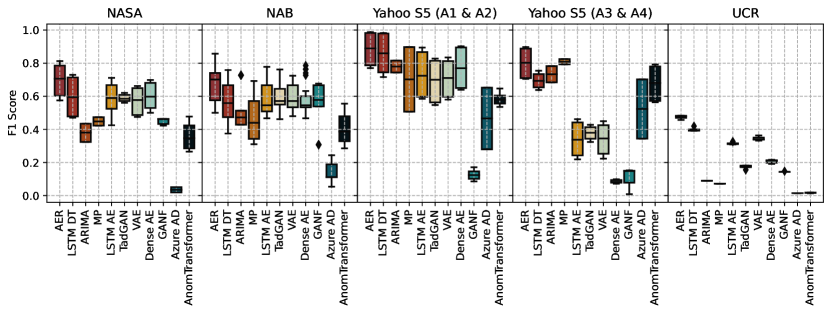
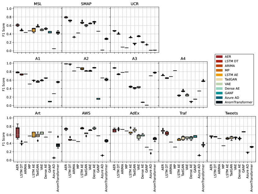
Qualitative Performance. Once we obtain the detailed sheet, we can aggregate the results per pipeline and dataset. Typically, we are interested in the F1 Score; however, users can alter the metric of interest. The final step of the benchmark produces a detailed .csv file that is then summarized to Table 5 in the Appendix. Figure 4 depicts the F1 Score obtained for each dataset on average. We can see that AER is the highest-performing pipeline overall, although LSTM DT competes with AER in some cases. An interesting observation is how LSTM AE, TadGAN, VAE, and Dense AE suffer greatly in detecting point anomalies. The aforementioned pipelines, which are all reconstruction based, are susceptible to anomalies when computing the deviation between the original and reconstructed signal, producing anomaly scores with reduced peaks at these points. Thus, they pass by undetected (Wong et al., 2022). This is clearly demonstrated in the Yahoo S5 datasets, where F1 scores in A3 & A4 datasets are low compared to A1 & A2. Furthermore, the Azure AD pipeline frequently flags segments as anomalous. This strategy works for datasets with a lot of anomalies such as Yahoo S5. Therefore, we notice an increased F1 Score there compared to others (NASA and NAB).

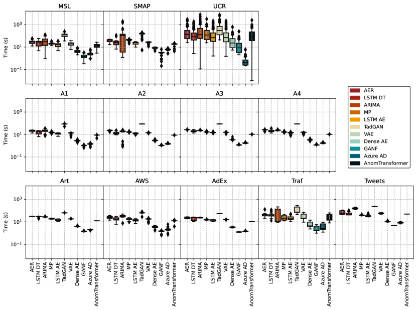
Computational Performance. In addition to quality performance, end-users are interested in pipelines’ computational performance. Figure 5 illustrates how much time (in seconds) on average each pipeline requires for a single signal. Elapsed time includes the time it takes to train a pipeline and time it takes to run inference (detect anomalies). The most time consuming pipeline is TadGAN. It has the highest amount of networks (4 networks) compared to other pipelines. Given the complexity of this model, end-users might want to select an alternative pipeline. Moreover, a user might sacrifice quality performance for computation, or vice versa. Individual end users can make their own decisions about these tradeoffs.

Figure 7: Timeline of pipeline introduction to the benchmark. OrionBench started initially with 2 pipelines; over the course of three years, 7 more pipelines were introduced at different stages.

4.2 Progression of Benchmarks

Stability. As we saw in Figure 4, AER is the highest performing pipeline, was this always the case? OrionBench publishes benchmark results with every package release.

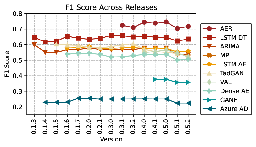
Figure 6 depicts the average F1 Score for each pipeline currently available in our framework. More importantly, if we look closely at Figure 6, we notice three shifts to LSTM DT. First, from version 0.1.3 to 0.1.4, we see a drop in F1 Score due to our change in the overall calculations. Second, from version 0.1.5 to 0.1.6, there is an increase in performance that can be traced back to our hyperparameter setting modifications, where we made them dependent on signal length. Version 0.4.0 shifts our implementation from TensorFlow version 1 to 2 which impacted the underlying implementation. Lastly, in after introducing a new dataset, namely UCR, we notice a drop in the overall performance by pipelines in version 0.5.1 since it was a harder dataset. For Orion developers, running the benchmark every release reassures that no performance disruption has happened. Moreover, it stabilizes pipelines and makes sure that they do not go out of date, especially with dependency package updates.

Pipeline Integration. We expand Figure 6 to showcase exactly when each pipeline was integrated to OrionBench in Figure 7. The first benchmark release version 0.1.3 in September 2020 featured only 2 pipelines. Over time, new models have been developed and integrated. As of today, OrionBench has 9 verified pipelines ranging from classical models to deep learning, made by 5 different contributors. Note that both MP and AnomTransformer are still sandbox pipelines.

4.3 OrionBench in Action

As anomaly detection models continue to be developed, OrionBench allows researchers and end users to understand and compare these models. In this subsection, we walk through two real scenarios where benchmarking was useful for: (1) guiding researchers to develop a new model for unsupervised time series anomaly detection; (2) providing end-users with an existing SOTA model. We show that OrionBench is a commodity benchmarking framework.

Before walking through the aforementioned scenarios, we would like to describe the state of OrionBench. LSTM DT (Hundman et al., 2018) and TadGAN (Geiger et al., 2020) (which was developed by the Orion team) performed competitively against each other until version 0.3.1, when AER (Wong et al., 2022) was introduced. Below, we illustrate the story behind the AER model and how we, the OrionBench developers, were an impartial entity to help benchmark their model.

Scenario 1 – OrionBench guided a researcher to focus in the right direction. Researchers are inspired by the latest innovations in deep learning. They are eager to adopt them for new tasks and explore their capabilities. An independent researcher was keen on introducing attention mechanism to anomaly detection (Vaswani et al., 2017). While the model was promising in local experiments, to assure its performance we decided it to run through the OrionBench. Unfortunately, the model could not do better than both LSTM DT and TadGAN. This reoriented the project direction, and led to the investigation of the successes and limitations of pipelines. Subsequently, it led to development of a deep understanding of where prediction models prevailed compared to reconstruction models and vice versa. OrionBench helped guide this process by cross-referencing model performance with dataset properties. The conclusion was that prediction-based anomaly scores are better at capturing point anomalies than reconstruction-based anomaly scores. Moreover, reconstruction-based anomaly scores are better at capturing longer anomalies. Wong et al. (2022) uncovered more associations related to anomaly scores and error methods. The outcome of this investigation ultimately resulted in a better performing model published as the AER model, which is now the best performing pipeline on OrionBench.

Scenario 2 – OrionBench enabled addition of a latest model and provided an end-user with confidence in other models. We had been working with an end-user from a renowned satellite company for over four years when they approached us with an interest in a new SOTA model. The model was GANF (Dai & Chen, 2022) which has been featured in a news article ⁵⁵5https://news.mit.edu/2022/artificial-intelligence-anomalies-data-0225 that caught their attention. The end-user wanted to know: Should we adopt this model? Several issues can prevent such models from living up to their promised performance in industrial settings. Real-world data are inherently more complex than pristine benchmark datasets. Furthermore, authors often fine-tune their model to the benchmark datasets, neglecting others, causing their model to underperform on unseen datasets. OrionBench, as an independent benchmark, can help determine whether it makes sense to adopt a new model. We integrated GANF to OrionBench. As presented earlier in Figure 4, it was only competitive on the NAB dataset. However, due to the seamless integration of the pipelines, the end-user was still able to apply the pipeline to their own data and obtained valuable results. This emphasizes that the behavior of models differs from one dataset to another, and there is no one-pipeline-fits-all.

5 Conclusion

We present OrionBench – a continuous end-to-end benchmarking framework for unsupervised time series anomaly detection. The benchmark is open-source and publicly available https://github.com/sintel-dev/Orion. As of today, the benchmark holds 24 primitives, 11 pipelines, 12 public datasets, and 2 custom evaluation metrics. We present the qualitative and computational performance of pipelines across all datasets. Moreover, we showcase results our benchmark has accumulated since 2020, highlighting its value for providing continuous evaluations that demonstrate the extensibility and stability of pipelines.

Although the benchmark compares different pipelines, there is no one-pipeline-fits-all datasets. Pipeline selection is still an ambiguous process that highly correlates with the characteristics of the dataset at hand and the type of anomalies present in the dataset. As part of our future work, we would like to focus on the suitability of pipelines and finding the relationship between various attributes of the input and the efficacy of the detection.

References

Aggarwal & Aggarwal (2017) Aggarwal, C. C. and Aggarwal, C. C. An Introduction to Outlier Analysis. Springer, 2017.
Agrawal & Agrawal (2015) Agrawal, S. and Agrawal, J. Survey on anomaly detection using data mining techniques. Procedia Computer Science, 60:708–713, 2015.
Alexandrov et al. (2020) Alexandrov, A., Benidis, K., Bohlke-Schneider, M., Flunkert, V., Gasthaus, J., Januschowski, T., Maddix, D. C., Rangapuram, S., Salinas, D., Schulz, J., Stella, L., Türkmen, A. C., and Wang, Y. GluonTS: Probabilistic and Neural Time Series Modeling in Python. Journal of Machine Learning Research, 21(116):1–6, 2020. URL http://jmlr.org/papers/v21/19-820.html.
Alnegheimish (2022) Alnegheimish, S. Orion – A Machine Learning Framework for Unsupervised Time Series Anomaly Detection. PhD thesis, Massachusetts Institute of Technology, 2022.
Alnegheimish et al. (2022) Alnegheimish, S., Liu, D., Sala, C., Berti-Equille, L., and Veeramachaneni, K. Sintel: A machine learning framework to extract insights from signals. In Proceedings of the 2022 International Conference on Management of Data, SIGMOD ’22, pp. 1855–1865. Association for Computing Machinery, 2022.
Bauer et al. (2021) Bauer, A., Züfle, M., Eismann, S., Grohmann, J., Herbst, N., and Kounev, S. Libra: A benchmark for time series forecasting methods. In Proceedings of the ACM/SPEC International Conference on Performance Engineering, pp. 189–200, 2021.
Bhatnagar et al. (2021) Bhatnagar, A., Kassianik, P., Liu, C., Lan, T., Yang, W., Cassius, R., Sahoo, D., Arpit, D., Subramanian, S., Woo, G., et al. Merlion: A machine learning library for time series. arXiv preprint arXiv:2109.09265, 2021.
Blázquez-García et al. (2021) Blázquez-García, A., Conde, A., Mori, U., and Lozano, J. A. A review on outlier/anomaly detection in time series data. ACM Computing Surveys (CSUR), 54(3):1–33, 2021.
Box & Jenkins (1968) Box, G. E. and Jenkins, G. M. Some recent advances in forecasting and control. Journal of the Royal Statistical Society. Series C (Applied Statistics), 17(2):91–109, 1968.
Campos et al. (2016) Campos, G. O., Zimek, A., Sander, J., Campello, R. J., Micenková, B., Schubert, E., Assent, I., and Houle, M. E. On the evaluation of unsupervised outlier detection: Measures, datasets, and an empirical study. Data Mining and Knowledge Discovery, 30:891–927, 2016.
Chalapathy & Chawla (2019) Chalapathy, R. and Chawla, S. Deep learning for anomaly detection: A survey. arXiv preprint arXiv:1901.03407, 2019.
Chandola et al. (2009) Chandola, V., Banerjee, A., and Kumar, V. Anomaly detection: A survey. ACM computing surveys (CSUR), 41(3):1–58, 2009.
Coleman et al. (2019) Coleman, C., Kang, D., Narayanan, D., Nardi, L., Zhao, T., Zhang, J., Bailis, P., Olukotun, K., Ré, C., and Zaharia, M. Analysis of dawnbench, a time-to-accuracy machine learning performance benchmark. ACM SIGOPS Operating Systems Review, 53(1):14–25, 2019.
Dai & Chen (2022) Dai, E. and Chen, J. Graph-augmented normalizing flows for anomaly detection of multiple time series. 2022. URL https://openreview.net/forum?id=45L_dgP48Vd.
Geiger et al. (2020) Geiger, A., Liu, D., Alnegheimish, S., Cuesta-Infante, A., and Veeramachaneni, K. Tadgan: Time series anomaly detection using generative adversarial networks. In 2020 IEEE International Conference on Big Data (Big Data), pp. 33–43. IEEE, 2020.
Goldstein & Uchida (2016) Goldstein, M. and Uchida, S. A comparative evaluation of unsupervised anomaly detection algorithms for multivariate data. PloS One, 11(4):e0152173, 2016.
Han et al. (2022) Han, S., Hu, X., Huang, H., Jiang, M., and Zhao, Y. Adbench: Anomaly detection benchmark. In Koyejo, S., Mohamed, S., Agarwal, A., Belgrave, D., Cho, K., and Oh, A. (eds.), Advances in Neural Information Processing Systems, volume 35, pp. 32142–32159, 2022.
Hasan et al. (2019) Hasan, M., Islam, M. M., Zarif, M. I. I., and Hashem, M. Attack and anomaly detection in iot sensors in iot sites using machine learning approaches. Internet of Things, 7:100059, 2019.
Hochreiter & Schmidhuber (1997) Hochreiter, S. and Schmidhuber, J. Long short-term memory. Neural computation, 9(8):1735–1780, 1997.
Hundman et al. (2018) Hundman, K., Constantinou, V., Laporte, C., Colwell, I., and Soderstrom, T. Detecting spacecraft anomalies using lstms and nonparametric dynamic thresholding. In Proceedings of the 24th ACM SIGKDD International Conference on Knowledge Discovery & Data Mining, pp. 387–395, 2018.
Jacob et al. (2020) Jacob, V., Song, F., Stiegler, A., Rad, B., Diao, Y., and Tatbul, N. Exathlon: A benchmark for explainable anomaly detection over time series. arXiv preprint arXiv:2010.05073, 2020.
Lai et al. (2021) Lai, K.-H., Zha, D., Xu, J., Zhao, Y., Wang, G., and Hu, X. Revisiting time series outlier detection: Definitions and benchmarks. In Vanschoren, J. and Yeung, S. (eds.), Proceedings of the Neural Information Processing Systems Track on Datasets and Benchmarks, volume 1, 2021.
Lavin & Ahmad (2015) Lavin, A. and Ahmad, S. Evaluating real-time anomaly detection algorithms – the numenta anomaly benchmark. In 2015 IEEE 14th international conference on machine learning and applications (ICMLA), pp. 38–44. IEEE, 2015.
Liu et al. (2015) Liu, D., Zhao, Y., Xu, H., Sun, Y., Pei, D., Luo, J., Jing, X., and Feng, M. Opprentice: Towards practical and automatic anomaly detection through machine learning. In Proceedings of the 2015 internet measurement conference, pp. 211–224, 2015.
Malhotra et al. (2016) Malhotra, P., Ramakrishnan, A., Anand, G., Vig, L., Agarwal, P., and Shroff, G. Lstm-based encoder-decoder for multi-sensor anomaly detection. arXiv preprint arXiv:1607.00148, 2016.
Münz et al. (2007) Münz, G., Li, S., and Carle, G. Traffic anomaly detection using k-means clustering. In Gi/itg workshop mmbnet, volume 7, 2007.
Pang et al. (2021) Pang, G., Shen, C., Cao, L., and Hengel, A. V. D. Deep learning for anomaly detection: A review. ACM Computing Surveys (CSUR), 54(2):1–38, 2021.
Paparrizos et al. (2022) Paparrizos, J., Kang, Y., Boniol, P., Tsay, R. S., Palpanas, T., and Franklin, M. J. Tsb-uad: An end-to-end benchmark suite for univariate time-series anomaly detection. Proceedings of the VLDB Endowment, 15(8):1697–1711, 2022.
Park et al. (2018) Park, D., Hoshi, Y., and Kemp, C. C. A multimodal anomaly detector for robot-assisted feeding using an lstm-based variational autoencoder. IEEE Robotics and Automation Letters, 3(3):1544–1551, 2018.
Patcha & Park (2007) Patcha, A. and Park, J.-M. An overview of anomaly detection techniques: Existing solutions and latest technological trends. Computer Networks, 51(12):3448–3470, 2007.
Pena et al. (2013) Pena, E. H., de Assis, M. V., and Proença, M. L. Anomaly detection using forecasting methods arima and hwds. In 2013 32nd International Conference of the Chilean Computer Science Society (sccc), pp. 63–66. IEEE, 2013.
Ren et al. (2019) Ren, H., Xu, B., Wang, Y., Yi, C., Huang, C., Kou, X., Xing, T., Yang, M., Tong, J., and Zhang, Q. Time-series anomaly detection service at microsoft. In Proceedings of the 25th ACM SIGKDD international conference on knowledge discovery & data mining, pp. 3009–3017, 2019.
Reuther et al. (2018) Reuther, A., Kepner, J., Byun, C., Samsi, S., Arcand, W., Bestor, D., Bergeron, B., Gadepally, V., Houle, M., Hubbell, M., et al. Interactive supercomputing on 40,000 cores for machine learning and data aaalysis. In 2018 IEEE High Performance Extreme Computing Conference (HPEC), pp. 1–6. IEEE, 2018.
Smith et al. (2020) Smith, M. J., Sala, C., Kanter, J. M., and Veeramachaneni, K. The machine learning bazaar: Harnessing the ml ecosystem for effective system development. In Proceedings of the 2020 ACM SIGMOD International Conference on Management of Data, pp. 785–800, 2020.
Syarif et al. (2012) Syarif, I., Prugel-Bennett, A., and Wills, G. Unsupervised clustering approach for network anomaly detection. In Networked Digital Technologies: 4th International Conference, NDT 2012, Dubai, UAE, April 24-26, 2012. Proceedings, Part I 4, pp. 135–145. Springer, 2012.
Taieb et al. (2012) Taieb, S. B., Bontempi, G., Atiya, A. F., and Sorjamaa, A. A review and comparison of strategies for multi-step ahead time series forecasting based on the nn5 forecasting competition. Expert Systems with Applications, 39(8):7067–7083, 2012.
Vaswani et al. (2017) Vaswani, A., Shazeer, N., Parmar, N., Uszkoreit, J., Jones, L., Gomez, A. N., Kaiser, Ł., and Polosukhin, I. Attention is all you need. Advances in Neural Information Processing Systems, 30, 2017.
Wenig et al. (2022) Wenig, P., Schmidl, S., and Papenbrock, T. Timeeval: A benchmarking toolkit for time series anomaly detection algorithms. Proceedings of the VLDB Endowment, 15(12):3678–3681, 2022.
Wong et al. (2022) Wong, L., Liu, D., Berti-Equille, L., Alnegheimish, S., and Veeramachaneni, K. Aer: Auto-encoder with regression for time series anomaly detection. In 2022 IEEE International Conference on Big Data (Big Data), pp. 1152–1161. IEEE, 2022.
Xu et al. (2022) Xu, J., Wu, H., Wang, J., and Long, M. Anomaly transformer: Time series anomaly detection with association discrepancy. In International Conference on Learning Representations, 2022. URL https://openreview.net/forum?id=LzQQ89U1qm_.
Yeh et al. (2016) Yeh, C.-C. M., Zhu, Y., Ulanova, L., Begum, N., Ding, Y., Dau, H. A., Silva, D. F., Mueen, A., and Keogh, E. Matrix profile i: All pairs similarity joins for time series: A unifying view that includes motifs, discords and shapelets. In 2016 IEEE 16th international conference on data mining (ICDM), pp. 1317–1322. IEEE, 2016.

Appendix

Limitations

We acknowledge several limitations of our framework and results. Black box pipelines such as Microsoft’s Azure AD service lack certain levels of transparency. In Figure 6, we noticed that Azure AD improved in version 0.1.7. However, we have no intellect on what has caused this improvement. Unlike other pipelines where we can cross reference change of behaviour to code modification or even updated dependency package releases. Nevertheless, we are still able to monitor the performance of black box pipelines and having some confidence in their stability.

In addition, benchmarks are notorious for requiring massive computing resources, and in this case it is no different. While the models can vary in usage, to perform a comprehensive benchmark, we utilize MIT supercloud (Reuther et al., 2018). When computing resources are limited, on-demand benchmark runs become difficult. We aim to alleviate this challenge with continuous and periodic running benchmarks. Moreover, with every introduction to a new model, a benchmark must be run to add the model to the leaderboard.

Lastly, and most importantly, there is no guarantee that these pipelines will deliver the same performance on real-world datasets. A clear example was demonstrated in Section 4.3 Scenario 2 where GANF produced valuable results for the end-user, however its results in the benchmark are not as promising as some other pipelines. This stresses the importance of pipeline selection based on the characteristics of the datasets and anomalies. Further research is needed to understand the suitability of unsupervised pipelines for a given dataset.

Appendix A Primitives & Pipelines

A.1 Primitive Template

Abstractions in OrionBench of primitives and pipelines are universal representations of end-to-end models, from a signal to a set of detected anomalies. Compared to standard scikit-learn like code, it requires one additional step of creating json files to define these primitives. Figure 8 showcases a template that helps contributors to guides their own primitive.

Once primitives are built, they can be stacked to create a pipeline similar to the example shown in Figure 9. The example shows the json file representation of LSTM DT pipeline.

⬇

{

”name”: ”orion.primitives.primitive.PrimitiveName”,

”contributors”: [”Author <email>”],

”documentation”: ”reference to documentation or paper if available.”,

”description”: ”short description.”,

”classifiers”: {

”type”: ”postprocessor”,

”subtype”: ”anomaly_detector”

”modalities”: [],

”primitive”: ”orion.primitives.primitive.PrimitiveName”,

”fit”: {

”method”: ”fit”,

”args”: [

{

”name”: ”X”,

”type”: ”ndarray”

{

”name”: ”y”,

”type”: ”ndarray”

}

]

”produce”: {

”method”: ”detect”,

”args”: [

{

”name”: ”X”,

”type”: ”ndarray”

{

”name”: ”y”,

”type”: ”ndarray”

}

”output”: [

{

”name”: ”y”,

”type”: ”ndarray”

}

]

”hyperparameters”: {

”fixed”: {

”hyper_name”: {

”type”: ”str”,

”default”: ”value”

}

Figure 8: Primitive template. The first section of the json describes metadata, the second part contains functional information including the names of the methods and their arguments, the third part defines the hyperparameters of the primitive.

⬇

{

”primitives”: [

”mlstars.custom.timeseries_preprocessing.time_segments_aggregate”,

”sklearn.impute.SimpleImputer”,

”sklearn.preprocessing.MinMaxScaler”,

”mlstars.custom.timeseries_preprocessing.rolling_window_sequences”,

”keras.Sequential.LSTMTimeSeriesRegressor”,

”orion.primitives.timeseries_errors.regression_errors”,

”orion.primitives.timeseries_anomalies.find_anomalies”

”init_params”: {

”mlstars.custom.timeseries_preprocessing.time_segments_aggregate#1”: {

”time_column”: ”timestamp”,

”interval”: 21600,

”method”: ”mean”

”sklearn.preprocessing.MinMaxScaler#1”: {

”feature_range”: [

-1,

]

”mlstars.custom.timeseries_preprocessing.rolling_window_sequences#1”: {

”target_column”: 0,

”window_size”: 250

”keras.Sequential.LSTMTimeSeriesRegressor”: {

”epochs”: 35

”orion.primitives.timeseries_anomalies.find_anomalies#1”: {

”window_size_perc”: 30,

”fixed_threshold”: false

}

Figure 9: LSTM DT pipeline example. This is the content present in the json file of the pipeline. The first section defines the stack of primitives used in the pipeline which will be computed to the graph shown previously in Figure 2(a). The init argument initializes some of the hyperparameters for each primitive. This is a detailed version with full primitive names of the hyperparameters shown in Figure 2(c).

A.2 Pipelines

Currently in OrionBench, there are 9 readily available pipelines. They are all unsupervised pipelines. All pipelines and their hyperparameter settings for the benchmark can be explored directly: https://github.com/sintel-dev/Orion/tree/master/orion/pipelines/verified. Below we provide further detail on the mechanisms behind each pipeline.

ARIMA (Pena et al., 2013). ARIMA is an autoregressive integrated moving average model which is a classic statistical analysis model. It is a forecasting model that learns autocorrelations in the time series to predict future values prediction. Since then it has been adapted for anomaly detection. The pipeline computes the prediction error between the original signal and the forecasting one using simple point-wise error. Then it pinpoints where the anomalies are based one when the error exceeds a certain threshold. Particularly, ARIMA pipeline uses a moving window based thresholding technique defined in find_anomalies primitive.

AER (Wong et al., 2022). AER is an autoencoder with regression pipeline. It combines prediction and reconstruction models simultaneously. More specifically, it produces bi-directional predictions (forward & backward) while reconstructing the original time series at the same time by optimizing a joint objective function. The error is then computed as a point-wise error for both forward and backward predictions. As for reconstruction, dynamic time warping is used, which computes the euclidean distance between two time series where one might lag behind another. The total error is then computed as a point-wise product between the three aforementioned errors.

LSTM DT (Hundman et al., 2018). LSTM DT is a prediction-based pipeline using an LSTM model. Similar to ARIMA, it computes the residual between the original signal and predicted one using smoothed point-wise error. Then they apply a non-parametric thresholding method to reduce the amount of false positives.

TadGAN (Geiger et al., 2020). TadGAN is a reconstruction pipeline that uses generative adversarial networks to generate a synthetic time series. To sample a “similar” time series, the model uses an encoder to map the original time series to the latent dimension. There are three possible strategies to compute the errors between the real and synthetic time series. Specifically, point-wise errors, area difference, and dynamic time warping. Most datasets are set to dynamic time warping (dtw) as error.

MP (Yeh et al., 2016). MP is a matrix profile method that seeks to find discords in time series. The pipeline computes the matrix profile of a signal, which essential provides the closes nearest neighbor for each segment. Based on these values, segments with large distance values to their nearest neighbors are anomalous. We use find_anomalies to set the threshold dynamically.

VAE (Park et al., 2018). VAE is a variational autoencoder consisting of an encoder and a decoder with LSTM layers. Similar to previous pipelines, it adopts reconstruction errors to compute the deviation between the original and reconstructed signal.

LSTM AE (Malhotra et al., 2016). LSTM AE is an autoencoder with an LSTM encoder and decoder. This is a simpler variant of VAE. It also uses reconstruction errors to measure the difference between the original and reconstruction signal.

Dense AE. Dense AE is an autoencoder where its properties are exactly similar to that of LSTM AE with the exception of the encoder and decoder layers.

GANF (Dai & Chen, 2022). GANF is density-based methods where they use normalizing flows to learn the distribution of the data with a graph structure to overcome the challenge of high dimensionality. The model outputs an anomaly measure that indicates where the anomalies might be. To convert the output into a list of intervals, we add find_anomalies primitive.

Azure AD (Ren et al., 2019). Azure AD is a black box pipeline which connects to Microsoft’s anomaly detection service ⁶⁶6https://azure.microsoft.com/en-us/products/cognitive-services/anomaly-detector/. To use this pipeline, the user needs to have a subscription to the service. Then the user can update the subscription_key and endpoint in the pipeline json for usage.

AnomTransformer (Xu et al., 2022). AnomTransformer is a transformer based model using a new anomaly-attention mechanism to compute the association discrepancy. The model amplifies the discrepancies between normal and abnormal time points using a minimax strategy. The threshold is set based on the attention values.

Appendix B Data

B.1 Data Format

Time series is a collection of data points that are indexed by time. There are many forms in which time series can be stored, we define a time series as a set of time points, which we represent through integers denoting timestamps, and a corresponding set of values observed at each respective timestamp. Note that no prior pre-processing is required as all pre-processing steps are part of the pipeline, e.g. imputations, scaling, etc.

B.2 Dataset Details

The benchmark currently features 11 publicly accessible datasets from different sources. Table 3 illustrates some of the datasets’ properties. Below, we provide more detailed description for each dataset.

NASA. This dataset is a spacecraft telemetry signals provided by NASA. It was originally released in 2018 as part of the Lstm-DT paper (Hundman et al., 2018) and can be accessed directly from https://github.com/khundman/telemanom. It features two datasets: Mars Science Laboratory (MSL) and Soil Moisture Active Passive (SMAP). MSL contains 27 signals with 36 anomalies. SMAP contains 53 signals with 69 anomalies. In total, NASA datasets has 80 signals with 105 anomalies. This dataset was pre-split into training and testing partitions. In our benchmark, we train the pipeline using the training data, and apply detection to only the testing data.

NAB. Part of the Numenta benchmark (Lavin & Ahmad, 2015) is the NAB dataset https://github.com/numenta/NAB. This datasets includes multiple types of time series data from various applications and domains In our benchmark we selected five sub-datasets (name: # signals, # anomalies): artWithAnomaly (Art: 6, 6): this dataset was artificially generated; realAWSCloudwatch (AWS: 17, 20): this dataset contains AWS server metrics collected by AmazonCloudwatch service such as CPU Utilization; realAdExchange (AdEx: 5, 11), this dataset contains online advertisement clicking rate metrics such as cost-per-click; realTraffic (Traf: 7, 14): this dataset contains real time traffic metrics from the Twin Cities Metro area in Minnesota such as occupancy, speed, etc; and realTweets (Tweets: 10, 33): this dataset contains metrics of a collection of Twitter mentions of companies (e.g. Google) such as number of mentions each 5 minutes.

Yahoo S5. This dataset contains four different sub-datasets. A1 dataset is based on real production traffic of Yahoo computing systems with 67 signals and 179 anomalies. On the other hand, A2, A3 and A4 are all synthetic datasets with 100 signals each and 200, 939, and 835 anomalies respectively. There are many anomalies in this dataset with over 2,153 in 367 signals, averaging 5.8 anomalies in each signal. Most of the anomalies in A3 and A4 are short and last for only a few points in time. Data can be requested from Yahoo’s website https://webscope.sandbox.yahoo.com/catalog.php?datatype=s&did=70. In our benchmark, we train and apply detection to the same entire signal.

UCR. This dataset was released in a SIGKDD competition in 2021 https://www.cs.ucr.edu/~eamonn/time_series_data_2018/UCR_TimeSeriesAnomalyDatasets2021.zip. It contains 250 signals with only one anomaly in each signal. The anomalies themselves were artificially introduced to the signal. More specifically, in many times they are synthetic anomalies, or a consequence of flipping/smoothing/interpolating/reversing/prolonging normal segments to create anomalies. The dataset was created to have more challenging cases of anomalies.

Appendix C Evaluation

This section provides further details on our evaluation setup and obtained results. Code to reproduce Figures and Tables are provided https://github.com/sarahmish/orionbench-paper

C.1 Evaluation Setup

Results presented in Section 4 are reported based on version 0.5.0 of Orion which is also released on pip ⁷⁷7https://pypi.org/project/orion-ml/0.5.0/. We recommend setting up a new python environment before installing Orion. Currently the library is supported in python 3.6, 3.7, and 3.8.

Evaluation Strategy. Measuring the performance of unsupervised time series anomaly detection pipelines is more nuanced than the usual classification metrics. OrionBench compares detected anomalies with ground truth labels according to well-defined metrics. This can be done using either weighted segment or overlapping segment (Alnegheimish et al., 2022). For our evaluation in this paper, we use overlapping segment exclusively. Using overlapping segment, for each experiment run (which is an evaluation of one pipeline on one signal), we record the number of true positives (TP), false positive (FP), and false negative (FN) obtained. Because anomalies are scarce and in many signals only one anomaly exists (or none), in many cases precision and recall scores will be undefined on a signal level. Therefore, we compute the scores on a dataset level.

precision=\frac{\sum_{s\in\mathcal{S}}TP_{s}}{\sum_{s\in\mathcal{S}}TP_{s}+FP_{s}}\qquad recall=\frac{\sum_{s\in\mathcal{S}}TP_{s}}{\sum_{s\in\mathcal{S}}TP_{s}+FN_{s}}

For a given dataset with a set of signals $\mathcal{S}$ , we compute the total true positives, false positives, and false negatives within every signal in that set. Then we compute the score for each pipeline according to the metric of interest whether it is precision, recall, or f1 score. The computation of f1 score is standard from precision and recall ( $f1=2\times\frac{precision\times recall}{precision+recall}$ ).

Recorded Information. During the benchmark process, information regarding performance, computation, diagnostics, etc. gets recorded. Below we list all the information we store for each experiment. An experiment is defined as a single pipeline trained on a single time series then used for detection for the same time series.

•

dataset: the dataset that the signal belongs to, e.g. SMAP.
•

pipeline: the name of the pipeline, e.g. AER.
•

signal: the name of the signal, e.g. S-1.
•

iteration: each experiment can be run for $k$ iterations.
•

f1, precision, recall: the evaluated metrics, in many cases it is undefined.
•

tn, fp, fn, tp: the evaluated number of true negatives, false positives, false negatives, true positives respectively. In overlapping segment approach, tn does not have a value given the nature of evaluation.
•

status: whether or not the experiment ran from beginning to end without issue.
•

elapsed: how much runtime each experiment took (includes training and inference).
•

run_id: the process identification number.

The benchmark results are saved as .csv files and stored directly in the Github repositories: https://github.com/sintel-dev/Orion/tree/master/benchmark/results. Moreover, the pipelines used in each experiment are saved for reproduciblity measures. Due to their large size, we store these pipelines on a local server. However, part of our endeavour is to make these pipelines public as well such that they can be used and inspected.

C.2 Benchmark Results

Figure 10 illustrates the F1 score obtained per dataset. Observing the average values per dataset, AER seems to score the highest on most datasets. However, other pipelines such as LSTM DT are comparable or outperform AER in certain cases. Each pipeline has its strengths and the performance varies from one dataset to another.

Pipeline scalability is an important aspect to address for many end-users. The reported wall time of each pipeline per dataset is shown in Figure 11. TadGAN takes minutes to run while other pipelines seem to finish in several seconds. The fastest pipelines are GANF and Azure AD. Azure AD is an inference only pipeline, and GANF is fast to train.

Table 4: Leaderboard showing the number of wins of a particular pipeline compared with classic pipeline ARIMA in terms of F1 Score on 12 datasets.

Pipeline	ARIMA (Box & Jenkins, 1968)
	Outperform
AER, 2022 (Wong et al., 2022)	12
TadGAN, 2020 (Geiger et al., 2020)	7
LSTM DT, 2018 (Hundman et al., 2018)	8
LSTM AE, 2016 (Malhotra et al., 2016)	8
VAE, 2018 (Park et al., 2018)	8
GANF, 2022 (Dai & Chen, 2022)	7
MP, 2016 (Yeh et al., 2016)	6
Azure AD, 2019 (Ren et al., 2019)	0

C.3 Leaderboard

With every release, we present a leaderboard similar to Table 4. It depicts the number of times each pipeline outperformed ARIMA in F1 Score (maximum # datasets). Specifically, Table 4 is generated from benchmark version 0.5.2. It provides an overall view of how deep learning models perform compared to a classical method such as ARIMA. AER fluctuates between 11 and 12, beating ARIMA on almost every dataset, with the exception of AdEx dataset.

C.4 Computational Cost Across Releases

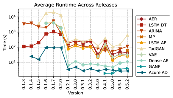
In addition to quality stability shown in Figure 6, we can monitor the runtime execution of the benchmark. We illustrate the average runtime for each pipeline across 15 releases in Figure 12. There is a clear improvement in average runtime in release 0.2.1. This increase in speed traces back to an internal change of the API’s code. More specifically, pipelines builds were adjusted to only build once to reduce overhead during the fit and detect process. Looking back at the development plan, this is reflected in Issue #261 where we see exact alterations made to the code.

Moreover, in version 0.4.0, the package migrated to TensorFlow 2.0 which consequently made the pipelines faster in GPU mode. However, in version 0.4.1 the pipelines were executed without GPU, which is evident by the slight increase in runtime.

C.5 Qualitative Performance Across Releases

The detailed sheets of benchmark runs are stored directly in the repository: https://github.com/sintel-dev/Orion/tree/master/benchmark/results. The following tables report the F1 score, precision, and recall metrics for each pipeline across all releases as of today.

•

version 0.5.2, pipelines 10, datasets 12, release date: October 19^th 2023.
•

version 0.5.1, pipelines 9, datasets 12, release date: August 16^th 2023.
•

version 0.5.0, pipelines 9, datasets 11, release date: May 23^rd 2023.
•

version 0.4.1, pipelines 9, datasets 11, release date: January 31^st 2023.
•

version 0.4.0, pipelines 8, datasets 11, release date: November 10^th 2022.
•

version 0.3.2, pipelines 7, datasets 11, release date: July 4^th 2022.
•

version 0.3.1, pipelines 7, datasets 11, release date: April 26^th 2022.
•

version 0.3.0, pipelines 6, datasets 11, release date: March 31^st 2022.
•

version 0.2.1, pipelines 6, datasets 11, release date: February 18^th 2022.
•

version 0.2.0, pipelines 6, datasets 11, release date: October 11^th 2021.
•

version 0.1.7, pipelines 6, datasets 11, release date: May 4^th 2021.
•

version 0.1.6, pipelines 6, datasets 11, release date: March 8^th 2021.
•

version 0.1.5, pipelines 4, datasets 11, release date: December 25^th 2020.
•

version 0.1.4, pipelines 3, datasets 11, release date: October 16^th 2020.
•

version 0.1.3, pipelines 2, datasets 11, release date: September 29^th 2020.

Table 5: Benchmark Results

	NASA		UCR	Yahoo S5				NAB
Pipeline	MSL	SMAP	UCR	A1	A2	A3	A4	Art	AWS	AdEx	Traf	Tweets
F1 Score
AER	0.605 $\pm$ 0.02	0.792 $\pm$ 0.02	0.474 $\pm$ 0.01	0.784 $\pm$ 0.01	0.984 $\pm$ 0.00	0.889 $\pm$ 0.01	0.712 $\pm$ 0.01	0.682 $\pm$ 0.16	0.737 $\pm$ 0.02	0.708 $\pm$ 0.04	0.691 $\pm$ 0.03	0.565 $\pm$ 0.02
LSTM DT	0.483 $\pm$ 0.01	0.713 $\pm$ 0.02	0.399 $\pm$ 0.01	0.736 $\pm$ 0.02	0.978 $\pm$ 0.00	0.738 $\pm$ 0.01	0.649 $\pm$ 0.01	0.404 $\pm$ 0.03	0.495 $\pm$ 0.03	0.734 $\pm$ 0.02	0.634 $\pm$ 0.04	0.556 $\pm$ 0.01
ARIMA	0.435 $\pm$ 0.00	0.324 $\pm$ 0.00	0.090 $\pm$ 0.00	0.744 $\pm$ 0.00	0.816 $\pm$ 0.00	0.782 $\pm$ 0.00	0.684 $\pm$ 0.00	0.429 $\pm$ 0.00	0.472 $\pm$ 0.00	0.727 $\pm$ 0.00	0.429 $\pm$ 0.00	0.513 $\pm$ 0.00
MP	0.474 $\pm$ 0.00	0.423 $\pm$ 0.00	0.072 $\pm$ 0.00	0.507 $\pm$ 0.00	0.897 $\pm$ 0.00	0.793 $\pm$ 0.00	0.825 $\pm$ 0.00	0.571 $\pm$ 0.00	0.440 $\pm$ 0.00	0.692 $\pm$ 0.00	0.310 $\pm$ 0.00	0.343 $\pm$ 0.00
LSTM AE	0.493 $\pm$ 0.05	0.672 $\pm$ 0.03	0.315 $\pm$ 0.01	0.595 $\pm$ 0.01	0.871 $\pm$ 0.02	0.444 $\pm$ 0.01	0.238 $\pm$ 0.01	0.594 $\pm$ 0.07	0.754 $\pm$ 0.02	0.665 $\pm$ 0.06	0.490 $\pm$ 0.02	0.513 $\pm$ 0.02
TadGAN	0.576 $\pm$ 0.02	0.601 $\pm$ 0.02	0.173 $\pm$ 0.01	0.564 $\pm$ 0.02	0.817 $\pm$ 0.01	0.413 $\pm$ 0.02	0.342 $\pm$ 0.02	0.577 $\pm$ 0.08	0.627 $\pm$ 0.03	0.716 $\pm$ 0.04	0.527 $\pm$ 0.05	0.528 $\pm$ 0.04
VAE	0.492 $\pm$ 0.02	0.649 $\pm$ 0.01	0.345 $\pm$ 0.01	0.595 $\pm$ 0.01	0.817 $\pm$ 0.01	0.433 $\pm$ 0.02	0.247 $\pm$ 0.02	0.646 $\pm$ 0.03	0.710 $\pm$ 0.01	0.554 $\pm$ 0.05	0.524 $\pm$ 0.03	0.536 $\pm$ 0.02
Dense AE	0.524 $\pm$ 0.02	0.680 $\pm$ 0.02	0.206 $\pm$ 0.01	0.649 $\pm$ 0.01	0.894 $\pm$ 0.01	0.077 $\pm$ 0.00	0.093 $\pm$ 0.01	0.545 $\pm$ 0.00	0.756 $\pm$ 0.02	0.595 $\pm$ 0.02	0.523 $\pm$ 0.04	0.512 $\pm$ 0.02
GANF	0.438 $\pm$ 0.02	0.463 $\pm$ 0.00	0.144 $\pm$ 0.00	0.095 $\pm$ 0.01	0.156 $\pm$ 0.01	0.008 $\pm$ 0.00	0.150 $\pm$ 0.00	0.667 $\pm$ 0.00	0.578 $\pm$ 0.00	0.308 $\pm$ 0.00	0.556 $\pm$ 0.02	0.673 $\pm$ 0.01
Azure AD	0.051 $\pm$ 0.00	0.019 $\pm$ 0.00	0.015 $\pm$ 0.00	0.280 $\pm$ 0.00	0.653 $\pm$ 0.00	0.702 $\pm$ 0.00	0.344 $\pm$ 0.00	0.054 $\pm$ 0.00	0.112 $\pm$ 0.00	0.228 $\pm$ 0.04	0.112 $\pm$ 0.00	0.186 $\pm$ 0.01
AnomTransformer	0.431 $\pm$ 0.03	0.283 $\pm$ 0.02	0.017 $\pm$ 0.00	0.555 $\pm$ 0.01	0.613 $\pm$ 0.02	0.779 $\pm$ 0.01	0.577 $\pm$ 0.01	0.384 $\pm$ 0.10	0.456 $\pm$ 0.03	0.501 $\pm$ 0.04	0.365 $\pm$ 0.03	0.315 $\pm$ 0.01
Precision
AER	0.601 $\pm$ 0.05	0.832 $\pm$ 0.02	0.391 $\pm$ 0.01	0.809 $\pm$ 0.02	0.983 $\pm$ 0.01	0.992 $\pm$ 0.00	0.927 $\pm$ 0.01	0.602 $\pm$ 0.13	0.804 $\pm$ 0.04	0.566 $\pm$ 0.04	0.562 $\pm$ 0.02	0.572 $\pm$ 0.03
LSTM DT	0.370 $\pm$ 0.01	0.655 $\pm$ 0.02	0.338 $\pm$ 0.01	0.690 $\pm$ 0.02	0.972 $\pm$ 0.01	0.988 $\pm$ 0.01	0.902 $\pm$ 0.01	0.327 $\pm$ 0.01	0.417 $\pm$ 0.05	0.580 $\pm$ 0.02	0.491 $\pm$ 0.04	0.514 $\pm$ 0.02
ARIMA	0.455 $\pm$ 0.00	0.307 $\pm$ 0.00	0.102 $\pm$ 0.00	0.684 $\pm$ 0.00	0.772 $\pm$ 0.00	0.998 $\pm$ 0.00	0.955 $\pm$ 0.00	0.375 $\pm$ 0.00	0.405 $\pm$ 0.00	0.727 $\pm$ 0.00	0.429 $\pm$ 0.00	0.444 $\pm$ 0.00
MP	0.346 $\pm$ 0.00	0.291 $\pm$ 0.00	0.039 $\pm$ 0.00	0.448 $\pm$ 0.00	0.824 $\pm$ 0.00	0.952 $\pm$ 0.00	0.946 $\pm$ 0.00	0.500 $\pm$ 0.00	0.314 $\pm$ 0.00	0.600 $\pm$ 0.00	0.205 $\pm$ 0.00	0.324 $\pm$ 0.00
LSTM AE	0.489 $\pm$ 0.07	0.638 $\pm$ 0.04	0.229 $\pm$ 0.01	0.625 $\pm$ 0.00	0.835 $\pm$ 0.04	0.944 $\pm$ 0.01	0.672 $\pm$ 0.01	0.627 $\pm$ 0.04	0.827 $\pm$ 0.04	0.602 $\pm$ 0.04	0.447 $\pm$ 0.01	0.571 $\pm$ 0.03
TadGAN	0.493 $\pm$ 0.02	0.531 $\pm$ 0.03	0.125 $\pm$ 0.01	0.636 $\pm$ 0.02	0.809 $\pm$ 0.01	0.739 $\pm$ 0.03	0.586 $\pm$ 0.02	0.485 $\pm$ 0.07	0.604 $\pm$ 0.05	0.707 $\pm$ 0.07	0.429 $\pm$ 0.04	0.559 $\pm$ 0.05
VAE	0.466 $\pm$ 0.02	0.595 $\pm$ 0.01	0.263 $\pm$ 0.01	0.584 $\pm$ 0.01	0.727 $\pm$ 0.02	0.842 $\pm$ 0.01	0.653 $\pm$ 0.03	0.629 $\pm$ 0.05	0.720 $\pm$ 0.02	0.484 $\pm$ 0.06	0.508 $\pm$ 0.04	0.608 $\pm$ 0.02
Dense AE	0.573 $\pm$ 0.02	0.724 $\pm$ 0.02	0.177 $\pm$ 0.01	0.726 $\pm$ 0.01	0.954 $\pm$ 0.01	0.964 $\pm$ 0.01	0.553 $\pm$ 0.01	0.600 $\pm$ 0.00	0.832 $\pm$ 0.02	0.657 $\pm$ 0.06	0.483 $\pm$ 0.04	0.586 $\pm$ 0.01
GANF	0.712 $\pm$ 0.03	0.786 $\pm$ 0.00	0.107 $\pm$ 0.00	0.286 $\pm$ 0.00	0.282 $\pm$ 0.02	1.000 $\pm$ 0.00	0.977 $\pm$ 0.01	1.000 $\pm$ 0.00	0.867 $\pm$ 0.00	1.000 $\pm$ 0.00	0.630 $\pm$ 0.06	0.650 $\pm$ 0.01
Azure AD	0.026 $\pm$ 0.00	0.009 $\pm$ 0.00	0.008 $\pm$ 0.00	0.167 $\pm$ 0.00	0.484 $\pm$ 0.00	0.542 $\pm$ 0.00	0.217 $\pm$ 0.00	0.028 $\pm$ 0.00	0.060 $\pm$ 0.00	0.131 $\pm$ 0.02	0.059 $\pm$ 0.00	0.105 $\pm$ 0.00
AnomTransformer	0.282 $\pm$ 0.03	0.170 $\pm$ 0.01	0.009 $\pm$ 0.00	0.497 $\pm$ 0.01	0.494 $\pm$ 0.03	0.850 $\pm$ 0.01	0.758 $\pm$ 0.01	0.253 $\pm$ 0.10	0.325 $\pm$ 0.02	0.352 $\pm$ 0.03	0.229 $\pm$ 0.02	0.188 $\pm$ 0.01
Recall
AER	0.611 $\pm$ 0.02	0.755 $\pm$ 0.01	0.602 $\pm$ 0.01	0.761 $\pm$ 0.01	0.985 $\pm$ 0.00	0.805 $\pm$ 0.01	0.578 $\pm$ 0.01	0.800 $\pm$ 0.22	0.680 $\pm$ 0.02	0.945 $\pm$ 0.05	0.900 $\pm$ 0.08	0.558 $\pm$ 0.02
LSTM DT	0.694 $\pm$ 0.02	0.782 $\pm$ 0.02	0.488 $\pm$ 0.01	0.788 $\pm$ 0.02	0.984 $\pm$ 0.00	0.590 $\pm$ 0.01	0.507 $\pm$ 0.01	0.533 $\pm$ 0.07	0.613 $\pm$ 0.02	1.000 $\pm$ 0.00	0.900 $\pm$ 0.04	0.606 $\pm$ 0.02
ARIMA	0.417 $\pm$ 0.00	0.343 $\pm$ 0.00	0.080 $\pm$ 0.00	0.815 $\pm$ 0.00	0.865 $\pm$ 0.00	0.643 $\pm$ 0.00	0.533 $\pm$ 0.00	0.500 $\pm$ 0.00	0.567 $\pm$ 0.00	0.727 $\pm$ 0.00	0.429 $\pm$ 0.00	0.606 $\pm$ 0.00
MP	0.750 $\pm$ 0.00	0.776 $\pm$ 0.00	0.427 $\pm$ 0.00	0.584 $\pm$ 0.00	0.985 $\pm$ 0.00	0.679 $\pm$ 0.00	0.732 $\pm$ 0.00	0.667 $\pm$ 0.00	0.733 $\pm$ 0.00	0.818 $\pm$ 0.00	0.643 $\pm$ 0.00	0.364 $\pm$ 0.00
LSTM AE	0.500 $\pm$ 0.04	0.710 $\pm$ 0.01	0.506 $\pm$ 0.00	0.569 $\pm$ 0.01	0.912 $\pm$ 0.01	0.290 $\pm$ 0.01	0.145 $\pm$ 0.01	0.567 $\pm$ 0.09	0.693 $\pm$ 0.01	0.745 $\pm$ 0.10	0.543 $\pm$ 0.04	0.467 $\pm$ 0.02
TadGAN	0.694 $\pm$ 0.05	0.696 $\pm$ 0.04	0.282 $\pm$ 0.02	0.507 $\pm$ 0.02	0.824 $\pm$ 0.01	0.287 $\pm$ 0.01	0.242 $\pm$ 0.01	0.733 $\pm$ 0.15	0.653 $\pm$ 0.04	0.727 $\pm$ 0.00	0.686 $\pm$ 0.08	0.503 $\pm$ 0.06
VAE	0.522 $\pm$ 0.02	0.713 $\pm$ 0.02	0.501 $\pm$ 0.02	0.608 $\pm$ 0.02	0.933 $\pm$ 0.01	0.291 $\pm$ 0.01	0.152 $\pm$ 0.02	0.667 $\pm$ 0.00	0.700 $\pm$ 0.00	0.655 $\pm$ 0.08	0.543 $\pm$ 0.04	0.479 $\pm$ 0.01
Dense AE	0.483 $\pm$ 0.02	0.642 $\pm$ 0.02	0.247 $\pm$ 0.01	0.587 $\pm$ 0.01	0.841 $\pm$ 0.01	0.040 $\pm$ 0.00	0.051 $\pm$ 0.00	0.500 $\pm$ 0.00	0.693 $\pm$ 0.03	0.545 $\pm$ 0.00	0.571 $\pm$ 0.05	0.455 $\pm$ 0.02
GANF	0.317 $\pm$ 0.02	0.328 $\pm$ 0.00	0.223 $\pm$ 0.00	0.057 $\pm$ 0.01	0.108 $\pm$ 0.01	0.002 $\pm$ 0.00	0.081 $\pm$ 0.00	0.500 $\pm$ 0.00	0.433 $\pm$ 0.00	0.182 $\pm$ 0.00	0.500 $\pm$ 0.00	0.697 $\pm$ 0.00
Azure AD	0.806 $\pm$ 0.00	0.940 $\pm$ 0.00	0.176 $\pm$ 0.00	0.848 $\pm$ 0.00	1.000 $\pm$ 0.00	0.998 $\pm$ 0.00	0.837 $\pm$ 0.00	1.000 $\pm$ 0.00	0.833 $\pm$ 0.00	0.909 $\pm$ 0.00	1.000 $\pm$ 0.00	0.818 $\pm$ 0.00
AnomTransformer	0.928 $\pm$ 0.03	0.854 $\pm$ 0.02	0.658 $\pm$ 0.04	0.628 $\pm$ 0.02	0.809 $\pm$ 0.02	0.718 $\pm$ 0.02	0.465 $\pm$ 0.02	0.867 $\pm$ 0.07	0.767 $\pm$ 0.04	0.873 $\pm$ 0.05	0.914 $\pm$ 0.03	0.958 $\pm$ 0.05

Table 6: Benchmark Summary Results Version 0.5.1

	NASA		UCR	Yahoo S5				NAB
Pipeline	MSL	SMAP	UCR	A1	A2	A3	A4	Art	AWS	AdEx	Traf	Tweets
F1 Score
AER	0.587	0.775	0.474	0.780	0.987	0.869	0.686	0.769	0.750	0.733	0.611	0.581
LSTM DT	0.485	0.707	0.417	0.724	0.987	0.744	0.644	0.400	0.494	0.759	0.667	0.600
ARIMA	0.435	0.326	0.090	0.744	0.816	0.782	0.684	0.429	0.472	0.727	0.429	0.513
MP	0.474	0.423	0.051	0.507	0.897	0.793	0.825	0.571	0.440	0.692	0.305	0.343
LSTM AE	0.479	0.662	0.332	0.619	0.874	0.460	0.227	0.667	0.750	0.615	0.471	0.533
TadGAN	0.568	0.590	0.173	0.552	0.806	0.408	0.321	0.571	0.603	0.583	0.529	0.606
VAE	0.486	0.649	0.339	0.556	0.817	0.415	0.236	0.462	0.737	0.538	0.483	0.533
Dense AE	0.537	0.641	0.202	0.640	0.885	0.078	0.102	0.545	0.800	0.632	0.500	0.508
GANF	0.462	0.463	0.147	0.086	0.171	0.008	0.152	0.667	0.578	0.308	0.583	0.667
Azure AD	0.051	0.019	0.015	0.280	0.653	0.702	0.344	0.056	0.112	0.163	0.117	0.176
Precision
AER	0.564	0.806	0.385	0.816	0.990	0.992	0.920	0.714	0.808	0.579	0.500	0.621
LSTM DT	0.373	0.650	0.352	0.680	0.990	0.988	0.892	0.333	0.404	0.611	0.545	0.568
ARIMA	0.455	0.311	0.102	0.684	0.772	0.998	0.955	0.375	0.405	0.727	0.429	0.444
MP	0.346	0.291	0.027	0.448	0.824	0.952	0.946	0.500	0.314	0.600	0.200	0.324
LSTM AE	0.486	0.639	0.245	0.652	0.833	0.932	0.675	0.667	0.808	0.533	0.400	0.593
TadGAN	0.511	0.517	0.125	0.624	0.758	0.736	0.532	0.500	0.576	0.538	0.450	0.606
VAE	0.474	0.583	0.259	0.540	0.723	0.857	0.619	0.429	0.778	0.467	0.467	0.593
Dense AE	0.581	0.672	0.172	0.715	0.949	0.974	0.566	0.600	0.880	0.750	0.500	0.577
GANF	0.750	0.786	0.111	0.281	0.300	1.000	0.986	1.000	0.867	1.000	0.700	0.639
Azure AD	0.026	0.009	0.008	0.167	0.484	0.542	0.217	0.029	0.060	0.089	0.062	0.099
Recall
AER	0.611	0.746	0.616	0.747	0.985	0.773	0.547	0.833	0.700	1.000	0.786	0.545
LSTM DT	0.694	0.776	0.512	0.775	0.985	0.596	0.504	0.500	0.633	1.000	0.857	0.636
ARIMA	0.417	0.343	0.080	0.815	0.865	0.643	0.533	0.500	0.567	0.727	0.429	0.606
MP	0.750	0.776	0.432	0.584	0.985	0.679	0.732	0.667	0.733	0.818	0.643	0.364
LSTM AE	0.472	0.687	0.512	0.590	0.920	0.306	0.137	0.667	0.700	0.727	0.571	0.485
TadGAN	0.639	0.687	0.280	0.494	0.860	0.282	0.230	0.667	0.633	0.636	0.643	0.606
VAE	0.500	0.731	0.492	0.573	0.940	0.274	0.146	0.500	0.700	0.636	0.500	0.485
Dense AE	0.500	0.612	0.244	0.579	0.830	0.040	0.056	0.500	0.733	0.545	0.500	0.455
GANF	0.333	0.328	0.220	0.051	0.120	0.004	0.083	0.500	0.433	0.182	0.500	0.697
Azure AD	0.806	0.940	0.176	0.848	1.000	0.998	0.837	1.000	0.833	0.909	1.000	0.818

Table 7: Benchmark Summary Results Version 0.5.2

	NASA		UCR	Yahoo S5				NAB
Pipeline	MSL	SMAP	UCR	A1	A2	A3	A4	Art	AWS	AdEx	Traf	Tweets
F1 Score
AER	0.575	0.803	0.482	0.799	0.987	0.898	0.712	0.500	0.750	0.667	0.703	0.571
LSTM DT	0.471	0.730	0.393	0.743	0.980	0.734	0.639	0.400	0.494	0.710	0.632	0.560
ARIMA	0.435	0.326	0.090	0.744	0.816	0.782	0.684	0.429	0.472	0.727	0.429	0.513
LSTM AE	0.533	0.658	0.311	0.593	0.852	0.452	0.252	0.545	0.737	0.667	0.500	0.542
TadGAN	0.571	0.592	0.172	0.547	0.809	0.427	0.324	0.667	0.645	0.727	0.486	0.552
VAE	0.475	0.653	0.340	0.599	0.806	0.424	0.227	0.667	0.700	0.609	0.516	0.542
Dense AE	0.500	0.692	0.199	0.656	0.902	0.080	0.094	0.545	0.764	0.600	0.467	0.508
GANF	0.462	0.463	0.147	0.086	0.171	0.008	0.152	0.667	0.578	0.308	0.583	0.667
Azure AD	0.051	0.019	0.015	0.280	0.653	0.702	0.344	0.056	0.112	0.163	0.117	0.176
Precision
AER	0.568	0.850	0.402	0.830	0.99	0.995	0.931	0.500	0.808	0.526	0.565	0.600
LSTM DT	0.364	0.667	0.332	0.696	0.975	0.979	0.898	0.333	0.404	0.550	0.500	0.500
ARIMA	0.455	0.311	0.102	0.684	0.772	0.998	0.955	0.375	0.405	0.727	0.429	0.444
LSTM AE	0.513	0.608	0.224	0.629	0.802	0.946	0.690	0.600	0.778	0.615	0.444	0.615
TadGAN	0.473	0.529	0.124	0.621	0.803	0.736	0.569	0.556	0.625	0.727	0.391	0.640
VAE	0.432	0.600	0.256	0.582	0.714	0.834	0.639	0.667	0.700	0.583	0.471	0.615
Dense AE	0.571	0.714	0.166	0.739	0.955	0.975	0.558	0.600	0.840	0.667	0.438	0.577
GANF	0.750	0.786	0.111	0.281	0.300	1.000	0.986	1.000	0.867	1.000	0.700	0.639
Azure AD	0.026	0.009	0.008	0.167	0.484	0.542	0.217	0.029	0.060	0.089	0.062	0.099
Recall
AER	0.583	0.761	0.604	0.770	0.985	0.818	0.577	0.500	0.700	0.909	0.929	0.545
LSTM DT	0.667	0.806	0.484	0.798	0.985	0.587	0.496	0.500	0.633	1.000	0.857	0.636
ARIMA	0.417	0.343	0.080	0.815	0.865	0.643	0.533	0.500	0.567	0.727	0.429	0.606
LSTM AE	0.556	0.716	0.508	0.562	0.910	0.297	0.154	0.500	0.700	0.727	0.571	0.485
TadGAN	0.722	0.672	0.280	0.489	0.815	0.300	0.226	0.833	0.667	0.727	0.643	0.485
VAE	0.528	0.716	0.504	0.618	0.925	0.284	0.138	0.667	0.700	0.636	0.571	0.485
Dense AE	0.444	0.672	0.248	0.590	0.855	0.042	0.051	0.500	0.700	0.545	0.500	0.455
GANF	0.333	0.328	0.220	0.051	0.120	0.004	0.083	0.500	0.433	0.182	0.500	0.697
Azure AD	0.806	0.94	0.176	0.848	1.000	0.998	0.837	1.000	0.833	0.909	1.000	0.818

Table 8: Benchmark Summary Results Version 0.5.0

	NASA		Yahoo S5				NAB
Pipeline	MSL	SMAP	A1	A2	A3	A4	Art	AWS	AdEx	Traf	Tweets
F1 Score
AER	0.632	0.784	0.767	0.978	0.878	0.708	0.769	0.727	0.667	0.686	0.603
LSTM DT	0.481	0.708	0.726	0.973	0.740	0.638	0.400	0.474	0.759	0.649	0.560
ARIMA	0.435	0.324	0.744	0.816	0.782	0.684	0.429	0.472	0.727	0.429	0.513
LSTM AE	0.514	0.686	0.600	0.888	0.443	0.227	0.667	0.800	0.522	0.500	0.483
TadGAN	0.482	0.573	0.612	0.818	0.371	0.327	0.615	0.645	0.538	0.512	0.551
VAE	0.538	0.635	0.556	0.803	0.457	0.257	0.545	0.700	0.593	0.571	0.567
Dense AE	0.545	0.683	0.629	0.877	0.087	0.098	0.545	0.741	0.632	0.571	0.500
GANF	0.462	0.463	0.086	0.171	0.008	0.152	0.667	0.578	0.308	0.583	0.667
Azure AD	0.051	0.019	0.280	0.653	0.702	0.344	0.054	0.112	0.244	0.111	0.189
Precision
AER	0.600	0.845	0.795	0.970	0.991	0.923	0.714	0.800	0.526	0.571	0.633
LSTM DT	0.368	0.662	0.678	0.961	0.989	0.883	0.333	0.391	0.611	0.522	0.500
ARIMA	0.455	0.307	0.684	0.772	0.998	0.955	0.375	0.405	0.727	0.429	0.444
LSTM AE	0.529	0.658	0.630	0.846	0.929	0.679	0.667	0.880	0.500	0.444	0.560
TadGAN	0.426	0.539	0.690	0.806	0.703	0.558	0.571	0.625	0.467	0.379	0.528
VAE	0.500	0.580	0.549	0.703	0.869	0.680	0.600	0.700	0.500	0.571	0.630
Dense AE	0.600	0.729	0.723	0.964	0.977	0.549	0.600	0.833	0.750	0.571	0.609
GANF	0.750	0.786	0.281	0.300	1.000	0.986	1.000	0.867	1.000	0.700	0.639
Azure AD	0.026	0.009	0.167	0.484	0.542	0.217	0.028	0.060	0.141	0.059	0.107
Recall
AER	0.667	0.731	0.742	0.985	0.789	0.575	0.833	0.667	0.909	0.857	0.576
LSTM DT	0.694	0.761	0.781	0.985	0.591	0.499	0.500	0.600	1.000	0.857	0.636
ARIMA	0.417	0.343	0.815	0.865	0.643	0.533	0.500	0.567	0.727	0.429	0.606
LSTM AE	0.500	0.716	0.573	0.935	0.291	0.137	0.667	0.733	0.545	0.571	0.424
TadGAN	0.556	0.612	0.551	0.830	0.252	0.231	0.667	0.667	0.636	0.786	0.576
VAE	0.583	0.701	0.562	0.935	0.310	0.158	0.500	0.700	0.727	0.571	0.515
Dense AE	0.500	0.642	0.556	0.805	0.046	0.054	0.500	0.667	0.545	0.571	0.424
GANF	0.333	0.328	0.051	0.120	0.004	0.083	0.500	0.433	0.182	0.500	0.697
Azure AD	0.806	0.940	0.848	1.000	0.998	0.837	1.000	0.833	0.909	1.000	0.818

Table 9: Benchmark Summary Results Version 0.4.1

	NASA		Yahoo S5				NAB
Pipeline	MSL	SMAP	A1	A2	A3	A4	Art	AWS	AdEx	Traf	Tweets
F1 Score
AER	0.583	0.778	0.787	0.978	0.895	0.691	0.750	0.690	0.733	0.632	0.606
LSTM DT	0.457	0.707	0.743	0.980	0.748	0.651	0.421	0.474	0.733	0.649	0.571
ARIMA	0.435	0.324	0.744	0.816	0.782	0.684	0.429	0.472	0.727	0.429	0.513
LSTM AE	0.493	0.662	0.588	0.885	0.446	0.237	0.667	0.712	0.615	0.552	0.492
TadGAN	0.543	0.620	0.558	0.828	0.428	0.321	0.571	0.585	0.583	0.516	0.559
VAE	0.533	0.634	0.575	0.833	0.444	0.230	0.545	0.689	0.615	0.483	0.533
Dense AE	0.545	0.683	0.646	0.902	0.082	0.075	0.545	0.755	0.600	0.581	0.483
GANF	0.462	0.463	0.086	0.171	0.008	0.152	0.667	0.578	0.308	0.583	0.667
Azure AD	0.051	0.019	0.280	0.653	0.702	0.344	0.054	0.112	0.244	0.111	0.189
Precision
AER	0.583	0.831	0.818	0.970	0.992	0.918	0.600	0.714	0.579	0.500	0.606
LSTM DT	0.348	0.639	0.691	0.975	0.986	0.901	0.308	0.391	0.579	0.522	0.500
ARIMA	0.455	0.307	0.684	0.772	0.998	0.955	0.375	0.405	0.727	0.429	0.444
LSTM AE	0.486	0.605	0.623	0.849	0.939	0.658	0.667	0.724	0.533	0.533	0.536
TadGAN	0.489	0.538	0.631	0.826	0.766	0.560	0.500	0.543	0.538	0.471	0.543
VAE	0.513	0.590	0.561	0.742	0.855	0.639	0.600	0.677	0.533	0.467	0.593
Dense AE	0.600	0.750	0.722	0.960	0.952	0.507	0.600	0.870	0.667	0.529	0.560
GANF	0.750	0.786	0.281	0.300	1.000	0.986	1.000	0.867	1.000	0.700	0.639
Azure AD	0.026	0.009	0.167	0.484	0.542	0.217	0.028	0.060	0.141	0.059	0.107
Recall
AER	0.583	0.731	0.758	0.985	0.816	0.553	1.000	0.667	1.000	0.857	0.606
LSTM DT	0.667	0.791	0.803	0.985	0.603	0.510	0.667	0.600	1.000	0.857	0.667
ARIMA	0.417	0.343	0.815	0.865	0.643	0.533	0.500	0.567	0.727	0.429	0.606
LSTM AE	0.500	0.731	0.556	0.925	0.293	0.145	0.667	0.700	0.727	0.571	0.455
TadGAN	0.611	0.731	0.500	0.830	0.297	0.225	0.667	0.633	0.636	0.571	0.576
VAE	0.556	0.687	0.590	0.950	0.300	0.140	0.500	0.700	0.727	0.500	0.485
Dense AE	0.500	0.627	0.584	0.850	0.043	0.041	0.500	0.667	0.545	0.643	0.424
GANF	0.333	0.328	0.051	0.120	0.004	0.083	0.500	0.433	0.182	0.500	0.697
Azure AD	0.806	0.940	0.848	1.000	0.998	0.837	1.000	0.833	0.909	1.000	0.818

Table 10: Benchmark Summary Results Version 0.4.0

	NASA		Yahoo S5				NAB
Pipeline	MSL	SMAP	A1	A2	A3	A4	Art	AWS	AdEx	Traf	Tweets
F1 Score
AER	0.579	0.770	0.793	0.978	0.888	0.721	0.800	0.727	0.690	0.667	0.571
LSTM DT	0.472	0.717	0.744	0.987	0.735	0.652	0.400	0.545	0.759	0.585	0.579
ARIMA	0.435	0.324	0.744	0.816	0.782	0.684	0.429	0.472	0.727	0.429	0.513
LSTM AE	0.548	0.681	0.611	0.877	0.456	0.233	0.545	0.764	0.667	0.452	0.500
TadGAN	0.558	0.610	0.568	0.824	0.427	0.320	0.471	0.656	0.720	0.556	0.559
VAE	0.500	0.648	0.594	0.809	0.450	0.236	0.500	0.712	0.560	0.500	0.525
Dense AE	0.554	0.683	0.665	0.889	0.074	0.094	0.545	0.727	0.632	0.533	0.508
Azure AD	0.051	0.021	0.279	0.653	0.702	0.344	0.054	0.113	0.250	0.112	0.189
Precision
AER	0.550	0.855	0.812	0.970	0.996	0.930	0.667	0.800	0.556	0.545	0.600
LSTM DT	0.357	0.667	0.701	0.990	0.987	0.894	0.333	0.500	0.611	0.444	0.512
ARIMA	0.455	0.307	0.684	0.772	0.998	0.955	0.375	0.405	0.727	0.429	0.444
LSTM AE	0.541	0.662	0.648	0.850	0.956	0.692	0.600	0.840	0.562	0.412	0.556
TadGAN	0.480	0.515	0.647	0.828	0.718	0.551	0.364	0.618	0.643	0.455	0.543
VAE	0.475	0.603	0.577	0.708	0.866	0.634	0.500	0.724	0.500	0.500	0.571
Dense AE	0.621	0.729	0.752	0.944	0.947	0.558	0.600	0.800	0.750	0.500	0.577
Azure AD	0.026	0.011	0.167	0.484	0.542	0.217	0.028	0.061	0.145	0.059	0.107
Recall
AER	0.611	0.701	0.775	0.985	0.802	0.589	1.000	0.667	0.909	0.857	0.545
LSTM DT	0.694	0.776	0.792	0.985	0.586	0.514	0.500	0.600	1.000	0.857	0.667
ARIMA	0.417	0.343	0.815	0.865	0.643	0.533	0.500	0.567	0.727	0.429	0.606
LSTM AE	0.556	0.701	0.579	0.905	0.299	0.140	0.500	0.700	0.818	0.500	0.455
TadGAN	0.667	0.746	0.506	0.820	0.304	0.225	0.667	0.700	0.818	0.714	0.576
VAE	0.528	0.701	0.612	0.945	0.304	0.145	0.500	0.700	0.636	0.500	0.485
Dense AE	0.500	0.642	0.596	0.840	0.038	0.051	0.500	0.667	0.545	0.571	0.455
Azure AD	0.806	0.940	0.848	1.000	0.998	0.837	1.000	0.833	0.909	1.000	0.818

Table 11: Benchmark Summary Results Version 0.3.2

	NASA		Yahoo S5				NAB
Pipeline	MSL	SMAP	A1	A2	A3	A4	Art	AWS	AdEx	Traf	Tweets
F1 Score
AER	0.600	0.785	0.745	0.985	0.881	0.721	0.471	0.727	0.733	0.600	0.562
LSTM DT	0.500	0.680	0.741	0.978	0.734	0.633	0.400	0.481	0.786	0.611	0.603
ARIMA	0.344	0.309	0.744	0.816	0.782	0.684	0.429	0.472	0.727	0.429	0.513
LSTM AE	0.493	0.715	0.620	0.863	0.447	0.241	0.667	0.712	0.609	0.516	0.516
TadGAN	0.595	0.645	0.531	0.829	0.416	0.350	0.714	0.645	0.818	0.541	0.580
Dense AE	0.507	0.661	0.665	0.887	0.082	0.098	0.400	0.778	0.632	0.581	0.542
Azure AD	0.050	0.027	0.279	0.653	0.702	0.344	0.053	0.068	0.250	0.068	0.269
Precision
AER	0.618	0.810	0.760	0.985	0.983	0.907	0.364	0.800	0.579	0.462	0.581
LSTM DT	0.375	0.614	0.700	0.970	0.980	0.886	0.333	0.388	0.647	0.500	0.550
ARIMA	0.393	0.304	0.684	0.772	0.998	0.955	0.375	0.405	0.727	0.429	0.444
LSTM AE	0.515	0.700	0.641	0.817	0.942	0.665	0.667	0.724	0.583	0.471	0.552
TadGAN	0.521	0.568	0.567	0.769	0.745	0.582	0.625	0.625	0.818	0.435	0.556
Dense AE	0.548	0.719	0.752	0.934	0.952	0.570	0.500	0.875	0.750	0.529	0.615
Azure AD	0.026	0.014	0.167	0.484	0.542	0.217	0.027	0.036	0.145	0.035	0.161
Recall
AER	0.583	0.761	0.730	0.985	0.798	0.598	0.667	0.667	1.000	0.857	0.545
LSTM DT	0.750	0.761	0.787	0.985	0.587	0.492	0.500	0.633	1.000	0.786	0.667
ARIMA	0.306	0.313	0.815	0.865	0.643	0.533	0.500	0.567	0.727	0.429	0.606
LSTM AE	0.472	0.731	0.601	0.915	0.293	0.147	0.667	0.700	0.636	0.571	0.485
TadGAN	0.694	0.746	0.500	0.900	0.289	0.250	0.833	0.667	0.818	0.714	0.606
Dense AE	0.472	0.612	0.596	0.845	0.043	0.054	0.333	0.700	0.545	0.643	0.485
Azure AD	0.806	0.567	0.848	1.000	0.998	0.837	1.000	0.733	0.909	1.000	0.818

Table 12: Benchmark Summary Results Version 0.3.1

	NASA		Yahoo S5				NAB
Pipeline	MSL	SMAP	A1	A2	A3	A4	Art	AWS	AdEx	Traf	Tweets
F1 Score
AER	0.579	0.778	0.786	0.992	0.896	0.716	0.533	0.678	0.759	0.667	0.581
LSTM DT	0.486	0.703	0.752	0.985	0.743	0.635	0.400	0.545	0.733	0.667	0.580
ARIMA	0.344	0.309	0.744	0.816	0.782	0.684	0.429	0.472	0.727	0.429	0.513
LSTM AE	0.500	0.690	0.625	0.867	0.446	0.238	0.667	0.764	0.583	0.500	0.500
TadGAN	0.512	0.658	0.566	0.858	0.422	0.331	0.714	0.625	0.750	0.588	0.559
Dense AE	0.554	0.661	0.650	0.874	0.087	0.090	0.545	0.778	0.526	0.516	0.464
Azure AD	0.050	0.020	0.279	0.653	0.702	0.344	0.053	0.068	0.250	0.068	0.269
Precision
AER	0.550	0.831	0.810	1.000	0.996	0.928	0.444	0.690	0.611	0.545	0.621
LSTM DT	0.366	0.642	0.716	0.985	0.988	0.886	0.333	0.500	0.579	0.545	0.556
ARIMA	0.393	0.304	0.684	0.772	0.998	0.955	0.375	0.405	0.727	0.429	0.444
LSTM AE	0.500	0.641	0.658	0.824	0.961	0.672	0.667	0.840	0.538	0.444	0.556
TadGAN	0.440	0.564	0.626	0.815	0.735	0.577	0.625	0.588	0.692	0.500	0.543
Dense AE	0.621	0.719	0.732	0.922	0.956	0.519	0.600	0.875	0.625	0.471	0.565
Azure AD	0.026	0.010	0.167	0.484	0.542	0.216	0.027	0.036	0.145	0.035	0.161
Recall
AER	0.611	0.731	0.764	0.985	0.814	0.583	0.667	0.667	1.000	0.857	0.545
LSTM DT	0.722	0.776	0.792	0.985	0.595	0.495	0.500	0.600	1.000	0.857	0.606
ARIMA	0.306	0.313	0.815	0.865	0.643	0.533	0.500	0.567	0.727	0.429	0.606
LSTM AE	0.500	0.746	0.596	0.915	0.291	0.145	0.667	0.700	0.636	0.571	0.455
TadGAN	0.611	0.791	0.517	0.905	0.296	0.232	0.833	0.667	0.818	0.714	0.576
Dense AE	0.500	0.612	0.584	0.830	0.046	0.049	0.500	0.700	0.455	0.571	0.394
Azure AD	0.806	0.940	0.848	1.000	0.998	0.837	1.000	0.733	0.909	1.000	0.818

Table 13: Benchmark Summary Results Version 0.3.0

	NASA		Yahoo S5				NAB
Pipeline	MSL	SMAP	A1	A2	A3	A4	Art	AWS	AdEx	Traf	Tweets
F1 Score
LSTM DT	0.476	0.741	0.739	0.990	0.753	0.644	0.400	0.537	0.714	0.703	0.556
ARIMA	0.344	0.309	0.744	0.816	0.782	0.684	0.429	0.472	0.727	0.429	0.513
LSTM AE	0.500	0.658	0.584	0.877	0.444	0.262	0.667	0.724	0.667	0.471	0.475
TadGAN	0.575	0.659	0.564	0.853	0.439	0.370	0.615	0.656	0.640	0.541	0.559
Dense AE	0.523	0.661	0.665	0.891	0.072	0.109	0.400	0.764	0.571	0.552	0.517
Azure AD	0.050	0.020	0.279	0.653	0.702	0.344	0.053	0.068	0.250	0.068	0.269
Precision
LSTM DT	0.362	0.697	0.710	0.995	0.985	0.888	0.333	0.486	0.588	0.565	0.513
ARIMA	0.393	0.304	0.684	0.772	0.998	0.955	0.375	0.405	0.727	0.429	0.444
LSTM AE	0.500	0.598	0.630	0.830	0.935	0.709	0.667	0.750	0.615	0.400	0.538
TadGAN	0.490	0.550	0.638	0.811	0.784	0.599	0.571	0.645	0.571	0.435	0.543
Dense AE	0.586	0.719	0.752	0.925	0.946	0.595	0.500	0.840	0.600	0.533	0.600
Azure AD	0.026	0.010	0.167	0.484	0.542	0.216	0.027	0.036	0.145	0.035	0.161
Recall
LSTM DT	0.694	0.791	0.77	0.985	0.610	0.505	0.500	0.600	0.909	0.929	0.606
ARIMA	0.306	0.313	0.815	0.865	0.643	0.533	0.500	0.567	0.727	0.429	0.606
LSTM AE	0.500	0.731	0.545	0.930	0.291	0.160	0.667	0.700	0.727	0.571	0.424
TadGAN	0.694	0.821	0.506	0.900	0.305	0.267	0.667	0.667	0.727	0.714	0.576
Dense AE	0.472	0.612	0.596	0.860	0.037	0.060	0.333	0.700	0.545	0.571	0.455
Azure AD	0.806	0.940	0.848	1.000	0.998	0.837	1.000	0.733	0.909	1.000	0.818

Table 14: Benchmark Summary Results Version 0.2.1

	NASA		Yahoo S5				NAB
Pipeline	MSL	SMAP	A1	A2	A3	A4	Art	AWS	AdEx	Traf	Tweets
F1 Score
LSTM DT	0.460	0.703	0.752	0.980	0.733	0.643	0.400	0.481	0.643	0.684	0.568
ARIMA	0.344	0.309	0.744	0.816	0.782	0.684	0.429	0.472	0.727	0.429	0.513
LSTM AE	0.480	0.690	0.600	0.870	0.436	0.243	0.545	0.750	0.615	0.571	0.525
TadGAN	0.558	0.650	0.559	0.890	0.412	0.374	0.500	0.677	0.692	0.500	0.567
Dense AE	0.529	0.661	0.652	0.899	0.087	0.092	0.545	0.741	0.632	0.552	0.517
Azure AD	0.050	0.020	0.279	0.653	0.702	0.344	0.053	0.068	0.250	0.068	0.269
Precision
LSTM DT	0.359	0.654	0.716	0.975	0.991	0.895	0.333	0.388	0.529	0.542	0.512
ARIMA	0.393	0.304	0.684	0.772	0.998	0.955	0.375	0.405	0.727	0.429	0.444
LSTM AE	0.462	0.653	0.610	0.825	0.943	0.663	0.600	0.808	0.533	0.571	0.571
TadGAN	0.480	0.567	0.642	0.837	0.746	0.635	0.500	0.656	0.600	0.409	0.559
Dense AE	0.562	0.719	0.746	0.960	0.956	0.553	0.600	0.833	0.750	0.533	0.600
Azure AD	0.026	0.010	0.167	0.484	0.542	0.216	0.027	0.036	0.145	0.035	0.161
Recall
LSTM DT	0.639	0.761	0.792	0.985	0.581	0.502	0.500	0.633	0.818	0.929	0.636
ARIMA	0.306	0.313	0.815	0.865	0.643	0.533	0.500	0.567	0.727	0.429	0.606
LSTM AE	0.500	0.731	0.590	0.920	0.283	0.149	0.500	0.700	0.727	0.571	0.485
TadGAN	0.667	0.761	0.494	0.950	0.284	0.265	0.500	0.700	0.818	0.643	0.576
Dense AE	0.500	0.612	0.579	0.845	0.046	0.050	0.500	0.667	0.545	0.571	0.455
Azure AD	0.806	0.940	0.848	1.000	0.998	0.837	1.000	0.733	0.909	1.000	0.818

Table 15: Benchmark Summary Results Version 0.2.0

	NASA		Yahoo S5				NAB
Pipeline	MSL	SMAP	A1	A2	A3	A4	Art	AWS	AdEx	Traf	Tweets
F1 Score
LSTM DT	0.447	0.671	0.724	0.975	0.751	0.637	0.400	0.488	0.733	0.619	0.535
ARIMA	0.435	0.326	0.744	0.816	0.782	0.684	0.429	0.472	0.727	0.429	0.513
LSTM AE	0.500	0.667	0.593	0.859	0.422	0.223	0.667	0.724	0.720	0.552	0.540
TadGAN	0.465	0.646	0.549	0.843	0.492	0.388	0.667	0.623	0.741	0.476	0.523
Dense AE	0.563	0.710	0.656	0.889	0.084	0.094	0.545	0.800	0.632	0.500	0.517
Azure AD	0.061	0.021	0.276	0.653	0.702	0.344	0.053	0.068	0.286	0.068	0.269
Precision
LSTM DT	0.343	0.600	0.680	0.966	0.990	0.887	0.333	0.385	0.579	0.464	0.500
ARIMA	0.455	0.311	0.684	0.772	0.998	0.955	0.375	0.405	0.727	0.429	0.444
LSTM AE	0.500	0.635	0.614	0.825	0.934	0.667	0.667	0.750	0.643	0.533	0.567
TadGAN	0.400	0.546	0.600	0.814	0.792	0.584	0.556	0.613	0.625	0.357	0.531
Dense AE	0.643	0.772	0.731	0.944	0.953	0.544	0.600	0.880	0.750	0.500	0.600
Azure AD	0.032	0.011	0.166	0.484	0.542	0.216	0.027	0.036	0.169	0.035	0.161
Recall
LSTM DT	0.639	0.761	0.775	0.985	0.605	0.497	0.500	0.667	1.000	0.929	0.576
ARIMA	0.417	0.343	0.815	0.865	0.643	0.533	0.500	0.567	0.727	0.429	0.606
LSTM AE	0.500	0.701	0.573	0.895	0.273	0.134	0.667	0.700	0.818	0.571	0.515
TadGAN	0.556	0.791	0.506	0.875	0.357	0.291	0.833	0.633	0.909	0.714	0.515
Dense AE	0.500	0.657	0.596	0.840	0.044	0.051	0.500	0.733	0.545	0.500	0.455
Azure AD	0.806	0.940	0.815	1.000	0.998	0.837	1.000	0.733	0.909	1.000	0.818

Table 16: Benchmark Summary Results Version 0.1.7

	NASA		Yahoo S5				NAB
Pipeline	MSL	SMAP	A1	A2	A3	A4	Art	AWS	AdEx	Traf	Tweets
F1 Score
LSTM DT	0.466	0.689	0.739	0.975	0.746	0.645	0.400	0.500	0.759	0.585	0.551
ARIMA	0.344	0.309	0.744	0.816	0.782	0.684	0.429	0.472	0.727	0.429	0.513
LSTM AE	0.507	0.667	0.601	0.880	0.445	0.231	0.667	0.712	0.667	0.516	0.508
TadGAN	0.517	0.634	0.551	0.841	0.484	0.376	0.571	0.689	0.769	0.563	0.559
Dense AE	0.507	0.693	0.665	0.904	0.078	0.090	0.545	0.786	0.600	0.581	0.533
Azure AD	0.061	0.021	0.276	0.653	0.702	0.344	0.053	0.068	0.286	0.068	0.269
Precision
LSTM DT	0.358	0.619	0.684	0.966	0.984	0.894	0.333	0.413	0.611	0.444	0.528
ARIMA	0.393	0.304	0.684	0.772	0.998	0.955	0.375	0.405	0.727	0.429	0.444
LSTM AE	0.487	0.623	0.624	0.861	0.945	0.654	0.667	0.724	0.615	0.471	0.577
TadGAN	0.434	0.543	0.642	0.801	0.792	0.585	0.500	0.677	0.667	0.500	0.543
Dense AE	0.548	0.733	0.752	0.971	0.950	0.532	0.600	0.846	0.667	0.529	0.593
Azure AD	0.032	0.011	0.166	0.484	0.542	0.216	0.027	0.036	0.169	0.035	0.161
Recall
LSTM DT	0.667	0.776	0.803	0.985	0.601	0.504	0.500	0.633	1.000	0.857	0.576
ARIMA	0.306	0.313	0.815	0.865	0.643	0.533	0.500	0.567	0.727	0.429	0.606
LSTM AE	0.528	0.716	0.579	0.900	0.291	0.140	0.667	0.700	0.727	0.571	0.455
TadGAN	0.639	0.761	0.483	0.885	0.348	0.277	0.667	0.700	0.909	0.643	0.576
Dense AE	0.472	0.657	0.596	0.845	0.040	0.049	0.500	0.733	0.545	0.643	0.485
Azure AD	0.806	0.940	0.815	1.000	0.998	0.837	1.000	0.733	0.909	1.000	0.818

Table 17: Benchmark Summary Results Version 0.1.6

	NASA		Yahoo S5				NAB
Pipeline	MSL	SMAP	A1	A2	A3	A4	Art	AWS	AdEx	Traf	Tweets
F1 Score
LSTM DT	0.480	0.718	0.747	0.975	0.739	0.649	0.400	0.474	0.741	0.684	0.583
ARIMA	0.344	0.309	0.744	0.816	0.782	0.684	0.429	0.472	0.727	0.429	0.513
LSTM AE	0.474	0.667	0.593	0.865	0.438	0.276	0.667	0.764	0.615	0.452	0.552
TadGAN	0.529	0.654	0.555	0.822	0.487	0.377	0.714	0.645	0.741	0.486	0.567
Dense AE	0.515	0.667	0.648	0.897	0.080	0.091	0.545	0.786	0.600	0.581	0.517
Azure AD	0.061	0.021	0.276	0.653	0.702	0.344	0.053	0.070	0.019	0.068	0.269
Precision
LSTM DT	0.375	0.680	0.690	0.966	0.991	0.893	0.333	0.391	0.625	0.542	0.538
ARIMA	0.393	0.304	0.684	0.772	0.998	0.955	0.375	0.405	0.727	0.429	0.444
LSTM AE	0.450	0.635	0.629	0.833	0.931	0.711	0.667	0.840	0.533	0.412	0.640
TadGAN	0.451	0.573	0.592	0.792	0.764	0.575	0.625	0.625	0.625	0.391	0.559
Dense AE	0.567	0.712	0.719	0.955	0.975	0.586	0.600	0.846	0.667	0.529	0.600
Azure AD	0.032	0.011	0.166	0.484	0.542	0.216	0.027	0.037	0.009	0.035	0.161
Recall
LSTM DT	0.667	0.761	0.815	0.985	0.589	0.510	0.500	0.600	0.909	0.929	0.636
ARIMA	0.306	0.313	0.815	0.865	0.643	0.533	0.500	0.567	0.727	0.429	0.606
LSTM AE	0.500	0.701	0.562	0.900	0.286	0.171	0.667	0.700	0.727	0.500	0.485
TadGAN	0.639	0.761	0.522	0.855	0.358	0.280	0.833	0.667	0.909	0.643	0.576
Dense AE	0.472	0.627	0.590	0.845	0.042	0.049	0.500	0.733	0.545	0.643	0.455
Azure AD	0.806	0.940	0.815	1.000	0.998	0.837	1.000	0.700	0.909	1.000	0.818

Table 18: Benchmark Summary Results Version 0.1.5

	NASA		Yahoo S5				NAB
Pipeline	MSL	SMAP	A1	A2	A3	A4	Art	AWS	AdEx	Traf	Tweets
F1 Score
LSTM DT	0.532	0.704	0.735	0.980	0.743	0.653	0.400	0.462	0.467	0.615	0.548
ARIMA	0.344	0.307	0.744	0.816	0.782	0.684	0.429	0.472	0.538	0.429	0.513
TadGAN	0.575	0.644	0.626	0.700	0.494	0.381	0.714	0.677	0.800	0.450	0.592
Azure AD	0.061	0.021	0.271	0.653	0.697	0.337	0.053	0.068	0.019	0.068	0.269
Precision
LSTM DT	0.431	0.667	0.690	0.980	0.991	0.899	0.333	0.375	0.368	0.480	0.500
ARIMA	0.393	0.300	0.684	0.772	0.998	0.955	0.375	0.405	0.467	0.429	0.444
TadGAN	0.490	0.523	0.652	0.700	0.795	0.588	0.625	0.656	0.714	0.346	0.553
Azure AD	0.032	0.011	0.163	0.484	0.541	0.212	0.027	0.036	0.009	0.035	0.161
Recall
LSTM DT	0.694	0.746	0.787	0.980	0.594	0.513	0.500	0.600	0.636	0.857	0.606
ARIMA	0.306	0.313	0.815	0.865	0.643	0.533	0.500	0.567	0.636	0.429	0.606
TadGAN	0.694	0.836	0.601	0.700	0.359	0.281	0.833	0.700	0.909	0.643	0.636
Azure AD	0.806	0.940	0.787	1.000	0.978	0.816	1.000	0.733	0.909	1.000	0.818

Table 19: Benchmark Summary Results Version 0.1.4

	NASA		Yahoo S5				NAB
Pipeline	MSL	SMAP	A1	A2	A3	A4	Art	AWS	AdEx	Traf	Tweets
F1 Score
LSTM DT	0.468	0.708	0.738	0.978	0.728	0.634	0.400	0.468	0.437	0.667	0.564
ARIMA	0.344	0.307	0.744	0.816	0.782	0.684	0.429	0.472	0.538	0.429	0.513
Azure AD	0.061	0.021	0.277	0.653	0.692	0.333	0.053	0.068	0.019	0.068	0.269
Precision
LSTM DT	0.379	0.662	0.679	0.970	0.984	0.890	0.333	0.383	0.333	0.545	0.489
ARIMA	0.393	0.300	0.684	0.772	0.998	0.955	0.375	0.405	0.467	0.429	0.444
Azure AD	0.032	0.011	0.184	0.484	0.537	0.216	0.027	0.036	0.009	0.035	0.161
Recall
LSTM DT	0.611	0.761	0.809	0.985	0.577	0.492	0.500	0.600	0.636	0.857	0.667
ARIMA	0.306	0.313	0.815	0.865	0.643	0.533	0.500	0.567	0.636	0.429	0.606
Azure AD	0.806	0.940	0.562	1.000	0.972	0.729	1.000	0.733	0.909	1.000	0.818

Table 20: Benchmark Summary Results Version 0.1.3

	NASA		Yahoo S5				NAB
Pipeline	MSL	SMAP	A1	A2	A3	A4	Art	AWS	AdEx	Traf	Tweets
F1 Score
LSTM DT	0.495	0.750	0.757	0.987	0.756	0.643	0.400	0.531	0.452	0.718	0.620
ARIMA	0.489	0.424	0.753	0.856	0.783	0.693	0.429	0.576	0.538	0.545	0.513
Precision
LSTM DT	0.364	0.680	0.721	0.975	0.986	0.890	0.333	0.472	0.350	0.560	0.579
ARIMA	0.393	0.300	0.690	0.772	0.998	0.955	0.375	0.567	0.467	0.429	0.444
Recall
LSTM DT	0.774	0.836	0.798	1.000	0.613	0.503	0.500	0.607	0.636	1.000	0.667
ARIMA	0.647	0.724	0.829	0.961	0.644	0.543	0.500	0.586	0.636	0.750	0.606