Probing Light Fermiophobic Higgs Boson via diphoton jets
at the HL-LHC

Abstract

In this study, we explore the phenomenological signatures associated with a light fermiophobic Higgs boson, $h_{\rm f}$, within the type-I two-Higgs-doublet model at the HL-LHC. Our meticulous parameter scan illuminates an intriguing mass range for $m_{h_{\rm f}}$, spanning $[1,10]{\;{\rm GeV}}$. This mass range owes its viability to substantial parameter points, largely due to the inherent challenges of detecting the soft decay products of $h_{\rm f}$ at contemporary high-energy colliders. Given that this light $h_{\rm f}$ ensures $\text{Br}(h_{\rm f}\to\gamma\gamma)\simeq 1$, $\text{Br}(H^{\pm}\to h_{\rm f}W^{\pm})\simeq 1$, and $M_{H^{\pm}}\lesssim 330{\;{\rm GeV}}$, we propose a golden discovery channel: $pp\to h_{\rm f}H^{\pm}\to\gamma\gamma\gamma\gamma\,\ell^{\pm}\nu$, where $\ell^{\pm}$ includes $e^{\pm}$ and $\mu^{\pm}$. However, a significant obstacle arises as the two photons from the $h_{\rm f}$ decay mostly merge into a single jet due to their proximity within $\Delta R<0.4$. This results in a final state characterized by two jets, rather than four isolated photons, thus intensifying the QCD backgrounds. To tackle this, we devise a strategy within Delphes to identify jets with two leading subparticles as photons, termed diphoton jets. Our thorough detector-level simulations across 18 benchmark points predominantly show signal significances exceeding the $5\sigma$ threshold at an integrated luminosity of $3{\;{\rm ab}^{-1}}$. Furthermore, our approach facilitates accurate mass reconstructions for both $m_{h_{\rm f}}$ and $M_{H^{\pm}}$. Notably, in the intricate scenarios with heavy charged Higgs bosons, our application of machine learning techniques provides a significant boost in significance.

I Introduction

The discovery of the Higgs boson with a mass of $125{\;{\rm GeV}}$ at the LHC ATLAS:2012yve ; CMS:2012qbp was a pivotal moment in validating the standard model (SM). Beyond this foundational achievement, the Higgs boson holds an unparalleled position, serving as a potential portal to probe theories of particle physics beyond the SM (BSM). This perspective emerges from numerous unresolved fundamental questions, such as the nature of dark matter Navarro:1995iw ; Bertone:2004pz , neutrino masses, the metastability of the SM vacuum Degrassi:2012ry , and the naturalness problem Dimopoulos:1995mi ; Chan:1997bi ; Craig:2015pha , all of which have deep ties to the Higgs sector. Therefore, postulating an extended Higgs sector is both logical and compelling. However, despite great efforts, current explorations of the Higgs sector have not identified any significant deviations from the predictions of the SM: the properties of the observed Higgs boson align perfectly with SM expectations, and direct searches for additional scalar bosons have so far yielded no new findings. Nonetheless, the unwavering pursuit of BSM theories persists. One promising avenue is to probe scenarios where potential discovery channels for new Higgs bosons may have been overlooked.

A charming example is a light fermiophobic Higgs boson, $h_{\rm f}$, with a mass below 125 GeV in the type-I two-Higgs-doublet model (2HDM) Akeroyd:1995hg ; Akeroyd:1998ui ; Akeroyd:1998dt ; Barroso:1999bf ; Brucher:1999tx ; Akeroyd:2003bt ; Akeroyd:2003xi ; Akeroyd:2007yh ; Arhrib:2008pw ; Gabrielli:2012yz ; Berger:2012sy ; Gabrielli:2012hd ; Cardenas:2012bg ; Ilisie:2014hea ; Delgado:2016arn ; Mondal:2021bxa ; Bahl:2021str ; Kim:2022hvh ; Kim:2023lxc ; Mondal:2023wib ; Sanyal:2023pfs . This light mass is rationalized in the inverted Higgs scenario Bernon:2015wef ; Chang:2015goa ; Song:2019aav ; Jueid:2021avn ; Cheung:2022ndq ; Lee:2022gyf , where the heavier $CP$-even Higgs boson is the observed one. The fermiophobic nature of $h_{\rm f}$ stems from the condition $\alpha=\pi/2$ in type-I, where all Yukawa couplings of $h_{\rm f}$ are proportional to $\cos\alpha$. At the LHC, the production of $h_{\rm f}$ is straightforward, primarily through the $pp\to W^{*}\to h_{\rm f}H^{\pm}$ channel. Given the dominant decay modes $h_{\rm f}\to{\gamma\gamma}$ and $H^{\pm}\to h_{\rm f}W^{\pm}/\tau\nu$, several studies have explored new signatures such as $4\gamma+V$Akeroyd:2003bt ; Akeroyd:2003xi ; Akeroyd:2005pr ; Delgado:2016arn ; Arhrib:2017wmo , $4\gamma+VV^{\prime}$Kim:2022nmm , and $\tau^{\pm}\nu\gamma\gamma$ Kim:2023lxc .

Yet, there remains an unexplored territory for the light $h_{\rm f}$ within the mass range $m_{h_{\rm f}}\in[1,10]{\;{\rm GeV}}$. Delving into this range is essential, as it encompasses numerous parameter points that meet theoretical prerequisites, experimental constraints, and a cutoff scale surpassing $10{\;{\rm TeV}}$. However, its signals at the LHC remain elusive to traditional search methodologies. This is primarily because the two photons from the $h_{\rm f}$ decay are highly collimated to merge into a single jet, not manifesting as two isolated photons. Huge backgrounds from QCD jets should obscure the $h_{\rm f}$ signals.

To tackle this challenge, we propose investigating the subparticles within the jet using EFlow objects in the Delphes framework deFavereau:2013fsa . This novel methodology allows us to distinguish between QCD jets and signal jets housing two leading subparticles as photons, termed “diphoton jets”. Although diphoton jets have been studied in the context of axion-like particles Mimasu:2014nea ; Bauer:2017nlg ; Knapen:2021elo ; Wang:2021uyb ; Ren:2021prq , no research has been conducted regarding the light fermiophobic Higgs boson. Our study addresses this gap for the first time.

Drawing from insights on diphoton jet studies, we will execute a meticulous simulation at the detector level for the signal-to-background analysis, spanning 18 benchmark points to comprehensively represent the viable parameter space. In the cut-based analysis, we will devise a strategy aimed at maximizing significances. Moreover, we will illustrate the potential for accurately reconstructing the masses of $m_{h_{\rm f}}$ and $M_{H^{\pm}}$. For challenging scenarios involving heavy charged Higgs bosons, we will turn to machine learning techniques Larkoski:2017jix ; Guest:2018yhq ; Albertsson:2018maf ; Radovic:2018dip ; Bourilkov:2019yoi ; Feickert:2021ajf ; Shanahan:2022ifi , specifically employing one-dimensional convolutional neural networks (CNN) CMS:2019gpd . The improvements achieved through this approach mark significant contributions to the topic.

The structure of this paper is outlined as follows. In Sec. II.1, we offer a concise review of our model. Section II.2 details the scanning methodology used to determine the viable parameter space. We also explore the defining characteristics of these allowed parameter points, emphasizing the branching ratios of the BSM Higgs bosons. In Sec. II.3, the unique feature that the two photons from the $h_{\rm f}$ decay appear as a single jet isx clarified. Section III is dedicated to discussing the phenomenologies of the subparticles within the diphoton jet. We also provide a new method to subtract the significant pileups anticipated at the HL-LHC. In Sec. IV, we direct our focus towards the signal-to-background analysis in a cut-based approach. Section V sees us undertaking the task of mass reconstruction for both $m_{h_{\rm f}}$ and $M_{H^{\pm}}$. For the challenging cases involving heavy charged Higgs bosons, machine learning techniques come into play. These are detailed in Sec. VI. Finally, our conclusions are presented in Sec. VII.

II Fermiophobic type-I with very light $h_{\rm f}$

II.1 Review of the fermiophobic type-I

Let us briefly review the type-I 2HDM with a light fermiophobic Higgs boson. The 2HDM introduces two $SU(2)_{L}$ complex scalar doublet fields with hypercharge $Y=1$ Branco:2011iw :

$$\Phi_{i}=\left(\begin{array}[]{c}w_{i}^{+}\\[3.0pt] \dfrac{v_{i}+\rho_{i}+i\eta_{i}}{\sqrt{2}}\end{array}\right)\quad\text{for $i=1,2$.}$$ (3)

Here, $v_{1}$ and $v_{2}$ denote the vacuum expectation values of $\Phi_{1}$ and $\Phi_{2}$, respectively, defining $\tan\beta=v_{2}/v_{1}$. The electroweak symmetry is spontaneously broken by $v=\sqrt{v_{1}^{2}+v_{2}^{2}}=246{\;{\rm GeV}}$. For the sake of simplicity in notation, we will use $s_{x}=\sin x$, $c_{x}=\cos x$, and $t_{x}=\tan x$ in what follows.

In order to prevent flavor changing neutral currents (FCNCs) at the tree level, a discrete $Z_{2}$ symmetry is imposed, under which $\Phi_{1}\to\Phi_{1}$ and $\Phi_{2}\to-\Phi_{2}$ Glashow:1976nt ; Paschos:1976ay . Assuming $CP$-invariance and softly broken $Z_{2}$ symmetry, the scalar potential is written as

$$\begin{split}V_{\Phi}&=m^{2}_{11}\Phi^{\dagger}_{1}\Phi_{1}+m^{2}_{22}\Phi^{\dagger}_{2}\Phi_{2}-m^{2}_{12}(\Phi^{\dagger}_{1}\Phi_{2}+{\rm H.c.})+\frac{\lambda_{1}}{2}(\Phi^{\dagger}_{1}\Phi_{1})^{2}+\frac{\lambda_{2}}{2}(\Phi^{\dagger}_{2}\Phi_{2})^{2}\\ &\phantom{=}\quad+\lambda_{3}(\Phi^{\dagger}_{1}\Phi_{1})(\Phi^{\dagger}_{2}\Phi_{2})+\lambda_{4}(\Phi^{\dagger}_{1}\Phi_{2})(\Phi^{\dagger}_{2}\Phi_{1})+\frac{\lambda_{5}}{2}\left[(\Phi^{\dagger}_{1}\Phi_{2})^{2}+{\rm H.c.}\right].\end{split}$$ (4)

Within this framework, five physical Higgs bosons emerge: the lighter $CP$-even scalar $h$, the heavier $CP$-even scalar $H$, the $CP$-odd pseudoscalar $A$, and a pair of charged Higgs bosons $H^{\pm}$. These physical Higgs bosons are related with the weak eigenstates in Equation 3 through two mixing angles, namely $\alpha$ and $\beta$ Song:2019aav . The SM Higgs boson ${h_{\rm SM}}$ is a linear combination of $h$ and $H$, expressed as ${h_{\rm SM}}=s_{\beta-\alpha}h+c_{\beta-\alpha}H$. Since the Higgs boson observed at the LHC has shown remarkable alignment with the predicted behavior of ${h_{\rm SM}}$ ATLAS:2020fcp ; ATLAS:2020bhl ; CMS:2020zge ; ATLAS:2021nsx ; CMS:2021gxc ; ATLAS:2020syy ; ATLAS:2021upe ; ATLAS:2020pvn ; CMS:2021ugl ; ATLAS:2020wny ; ATLAS:2020rej ; ATLAS:2020qdt ; ATLAS:2020fzp ; CMS:2020xwi ; ATLAS:2021zwx , we have two plausible scenarios, the normal scenario where $h\simeq{h_{\rm SM}}$ and the inverted scenario where $H\simeq{h_{\rm SM}}$. To accommodate a light fermiophobic Higgs boson, we focus on type-I within the inverted Higgs scenario. In type-I, every Yukawa coupling associated with $h$ is proportional to $c_{\alpha}$. Therefore, by merely setting $\alpha=\pi/2$, $h$ acquires fermiophobic characteristics, which endure even when loop corrections are considered Barroso:1999bf ; Brucher:1999tx . For brevity in subsequent discussions, we will denote the type-I 2HDM with $\alpha=\pi/2$ in the inverted Higgs scenario as the fermiophobic type-I and the lighter $CP$-even Higgs boson with $\alpha=\pi/2$ as $h_{\rm f}$.

The Yukawa couplings of the SM fermions are parametrized by

$$\mathscr{L}^{\rm Yuk}= -\sum_{f}\left(\frac{m_{f}}{v}\xi^{h}_{f}\bar{f}fh_{\rm f}+\frac{m_{f}}{v}\kappa_{f}^{H}\bar{f}fH-i\frac{m_{f}}{v}\xi_{f}^{A}\bar{f}\gamma_{5}fA\right)$$

$$-\left\{\dfrac{\sqrt{2}}{v}\overline{t}\left(m_{t}\xi^{A}_{t}P_{-}+m_{b}\xi^{A}_{b}P_{+}\right)bH^{+}+\dfrac{\sqrt{2}m_{\tau}}{v}\xi^{A}_{\tau}\,\overline{\nu}_{\tau}P_{+}\tau H^{+}+{\rm H.c.}\right\},$$

where $P_{\pm}=(1\pm\gamma^{5})/2$. In the fermiophobic type-I, the Yukawa coupling modifiers are given by

$$\xi^{h_{\rm f}}_{f} =0,\quad\kappa^{H}_{f}=\frac{\sqrt{1+t_{\beta}^{2}}}{t_{\beta}},\quad\xi^{A}_{t}=-\xi^{A}_{b}=-\xi^{A}_{\tau}=\frac{1}{t_{\beta}}.$$ (5)

To be consistent with the current best-fit results for the Peskin-Takeuchi oblique parameters Peskin:1991sw , an additional assumption is introduced: $M_{A}=M_{H^{\pm}}\equiv M_{A/H^{\pm}}$. In summary, the complete set of model parameters includes:

$$\{m_{h_{\rm f}},\;M_{A/H^{\pm}},\;m_{12}^{2},\;t_{\beta}\}.$$ (6)

II.2 Viable parameter space for very light $h_{\rm f}$

In the quest to discover the light $h_{\rm f}$ at the LHC, our preliminary task involves a systematic scan of the parameter space to identify viable candidates that comply with both theoretical requirements and experimental constraints. Our scan encompasses the following ranges:

$$m_{h_{\rm f}}\in[1,30]{\;{\rm GeV}},\quad M_{A/H^{\pm}}\in\left[80,900\right]{\;{\rm GeV}},$$ (7)

$$t_{\beta}\in\left[0.5,50\right],\qquad\quad m_{12}^{2}\in\left[0,20000\right]{\;{\rm GeV}}^{2}.$$

We consider only positive values for $m_{12}^{2}$ since preliminary scans indicate that parameter points with negative $m_{12}^{2}$ fail to meet the vacuum stability condition.

Within this extensive parameter space, we apply a cumulative series of constraints, outlined as follows:

Step A.

Theoretical requirements and the low energy data

1. We use the public code 2HDMC to ensure the bounded-from-below condition for the Higgs potential Ivanov:2006yq , tree-level unitarity of scalar-scalar scatterings Branco:2011iw ; Arhrib:2000is , and perturbativity of the Higgs quartic couplings Chang:2015goa . Additionally, the vacuum stability condition is enforced Ivanov:2008cxa ; Barroso:2012mj ; Barroso:2013awa .

2. We demand alignment with the FCNC data, particularly emphasizing the inclusive $B$-meson decay measurements into $X_{s}\gamma$ at the 95% C.L. Arbey:2017gmh ; Sanyal:2019xcp ; Misiak:2017bgg .

3. We require the cutoff scale $\Lambda_{\rm cut}$ to exceed $10{\;{\rm TeV}}$. To determine this, we run the model parameters under the renormalization group equations using the public 2HDME code Oredsson:2018yho ; Oredsson:2018vio . The cutoff scale is defined by the energy scale at which any of the three conditions—tree-level unitarity, perturbativity, or vacuum stability—is violated Kim:2023lxc .

Step B.

High energy collider data

1. We examine direct search constraints from LEP, Tevatron, and LHC experiments, excluding parameter points with a cross section above the observed $2\sigma$ band. We used the public code HiggsBounds-v5.10.2 Bechtle:2013wla .

2. We assess alignment with Higgs precision data utilizing HiggsSignals-v2.6.2 Bechtle:2020uwn . We mandate that the cross section of a parameter point lies within $2\sigma$ confidence levels in relation to the model’s optimal fit point.

3. We consider additional measurements sensitive to the light fermiophobic Higgs boson. This includes ${e^{+}e^{-}}\to h_{\rm f}(\to{\gamma\gamma})Z$, ${e^{+}e^{-}}\to h_{\rm f}(\to{\gamma\gamma})A(\to{b\bar{b}}/h_{\rm f}Z)$ DELPHI:2003hpv , $p\bar{p}\to h_{\rm f}H^{\pm}(\to h_{\rm f}W^{\pm})\to 4\gamma X$ CDF:2016ybe , and $pp\to H\to h_{\rm f}h_{\rm f}\to 4\gamma$ CMS:2021bvh . Parameter points yielding a cross section above the $2\sigma$ bound are excluded.

Let us begin by examining the survival rates after each constraint is applied. We use the parameter points that satisfy Step A(1) as our reference dataset, from which all subsequent survival rates are calculated. Upon implementing the FCNC constraint in Step A(2), a respectable 73.3% of points persist. The enforcement of $\Lambda_{\rm cut}>10{\;{\rm TeV}}$ in Step A(3) further refines our pool, leaving 26.6% of points standing. Progressing to Step B(1), our selection tightens, whittling down to a mere 2.03%. Upon assimilation of the Higgs precision data in Step B(2), around 1.94% survive. Ultimately, after accounting for Step B(3), 1.38% of the parameter points from A(1) endure.

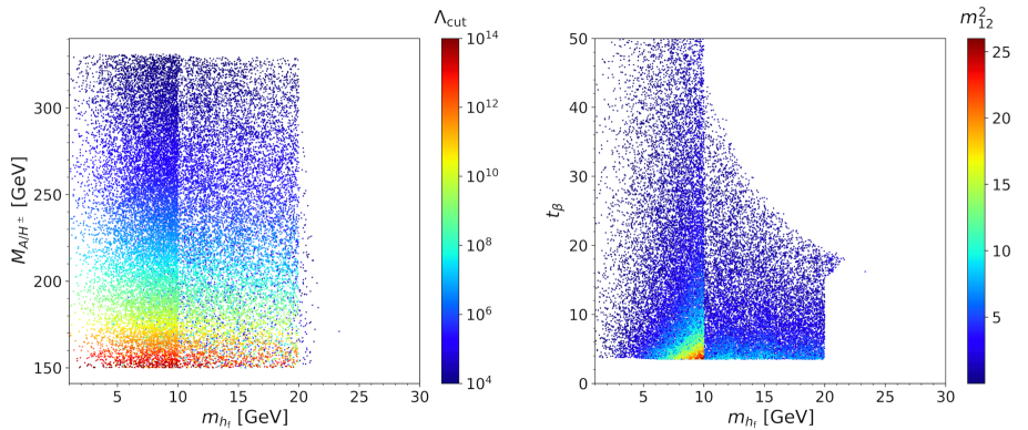
Figure 1: $M_{H^{\pm}}$ versus $m_{h_{\rm f}}$ with a color-code of $\Lambda_{\rm cut}$ in GeV (left panel), and $t_{\beta}$ versus $m_{h_{\rm f}}$ with a color-code of $m_{12}^{2}$ in units of ${\rm GeV}^{2}$ (right panel). All depicted parameter points satisfy the complete set of theoretical and experimental constraints. The parameter points are ordered by ascending values of $\Lambda_{\rm cut}$ in the left panel and $m_{12}^{2}$ in the right panel.

Now we investigate the characteristics of the parameter points satisfying all imposed constraints. In Figure 1, we present $M_{H^{\pm}}$ versus $m_{h_{\rm f}}$ with the color code of $\Lambda_{\rm cut}$ (left panel), and $t_{\beta}$ versus $m_{h_{\rm f}}$ with the color code of $m_{12}^{2}$ (right panel). For visualization clarity, we have ordered the parameter points by ascending values of $\Lambda_{\rm cut}$ in the left panel and $m_{12}^{2}$ in the right panel. This stacking method ensures that points with lower $\Lambda_{\rm cut}$ (or $m_{12}^{2}$) are positioned underneath Kang:2022mdy .

Turning to the $M_{A/H^{\pm}}$ versus $m_{h_{\rm f}}$ plot, we notice several distinct features. First, the density of viable parameter points varies noticeably with the $m_{h_{\rm f}}$ value. Specifically, the number of viable parameter points per unit mass for the intervals $[1,10]{\;{\rm GeV}}$, $[10,20]{\;{\rm GeV}}$, and $[20,30]{\;{\rm GeV}}$ has a ratio of 1 : 0.71 : 0.0058. These significant variations arise from the following direct search constraints:

• The measurement of $pp\to{h_{\rm SM}}\to h_{\rm f}h_{\rm f}\to 4\gamma$ by the ATLAS Collaboration significantly constrains the parameter space for $m_{h_{\rm f}}\in[10,30]{\;{\rm GeV}}$ Aad:2015bua .

• The examination of ${e^{+}e^{-}}\to h_{\rm f}Z\to{\gamma\gamma}Z$ by the ALEPH Collaboration eliminates nearly all parameter points in $m_{h_{\rm f}}\in[20,30]{\;{\rm GeV}}$ ALEPH:2002gcw .

Considering the markedly higher survival percentages, the mass range of $m_{h_{\rm f}}\in[1,10]{\;{\rm GeV}}$ warrants thorough investigation, an endeavor not yet undertaken in existing literature. The second notable feature is the presence of the upper bound on $M_{A/H^{\pm}}$, approximately at $330{\;{\rm GeV}}$. This upper bound exhibits a tendency to decrease as $\Lambda_{\rm cut}$ increases: when $\Lambda_{\rm cut}>100{\;{\rm TeV}}$, the upper threshold reduces to $M_{A/H^{\pm}}\lesssim 280{\;{\rm GeV}}$. These features hold promising implications for the HL-LHC, where the center-of-mass energy of $14{\;{\rm TeV}}$ offers a favorable environment for producing $H^{\pm}$.

In the $t_{\beta}$ versus $m_{h_{\rm f}}$ plot, three significant features stand out. First, lower bounds on $t_{\beta}$ emerge, characterized by $t_{\beta}\gtrsim 4$. This happens because the Yukawa couplings of the BSM Higgs bosons increase as $t_{\beta}$ decreases, as illustrated in Equation 5. The second salient feature is an evident transition at $m_{h_{\rm f}}\simeq 10{\;{\rm GeV}}$. Beneath this threshold, the distribution of permissible parameter points uniformly spans the $t_{\beta}\in[4,50]$ range. For $m_{h_{\rm f}}>10{\;{\rm GeV}}$, however, there is an upper limit on $t_{\beta}$, progressively declining as $m_{h_{\rm f}}$ increases. This transition around $m_{h_{\rm f}}=10{\;{\rm GeV}}$ stems from the notably light mass of $h_{\rm f}$, leading to decay products in high-energy colliders that are challenging to discern. Finally, the $m_{12}^{2}$ distribution primarily leans towards the lower end, peaking around $26{\;{\rm GeV}}^{2}$. This small $m_{12}^{2}$ hints the approximate preservation of $Z_{2}$ parity in the fermiophobic type-I, because only the $m_{12}^{2}$ term breaks $Z_{2}$ parity.

Given these characteristics of the fermiophobic type-I model, we concentrate on the following mass range for $h_{\rm f}$:

$$m_{h_{\rm f}}\in[1,10]{\;{\rm GeV}}.$$ (8)

In subsequent discussions and investigations, we will refer to $h_{\rm f}$ within this mass range as a “very light” $h_{\rm f}$.

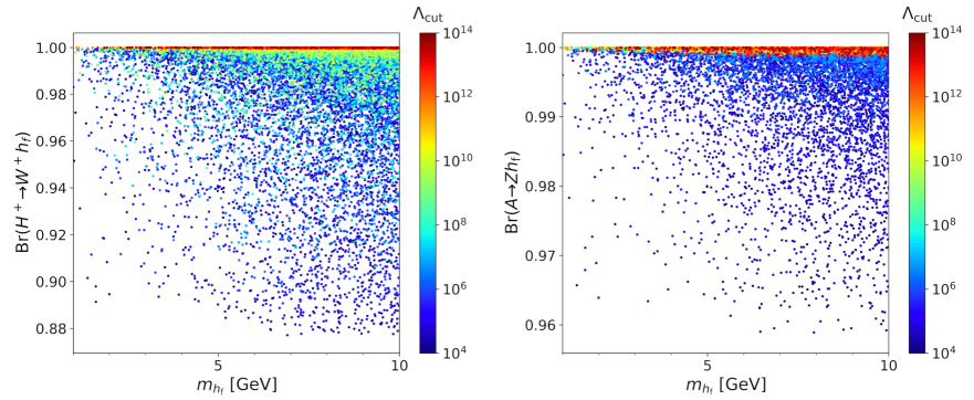
Figure 2: $\text{Br}(H^{\pm}\to h_{\rm f}W^{\pm})$ versus $m_{h_{\rm f}}$ (left panel) and $\text{Br}(A\to h_{\rm f}Z)$ versus $m_{h_{\rm f}}$ (right panel). The color code denotes the cutoff scale $\Lambda_{\rm cut}$ in units of GeV.

Given the distinct characteristics of the fermiophobic type-I model, our attention is directed towards the discovery potential of the the HL-LHC for the very light $h_{\rm f}$. Central to this are its decay modes and production channels. The decay pattern for this particle is unambiguous, with $\text{Br}(h_{\rm f}\to{\gamma\gamma})\simeq 100\%$. Its primary production mechanisms at the LHC occur in association with other BSM Higgs bosons, specifically $pp\to W^{*}\to h_{\rm f}H^{\pm}$ and $pp\to Z^{*}\to h_{\rm f}A$ Kim:2022nmm ; Kim:2023lxc . As a result, the final states arising from these production avenues are intrinsically tied to the decay patterns of $H^{\pm}$ and $A$.

In Figure 2, we depict $\text{Br}(H^{\pm}\to W^{\pm}h_{\rm f})$ versus $m_{h_{\rm f}}$ (left panel) and $\text{Br}(A\to Zh_{\rm f})$ versus $m_{h_{\rm f}}$ (right panel) across all the viable parameter points, with the color codes signifying $\Lambda_{\rm cut}$ values in GeV. Notably, $H^{\pm}\to W^{\pm}h_{\rm f}$ and $A\to h_{\rm f}Z$ surface as the predominant decay channels, with $\text{Br}(H^{\pm}\to W^{\pm}h_{\rm f})$ and $\text{Br}(A\to Zh_{\rm f})$ surpassing 88% and 96%, respectively. A high cutoff scale, such as $\Lambda_{\rm cut}\sim 10^{14}{\;{\rm GeV}}$, results in nearly 100% branching ratios for both $H^{\pm}\to h_{\rm f}W^{\pm}$ and $A\to h_{\rm f}Z$. Hence, two primary candidates for discovery channels present themselves: $pp\to h_{\rm f}H^{\pm}(\to h_{\rm f}W^{\pm})$ and $pp\to h_{\rm f}A(\to h_{\rm f}Z)$. Considering the dominant charged-current production and the larger branching ratio of the leptonic decays of $W^{\pm}$ compared to $Z$, we propose the following as the golden channel to probe the very light $h_{\rm f}$:

$$pp\to W^{*}\to h_{\rm f}H^{\pm}(\to h_{\rm f}W^{\pm})\to{\gamma\gamma}+{\gamma\gamma}+\ell^{\pm}{E_{T}^{\rm miss}},$$ (9)

where $\ell^{\pm}=e^{\pm},\mu^{\pm}$. In our comprehensive analysis, we also incorporate the decay mode $W^{\pm}\to\tau^{\pm}\nu$, which is subsequently followed by $\tau^{\pm}\to\ell^{\pm}\nu\nu$. The corresponding Feynman diagram is depicted in Figure 3.

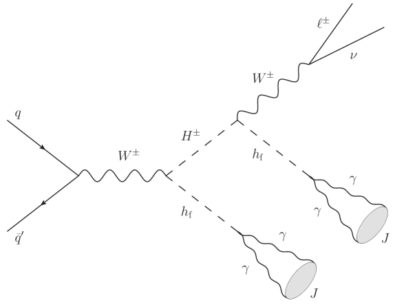
Figure 3: Feynman diagram for the signal process $pp\to W^{*}\to h_{\rm f}H^{\pm}(\to h_{\rm f}W^{\pm})\to{\gamma\gamma}+{\gamma\gamma}+\ell^{\pm}\nu$. As the two photons from the $h_{\rm f}$ decay are highly collimated, they are probed as a single jet $J$.

II.3 Signature of the golden channel $pp\to h_{\rm f}H^{\pm}$

Let us now present the parton-level cross section of the proposed golden channel for $h_{\rm f}$. Initially, we generated the Universal FeynRules Output (UFO) Degrande:2011ua for the fermiophobic type-I through FeynRules Alloul:2013bka . Incorporating this UFO file into MadGraph5-aMC@NLO Alwall:2011uj , we determined the cross-sections of $pp\to H^{\pm}h_{\rm f}$ at the 14 TeV LHC. For the parton distribution function, we adopted the NNPDF31_lo_as_0118 set NNPDF:2017mvq . The branching ratios of $h_{\rm f}$ and $H^{\pm}$ were obtained from 2HDMC Eriksson:2009ws , and subsequently multiplied by the cross-sections.

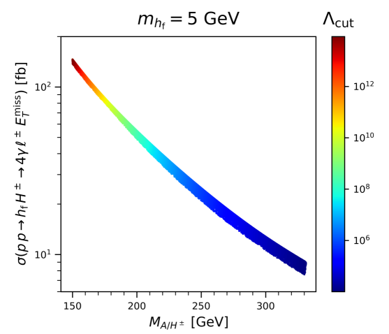
Figure 4: Parton-level cross sections of $pp\to h_{\rm f}H^{\pm}(\to h_{\rm f}W^{\pm})\to 4\gamma\,\ell^{\pm}{E_{T}^{\rm miss}}$ at the 14 TeV LHC, about $M_{H^{\pm}}$. The color code represents the cutoff scale $\Lambda_{\rm cut}$. Here, we set $m_{h_{\rm f}}=5{\;{\rm GeV}}$.

In Figure 4, the scatter plot shows the parton-level cross sections for $m_{h_{\rm f}}=5{\;{\rm GeV}}$ against the charged Higgs boson mass, spanning all viable parameter points. The color code represents $\Lambda_{\rm cut}$. An expected correlation appears between the cross section and $M_{H^{\pm}}$: as $M_{H^{\pm}}$ increases, $\sigma_{\rm tot}$ decreases. Additionally, for a given $M_{H^{\pm}}$, the cross sections across all viable parameter points are nearly constant, with deviations of less than 10%. A compelling feature is the substantial size of the signal cross section. Even the minimum cross section, encountered when $M_{H^{\pm}}\simeq 330{\;{\rm GeV}}$, reaches a significant $\sim 7{\;{\rm fb}}$.

Despite these considerable signal cross sections, distinguishing the signal from the background at the HL-LHC remains a challenge. At first glance, a final state comprised of four photons, a lepton, and missing transverse energy might seem to suppress major QCD backgrounds. But the reality is more intricate. When the $h_{\rm f}$ decays into two photons at high-energy colliders, the resulting photons are not typically isolated because they are tightly collimated within a radius of $\Delta R<0.4$. Here $\Delta R$ is the angular distance, given by $\Delta R=\sqrt{(\Delta\eta)^{2}+(\Delta\phi)^{2}}$. Still, these photons register an energy deposit in the calorimeters, eventually being recognized and grouped as a jet. This leads to substantial QCD backgrounds.

To better elucidate how the detector processes photons, let us briefly review the photon isolation criteria adopted by the Delphes. Consider a photon candidate P, a stable particle that deposits its energy into the electromagnetic calorimeter (ECAL), while leaving no trace in the tracker. For P to be recognized as a photon, it should be sufficiently isolated from neighboring particles. In Delphes, this isolation is determined using the criterion $I(\mathtt{P})>I_{\rm min}$. Here, the isolation variable $I(\mathtt{P})$ is expressed as:

$$I(\mathtt{P})=\dfrac{\sum_{i\neq\mathtt{P}}^{\Delta R<R_{\gamma}}p_{T}^{i}}{p_{T}^{\mathtt{P}}},$$ (10)

where the numerator represents the combined transverse momenta of all particles (excluding P) that fall within a cone of radius $R_{\gamma}$ centered around P. In the delphes_card_HLLHC.tcl utilized in subsequent analysis, the default settings are $I_{\rm min}=0.1$ and $R_{\gamma}=0.3$.

In Delphes, the photon isolation is evaluated concurrently with jet clustering. This procedure involves clustering EflowPhoton, EflowNeutralHadrons, and EflowChargedHadrons according to the energy flow algorithm. Once this process concludes, the definitive identification for P is set. If P satisfies the photon isolation criteria, it is recognized as a photon. Conversely, if P fail the criteria, it is designated as a jet.

To demonstrate our claim that the two photons from $h_{\rm f}\to{\gamma\gamma}$ are more likely to be recognized as a single jet, we conducted a comprehensive detector simulation for the signal with $m_{h_{\rm f}}=5{\;{\rm GeV}}$, $M_{A/H^{\pm}}=150{\;{\rm GeV}}$, and $\text{Br}(H^{\pm}\to h_{\rm f}W^{\pm})=\text{Br}(h_{\rm f}\to{\gamma\gamma})=1$. Parton showering and hadronization were integrated using Pythia version 8.309 Bierlich:2022pfr . We employed Delphes high-luminosity card delphes_card_HLLHC.tcl. For jet clustering, FastJet version 3.3.4 Cacciari:2011ma , deploying the anti-$k_{T}$ algorithm Cacciari:2008gp , was utilized for the jet radius of $R=0.4$. At this stage, we opted not to consider pileup effects.

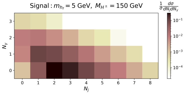
Figure 5: The distribution of photon multiplicity versus jet multiplicity for the signal process $pp\to h_{\rm f}H^{\pm}\to{\gamma\gamma}{\gamma\gamma}\,\ell^{\pm}{E_{T}^{\rm miss}}$ following the detector simulation at the 14 TeV LHC. The color code indicates the normalized number of events. Parameters are set as $m_{h_{\rm f}}=5{\;{\rm GeV}}$, $M_{A/H^{\pm}}=150{\;{\rm GeV}}$, and $\text{Br}(H^{\pm}\to h_{\rm f}W^{\pm})=\text{Br}(h_{\rm f}\to{\gamma\gamma})=1$.

In Figure 5, we present the photon multiplicity versus the jet multiplicity for the signal process at the detector level, using a color code to represent the normalized number of events. These results are derived from $5\times 10^{5}$ events at the generation level. The findings in Figure 5 are striking. The signal event, which includes four photons at the parton level, results in a markedly different outcome at the detector level. Approximately 70% of events fall under $N_{\gamma}=0$, while around 26% are categorized as $N_{\gamma}=1$. Events with $N_{\gamma}=2$ are scarce. Instead, the majority of signal events manifest as two jets.

Background	Cross section [pb]	$n_{\rm gen}$	Background	Cross section [pb]	$n_{\rm gen}$
$W^{\pm}(\to L^{\pm}\nu)jj$	$3.54\times 10^{3}$	$5\times 10^{8}$	$W^{\pm}Z$	$3.16\times 10$	$3\times 10^{6}$
$Z(\to L^{+}L^{-})jj$	$2.67\times 10^{2}$	$5\times 10^{7}$	$Z(\to L^{+}L^{-})j\gamma$	$2.09$	$10^{6}$
${t\bar{t}}(\to{b\bar{b}}W_{L\nu}W_{jj})$	$1.23\times 10^{2}$	$1.2\times 10^{7}$	$ZZ$	$1.18\times 10$	$10^{6}$
$W^{\pm}(\to L^{\pm}\nu)j\gamma$	$2.53\times 10$	$3\times 10^{6}$	$W^{\pm}(\to L^{\pm}\nu){\gamma\gamma}$	$3.28\times 10^{-2}$	$10^{6}$
${W^{+}W^{-}}$	$8.22\times 10$	$9\times 10^{6}$	$Z(\to L^{+}L^{-}){\gamma\gamma}$	$1.12\times 10^{-2}$	$10^{6}$

Table 1: Parton-level cross sections of the backgrounds at the 14 TeV LHC, where $L^{\pm}$ denotes $e^{\pm},\mu^{\pm},$ or $\tau^{\pm}$. The number of generated events, denoted as $n_{\rm gen}$, is also provided.

As the final state includes two jets, various backgrounds arise. We take into account a total of ten background processes: $W^{\pm}(\to L^{\pm}\nu)jj$, $Z(\to L^{+}L^{-})jj$, ${t\bar{t}}(\to{b\bar{b}}W_{L\nu}W_{jj})$, $W^{\pm}(\to L^{\pm}\nu)j\gamma$, ${W^{+}W^{-}}$, $W^{\pm}Z$, $Z(\to L^{+}L^{-})j\gamma$, $ZZ$, $W^{\pm}(\to L^{\pm}\nu){\gamma\gamma}$, and $Z(\to L^{+}L^{-}){\gamma\gamma}$. Here, $L^{\pm}$ represents $e^{\pm},\mu^{\pm},$ or $\tau^{\pm}$. Given that our signal process includes either one electron or one muon, we have incorporated the leptonic decays of $W^{\pm}$ and $Z$ into some dominant backgrounds.

In Table 1, we summarize the parton-level cross sections for the ten background processes at the 14 TeV LHC, applying generation-level cuts of $p_{T}^{j}>20{\;{\rm GeV}}$, $p_{T}^{L,\gamma}>10{\;{\rm GeV}}$, $|\eta_{j}|<5$, $|\eta_{L,\gamma}|<2.5$, and $\Delta R_{ii^{\prime}}>0.4$ where $i$ and $i^{\prime}$ include all the particles in the final state. Due to the considerable differences in the cross sections among these background processes, we produce different event counts at the generation level, represented by $n_{\rm gen}$ in Table 1. Notably, the background cross sections significantly exceed the signal cross section. If the analysis only considers collective objects like jets in the final state, distinguishing the signal from the backgrounds becomes almost infeasible. Consequently, devising a strategy targeting diphoton jets is pivotal for detecting the signal at the HL-LHC.

III Jet subparticles and pileups

In the previous section, we illustrated that the four photons in our signal process, $pp\to h_{\rm f}h_{\rm f}W^{\pm}\to 4\gamma W^{\pm}$, are predominantly tagged as two jets, not isolated photon entities. Given that these photons exist as subparticles within a jet, distinguishing this unique diphoton jet from a standard QCD jet necessitates a thorough analysis of the jet’s subparticles. To enable this differentiation, we employ the EFlow objects within jets in the Delphes framework. These EFlow objects are divided into three categories: EflowPhoton, EflowNeutralHadrons, and EeflowChargedHadrons, with each type determined by tracker and tower information. The tracker identifies charged particles through their characteristic ionization patterns within its system, while tower data focus on energy deposits in the calorimeter.

To enhance our understanding, let us revisit the interactions of particles within calorimeters. Photons, when passing through the electromagnetic calorimeter (ECAL), trigger an energy dispersion across its layers. Hadrons, on the other hand, deposit energy differently depending on their type. Neutral pions, for instance, decay promptly into a pair of photons, largely concentrating their energy within the ECAL. Meanwhile, stable hadrons like neutrons and charged pions predominantly channel their energy to the hadron calorimeter (HCAL). A notable scenario occurs with long-lived hadrons, such as Kaons and $\Lambda$ baryons. With a decay length around 10 mm, they interact with both the ECAL and HCAL, resulting in a division of energy deposit as $f_{\rm ECAL}=0.3$ and $f_{\rm HCAL}=0.7$.

Yet, when it comes to utilizing jet subparticles, the issue of pileup poses a formidable challenge. Pileup, a byproduct of the high luminosity in hadron colliders, results from multiple proton-proton collisions within a single bunch crossing. At the HL-LHC, where roughly 200 pileup events are standard, discerning the diphoton jet from a QCD jet becomes intricate due to the flood of pileup-induced particles. Therefore, it is crucial to effectively subtract pileups in our analysis.

Several methods for pileup subtraction have been advanced, such as the jet vertex fraction TheATLAScollaboration:2013pia , charged hadron subtraction (CHS) CMS:2014ata ; Kirschenmann:2014dla , the Puppi method Bertolini:2014bba , and the SoftKiller method Cacciari:2014gra . In our exploration, we cast a special focus on CHS and SoftKiller. The CHS technique leverages the capability of the detector to determine the vertex distance of charged tracks relative to the primary vertex. In contrast, SoftKiller is a fast event-level pileup subtraction tool, relying on a particle’s transverse momentum to estimate the probability of being a pileup Catani:1993hr ; Ellis:1993tq .

Exploring the advantages of CHS and SoftKiller, we propose an optimal combination: a hybrid strategy named CHS+SK₀. This method first uses CHS to eliminate charged pileup particles, specifically targeting those with a vertex distance greater than $0.1\,\rm{mm}$. Following this, SoftKiller comes into play, removing pileup photons and neutral hadrons that fall below a certain transverse momentum threshold. To avoid overcorrection, we have carefully configured SoftKiller to bypass charged hadrons.

Before showcasing the impressive performance of CHS+SK₀, it is necessary to outline the crucial simulation steps involved. We need to make two important changes to the Delphes settings: first, we remove the pileup subtractors, and second, we turn off the unique object finder module. (However, we ensure that calculations for electron and muon isolation remain intact.) Following these adjustments, the refined output from Delphes is directed to a pileup subtraction module. In the final phase, jet clustering is executed.

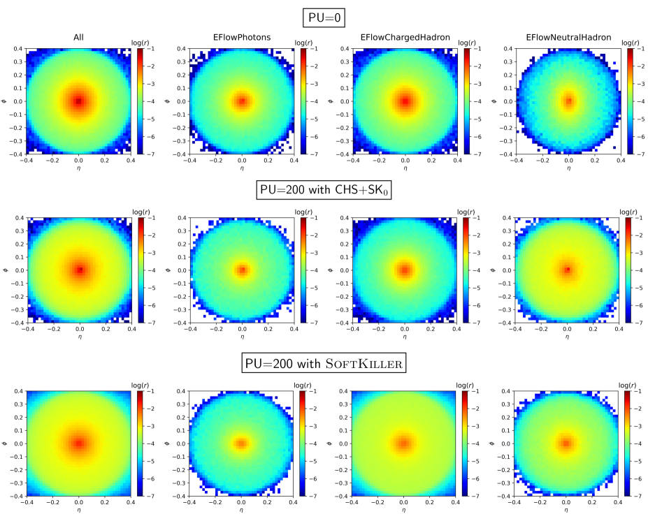
Figure 6: Jet images of the $W^{\pm}jj$ background, where the color scale indicates the logarithm of the ratio of subparticle $p_{T}$ to the mother jet’s $p_{T}$. We examine three pileup subtraction scenarios: no pileup (upper panels), 200 pileups using the CHS+SK₀ subtraction method (middle panels), and 200 pileups using the SoftKiller (lower panels). The presentation spans four distinct jet image types: total jet images (first column), EflowPhotons (second column), EflowNeutralHadrons (third column), and EflowChargedHadrons (fourth column).

We now turn our attention to demonstrating the exceptional performance of CHS+SK₀, utilizing jet images to provide a visual representation of the $p_{T}$ distribution of jet subparticles across a $\eta\times\phi$ grid. In Figure 6, jet images for the leading jet from the $W^{\pm}jj$ background are presented, derived from an extensive sample of $10^{5}$ events.

Preprocessing involves translation and normalization techniques, as outlined in Ref. Ren:2021prq . We then sum the transverse momenta of all the subparticles within the jet and represent the intensity using $\log r$, where $r$ is the ratio of the subparticle’s $p_{T}$ to the mother jet’s $p_{T}$. The $\log r$ information is distributed across the recalibrated $\eta$ and $\phi$ coordinates of each subparticle, which are now positioned relative to their mother jet. Here, we have adopted a pixel size of $\Delta\eta\times\Delta\phi=0.02\times 0.02$, reflecting the resolution of the simulated CMS electromagnetic calorimeter.

Equipped with these jet images, we are ready to conduct a comprehensive comparison between the CHS+SK₀ and SoftKiller subtraction methods. In Figure 6, we explore three scenarios of pileups. The top panels present jet images in the absence of pileups, providing a reference for our pileup subtraction efforts. The middle and bottom panels, on the other hand, display jet images with 200 pileups, processed using the CHS+SK₀ and SoftKiller subtraction methods, respectively.

Further breaking down our analysis, we categorize it into four distinct channels, each illustrated column-wise: total jet, EflowPhotons, EflowChargedHadrons, and EflowNeutralHadrons. As Figure 6 vividly demonstrates, the CHS+SK₀ method significantly outperforms its counterpart, particularly in the efficient removal of charged pileup hadrons. This leads us to opt for the CHS+SK₀ subtraction technique for our subsequent analyses, incorporating all 200 pileup events.

Finally, we establish clear definitions for our terminology related to jets:

Jet ($J$):

A jet encompasses all physical entities that deposit energy in the calorimeters and undergo clustering by a jet algorithm. It is represented as $J$.

Diphoton Jet ($J_{\gamma\gamma}$):

A clustered jet is termed a diphoton jet if its two leading subparticles are EFlowPhotons. We denote this as $J_{\gamma\gamma}$.

QCD Jet ($j$):

A QCD jet, stemming from quarks or gluons, is represented as $j$.

Subparticle ($s_{ij}$):

Each EFlow object inside a jet is referred to as a subparticle. The notation $s_{ij}$ denotes the $i$-th subparticle in the $j$-th jet. Both jets and subparticles are arranged in descending order of their $p_{T}$.

IV Cut-Based Analysis

BP no.	$m_{h_{\rm f}}$	$M_{A/H^{\pm}}$	$s_{\beta-\alpha}$	$m_{12}^{2}$ [GeV2]	$t_{\beta}$
BP-1	$1{\;{\rm GeV}}$	$150{\;{\rm GeV}}$	$-0.123$	$0.0786$	8.06
BP-2		$175{\;{\rm GeV}}$	$-0.0909$	$0.0400$	11.0
BP-3		$200{\;{\rm GeV}}$	$-0.0929$	$0.0813$	10.7
BP-4		$250{\;{\rm GeV}}$	$-0.0941$	$0.0494$	10.6
BP-5		$300{\;{\rm GeV}}$	$-0.0985$	$0.0237$	10.1
BP-6		$331{\;{\rm GeV}}$	$-0.0974$	$0.0634$	10.2
BP-7	$5{\;{\rm GeV}}$	$150{\;{\rm GeV}}$	$-0.0737$	$0.305$	13.5
BP-8		$175{\;{\rm GeV}}$	$-0.0922$	$2.20$	10.8
BP-9		$200{\;{\rm GeV}}$	$-0.0983$	$1.93$	10.1
BP-10		$250{\;{\rm GeV}}$	$-0.0907$	$1.99$	11.0
BP-11		$300{\;{\rm GeV}}$	$-0.0984$	$1.84$	10.1
BP-12		$331{\;{\rm GeV}}$	$-0.0920$	$2.17$	10.8
BP-13	$10{\;{\rm GeV}}$	$150{\;{\rm GeV}}$	$-0.0748$	$1.17$	13.3
BP-14		$175{\;{\rm GeV}}$	$-0.0993$	$1.70$	10.0
BP-15		$200{\;{\rm GeV}}$	$-0.0919$	$0.973$	10.8
BP-16		$250{\;{\rm GeV}}$	$-0.0974$	$0.851$	10.2
BP-17		$300{\;{\rm GeV}}$	$-0.0917$	$0.0396$	10.9
BP-18		$328.3{\;{\rm GeV}}$	$-0.0979$	$1.15$	10.2

Table 2: Benchmark points for the very light $h_{\rm f}$. All the parameter points satisfy the theoretical and experimental conditions.

In this section, we perform a signal-to-background analysis using the traditional cut-based approach. Our primary goal is to attain high signal significances across the entire parameter space for the very light $h_{\rm f}$. To achieve this, we analyze 18 benchmark parameter points, as listed in Table 2. For each signal benchmark point, we generate $3\times 10^{6}$ events. Additionally, we consider the ten background processes specified in Table 1. All events are processed through Pythia8 and Delphes, employing the Delphes configuration outlined in the preceding section.

With our simulated data set ready, we implement the basic selection criteria as follows:

• There must be exactly one lepton with $p_{T}^{\ell}>20{\;{\rm GeV}}$ and $|\eta_{\ell}|<2.5$.

• The leading jet is required to satisfy $p_{T}^{J_{1}}>50{\;{\rm GeV}}$ and $|\eta_{J_{1}}|<2.5$.

• The subleading jet should fulfill the conditions $p_{T}^{J_{2}}>30{\;{\rm GeV}}$ and $|\eta_{J_{2}}|<2.5$.

• The missing transverse energy should exceed ${E_{T}^{\rm miss}}>10{\;{\rm GeV}}$.

In pursuit of optimizing signal significances, we highlight two distinguishing characteristics of our signal: (i) the two leading subparticles in two leading jets are predominantly EFlowPhotons; (ii) these leading subparticles contribute significantly to the transverse momentum of their mother jet.

Figure 7: $P(h_{\rm f}\to J_{\gamma\gamma})$ and $P(j\to J_{\gamma\gamma})$ as functions of $p_{T}^{J}$, for the leading jet in the left panel and the subleading jet in the right panel. $P(h_{\rm f}\to J_{\gamma\gamma})$ represents the probability of two photons from $h_{\rm f}$ being identified as a diphoton jet, while $P(j\to J_{\gamma\gamma})$ is the rate of a QCD jet tagged as a diphoton jet in the $W^{\pm}jj$ background. The red, green, and orange lines depict signal results for benchmark points BP-1, BP-7, and BP-13, respectively.

To highlight the first characteristic, we present the probabilities $P(h_{\rm f}\to J_{\gamma\gamma})$ and $P(j\to J_{\gamma\gamma})$ against the $p_{T}$ of the mother jet in Figure 7. Results for the leading and subleading jets are presented in the left and right panels, respectively. $P(h_{\rm f}\to J_{\gamma\gamma})$ represents the probability of the two photons from an $h_{\rm f}$ decay being identified as a diphoton jet, with the red, green, and orange lines corresponding to benchmark points BP-1, BP-7, and BP-13, respectively. On the other hand, $P(j\to J_{\gamma\gamma})$ denotes the rate at which a QCD jet is misidentified as a diphoton jet in the $W^{\pm}jj$ background.

For the signal, the probability $P(h_{\rm f}\to J_{\gamma\gamma})$ remains substantial, consistently surpassing 40% when $p_{T}^{J}\geq 50{\;{\rm GeV}}$. However, the relationship between this probability and $p_{T}^{J}$ varies with $m_{h_{\rm f}}$. For BP-7 ($m_{h_{\rm f}}=5{\;{\rm GeV}}$) and BP-13 ($m_{h_{\rm f}}=10{\;{\rm GeV}}$), the probability rises with increasing $p_{T}^{J}$, reaching approximately 85%. In contrast, BP-1 ($m_{h_{\rm f}}=1{\;{\rm GeV}}$) shows a distinct pattern: an initial increase, followed by a peak, and then a decrease as $p_{T}^{J}$ rises. This behavior can be attributed to the small $m_{h_{\rm f}}$ value in BP-1. Since $R_{\gamma\gamma}\sim 2m_{h_{\rm f}}/p_{T}$, some of the two photons with high $p_{T}^{J}$ are so collimated that they nearly merge into a single EFlowPhoton, making them challenging to identify as a diphoton jet. Nevertheless, the probability value even for BP-1 remains sizable, hovering around 40%. On the other hand, the mistagging rate $P(j\to J_{\gamma\gamma})$ is only a few percent, demonstrating a clear distinction between signal and background.

The second salient feature of the signal is the large ratios of $p_{T}$ of the two leading subparticles to the $p_{T}$ of their mother jet $J$. In the case of the signal, the diphoton jet is mainly composed of two hard photons, resulting in the leading and subleading subparticles holding a considerable share of $p_{T}^{J}$. In contrast, a QCD jet consists of a diverse mix of particles, numbering from tens to well over a hundred. Consequently, it is rare for the two leading subparticles in a QCD jet to occupy a significant portion of $p_{T}^{J}$. To more vividly illustrate this distinction, we define:

$$r_{ij}=\frac{p_{T}^{s_{ij}}}{p_{T}^{J_{j}}}\quad\text{for $i,j=1,2$}.$$ (11)

Figure 8: Normalized distributions of $r_{ij}$ for the signal in BP-7 (red) and the $W^{\pm}jj$ background (blue) after the basic selection. Here, $r_{ij}$ is the $p_{T}$ ratio defined in Equation 11. The left panel presents the results for the leading subparticle, while the right panel focuses on the second-leading subparticle. Solid lines correspond to results for the leading jet, whereas dashed lines represent the subleading jet.

To demonstrate this second feature, we present in Figure 8 the normalized distributions of $r_{ij}$ for both the signal BP-7 (in red) and the $W^{\pm}jj$ background (in blue) after the basic selection. The left panel showcases the $p_{T}$ ratio for the leading subparticle, $r_{1i}$, while the right panel focuses on the subleading subparticle, $r_{2i}$. Solid lines depict results for $J_{1}$, and dashed lines correspond to $J_{2}$.

A primary observation reveals that the $r_{1i}$ value for the signal consistently surpasses 0.5, indicating that the leading subparticle of a diphoton jet contributes almost half of its mother jet’s $p_{T}$. In contrast, the ratio for the $W^{\pm}jj$ background typically remains under 0.5. Nevertheless, a noticeable peak around $r_{1i}\simeq 0.9$ in the $W^{\pm}jj$ background suggests that merely imposing an upper bound on $r_{1i}$ may not sufficiently differentiate the signal from the background. Consequently, we shift our focus to the $r_{2i}$ distributions. While both the signal and background inherently exhibit $r_{2i}<0.5$, the signal’s $r_{2i}$ is notably larger. By imposing a condition of $r_{2i}>0.25$, which corresponds to $r_{1i}<0.75$, we adeptly avoid the subtle peak around $r_{1i}\sim 0.9$ in the $W^{\pm}jj$ background.

Cross sections in units of fb at the 14 TeV LHC with $\mathcal{L}_{\rm tot}=3{\;{\rm ab}^{-1}}$
Cut	BP-7	$W^{\pm}jj$	$Zjj$	${t\bar{t}}$	$W^{\pm}j\gamma$	$\mathcal{S}_{\rm BP-7}^{10\%}$
Basic	34.8	372 622	27 727	32 052	3 047	$1.09\times 10^{-3}$
${E_{T}^{\rm miss}}>50{\;{\rm GeV}}$	29.7	318 407	23 274	27 395	2 610	$9.01\times 10^{-4}$
$r_{11}>0.50$	24.9	102 182	7 843	4 150	1 214	$2.15\times 10^{-3}$
$r_{12}>0.50$	18.7	36 204	2 853	692	541	$4.56\times 10^{-3}$
$r_{21}>0.25$	7.06	4 218	323	62.2	55.8	$1.49\times 10^{-2}$
$r_{22}>0.25$	2.40	840	61.3	8.61	10.1	$2.56\times 10^{-2}$
$J_{1}\to J_{\gamma\gamma}$	2.29	18.6	2.31	0.205	0.467	1.01
$J_{2}\to J_{\gamma\gamma}$	1.98	0.363	0.0589	0.00	0.00849	22.8

Table 3: Cross-section cut-flow chart for BP-7 and the main backgrounds from $W^{\pm}jj$, $Zjj$, ${t\bar{t}}$, and $W^{\pm}j\gamma$ at the 14 TeV LHC. The presented cross sections are in femtobarns (fb). The basic selection criteria and the ratio $r_{ij}$ are detailed in the main text. For calculating the signal significance ($\mathcal{S}$), we take into account a 10% background uncertainty and assume an integrated luminosity ($\mathcal{L}_{\rm tot}$) of $3{\;{\rm ab}^{-1}}$.

Based on the aforementioned two characteristics of the signal, we devise a strategy to optimize the signal significance using a cut-based analysis. The cut-flow chart in Table 3 outlines the cross sections for the signal and the four main backgrounds—$W^{\pm}jj$, $Zjj$, ${t\bar{t}}$, and $W^{\pm}j\gamma$—at the 14 TeV LHC. We have selected BP-7 as the representative benchmark point for detailed presentation, as it exemplifies the common trends observed across 18 benchmarks. While we have comprehensively analyzed other backgrounds of Table 1, they are omitted in Table 3 due to their negligible impact.

The final column in Table 3 offers the signal significance $\mathcal{S}$, defined by Cowan:2010js :

$$\mathcal{S}=\left[2(N_{\rm S}+N_{\rm B})\log\left(\frac{(N_{\rm S}+N_{\rm B})(N_{\rm B}+\delta_{\rm B}^{2})}{N_{\rm B}^{2}+(N_{\rm S}+N_{\rm B})\delta_{\rm B}^{2}}\right)-\frac{2N_{\rm B}^{2}}{\delta_{b}^{2}}\log\left(1+\frac{\delta_{\rm B}^{2}N_{\rm S}}{N_{\rm B}(N_{\rm B}+\delta_{\rm B}^{2})}\right)\right]^{1/2}.$$ (12)

Here, $N_{\rm S}$ denotes the number of signal events, $N_{\rm B}$ the number of background events, and $\delta_{\rm B}=\Delta_{\rm B}N_{\rm B}$ the background uncertainty yield. We take a 10% background uncertainty ($\Delta_{\rm B}=10\%$).

The results in Table 3 are remarkable. After the basic selection, the four primary backgrounds overwhelm the signal, yielding the significance to an order of magnitude of $10^{-3}$. The cut on the missing transverse energy, pivotal for neutrino tagging, fails to boost the significance due to the presence of a neutrino in the dominant $W^{\pm}jj$ background. The differentiation becomes evident when applying the $p_{T}$ ratio cuts. By enforcing $r_{11}>0.5$ and $r_{12}>0.5$, we retain approximately 63% of the signal events that survive the ${E_{T}^{\rm miss}}>50{\;{\rm GeV}}$ cut, while the backgrounds are diminished to $\mathcal{O}(10^{-3})$. Further imposing $p_{T}$ ratio conditions of $r_{2i}>0.25$ effectively suppresses the backgrounds. Yet, the signal significance remains relatively low, hovering around 2.6%.

The last two selection criteria are decisive. We first require that the leading jet must be a diphoton jet. While this condition significantly reduces the $N_{\rm S}/N_{\rm B}$ ratio, it is not enough to markedly elevate the significance. The final condition that the subleading jet also be a diphoton jet is what truly drives up the significance. When accounting for a 10% background uncertainty, the final significance ascends to 22.8, affirming the discovery of a very light fermiophobic Higgs boson.

Results in the cut-based analysis at the 14 TeV LHC with $\mathcal{L}_{\rm tot}=3{\;{\rm ab}^{-1}}$
	$\sigma_{\rm final}$ [fb]	$\mathcal{S}^{10\%}$		$\sigma_{\rm final}$ [fb]	$\mathcal{S}^{10\%}$		$\sigma_{\rm final}$ [fb]	$\mathcal{S}^{10\%}$
BP-1	1.46	18.5	BP-7	1.98	22.8	BP-13	1.81	21.5
BP-2	1.19	16.1	BP-8	1.68	20.4	BP-14	1.56	19.4
BP-3	0.927	13.4	BP-9	1.37	17.7	BP-15	1.29	17.1
BP-4	0.529	8.71	BP-10	0.900	13.0	BP-16	0.857	12.7
BP-5	0.303	5.49	BP-11	0.582	9.40	BP-17	0.566	9.19
BP-6	0.216	4.09	BP-12	0.457	7.74	BP-18	0.456	7.72

Table 4: Signal cross sections and the significance values after the final selection at the 14 TeV LHC. Calculations are based on a total integrated luminosity of $3{\;{\rm ab}^{-1}}$ and a 10% background uncertainty.

Moving forward, we present the conclusive results for all 18 benchmark points. Table 4 presents the signal cross sections after the final selection and the corresponding significance values at the 14 TeV LHC. These computations are based on a total integrated luminosity of $3{\;{\rm ab}^{-1}}$ and a 10% background uncertainty. The comprehensive suite of cuts in Table 3 is uniformly applied across all benchmark points, avoiding tailored adjustments for specific benchmark points in pursuit of unbiased analysis. The significance values obtained are encouraging. With the exception of BP-6, every benchmark point boasts significance values surpassing 5. Even the notably challenging BP-6 achieves a respectable significance of 4.09.

We observe distinct trends in significance depending on the benchmark points. When holding $m_{h_{\rm f}}$ constant, the significance tends to decrease as $M_{H^{\pm}}$ increases, a reduction primarily due to the smaller signal cross section from the limited kinematic phase space available at higher $M_{H^{\pm}}$ values. Conversely, when fixing $M_{H^{\pm}}$, scenarios with $m_{h_{\rm f}}=5{\;{\rm GeV}}$ consistently yield the highest significances. The slightly reduced significances observed in scenarios with $m_{h_{\rm f}}=10{\;{\rm GeV}}$ result from a subset of signal events producing two photons with $\Delta R>0.4$, which fails to satisfy the criteria for two diphoton jets. On the other hand, scenarios featuring $m_{h_{\rm f}}=1{\;{\rm GeV}}$ consistently exhibit the lowest significance values. This small $m_{h_{\rm f}}$ leads to two collimated photons, causing a significant portion of signal events to not satisfy the two diphoton-jet requirement.

V Mass Reconstruction for $m_{h_{\rm f}}$ and $M_{H^{\pm}}$

In the previous two sections, we underscored the efficacy of our cut-based analysis strategy in achieving robust significance values. Our next aim is to validate that the observed signal indeed originates from the $pp\to h_{\rm f}H^{\pm}\to h_{\rm f}h_{\rm f}W^{\pm}$ process. Precisely identifying the source necessitates the reconstruction of $m_{h_{\rm f}}$ and $M_{H^{\pm}}$. Since $h_{\rm f}$ predominantly decays into two photons, $m_{h_{\rm f}}$ can be reconstructed using the invariant mass of the two photons within a diphoton jet. To reconstruct the mass of the charged Higgs boson, we focus on $M_{T}^{H^{\pm}}$, the transverse mass of $H^{\pm}$ as it decays to ${\gamma\gamma}\ell\nu$.

To initiate the calculation of $M_{T}^{H^{\pm}}$, we first define the four-momentum of the visible components, denoted as $p_{\rm vis}^{\mu}$. A challenge arises due to the presence of an additional diphoton jet in the full scattering process, leading to ambiguity in determining which diphoton jet results from the $H^{\pm}$ decay. To navigate this, we adopt a reasonable assumption: the diphoton jet stemming from the decay of $H^{\pm}$ is the subleading jet. This assumption is based on the observation that the prompt diphoton jet generally exhibits a higher $p_{T}$ than the one involved in the decay chain.

Following this assumption, we establish:

$$p_{\rm vis}^{\mu}=p_{s_{12}}^{\mu}+p_{s_{22}}^{\mu}+p_{\ell}^{\mu}.$$ (13)

The square of the transverse mass of the charged Higgs boson is then defined as:

$$\left(M_{T}^{H^{\pm}}\right)^{2}=m_{\rm vis}^{2}+2\left[E_{T}^{\rm vis}{E_{T}^{\rm miss}}-\vec{p}_{T}^{\rm\;vis}\cdot\vec{E}_{T}^{\rm\,miss}\right],$$ (14)

where $m_{\rm vis}^{2}=p_{\rm vis}\cdot p_{\rm vis}$, $E_{T}^{\rm vis}=\sqrt{m_{\rm vis}^{2}+\left({p}_{T}^{\rm vis}\right)^{2}}$, and $\vec{E}_{T}^{\rm\,miss}=-\sum_{i}\vec{p}_{T}^{\,i}$ with $i$ covering all the observed particles after the pileup subtraction.

In our endeavor to determine $m_{h_{\rm f}}$ and $M_{T}^{H^{\pm}}$, we are confronted with a formidable challenge: obtaining accurate background distributions after imposing the final selection. While the final selection guarantees robust signal significances through a drastic reduction in background events—leaving only 51 events for the $W^{\pm}jj$ background and 4 events for $Zjj$—this scarcity of events impairs our ability to acquire precise distributions for both ${m_{\gamma\gamma}}$ and $M_{T}^{H^{\pm}}$. However, abandoning the final selection is not an option, as the second-to-last cut results in an unacceptably low significance, falling below one. Furthermore, intensifying event generation to amplify the number of background events is impractical, as our computational resources are already maximized, with $5\times 10^{8}$ events generated for $W^{\pm}jj$ and $5\times 10^{7}$ for $Zjj$.

In tackling this challenge, we have developed a novel approach that incorporates the mistagging probability $P(j\to J_{\gamma\gamma})$ as a weighting factor, a method we term the Weighting Factor Method (WFM). To grasp the benefits of WFM, it is instructive to examine the methodology of traditional cut-based analyses. These analyses operate by either retaining or discarding events based on selection criteria, effectively assigning a binary weight of one or zero to each event. While straightforward, this method proves inefficient for analyzing background distributions when the selection efficiency is exceedingly low. For instance, the final selection efficiency for the $W^{\pm}jj$ backgrounds, relative to the basic selection, is an astonishingly sparse $10^{-7}$.

In contrast, our WFM strategically utilizes the continuous nature of the weighting factor $P(j\to J_{\gamma\gamma})$. This approach ensures the inclusion of nearly all pertinent background events, ensuring a thorough representation of the background. For a comprehensive explanation of WFM, including a detailed discussion on how we model $P(j\to J_{\gamma\gamma})$, please refer to Appendix A.

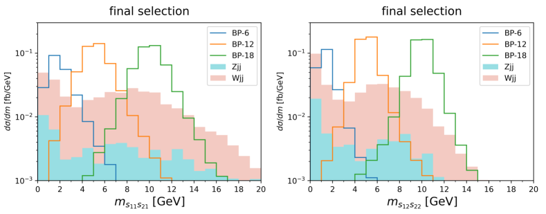
Figure 9: Invariant mass distributions for the two leading subparticles in the leading jet (left panel) and the subleading jet (right panel) at the 14 TeV LHC. All depicted events meet the final selection criteria. For the stacked $W^{\pm}jj$ and $Zjj$ backgrounds, the WFM is utilized. The expected signals for BP-6 (blue), BP-12 (orange), and BP-18 (green) are illustrated with solid lines.

In Figure 9, we depict the distributions of $m_{s_{11}s_{21}}$ (left panel) and $m_{s_{12}s_{22}}$ (right panel) for both signal and background events at the 14 TeV LHC, adhering to the final selection criteria detailed in Table 3. We consider three signal benchmark points with a heavy $M_{H^{\pm}}$: BP-6 (blue), BP-12 (orange), and BP-18 (green). For the signal distributions, we rely on the results from the traditional cut-based analysis, justified by the ample number of signal events remaining post final selection. In addition, we display the results for the two primary backgrounds, $W^{\pm}jj$ and $Zjj$, in the stacked format, using the WFM. We omit other backgrounds here due to their inconsequential contributions following the final selection.

A salient characteristic for the signal in Figure 9 is a distinct resonance peak, for both the leading and subleading jets. This peak closely corresponds to the mass of the fermiophobic Higgs boson. Conversely, the background distributions exhibit two peaks: a sharp one and a more diffuse secondary one. The acute peak, centered at ${m_{\gamma\gamma}}\simeq 0$, is predominantly attributed to light mesons, such as $\pi^{0}$, $\rho$, $\eta$, and $\eta^{\prime}$, which decay into two photons. Meanwhile, the broader peak around ${m_{\gamma\gamma}}\simeq 10{\;{\rm GeV}}$ emerges as background events increasingly mimic the signal after meeting all selection criteria. Nevertheless, the resonance peaks in the diphoton invariant mass distributions are clearly distinguishable from the backgrounds.

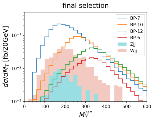
Figure 10: Distributions of the transverse mass of the charged Higgs boson after the final selection at the 14 TeV LHC. The results for the $W^{\pm}jj$ and $Zjj$ backgrounds are displayed in a stacked manner. The expected signals for BP-6 (red), BP-7 (blue), BP-10 (orange), and BP-12 (green) are represented by solid lines.

In Figure 10, we show the transverse mass distribution of the charged Higgs boson. For the signal, four benchmark points are considered: BP-6 (red), BP-7 (blue), BP-10 (orange), and BP-12 (green). Additionally, we showcase the WFM results for the two primary backgrounds, $W^{\pm}jj$ and $Zjj$, in a stacked manner.

The $M_{T}^{H^{\pm}}$ distributions for the signal exhibit a unique wedge-shaped peak, marked by a sudden drop around $M_{T}^{H^{\pm}}\simeq M_{H^{\pm}}$. However, this peak is broader than the well-known distribution shape of $W^{\pm}\to\ell^{\pm}\nu$. This broadening arises from two main factors. First, the long decay chain of $H^{\pm}\to h_{\rm f}W^{\pm}\to{\gamma\gamma}\ell\nu$ introduces inherent uncertainties, especially when measuring the three momenta of the two photons and one lepton. Second, there is ambiguity in determining which diphoton jet originates from the $H^{\pm}$ decay. Despite the broadness, the characteristic shape of the transverse mass distribution is evident in the signal.

On the other hand, the backgrounds show a single, broad hill-shaped peak centered around $180{\;{\rm GeV}}$. This shape evolves as background events increasingly resemble the signal after satisfying all selection criteria. One might worry that the background peak around $180{\;{\rm GeV}}$ could obscure the signal $M_{T}^{H^{\pm}}$ peak when $M_{H^{\pm}}$ is close to 180 GeV. However, as indicated in Table 4, the significance values for $M_{H^{\pm}}=175{\;{\rm GeV}}$ are so high that the $M_{T}^{H^{\pm}}$ signal peaks remain distinct and easily distinguishable from the background contributions.

In conclusion, the mass reconstruction of $m_{h_{\rm f}}$ and $M_{H^{\pm}}$ is feasible, signifying that the combined ${m_{\gamma\gamma}}$ and $M_{T}^{H^{\pm}}$ distributions effectively and distinctly pinpoint the origin of our new signal.

VI Machine Learning Approach for heavy $M_{H^{\pm}}$

In the previous two sections, we underscored the efficacy of our cut-based analysis strategy in achieving robust significance values as well as the mass reconstruction of ${m_{\gamma\gamma}}$ and $M_{H^{\pm}}$. Yet, challenges manifested when addressing the heavy charged Higgs boson. For instance, BP-6 reached a significance of 4.09, which is not convincing enough to confirm the presence of the very light fermiophobic Higgs boson. Hence, in this section, we employ machine learning techniques, with a keen focus on BP-6, BP-12, and BP-18, aiming to enhance the significances. At the parton-level, the total cross sections for these benchmarks are $\sigma_{\rm tot}(\text{BP-6})=9.62{\;{\rm fb}}$, $\sigma_{\rm tot}(\text{BP-12})=9.63{\;{\rm fb}}$, and $\sigma_{\rm tot}(\text{BP-18})=9.83{\;{\rm fb}}$.

Let us begin by discussing the preparation of input features. We formulate two distinct features: the event feature and the subparticle feature. The event feature comprises 21 elements, constructed as follows:

$$\mathbf{v}_{\rm event}= \left[p_{T}^{J_{1}},\eta_{J_{1}},\phi_{J_{1}},m_{J_{1}},p_{T}^{J_{2}},\eta_{J_{2}},\phi_{J_{2}},m_{J_{2}},p_{T}^{\ell},\eta_{\ell},\phi_{\ell},{E_{T}^{\rm miss}},\phi_{\vec{E}_{T}^{\rm miss}},\right.$$ (15)

$$\left.\Delta R_{J_{1}J_{2}},\Delta R_{J_{1}\ell},\Delta R_{J_{2}\ell},\Delta R_{J_{1}{\vec{E}_{T}^{\rm miss}}},\Delta R_{J_{2}{\vec{E}_{T}^{\rm miss}}},\Delta R_{\ell{\vec{E}_{T}^{\rm miss}}},M_{T}^{J_{1}},M_{T}^{J_{2}}\right],$$ (16)

with $M_{T}^{J_{i}}$ ($i=1,2$) representing the transverse mass in Equation 14 using $p_{\rm vis}^{\mu}=p_{J_{i}}^{\mu}+p_{\ell}^{\mu}$. For normalization, the feature elements with a mass dimension are divided by $500{\;{\rm GeV}}$. This list includes the transverse momentum $p_{\text{T}}$, the invariant mass $m_{J_{i}}$, the missing transverse energy ${E_{T}^{\rm miss}}$, and the transverse mass $M_{T}^{J_{i}}$.

The subparticle feature is divided into two vectors associated with $J_{1}$ and $J_{2}$. Each $J_{i}$ category includes the 10 leading subparticles, each characterized by three attributes: $p_{T}$, $\eta$, and $\phi$. As a result, the total dimension of the subparticle feature is $30\times 2$. The coordinates $\eta$ and $\phi$ of a given subparticle are adjusted to be relative to their mother jet. We divide the $p_{T}$ values by $100{\;{\rm GeV}}$ for normalization. To emphasize the photons, other particles (hadrons) are assigned a value of zero for all three attributes.

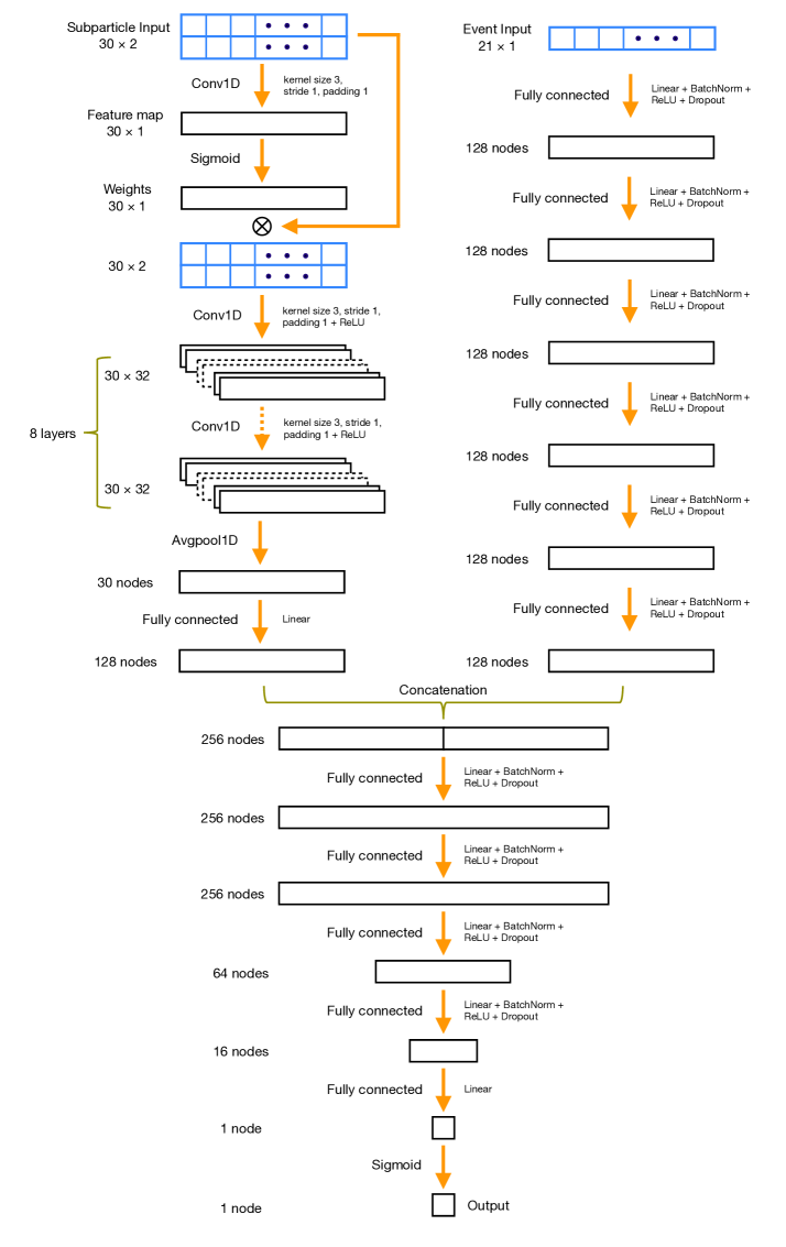
Figure 11: Model architecture of 1D CNN

Our network architecture, illustrated in Figure 11, consists of three main components: a one-dimensional (1D) CNN block and two multilayer perceptrons (MLP1 and MLP2). The 1D CNN block is responsible for processing the subparticle feature, whereas MLP1 handles the event feature. MLP2 merges the outputs from both the 1D CNN and MLP1 to produce the final model prediction. For those interested in the datasets and the detailed operation of the deep learning model, we have made them available on our GitHub repository.

Diving into the details, the 1D CNN block comprises nine 1D convolutional layers. The first layer uses a kernel size of 3 and its output goes through a sigmoid function, which maps the values between 0 and 1. Functioning as attention weights, these values are multiplied by each subparticle input feature. This is a crucial step with a clear purpose: it assigns varying weights to each element within the input features, thereby enhancing the model’s ability to focus on informative parts of the data. The next eight layers are also 1D convolutions with a kernel size of 3, but they include a ReLU activation function to add non-linearity to the model. Following these layers, an average pooling operation and a fully connected layer condense the information into a 128-dimensional feature vector.

MLP1 primarily transforms the event input feature into a 128-dimensional feature vector. This perceptron comprises six fully connected layers, each containing 128 nodes. Following each layer, batch normalization, a ReLU activation function, and a dropout layer with a 50% probability are applied.

MLP2 finally determines the probability that an event is classified as a signal. Its architecture includes five fully connected layers with node counts of 256, 256, 256, 64, and 16, in succession. Each layer is followed by batch normalization, a ReLU activation function, and a dropout layer with a 50% probability. After these five layers, an additional fully connected layer is set in place to produce an one-dimensional feature vector. This vector then undergoes processing via a sigmoid function, yielding the final classification probability as the output.

For optimal model implementation and precision, we utilize the renowned PyTorch deep learning framework paszke2019pytorch . Both training and evaluation processes are expedited using the NVIDIA Titan V GPU. We optimize model parameters with the AdamW optimizer loshchilov2017decoupled , which is set with an initial learning rate of 0.002 and a weight decay of 0.01, based on mini-batches of 512 training samples. Throughout the training phase, which spans 100 epochs, we decrease the learning rate by half every 10 epochs to enhance convergence.

Now let us describe the generation and assignment of our dataset for training and evaluation. To leverage the unique attributes that differentiate the signal from the backgrounds, we enforce additional conditions $p_{T}^{J_{1}}>100{\;{\rm GeV}}$ and $p_{T}^{J_{2}}>80{\;{\rm GeV}}$, after the basic selection. During the training phase, we employ training and validation datasets, each brimming with $6\times 10^{5}$ events. These datasets are evenly split for signals and backgrounds. The signal events are equally divided amongst BP-6, BP-12, and BP-18. For the background events, which originate from ten processes, allocation is proportionate to their respective cross sections.

Central to our training and evaluation processes is the design of our loss function. Our primary goal of enhancing detection significance necessitates efficient background rejection. Accordingly, we have tailored the loss function to inversely correlate with signal significance. For the sake of computational efficiency, we employ $1/Z$ as the loss function, where $Z$ is a concise representation for the significance:

$$Z=\frac{N_{\rm S}}{\sqrt{N_{\rm B}+\delta_{\rm B}^{2}}},$$ (17)

where we take into account a 10% background uncertainty, denoted as $\delta_{\rm B}=0.1N_{\rm B}$.

Upon concluding the training process, we extract the model’s optimal parameters and apply them to our entire test dataset—totaling $1.27\times 10^{8}$ events, consisting of $9\times 10^{6}$ signal events and an overwhelming $1.18\times 10^{8}$ background events. Subsequently, we apply a specified selection threshold $x_{\rm cut}$ on the outputs of all the test samples. Finally we then determine the comprehensive significance metric $\mathcal{S}$ in Equation 12.

Given two threshold options, $x_{\rm cut}=0.5$ and $x_{\rm cut}=0.9$, we present the signal significances for BP-6, BP-12, and BP-18 as follows:

$$\begin{split}x_{\rm cut}=0.5&:\qquad\mathcal{S}_{\text{BP-6}}^{10\%}=\phantom{1}9.0,\quad\mathcal{S}_{\text{BP-12}}^{10\%}=15.4,\quad\mathcal{S}_{\text{BP-18}}^{10\%}=15.0;\\ x_{\rm cut}=0.9&:\qquad\mathcal{S}_{\text{BP-6}}^{10\%}=18.9,\quad\mathcal{S}_{\text{BP-12}}^{10\%}=33.2,\quad\mathcal{S}_{\text{BP-18}}^{10\%}=32.4.\end{split}$$ (18)

The outcomes from our CNN machine learning approach are indeed outstanding. Even with the conservative threshold of $x_{\rm cut}=0.5$, BP-6 now reaches a significance of $9.0$. Furthermore, both BP-12 and BP-18 witness approximately 100% increases in their significances when compared to the results from the cut-based analysis. Opting for the more aggressive threshold of $x_{\rm cut}=0.9$ yields even more enhanced significances. Collectively, these outcomes emphatically demonstrate the effectiveness of our model architecture.

VII Conclusions

We have comprehensively studied the phenomenological signatures associated with a very light fermiophobic Higgs boson $h_{\rm f}$ with a mass range of $m_{h_{\rm f}}\in[1,10]{\;{\rm GeV}}$ at the 14 TeV LHC. The light $h_{\rm f}$ is postulated under the condition $\alpha=\pi/2$ within the inverted Higgs scenario of the type-I two-Higgs-doublet model. Through an exhaustive scan of the parameter space, taking into account theoretical requirements, experimental constraints, and the cutoff scale exceeding 10 TeV, we demonstrated that the $m_{h_{\rm f}}\in[1,10]{\;{\rm GeV}}$ range retains a substantial number of viable parameter points. This is largely attributed to the experimental complexities of detecting the soft decay products of $h_{\rm f}$. Importantly, this mass range results in strictly defined parameter space, ensuring predictable phenomenological signatures. Two standout features of the viable parameter space are: (i) the BSM Higgs bosons have a single dominant decay mode, such as $h_{\rm f}\to{\gamma\gamma}$, $H^{\pm}\to h_{\rm f}W^{\pm}$, and $A\to h_{\rm f}Z$; (ii) $M_{H^{\pm}}$ and $M_{A}$ are relatively light below $\lesssim 330{\;{\rm GeV}}$. Building on these insights, we have proposed a golden channel, $pp\to h_{\rm f}H^{\pm}\to{\gamma\gamma}{\gamma\gamma}\ell\nu$, for exploration of $h_{\rm f}$ at the HL-LHC.

A serious challenge surfaces as the two photons from $h_{\rm f}\to{\gamma\gamma}$ fail to meet the photon isolation criteria, due to their high collimation within $\Delta R<0.4$. As a result, the final state (characterized by four photons) usually manifests as two jets, thereby facing immense QCD backgrounds. To address this, we shifted our focus to the subparticles within the jet, identifiable as EFlow objects within the Delphes framework. This approach facilitates the extraction of information about a subparticle’s type (EflowPhoton, EflowNeutralHadrons, or EflowChargedHadrons), subsequently enabling the probing of diphoton jets. The challenges posed by pronounced pileups, which could blur the distinction between diphoton jets and QCD jets, are effectively addressed by our innovative pileup subtraction method—a hybrid solution combining charged hadron subtraction with SoftKiller.

With the method of probing diphoton jets, we performed the full simulation for signal-to-background analysis at the detector level across 18 benchmark points. A universal strategy was articulated for the cut-based analysis, yielding encouraging outcomes. Except for BP-6, characterized by $m_{h_{\rm f}}=1{\;{\rm GeV}}$ and $M_{H^{\pm}}=330{\;{\rm GeV}}$, all benchmark points exhibited signal significance considerably above 5. For the mass reconstructions of the BSM Higgs bosons, we analyzed both the invariant mass distribution of the two leading subparticles and the transverse mass of the charged Higgs boson, based on events post the final selection. Distinct peaks correlating with $m_{h_{\rm f}}$ and $M_{H^{\pm}}$ were prominently discerned above the background signals. An inherent challenge—securing reliable background distributions with the scarce events post the final selection—is addressed through our pioneering Weighting Factor Method (WFM).

To cover the more challenging regions marked by a heavy charged Higgs boson mass, we employed machine learning techniques. A potent network structure was designed, comprised of a one-dimensional (1D) CNN block followed by two multilayer perceptrons. The efficacy of this model was commendable. With the nominal threshold of $x_{\rm cut}=0.5$, we managed to nearly double the significances for the heavy $M_{H^{\pm}}$ cases.

In this extensive research, we have explored uncharted territories of a very light fermiophobic Higgs boson via diphoton jets. Our approach, harmonizing traditional analyses with innovative methodologies like hybrid pileup subtraction, the WFM, and machine learning, offers novel contributions to the field. We urge the community to consider our findings in the quest for BSM signals.

Appendix A Weighting factor method

In this appendix, we elaborate on the Weighting Factor Method (WFM). Our focus sharpens on the modeling of $P(j\to J_{\gamma\gamma})$ for background processes, where $P(j\to J_{\gamma\gamma})$ represents the probability of a QCD jet misidentified as a diphoton jet. The extreme scarcity of background events that pass the final selection criteria makes this approach crucial for attaining reliable distributions of ${m_{\gamma\gamma}}$ and $M_{T}^{H^{\pm}}$, which necessitate a substantial number of events. Our discussion in this Appendix focuses on the dominant $W^{\pm}jj$ backgrounds, considering that the next dominant $Zjj$ backgrounds contribute to only about 10% of the $W^{\pm}jj$ events.

For clarity in our subsequent discussions, we elucidate some terminologies. The expected number of events corresponding to a specific luminosity is denoted by $N$. In realistic simulations, however, the actual number of generated background events is less than $N$. For distinction, we denote it by $n$. To be more explicit, let us define $E_{\rm cut}$ as the set of events that fulfill a certain “cut”. The number of events meeting this cut is determined by the cardinality of the set $E_{\rm cut}$:

$$n_{\rm cut}\equiv\#E_{\rm cut}.$$ (19)

In the conventional cut-based analysis, the cross section after the final selection is then given by

$$\sigma_{\rm final}^{\text{cut-based}}=\sum_{e\in E_{\rm final}}1\times\frac{\sigma_{\rm tot}}{n_{\rm gen}}=\frac{n_{\rm final}}{n_{\rm gen}}\;\sigma_{\rm tot},$$ (20)

where $\sigma_{\rm tot}$ represents the total cross section at the parton level.

Let us revisit the cut-flow presented in Table 3. Following the basic selection, we have an accumulative sequence of criteria: (i) ${E_{T}^{\rm miss}}>50{\;{\rm GeV}}$; (ii) $r_{11}>0.5$; (iii) $r_{12}>0.5$; (iv) $r_{21}>0.25$; (v) $r_{22}>0.25$; (vi) $J_{1}\to J_{\gamma\gamma}$; (vii) $J_{2}\to J_{\gamma\gamma}$. The $W^{\pm}jj$ backgrounds register counts of $n_{r_{22}}=1.180\times 10^{5}$ and $n_{{\rm final}}=51$, where the condition ${r_{22}}$ represents the accumulated conditions leading up to $r_{22}>0.25$.

Now we unpack how the WFM modifies $\sigma_{\rm final}^{\text{cut-based}}$. Instead of focusing on the background events post the final selection, we shift our attention to the more extensive dataset refined by the $r_{22}$ condition. For each background event $e$ within the set $E_{r_{22}}$, we determine $P_{e}(j_{1}\to J_{\gamma\gamma})$ and $P_{e}(j_{2}\to J_{\gamma\gamma})$ that serve as weight factors. To compute the joint probability using these multipliers, we adopt an assumption: the observation of $j_{1}$ as a diphoton jet remains statistically decoupled from $j_{2}$’s categorization. This implies that scenarios in which both jets are tagged as diphoton jets are derived from the multiplication of their respective weighting factors. Therefore, the cross section following the final selection, under the WFM framework, becomes

$$\sigma_{\rm final}^{\text{WFM}}=\sum_{e\in E_{r_{22}}}P_{e}(j_{1}\to J_{\gamma\gamma})P_{e}(j_{2}\to J_{\gamma\gamma})\times\frac{\sigma_{\rm tot}}{n_{\rm gen}}.$$ (21)

It is important to reiterate: for $\sigma_{\rm final}^{\text{cut-based}}$ in Equation 20, we consider the $n_{\rm final}$ events, while for $\sigma_{\rm final}^{\text{WFM}}$ in Equation 21, we employ the $n_{r_{22}}$ events.

To model $P_{e}(j\to J_{\gamma\gamma})$ in practice, we need to compute the ratio of event counts after the $j\to J_{\gamma\gamma}$ cut to those satisfying the $r_{22}$ cut. Recognizing that $P_{e}(j\to J_{\gamma\gamma})$ would naturally depend on event-specific characteristics like $p_{T}^{j}$, it is pertinent to focus on the event counts within a defined kinematic bin when calculating the ratio. Considering that the magnitude of $P_{e}(j\to J_{\gamma\gamma})$ is on the order of a few percent, a substantial volume of events that satisfy the $r_{22}$ condition must be collected in the reference set. Strategically, we adopt two-dimensional kinematic bins.

For any specific event $e$, we introduce $B_{e}$ as the set of all events within the bin containing $e$. Consequently, the probability of a QCD jet being incorrectly identified as a diphoton jet in event $e$ is given by:

$$P_{e}(j\to J_{\gamma\gamma})=\frac{\#\left(E_{j\to J_{\gamma\gamma}}\cap B_{e}\right)}{\#\left(E_{r_{22}}\cap B_{e}\right)},$$ (22)

where the criteria within $E_{j\to J_{\gamma\gamma}}$ means the combination of the $j\to J_{\gamma\gamma}$ condition with the $r_{22}$ cut.

The advantages of WFM become clear when analyzing kinematic distributions. As an illustration, consider a case where $\#\left(E_{r_{22}}\cap B_{e}\right)=1000$. Using the traditional cut-based method and implementing both $j_{1}\to J_{\gamma\gamma}$ and $j_{2}\to J_{\gamma\gamma}$ conditions, most of the kinematic bins become empty since the joint probability is exceedingly low as $3.8\times 10^{-4}$. It is not feasible to obtain a reliable kinematic distribution in this case. In contrast, utilizing the WFM method, we can expect a projection of roughly 0.38 events post-final selection, enabling reliable distributions.

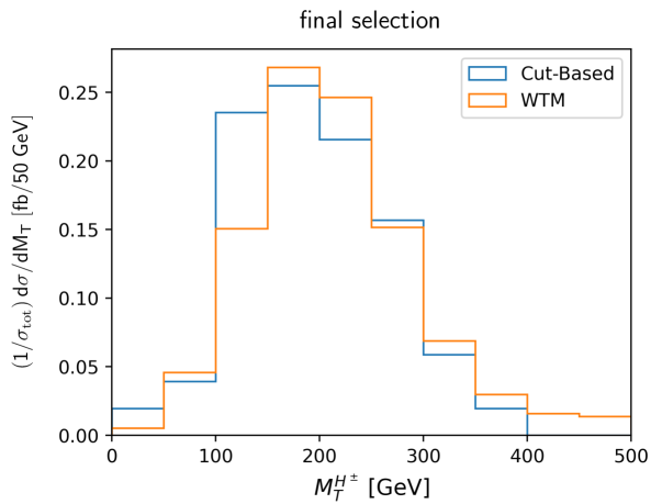
Figure 12: Comparison of the $M_{T}^{H^{\pm}}$ distribution from the $W^{\pm}jj$ background in the cut-based analysis with that in the WTM, after the final selection.

Finally, to confirm the effectiveness of the WFM, we compare its resulting distributions with those from the traditional cut-based analysis. This comparison is meaningful when the cut-based analysis accurately reflects the main features of the true distribution after applying the final selection criteria. However, the $m_{s_{1i}s_{2i}}$ distribution in the $W^{\pm}jj$ background is not suitable for this comparison due to its complexity. Therefore, we consider the $M_{T}^{H^{\pm}}$ distribution for the comparison, which enjoys a simple, smooth hill-like shape.

In Figure 12, we present side-by-side the $M_{T}^{H^{\pm}}$ distribution of the $W^{\pm}jj$ background from the traditional cut-based analysis and its WFM counterpart. The results are post the final selection. Despite the inherent constraints arising from the limited data in the cut-based method, there is a clear resemblance between the two distributions. Both profiles exhibit a smoothly contoured hill shape and almost the same peak positions. This similarity underscores the capability of the WFM to properly represent the $M_{T}^{H^{\pm}}$ distribution. In conclusion, the WFM proves indispensable when tackling huge backgrounds with particularly stringent selection criteria.

References

- (1) ATLAS collaboration, G. Aad et al., Observation of a new particle in the search for the Standard Model Higgs boson with the ATLAS detector at the LHC, Phys. Lett. B 716 (2012) 1–29, [1207.7214].
- (2) CMS collaboration, S. Chatrchyan et al., Observation of a New Boson at a Mass of 125 GeV with the CMS Experiment at the LHC, Phys. Lett. B 716 (2012) 30–61, [1207.7235].
- (3) J. F. Navarro, C. S. Frenk and S. D. M. White, The Structure of cold dark matter halos, Astrophys. J. 462 (1996) 563–575, [astro-ph/9508025].
- (4) G. Bertone, D. Hooper and J. Silk, Particle dark matter: Evidence, candidates and constraints, Phys. Rept. 405 (2005) 279–390, [hep-ph/0404175].
- (5) G. Degrassi, S. Di Vita, J. Elias-Miro, J. R. Espinosa, G. F. Giudice, G. Isidori et al., Higgs mass and vacuum stability in the Standard Model at NNLO, JHEP 08 (2012) 098, [1205.6497].
- (6) S. Dimopoulos and G. F. Giudice, Naturalness constraints in supersymmetric theories with nonuniversal soft terms, Phys. Lett. B 357 (1995) 573–578, [hep-ph/9507282].
- (7) K. L. Chan, U. Chattopadhyay and P. Nath, Naturalness, weak scale supersymmetry and the prospect for the observation of supersymmetry at the Tevatron and at the CERN LHC, Phys. Rev. D 58 (1998) 096004, [hep-ph/9710473].
- (8) N. Craig, A. Katz, M. Strassler and R. Sundrum, Naturalness in the Dark at the LHC, JHEP 07 (2015) 105, [1501.05310].
- (9) A. G. Akeroyd, Fermiophobic Higgs bosons at the Tevatron, Phys. Lett. B 368 (1996) 89–95, [hep-ph/9511347].
- (10) A. G. Akeroyd, Fermiophobic and other nonminimal neutral Higgs bosons at the LHC, J. Phys. G 24 (1998) 1983–1994, [hep-ph/9803324].
- (11) A. G. Akeroyd, Three body decays of Higgs bosons at LEP-2 and application to a hidden fermiophobic Higgs, Nucl. Phys. B 544 (1999) 557–575, [hep-ph/9806337].
- (12) A. Barroso, L. Brucher and R. Santos, Is there a light fermiophobic Higgs?, Phys. Rev. D 60 (1999) 035005, [hep-ph/9901293].
- (13) L. Brucher and R. Santos, Experimental signatures of fermiophobic Higgs bosons, Eur. Phys. J. C 12 (2000) 87–98, [hep-ph/9907434].
- (14) A. G. Akeroyd and M. A. Diaz, Searching for a light fermiophobic Higgs boson at the Tevatron, Phys. Rev. D 67 (2003) 095007, [hep-ph/0301203].
- (15) A. G. Akeroyd, M. A. Diaz and F. J. Pacheco, Double fermiophobic Higgs boson production at the CERN LHC and LC, Phys. Rev. D 70 (2004) 075002, [hep-ph/0312231].
- (16) A. G. Akeroyd, M. A. Diaz and M. A. Rivera, Effect of Charged Scalar Loops on Photonic Decays of a Fermiophobic Higgs, Phys. Rev. D 76 (2007) 115012, [0708.1939].
- (17) A. Arhrib, R. Benbrik, R. B. Guedes and R. Santos, Search for a light fermiophobic Higgs boson produced via gluon fusion at Hadron Colliders, Phys. Rev. D 78 (2008) 075002, [0805.1603].
- (18) E. Gabrielli, B. Mele and M. Raidal, Has a fermiophobic Higgs boson been detected at the LHC?, Phys. Lett. B 716 (2012) 322–325, [1202.1796].
- (19) E. L. Berger, Z. Sullivan and H. Zhang, Associated Higgs plus vector boson test of a fermiophobic Higgs boson, Phys. Rev. D 86 (2012) 015011, [1203.6645].
- (20) E. Gabrielli, K. Kannike, B. Mele, A. Racioppi and M. Raidal, Fermiophobic Higgs Boson and Supersymmetry, Phys. Rev. D 86 (2012) 055014, [1204.0080].
- (21) H. Cardenas, A. C. B. Machado, V. Pleitez and J. A. Rodriguez, Higgs decay rate to two photons in a model with two fermiophobic-Higgs doublets, Phys. Rev. D 87 (2013) 035028, [1212.1665].
- (22) V. Ilisie and A. Pich, Low-mass fermiophobic charged Higgs phenomenology in two-Higgs-doublet models, JHEP 09 (2014) 089, [1405.6639].
- (23) A. Delgado, M. Garcia-Pepin, M. Quiros, J. Santiago and R. Vega-Morales, Diphoton and Diboson Probes of Fermiophobic Higgs Bosons at the LHC, JHEP 06 (2016) 042, [1603.00962].
- (24) T. Mondal and P. Sanyal, Same sign trilepton as signature of charged Higgs in two Higgs doublet model, JHEP 05 (2022) 040, [2109.05682].
- (25) H. Bahl, T. Stefaniak and J. Wittbrodt, The forgotten channels: charged Higgs boson decays to a W± and a non-SM-like Higgs boson, JHEP 06 (2021) 183, [2103.07484].
- (26) J. Kim, S. Lee, P. Sanyal and J. Song, CDF W-boson mass and muon g-2 in a type-X two-Higgs-doublet model with a Higgs-phobic light pseudoscalar, Phys. Rev. D 106 (2022) 035002, [2205.01701].
- (27) J. Kim, S. Lee, P. Sanyal, J. Song and D. Wang, and to probe the fermiophobic Higgs boson with high cutoff scales, JHEP 04 (2023) 083, [2302.05467].
- (28) T. Mondal, S. Moretti, S. Munir and P. Sanyal, Electroweak multi-Higgs production: A smoking gun for the Type-I 2HDM, 2304.07719.
- (29) P. Sanyal and D. Wang, Probing the electroweak final state in type I 2HDM at the LHC, JHEP 09 (2023) 076, [2305.00659].
- (30) J. Bernon, J. F. Gunion, H. E. Haber, Y. Jiang and S. Kraml, Scrutinizing the alignment limit in two-Higgs-doublet models. II. mH=125 GeV, Phys. Rev. D 93 (2016) 035027, [1511.03682].
- (31) S. Chang, S. K. Kang, J.-P. Lee and J. Song, Higgs potential and hidden light Higgs scenario in two Higgs doublet models, Phys. Rev. D 92 (2015) 075023, [1507.03618].
- (32) J. Song and Y. W. Yoon, decay of the elusive charged Higgs boson in the two-Higgs-doublet model with vectorlike fermions, Phys. Rev. D 100 (2019) 055006, [1904.06521].
- (33) A. Jueid, J. Kim, S. Lee and J. Song, Type-X two-Higgs-doublet model in light of the muon g-2: Confronting Higgs boson and collider data, Phys. Rev. D 104 (2021) 095008, [2104.10175].
- (34) K. Cheung, A. Jueid, J. Kim, S. Lee, C.-T. Lu and J. Song, Comprehensive study of the light charged Higgs boson in the type-I two-Higgs-doublet model, Phys. Rev. D 105 (2022) 095044, [2201.06890].
- (35) S. Lee, K. Cheung, J. Kim, C.-T. Lu and J. Song, Status of the two-Higgs-doublet model in light of the CDF mW measurement, Phys. Rev. D 106 (2022) 075013, [2204.10338].
- (36) A. G. Akeroyd, A. Alves, M. A. Diaz and O. J. P. Eboli, Multi-photon signatures at the Fermilab Tevatron, Eur. Phys. J. C 48 (2006) 147–157, [hep-ph/0512077].
- (37) A. Arhrib, R. Benbrik, R. Enberg, W. Klemm, S. Moretti and S. Munir, Identifying a light charged Higgs boson at the LHC Run II, Phys. Lett. B 774 (2017) 591–598, [1706.01964].
- (38) J. Kim, S. Lee, J. Song and P. Sanyal, Fermiophobic light Higgs boson in the type-I two-Higgs-doublet model, Phys. Lett. B 834 (2022) 137406, [2207.05104].
- (39) DELPHES 3 collaboration, J. de Favereau, C. Delaere, P. Demin, A. Giammanco, V. Lemaître, A. Mertens et al., DELPHES 3, A modular framework for fast simulation of a generic collider experiment, JHEP 02 (2014) 057, [1307.6346].
- (40) K. Mimasu and V. Sanz, ALPs at Colliders, JHEP 06 (2015) 173, [1409.4792].
- (41) M. Bauer, M. Neubert and A. Thamm, LHC as an Axion Factory: Probing an Axion Explanation for with Exotic Higgs Decays, Phys. Rev. Lett. 119 (2017) 031802, [1704.08207].
- (42) S. Knapen, S. Kumar and D. Redigolo, Searching for axionlike particles with data scouting at ATLAS and CMS, Phys. Rev. D 105 (2022) 115012, [2112.07720].
- (43) D. Wang, L. Wu, J. M. Yang and M. Zhang, Photon-jet events as a probe of axionlike particles at the LHC, Phys. Rev. D 104 (2021) 095016, [2102.01532].
- (44) J. Ren, D. Wang, L. Wu, J. M. Yang and M. Zhang, Detecting an axion-like particle with machine learning at the LHC, JHEP 11 (2021) 138, [2106.07018].
- (45) A. J. Larkoski, I. Moult and B. Nachman, Jet Substructure at the Large Hadron Collider: A Review of Recent Advances in Theory and Machine Learning, Phys. Rept. 841 (2020) 1–63, [1709.04464].
- (46) D. Guest, K. Cranmer and D. Whiteson, Deep Learning and its Application to LHC Physics, Ann. Rev. Nucl. Part. Sci. 68 (2018) 161–181, [1806.11484].
- (47) K. Albertsson et al., Machine Learning in High Energy Physics Community White Paper, J. Phys. Conf. Ser. 1085 (2018) 022008, [1807.02876].
- (48) A. Radovic, M. Williams, D. Rousseau, M. Kagan, D. Bonacorsi, A. Himmel et al., Machine learning at the energy and intensity frontiers of particle physics, Nature 560 (2018) 41–48.
- (49) D. Bourilkov, Machine and Deep Learning Applications in Particle Physics, Int. J. Mod. Phys. A 34 (2020) 1930019, [1912.08245].
- (50) M. Feickert and B. Nachman, A Living Review of Machine Learning for Particle Physics, 2102.02770.
- (51) P. Shanahan et al., Snowmass 2021 Computational Frontier CompF03 Topical Group Report: Machine Learning, 2209.07559.
- (52) CMS collaboration, Machine learning-based identification of highly Lorentz-boosted hadronically decaying particles at the CMS experiment, CMS-PAS-JME-18-002.
- (53) G. C. Branco, P. M. Ferreira, L. Lavoura, M. N. Rebelo, M. Sher and J. P. Silva, Theory and phenomenology of two-Higgs-doublet models, Phys. Rept. 516 (2012) 1–102, [1106.0034].
- (54) S. L. Glashow and S. Weinberg, Natural Conservation Laws for Neutral Currents, Phys. Rev. D 15 (1977) 1958.
- (55) E. A. Paschos, Diagonal Neutral Currents, Phys. Rev. D 15 (1977) 1966.
- (56) ATLAS collaboration, G. Aad et al., Measurements of and production in the decay channel in collisions at 13 TeV with the ATLAS detector, Eur. Phys. J. C 81 (2021) 178, [2007.02873].
- (57) ATLAS collaboration, G. Aad et al., Measurements of Higgs bosons decaying to bottom quarks from vector boson fusion production with the ATLAS experiment at , Eur. Phys. J. C 81 (2021) 537, [2011.08280].
- (58) CMS collaboration, A. M. Sirunyan et al., Inclusive search for highly boosted Higgs bosons decaying to bottom quark-antiquark pairs in proton-proton collisions at 13 TeV, JHEP 12 (2020) 085, [2006.13251].
- (59) ATLAS collaboration, Study of Higgs-boson production with large transverse momentum using the decay with the ATLAS detector, ATLAS-CONF-2021-010.
- (60) CMS collaboration, A. Tumasyan et al., Measurement of the inclusive and differential Higgs boson production cross sections in the decay mode to a pair of leptons in pp collisions at 13 TeV, Phys. Rev. Lett. 128 (2022) 081805, [2107.11486].
- (61) ATLAS collaboration, Measurement of the Higgs boson decaying to -quarks produced in association with a top-quark pair in collisions at TeV with the ATLAS detector, ATLAS-CONF-2020-058.
- (62) ATLAS collaboration, Measurements of gluon fusion and vector-boson-fusion production of the Higgs boson in decays using collisions at TeV with the ATLAS detector, ATLAS-CONF-2021-014.
- (63) ATLAS collaboration, Measurement of the properties of Higgs boson production at =13 TeV in the channel using 139 fb-1 of collision data with the ATLAS experiment, ATLAS-CONF-2020-026.
- (64) CMS collaboration, A. M. Sirunyan et al., Measurements of production cross sections of the Higgs boson in the four-lepton final state in proton–proton collisions at , Eur. Phys. J. C 81 (2021) 488, [2103.04956].
- (65) ATLAS collaboration, G. Aad et al., Measurements of the Higgs boson inclusive and differential fiducial cross sections in the 4 decay channel at = 13 TeV, Eur. Phys. J. C 80 (2020) 942, [2004.03969].
- (66) ATLAS collaboration, G. Aad et al., Higgs boson production cross-section measurements and their EFT interpretation in the decay channel at 13 TeV with the ATLAS detector, Eur. Phys. J. C 80 (2020) 957, [2004.03447].
- (67) ATLAS collaboration, A combination of measurements of Higgs boson production and decay using up to fb-1 of proton–proton collision data at 13 TeV collected with the ATLAS experiment, ATLAS-CONF-2020-027.
- (68) ATLAS collaboration, G. Aad et al., A search for the dimuon decay of the Standard Model Higgs boson with the ATLAS detector, Phys. Lett. B 812 (2021) 135980, [2007.07830].
- (69) CMS collaboration, A. M. Sirunyan et al., Evidence for Higgs boson decay to a pair of muons, JHEP 01 (2021) 148, [2009.04363].
- (70) ATLAS collaboration, Direct constraint on the Higgs-charm coupling from a search for Higgs boson decays to charm quarks with the ATLAS detector, ATLAS-CONF-2021-021.
- (71) M. E. Peskin and T. Takeuchi, Estimation of oblique electroweak corrections, Phys. Rev. D 46 (1992) 381–409.
- (72) H.-J. He, N. Polonsky and S.-f. Su, Extra families, Higgs spectrum and oblique corrections, Phys. Rev. D 64 (2001) 053004, [hep-ph/0102144].
- (73) W. Grimus, L. Lavoura, O. M. Ogreid and P. Osland, The Oblique parameters in multi-Higgs-doublet models, Nucl. Phys. B 801 (2008) 81–96, [0802.4353].
- (74) I. P. Ivanov, Minkowski space structure of the Higgs potential in 2HDM, Phys. Rev. D 75 (2007) 035001, [hep-ph/0609018].
- (75) A. Arhrib, Unitarity constraints on scalar parameters of the standard and two Higgs doublets model, in Workshop on Noncommutative Geometry, Superstrings and Particle Physics, 12, 2000. hep-ph/0012353.
- (76) I. P. Ivanov, General two-order-parameter Ginzburg-Landau model with quadratic and quartic interactions, Phys. Rev. E 79 (2009) 021116, [0802.2107].
- (77) A. Barroso, P. M. Ferreira, I. P. Ivanov, R. Santos and J. P. Silva, Evading death by vacuum, Eur. Phys. J. C 73 (2013) 2537, [1211.6119].
- (78) A. Barroso, P. M. Ferreira, I. P. Ivanov and R. Santos, Metastability bounds on the two Higgs doublet model, JHEP 06 (2013) 045, [1303.5098].
- (79) A. Arbey, F. Mahmoudi, O. Stal and T. Stefaniak, Status of the Charged Higgs Boson in Two Higgs Doublet Models, Eur. Phys. J. C 78 (2018) 182, [1706.07414].
- (80) P. Sanyal, Limits on the Charged Higgs Parameters in the Two Higgs Doublet Model using CMS TeV Results, Eur. Phys. J. C 79 (2019) 913, [1906.02520].
- (81) M. Misiak and M. Steinhauser, Weak radiative decays of the B meson and bounds on in the Two-Higgs-Doublet Model, Eur. Phys. J. C 77 (2017) 201, [1702.04571].
- (82) J. Oredsson and J. Rathsman, breaking effects in 2-loop RG evolution of 2HDM, JHEP 02 (2019) 152, [1810.02588].
- (83) J. Oredsson, 2HDME : Two-Higgs-Doublet Model Evolver, Comput. Phys. Commun. 244 (2019) 409–426, [1811.08215].
- (84) P. Bechtle, O. Brein, S. Heinemeyer, O. Stål, T. Stefaniak, G. Weiglein et al., : Improved Tests of Extended Higgs Sectors against Exclusion Bounds from LEP, the Tevatron and the LHC, Eur. Phys. J. C 74 (2014) 2693, [1311.0055].
- (85) P. Bechtle, S. Heinemeyer, T. Klingl, T. Stefaniak, G. Weiglein and J. Wittbrodt, HiggsSignals-2: Probing new physics with precision Higgs measurements in the LHC 13 TeV era, Eur. Phys. J. C 81 (2021) 145, [2012.09197].
- (86) DELPHI collaboration, J. Abdallah et al., Search for fermiophobic Higgs bosons in final states with photons at LEP 2, Eur. Phys. J. C 35 (2004) 313–324, [hep-ex/0406012].
- (87) CDF collaboration, T. A. Aaltonen et al., Search for a Low-Mass Neutral Higgs Boson with Suppressed Couplings to Fermions Using Events with Multiphoton Final States, Phys. Rev. D 93 (2016) 112010, [1601.00401].
- (88) CMS collaboration, Search for exotic decay of the Higgs boson into two light pseudoscalars with four photons in the final state at = 13 TeV, CMS-PAS-HIG-21-003.
- (89) S. K. Kang, J. Kim, S. Lee and J. Song, Disentangling the high- and low-cutoff scales via the trilinear Higgs couplings in the type-I two-Higgs-doublet model, Phys. Rev. D 107 (2023) 015025, [2210.00020].
- (90) ATLAS collaboration, G. Aad et al., Search for new phenomena in events with at least three photons collected in collisions at = 8 TeV with the ATLAS detector, Eur. Phys. J. C 76 (2016) 210, [1509.05051].
- (91) Searches for Higgs Bosons Decaying into Photons : Combined Results from the LEP Experiments, CERN-ALEPH-2002-019.
- (92) C. Degrande, C. Duhr, B. Fuks, D. Grellscheid, O. Mattelaer and T. Reiter, UFO - The Universal FeynRules Output, Comput. Phys. Commun. 183 (2012) 1201–1214, [1108.2040].
- (93) A. Alloul, N. D. Christensen, C. Degrande, C. Duhr and B. Fuks, FeynRules 2.0 - A complete toolbox for tree-level phenomenology, Comput. Phys. Commun. 185 (2014) 2250–2300, [1310.1921].
- (94) J. Alwall, M. Herquet, F. Maltoni, O. Mattelaer and T. Stelzer, MadGraph 5 : Going Beyond, JHEP 06 (2011) 128, [1106.0522].
- (95) NNPDF collaboration, R. D. Ball et al., Parton distributions from high-precision collider data, Eur. Phys. J. C 77 (2017) 663, [1706.00428].
- (96) D. Eriksson, J. Rathsman and O. Stal, 2HDMC: Two-Higgs-Doublet Model Calculator Physics and Manual, Comput. Phys. Commun. 181 (2010) 189–205, [0902.0851].
- (97) C. Bierlich et al., A comprehensive guide to the physics and usage of PYTHIA 8.3, 2203.11601.
- (98) M. Cacciari, G. P. Salam and G. Soyez, FastJet User Manual, Eur. Phys. J. C 72 (2012) 1896, [1111.6097].
- (99) M. Cacciari, G. P. Salam and G. Soyez, The anti- jet clustering algorithm, JHEP 04 (2008) 063, [0802.1189].
- (100) ATLAS collaboration, Pile-up subtraction and suppression for jets in ATLAS, ATLAS-CONF-2013-083.
- (101) CMS collaboration, Pileup Removal Algorithms, CMS-PAS-JME-14-001.
- (102) CMS collaboration, H. Kirschenmann, Jet performance in CMS, PoS EPS-HEP2013 (2013) 433.
- (103) D. Bertolini, P. Harris, M. Low and N. Tran, Pileup Per Particle Identification, JHEP 10 (2014) 059, [1407.6013].
- (104) M. Cacciari, G. P. Salam and G. Soyez, SoftKiller, a particle-level pileup removal method, Eur. Phys. J. C 75 (2015) 59, [1407.0408].
- (105) S. Catani, Y. L. Dokshitzer, M. H. Seymour and B. R. Webber, Longitudinally invariant clustering algorithms for hadron hadron collisions, Nucl. Phys. B 406 (1993) 187–224.
- (106) S. D. Ellis and D. E. Soper, Successive combination jet algorithm for hadron collisions, Phys. Rev. D 48 (1993) 3160–3166, [hep-ph/9305266].
- (107) G. Cowan, K. Cranmer, E. Gross and O. Vitells, Asymptotic formulae for likelihood-based tests of new physics, Eur. Phys. J. C 71 (2011) 1554, [1007.1727].
- (108) A. Paszke, S. Gross, F. Massa, A. Lerer, J. Bradbury, G. Chanan et al., Pytorch: An imperative style, high-performance deep learning library, Advances in neural information processing systems 32 (2019) , [1912.01703].
- (109) I. Loshchilov and F. Hutter, Decoupled weight decay regularization, [1711.05101].