Cluster algebras and tilings for the $m=4$ amplituhedron

Abstract.

The amplituhedron $\mathcal{A}_{n,k,m}(Z)$ is the image of the positive Grassmannian $\operatorname{Gr}_{k,n}^{\geq 0}$ under the map $\tilde{Z}:\operatorname{Gr}_{k,n}^{\geq 0}\to\operatorname{Gr}_{k,k+m}$ induced by a positive linear map $Z:\mathbb{R}^{n}\to\mathbb{R}^{k+m}$. Motivated by a question of Hodges, Arkani-Hamed and Trnka introduced the amplituhedron as a geometric object whose tilings conjecturally encode the BCFW recursion for computing scattering amplitudes. More specifically, the expectation was that one can compute scattering amplitudes in $\mathcal{N}=4$ SYM by tiling the $m=4$ amplituhedron $\mathcal{A}_{n,k,4}(Z)$ — that is, decomposing the amplituhedron into ‘tiles’ (closures of images of $4k$-dimensional cells of $\operatorname{Gr}_{k,n}^{\geq 0}$ on which $\tilde{Z}$ is injective) — and summing the ‘volumes’ of the tiles. In this article we prove two major conjectures about the $m=4$ amplituhedron: $i)$ the BCFW tiling conjecture, which says that any way of iterating the BCFW recurrence gives rise to a tiling of the amplituhedron $\mathcal{A}_{n,k,4}(Z)$; $ii)$ the cluster adjacency conjecture for BCFW tiles, which says that facets of tiles are cut out by collections of compatible cluster variables for $\operatorname{Gr}_{4,n}$. Moreover, we show that each BCFW tile is the subset of $\operatorname{Gr}_{k,k+4}$ where certain cluster variables have particular signs. Along the way, we construct many explicit seeds for $\operatorname{Gr}_{4,n}$ comprised of high-degree cluster variables, which may be of independent interest in the study of cluster algebras.

1. Introduction

The (tree) amplituhedron $\mathcal{A}_{n,k,m}(Z)$ is the image of the positive Grassmannian $\operatorname{Gr}_{k,n}^{\scriptscriptstyle\geq 0}$ under the amplituhedron map $\tilde{Z}:\operatorname{Gr}_{k,n}^{\scriptscriptstyle\geq 0}\to\operatorname{Gr}_{k,k+m}$. It was introduced by Arkani-Hamed and Trnka [AHT14] in order to give a geometric interpretation of scattering amplitudes in $\mathcal{N}=4$ super Yang Mills theory (SYM): in particular, one can conjecturally compute $\mathcal{N}=4$ SYM scattering amplitudes by ‘tiling’ the $m=4$ amplituhedron $\mathcal{A}_{n,k,4}(Z)$ — that is, by decomposing the amplituhedron into smaller ‘tiles’ — and summing the ‘volumes’ of the tiles. While the case $m=4$ is most important for physical applications, the amplituhedron makes sense for any positive $n,k,m$ such that $k+m\leq n$, and has a very rich geometric and combinatorial structure. It generalizes cyclic polytopes (when $k=1$), cyclic hyperplane arrangements [KW19] (when $m=1$), and the positive Grassmannian (when $k=n-m$), and it is connected to the hypersimplex and the positive tropical Grassmanian [LPW23, PSBW23] (when $m=2$). Two of the guiding problems about the amplituhedron have been:

• the cluster adjacency conjecture, which says that facets of tiles are cut out by collections of compatible cluster variables.

• the BCFW tiling conjecture, which says that any way of iterating the BCFW recurrence gives rise to a collection of cells whose images tile the $m=4$ amplituhedron $\mathcal{A}_{n,k,4}({Z})$.

The first connection of cluster algebras to scattering amplitudes in $\mathcal{N}=4$ SYM was made by Golden–Goncharov–Spradlin–Vergu–Volovich [GGS⁺14], who showed that singularities of scattering amplitudes of planar $\mathcal{N}=4$ SYM at loop level can be described using cluster $\mathcal{X}$-variables. Cluster adjacency was introduced by Drummond–Foster–Gürdoğan [DFG18, DFG19], who conjectured that the terms in tree-level $\mathcal{N}=4$ SYM amplitudes coming from the BCFW recursions are rational functions whose poles correspond to compatible cluster variables of the Grassmannian $\operatorname{Gr}_{4,n}$, see also [MSSV19]. The cluster adjacency conjecture was subsequently reformulated in terms of the $m=2$ and $m=4$ amplituhedron in [ŁPSV19] and [GP23], then proved for all tiles of the $m=2$ amplituhedron by Parisi–Sherman-Bennett–Williams [PSBW23].

Meanwhile, the BCFW tiling conjecture arose alongside the definition of the amplituhedron [AHT14]. In 2005, Britto–Cachazo–Feng–Witten [BCFW05] gave a recurrence which expresses scattering amplitudes as sums of rational functions of momenta; in this recurrence, the individual terms have “spurious poles,” singularities not present in the amplitude. Hodges [Hod13] later observed that in some cases the amplitude is the volume of a polytope, with spurious poles arising from internal boundaries of a triangulation of the polytope, and asked if in general each amplitude is the volume of some geometric object. Arkani-Hamed and Trnka [AHT14] found the amplitudron as the answer to this question, interpreting the BCFW recurrence as giving collections of BCFW cells whose images conjecturally tile $\mathcal{A}_{n,k,4}({Z})$. Subsequently BCFW-like tilings of the $m=1$ and $m=2$ amplituhedron were proved in [KW19] and [BH19], building on prior work of [AHTT18] and [KWZ20]; and partial progress was made on the BCFW tiling conjecture when $m=4$ [KWZ20], including an explicit description of the standard BCFW cells, those cells obtained by performing the BCFW recurrence in the canonical way. Finally it was proved by Even-Zohar–Lakrec–Tessler [ELT21] that the standard BCFW cells give a tiling of the $m=4$ amplituhedron.

In this paper we build on [PSBW23] and [ELT21] to give a very complete picture of the $m=4$ amplituhedron. We show that arbitrary BCFW cells satisfy the cluster adjacency conjecture, and to each standard BCFW cell we associate an explicit cluster seed for the Grassmannian $\operatorname{Gr}_{4,n}$; this seed can be described using the combinatorics of chord diagrams. We also prove the BCFW tiling conjecture: we show that any way of iterating the BCFW recurrence gives rise to a collection of cells whose images tile the amplituhedron.

1.1. Main results

We now provide some background and explain our results in more detail. Given an $n\times(k+m)$ matrix $Z$ with all maximal minors positive, the amplituhedron map is the map $\tilde{Z}:\operatorname{Gr}_{k,n}^{\scriptscriptstyle\geq 0}\to\operatorname{Gr}_{k,k+m}$ induced by matrix multiplication by $Z$; the amplituhedron $\mathcal{A}_{n,k,m}(Z)$ is then the image of the nonnegative Grassmannian $\operatorname{Gr}_{k,n}^{\scriptscriptstyle\geq 0}$ under this map. One of the main ideas of Arkani-Hamed and Trnka [AHT14] is that the BCFW recurrence [BCFW05] for computing scattering amplitudes in $\mathcal{N}=4$ super Yang Mills theory can be interpreted as a recurrence which produces a collection of $N(n-3,k+1)$ $4k$-dimensional cells of $\operatorname{Gr}_{k,n}^{\scriptscriptstyle\geq 0}$, where $N(n-3,k+1)$ is the Narayana number $\frac{1}{k+1}\binom{n-4}{k}\binom{n-3}{k}$. The images of these cells under $\tilde{Z}$ should give a tiling of the $m=4$ amplituhedron $\mathcal{A}_{n,k,4}(Z)$.

There is one particularly natural way to iterate the BCFW recurrence, which leads to a collection of cells of $\operatorname{Gr}_{k,n}^{\scriptscriptstyle\geq 0}$ we call the standard BCFW cells. Several descriptions of standard BCFW cells in terms of Narayana-enumerated objects were given in [KWZ20]. Another description in terms of chord diagrams (see the top of Figure 2) was given in [ELT21], and it is that one which we will primarily use here (see Definition 6.7).

Standard BCFW cells are a special case of (general) BCFW cells $S_{\mathfrak{r}}$, which are certain cells in $\operatorname{Gr}_{k,n}^{\scriptscriptstyle\geq 0}$ of dimension $4k$. We construct general BCFW cells recursively, using the BCFW product. A chord diagram can be interpreted as a recursive procedure for constructing a standard BCFW cell (cf. Definition 6.12).

Our first main result (cf. Theorem 7.7) is the following.

Theorem (BCFW tile theorem).

The amplituhedron map is injective on each general BCFW cell. That is, the closure $Z_{\mathfrak{r}}:=\overline{\tilde{Z}(S_{\mathfrak{r}})}$ of the image of a general BCFW cell $S_{\mathfrak{r}}$ is a tile, which we refer to as a general BCFW tile.

There is a natural notion of facet of a tile (see Definition 2.14), generalizing the notion of facet of a polytope. We study facets by describing associated functionaries – polynomial functions in twistor coordinates – which vanish on them.

Our next main result (cf. Theorem 7.16) is the following. For $I\in{[n]\choose 4}$, we use $\langle I\rangle$ and $\langle\!\langle I\rangle\!\rangle$ to denote the corresponding Plücker coordinate of $\operatorname{Gr}_{4,n}$ and twistor coordinate on $\operatorname{Gr}_{k,k+4}$; see Section 2.5 for the connection between Plücker coordinates and twistor coordinates.

Theorem (Cluster adjacency for BCFW tiles).

Let $Z_{\mathfrak{r}}$ be a general BCFW tile of $\mathcal{A}_{n,k,4}({Z})$. Then for each facet $Z_{S}$ of $Z_{\mathfrak{r}}$, there is a functionary $F_{S}(\langle\!\langle I\rangle\!\rangle)$ which vanishes on $Z_{S}$, such that the set

$$\{F_{S}(\langle I\rangle):Z_{S}\text{ a facet of }Z_{\mathfrak{r}}\}$$

is a collection of compatible cluster variables for $\operatorname{Gr}_{4,n}$.

Strengthening the connection with cluster algebras, we associate to each general BCFW tile $Z_{\mathfrak{r}}$ a larger collection of compatible cluster variables $\operatorname{\mathbf{x}}(\mathfrak{r})$ for $\operatorname{Gr}_{4,n}$ (cf. Definition 7.3). Interpreting each cluster variable as a functionary we describe each general BCFW tile as the subset of the Grassmannian $\operatorname{Gr}_{k,k+4}$ where these cluster variables take on particular signs. The following theorem appears later as Corollary 7.12.

Theorem (Sign description of BCFW tiles).

Let $Z_{\mathfrak{r}}$ be a general BCFW tile. For each element $x$ of $\operatorname{\mathbf{x}}(\mathfrak{r})$, the functionary $x(Y)$ has a definite sign $s_{x}$ on $Z_{\mathfrak{r}}^{\circ}$ and

$$Z_{\mathfrak{r}}^{\circ}=\{Y\in\operatorname{Gr}_{k,k+4}:s_{x}\,x(Y)>0\text{ for all }x\in\operatorname{\mathbf{x}}(\mathfrak{r})\}.$$

Our strategy to prove the cluster adjacency theorem above is to give a recursive description of general BCFW cells in terms of the BCFW product, and to show that the polynomials cutting out the corresponding BCFW tiles are related by product promotion (cf. Definition 4.2), which is a cluster quasi-homomorphism (cf. Theorem 4.7). The fact that product promotion is a cluster quasi-homomorphism may be of independent interest in the study of the cluster structure on $\operatorname{Gr}_{4,n}$, as it allows us to map cluster variables (respectively, clusters) from $\mathbb{C}(\widehat{\operatorname{Gr}}_{4,\{1,2,\dots,a,b,n\}})\times\mathbb{C}(\widehat{\operatorname{Gr}}_{4,\{b,c,d,\dots,n\}})$ to $\mathbb{C}(\widehat{\operatorname{Gr}}_{4,n})$, where $a<b$ and $c<d<n$ are consecutive.

Using the combinatorics of chord diagrams, we also give an explicit description of standard BCFW tiles and associated cluster structures, including: a characterization of each facet of a standard BCFW tile, together with the functionary which vanishes on the facet (Theorem 9.7); a description of the seed associated to a standard BCFW tile, including both the quiver (Definition 9.8, Theorem 9.10) and the cluster variables (Theorem 8.4, Theorem 9.1). We expect that most of these results can be extended to general BCFW tiles.

We note that much of the work thus far on the cluster structure of the Grassmannian has focused on cluster variables which are Plücker coordinates or are polynomials in Plücker coordinates with low degree; by constrast, the cluster variables we obtain can have arbitrarily high degree in Plücker coordinates, see Theorem 8.4 for their explicit descriptions.

Figure 1. The chord diagram for a standard BCFW tile of $\mathcal{A}_{14,6,4}(Z)$.

Figure 2. The seed associated to the standard BCFW tile in Figure 1. The mutable variables are circled; all other variables are frozen. The colors (red, green, blue) indicate the different cases of Definition 9.8.

The latter part of this paper is devoted to generalizing the main result of [ELT21]. In particular, we characterize the boundaries of BCFW cells (cf. Lemma 10.5), we analyze the signs of functionaries on general BCFW cells (cf. Theorem 11.3), and we prove that the amplituhedron map is injective on general BCFW cells. We use these ingredients to prove our last main result (cf Theorem 12.3):

Theorem (BCFW tiling theorem).

Every collection $\{S_{\mathfrak{r}}\}$ of general BCFW cells obtained by iterating the BCFW recurrence (cf. Definition 12.2) gives rise to a tiling $\{Z_{\mathfrak{r}}\}$ of the amplituhedron $\mathcal{A}_{n,k,4}({Z})$. That is:

• the amplituhedron map is injective on each general BCFW cell $S_{\mathfrak{r}}$, i.e. $Z_{\mathfrak{r}}:=\overline{\tilde{Z}(S_{\mathfrak{r}})}$ is a tile;

• the open tiles $\{Z_{\mathfrak{r}}^{\circ}\}$ are pairwise disjoint;

• and the tiles in $\{Z_{\mathfrak{r}}\}$ cover the amplituhedron $\mathcal{A}_{n,k,4}({Z})$.

This generalizes the main result of [ELT21], which proved the same result for the standard BCFW cells, and proves the main conjecture of [AHT14].

1.2. Further motivation and context

From the point of view of physics, it is important to understand facets of amplituhedron tiles, because they correspond to poles of Yangian invariants, the rational functions that are the building blocks of scattering amplitudes, see Remark 4.6. Studying tiles can then give a geometric interpretation of the notion of cluster adjacency in physics. Moreover, it would be interesting to show that tiles are positive geometries [AHBL17, Lam22].

From the point of view of cluster algebras, the study of tiles for the amplituhedron $\mathcal{A}_{n,k,m}$ is useful because it is closely related to the cluster structure on the Grassmannian $\operatorname{Gr}_{m,n}$, as was shown for $m=2$ in [PSBW23] and as this paper demonstrates for $m=4$. In particular, for $m=4$, the BCFW product (Section 4.3) used to recursively build tiles (Theorem 7.7) has a cluster quasi-homomorphism counterpart called product promotion (Section 4), that can be used to recursively construct cluster variables and seeds in $\operatorname{Gr}_{4,n}$ (Theorem 4.7). Secondly, inverting the amplituhedron map on tiles is related to solving the ‘$C\cdot z$ equations’ which generates cluster variables for the symbol alphabet of loop amplitudes, see Remark 7.13.

In the closely related field of total positivity, one prototypical problem is to give an efficient characterization of the “positive part” of a space as the subset where a certain minimal collection of functions take on positive values [FZ00]; this is sometimes called a “positivity test.” For example, if we define the positive Grassmannian $\operatorname{Gr}_{k,n}^{>0}$ as the subset of the real Grassmannian where all Plücker coordinates are strictly positive, then for any extended cluster $\widetilde{\mathbf{x}}$ for $\operatorname{Gr}_{k,n}$ [Sco06], we have

$$\operatorname{Gr}^{>0}_{k,n}=\{Y\in\operatorname{Gr}_{k,n}:x(Y)>0\text{ for all }x\in\widetilde{\mathbf{x}}\}.$$

We think of our “Sign description of BCFW tiles” theorem (see Corollary 7.12 and Theorem 9.11) as “positivity tests” for membership in a BCFW tile of the amplituhedron. See [PSBW23, Theorem 6.8] for an analogous result for $m=2$, and 7.17 for some conjectures for general $m$.

From the point of view of discrete geometry, it is interesting to study tiles and more generally $\tilde{Z}$-images of positroid cells because one can think of them as a generalization of polytopes in the Grassmannian. In particular, our sign description of BCFW tiles can be thought of as analogues of the hyperplane description of polytopes. Note, however, that the inequalities defining “facets” of the of tiles—which correspond to frozen variables—are not enough to cut out the tiles as a subset of $\operatorname{Gr}_{k,k+4}$. As for the positivity test for $\mbox{Gr}^{>0}_{k,n}$, in addition to the frozen variables, we need to include some additional ‘mutable’ cluster variables, hence the crucial role of cluster algebras.

1.3. Organization

The structure of this paper is as follows. Section 2 provides background on the positive Grassmannian and the amplituhedron, and Section 3 provides background on cluster algebras, including the notion of cluster quasi-homomorphism, and the cluster algebra structure of $\mathbb{C}[\widehat{\operatorname{Gr}}_{k,n}]$. In Section 4 we introduce product promotion and prove that it is a cluster quasi-homomorphism. In Section 5 we define the BCFW map and BCFW product, which we then use in Section 6 to define the standard and general BCFW cells. In Section 7 we analyze the images of BCFW cells and prove the cluster adjacency theorem for general BCFW tiles. In Section 8 we deepen the connection to cluster algebras: we give explicit formulas for the cluster variables associated to standard BCFW tiles, and describe the sign that each such cluster variable takes on the tile. In Section 9 we then associate an explicit seed (a quiver plus cluster variables) to each standard BCFW tile, using the combinatorics of chord diagrams. In Section 10 and Section 11 we provide proofs of some technical results about BCFW cells and BCFW tiles, including the fact that the amplituhedron map is injective on each (general) BCFW cell. These results are then used in Section 12, where we show that each collection of BCFW cells gives rise to a tiling of the amplituhedron. We end with Appendix A, which provides necessary background on plabic graphs.

Acknowledgements:  The authors would like to thank Nima Arkani-Hamed for many inspiring conversations. TL is supported by SNSF grant Dynamical Systems, grant no. 188535. MP is supported by the CMSA at Harvard University and at the Institute for Advanced Study by the U.S. Department of Energy under the grant number DE-SC0009988. MSB is supported by the National Science Foundation under Award No. DMS-2103282. RT (incumbent of the Lillian and George Lyttle Career Development Chair) was supported by the ISF grant No. 335/19 and 1729/23. RT would like to thank Yoel Groman for discussions related to this work. LW is supported by the National Science Foundation under Award No. DMS-1854316 and DMS-2152991. Any opinions, findings, and conclusions or recommendations expressed in this material are those of the author(s) and do not necessarily reflect the views of the National Science Foundation. The authors would also like to thank Harvard University, the Institute for Advanced Study, and the ‘Research in Paris’ program at the Institut Henri Poincaré, where some of this work was carried out.

2. Background on the amplituhedron (tiles, facets, functionaries)

2.1. The (positive) Grassmannian

The Grassmannian $\operatorname{Gr}_{k,n}(\mathbb{F})$ is the space of all $k$-dimensional subspaces of an $n$-dimensional vector space $\mathbb{F}^{n}$. Let $[n]$ denote $\{1,\dots,n\}$, and $\binom{[n]}{k}$ denote the set of all $k$-element subsets of $[n]$. We can represent a point $V\in\operatorname{Gr}_{k,n}(\mathbb{F})$ as the row-span of a full-rank $k\times n$ matrix $C$ with entries in $\mathbb{F}$. Then for $I=\{i_{1}<\dots<i_{k}\}\in\binom{[n]}{k}$, we let $\langle I\rangle_{V}=\langle i_{1}\,i_{2}\,\dots\,i_{k}\rangle_{V}$ be the $k\times k$ minor of $C$ using the columns $I$. The $\langle I\rangle_{V}$ are called the Plücker coordinates of $V$, and are independent of the choice of matrix representative $C$ (up to common rescaling). The Plücker embedding $V\mapsto\{\langle I\rangle_{V}\}_{I\in\binom{[n]}{k}}$ embeds $\operatorname{Gr}_{k,n}(\mathbb{F})$ into projective space. When it does not cause confusion, we will identify $C$ with its row-span and drop the subscript $V$ on Plücker coordinates.

If $C$ has columns $v_{1},\dots,v_{n}$, we may also identify $\langle i_{1}\,i_{2}\,\dots\,i_{k}\rangle_{V}$ with the element $v_{i_{1}}\wedge v_{i_{2}}\wedge\dots\wedge v_{i_{k}}$, hence the Plücker coordinates are alternating in the indices, e.g. $\langle i_{1}\,i_{2}\,\dots\,i_{k}\rangle=-\langle i_{2}\,i_{1}\,\dots\,i_{k}\rangle$.

Remark 2.1.

For convenience, if $I$ is a subset (rather than a sequence) of positive integers, then we let $\langle I\rangle$ denote the Plücker coordinate obtained by listing the elements of $I$ in increasing order.

In this paper we will often be working with the real Grassmannian $\operatorname{Gr}_{k,n}=\operatorname{Gr}_{k,n}(\mathbb{R})$.

Definition 2.2 (Positive Grassmannian).

[Lus94, Pos06] We say that $V\in\operatorname{Gr}_{k,n}$ is totally nonnegative if (up to a global change of sign) $\langle I\rangle_{V}\geq 0$ for all $I\in\binom{[n]}{k}$. Similarly, $V$ is totally positive if $\langle I\rangle_{V}>0$ for all $I\in\binom{[n]}{k}$. We let $\operatorname{Gr}_{k,n}^{\scriptscriptstyle\geq 0}$ and $\operatorname{Gr}_{k,n}^{>0}$ denote the set of totally nonnegative and totally positive elements of $\operatorname{Gr}_{k,n}$, respectively. $\operatorname{Gr}_{k,n}^{\scriptscriptstyle\geq 0}$ is called the totally nonnegative Grassmannian, or sometimes just the positive Grassmannian.

If we partition $\operatorname{Gr}_{k,n}^{\scriptscriptstyle\geq 0}$ into strata based on which Plücker coordinates are strictly positive and which are $0$, we obtain a cell decomposition of $\operatorname{Gr}_{k,n}^{\scriptscriptstyle\geq 0}$ into positroid cells [Pos06]. Each positroid cell $S$ gives rise to a matroid, whose bases are precisely the $k$-element subsets $I$ such that the Plücker coordinate $\langle I\rangle$ does not vanish on $S$; this matroid is called a positroid.

Both $\operatorname{Gr}_{k,n}$ and $\operatorname{Gr}_{k,n}^{\scriptscriptstyle\geq 0}$ admit an action of the dihedral group, which will be useful to us.

Definition 2.3 (Dihedral group on the Grassmannian).

Let $[\operatorname{cyc}_{k,n}]$ denote the $n\times n$ matrix

$$[\operatorname{cyc}_{k,n}]=\begin{bmatrix}0&1&\dots&0\\ \vdots&0&\ddots&\vdots\\ 0&0&\cdots&1\\ (-1)^{k-1}&0&\dots&0\\ \end{bmatrix}.$$

We define the cyclic shift as the map $\operatorname{cyc}:\operatorname{Mat}_{k,n}\to\operatorname{Mat}_{k,n}$ which sends

$$\begin{bmatrix}|&|&&|\\ v_{1}&v_{2}&\cdots&v_{n}\\ |&|&&|\end{bmatrix}\mapsto\begin{bmatrix}|&|&&|\\ v_{1}&v_{2}&\cdots&v_{n}\\ |&|&&|\end{bmatrix}\cdot[\operatorname{cyc}_{k,n}]=\begin{bmatrix}|&|&&|\\ (-1)^{k-1}v_{n}&v_{1}&\cdots&v_{n-1}\\ |&|&&|\end{bmatrix}.$$

Let $[\operatorname{refl}_{n}]$ denote the antidiagonal $n\times n$ matrix with 1’s along the antidiagonal and let $P_{k,i,s}$ denote the $k\times k$ diagonal matrix with $i$th diagonal entry $(-1)^{s}$ and all others equal to 1. We define reflection as the map $\operatorname{refl}:\operatorname{Mat}_{k,n}\to\operatorname{Mat}_{k,n}$ which sends

$$\begin{bmatrix}|&|&&|\\ v_{1}&v_{2}&\cdots&v_{n}\\ |&|&&|\end{bmatrix}\mapsto P_{k,1,\binom{k}{2}}\cdot\begin{bmatrix}|&|&&|\\ v_{1}&v_{2}&\cdots&v_{n}\\ |&|&&|\end{bmatrix}\cdot[\operatorname{refl}_{n}]=P_{k,1,\binom{k}{2}}\begin{bmatrix}|&|&&|\\ v_{n}&v_{n-1}&\cdots&v_{1}\\ |&|&&|\end{bmatrix}$$

The maps $\operatorname{cyc},\operatorname{refl}$ descend to automorphisms on $\operatorname{Gr}_{k,n}$ and $\operatorname{Gr}_{k,n}^{\scriptscriptstyle\geq 0}$, which we denote in the same way. Note that

(1) $$\langle I\rangle_{\operatorname{cyc}M}=\langle I-1\rangle_{M}\text{ and }\langle I\rangle_{\operatorname{refl}M}=\langle n+1-I\rangle_{M},$$

where $I-1$ is the subset obtained from $I$ by subtracting $1$ (modulo $n$) from each element and $n+1-I$ is obtained from $I$ by subtracting each element from $n+1$. That is, the pullbacks are

$$\operatorname{cyc}^{*}:\langle I\rangle\mapsto\langle I-1\rangle\quad\text{and}\quad\operatorname{refl}^{*}:\langle I\rangle\mapsto\langle n+1-I\rangle.$$

We use the notation $\operatorname{cyc}^{-*}:=(\operatorname{cyc}^{-1})^{*}$.

There is another operation which will be useful to us, which embeds $\operatorname{Gr}_{k,n}$ into a larger Grassmannian.

Definition 2.4.

Choose an index set $N$ and let $I\subset\mathbb{N}$ be disjoint from $N$. The map $\operatorname{pre}_{I}:\operatorname{Mat}_{k,N}\to\operatorname{Mat}_{k,N\cup I}$ inserts zero columns at positions $I$, where $\operatorname{Mat}_{k,N}$ consists of matrices with rows indexed by $1,\dots,k$ and columns indexed by $N$. If $I=\{i\}$, we write $\operatorname{pre}_{i}:=\operatorname{pre}_{\{i\}}$. The map $\operatorname{pre}_{I}$ descends to a map on $\operatorname{Gr}_{k,N}$ and $\operatorname{Gr}_{k,N}^{\geq 0}$, which we denote in the same way.

2.2. Chain polynomials

In what follows, we will be studying cluster variables for the Grassmannian which are certain polynomials in the Plücker coordinates, so we introduce some distinguished polynomials here.

Definition 2.5 (Chain polynomials).

We introduce the quadratic polynomials

(2) $$\langle a\,b\,c\,|\,d\,e\,|\,f\,g\,h\rangle =\langle a\,b\,c\,d\rangle\,\langle e\,f\,g\,h\rangle-\langle a\,b\,c\,e\rangle\,\langle d\,f\,g\,h\rangle$$

(3) $$=-\langle a\,b\,c\,f\rangle\langle d\,e\,g\,h\rangle+\langle a\,b\,c\,g\rangle\langle d\,e\,f\,h\rangle-\langle a\,b\,c\,h\rangle\langle d\,e\,f\,g\rangle.$$

More generally, we define polynomials of degree $s+1$ as follows:

$$\langle a_{0}\,b_{0}\,c_{0}\,|\,d_{1,0}\,d_{1,1}\,|\,b_{1}\,c_{1}\,|\,d_{2,0}\,d_{2,1}\,|\,b_{2}\,c_{2}\,|\,\dots\,|\,d_{s,0}\,d_{s,1}\,|\,b_{s}\,c_{s}\,a_{s}\rangle$$

$$\;=\;\sum_{t\in\{0,1\}^{s}}\;(-1)^{t_{1}+\dots+t_{s}}\,\langle a_{0}\,b_{0}\,c_{0}\,d_{1,{t_{1}}}\rangle\,\langle d_{1,{1-t_{1}}}\,b_{1}\,c_{1}\,d_{2,{t_{2}}}\rangle\,\langle d_{2,{1-t_{2}}}\,b_{2}\,c_{2}\,d_{3,{t_{3}}}\rangle\,\cdots\,\langle d_{s,{1-t_{s}}}\,b_{s}\,c_{s}\,a_{s}\rangle$$

In the notation $\langle a_{0}\,b_{0}\,c_{0}\,|\,d_{1,0}\,d_{1,1}\,|\,b_{1}\,c_{1}\,|\,d_{2,0}\,d_{2,1}\,|\,b_{2}\,c_{2}\,|\,\dots\,|\,d_{s,0}\,d_{s,1}\,|\,b_{s}\,c_{s}\,a_{s}\rangle$, the vertical bars separate the indices into collections which we call clauses, e.g. each of $a_{0}b_{0}c_{0}$ and $d_{1,0}\,d_{1,1}$ is a clause.

Remark 2.6.

Permuting blocks introduces a sign coming from the sign of the permutation, e.g.

$$\langle a\,b\,c\,|\,d\,e\,|\,f\,g\,h\rangle=-\langle f\,g\,h\,|\,d\,e\,|\,a\,b\,c\rangle.$$

Also note that permuting the indices in a single block (e.g. permuting the numbers $abc$) multiplies the polynomial by the sign of the permutation.

Remark 2.7.

These polynomials may factor or terms may vanish if there are overlaps in the indices. E.g. in (2), $\langle a\,b\,c\,|\,d\,e\,|\,f\,g\,h\rangle$ will factor as a product of two Plücker coordinates if $|\{a,b,c\}\cap\{f,g,h\}|=2$ or $|\{d,e\}\cap(\{a,b,c\}\setminus\{f,g,h\})|=1$. Concretely, if $a<b<c<d<e<f<g<h$,

$$\langle a\,b\,d\,|\,d\,e\,|\,f\,g\,h\rangle =-\langle abde\rangle\langle dfgh\rangle$$

$$\langle a\,b\,c\,|\,d\,e\,|\,a\,b\,h\rangle =\langle abcd\rangle\langle eabh\rangle-\langle abce\rangle\langle dabh\rangle=\langle abch\rangle\langle abde\rangle.$$

Remark 2.8 (Notations in physics).

In the physics literature, (2) is usually denoted by $\langle a,b,c,\,(de)\cap(fgh)\rangle$ or simply $\langle abc\,(de)\cap(fgh)\rangle$, where $(de)\cap(fgh)$ denotes the vector $v_{d}\langle efgh\rangle-v_{e}\langle dfgh\rangle$, which spans the intersection between the two-plane $(de)$ spanned by $v_{d},v_{e}$ and the three-plane $(fgh)$ spanned by $v_{f},v_{g},v_{h}$. Similarly, (2) can also be rewritten as $\langle(abc)\cap(de)fgh\rangle$ and using (3) as $\langle de(fgh)\cap(abc)\rangle$, where $(fgh)\cap(abc)$ denotes $v_{f}\wedge v_{g}\langle habc\rangle-v_{f}\wedge v_{h}\langle gabc\rangle+v_{g}\wedge v_{h}\langle fabc\rangle$. This notation was introduced in [AHBC⁺11], see also [GGS⁺14, Section 2].

Definition 2.9 (Pure functions and degree).

Let $\widehat{\operatorname{Gr}}_{k,n}$ denote the affine cone over the Grassmannian in its Plücker embedding. Recall that the homogeneous coordinate ring $\mathbb{C}[\widehat{\operatorname{Gr}}_{k,n}]$ of the Grassmannian is generated by the Plücker coordinates, and is $\mathbb{Z}_{>0}^{n}$-graded; equivalently, its relations are preserved by the torus action on the Grassmannian. Concretely, $F\in\mathbb{C}[\widehat{\operatorname{Gr}}_{k,n}]$ lies in the component with grading $(a_{1},\dots,a_{n})\in\mathbb{Z}_{>0}^{n}$ if it can be written as a polynomial in Plücker coordinates where the index $i$ appears $a_{i}$ times in each term. In this case, we call $F$ pure and define $\deg_{i}F=a_{i}$. An element of the ring of rational functions $\mathbb{C}(\operatorname{Gr}_{k,n})$ of the Grassmannian is pure if it can be written as the ratio $F/G$ where $F,G\in\mathbb{C}[\widehat{\operatorname{Gr}}_{k,n}]$ are both pure. We set $\deg_{i}F/G=\deg_{i}F-\deg_{i}G$. Throughout this paper we will only be considering functions which are pure.

2.3. The amplituhedron, tiles, tilings, and facets

Building on [AHBC⁺16], Arkani-Hamed and Trnka [AHT14] introduced the (tree) amplituhedron, which they defined as the image of the positive Grassmannian under a positive linear map. Let $\operatorname{Mat}_{n,p}^{>0}$ denote the set of $n\times p$ matrices whose maximal minors are positive.

Definition 2.10 (Amplituhedron).

Let $Z\in\operatorname{Mat}_{n,k+m}^{>0}$, where $k+m\leq n$. The amplituhedron map $\tilde{Z}:\operatorname{Gr}_{k,n}^{\geq 0}\to\operatorname{Gr}_{k,k+m}$ is defined by $\tilde{Z}(C):=CZ$, where $C$ is a $k\times n$ matrix representing an element of $\operatorname{Gr}_{k,n}^{\geq 0}$, and $CZ$ is a $k\times(k+m)$ matrix representing an element of $\operatorname{Gr}_{k,k+m}$. The amplituhedron $\mathcal{A}_{n,k,m}(Z)\subset\operatorname{Gr}_{k,k+m}$ is the image $\tilde{Z}(\operatorname{Gr}_{k,n}^{\geq 0})$.

In this paper we will be concerned with the case where $m=4$.

Notation 2.11.

Throughout this paper we will often use the phrase “for all $Z$” as shorthand for “for all $Z\in\operatorname{Mat}_{n,k+4}^{>0}$,” when the $k$ and $n$ are understood.

Definition 2.12 (Tiles).

Fix $k,n,m$ with $k+m\leq n$ and choose $Z\in\operatorname{Mat}_{n,k+m}^{>0}$. Given a positroid cell $S$ of $\operatorname{Gr}_{k,n}^{\geq 0}$, we let $Z_{S}^{\circ}:=\tilde{Z}(S)$ and $Z_{S}:=\overline{\tilde{Z}(S)}=\tilde{Z}(\overline{S})$. If $D$ is an element of an indexing set and $S_{D}$ is the corresponding cell, we also write $Z_{D}^{\circ}$ and $Z_{D}$ for $Z_{S_{D}}^{\circ}$ and $Z_{S_{D}}$. We call $Z_{S}$ and $Z_{S}^{\circ}$ a tile and an open tile for $\mathcal{A}_{n,k,m}(Z)$ if $\dim(S)=km$ and $\tilde{Z}$ is injective on $S$.

Definition 2.13 (Tilings).

A tiling of $\mathcal{A}_{n,k,m}(Z)$ is a collection $\{Z_{S}\ |\ S\in\mathcal{C}\}$ of tiles, such that:

• their union equals $\mathcal{A}_{n,k,m}(Z)$, and

• the open tiles $Z_{S}^{\circ},Z_{S^{\prime}}^{\circ}$ are pairwise disjoint.

Definition 2.14 (Facet of a cell and a tile).

Given two positroid cells $S^{\prime}$ and $S$, we say that $S^{\prime}$ is a facet of $S$ if $S^{\prime}\subset\overline{S}$ and $S^{\prime}$ has codimension $1$ in $\overline{S}$. If $S^{\prime}$ is a facet of $S$ and $Z_{S}$ is a tile of $\mathcal{A}_{n,k,m}(Z)$, we say that $Z_{S^{\prime}}$ is a facet of $Z_{S}$ if $Z_{S^{\prime}}\subset\partial Z_{S}$ and has codimension 1 in $Z_{S}$.

2.4. Twistor coordinates and functionaries

Definition 2.15 (Twistor coordinates).

Fix $Z\in\operatorname{Mat}_{n,k+m}^{>0}$ with rows $Z_{1},\dots,Z_{n}\in\mathbb{R}^{k+m}$. Given $Y\in\operatorname{Gr}_{k,k+m}$ with rows $y_{1},\dots,y_{k}$, and $\{i_{1},\dots,i_{m}\}\subset[n]$, we define the twistor coordinate, denoted

$$\langle\!\langle YZ_{i_{1}}Z_{i_{2}}\cdots Z_{i_{m}}\rangle\!\rangle\text{ or }\langle\!\langle{i_{1}}{i_{2}}\cdots{i_{m}}\rangle\!\rangle$$

to be the determinant of the matrix with rows $y_{1},\dots,y_{k},Z_{i_{1}},\dots,Z_{i_{m}}$.

Note that using Laplace expansion, we can express the twistor coordinates of $Y$ as linear functions in the Plücker coordinates of $Y$, whose coefficients are the $m\times m$ minors of $Z$.

Lemma 2.16 (Twistor expansion lemma).

Let $C\in\operatorname{Gr}_{k,n}^{\scriptscriptstyle\geq 0}$ and set $Y:=CZ$. Then

(4) $$\langle\!\langle Y~{}Z_{i_{1}}\dots Z_{i_{m}}\rangle\!\rangle =\sum_{J=\{j_{1}<\dots<j_{k}\}\in{[n]\choose k}}\langle J\rangle_{C}\,\langle j_{1},\dots,j_{k},i_{1},\dots,i_{m}\rangle_{Z}$$

(5) $$=\sum_{J\in{[n]\choose k},\ J\cap I=\emptyset}\langle J\rangle_{C}\,\langle j_{1},\dots,j_{k},i_{1},\dots,i_{m}\rangle_{Z},$$

where the second line follows from the first by noting that $\langle j_{1},\dots,j_{k},i_{1},\dots,i_{m}\rangle_{Z}=0$ whenever $\{j_{1},\dots,j_{k}\}$ and $\{i_{1},\dots,i_{m}\}$ have an element in common.

Definition 2.17 (Functionaries and rational functionaries).

We refer to a homogeneous polynomial in twistor coordinates as a functionary, and to a ratio of functionaries as a rational functionary.

By a slight abuse of notation, we will sometimes consider a functionary as a function on the domain Grassmannian $\operatorname{Gr}_{k,n}$, by composing with the amplituhedron map.

Definition 2.18.

For $S\subset\operatorname{Gr}_{k,n}^{\scriptscriptstyle\geq 0}$, we say a rational functionary $F$ has sign $s\in\{0,\pm 1\}$ on the image of $S$ if for all $Z\in\operatorname{Mat}_{n,k+4}^{>0}$ and for all $Y\in Z_{S}^{\circ}$, $F(Y)$ has sign $s$. If $F$ has sign 0, we also say it vanishes on the image of $S$. In these cases, we say that $F$ has fixed sign on $Z_{S}^{\circ}$.

As we will see in Section 2.5, we can identify twistor coordinates with Plücker coordinates of a related matrix. We therefore use parallel notation to that of Section 2.2 in what follows.

Definition 2.19 (Chain functionaries).

We let

(6) $$\langle\!\langle a\,b\,c\,|\,d\,e\,|\,f\,g\,h\rangle\!\rangle\;=\;\langle\!\langle a\,b\,c\,d\rangle\!\rangle\,\langle\!\langle e\,f\,g\,h\rangle\!\rangle-\langle\!\langle a\,b\,c\,e\rangle\!\rangle\,\langle\!\langle d\,f\,g\,h\rangle\!\rangle,$$

and more generally, we define chain functionaries of degree $s+1$ as follows:

$$\langle\!\langle a_{0}\,b_{0}\,c_{0}\,|\,d_{1,0}\,d_{1,1}\,|\,b_{1}\,c_{1}\,|\,d_{2,0}\,d_{2,1}\,|\,b_{2}\,c_{2}\,|\,\dots\,|\,d_{s,0}\,d_{s,1}\,|\,b_{s}\,c_{s}\,a_{s}\rangle\!\rangle$$

$$\;=\;\sum_{t\in\{0,1\}^{s}}\;(-1)^{t_{1}+\dots+t_{s}}\,\langle\!\langle a_{0}\,b_{0}\,c_{0}\,d_{1,{t_{1}}}\rangle\!\rangle\,\langle\!\langle d_{1,{1-t_{1}}}\,b_{1}\,c_{1}\,d_{2,{t_{2}}}\rangle\!\rangle\,\langle\!\langle d_{2,{1-t_{2}}}\,b_{2}\,c_{2}\,d_{3,{t_{3}}}\rangle\!\rangle\,\cdots\,\langle\!\langle d_{s,{1-t_{s}}}\,b_{s}\,c_{s}\,a_{s}\rangle\!\rangle$$

2.5. Plücker coordinates versus twistor coordinates

In this section we explain how we can talk interchangeably about twistor coordinates for the amplituhedron and Plücker coordinates for $\operatorname{Gr}_{4,n}$. In particular, the amplituhedron is homeomorphic to the B-amplituhedron, and the homeomorphism identifies twistor coordinates of the amplituhedron with Plücker coordinates of the B-amplituhedron. The construction of the B-amplituhedron is motivated by the observation that since $\mathcal{A}_{n,k,m}(Z)\subset\operatorname{Gr}_{k,k+m}$, when $m$ is small, it is sometimes more convenient to take orthogonal complements and work with $\operatorname{Gr}_{m,k+m}$ instead of $\operatorname{Gr}_{k,k+m}$.

Definition 2.20 ([KW19, Definition 3.8]).

Choose $Z\in\operatorname{Mat}_{n,k+m}^{>0}$, and let $W\in\operatorname{Gr}_{k+m,n}^{>0}$ be the column span of $Z$. We define the B-amplituhedron to be

$$\mathcal{B}_{n,k,m}(W):=\{V^{\perp}\cap W\ |\ V\in\operatorname{Gr}_{k,n}^{\scriptscriptstyle\geq 0}\}\subset\operatorname{Gr}_{m}(W),$$

where $\operatorname{Gr}_{m}(W)$ denotes the Grassmannian of $m$-planes in $W$.

Proposition 2.21 ([KW19, Lemma 3.10 and Proposition 3.12]).

Choose $Z\in\operatorname{Mat}_{n,k+m}^{>0}$, and let $W\in\operatorname{Gr}_{k+m,n}^{>0}$ be the column span of $Z$. We define a map $f_{Z}:\operatorname{Gr}_{m}(W)\to\operatorname{Gr}_{k,k+m}$ by

$$f_{Z}(X):=Z(X^{\perp})=\{Z(x):x\in X^{\perp}\}.$$

Then $f_{Z}$ restricts to a homeomorphism from $\mathcal{B}_{n,k,m}(W)$ onto $\mathcal{A}_{n,k,m}(Z)$, sending $V^{\perp}\cap W$ to $\tilde{Z}(V)$ for all $V\in\operatorname{Gr}_{k,n}^{\scriptscriptstyle\geq 0}$. Moreover, $f_{Z}$ restricts to a diffeomorphism from an open neighborhood of $\mathcal{B}_{n,k,m}(W)$ in $\operatorname{Gr}_{m}(W)$ to a neighborhood of $\mathcal{A}_{n,k,m}(Z)$ in $\operatorname{Gr}_{k,k+m}.$

Lemma 2.22 shows that the twistor coordinates of the amplituhedron $\mathcal{A}_{n,k,m}(Z)\subset\operatorname{Gr}_{k,k+m}$ are equal to the Plücker coordinates of the B-amplituhedron $\mathcal{B}_{n,k,m}(W)\subset\operatorname{Gr}_{m,n}$.

Lemma 2.22 ([KW19, (3.11)]).

If we let $Y:=f_{Z}(X)$ in Proposition 2.21, we have

(7) $$\langle I\rangle_{X}=\langle\!\langle YZ_{I}\rangle\!\rangle\qquad\text{ for all }\quad I\in\binom{[n]}{m}.$$

We say that a rational functionary $F$ is pure if the corresponding rational function in Plücker coordinates is pure (cf. Definition 2.9) and define $\deg_{i}F$ in the same way. Throughout this paper, the rational functionaries that we consider will be pure.

Definition 2.23.

We say that a functionary is irreducible if and only if the corresponding polynomial in Plücker coordinates in ${\operatorname{Gr}}_{m,n}$ defined by the map which takes $\langle\!\langle hijl\rangle\!\rangle\to\langle hijl\rangle,$ is irreducible.

Our notion of when a functionary is irreducible may not be the same as the notion of when its expansion in the Plücker coordinates of $C$ or $Y$ and minors $Z$ is irreducible.

3. Background on cluster algebras

3.1. Background on cluster algebras

Cluster algebras were introduced by Fomin and Zelevinsky in [FZ02]; see [FWZc] for an introduction. We give a quick definition of cluster algebras from quivers here. All such cluster algebras are cluster algebras of geometric type.

Definition 3.1 (Quiver).

A quiver $Q$ is an oriented graph given by a finite set of vertices $Q_{0}$, a finite set of arrows $Q_{1}$, and two maps $s:Q_{1}\to Q_{0}$ and $t:Q_{1}\to Q_{0}$ taking an arrow to its source and target, respectively.

A loop of a quiver is an arrow $\alpha$ whose source and target coincide. A $2$-cycle of a quiver is a pair of distinct arrows $\beta$ and $\gamma$ such that $s(\beta)=t(\gamma)$ and $t(\beta)=s(\gamma)$.

Definition 3.2 (Quiver Mutation).

Let $Q$ be a quiver without loops or $2$-cycles. Let $k$ be a vertex of $Q$. Following [FZ02], we define the mutated quiver $\mu_{k}(Q)$ as follows: it has the same set of vertices as $Q$, and its set of arrows is obtained by the following procedure:

1. for each subquiver $i\to k\to j$, add a new arrow $i\to j$;

2. reverse all allows with source or target $k$;

3. remove the arrows in a maximal set of pairwise disjoint $2$-cycles.

It is not hard to check that mutation is an involution, that is, $\mu_{k}^{2}(Q)=Q$ for each vertex $k$.

Definition 3.3 (Labeled seeds).

Choose $s\geq r$ positive integers. Let $\mathcal{F}$ be an ambient field of rational functions in $r$ independent variables over $\mathbb{C}(x_{r+1},\dots,x_{s})$. A labeled seed in $\mathcal{F}$ is a pair $(\widetilde{\mathbf{x}},Q)$, where

• $\widetilde{\mathbf{x}}=(x_{1},\dots,x_{s})$ forms a free generating set for $\mathcal{F}$, and

• $Q$ is a quiver on vertices $1,2,\dots,r,r+1,\dots,s$, whose vertices $1,2,\dots,r$ are called mutable, and whose vertices $r+1,\dots,s$ are called frozen.

We call $\widetilde{\mathbf{x}}$ the (labeled) extended cluster of a labeled seed $(\widetilde{\mathbf{x}},Q)$. The variables $\{x_{1},\dots,x_{r}\}$ are called cluster variables, and the variables $c=\{x_{r+1},\dots,x_{s}\}$ are called frozen (or coefficient variables). We let $\mathbb{M}$ denote the group of Laurent monomials in the frozen variables, which we call the frozen group.

Definition 3.4 (Seed mutations).

Let $(\widetilde{\mathbf{x}},Q)$ be a labeled seed in $\mathcal{F}$, and let $k\in\{1,\dots,r\}$. The seed mutation $\mu_{k}$ in direction $k$ transforms $(\widetilde{\mathbf{x}},Q)$ into the labeled seed $\mu_{k}(\widetilde{\mathbf{x}},Q)=(\widetilde{\mathbf{x}}^{\prime},\mu_{k}(Q))$, where the cluster $\widetilde{\mathbf{x}}^{\prime}=(x^{\prime}_{1},\dots,x^{\prime}_{s})$ is defined as follows: $x_{j}^{\prime}=x_{j}$ for $j\neq k$, whereas $x^{\prime}_{k}\in\mathcal{F}$ is determined by the exchange relation

(8) $$x^{\prime}_{k}\ x_{k}=\ \prod_{\begin{subarray}{c}\alpha\in Q_{1}\\ s(\alpha)=k\end{subarray}}x_{t(\alpha)}+\ \prod_{\begin{subarray}{c}\alpha\in Q_{1}\\ t(\alpha)=k\end{subarray}}x_{s(\alpha)}\,.$$

Note that arrows between two frozen vertices of a quiver do not affect seed mutation; therefore we often omit arrows between two frozen vertices.

Definition 3.5 (Patterns).

Consider the $r$-regular tree $\mathbb{T}_{r}$ whose edges are labeled by the numbers $1,\dots,r$, so that the $r$ edges emanating from each vertex receive different labels. A cluster pattern is an assignment of a labeled seed $\Sigma_{t}=(\widetilde{\mathbf{x}}_{t},Q_{t})$ to every vertex $t\in\mathbb{T}_{n}$, such that the seeds assigned to the endpoints of any edge $t\!\begin{array}[]{c}\scriptstyle{k}\\[-7.22743pt] -\!\!\!-\!\!\!-\\[-7.22743pt] {}\scriptstyle\hfil\end{array}\!t^{\prime}$ are obtained from each other by the seed mutation in direction $k$. The components of $\widetilde{\mathbf{x}}_{t}$ are written as $\widetilde{\mathbf{x}}_{t}=(x_{1;t}\,,\dots,x_{s;t}).$

Clearly, a cluster pattern is uniquely determined by an arbitrary seed.

Definition 3.6 (Cluster algebra).

Given a cluster pattern, we denote

(9) $$\mathcal{X}=\bigcup_{t\in\mathbb{T}_{r}}\widetilde{\mathbf{x}}_{t}=\{x_{i,t}\,:\,t\in\mathbb{T}_{r}\,,\ 1\leq i\leq r\}\ ,$$

the union of clusters of all the seeds in the pattern. The elements $x_{i,t}\in\mathcal{X}$ are called cluster variables. Let $\mathbb{C}[c^{\pm 1}]$ be the ground ring consisting of Laurent polynomials in the frozen variables. The cluster algebra $\mathcal{A}$ associated with a given pattern is the $\mathbb{C}[c^{\pm 1}]$-subalgebra of the ambient field $\mathcal{F}$ generated by all cluster variables, with coefficients which are Laurent polynomials in the frozen variables: $\mathcal{A}=\mathbb{C}[c^{\pm 1}][\mathcal{X}]$. We denote $\mathcal{A}=\mathcal{A}(\widetilde{\mathbf{x}},Q)$, where $(\widetilde{\mathbf{x}},Q)$ is any seed in the underlying cluster pattern. We say that $\mathcal{A}$ has rank $r$ because each cluster contains $r$ cluster variables. Cluster (or frozen) variables that belong to a common cluster are said to be compatible.

Remark 3.7.

Another common convention is to choose the ring $\mathbb{C}[c]$ of polynomials in the frozen variables as the ground ring, and define the cluster algebra as $\overline{\mathcal{A}}:=\mathbb{C}[c][\mathcal{X}]$.

Some structural results on cluster algebras will be helpful for us.

Theorem 3.8 ([CIKLFP13, Corollary 3.6]).

Let $\mathcal{A}$ be a cluster algebra coming from a quiver. Then every seed is uniquely determined by its cluster.

Definition 3.9.

For a ring $\mathcal{R}$ with $1$, let $\mathcal{R}^{\times}$ be the set of invertible elements in $\mathcal{R}$. Recall that a ring without zero divisors is called an integral domain. A non-invertible element $a$ in an integral domain $\mathcal{R}$ is irreducible if it cannot be written as a product $a=bc$ with $b,c\in\mathcal{R}$ both non-invertible.

Note that every cluster algebra is an integral domain, since it is by definition a subring of a field.

Theorem 3.10 ([GLS13, Theorem 1.3]).

Consider a cluster algebra $\mathcal{A}=\mathcal{A}(\widetilde{\mathbf{x}},Q)$, with ground ring the Laurent polynomials $\mathbb{C}[x_{r+1}^{\pm 1},\dots,x_{s}^{\pm 1}]$ in the frozen variables.

• We have $\mathcal{A}(\widetilde{\mathbf{x}},Q)^{\times}=\{\lambda x_{r+1}^{a_{r+1}}\dots x_{s}^{a_{s}}\ |\ \lambda\in\mathbb{C}^{\times},a_{i}\in\mathbb{Z}\}.$

• Every cluster variable in a cluster algebra is irreducible.

3.2. The cluster structure on the Grassmannian

The Grassmannian has a cluster structure [Sco06], which we recall here, following the exposition of [FWZa]. We also discuss several operations on the Grassmannian which are compatible with the cluster structure.

Definition 3.11.

Given a $k$-element subset $J=\{j_{1},j_{2},\dots,j_{k}\}\subset\{1,2,\dots,n\}$ and a positive integer $i$, we define

$$(J+i)\bmod n:=\{j_{1}+i,j_{2}+i,\dots,j_{k}+i\},$$

where the sums are taken modulo $n$. We often write $J+i$ if the $n$ is clear from context.

The set of frozen variables for the cluster structure on the Grassmannian consists of the $n$ cyclically consecutive Plücker coordinates

(10) $$f_{1}:=\langle[k]\rangle\text{ and }f_{i}:=\langle[k]+(i-1)\bmod n\rangle\text{ for }2\leq i\leq n.$$

For example, the frozen variables for $\operatorname{Gr}_{4,7}$ are the Plücker coordinates

$$\langle 1234\rangle,\langle 2345\rangle,\langle 3456\rangle,\langle 4567\rangle,\langle 1567\rangle,\langle 1267\rangle,\langle 1237\rangle.$$

A particularly nice seed for the Grassmannian cluster structure is the rectangles seed $\Sigma_{k,n}$.

Definition 3.12 (Rectangles seed $\Sigma_{k,n}$).

We construct a quiver $Q_{k,n}$ whose vertices are labeled by the rectangles contained in an $k\times(n-k)$ rectangle $R$, including the empty rectangle $\varnothing$. The frozen vertices of $Q_{k,n}$ are labeled by the rectangles of sizes $k\times j$ (with $1\leq j\leq n-k$), rectangles of sizes $i\times(n-k)$ (with $1\leq i\leq k$), and the empty rectangle. The arrows from an $i\times j$ rectangle go to rectangles of sizes $i\times(j+1)$, $(i+1)\times j$, and $(i-1)\times(j-1)$ (assuming those rectangles have nonzero dimensions, fit inside $R$, and the arrow does not connect two frozen vertices). There is also an arrow from the frozen vertex labeled by $\varnothing$ to the vertex labeled by the $1\times 1$ rectangle. See Figure 3, left.

We map each rectangle $r$ contained in the $k\times(n-k)$ rectangle $R$ to an $k$-element subset of $\{1,2,\dots,n\}$ (representing a Plücker coordinate), as follows. We justify $r$ so that its upper left corner coincides with the upper left corner of $R$. There is a path of length $n$ from the northeast corner of $R$ to the southwest corner of $R$ which cuts out the smaller rectangle $r$; we label the steps of this path from $1$ to $n$. We then map $r$ to the set of labels $J(r)$ of the vertical steps on this path. This construction allows us to assign to each vertex of the quiver $Q_{k,n}$ a particular Plücker coordinate. We set

$$\widetilde{\mathbf{x}}^{k,n}=\{\langle J(r)\rangle\ |\ \text{ $r$ is a rectangle contained in an $k\times(n-k)$ rectangle}\},$$

and then define the rectangles seed $\Sigma_{k,n}=(\widetilde{\mathbf{x}}^{k,n},Q_{k,n})$. See Figure 3.

Figure 3. Left: the quiver $Q_{4,7}$ with vertices labeled by rectangles contained in a $4\times 3$ rectangle. Middle: the rectangles seed $\Sigma_{4,7}$, where we identify $4$-element subsets of $[7]$ with Plücker coordinates. Frozen variables are boxed. Right: the cyclically shifted rectangles seed $\Sigma_{4,7}^{1}$. The following mutation sequence maps us from the seed in the middle, to the seed at the right: mutate at $2567,3567,2367,3467,2347,3457$.

The rectangles seed gives rise to a cluster structure on the (complex) Grassmannian.

Theorem 3.13 ([Sco06]).

The coordinate ring $\mathbb{C}[\widehat{\operatorname{Gr}}_{k,n}]$ of the affine cone over the Grassmannian equals the cluster algebra $\overline{\mathcal{A}}(\Sigma_{k,n})$ (see Remark 3.7). Alternatively, if we let ${\operatorname{Gr}}_{k,n}^{\circ}$ denote the open subset of the Grassmannian where the frozen variables don’t vanish, then the coordinate ring $\mathbb{C}[\widehat{\operatorname{Gr}}_{k,n}^{\circ}]$ is the cluster algebra $\mathcal{A}(\Sigma_{k,n})$.

Whenever we refer to “the cluster structure for” or “a seed for” $\widehat{\operatorname{Gr}}_{k,n},\widehat{\operatorname{Gr}}_{k,n}^{\circ}$ or their coordinate rings, we are refering to the cluster algebra, respectively a seed in the cluster algebra, in Theorem 3.13. Note in this context, we are discussing the complex Grassmannian.

3.3. Operations compatible with the cluster structure on the Grassmannian

Definition 3.14.

We define the cyclically shifted rectangles seed $\Sigma_{k,n}^{i}$ by replacing each vertex labeled $J$ in $Q_{k,n}$ by $(J+i)\bmod n$. See e.g. the right of Figure 3.

Lemma 3.15 ([FWZa, Exercise 6.7.7]).

The seeds $\Sigma_{k,n}^{i}$ (for all $i$) are mutation equivalent. More specifically, let $\boldsymbol{\operatorname{cyc}}=\boldsymbol{\operatorname{cyc}_{k,n}}$ be the mutation sequence in which we start from the seed $\Sigma_{k,n}$ and mutate at each of the mutable variables of $Q_{k,n}$ exactly once, in the following order: mutate each row from right to left, starting from the top row and ending at the bottom row. Then $\boldsymbol{\operatorname{cyc}}(\Sigma_{k,n})=\Sigma_{k,n}^{1}$. Furthermore, let $\boldsymbol{\operatorname{cyc}^{-1}}=\boldsymbol{\operatorname{cyc}^{-1}_{k,n}}$ be the mutation sequence in which we start from the seed $\Sigma_{k,n}$ and mutate at each of the mutable variables of $Q_{k,n}$ exactly once, in the following order: mutate each row from left to right, starting from the bottom row and ending at the top row. Then $\boldsymbol{\operatorname{cyc}^{-1}}(\Sigma_{k,n})=\Sigma_{k,n}^{-1}$.

Definition 3.16.

We define the reflected rectangles seed or the corectangles seed $\Sigma_{k,n}^{\operatorname{co}}$ by replacing each vertex labeled $J=\{j_{1}<\dots<j_{k}\}$ in $Q_{k,n}$ by $\{n-j_{k}+1,\dots,n-j_{2}+1,n-j_{1}+1\},$ then reversing each arrow of the quiver. We call this the “corectangles” (or complement of rectangles) seed because the Plücker coordinates are exactly those labeling the vertical steps of the Young diagrams obtained from a $k\times(n-k)$ rectangle by removing a rectangle from the lower right.

Proposition 3.17 ([MS16, Theorem 11.17]).

The seeds $\Sigma_{k,n}$ and $\Sigma_{k,n}^{\operatorname{co}}$ are mutation equivalent via the explicit mutation sequence in [MS16, Definition 11.4].

While we do not need it in this paper, we note that the mutation sequence above is a maximal green sequence [KD20] and passes only through Plücker coordinates.

Recall the maps $\operatorname{cyc}$ and $\operatorname{refl}$ from Definition 2.3, it is easy to see that $\operatorname{refl}$ is an involution and $\operatorname{cyc}^{-1}=\operatorname{cyc}^{n-1}$. Their pullbacks are automorphisms of $\mathbb{C}[\widehat{\operatorname{Gr}}_{k,n}]$ which interact nicely with the cluster structure. From Lemma 3.15 and Proposition 3.17, we have the following.

Corollary 3.18.

If $(\widetilde{\mathbf{x}},Q)$ is a seed for $\operatorname{Gr}_{k,n}$, then so is $(\widetilde{\mathbf{x}}\circ\operatorname{cyc},Q)$ and $(\widetilde{\mathbf{x}}\circ\operatorname{refl},Q^{\operatorname{op}})$, where $Q^{\operatorname{op}}$ is $Q$ with every arrow reversed. Thus the maps $\operatorname{cyc}^{*},\operatorname{refl}^{*}:\mathbb{C}[\widehat{\operatorname{Gr}}_{k,n}]\to\mathbb{C}[\widehat{\operatorname{Gr}}_{k,n}]$ take cluster variables to cluster variables and preserve compatibility and exchange relations.

In Section 4, we will need to work with cluster structures on Grassmannians $\operatorname{Gr}_{4,J}$ of $4$-planes in a vector space with basis indexed by a set $J\subset\mathbb{Z}$, as opposed to $[n]$. We will therefore need the following generalization of Definition 3.11.

Definition 3.19.

Consider the Grassmannian $\operatorname{Gr}_{4,J}$, where $J=\{j_{1}<\dots<j_{\ell}\}\subset[n]$. We let $f_{j_{i}}^{J}$ denote the Plücker coordinate associated to the subset $\{j_{i},j_{i+1},j_{i+2},j_{i+3}\}$, where the addition in the subscripts is modulo $\ell$. If we are discussing the cluster algebra structure on $\operatorname{Gr}_{4,n}$, we will refer to the frozen variables as either $\{f_{1}^{[n]},\dots,f_{n}^{[n]}\}$, or $\{f_{1},\dots,f_{n}\}$.

Lemma 3.20 gives an inclusion of Grassmannian cluster structures that will be useful in Section 4.3.

Lemma 3.20.

Let $J\subset[n]$. Choose $j\in J$ and set $I:=J\setminus\{j\}$. Consider the natural inclusion $\iota:\mathbb{C}[\operatorname{Gr}_{k,I}]\to\mathbb{C}[\operatorname{Gr}_{k,J}]$ given by $\langle A\rangle\mapsto\langle A\rangle$. Then $\iota$ maps cluster variables to cluster variables and preserves compatibility and exchange relations.

Proof.

In an appropriate cyclic rotation of the rectangles seed for $\operatorname{Gr}_{k,J}$, the Plücker coordinates containing $j$ are exactly the frozen variables in the rightmost column. The cluster variables in the second-from-rightmost column are $f_{j-k+1}^{I},f_{j-k+2}^{I},\dots,f_{j-1}^{I},f_{j+1}^{I}$. Deleting the cluster variables in the rightmost column and freezing the cluster variables in the second-from-rightmost column gives a cyclic rotation of the rectangles seed for $\operatorname{Gr}_{k,I}$. This implies that for every seed $(\widetilde{\mathbf{x}},Q)$ for $\operatorname{Gr}_{k,I}$, there is a seed $(\widetilde{\mathbf{x}}^{\prime},Q^{\prime})$ for $\operatorname{Gr}_{k,J}$ where $\widetilde{\mathbf{x}}\subset\widetilde{\mathbf{x}}^{\prime}$ and $Q$ is the induced subquiver of $Q^{\prime}$ using the variables of $\widetilde{\mathbf{x}}$. This in turn implies the lemma. ∎

Remark 3.21.

In an abuse of notation, we use $\operatorname{cyc}^{*},\operatorname{refl}^{*}$ to denote maps on twistor coordinates and (rational) functionaries on $\operatorname{Gr}_{k,k+4}$ given by identifying twistor coordinates $\langle\!\langle YZ_{I}\rangle\!\rangle$ with Plücker coordinates $\langle I\rangle$ for $\operatorname{Gr}_{4,n}$ and using (1). That is, $\operatorname{cyc}^{*}\langle\!\langle YZ_{I}\rangle\!\rangle:=\langle\!\langle YZ_{I-1}\rangle\!\rangle$ and $\operatorname{refl}^{*}\langle\!\langle YZ_{I}\rangle\!\rangle:=\langle\!\langle YZ_{n+1-I}\rangle\!\rangle$, where $I,I-1,n+1-I$ are written in increasing order. This is different from the maps $\langle\!\langle YZ_{I}\rangle\!\rangle\mapsto\langle\!\langle(\operatorname{cyc}Y)Z_{I}\rangle\!\rangle$ and $\langle\!\langle YZ_{I}\rangle\!\rangle\mapsto\langle\!\langle(\operatorname{refl}Y)Z_{I}\rangle\!\rangle$, which we will never use.

3.4. Quasi-homomorphisms of cluster algebras

In this section we define quasi-homomorphisms of cluster algebras, following [Fra16] and [Fra20].

Definition 3.22 (Exchange ratios).

Given a cluster seed $\Sigma=((x_{1},\dots,x_{s}),Q)$ for a cluster algebra of rank $r\leq s$, and a mutable variable $x_{i}$ (so that $1\leq i\leq r$), the exchange ratio of $x_{i}$ (with respect to $\Sigma$) is

(11) $$\hat{y}_{\Sigma}(x_{i})=\frac{\prod_{j:i\to j}x_{j}^{\#\operatorname{arr}(i\to j)}}{\prod_{j:j\to i}x_{j}^{\#\operatorname{arr}(j\to i)}},$$

where $\operatorname{arr}(i\to j)$ denotes the number of arrows from $i$ to $j$ in the quiver $Q$.

Given a cluster algebra $\mathcal{A}$, we let $\mathbb{M}$ denote its frozen group, that is the group of Laurent monomials in the frozen variables. For elements $x,y\in\mathcal{A}$, we say that $x$ is proportional to $y$, writing $x\propto y$, if $x=My$ for some Laurent monomial $M\in\mathbb{M}$. We then refer to $M$ as a frozen factor.

Definition 3.23 (Cluster quasi-homomorphism).

[Fra16, Definition 3.1 and Proposition 3.2] Let $\mathcal{A}$ and $\overline{\mathcal{A}}$ be two cluster algebras of the same rank $r$, and with respective frozen groups $\mathbb{M}$ and $\overline{\mathbb{M}}$. Then an algebra homomorphism $f:\mathcal{A}\to\overline{\mathcal{A}}$ that satisfies $f(\mathbb{M})\subseteq\overline{\mathbb{M}}$ is called a (cluster) quasi-homomorphism from $\mathcal{A}$ to $\overline{\mathcal{A}}$ if there are seeds $\Sigma=((x_{1},\dots,x_{s}),Q)$ and $\overline{\Sigma}=((\bar{x}_{1},\dots,\bar{x}_{\bar{s}}),\bar{Q})$ for $\mathcal{A}$ and $\overline{\mathcal{A}}$, such that

1. $f(x_{i})\propto\bar{x}_{i}$ for $1\leq i\leq r$

2. $f(\hat{y}_{\Sigma}(x_{i}))=\hat{y}_{\overline{\Sigma}}(\bar{x}_{i})$ for $1\leq i\leq r$.

3. the map $i\mapsto\bar{i}$ of mutable nodes in $Q$ and $\bar{Q}$ extends to an isomorphism of the corresponding induced subquivers.

If conditions (1), (2), and (3) hold, we say that $\Sigma$ is similar to $\overline{\Sigma}$, and we write $f(\Sigma)\propto\overline{\Sigma}$.

Note that conditions (1) and (2) above imply condition (3), as they allow one to read off adjacencies of mutable nodes; however, we choose to include condition (3) in the definition since it is readily checkable and hence useful when looking $\Sigma$ and $\overline{\Sigma}$.

Proposition 3.24.

[Fra16, Proposition 3.2] If a seed $\Sigma$ is similar to the seed $\overline{\Sigma}$, then each seed of the seed pattern containing $\Sigma$ is similar to the corresponding seed of the seed pattern containing $\overline{\Sigma}$.

4. Product promotion is a cluster quasihomomorphism

In this section we introduce the notion of product promotion, which is a homomorphism from $\mathbb{C}(\widehat{\operatorname{Gr}}_{4,N_{L}})\times\mathbb{C}(\widehat{\operatorname{Gr}}_{4,N_{R}})$ to $\mathbb{C}(\widehat{\operatorname{Gr}}_{4,n})$, where $N_{L}$ and $N_{R}$ are defined in 4.1. The main result of this section is that product promotion is a cluster quasi-homomorphism. Therefore if we apply product promotion to a cluster variable (resp. subset of a cluster), we obtain a cluster variable (resp. subset of a cluster) of $\operatorname{Gr}_{4,n}$, up to a Laurent monomial in the usual frozen variables plus three more Plücker coordinates. We will later use product promotion to inductively give a description of the BCFW tiles as semi-algebraic sets in $\operatorname{Gr}_{k,k+4}$, see Theorem 7.7. Product promotion is also a key tool in the proof of cluster adjacency (cf. Theorem 7.16).

4.1. Product promotion

Given an element $V$ of the Grassmannian $\operatorname{Gr}_{k,n}$ represented by a $k\times n$ matrix with columns $v_{1},\dots,v_{n}$, recall that we identify the Plücker coordinate $\langle i_{1},\dots,i_{k}\rangle$ with $v_{i_{1}}\wedge\dots\wedge v_{i_{k}}$. In what follows, in an abuse of notation, we write $v_{i}$ as just $i$.

Notation 4.1.

Choose integers $1<a<b<c<d<n$ such that $a,b$ and $c,d,n$ are consecutive. Let $N_{L}=\{1,2,\dots,a,b,n\}$ and $N_{R}=\{b,\dots,c,d,n\}$. We let $\widehat{\operatorname{Gr}}^{\circ}_{4,N_{L}}$, $\widehat{\operatorname{Gr}}^{\circ}_{4,N_{R}}$, and $\widehat{\operatorname{Gr}}^{\circ}_{4,n}$ denote the (affine cones over the complex) Grassmannians in vector spaces with bases labeled by $N_{L}$, $N_{R}$ and $\{1,2,\dots,n\}$, respectively, where we removed the locus where the frozen variables vanish.

Definition 4.2 (Product promotion).

Using 4.1, product promotion is the homomorphism

$$\Psi_{ac}=\Psi:\mathbb{C}(\widehat{\operatorname{Gr}}_{4,N_{L}})\times\mathbb{C}(\widehat{\operatorname{Gr}}_{4,N_{R}})\to\mathbb{C}(\widehat{\operatorname{Gr}}_{4,n})$$

induced by the following substitution:

(12) on $$\widehat{\operatorname{Gr}}_{4,N_{L}} b\;\mapsto\;b-\frac{\langle b\,c\,d\,n\rangle}{\langle a\,c\,d\,n\rangle}\,a \;=\;\frac{(ba)\cap(cdn)}{\langle a\,c\,d\,n\rangle}$$:

(13) on $$\widehat{\operatorname{Gr}}_{4,N_{R}} n\;\mapsto\;n-\frac{\langle a\,b\,c\,n\rangle}{\langle a\,b\,c\,d\rangle}\,d+\frac{\langle a\,b\,d\,n\rangle}{\langle a\,b\,c\,d\rangle}\,c\;=\;\frac{\langle a\,c\,d\,n\rangle}{\langle a\,b\,c\,d\rangle}\,b-\frac{\langle b\,c\,d\,n\rangle}{\langle a\,b\,c\,d\rangle}\,a \;=\;\frac{(ba)\cap(cdn)}{\langle a\,b\,c\,d\rangle}$$:

(14) on $$\widehat{\operatorname{Gr}}_{4,N_{R}} d\;\mapsto\;d-\frac{\langle a\,b\,d\,n\rangle}{\langle a\,b\,c\,n\rangle}\,c \;=\;\frac{(dc)\cap(abn)}{\langle a\,b\,c\,n\rangle}$$:

While $\Psi_{ac}=\Psi$ depends on the choice of integers $a$ and $c$, we will usually drop the subscripts when it is clear from context.

Remark 4.3.

Equivalently, product promotion is the homomorphism which acts on $\mathbb{C}(\widehat{\operatorname{Gr}}_{4,N_{L}})$ as follows. Given distinct $i,j,\ell\in\{1,2,\ldots,a-1\}$, we have

1. $\Psi(\langle i\,j\,\ell\,b\rangle)=\frac{\langle i\,j\,\ell\,|\,b\,a\,|\,c\,d\,n\rangle}{\langle a\,c\,d\,n\rangle}$

2. $\Psi(\langle i\,j\,b\,n\rangle)=\frac{\langle i\,j\,n\,|\,a\,b\,|\,c\,d\,n\rangle}{\langle a\,c\,d\,n\rangle}$

and $\Psi$ acts as the identity on all other Plücker coordinates of $\widehat{\operatorname{Gr}}_{4,N_{L}}$. Product promotion acts on $\mathbb{C}(\widehat{\operatorname{Gr}}_{4,N_{R}})$ as follows. Given distinct $i,j,\ell\in\{b,b+1,\ldots,c\}$, we have

1. $\Psi(\langle i\,j\,\ell\,d\rangle)=\frac{\langle i\,j\,\ell\,|\,d\,c\,|\,a\,b\,n\rangle}{\langle a\,b\,c\,n\rangle}=\frac{\langle cd\,|\,i\,j\,\ell\,|\,a\,b\,n\rangle}{\langle a\,b\,c\,n\rangle}$

2. $\Psi(\langle i\,j\,d\,n\rangle)=\frac{\langle i\,j\,n\,|\,c\,d\,|\,a\,b\,n\rangle}{\langle a\,b\,c\,n\rangle}=\frac{\langle n\,a\,b\,|\,i\,j\,|\,c\,d\,n\rangle}{\langle a\,b\,c\,n\rangle}$

3. $\Psi(\langle i\,j\,\ell\,n\rangle)=\frac{\langle i\,j\,\ell\,|\,b\,a\,|\,c\,d\,n\rangle}{\langle a\,b\,c\,d\rangle}=\frac{\langle ab\,|\,i\,j\,\ell\,|\,c\,d\,n\rangle}{\langle a\,b\,c\,d\rangle}$

and $\Psi$ acts as the identity on all other Plücker coordinates of $\widehat{\operatorname{Gr}}_{4,N_{R}}$. Note that since Plücker coordinates are antisymmetric one can, e.g., regard Case (a2) as a special case of (a1). However, we prefer to keep Cases (a1) and (a2) separate for the reader’s convenience.

Definition 4.4 (Upper promotion).

In many cases, we extend Definition 4.2 and allow $a=1$, so that $(a,b,c,d)=(1,2,n-2,n-1)$. Then $\widehat{\operatorname{Gr}}^{\circ}_{4,N_{L}}=\widehat{\operatorname{Gr}}^{\circ}_{4,\{12n\}}$ is empty and $\mathbb{C}(\widehat{\operatorname{Gr}}_{4,N_{L}})$ is trivial. The homomorphism, which we call upper promotion, reduces to $\Psi:\mathbb{C}(\widehat{\operatorname{Gr}}_{4,N_{R}})\to\mathbb{C}(\widehat{\operatorname{Gr}}_{4,n})$, following rules (b1), (b2), (b3).

Remark 4.5.

Some numerators obtained in promotion may factor, see e.g. Remark 2.7.

Remark 4.6 (Relation to Physics).

Product promotion is related to an operation on the building blocks of scattering amplitudes in the physics literature. Using BCFW bridges, [AHBC⁺11, Section 2.5] illustrates a procedure to build a Yangian invariant $Y_{L}\otimes_{BCFW}Y_{R}$ from products of two Yangian invariants $Y_{L}$ and $Y_{R}$. Yangian invariants depend on momentum twistors. If we have $n$ particle scattering, the corresponding collection of momentum twistors gives a point in ${\operatorname{Gr}}_{4,n}$, so Yangian invariants can be interpreted as functions of Plücker coordinates for $\operatorname{Gr}_{4,n}$. To connect with [AHBC⁺11], we identify their indices $(j,j+1,n-1,n,1)$ for momentum twistors with our indices $(a,b,c,d,n)$ in 4.1. Then the ‘left’ Yangian invariant $Y_{L}$ depends on the momentum twistors with indices in $1,\ldots,j,I$, which can be identified with the indices $n,1,\ldots,a,b$ of $\widehat{\operatorname{Gr}}_{4,N_{L}}$. The ‘right’ Yangian invariant $Y_{R}$ depends on the momentum twistors with indices $I,j+1,\ldots,n-1,n$, which can be identified with the indices $n,b,\ldots,c,d$ of $\widehat{\operatorname{Gr}}_{4,N_{R}}$. To produce $Y_{L}\otimes_{BCFW}Y_{R}$, one makes the following substitutions in $Y_{L}$ and $Y_{R}$:

(15) $$I\;\mapsto\;(j\,j+1)\cap(n-1\,n\,1), \text{ or in our notation, }b\;\mapsto\;(a\,b)\cap(c\,d\,n)\text{ on }\widehat{\operatorname{Gr}}_{4,N_{L}}$$

(16) $$I\;\mapsto\;(j\,j+1)\cap(n-1\,n\,1), \text{ or in our notation, }n\;\mapsto\;(a\,b)\cap(c\,d\,n)\text{ on }\widehat{\operatorname{Gr}}_{4,N_{R}}$$

(17) $$n\;\mapsto\;\hat{n}:=(n-1\,n)\cap(j\,j+1\,1), \text{ or in our notation, }d\;\mapsto\;(c\,d)\cap(a\,b\,n)\text{ on }\widehat{\operatorname{Gr}}_{4,N_{R}},$$

to obtain $\hat{Y}_{L}$ and $\hat{Y}_{R}$. Then using our indices

$$Y_{L}\otimes_{BCFW}Y_{R}:=[a,b,c,d,n]\,\hat{Y}_{L}\hat{Y}_{R}$$

where $[a,b,c,d,n]$ is the unique Yangian invariant (up to multiplication by a scalar) in the indices $a,b,c,d,n$ (it is often called ‘R-invariant’). As indicated in the right hand sides of (15), (16), (17), these operations coincide with product promotion defined in equations (12), (13), (14), respectively, up to a sign and a factor of the inverse of a Plücker coordinate, which do not change $Y_{L}\otimes_{BCFW}Y_{R}$.

4.2. Product promotion is a cluster quasihomomorphism

In this section we state and prove our main theorem about product promotion (see Theorem 4.7). In what follows, we use the notation for frozen variables from Definition 3.19.

Since $\mathbb{C}[\widehat{\operatorname{Gr}}_{4,N_{L}}^{\circ}]$ and $\mathbb{C}[\widehat{\operatorname{Gr}}_{4,N_{R}}^{\circ}]$ are cluster algebras, the product $\mathbb{C}[\widehat{\operatorname{Gr}}_{4,N_{L}}^{\circ}]\times\mathbb{C}[\widehat{\operatorname{Gr}}_{4,N_{R}}^{\circ}]$ is also a cluster algebra, where each seed is the disjoint union of a seed for $\mathbb{C}[\widehat{\operatorname{Gr}}_{4,N_{L}}^{\circ}]$ and for $\mathbb{C}[\widehat{\operatorname{Gr}}_{4,N_{R}}^{\circ}]$.

Theorem 4.7 (Product promotion is a cluster quasihomomorphism).

Using the notation of 4.1, let $\Sigma_{0}=\Sigma_{0}^{L}\sqcup\Sigma_{0}^{R}$ be the seed for the cluster structure on $\mathbb{C}[\widehat{\operatorname{Gr}}_{4,N_{L}}^{\circ}]\times\mathbb{C}[\widehat{\operatorname{Gr}}_{4,N_{R}}^{\circ}]$ shown in Figure 4, and let $\operatorname{Fr}(\Sigma_{1})=\operatorname{Fr}(\Sigma_{1}^{a,c})$ be the seed for the cluster structure on $\mathbb{C}[\widehat{\operatorname{Gr}}_{4,n}^{\circ}]$ shown in Figure 6, where we have additionally frozen the cluster variables

$$\mathcal{T}:=\{\langle 1\,2\,n\,|\,a\,b\,|\,c\,d\,n\rangle,\langle a-1\,a\,b\,n\rangle,\langle 1\,a\,b\,n\rangle,\langle a\,b\,b+1\,n\rangle,\langle a\,b\,d\,n\rangle,\langle a\,b\,c\,n\rangle,\langle a\,b\,c\,d\rangle,\langle b\,c\,d\,n\rangle,\langle a\,c\,d\,n\rangle\}.$$

Then we have that:

1. Product promotion $\Psi:\mathbb{C}(\widehat{\operatorname{Gr}}_{4,N_{L}})\times\mathbb{C}(\widehat{\operatorname{Gr}}_{4,N_{R}})\to\mathbb{C}(\widehat{\operatorname{Gr}}_{4,n})$ is a quasi-homomorphism of cluster algebras from $\mathcal{A}(\Sigma_{0})$ to $\mathcal{A}(\operatorname{Fr}(\Sigma_{1}))$.

2. If we apply product promotion to a cluster of $\mathcal{A}(\Sigma_{0})$, we obtain a cluster of $\mathcal{A}(\operatorname{Fr}(\Sigma_{1}))$, up to Laurent monomials in the elements of

   $$\mathcal{T^{\prime}}:=\{\langle a\,b\,c\,n\rangle,\langle a\,b\,c\,d\rangle,\langle b\,c\,d\,n\rangle,\langle a\,c\,d\,n\rangle\}\subset\mathcal{T}.$$

3. If we apply product promotion to a frozen variable of $\mathcal{A}(\Sigma_{0})$, we obtain a frozen variable of $\mathcal{A}(\operatorname{Fr}(\Sigma_{1}))$ (which is a cluster or frozen variable for $\operatorname{Gr}_{4,n}$) times a Laurent monomial in $\mathcal{T^{\prime}}$.

We note that there are some special cases of Theorem 4.7, namely upper promotion ($a=1$), $a=2$, $a=3$, and $c=b+1$, which require some clarification, see Section 4.3.

Since by Theorem 4.7, $\Psi$ maps cluster variables to cluster variables times a frozen factor, it is convenient to define the following map.

Definition 4.8 (Rescaled product promotion).

Using the notation of 4.1, let $x$ be a cluster or frozen variable of $\mathbb{C}[\widehat{\operatorname{Gr}}_{4,N_{L}}^{\circ}]$ or $\mathbb{C}[\widehat{\operatorname{Gr}}_{4,N_{R}}^{\circ}]$. We let $\overline{\Psi}(x)=\overline{\Psi}_{ac}(x)$ denote the cluster or frozen variable of $\operatorname{Gr}_{4,n}$ obtained from $\Psi_{ac}(x)$ by removing the Laurent monomial in $\mathcal{T^{\prime}}$ (c.f. Theorem 4.7 (2) and (3)). (If $x=\langle bcdn\rangle$, then $\Psi(\langle bcdn\rangle)=\langle bcdn\rangle$ is a cluster variable for $\mathbb{C}[\widehat{\operatorname{Gr}}^{\circ}_{4,n}]$ and the relevant Laurent monomial in $\mathcal{T^{\prime}}$ is equal to 1, so $\overline{\Psi}(\langle bcdn\rangle)=\langle bcdn\rangle$.) We call $\overline{\Psi}(x)$ the rescaled product promotion of $x$.

Example 4.9.

Consider the cluster variables $\{x\}$ in the red box of Figure 4. If we apply product promotion $\Psi_{ac}$ to $\{x\}$, we obtain the cluster variables $\{\Psi_{ac}(x)\}$ in the red box of Figure 5. If we instead apply the rescaled product promotion $\overline{\Psi}_{ac}$ to $\{x\}$, we obtain the cluster variables $\{\overline{\Psi}_{ac}(x)\}$ in the red box of Figure 6. Note that $\{\overline{\Psi}_{ac}(x)\}$ are obtained from $\{\Psi_{ac}(x)\}$ by removing the factors $r_{n},r_{d}$, which are Laurent monomials in $\langle b\,c\,d\,n\rangle,\langle a\,b\,c\,n\rangle,\langle a\,b\,c\,d\rangle$.

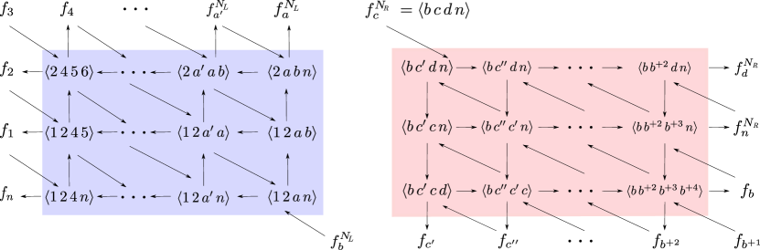
Figure 4. The initial seed $\Sigma_{0}$ for $\mathbb{C}[\widehat{\operatorname{Gr}}_{4,N_{L}}]\times\mathbb{C}[\widehat{\operatorname{Gr}}_{4,N_{R}}]$, which is a disjoint union of a seed $\Sigma_{0}^{L}$ for $\mathbb{C}[\widehat{\operatorname{Gr}}_{4,N_{L}}]$ (left) and a seed $\Sigma_{0}^{R}$ for $\mathbb{C}[\widehat{\operatorname{Gr}}_{4,N_{R}}]$ (right). We use the notation $x^{\prime}:=x-1,x^{\prime\prime}:=x-2$ and $x^{+i}:=x+i$. Mutable variables are in the shaded regions, the others are all frozen.

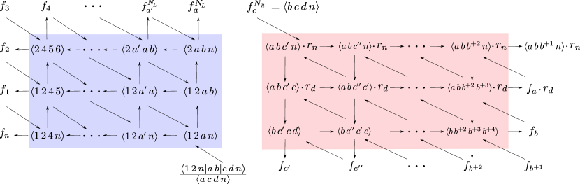
Figure 5. The result $\Psi(\Sigma_{0})$ of applying the product promotion to $\Sigma_{0}$. We use the notation $r_{x}:=\langle b\,c\,d\,n\rangle/\langle a\,b\,c\,x\rangle$ and $x^{\prime}:=x-1,x^{\prime\prime}:=x-2,x^{+i}:=x+i$.

Figure 6. The seed $\operatorname{Fr}(\Sigma_{1})=\operatorname{Fr}(\Sigma_{1}^{a,c})$ for $\mathbb{C}[\operatorname{Gr}_{4,n}]$. $\operatorname{Fr}(\Sigma_{1})$ is obtained from $\Sigma_{1}$ by freezing the variables in the dashed boxes. We use the notation $x^{\prime}:=x-1$ and $x^{+i}:=x+i$.

Proof of Theorem 4.7.

Let $\Sigma_{0}$ denote the initial seed for $\mathbb{C}[\widehat{\operatorname{Gr}}^{\circ}_{4,N_{L}}]\times\mathbb{C}[\widehat{\operatorname{Gr}}^{\circ}_{4,N_{R}}]$ shown in Figure 4. We note that $\Sigma_{0}$ is indeed a seed because each connected component is a cyclic shift of the rectangles seed for $\mathbb{C}[\widehat{\operatorname{Gr}}^{\circ}_{4,N_{L}}]$ and $\mathbb{C}[\widehat{\operatorname{Gr}}^{\circ}_{4,N_{R}}]$. If we apply product promotion to $\Sigma_{0}$, we obtain the “promoted seed” $\Psi(\Sigma_{0})$, shown in Figure 5.

Next we claim that the seed $\Sigma_{1}$ shown in Figure 6 is a seed for $\mathbb{C}[\operatorname{Gr}_{4,n}^{\circ}]$. To prove this, note that in $\mathbb{C}[\operatorname{Gr}_{4,n}^{\circ}]$, we have

(18) $$\langle c\,d\,n\,|\,a\,b\,|\,n\,1\,2\rangle\langle 1\,a\,d\,n\rangle=\langle 1\,2\,d\,n\rangle\langle 1\,a\,b\,n\rangle\langle a\,c\,d\,n\rangle+\langle 1\,2\,a\,n\rangle\langle 1\,c\,d\,n\rangle\langle a\,b\,d\,n\rangle.$$

So to prove that $\Sigma_{1}$ is a seed for $\mathbb{C}[\operatorname{Gr}_{4,n}^{\circ}]$, it suffices to show that the seed $\Sigma^{\prime}_{1}$ obtained from $\Sigma_{1}$ by mutating at $\langle c\,d\,n\,|\,a\,b\,|\,n\,1\,2\rangle$ is a seed for $\mathbb{C}[\operatorname{Gr}_{4,n}^{\circ}]$.

Figure 7. The plabic graph for $\operatorname{Gr}_{4,n}$ whose corresponding seed is $\Sigma_{1}^{\prime}$ in the proof of Theorem 9.1. We use the notation $x^{\prime}:=x-1,x^{\prime\prime}:=x-2$ and $x^{+i}:=x+i$. Mutating at the face $\langle 1\,a\,d\,n\rangle$ (dashed circle) gives the seed $\Sigma_{1}$.

Since all cluster and frozen variables of $\Sigma^{\prime}_{1}$ are Plücker coordinates, we can verify that $\Sigma^{\prime}_{1}$ is a seed for $\mathbb{C}[\operatorname{Gr}_{4,n}^{\circ}]$ by constructing a reduced plabic graph $G$ whose target-labeled seed is $\Sigma^{\prime}_{1}$. Such a reduced plabic graph is shown in Figure 7.

Now let $\operatorname{Fr}(\Sigma_{1})$ be the seed obtained from $\Sigma_{1}$ by freezing the cluster variables $\langle 1\,2\,n\,|\,a\,b\,|\,c\,d\,n\rangle$, $\langle 1\,a\,b\,n\rangle$, $\langle a-1\,a\,b\,n\rangle$, $\langle a\,b\,d\,n\rangle$, $\langle a\,b\,b+1\,n\rangle$, $\langle a\,b\,c\,n\rangle$, $\langle a\,b\,c\,d\rangle$, $\langle b\,c\,d\,n\rangle$, and $\langle a\,c\,d\,n\rangle$ (see Figure 6).

We will show that the product promotion, viewed as a map $\Psi:\mathcal{A}(\Sigma_{0})\to\mathcal{A}(\operatorname{Fr}(\Sigma_{1}))$, is a quasi-homomorphism of cluster algebras. More specifically, we will show that the two seeds $\Sigma_{0}$ and $\operatorname{Fr}(\Sigma_{1})$ satisfy the conditions of Definition 3.23. These two seeds are shown in Figures 4 and 6.

Looking at Figure 5 and Figure 6, we see immediately that conditions (1) and (3) of Definition 3.23 hold: the images $\Psi(x_{i})$ of mutable variables (shown in Figure 5) differ from their counterparts (shown in Figure 6), only by the frozen variables $\{\langle a\,b\,c\,n\rangle,\langle a\,b\,c\,d\rangle,\langle b\,c\,d\,n\rangle\}.$ The induced subquivers obtained by restricting to the mutable cluster variables agree.

Condition (2), that the corresponding exchange ratios agree, holds for the mutable variables in the left “$N_{L}$” connected component of $\Psi(\Sigma_{0})$. Indeed, this holds by inspection for $\langle 12an\rangle$, and the neighborhoods of all other mutable variables are identical in the two seeds.

We now show condition (2) holds for the remaining exchange ratios. We first consider the leftmost column of mutable cluster variables from the “$N_{R}$” connected component of $\Psi(\Sigma_{0})$ and the corresponding ones in $\operatorname{Fr}(\Sigma_{1})$. We have:

$$\hat{y}_{\Psi(\Sigma_{0})}\left(\langle a\,b\,c^{\prime}\,n\rangle\cdot r_{n}\right) =\hat{y}_{\operatorname{Fr}(\Sigma_{1})}\left(\langle a\,b\,c^{\prime}\,n\rangle\right)=\frac{\langle a\,b\,c^{\prime\prime}\,n\rangle\langle a\,b\,c^{\prime}\,c\rangle}{\langle a\,b\,c\,n\rangle\langle a\,b\,c^{\prime\prime}\,c^{\prime}\rangle}$$

$$\hat{y}_{\Psi(\Sigma_{0})}\left(\langle a\,b\,c^{\prime}\,c\rangle\cdot r_{d}\right) =\hat{y}_{\operatorname{Fr}(\Sigma_{1})}\left(\langle a\,b\,c^{\prime}\,c\rangle\right)=\frac{\langle a\,b\,c^{\prime\prime}\,c^{\prime}\rangle\langle b\,c^{\prime}\,c\,d\rangle\langle a\,b\,c\,n\rangle}{\langle b\,c^{\prime\prime}\,c^{\prime}\,c\rangle\langle a\,b\,c^{\prime}\,n\rangle\langle a\,b\,c\,d\rangle}$$

$$\hat{y}_{\Psi(\Sigma_{0})}\left(\langle b\,c^{\prime}\,c\,d\rangle\right) =\hat{y}_{\operatorname{Fr}(\Sigma_{1})}\left(\langle b\,c^{\prime}\,c\,d\rangle\right)=\frac{\langle b\,c^{\prime\prime}\,c^{\prime}\,c\rangle\langle a\,b\,c\,d\rangle f_{c^{\prime}}}{\langle a\,b\,c^{\prime}\,c\rangle\langle b\,c\,d\,n\rangle f_{c^{\prime\prime}}}$$

We now consider the exchange ratios for the other cluster variables. The cluster variables of the first and second rows (in the $N_{R}$ part) of $\Psi(\Sigma_{0})$ differ from the cluster variables of the corresponding rows of $\operatorname{Fr}(\Sigma_{1})$ just by common factors ($r_{n}$ and $r_{d}$ respectively). Moreover, for each cluster variable $x_{i}$ in $\Psi(\Sigma_{0})$ not in its first column, the number of out-going arrows $i\rightarrow j$ such that $x_{j}$ is in row $r$ equals the number of in-going arrows $l\rightarrow i$ with $x_{l}$ from the same row $r$. Therefore, any common factor among the row $r$ cancels in $\hat{y}(x_{i})$. Hence $\Psi(\Sigma_{0})$ and $\operatorname{Fr}(\Sigma_{1})$ have the same exchange ratios.

Therefore we have a quasi-homomorphism of cluster algebras $\Psi:\mathcal{A}(\Sigma_{0})\to\mathcal{A}(\operatorname{Fr}(\Sigma_{1}))$, where $\mathcal{A}(\operatorname{Fr}(\Sigma_{1}))$ is a subcluster algebra of $\mathbb{C}[\operatorname{Gr}_{4,n}^{\circ}]$, in the sense of [FWZd, Definition 4.2.6]. But then by definition of quasi-homomorphism, if we promote a cluster variable (respectively, cluster) of $\mathbb{C}[\widehat{\operatorname{Gr}}_{4,N_{L}}^{\circ}]\times\mathbb{C}[\widehat{\operatorname{Gr}}_{4,N_{R}}^{\circ}]$, we obtain a cluster variable (respectively, cluster) of $\mathcal{A}(\operatorname{Fr}(\Sigma_{1}))$, up to multiplication by Laurent monomials in the frozen variables of $\mathcal{A}(\operatorname{Fr}(\Sigma_{1}))$.

The final claim we need to prove is that if we promote a cluster variable of $\mathbb{C}[\widehat{\operatorname{Gr}}_{4,N_{L}}^{\circ}]\times\mathbb{C}[\widehat{\operatorname{Gr}}^{\circ}_{4,N_{R}}]$, we obtain a cluster variable of $\mathbb{C}[\operatorname{Gr}_{4,n}^{\circ}]$, up to multiplication by a Laurent monomial in the set $\mathcal{T^{\prime}}$. To show this, we consider 2 slight modifications of $\Psi(\Sigma_{0})$ and $\operatorname{Fr}(\Sigma_{1})$.

Figure 8. To construct the seed $\Lambda$ from $\Psi(\Sigma_{0})$, add the variables $f_{c}=\langle 1cdn\rangle,f_{d}=\langle 12dn\rangle,\langle abdn\rangle,\langle abcn\rangle,\langle abcd\rangle,\langle acdn\rangle$, then the dashed purple and dotted red arrows. The purple dashed arrows are all present in $\Omega$, while the red dotted arrows make the exchange ratios of the mutable variables of $\Lambda$ match up with those in $\Omega$. The frozen variables of $\Lambda$ are boxed.

Let $\Omega$ be the seed obtained from $\operatorname{Fr}(\Sigma_{1})$ by unfreezing all its frozen variables which are not in $\mathcal{T}^{\prime}$. Let $\Lambda$ be the seed obtained from $\Psi(\Sigma_{0})$ by:

• adding the variables $f_{c}=\langle 1cdn\rangle,f_{d}=\langle 12dn\rangle,\langle abdn\rangle,\langle abcn\rangle,\langle abcd\rangle,\langle acdn\rangle$;

• freezing all variables in $\mathcal{T}^{\prime}$ and declaring all other variables mutable;

• adding the purple dashed arrows shown in Figure 8;

• and then finally adding the red dotted arrows between elements of $\mathcal{T^{\prime}}$ and mutable variables so that all the newly mutable variables have the same exchange ratios as the corresponding newly mutable variables in $\Omega$.

Notice that we did not add any arrow incident to a mutable variable of $\Psi(\Sigma_{0})$, so we did not affect any of the exchange ratios that we previously analyzed. The final step of adding the red dotted arrows is possible because after we added the purple dashed arrows in Figure 8, the exchange ratios for newly mutable variables (those which were not mutable in $\Psi(\Sigma_{0})$) differ from the exchange ratios in $\Omega$ by Laurent monomials in $\mathcal{T}^{\prime}$.

We’ve now constructed two cluster algebras $\mathcal{A}(\Lambda)$ and $\mathcal{A}(\Omega)$ whose cluster variables are in bijection, and whose frozen variables are precisely $\mathcal{T^{\prime}}$. Moreover, each initial cluster variable of $\mathcal{A}(\Lambda)$ is proportional to the corresponding cluster variable of $\mathcal{A}(\Omega)$, and the exchange ratios around corresponding initial cluster variables agree. These properties are preserved under mutation, so each cluster variable of $\mathcal{A}(\Lambda)$ is proportional to the corresponding cluster variable of $\mathcal{A}(\Omega)$, with frozen factor a Laurent monomial in $\mathcal{T^{\prime}}$. The cluster variables of $\mathcal{A}(\Psi(\Sigma_{0}))$ are cluster variables of $\mathcal{A}(\Lambda)$ because the variables we added to $\Lambda$ are adjacent only to variables which are frozen in $\Psi(\Sigma_{0})$. Similarly, cluster variables of $\mathcal{A}(\operatorname{Fr}(\Sigma_{1}))$ are cluster variables of $\mathcal{A}(\Omega)$, since the seeds only differ by freezing. So the frozen factors of variables in $\mathcal{A}(\Psi(\Sigma_{0}))$ are Laurent monomials in $\mathcal{T^{\prime}}$. ∎

As a consequence of Definition 4.2 and Theorem 4.7, we obtain the following.

Corollary 4.10.

The polynomial ${\langle i\,j\,n\,|\,a\,b\,|\,c\,d\,n\rangle}={\langle a\,b\,n\,|\,c\,d\,|\,i\,j\,n\rangle}={\langle c\,d\,n\,|\,i\,j\,|\,a\,b\,n\rangle}$ is a cluster variable and hence positive on $\operatorname{Gr}^{>0}_{4,n}$ whenever $i<j<a<b<c<d<n$. And the polynomial ${\langle i\,j\,\ell\,|\,b\,a\,|\,c\,d\,n\rangle}$ is a cluster variable and hence positive on $\operatorname{Gr}^{>0}_{4,n}$ whenever

• $i<j<\ell<a<b<c<d<n$ or

• $c<d<i<j<\ell<a<b<n$ or

• $a<b<i<j<\ell<c<d<n$.

Remark 4.11.

Note that if $\{i,j,\ell,q,r,s,t\}\subset\{1,2,3,\dots,a-1,n\}$, we have that

$$\Psi(\langle i\,j\,\ell\,|\,r\,q\,|\,s\,t\,b\rangle)=\frac{\langle i\,j\,\ell\,|\,r\,q\,|\,s\,t\,|\,b\,a\,|\,c\,d\,n\rangle}{\langle a\,c\,d\,n\rangle}.$$

Therefore we can extend Corollary 4.10 to higher degree chain polynomials, and conclude e.g. that if $i<j<\ell<q<r<s<t<b$, then $\langle i\,j\,\ell\,|\,r\,q|s\,t\,|\,b\,a\,|\,c\,d\,n\rangle=\langle i\,j\,\ell\,|\,q\,r|s\,t\,|\,a\,b\,|\,c\,d\,n\rangle$ is a cluster variable and hence positive on $\operatorname{Gr}^{>0}_{4,n}$.

Figure 9. Left: the seed $\operatorname{Fr}(\Sigma_{1})$ in the case of upper promotion, where $a=1$ and $b=2$. Right: the seed $\operatorname{Fr}(\Sigma_{1})$ when $a=2$ and $b=3$. We use the notation $x^{\prime}:=x-1$ and $x^{+i}:=x+i$.

4.3. Degenerate cases of Theorem 4.7

There are a few special cases of Theorem 4.7 that warrant discussion. The proofs are all analogous to those of Theorem 4.7 so we omit them.

• Theorem 4.7 holds also for upper promotion (c.f. Definition 4.4), where

  $$\mathcal{T}=\mathcal{T^{\prime}}=\{\langle abcn\rangle,\langle abcd\rangle,\langle bcdn\rangle\}.$$

  In this case, $\Sigma_{0}$ and $\Psi(\Sigma_{0})$ consist only of the right connected component of the quiver in Figures 4 and 5; the seed $\operatorname{Fr}(\Sigma_{1})$ is shown on the left in Figure 9.

• If $a=2$, then Theorem 4.7 holds for $\mathcal{T}=\{\langle abdn\rangle,\langle abcn\rangle,\langle abcd\rangle,\langle bcdn\rangle,\langle acdn\rangle,\langle a\,b\,b+1\,n\rangle\}$ and $\mathcal{T^{\prime}}=\{\langle abcn\rangle,\langle abcd\rangle,\langle bcdn\rangle\}$. In this case, the left connected component of $\Sigma_{0}$ and $\Psi(\Sigma_{0})$ consist of the single frozen variable $\langle 123n\rangle$; the seed $\operatorname{Fr}(\Sigma_{1})$ is shown on the right in Figure 9.

• If $a=3$ or $c=b+1$, then some of the Plücker coordinates in Figure 6 coincide. If $a=3$, then $\langle 2abn\rangle=\langle a-1\,a\,b\,n\rangle$; if $c=b+1$ then $\langle abcn\rangle=\langle a\,b\,b+1\,n\rangle$. To obtain the quiver for $\operatorname{Fr}(\Sigma_{1})$ in these cases, one should identify the vertices labeled by equal Plücker coordinates.

5. The BCFW map and the BCFW product

In this section we define the BCFW map on nonnegative Grassmannians, and define the closely related BCFW product on positroid cells in terms of plabic graphs. We will use these to define BCFW cells in Section 10. We will later see that the BCFW product is closely related to product promotion (see for example Definition 7.1, Theorem 7.15, and Theorem 11.3.)

Notation 5.1.

Fix $1\leq a<b<c<d<n$ such that $a,b$ and $c,d,n$ are consecutive, and let $N_{L}=\{1,\dots,a,b,n\}$ and $N_{R}=\{b,\dots,c,d,n\}$, as in 4.1. Also fix $k\leq n$ and two nonnegative integers $k_{L}\leq|N_{L}|$ and $k_{R}\leq|N_{R}|$ such that $k_{L}+k_{R}+1=k$.

Definition 5.2 (BCFW Map).

Using 5.1, the BCFW map is the rational map

$$\iota_{\bowtie}\;:\;{\operatorname{Gr}}^{\scriptscriptstyle\geq 0}_{k_{L},N_{L}}\times\;\operatorname{Gr}_{1,5}^{\scriptscriptstyle>0}\;\times\;{\operatorname{Gr}}^{\scriptscriptstyle\geq 0}_{k_{R},N_{R}}\;\dashrightarrow\;\operatorname{Gr}_{k,n}^{\scriptscriptstyle\geq 0}$$

where $(A,[\alpha:\beta:\gamma:\delta:\varepsilon],B)$ is mapped to the (row span of the) $k\times n$ matrix $(*)$ in Figure 10. Here $[\alpha:\beta:\gamma:\delta:\varepsilon]$ denote the positive homogeneous coordinates of a point in $\operatorname{Gr}_{1,5}^{>0}\subset\mathbb{R}\mathbb{P}^{4}$.

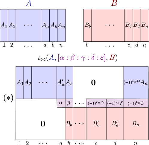
Figure 10. The image of $(A,[\alpha:\beta:\gamma:\delta:\varepsilon],B)$ under the BCFW map $\iota_{\bowtie}$. Here, $A^{\prime}_{a}:=A_{a}+\frac{\alpha}{\beta}A_{b}$, $B_{d}^{\prime}:=B_{d}+\frac{\delta}{\varepsilon}B_{n}$, $B_{c}^{\prime}:=B_{c}+\frac{\gamma}{\delta}B_{d}^{\prime}$, and in a standard abuse of notation we identify the matrix $(*)$ with its rowspan.

Remark 5.3.

1. The definition of the BCFW map $\iota_{\bowtie}$ depends on the choices of $a,c,n$, etc. in 5.1. Such choice will always be fixed in advance and, if it is clear, we will not mention it.

2. The rowspan of $(*)$ depends only on the values of $\alpha,\beta,\gamma,\delta,\varepsilon$ up to simultaneous rescaling. Similarly, it only depends on the rowspans of $A$ and $B$ rather than the specific matrices. Additionally, for generic inputs the rank of $(*)$ is $k$. Therefore the map $\iota_{\bowtie}$ is well defined.

3. The numbers $k_{L}$ or $k_{R}$ may be zero. If e.g. $k_{L}=0$ then $\operatorname{Gr}_{k_{L},N_{L}}$ is a point and $A$ is a $0\times(a+2)$ matrix. The matrix $(*)$ is $(k_{R}+1)\times n$ and the columns $1,\dots,a-1$ are zero columns.

4. In the special case that $k_{L}=0$ and $a=1$, and hence $N_{L}=\{a,b,n\}$, we call $\iota_{\bowtie}$ the upper BCFW map. We omit the first argument and write

   $$\iota_{\bowtie}\;:\;\operatorname{Gr}_{1,5}^{\scriptscriptstyle>0}\;\times\;{\operatorname{Gr}}^{\scriptscriptstyle\geq 0}_{k_{R},N_{R}}\;\dashrightarrow\;\operatorname{Gr}_{k,n}^{\scriptscriptstyle\geq 0}.$$

5. For any set of indices $N\subset[n]$ ordered according to the usual order on integers, the definition of $\iota_{\bowtie}$ naturally extends to the setting of $\operatorname{Gr}_{k,N}^{\scriptscriptstyle\geq 0}$ rather than $\operatorname{Gr}_{k,n}^{\scriptscriptstyle\geq 0}$. We replace $1$ and $n$ in the definition with the smallest and largest elements of $N$, respectively.

We now introduce an operation on positroid cells we call BCFW product, fixing notation as in 5.1. We will define the operation in terms of plabic graphs, see Appendix A.

Definition 5.4 (BCFW product).

Let $G_{L},G_{R}$ be plabic graphs of respective ranks $k_{L},k_{R}$ on $N_{L},N_{R}$ as in 5.1, let $\mathcal{P}_{L},\mathcal{P}_{R}$ be their corresponding positroids and $S_{L},S_{R}$ their corresponding positroid cells. The BCFW product of $G_{L}$ and $G_{R}$, denoted $G_{L}\bowtie G_{R}$, is the plabic graph in the right-hand side of Figure 11. We also denote by $\mathcal{P}_{L}\bowtie\mathcal{P}_{R}$ and $S_{L}\bowtie S_{R}$ the positroid and positroid cell corresponding to $G_{L}\bowtie G_{R}$, and we call these the BCFW products of $\mathcal{P}_{L},\mathcal{P}_{R}$ and $S_{L},S_{R}$.

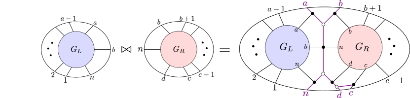
Figure 11. The BCFW product $G_{L}\bowtie G_{R}$ of plabic graphs $G_{L}$ and $G_{R}$.

The notation $\bowtie$ is intended to echo the “butterfly” connecting $G_{L},G_{R}$ in the right-hand side of Figure 11. While we overload this notation, it will always be clear from context what kind of object it denotes. Note that whenever we apply a BCFW product, we will assume that the cells $S_{L}$ and $S_{R}$ use index sets $N_{L}$ and $N_{R}$ as in 5.1.

We will show the BCFW map on a pair of positroid cells gives their BCFW product, under appropriate assumptions. First, we need a definition.

Definition 5.5.

Let $V\in\operatorname{Gr}_{k,N}$. A subset $J\subseteq N$ is coindependent for $V$ if $V$ has a nonzero Plücker coordinate $\langle I\rangle_{V}$, such that $I\cap J=\emptyset$. By convention, if $k=0$ then all subsets are coindependent for $V$. If $S\subset\operatorname{Gr}_{k,n}$, then $J$ is coindependent for $S$ if $J$ is coindependent for all $V\in S$.

Remark 5.6.

By Proposition A.7 and Theorem A.10, $J$ is coindependent for a cell $S$ if and only if every plabic graph $G$ for $S$ has a perfect orientation where all boundary vertices in $J$ are sinks.

Notation 5.7 (Coindependence).

We use 5.1 and fix positroid cells $S_{L}\subset{\operatorname{Gr}}^{\geq 0}_{k_{L},N_{L}}$ and $S_{R}\subset{\operatorname{Gr}}^{\geq 0}_{k_{R},N_{R}}$ such that $\{a,b,n\}$ is coindependent for $S_{L}$ and $\{b,c,d,n\}$ is coindependent for $S_{R}$.

We will prove Proposition 5.8 (1) below, and defer the proof of (2) to Proposition 10.2.

Proposition 5.8.

Fix $S_{L},S_{R}$ as in 5.7. Then we have the following:

1. The map $\iota_{\bowtie}$ is well-defined on $S_{L}~{}\times~{}\operatorname{Gr}_{1,5}^{\scriptscriptstyle>0}~{}\times~{}S_{R}$ and its image is $S_{L}\bowtie S_{R}.$

2. The map $\iota_{\bowtie}$ is injective on $S_{L}~{}\times~{}\operatorname{Gr}_{1,5}^{\scriptscriptstyle>0}~{}\times~{}S_{R}$, and hence we have an isomorphism

   $$\iota_{\bowtie}:S_{L}\times\operatorname{Gr}_{1,5}^{\scriptscriptstyle>0}\times S_{R}\;\xrightarrow{\sim}\;S_{L}\bowtie S_{R}.$$

It follows that $\dim(S_{L}\bowtie S_{R})=\dim S_{L}+\dim S_{R}+4$.

We note that when $k_{L}=0$ and $a=1$ above, $\{a,b,n\}$ is coindependent for $S_{L}$, so this proposition covers the case that $\iota_{\bowtie}$ is the upper BCFW map.

Proof.

We first show that $\iota_{\bowtie}$ is well-defined on $S_{L}\times\operatorname{Gr}_{1,5}^{\scriptscriptstyle>0}\times S_{R}$ and that the image is $S_{L}\bowtie S_{R}$.

Choose reduced plabic graphs $G_{L},G_{R}$ for $S_{L},S_{R}$. The coindependence assumption plus Remark 5.6 implies that $G_{L}$, respectively $G_{R}$, has a perfect orientation $\mathcal{O}_{L}$, respectively $\mathcal{O}_{R}$, where $\{a,b,n\}$, respectively $\{b,c,d,n\}$, are sinks. We may assume that both $\mathcal{O}_{L}$ and $\mathcal{O}_{R}$ are acyclic using the coindependence assumption and Lemma A.8. Now, orient the edges of $G_{L}\bowtie G_{R}$ according to $\mathcal{O}_{L}$, $\mathcal{O}_{R}$ and orient all other edges according to Figure 12.

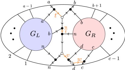
Figure 12. The perfect orientation and edge weighting of $G_{L}\bowtie G_{R}$ used in the proof of Proposition 5.8. All weights are positive, and edge weights of 1 are omitted.

This gives a perfect orientation of $G_{L}\bowtie G_{R}$ whose sources are $a$ together with the sources of $\mathcal{O}_{L}$ and $\mathcal{O}_{R}$. Thus $S_{L}\bowtie S_{R}$ is rank $k=1+k_{L}+k_{R}$.

Now, we will analyze the path matrix of $G_{L}\bowtie G_{R}$ (cf Definition A.9) and show that one can perform invertible row operations to obtain precisely the matrix $(*)$ of Figure 10. First, by using gauge transformations (cf Lemma A.11) of the $10$ internal black/white vertices shown in Figure 12, as well as the seven internal vertices of $G_{L}$ and $G_{R}$ which are incident to the boundary vertices $\{a,b,n\}$ of $G_{L}$ and $\{b,c,d,n\}$ of $G_{R}$, we can assume that the $21$ oriented edges in Figure 12 are weighted as in the figure, where edge weights of $1$ are omitted.

Now, let $A,B$ be path matrices of $G_{L},G_{R}$ with respect to the perfect orientations $\mathcal{O}_{L},\mathcal{O}_{R}$. Note that $A,B$ represent elements of $S_{L},S_{R}$. By inspection of the paths in Figure 12, the path matrix of $G_{L}\bowtie G_{R}$ is

$$\setcounter{MaxMatrixCols}{11}\begin{bmatrix}A_{1}&\cdots&A_{a-1}&0&-tA_{a}&0&\cdots&0&(-1)^{k_{R}+1}uvwA_{a}^{\prime}&(-1)^{k_{R}+1}uvA_{a}^{\prime}&(-1)^{k_{R}+1}A_{n}^{\prime}\\ 0&\cdots&0&1&t&0&\cdots&0&(-1)^{k_{R}}uvw&(-1)^{k_{R}}uv&(-1)^{k_{R}}u\\ 0&\cdots&\cdots&0&B_{b}&B_{b+1}&\cdots&B_{c-1}&B_{c}^{\prime}&B_{d}^{\prime}&B_{n}\\ \end{bmatrix}$$

where

$$A^{\prime}_{a}:=A_{a}+\tfrac{1}{t}A_{b},\;\;\;B_{d}^{\prime}:=B_{d}+vB_{n},\;\;\;B_{c}^{\prime}:=B_{c}+wB_{d}^{\prime},\;\;\;A_{n}^{\prime}=A_{n}+uA_{a}^{\prime},$$

and the “middle” row is indexed by the source $a$. By adding a suitable multiple of the row indexed by $a$ to the rows above, one obtains a full-rank matrix of the form

(19) $$\setcounter{MaxMatrixCols}{11}\begin{bmatrix}A_{1}&\cdots&A_{a-1}&A_{a}^{\prime}&A_{b}&0&\cdots&0&0&0&(-1)^{k_{R}+1}A_{n}\\ 0&\cdots&0&1&t&0&\cdots&0&(-1)^{k_{R}}uvw&(-1)^{k_{R}}uv&(-1)^{k_{R}}u\\ 0&\cdots&\cdots&0&B_{b}&B_{b+1}&\cdots&B_{c-1}&B_{c}^{\prime}&B_{d}^{\prime}&B_{n}\\ \end{bmatrix}.$$

Setting $t=\frac{\beta}{\alpha},u=\frac{\varepsilon}{\alpha},v=\frac{\delta}{\varepsilon},w=\frac{\gamma}{\delta}$ and rescaling the row indexed by $a$ by $\alpha$ in (19) gives a full-rank matrix exactly of the form $(*)$ in Figure 10. Thus, $\iota_{\bowtie}$ is well-defined on $(A,[\alpha:\beta:\gamma:\delta:\varepsilon],B)$ and $\iota_{\bowtie}$ sends this triple to the rowspan of the matrix in (19) with the variable substitutions mentioned above. The rowspan of (19) lies in $S_{L}\bowtie S_{R}$ for any positive parameter values. This shows that $\iota_{\bowtie}$ is well-defined on $S_{L}\times\operatorname{Gr}_{1,5}^{>0}\times S_{R}$ and that $\iota_{\bowtie}(S_{L}\times\operatorname{Gr}_{1,5}^{>0}\times S_{R})\subset S_{L}\bowtie S_{R}$. To see the reverse inclusion, note that varying $[\alpha:\beta:\delta:\gamma:\varepsilon]$ and the values of the weights in $A,B$ is the same as varying the values of the weights on $G_{L}\bowtie G_{R}$, and so the matrices in (19) will vary over all points in $S_{L}\bowtie S_{R}$.

The statement that $\iota_{\bowtie}$ is injective on $S_{L}\times\operatorname{Gr}_{1,5}^{>0}\times S_{R}$ is Proposition 10.2.

The dimension of $S_{L}\times\operatorname{Gr}_{1,5}^{>0}\times S_{R}$ is $\dim S_{L}+\dim S_{R}+4$ and $S_{L}\bowtie S_{R}$ is the image of this set under a bijective map, so has the same dimension. ∎

Remark 5.9 (BCFW map and product in physics).

An analogous matrix representation of the BCFW map $\iota_{\bowtie}$ (as in Figure 10) appeared in [Bou10, Equation (3.6)]. The first appearance of the “butterfly” plabic graph from Figure 11 is in [BH15, Equation (3.3)]. Note that the “butterfly” plabic graph $G_{L}\bowtie G_{R}$ is related to the BCFW bridge recurrence in momentum space (see [AHBC⁺16, Equation (2.26)]) by two applications of the inverse T-duality operation on plabic graphs (see [PSBW23, Definition 8.7, Remark 8.9]). See Figure 13 for an illustration.

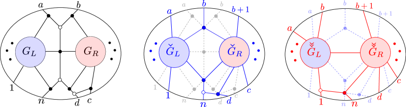
Figure 13. Applying inverse T-duality twice to $G_{L}\bowtie G_{R}$ gives the BCFW bridge recurrence in ‘momentum space’ [AHBC⁺16, Equation (2.26)]. We use the notation $\check{G}$ for the inverse T-dual of $G$. Left: $G_{L}\bowtie G_{R}$; center: application of inverse T duality to $G_{L}\bowtie G_{R}$; right: application of inverse T duality twice to $G_{L}\bowtie G_{R}$.

6. Standard and general BCFW cells

In this section we define the standard and general BCFW cells. We then introduce chord diagrams (cf. Definition 6.7) and recipes (cf. Definition 6.16), which label standard and general BCFW cells respectively. Finally, we define the BCFW matrix for each BCFW cell, a convenient representative matrix, and use it to show that BCFW cells in $\operatorname{Gr}_{k,n}^{\scriptscriptstyle\geq 0}$ are $4k$-dimensional.

First, we define BCFW cells. Recall the dihedral group action on $\operatorname{Gr}_{k,n}^{\scriptscriptstyle\geq 0}$ from Definition 2.3. We refer to the following collection of cells as general BCFW cells, or simply as BCFW cells.

Definition 6.1 (General BCFW cells).

The set of general BCFW cells is defined recursively:

1. For $k=0$, the trivial cell $\operatorname{Gr}^{\scriptscriptstyle>0}_{0,n}$ is a general BCFW cell.

2. If $S$ is a general BCFW cell, then so is any cell obtained by inserting a zero column.

3. If $S$ is a general BCFW cell, then so is any cyclic shift or reflection of $S$.

4. Fix the quantities in 5.1. If $S_{L}$ and $S_{R}$ are general BCFW cells on $N_{L}$ and $N_{R}$, then so is their BCFW product $S_{L}\bowtie S_{R}$.

Remark 6.2.

By Corollary 10.7, general BCFW cells satisfy the coindependence assumptions of Proposition 5.8. Thus, taking the BCFW product of two BCFW cells is the same as applying the BCFW map to them. So the “(Product)” step in Definition 6.1 could be equivalently stated as: if $S_{L}$ and $S_{R}$ are general BCFW cells, then so is $\iota_{\bowtie}(S_{L}\times\operatorname{Gr}_{1,5}^{\scriptscriptstyle>0}\times S_{R})$.

The standard BCFW cells, which we define below, are a particularly nice subset of BCFW cells. The images of the standard BCFW cells yield a tiling of the amplituhedron [ELT21].

Definition 6.3 (Standard BCFW cells).

Standard BCFW cells are defined recursively as follows.

1. For $k=0$, the trivial cell $\operatorname{Gr}_{0,n}$ is a standard BCFW cell.

2. If $S$ is a standard BCFW cell, then so is the cell obtained by inserting a zero column in the penultimate position.

3. Fix 5.1. If $S_{L}$ and $S_{R}$ are standard BCFW cells on $N_{L}$ and $N_{R}$, then their BCFW product $S_{L}\bowtie S_{R}$ is a standard BCFW cell.

Remark 6.4.

The standard BCFW cells defined here are the same as those in [KWZ20, ELT21], though Definition 6.3 uses different terminology than those two papers. Indeed, [KWZ20] obtains standard BCFW cells by applying the “BCFW bridge recurrence in momentum space”(see Figure 13, right), then applying T-duality twice. This is the same as repeatedly applying the BCFW product. [KWZ20] also gives an explicit construction of standard BCFW cells in terms of pairs of noncrossing lattice paths, while [ELT21] gives an explicit construction of standard BCFW cells in terms of chord diagrams, and shows that the two constructions agree [ELT21, Proposition 2.28].

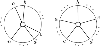
Figure 14. Standard BCFW cells (left) and general BCFW cells (right) in $\operatorname{Gr}^{\scriptscriptstyle\geq 0}_{1,n}$, where the $\ldots$ denote black lollipops in the remaining indices.

Example 6.5.

For $k=1$, the BCFW cells in $\operatorname{Gr}_{1,n}^{\scriptscriptstyle\geq 0}$ are indexed by the elements of $\binom{\scriptscriptstyle[n]}{5}$. For $I=\{a,b,c,d,e\}\in\binom{\scriptscriptstyle[n]}{5}$, the corresponding BCFW cell consists of points with Plücker coordinates $\langle a\rangle,\langle b\rangle,\langle c\rangle,\langle d\rangle,\langle e\rangle>0$ and all others zero. The plabic graph has a 5-valent white vertex adjacent to boundary vertices $a,b,c,d,e$ and all other vertices are black lollipops, see Figure 14. The standard BCFW cells for $k=1$ are only those where $a,b$ and $c,d$ are consecutive and $e=n$. For $k=n-4$, the totally positive Grassmannian $\operatorname{Gr}_{n-4,n}^{\scriptscriptstyle>0}$ is the only BCFW cell. It can be obtained from the point $\operatorname{Gr}_{0,4}^{>0}$ by repeatedly applying the upper BCFW map.

Remark 6.6.

It follows from the above definition that if $k>0$ then $k\leq n-4$ for a BCFW cell in $\operatorname{Gr}_{k,n}^{\scriptscriptstyle\geq 0}$. Hence, when one generates a BCFW cell with the (Product) step, $k_{R}\leq|N_{R}|-4$ and $k_{L}\leq\max(0,|N_{L}|-4)$. In terms of 5.1, $k_{L}\leq a-2$ and $k_{R}\leq c-b-1$, with the additional possibility that $k_{L}=0$ and $a=1$, which is the case of the upper BCFW map.

6.1. Standard BCFW cells from chord diagrams

In this section we introduce chord diagrams, and show how each gives an algorithm for constructing a standard BCFW cell. In Section 6.2 we then give a generalization of this algorithm, called a recipe, for constructing a general BCFW cell.

Definition 6.7 (Chord diagram [ELT21]).

Let $k,n\in\mathbb{N}$. A chord diagram $D\in\mathcal{CD}_{n,k}$ is a set of $k$ quadruples named chords, of integers in the set $\{1,\dots,n\}$ named markers, of the following form:

$$D\;=\;\{(a_{1},b_{1},c_{1},d_{1}),\dots,(a_{k},b_{k},c_{k},d_{k})\}\;\;\text{ where }\;\;b_{i}=a_{i}+1\text{ and }d_{i}=c_{i}+1$$

such that every chord $D_{i}=(a_{i},b_{i},c_{i},d_{i})\in D$ satisfies $1\;\leq\;a_{i}\;<\;b_{i}\;<\;c_{i}\;<\;d_{i}\;\leq\;n-1$ and no two chords $D_{i},D_{j}\in D$ satisfy $a_{i}\;=\;a_{j}$ or $a_{i}\;<\;a_{j}\;<\;c_{i}\;<\;c_{j}.$

It follows from this definition that the number of different chord diagrams with $n$ markers and $k$ chords is the Narayana number $N(n-3,k+1)$: $\left|\mathcal{CD}_{n,k}\right|\;=\;\frac{1}{k+1}\binom{n-4}{k}\binom{n-3}{k}$. As we explain in Definition 6.12 below, each chord diagram gives rise to a standard BCFW cell by encoding a sequence of BCFW products and penultimate zero column insertions.

$$D\;=\;\{(3,4,5,6),(5,6,8,9),(1,2,8,9),(10,11,12,13),(9,10,12,13),(8,9,13,14)\}$$

Figure 15. A chord diagram $D$ with $k=6$ chords $n=15$ markers.

See Figure 15, where we visualize such a chord diagram $D$ in the plane as a horizontal line with $n$ markers labeled $\{1,\dots,n\}$ from left to right, and $k$ nonintersecting chords above it, whose start and end lie in the segments $(a_{i},b_{i})$ and $(c_{i},d_{i})$ respectively. The definition imposes restrictions on the chords: they cannot start before $1$, end after $n-1$, or start or end on a marker. Two chords cannot start in the same segment $(s,s+1)$, and one chord cannot start and end in the same segment, nor in adjacent segments. Two chord cannot cross. Pictorially, the forbidden configurations are:

We say that a chord is a top chord if there is no chord above it, e.g. $D_{3}$ and $D_{6}$ in Figure 15. One natural way to label the chords is by $D_{1},\dots,D_{k}$ such that for all $1\leq j\leq k$, $D_{j}$ is the rightmost top chord among the set of chords $\{D_{1},\dots,D_{j}\}$ as in Figure 15. This is equivalent to sorting the chords according to their ends. The visualization of chord diagrams provides us with useful terminology, which we illustrate in Figure 15. This terminology will primarily be used in Section 8.

Definition 6.8 (Terminology for chords).

A chord is a top chord if there is no chord above it, and otherwise it is a descendant of the chords above it, called its ancestors, and in particular a child of the chord immediately above it, which is called its parent. For example, $D_{4}$ has parent $D_{5}$ and ancestors $D_{5}$ and $D_{6}$. Two chords are siblings if they are either top chords or children of a common parent; for example, $D_{1}$ and $D_{2}$ are siblings, and $D_{3}$ and $D_{6}$ are siblings. Two chords are same-end if their ends occur in a common segment $(e,e+1)$, are head-to-tail if the first ends in the segment where the second starts, and are sticky if their starts lie in consecutive segments $(s,s+1)$ and $(s+1,s+2)$. For example, chords $D_{2}$ and $D_{3}$ are same-end, chords $D_{1}$ and $D_{2}$ are head-to-tail, and chords $D_{5}$ and $D_{6}$ are sticky.

Remark 6.9.

The definition of a chord diagram naturally extends to general index sets with a total order. Thus, we will sometimes work with a finite set of markers $N\subset\{1,\dots,n\}$ rather than $\{1,\dots,n\}$, and a set $K$ of chord indices rather than $\{1,\dots,k\}$, and denote these diagrams by $\mathcal{CD}_{N,K}$. We will always have that the largest marker is $n\in N$, the starts and ends of chords will be consecutive pairs in $N$ (and also $\mathbb{N}$) and the rightmost top chord will be denoted by $D_{\operatorname{{\it k}}}=D_{\max K}$.

Definition 6.10 (Left and right subdiagrams).

Let $D$ be a chord diagram in $\mathcal{CD}_{N,K}$. A subdiagram is obtained by restricting to a subset of the chords and a subset of the markers which contains both these chords and the marker $n$. Let $D_{\operatorname{{\it k}}}=(a,b,c,d)$ be the rightmost top chord of $D$, where $1\leq a<b<c<d<n$, and moreover $a,b$ and $c,d$ are consecutive in $N$.

In the case that $d,n$ are consecutive as well we define $D_{L}$, the left subdiagram of $D$, on the markers $N_{L}=\{1,2,\dots,a,b,n\}$ and the right subdiagram $D_{R}$ on $N_{R}=\{b,\dots,c,d,n\}$. The subdiagram $D_{L}$ contains all chords that are to the left of $D_{\operatorname{{\it k}}}$, and $D_{R}$ contains the descendants of $D_{\operatorname{{\it k}}}$.

Example 6.11.

For the chord diagram $D$ in Figure 15, the rightmost top chord is $D_{6}=(8,9,13,14)$, so $N_{L}=\{1,\dots,9,15\}$ and $D_{L}=\{D_{1},D_{2},D_{3}\}$, while $N_{R}=\{9,\dots,15\}$ and $D_{R}=\{D_{4},D_{5}\}$.

Definition 6.12 (Standard BCFW cell from a chord diagram).

Let $D\in\mathcal{CD}_{N,K}$ be a chord diagram. We recursively construct from $D$ a standard BCFW cell $S_{D}$ in ${\operatorname{Gr}}^{\scriptscriptstyle\geq 0}_{K,N}$ as follows:

1. If $k=0$, then the BCFW cell is the trivial cell $S_{D}:=\operatorname{Gr}^{\scriptscriptstyle\geq 0}_{0,N}$.

2. Otherwise, let $D_{\operatorname{{\it k}}}=(a,b,c,d)$ be the rightmost top chord of $D$ and let $p$ denote the penultimate marker in $N$.

   1. If $d\neq p$, let $D^{\prime}$ be the subdiagram on $N\setminus\{p\}$ with the same chords as $D$, and let $S_{D^{\prime}}$ be the standard BCFW cell associated to $D^{\prime}$. Then, we define $S_{D}:=\operatorname{pre}_{p}S_{D^{\prime}}$, which denotes the standard BCFW cell obtained from $S_{D^{\prime}}$ by inserting a zero column in the penultimate position $p$.

   2. If $d=p$, let $S_{L}$ and $S_{R}$ be the standard BCFW cells on $N_{L}$ and $N_{R}$ associated to the left and right subdiagrams $D_{L}$ and $D_{R}$ of $D$. Then, we let $S_{D}:=S_{L}\bowtie S_{R}$, the standard BCFW cell which is their BCFW product as in Definition 5.4.

Figure 16. Recursive construction of a standard BCFW cell from a chord diagram as in Definition 6.12. Top left (right): construction of $D$ ($G_{D}$) from $D^{\prime}$ ($G^{\prime}$) as in $(1a)$; bottom left (right) construction of $D$ ($G_{D}$) from $D_{L},D_{R}$ ($G_{L},G_{R}$) as in $(1b)$.

Example 6.13.

The standard BCFW cell $S_{D}$ of the chord diagram $D$ in Figure 15 is $S_{L}\bowtie S_{R}$ where the chord subdiagrams $D_{L},D_{R}$ are as in Example 6.11. One can keep applying the recursive definition and obtain:

$$S_{L}\; =\;\operatorname{Gr}_{0,\{1,2,15\}}\bowtie\left(\left(\operatorname{Gr}_{0,\{2,3,4,15\}}\bowtie\operatorname{Gr}_{0,\{4,5,6,15\}}\right)\bowtie\operatorname{Gr}_{0,\{6,7,8,9,15\}}\right)$$

$$S_{R}\; =\;\operatorname{pre}_{14}\left(\operatorname{Gr}_{0,\{9,10,15\}}\bowtie\left(\operatorname{Gr}_{0,\{10,11,15\}}\bowtie\operatorname{Gr}_{0,\{11,12,13,15\}}\right)\right)$$

Remark 6.14.

It is not hard to see that every standard BCFW cell arises from a chord diagram. Moreover two distinct chord diagrams give rise to different cells [ELT21]. Therefore every standard BCFW cell arises from a unique chord diagram.

Remark 6.15.

In Definition 6.12 we have taken care to work with chord diagrams on general index sets $N$, but in what follows we often slightly abuse notation and consider the index set $[n]$, and the extension to general index sets is implied.

6.2. General BCFW cells from recipes

In this section, we establish conventions for labeling general BCFW cells. We also define BCFW matrices, which are distinguished representatives for the elements of general BCFW cells, obtained by repeatedly applying $\operatorname{pre}_{I},\operatorname{cyc},\operatorname{refl}$ and $\iota_{\bowtie}$.

Each general BCFW cell may be specified by a list of operations from Definition 6.1. The class of general BCFW cells includes the standard BCFW cells, but is additionally closed under the operations of cyclic shift, reflection, and inserting a zero column anywhere (see Definition 2.3), at any stage of the recursive generation. Since any sequence of these operations can be expressed as $\operatorname{pre}_{I}$ followed by $\operatorname{cyc}^{r}$ followed by $\operatorname{refl}^{s}$ for some $I,r,s$, we can specify in a concise form which ones take place after each BCFW product. We will record the generation of a BCFW cell using the formalism of recipe in Definition 6.16, which will be convenient for the proofs to come.

Definition 6.16 (General BCFW cell from a recipe).

A step-tuple on a finite index set $N\subset\mathbb{N}$ is a $4$-tuple

$$((a_{i},b_{i},c_{i},d_{i},n_{i}),\operatorname{pre}_{I_{i}},\operatorname{cyc}^{r_{i}},\operatorname{refl}^{s_{i}}),$$

where $I_{i}\subseteq N$ such that $n_{i}$ is the largest element in $N\setminus I_{i}$, $a_{i}<b_{i}$ and $c_{i}<d_{i}<n_{i}$ are both consecutive in $N\setminus I_{i}$, $0\leq r_{i}<|N|$, and $s_{i}\in\{0,1\}$. A step-tuple records a BCFW product of two cells using indices $(a_{i},b_{i},c_{i},d_{i},n_{i})$; then zero column insertions in positions $I_{i}$; then applying the cyclic shift $r_{i}$ times; and then applying reflection $s_{i}$ times. Note that some of these operations may be the identity. Each operation in a step-tuple which is not the identity is called a step.

A recipe $\mathfrak{r}$ on $N$ is either the empty set (the trivial recipe on $N$), or a recipe $\mathfrak{r}_{L}$ on $N_{L}$ followed by a recipe $\mathfrak{r}_{R}$ on $N_{R}$ followed by a step-tuple $((a_{k},b_{k},c_{k},d_{k},n_{k}),\operatorname{pre}_{I_{k}},\operatorname{cyc}^{r_{k}},\operatorname{refl}^{s_{k}})$ on $N$, where $N_{L}=(N\setminus I_{k})\cap\{n_{k},\dots,a_{k},b_{k}\}$ and $N_{R}=(N\setminus I_{k})\cap\{b_{k},\dots,c_{k},d_{k},n_{k}\}$. We let $S_{\mathfrak{r}}$ denote the general BCFW cell on $N$ obtained by applying the sequence of operations specified by $\mathfrak{r}$. If $\mathfrak{r}$ consists of $k$ step-tuples, then $S_{\mathfrak{r}}\subset\operatorname{Gr}_{k,N}^{\scriptscriptstyle\geq 0}$.

Example 6.17.

Consider the recipe $\mathfrak{r}$ consisting of the following sequence of $4$ step-tuples:

$$((3,4,5,6,12),\operatorname{pre}_{2}),((1,2,5,6,12),\operatorname{cyc}^{2},\operatorname{refl})),((6,7,8,9,11),\operatorname{pre}_{10,12}),((5,6,10,11,12),\operatorname{cyc}^{4},\operatorname{refl}).$$

Figure 17 shows the plabic graph of the general BCFW cell $S_{\mathfrak{r}}$ obtained from $\mathfrak{r}$ following Definition 6.16.

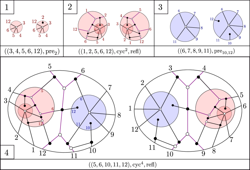
Figure 17. Illustration of building up a BCFW cell using the recipe $\mathfrak{r}$ of Example 6.17. Box $i$ shows the result after the first $i$ step-tuples. The result of the step $(a_{i},b_{i},c_{i},d_{i},n_{i})$ is shown on the left in each box, and the results of the steps $\mbox{pre}_{I_{i}},\mbox{cyc}^{r_{i}}$ and $\mbox{refl}^{s_{i}}$ are shown on the right.

Because our arguments are frequently recursive, we need some notation for the BCFW cells obtained by deleting the final step of a recipe. We use the following notation throughout.

Notation 6.18.

Let $\mathfrak{r}$ be a recipe for a BCFW cell $S\in\operatorname{Gr}_{k,N}^{\scriptscriptstyle\geq 0}$. Let FStep denote the final step, which is either $(a_{k},b_{k},c_{k},d_{k},n_{k}),\operatorname{pre}_{I_{k}},\operatorname{cyc}$ or $\operatorname{refl}$. If $\text{FStep}\neq(a_{k},b_{k},c_{k},d_{k},n_{k})$, then we let $\mathfrak{p}$ denote the recipe obtained by replacing FStep with the identity. Note that $S_{\mathfrak{p}}$ is again a BCFW cell. If $\text{FStep}=(a_{k},b_{k},c_{k},d_{k},n_{k})$, let $\mathfrak{r}_{L}$ and $\mathfrak{r}_{R}$ denote the recipes on $N_{L}$ and $N_{R}$ as in Definition 6.16. Then $\mathfrak{r}_{L},\mathfrak{r}_{R}$ are recipes for BCFW cells $S_{L}\subset\operatorname{Gr}_{k_{L},N_{L}}^{\scriptscriptstyle\geq 0}$ and $S_{R}\subset\operatorname{Gr}_{k_{R},N_{R}}^{\scriptscriptstyle\geq 0}$ and $S=S_{L}\bowtie S_{R}$. Note that to avoid clutter, we will usually use $L,R$ as subscripts rather than writing $S_{\mathfrak{r}_{L}},S_{\mathfrak{r}_{R}}$.

Remark 6.19.

In contrast with the bijective correspondence between standard BCFW cells and chord diagrams, multiple recipes could give rise to the same general BCFW cell. Even the sets of 5 indices that are involved in the BCFW products are not uniquely determined by the resulting cell.

We now construct a representative matrix for elements of a BCFW cell. We will use this matrix in the next section to invert the $\tilde{Z}$-map on BCFW cells (see Definition 7.1 and Theorem 7.7).

Definition 6.20 (BCFW parameters and matrix).

Let $\mathfrak{r}$ be a recipe on $N$ for a BCFW cell $S_{\mathfrak{r}}$. We define the BCFW parameters $\mathcal{C}_{\mathfrak{r}}$ and BCFW matrix $M_{\mathfrak{r}}$ of $S_{\mathfrak{r}}$ recursively. If $\mathfrak{r}$ is the trivial recipe, then $\mathcal{C}_{\mathfrak{r}}=\varnothing$ and $M_{\mathfrak{r}}$ is a $0\times N$ matrix. If $\text{FStep}=(a_{k},b_{k},c_{k},d_{k},n_{k})$, then let $\mathcal{C}_{L},\mathcal{C}_{R}$ and $M_{L},M_{R}$ be the BCFW parameters and matrices of $S_{L},S_{R}$. The BCFW parameters and matrix of $S_{\mathfrak{r}}$ are

$$\mathcal{C}_{\mathfrak{r}}\;:=\;\mathcal{C}_{L}\cup\{{\alpha}_{k},{\beta}_{k},{\delta}_{k},{\gamma}_{k},{\varepsilon}_{k}\}\cup\mathcal{C}_{R}\;=\;\{{\alpha}_{i},{\beta}_{i},{\delta}_{i},{\gamma}_{i},{\varepsilon}_{i}\}_{i=1}^{k}$$

$$M_{\mathfrak{r}}\;:=\;\iota_{\bowtie}(M_{L},[{\alpha}_{k}:{\beta}_{k}:{\delta}_{k}:{\gamma}_{k}:{\varepsilon}_{k}],M_{R}).$$

where in a slight abuse of notation, here $\iota_{\bowtie}(\dots)$ denotes the matrix $(*)$ from Figure 10 rather than its rowspan. If $\text{FStep}\in\{\operatorname{pre}_{I_{k}},\operatorname{cyc},\operatorname{refl}\}$, then we define $\mathcal{C}_{\mathfrak{r}}:=\mathcal{C}_{\mathfrak{p}}$ and $M_{\mathfrak{r}}:=\text{FStep}(M_{\mathfrak{p}})$.

We can think of the BCFW parameters ${\alpha}_{i},{\beta}_{i},{\gamma}_{i},{\delta}_{i},{\varepsilon}_{i}$ (for $1\leq i\leq k$) as abstract variables, but in Proposition 6.22, we will show that when they range over the positive real numbers, the corresponding BCFW matrices sweep out the BCFW cell $S_{\mathfrak{r}}$.

In words, $M_{\mathfrak{r}}$ is precisely the matrix obtained by following the sequence of operations given by $\mathfrak{r}$, and the BCFW parameters are exactly the $5k$ parameters used in the applications of $\iota_{\bowtie}$ as in Definition 5.2. The entries of $M_{\mathfrak{r}}$ are rational functions of the BCFW parameters $\mathcal{C}_{\mathfrak{r}}$ and may depend on the recipe $\mathfrak{r}$ chosen. Each row of the BCFW matrix is naturally indexed by a step-tuple in $\mathfrak{r}$. We will frequently use $\zeta_{i}\in\{{\alpha}_{i},{\beta}_{i},{\gamma}_{i},{\delta}_{i},{\varepsilon}_{i}\}$ (for $1\leq i\leq k$) to denote one BCFW parameter.

Example 6.21 (BCFW parameters and matrix).

We build the BCFW matrix $M_{\mathfrak{r}}$ of the cell $S_{\mathfrak{r}}$ from Example 6.17 in terms of the BCFW parameters $\{{\zeta}_{i}\}$. We will denote $(10,11,12)$ as $(A,B,C)$.

• (Step $1$): after last step of the first step-tuple:

  $$M_{L}^{(1)}=\blockarray{cccccc}2&3456C\\ \block{(cccccc)}0{\alpha}_{1}{\beta}_{1}{\gamma}_{1}{\delta}_{1}{\varepsilon}_{1}\\$$

• (Step $2$): after the first step of the second step-tuple $M_{L}^{(2)}=\iota_{\bowtie}(0,[{\alpha}_{2}:{\beta}_{2}:{\gamma}_{2}:{\delta}_{2}:{\varepsilon}_{2}],M_{L}^{(1)})$:

  $$M_{L}^{(2)}=\blockarray{ccccccc}1&23456C\\ \block{(ccccccc)}{\alpha}_{2}{\beta}_{2}00-{\gamma}_{2}-{\delta}_{2}-{\varepsilon}_{2}\\ 00{\alpha}_{1}{\beta}_{1}{\gamma}^{\prime}_{1}{\delta}^{\prime}_{1}{\varepsilon}_{1}\\ ,$$

  where: ${\delta}^{\prime}_{1}={\delta}_{1}+\frac{{\delta}_{2}}{{\varepsilon}_{2}}{\varepsilon}_{1}$ and ${\gamma}^{\prime}_{1}={\gamma}_{1}+\frac{{\gamma}_{2}}{{\delta}_{2}}{\delta}^{\prime}_{1}$. In Step $3$ we apply $\mbox{cyc}^{2}$ and refl to $M_{L}^{(2)}$ and get $M_{L}^{(3)}$.

• (Step $4$): after the last step of the third step-tuple:

  $$M_{R}=\blockarray{ccccccc}6&789ABC\\ \block{(ccccccc)}{\alpha}_{3}{\beta}_{3}{\gamma}_{3}{\delta}_{3}0{\varepsilon}_{3}0\\$$

• (Step $5$): after the first step of the fourth step-tuple $M^{(5)}=\iota_{\bowtie}(M_{L}^{(3)},[{\alpha}_{4}:{\beta}_{4}:{\gamma}_{4}:{\delta}_{4}:{\varepsilon}_{4}],M_{R}):$

  $$M^{(5)}=\blockarray{cccccccccccc}1&23456789ABC\\ \block{(cccccccccccc)}-{\gamma}_{2}00{\beta}_{2}{\alpha}^{\prime}_{2}{\varepsilon}_{2}00000{\delta}_{2}\\ {\gamma}^{\prime}_{1}{\beta}_{1}{\alpha}_{1}0-\mu_{1}-{\varepsilon}_{1}00000-{\delta}^{\prime}_{1}\\ 0000{\alpha}_{4}{\beta}_{4}000-{\gamma}_{4}-{\delta}_{4}-{\varepsilon}_{4}\\ 00000{\alpha}_{3}{\beta}_{3}{\gamma}_{3}{\delta}_{3}\nu_{3}{\varepsilon}_{3}0\\ ,$$

  where: ${\alpha}^{\prime}_{2}={\alpha}_{2}+\frac{{\alpha}_{4}}{{\beta}_{4}}{\varepsilon}_{2}$, $\mu_{1}=\frac{{\alpha}_{4}}{{\beta}_{4}}{\varepsilon}_{1}$, and $\nu_{3}=\frac{{\gamma}_{4}}{{\delta}_{4}}{\varepsilon}_{3}$. Finally, in order to get $M_{\mathfrak{r}}$, we apply $\mbox{cyc}^{4}$ and refl to $M^{(5)}$.

We now show that allowing the BCFW parameters to vary in $M_{\mathfrak{r}}$ gives a parametrization of $S_{\mathfrak{r}}$.

Proposition 6.22.

Let $\mathfrak{r}$ be a recipe for a BCFW cell $S_{\mathfrak{r}}$ with BCFW matrix $M_{\mathfrak{r}}$. Then the map

$$\left(\operatorname{Gr}_{1,5}^{\scriptscriptstyle>0}\right)^{k}\;\to\;S_{\mathfrak{r}}$$

$$\left([{\alpha}_{i}:{\beta}_{i}:{\gamma}_{i}:{\delta}_{i}:{\varepsilon}_{i}]\right)_{i=1}^{k}\;\mapsto\;M_{\mathfrak{r}}$$

sending the collection of BCFW parameters to the BCFW matrix $M_{\mathfrak{r}}$ is a bijection, where as usual we identify $M_{\mathfrak{r}}$ with its row span. In particular, $S_{\mathfrak{r}}$ has dimension 4k.

Given a recipe $\mathfrak{r}$, the BCFW parameters $\mathcal{C}_{\mathfrak{r}}$ of a point $V\in S_{\mathfrak{r}}$ are given (up to rescaling) by the preimage of $V$ under the bijection above.

Proof.

We proceed by induction on the number of steps in $\mathfrak{r}$. The base case is when $\mathfrak{r}$ is trivial, and is trivially true. If $\text{FStep}=\operatorname{pre}_{I_{k}},\operatorname{cyc}$ or $\operatorname{refl}$, the proposition for $S_{\mathfrak{r}}$ easily follows from the proposition for $S_{\mathfrak{p}}$. If $\text{FStep}=(a_{k},b_{k},c_{k},d_{k},n_{k})$, then this follows from the inductive hypothesis on $S_{L},S_{R}$ and Proposition 5.8, which we may apply because Corollary 10.7 shows that BCFW cells always satisfy the coindependence assumptions of 5.7. ∎

7. BCFW tiles and cluster adjacency

In this section we prove that the (closures of the) images of BCFW cells are tiles, and then state and prove the cluster adjacency theorem for general BCFW tiles. We note that our proof relies on a few technical ingredients that we defer to later sections.

7.1. BCFW tiles

Recall the definition of the amplituhedron map $\tilde{Z}$ from Definition 2.10, where $Z\in\operatorname{Mat}_{n,k+m}^{\scriptscriptstyle>0}$, and the definition of a tile from Definition 2.12. Our goal for this section is to use the BCFW matrix and parameters to invert the amplituhedron map on the image $Z_{\mathfrak{r}}^{\circ}=\tilde{Z}(S_{\mathfrak{r}})$ of each BCFW cell. Since Proposition 6.22 shows that BCFW cells in $\operatorname{Gr}_{k,n}^{\scriptscriptstyle\geq 0}$ have dimension $4k$, this will show that $Z_{\mathfrak{r}}$ is a tile.

The first step is to define one rational functionary for each BCFW parameter ${\zeta}_{i}\in\mathcal{C}_{\mathfrak{r}}$ where ${\zeta}\in\{{\alpha},{\beta},{\gamma},{\delta},{\varepsilon}\}$. The product promotion map $\Psi_{ac}$ (Definition 4.2) plays an integral role. The signs in the following definition are introduced such that each coordinate functionary is positive on the corresponding open tile (see Theorem 7.7).

Recall from Definition 2.9 the degree $\deg_{i}F$ of a functionary $F$ in an index $i$, and the operations $\operatorname{refl}^{*},\operatorname{cyc}^{-*}$ on functionaries (cf. Definition 2.3, Remark 3.21).

Definition 7.1 (Coordinate functionaries of BCFW cells).

Let $S_{\mathfrak{r}}\subset\operatorname{Gr}_{k,n}^{\scriptscriptstyle\geq 0}$ be a BCFW cell. For each BCFW parameter ${\zeta}_{i}\in\mathcal{C}_{\mathfrak{r}}$ we define the coordinate functionary ${\zeta}^{\mathfrak{r}}_{i}(Y)$ to be the function on $\operatorname{Gr}_{k,k+4}$ given by the following recursive definition:

• If $\text{FStep}=(a_{k},b_{k},c_{k},d_{k},n_{k})$, then we define

  $${\alpha}_{k}^{\mathfrak{r}}(Y)\,:=\,(-1)^{k_{R}}\langle\!\langle b_{k}\,c_{k}\,d_{k}\,n_{k}\rangle\!\rangle\quad\quad{\beta}_{k}^{\mathfrak{r}}(Y)\,:=\,(-1)^{k_{R}+1}\langle\!\langle a_{k}\,c_{k}\,d_{k}\,n_{k}\rangle\!\rangle$$

  $${\gamma}_{k}^{\mathfrak{r}}(Y)\,:=\,\langle\!\langle a_{k}\,b_{k}\,d_{k}\,n_{k}\rangle\!\rangle\quad\quad{\delta}_{k}^{\mathfrak{r}}(Y)\,:=\,-\langle\!\langle a_{k}\,b_{k}\,c_{k}\,n_{k}\rangle\!\rangle\quad\quad{\varepsilon}_{k}^{\mathfrak{r}}(Y)\,:=\,\langle\!\langle a_{k}\,b_{k}\,c_{k}\,d_{k}\rangle\!\rangle,$$

  and for $i\neq k$
  ${\zeta}^{\mathfrak{r}}_{i}(Y)\;:=\;\begin{cases}(-1)^{s}\Psi_{a_{k}c_{k}}({\zeta}_{i}^{L})(Y)\\ \Psi_{a_{k}c_{k}}({\zeta}_{i}^{R})(Y)\end{cases}$ if the $i$th step-tuple is in $\begin{cases}\mathfrak{r}_{L}\\ \mathfrak{r}_{R}\\ \end{cases},$ where $s=(k_{R}+1)\deg_{n_{k}}{\zeta}^{L}_{i}(Y)$.

• If $\text{FStep}=$ $\begin{cases}\operatorname{refl}\\ \operatorname{cyc}\\ \operatorname{pre}_{I_{k}}\end{cases}$ then ${\zeta}^{\mathfrak{r}}_{i}(Y):=\begin{cases}\operatorname{refl}^{*}{\zeta}^{\mathfrak{p}}_{i}(Y)\\ (-1)^{s^{\prime}}\operatorname{cyc}^{-*}{\zeta}^{\mathfrak{p}}_{i}(Y)\\ {\zeta}^{\mathfrak{p}}_{i}(Y)\end{cases}$, where $s^{\prime}=k\deg_{n}{\zeta}^{\mathfrak{p}}_{i}(Y)$.

We define the twistor matrix $M^{\operatorname{tw}}_{\mathfrak{r}}(Y)$ be the matrix $M_{\mathfrak{r}}$ of Definition 6.20 where each BCFW parameter ${\zeta}_{i}$ is set to equal the coordinate functionary ${\zeta}_{i}^{\mathfrak{r}}(Y)$. Its entries are rational functionaries.

Example 7.2 (Coordinate functionaries).

We will build recursively the coordinate functionaries $\{{\zeta}_{i}^{\mathfrak{r}}(Y)\}$ of the cell $S_{\mathfrak{r}}$ from Example 6.17. We will follow the same steps as in Example 6.21. We will denote $(10,11,12)$ as $(A,B,C)$ and $\{{\alpha}_{i}(Y),{\beta}_{i}(Y),{\gamma}_{i}(Y),{\delta}_{i}(Y),{\varepsilon}_{i}(Y)\}$ as $\{{\zeta}_{i}(Y)\}$ for brevity.

• (Step $1$): The coordinate functionaries $\{\zeta^{(1)}_{1}(Y)\}$ are respectively:

  $$\langle\!\langle 4\,5\,6\,C\rangle\!\rangle,-\langle\!\langle 3\,5\,6\,C\rangle\!\rangle,\langle\!\langle 3\,4\,6\,C\rangle\!\rangle,-\langle\!\langle 3\,4\,5\,C\rangle\!\rangle,\langle\!\langle 3\,4\,5\,6\rangle\!\rangle.$$

• (Step $2$): The coordinate functionaries $\{{\zeta}^{(2)}_{2}(Y)\}$ are respectively:

  $$-\langle\!\langle 2\,5\,6\,C\rangle\!\rangle,\langle\!\langle 1\,5\,6\,C\rangle\!\rangle,-\langle\!\langle 1\,2\,6\,C\rangle\!\rangle,\langle\!\langle 1\,2\,5\,C\rangle\!\rangle,-\langle\!\langle 1\,2\,5\,6\rangle\!\rangle.$$

  $\{{\zeta}^{(2)}_{1}(Y)\}$ are obtained as ${\zeta}^{(2)}_{1}=\Psi_{1,5}({\zeta}^{(1)}_{1})$ and are respectively:

  $$\langle\!\langle 4\,5\,6\,C\rangle\!\rangle,-\langle\!\langle 3\,5\,6\,C\rangle\!\rangle,\frac{\langle\!\langle 3\,4\,C\,|\,5\,6\,|\,1\,2\,C\rangle\!\rangle}{\langle\!\langle 1\,2\,5\,C\rangle\!\rangle},-\frac{\langle\!\langle 3\,4\,5\,|\,2\,1\,|\,5\,6\,C\rangle\!\rangle}{\langle\!\langle 1\,2\,5\,6\rangle\!\rangle},\langle\!\langle 3\,4\,5\,6\rangle\!\rangle.$$

• (Step $3$): $\{{\zeta}^{(3)}_{1}(Y)\}$ and $\{{\zeta}^{(3)}_{2}(Y)\}$ are obtained by performing $\operatorname{cyc}^{2}$ and $\operatorname{refl}$ on the respective coordinate functionaries of Step $2$.

• (Step $4$): The coordinate functionaries $\{{\zeta}^{(4)}_{3}(Y)\}$ are respectively:

  $$\langle\!\langle 7\,8\,9\,B\rangle\!\rangle,-\langle\!\langle 6\,8\,9\,B\rangle\!\rangle,\langle\!\langle 6\,7\,9\,B\rangle\!\rangle,-\langle\!\langle 6\,7\,8\,B\rangle\!\rangle,\langle\!\langle 6\,7\,8\,9\rangle\!\rangle.$$

• (Step $5$): The coordinate functionaries $\{{\zeta}^{(5)}_{4}(Y)\}$ are respectively:

  $$-\langle\!\langle 6\,A\,B\,C\rangle\!\rangle,\langle\!\langle 5\,A\,B\,C\rangle\!\rangle,-\langle\!\langle 5\,6\,B\,C\rangle\!\rangle,\langle\!\langle 5\,6\,A\,C\rangle\!\rangle,-\langle\!\langle 5\,6\,A\,B\rangle\!\rangle.$$

  $\{{\zeta}^{(5)}_{3}(Y)\}$ are obtained as ${\zeta}^{(5)}_{3}=\Psi_{5,10}({\zeta}^{(4)}_{3})$ and are respectively:

  $$\frac{\langle\!\langle 7\,8\,9\,|\,B\,A\,|\,5\,6\,C\rangle\!\rangle}{\langle\!\langle 5\,6\,A\,C\rangle\!\rangle},-\frac{\langle\!\langle 6\,8\,9\,|\,B\,A\,|\,5\,6\,C\rangle\!\rangle}{\langle\!\langle 5\,6\,A\,C\rangle\!\rangle},\frac{\langle\!\langle 6\,7\,9\,|\,B\,A\,|\,5\,6\,C\rangle\!\rangle}{\langle\!\langle 5\,6\,A\,C\rangle\!\rangle},-\frac{\langle\!\langle 6\,7\,8\,|\,B\,A\,|\,5\,6\,C\rangle\!\rangle}{\langle\!\langle 5\,6\,A\,C\rangle\!\rangle},\langle\!\langle 6\,7\,8\,9\rangle\!\rangle.$$

  $\{{\zeta}^{(5)}_{2}(Y)\}$ are obtained as ${\zeta}^{(5)}_{2}=\Psi_{5,10}({\zeta}^{(3)}_{2})$ and are respectively:

  $$-\frac{\langle\!\langle 1\,4\,C\,|\,5\,6\,|\,A\,B\,C\rangle\!\rangle}{\langle\!\langle 5\,A\,B\,C\rangle\!\rangle},\langle\!\langle 1\,5\,6\,C\rangle\!\rangle,-\langle\!\langle 4\,5\,6\,C\rangle\!\rangle,-\langle\!\langle 1\,4\,5\,6\rangle\!\rangle,\langle\!\langle 1\,4\,5\,C\rangle\!\rangle.$$

  $\{{\zeta}^{(5)}_{1}(Y)\}$ are obtained as ${\zeta}^{(5)}_{1}=\Psi_{5,10}({\zeta}^{(3)}_{1})$ and are respectively:

  $$\frac{\langle\!\langle 1\,2\,C\,|\,5\,6\,|\,A\,B\,C\rangle\!\rangle}{\langle\!\langle 5\,6\,B\,C\rangle\!\rangle},-\frac{\langle\!\langle 1\,3\,C\,|\,5\,6\,|\,A\,B\,C\rangle\!\rangle}{\langle\!\langle 5\,A\,B\,C\rangle\!\rangle},$$

  $$-\frac{\langle\!\langle A\,B\,C\,|\,5\,6\,|\,2\,3\,|\,1\,C\,|\,4\,5\,6\rangle\!\rangle}{\langle\!\langle 1\,4\,5\,6\rangle\!\rangle\langle\!\langle 5\,A\,B\,C\rangle\!\rangle},\frac{\langle\!\langle 1\,2\,3\,|\,4\,5\,|\,1\,2\,|\,5\,6\,|\,A\,B\,C\rangle\!\rangle}{\langle\!\langle 1\,4\,5\,C\rangle\!\rangle\langle\!\langle 5\,A\,B\,C\rangle\!\rangle},-\langle\!\langle 1\,2\,3\,C\rangle\!\rangle.$$

  Finally, $\{{\zeta}^{\mathfrak{r}}_{i}(Y)\}$ are obtained by applying $\operatorname{cyc}^{4},\operatorname{refl}$ on the coordinate functionaries of Step $5$.

The twistor matrix $M^{\operatorname{tw}}_{\mathfrak{r}}(Y)$ is obtained from the BCFW matrix $M_{\mathfrak{r}}$ in Example 6.21 by setting each BCFW parameter ${\zeta}^{\mathfrak{r}}_{i}$ equal to the corresponding coordinate functionary ${\zeta}^{\mathfrak{r}}_{i}(Y)$ computed above.

It is also convenient to define the following variant of the coordinate functionaries, which will be cluster variables for $\operatorname{Gr}_{4,n}$. The definition is based on rescaled product promotion $\overline{\Psi}$ (Definition 4.8).

Definition 7.3 (Coordinate cluster variables of BCFW cells).

Let $S_{\mathfrak{r}}\subset\operatorname{Gr}_{k,n}^{\scriptscriptstyle\geq 0}$ be a BCFW cell. For each BCFW parameter ${\zeta}_{i}\in\mathcal{C}_{\mathfrak{r}}$ the coordinate cluster variables $\bar{\zeta}^{\mathfrak{r}}_{i}$ is defined as follows:

• If $\text{FStep}=(a_{k},b_{k},c_{k},d_{k},n_{k})$, then we define

  $$\bar{\alpha}_{k}^{\mathfrak{r}}\,:=\,\langle b_{k}\,c_{k}\,d_{k}\,n_{k}\rangle\quad\quad\bar{\beta}_{k}^{\mathfrak{r}}\,:=\,\langle a_{k}\,c_{k}\,d_{k}\,n_{k}\rangle$$

  $$\bar{\gamma}_{k}^{\mathfrak{r}}\,:=\,\langle a_{k}\,b_{k}\,d_{k}\,n_{k}\rangle\quad\quad\bar{\delta}_{k}^{\mathfrak{r}}\,:=\,\langle a_{k}\,b_{k}\,c_{k}\,n_{k}\rangle\quad\quad\bar{\varepsilon}_{k}^{\mathfrak{r}}\,:=\,\langle a_{k}\,b_{k}\,c_{k}\,d_{k}\rangle,\vspace{1em}$$

  and for $i\neq k$,  $\bar{\zeta}^{\mathfrak{r}}_{i}\;:=\;\begin{cases}\overline{\Psi}_{a_{k}c_{k}}(\bar{\zeta}_{i}^{L})\\ \overline{\Psi}_{a_{k}c_{k}}(\bar{\zeta}_{i}^{R})\end{cases}$ if the $i$th step-tuple is in $\begin{cases}\mathfrak{r}_{L}\\ \mathfrak{r}_{R}\\ \end{cases}.$

• If $\text{FStep}=$ $\begin{cases}\operatorname{refl}\\ \operatorname{cyc}\\ \operatorname{pre}_{I_{k}}\end{cases}$ then $\bar{\zeta}^{\mathfrak{r}}_{i}:=\begin{cases}\operatorname{refl}^{*}\bar{\zeta}^{\mathfrak{p}}_{i}\\ \operatorname{cyc}^{-*}\bar{\zeta}^{\mathfrak{p}}_{i}\\ \bar{\zeta}^{\mathfrak{p}}_{i}\end{cases}$.

We denote the set of coordinate cluster variables for $S_{\mathfrak{r}}$ by $\operatorname{\mathbf{x}}(\mathfrak{r})$. Note that $\operatorname{\mathbf{x}}(\mathfrak{r})$ depends on the recipe $\mathfrak{r}$ rather than just the BCFW cell.

Example 7.4 (Coordinate cluster variables).

We will build recursively the coordinate cluster variables $\{\bar{\zeta}_{i}^{\mathfrak{r}}\}$ of the cell $S_{\mathfrak{r}}$ from Example 6.17. We will follow the same steps as in Example 6.21 and Example 7.2. We will denote $(10,11,12)$ as $(A,B,C)$ and $\{\bar{\alpha}_{i},\bar{\beta}_{i},\bar{\gamma}_{i},\bar{\delta}_{i},\bar{\varepsilon}_{i}\}$ as $\{\bar{\zeta}_{i}\}$ for brevity.

• (Step $1$): The coordinate cluster variables $\{\bar{\zeta}^{(1)}_{1}\}$ are respectively:

  $$\langle 4\,5\,6\,C\rangle,\langle 3\,5\,6\,C\rangle,\langle 3\,4\,6\,C\rangle,\langle 3\,4\,5\,C\rangle,\langle 3\,4\,5\,6\rangle.$$

• (Step $2$): The coordinate cluster variables $\{\bar{\zeta}^{(2)}_{2}\}$ are respectively:

  $$\langle 2\,5\,6\,C\rangle,\langle 1\,5\,6\,C\rangle,\langle 1\,2\,6\,C\rangle,\langle 1\,2\,5\,C\rangle,\langle 1\,2\,5\,6\rangle.$$

  $\{\bar{\zeta}^{(2)}_{1}\}$ are obtained as $\bar{\zeta}^{(2)}_{1}=\overline{\Psi}_{1,5}(\bar{\zeta}^{(1)}_{1})$ and are respectively:

  $$\langle 4\,5\,6\,C\rangle,\langle 3\,5\,6\,C\rangle,\langle 3\,4\,C\,|\,5\,6\,|\,1\,2\,C\rangle,\langle 3\,4\,5\,|\,2\,1\,|\,5\,6\,C\rangle,\langle 3\,4\,5\,6\rangle.$$

• (Step $3$): $\{\bar{\zeta}^{(3)}_{1}\}$ and $\{\bar{\zeta}^{(3)}_{2}\}$ are obtained by performing $\operatorname{cyc}^{2}$ and $\operatorname{refl}$ on the respective coordinate cluster variables of Step $2$.

• (Step $4$): The coordinate cluster variables $\{\bar{\zeta}^{(4)}_{3}\}$ are respectively:

  $$\langle 7\,8\,9\,B\rangle,\langle 6\,8\,9\,B\rangle,\langle 6\,7\,9\,B\rangle,\langle 6\,7\,8\,B\rangle,\langle 6\,7\,8\,9\rangle.$$

• (Step $5$): The coordinate cluster variables $\{\bar{\zeta}^{(5)}_{4}\}$ are respectively:

  $$\langle 6\,A\,B\,C\rangle,\langle 5\,A\,B\,C\rangle,\langle 5\,6\,B\,C\rangle,\langle 5\,6\,A\,C\rangle,\langle 5\,6\,A\,B\rangle.$$

  $\{\bar{\zeta}^{(5)}_{3}\}$ are obtained as $\bar{\zeta}^{(5)}_{3}=\overline{\Psi}_{5,10}(\bar{\zeta}^{(4)}_{3})$ and are respectively:

  $$\langle 7\,8\,9\,|\,B\,A\,|\,5\,6\,C\rangle,\langle 6\,8\,9\,|\,B\,A\,|\,5\,6\,C\rangle,\langle 6\,7\,9\,|\,B\,A\,|\,5\,6\,C\rangle,\langle 6\,7\,8\,|\,B\,A\,|\,5\,6\,C\rangle,\langle 6\,7\,8\,9\rangle.$$

  $\{\bar{\zeta}^{(5)}_{2}\}$ are obtained as $\bar{\zeta}^{(5)}_{2}=\overline{\Psi}_{5,10}(\bar{\zeta}^{(3)}_{2})$ and are respectively:

  $$\langle 1\,4\,C\,|\,5\,6\,|\,A\,B\,C\rangle,\langle 1\,5\,6\,C\rangle,\langle 4\,5\,6\,C\rangle,\langle 1\,4\,5\,6\rangle,\langle 1\,4\,5\,C\rangle.$$

  $\{\bar{\zeta}^{(5)}_{1}\}$ are obtained as $\bar{\zeta}^{(5)}_{1}=\overline{\Psi}_{5,10}(\bar{\zeta}^{(3)}_{1})$ and are respectively:

  $$\langle 1\,2\,C\,|\,5\,6\,|\,A\,B\,C\rangle,\langle 1\,3\,C\,|\,5\,6\,|\,A\,B\,C\rangle,$$

  $$\langle A\,B\,C\,|\,5\,6\,|\,2\,3\,|\,1\,C\,|\,4\,5\,6\rangle,\langle 1\,2\,3\,|\,4\,5\,|\,1\,C\,|\,5\,6\,|\,A\,B\,C\rangle,\langle 1\,2\,3\,C\rangle.$$

  Finally, $\{\bar{\zeta}^{\mathfrak{r}}_{i}\}$ are obtained by applying $\operatorname{cyc}^{4},\operatorname{refl}$ on the coordinate cluster variables of Step $5$.

Remark 7.5 (Chain polynomials and beyond).

In Theorem 8.4, we will show that coordinate cluster variables for standard BCFW cells are always chain polynomials (cf. Definition 2.5). However, this is not the case for general BCFW cells. To describe a specific example $S_{\mathfrak{r}}$ on $N=\{1,\dots,\mathrm{C}\}$, we start with the standard BCFW cell corresponding to the chord diagram

$$D^{\prime}\;=\;((3,7,8,9),(8,9,\mathrm{A},\mathrm{B}),(1,2,\mathrm{A},\mathrm{B}))\quad\text{with}\quad N^{\prime}=\{1,2,3,7,8,9,\mathrm{A},\mathrm{B},\mathrm{C}\}.$$

Using Theorem 8.4, we have $\bar{\gamma}_{1}^{D^{\prime}}\;=\;\langle\mathrm{C}\,\mathrm{A}\,\mathrm{B}\,|\,2\,1\,|\,3\,7\,|\,8\,9\,|\,\mathrm{A}\,\mathrm{B}\,\mathrm{C}\rangle\,.$ This variable is preserved after an application of $\operatorname{pre}_{\{4,6\}}$. Then, after suitable reflections and rotations, we can apply upper promotion, which in terms of the original indices of $D^{\prime}$ takes place at $(a,b,c,d,n)\;=\;(5,4,8,7,6).$ The above cluster variable promotes using the rule $7\mapsto 7-\tfrac{\langle 5\,4\,7\,6\rangle}{\langle 5\,4\,8\,6\rangle}8$, and yields

$$\bar{\gamma}_{1}^{\mathfrak{r}}\;=\;\overline{\Psi}(\bar{\gamma}_{1}^{D^{\prime}})\;=\;\langle\mathrm{C}\,\mathrm{A}\,\mathrm{B}\,|\,2\,1\,|\,3\,7\,|\,8\,9\,|\,\mathrm{A}\,\mathrm{B}\,\mathrm{C}\rangle\langle 4\,5\,6\,8\rangle+\langle\mathrm{C}\,\mathrm{A}\,\mathrm{B}\,|\,2\,1\,|\,3\,7\,9\rangle\langle 8\,\mathrm{A}\,\mathrm{B}\,\mathrm{C}\rangle\langle 4\,5\,6\,7\rangle.$$

This expression further expands to an irreducible quartic polynomial in Plücker coordinates with $8$ terms, which cannot be written as a chain polynomial.

Lemma 7.6.

Let $\mathfrak{r}$ be a recipe for a BCFW cell. Then the coordinate cluster variables $\operatorname{\mathbf{x}}(\mathfrak{r})$ are a collection of compatible cluster variables for $\operatorname{Gr}_{4,n}$.

Proof.

We prove this by induction on the number of step-tuples in $\mathfrak{r}$. The base case is trivial. If the final step is $\operatorname{cyc},\operatorname{refl}$ or $\operatorname{pre}_{i}$, the statement follows from the inductive hypothesis and Corollaries 3.18 and 3.20, which assert that $\operatorname{cyc}^{-*},\operatorname{refl}^{*}$ and the inclusion map send cluster variables to cluster variables and preserve compatibility. If the final step is $(a,b,c,d,n)$, then the definition of $\overline{\Psi}$ implies that $\operatorname{\mathbf{x}}(\mathfrak{r})$ consists of cluster variables for $\operatorname{Gr}_{4,n}$. To see compatibility, note that by induction, $\operatorname{\mathbf{x}}(\mathfrak{r}_{L})\sqcup\operatorname{\mathbf{x}}(\mathfrak{r}_{R})$ is a set of compatible cluster variables for $\mathbb{C}[\widehat{\operatorname{Gr}}_{4,N_{L}}]\times\mathbb{C}[\widehat{\operatorname{Gr}}_{4,N_{R}}]$. By Theorem 4.7 and the definition of $\overline{\Psi}$, applying $\overline{\Psi}$ to $\operatorname{\mathbf{x}}(\mathfrak{r}_{L})\sqcup\operatorname{\mathbf{x}}(\mathfrak{r}_{R})$ gives a collection of compatible cluster variables for $\operatorname{Gr}_{4,n}$. Moreover, these cluster variables are compatible with the Plücker coordinates $\langle abcd\rangle,\langle abcn\rangle,\langle abdn\rangle,\langle acdn\rangle,\langle bcdn\rangle$, which are all frozen in $\operatorname{Fr}(\Sigma_{1})$. This completes the proof of the lemma. ∎

We now state one of our main theorems. It says that the amplituhedron map $\tilde{Z}$ is injective on each BCFW cell $S_{\mathfrak{r}}$, giving an inverse map in terms of the coordinate functionaries. This shows that $Z_{\mathfrak{r}}$ is a tile. Moreover, it describes each open tile $Z_{\mathfrak{r}}$ as a semi-algebraic set in $\operatorname{Gr}_{k,k+4}$. It will be proved in Section 11.5..

Theorem 7.7 (General BCFW cells give tiles).

Let $S_{\mathfrak{r}}$ be a general BCFW cell with recipe $\mathfrak{r}$. Then for all $Z\in\operatorname{Mat}_{n,k+4}^{>0}$, $\tilde{Z}$ is injective on $S_{\mathfrak{r}}$ and thus $Z_{\mathfrak{r}}$ is a tile. In particular, given $Y\in\tilde{Z}(S_{\mathfrak{r}})$, the unique preimage of $Y$ in $S_{\mathfrak{r}}$ is given by (the rowspan of) of the twistor matrix $M^{\operatorname{tw}}_{\mathfrak{r}}(Y)$. Moreover,

$$Z_{\mathfrak{r}}^{\circ}=\{Y\in\operatorname{Gr}_{k,k+4}:{\zeta}_{i}^{\mathfrak{r}}(Y)>0\text{ for all coordinate functionaries of }S_{\mathfrak{r}}\}.$$

Theorem 7.7 allows us to make the following definition.

Definition 7.8 (BCFW tiles).

A general (respectively, standard) BCFW tile $Z_{S}$ is the closure $\overline{\tilde{Z}(S)}$ of the image of a general (respectively, standard) BCFW cell $S$. If the BCFW cell has the form $S_{\mathfrak{r}}$ (respectively, $S_{D}$) for a recipe $\mathfrak{r}$ (respectively, chord diagram $D$), then we also denote the corresponding tile by $Z_{\mathfrak{r}}$ (respectively, $Z_{D}$).

Example 7.9.

Given the cell $S_{\mathfrak{r}}\subset\operatorname{Gr}_{4,12}$ obtained by the recipe of Example 6.17, then $Z_{\mathfrak{r}}$ is a tile for $\mathcal{A}_{12,4,4}(Z)$. Moreover, $Z_{\mathfrak{r}}^{\circ}$ is the region in $\operatorname{Gr}_{4,8}$ where all the coordinate functionaries $\{{\zeta}^{\mathfrak{r}}_{i}(Y)\}$ in Example 7.2 are positive.

Example 7.10.

For $k=1$, the amplituhedron $\mathcal{A}_{n,1,4}(Z)$ is a cyclic polytope in $\mathbb{P}^{4}$ whose vertices are the $n$ rows of $Z$. The $k=1$ BCFW tiles are exactly the full-dimensional simplices whose vertices are vertices of the cyclic polytope $\mathcal{A}_{n,1,4}(Z)$. In particular, the tile corresponding to the BCFW cell on the right in Figure 14 is the simplex with vertices $Z_{a},Z_{b},Z_{c},Z_{d},Z_{e}$.

	$0$	$1$	$2$	$3$	$4$	$5$	$6$	$7$	$8$	$9$
$5$	$1$	$1$
$6$	$1$	$6$	$1$
$7$	$1$	$21$	$21$	$1$
$8$	$1$	$56$	$176$	$56$	$1$
$9$	$1$	$126$	$939$	$939$	$126$	$1$
$10$	$1$	$252$	$3785$	$8690$	$3785$	$252$	$1$
$11$	$1$	$462$	$12562$	$55847$	$55847$	$12562$	$462$	$1$
$12$	$1$	$792$	$36102$	$279148$	$534258$	$279148$	$36102$	$792$	$1$
$13$	$1$	$1287$	$92807$	$1158664$	$3795064$	$3795064$	$1158664$	$92807$	$1287$	$1$

Table 1. Number of BCFW tiles of $\mathcal{A}_{n,k,4}(Z)$. For comparison, the standard BCFW tiles of $\mathcal{A}_{13,4,4}(Z)$ consists of 5292 out of the 3795064 general BCFW tiles.

Notation 7.11.

Given a cluster variable $x$ in $\operatorname{Gr}_{4,n}$, we will denote as $x(Y)$ the functionary on $\operatorname{Gr}_{k,k+4}$ obtained by identifying Plücker coordinates $\langle I\rangle$ on $\operatorname{Gr}_{4,n}$ with twistor coordinates $\langle\!\langle I\rangle\!\rangle$ on $\operatorname{Gr}_{k,k+4}$, see Section 2.5. When it is clear from the context, we will talk about cluster variables and the corresponding functionaries interchangeably.

Theorem 7.7 gives a description of each open BCFW tile as a semi-algebraic set in $\operatorname{Gr}_{k,k+4}$, cut out by the positivity of the coordinate functionaries. Each coordinate functionary is a (signed) Laurent monomial in the coordinate cluster variables, and vice versa. Using Theorem 7.7 and the ingredients in its proof, we can obtain a description of the open tile using cluster variables.

Corollary 7.12 (Sign description for general BCFW tiles).

Let $Z_{\mathfrak{r}}$ be a general BCFW tile. For each element $x$ of $\operatorname{\mathbf{x}}(\mathfrak{r})$, the functionary $x(Y)$ has a definite sign $s_{x}$ on $Z_{\mathfrak{r}}^{\circ}$ and

$$Z_{\mathfrak{r}}^{\circ}=\{Y\in\operatorname{Gr}_{k,k+4}:s_{x}\,x(Y)>0\text{ for all }x\in\operatorname{\mathbf{x}}(\mathfrak{r})\}.$$

Proof.

Corollary 11.18 shows that for each element $x$ of $\operatorname{\mathbf{x}}(\mathfrak{r})$, the functionary $x(Y)$ has a definite sign $s_{x}$ on $Z_{\mathfrak{r}}^{\circ}$. This implies that $Z_{\mathfrak{r}}^{\circ}\subset\{Y\in\operatorname{Gr}_{k,k+4}:s_{x}\,x(Y)>0\text{ for all }x\in\operatorname{\mathbf{x}}(\mathfrak{r})\},$ so all that remains is the reverse inclusion. By Theorem 7.7, $Z_{\mathfrak{r}}^{\circ}$ is the subset of $\operatorname{Gr}_{k,k+4}$ where the coordinate functionaries are positive, so it suffices to show that the coordinate functionaries are positive on the points in the right hand set.

Suppose $Y\in\operatorname{Gr}_{k,k+4}$ satisfies $s_{x}x(Y)>0$ for all coordinate cluster variables. Comparing the definition of the coordinate functionaries in Definition 7.1 to the definition of the coordinate cluster variables in Definition 7.3, we see that each coordinate functionary is a signed Laurent monomial in the coordinate cluster variables. Thus, the signs $s_{x}$ of the coordinate cluster variables imply that each coordinate functionary $\zeta$ also has a particular sign on $Y$. This sign must be positive, since $x(Y^{\prime})$ has sign $s_{x}$ on any $Y^{\prime}$ in the tile $Z_{\mathfrak{r}}^{\circ}$ and every coordinate functionary is positive on $Y^{\prime}$. ∎

One may compute the signs $s_{x}$ in Corollary 7.12 recursively using Theorems 11.2, 11.3 and 9.34.

Remark 7.13 (Relevance to physics).

A connection between certain positroid cells in $\operatorname{Gr}^{\geq 0}_{k,n}$ and cluster variables in $\operatorname{Gr}_{4,n}$ was explored in [MSSV20, HL21]. The authors consider a positive parametrisation of positroid cells using edge or face variables of an associated plabic graph. Then by solving the ‘$C\cdot z$ equations’, they express these variables as ratios of elements of $\mathbb{C}[\operatorname{Gr}_{4,n}]$. They observe that most of the polynomials appearing are cluster variables for $\operatorname{Gr}_{4,n}$ and are relevant for the symbol alphabet of loop amplitudes in $\mathcal{N}=4$ SYM. However, they also note that there are polynomials which are not cluster variables. We observe that for a positroid cell $S$ which gives a tile $Z_{S}$, solving the ‘$C\cdot z$ equations’ is equivalent to inverting the amplituhedron map $\tilde{Z}$ on $Z_{S}$. In this section (see Definition 7.3, Theorem 7.7 and Corollary 7.12) we showed that, parametrising a BCFW cell $S_{\mathfrak{r}}$ using BCFW parameters $\zeta_{i}\in\mathcal{C}_{\mathfrak{r}}$, one may express all $\zeta_{i}$ as ratios of cluster variables in $\operatorname{Gr}_{4,n}$ (thought as functionaries in $\mbox{Gr}_{k,k+4}$). Morover, changing the recipe $\mathfrak{r}$ for a BCFW cell may give a different set of cluster variables. It would be interested to explore the relevance of all such cluster variables for the symbol alphabet and loop amplitudes.

Example 7.14 (Sign description of BCFW tiles).

Consider the tile $Z_{\mathfrak{r}}$ in $\mathcal{A}_{12,4,4}(Z)$, where $\mathfrak{r}$ is the recipe from Example 6.17. Then, $Z_{\mathfrak{r}}^{\circ}$ is the region in $\operatorname{Gr}_{4,8}$ where all the coordinate cluster variables $\{\bar{\zeta}^{\mathfrak{r}}_{i}\}$ in Example 7.4 – thought as functionaries – have a certain definite sign. Note that their signs is determined by the positivity of the coordinate functionaries in Example 7.2 (and vice-versa).

7.2. Cluster adjacency for BCFW tiles

Now we turn to cluster adjacency for general BCFW tiles. Recall from Definition 2.14 the notion of a facet of $Z_{\mathfrak{r}}$. We will use the following theorem (a special case of Theorems 11.2 and 11.3) to find functionaries which vanish on facets of $Z_{\mathfrak{r}}$. Recall 2.11 and the definition of product promotion $\Psi$ from Definition 4.2.

Theorem 7.15.

1. Let $S\subset\operatorname{Gr}_{k,n}^{\scriptscriptstyle\geq 0}$ be a positroid cell. Suppose that $F$ is a pure rational functionary which vanishes on $Z_{S}$ for all $Z$. Then

   $$\begin{cases}F\\ \operatorname{cyc}^{-*}F\\ \operatorname{refl}^{*}F\end{cases}\text{ vanishes on }\begin{cases}Z_{\operatorname{pre}_{I}S}\\ Z_{\operatorname{cyc}S}\\ Z_{\operatorname{refl}S}\end{cases},\quad\mbox{for all }Z.$$

2. Let $S_{L}\subset\operatorname{Gr}_{k_{L},N_{L}}$ and $S_{R}\subset\operatorname{Gr}_{k_{R},N_{R}}$ be positroid cells as in 5.7. Let $F$ be a pure functionary with indices contained in $N_{L}$ (resp. $N_{R}$) which vanishes on $Z_{S_{L}}$ (resp. $Z_{S_{R}}$) for all $Z$. Then $\Psi(F)$ vanishes on $Z_{S_{L}\bowtie S_{R}}$ for all $Z$.

Using Theorem 7.15 and Lemma 10.5, we can prove the following theorem.

Theorem 7.16 (Cluster adjacency for general BCFW tiles).

Let $Z_{\mathfrak{r}}$ be a general BCFW tile of $\mathcal{A}_{n,k,4}({Z})$. Each facet $Z_{S}$ of $Z_{\mathfrak{r}}$ lies on a hypersurface cut out by a functionary $F_{S}(\langle\!\langle I\rangle\!\rangle)$ such that $F_{S}(\langle I\rangle)\in\operatorname{\mathbf{x}}(\mathfrak{r})$. Thus $\{F_{S}(\langle I\rangle):Z_{S}\text{ a facet of }Z_{\mathfrak{r}}\}$ consists of compatible cluster variables of $\operatorname{Gr}_{4,n}$.

Proof.

Note that by Lemma 7.6, $\operatorname{\mathbf{x}}(\mathfrak{r})$ consists of compatible cluster variables for $\operatorname{Gr}_{4,n}$ (under the usual identification of Plücker coordinates and twistor coordinates). So the final sentence of the theorem statement follows from the second sentence. To prove the second sentence, we will show the following claim.

Claim: Let $S\subset\overline{S_{\mathfrak{r}}}$ be a cell in the boundary of $S_{\mathfrak{r}}$. Then for all $Z$, $Z_{S}$ lies in the vanishing locus of an element of $\operatorname{\mathbf{x}}(\mathfrak{r})$.

We prove the claim by induction on the number of steps in $\mathfrak{r}$. We will use the notation of 6.18. For the base case ($k=0$ and $\mathfrak{r}=\emptyset$), there is nothing to prove. If $\text{FStep}=\operatorname{pre}_{I}$, then the map $\operatorname{pre}_{I}$ is a stratification-preserving homeomorphism from $\overline{S_{\mathfrak{p}}}$ to $\overline{S_{\mathfrak{r}}}$. That is, any cell in the boundary of $S_{\mathfrak{r}}$ is of the form $\operatorname{pre}_{I}(S)$ for some $S$ in the boundary of $S_{\mathfrak{p}}$. By the inductive hypothesis, there is some functionary $F\in\operatorname{\mathbf{x}}(\mathfrak{p})$ which vanishes on $Z_{S}$ for all $Z$. By Theorem 7.15, $F$ also vanishes on $Z_{\operatorname{pre}_{I}S}$ for all $Z$. By Definition 7.3, $F$ is also an element of $\operatorname{\mathbf{x}}(\mathfrak{r})$, so the claim holds in this case. The arguments for $\text{FStep}=\operatorname{cyc}$ or $\text{FStep}=\operatorname{refl}$ are analogous.

If $\text{FStep}=(a,b,c,d,n)$, then by Lemma 10.5 the boundary of $S_{\mathfrak{r}}$ consists of (1) cells of the form $S_{L}^{\prime}\bowtie S_{R}^{\prime}$ where $S_{L}^{\prime}\subseteq\overline{S_{L}},S_{R}^{\prime}\subseteq\overline{S_{R}}$, $(S_{L}^{\prime},S_{R}^{\prime})\neq(S_{L},S_{R})$ and $\{a,b,n\},\{b,c,d,n\}$ are coindependent for $S_{L}^{\prime},S_{R}^{\prime}$, respectively; and (2) cells for which some element of $\binom{\{a,b,c,d,n\}}{4}$ fails to be coindependent.

Consider a cell $S_{L}^{\prime}\bowtie S_{R}^{\prime}$ appearing in (1) and suppose $S_{L}^{\prime}\neq S_{L}$. By the inductive hypothesis on $S_{L}$, there is a functionary $F\in\operatorname{\mathbf{x}}(L)$ which vanishes on $Z_{S_{L}^{\prime}}$ for all $Z$. By Theorem 7.15, the promotion $\Psi(F)$ vanishes on $Z_{S_{L}^{\prime}\bowtie S_{R}^{\prime}}$ for all $Z$. By Lemma 11.4, the twistor coordinates $\langle\!\langle bcdn\rangle\!\rangle$, $\langle\!\langle acdn\rangle\!\rangle$, $\langle\!\langle abdn\rangle\!\rangle$, $\langle\!\langle abcn\rangle\!\rangle$, $\langle\!\langle abcd\rangle\!\rangle$ are nonvanishing on $Z_{S_{L}^{\prime}\bowtie S_{R}^{\prime}}$. So in fact the rescaled product promotion $\overline{\Psi}(F)$ vanishes on $Z_{S_{L}^{\prime}\bowtie S_{R}^{\prime}}$ for all $Z$. By Definition 7.3, $\overline{\Psi}(F)$ is also an element of $\operatorname{\mathbf{x}}(\mathfrak{r})$. This proves the claim for boundary cells of the form $S_{L}^{\prime}\bowtie S_{R}^{\prime}$ where $S_{L}^{\prime}\neq S_{L}$. An analogous argument shows the claim for the boundary cells of the form $S_{L}\bowtie S_{R}^{\prime}$.

Now, let $S$ be a cell in (2), and say $I$ is an element of $\binom{\{a,b,c,d,n\}}{4}$ which is not coindependent for $S$. This means that every basis of $S$ has nonempty intersection with $I$. Consider the twistor coordinate $\langle\!\langle I\rangle\!\rangle$. for all $Z$, every term in the sum (4) is equal to zero. So $\langle\!\langle I\rangle\!\rangle$ vanishes on $Z_{S}$ for all $Z$. By Definition 7.3, $\langle\!\langle I\rangle\!\rangle$ is in $\operatorname{\mathbf{x}}(\mathfrak{r})$ (it is one of the five twistor coordinates added). This concludes the proof of the claim.

Now, the claim implies the theorem. Indeed, any facet of $Z_{\mathfrak{r}}$ is by definition $Z_{S}$ for some cell $S\subset\overline{S_{\mathfrak{r}}}$. By the claim, $Z_{S}$ lies in the vanishing locus of an element of $\operatorname{\mathbf{x}}(\mathfrak{r})$ for any choice of $Z$. ∎

We believe that one can generalize Theorem 7.16 and Corollary 7.12 as follows.

Conjecture 7.17 (Cluster adjacency and positivity tests for tiles).

Let $Z_{S^{\prime}}$ be a tile of the amplituhedron $\mathcal{A}_{n,k,m}(Z)$.

1. (Cluster adjacency): Then for each facet $Z_{S}$ of $Z_{S^{\prime}}$, there is a functionary $F_{S}(\langle\!\langle I\rangle\!\rangle)$ which vanishes on $Z_{S}$, such that the collection

   $$\mathcal{F}=\{F_{S}(\langle I\rangle):Z_{S}\text{ a facet of }Z_{S^{\prime}}\}$$

   is a collection of compatible cluster variables for $\operatorname{Gr}_{m,n}$.

2. (Positivity test): Moreover for even $m$, given any extended cluster $\widetilde{\mathbf{x}}$ for $\operatorname{Gr}_{m,n}$ containing $\mathcal{F}$, there are signs $s_{x}\in\{1,-1\}$ for each $x\in\widetilde{\mathbf{x}}$, such that

   $$Z_{S}^{\circ}=\{Y\in\operatorname{Gr}_{k,k+m}:s_{x}\cdot x(Y)>0\text{ for all }x\in\widetilde{\mathbf{x}}\},$$

   where as in 7.11, $x(Y)$ is the functionary corresponding to the cluster variable $x$.

We will prove 7.17 for standard BCFW tiles in Section 9 (see Theorem 9.11), and for a non-BCFW tile (the ‘spurion’) in our companion paper [ELP⁺24] for the $m=4$ amplituhedron.

8. Cluster variables for standard BCFW tiles

In this section, we focus on standard BCFW tiles $Z_{D}$. We give explicit formulas for the coordinate cluster variables $\operatorname{\mathbf{x}}(D)$ (cf. Definition 7.3) in Theorem 8.4. We give explicit formulas for the sign of each element of $\operatorname{\mathbf{x}}(D)$ on the open tile $Z_{D}^{\circ}$ in Proposition 8.10.

8.1. Domino Cluster Variables

We first rewrite Definition 7.3 in the standard BCFW case using the combinatorics of chord diagrams. For a standard BCFW tile $Z_{D}$, we call the coordinate cluster variables domino cluster variables or simply domino variables. The terminology comes from [KWZ20] and [ELT21], where some related variables were used for entries of matrices parametrizing BCFW cells. The term “domino” was used for such variables, since the vectors and matrices tended to have adjacent pairs of nonzero same-sign entries, such as $\alpha,\beta$ and $\gamma,\delta$ in Figure 10.

Definition 8.1 (Domino cluster variables).

Let $D$ be a chord diagram in $\mathcal{CD}_{n,k}$, and let $D_{\operatorname{{\it k}}}=(a,b,c,d)$ denote the rightmost top chord, where $1\leq a<b<c<d<n$, and moreover $a,b$ and $c,d$ are consecutive. We define the domino (cluster) variables $\mathbf{x}(D)=\{\bar{\alpha}_{i},\bar{\beta}_{i},\bar{\gamma}_{i},\bar{\delta}_{i},\bar{\varepsilon}_{i}\ |\ 1\leq i\leq k\}$ recursively as follows, using the rescaled product promotion $\overline{\Psi}$ from Definition 4.8.

• (Removing the penultimate marker) If $d<n-1$, let $D^{\prime}$ be the chord diagram on $[n]\setminus\{n-1\}$ obtained from $D$ by removing the marker $n-1$. For any chord $D_{j}$ of $D$, and for $\bar{\zeta}\in\{\bar{\alpha},\bar{\beta},\bar{\gamma},\bar{\delta},\bar{\varepsilon}\}$:

  $$\bar{\zeta}_{j}^{D}\;=\;\bar{\zeta}_{j}^{D^{\prime}}$$

• (Removing the rightmost top chord) Otherwise, if $d=n-1$,

  the domino variables of $D$ are obtained from those of the left and right subdiagrams $D_{L},D_{R}$ (cf Definition 6.10) as follows.

  • The domino variables associated to the top chord $D_{\operatorname{{\it k}}}$ are given by the five Plücker coordinates:

    $$\bar{\alpha}_{\operatorname{{\it k}}}^{D}=\langle b\,c\,d\,n\rangle\quad\bar{\beta}_{\operatorname{{\it k}}}^{D}=\langle a\,c\,d\,n\rangle\quad\bar{\gamma}_{\operatorname{{\it k}}}^{D}=\langle a\,b\,d\,n\rangle\quad\bar{\delta}_{\operatorname{{\it k}}}^{D}=\langle a\,b\,c\,n\rangle\quad\bar{\varepsilon}_{\operatorname{{\it k}}}^{D}=\langle a\,b\,c\,d\rangle$$

  • For $\bar{\zeta}\in\{\bar{\alpha},\bar{\beta},\bar{\gamma},\bar{\delta},\bar{\varepsilon}\}$,and for $D^{\prime}=D_{L}$ or $D_{R}$, with $D_{j}\in D^{\prime}$, we define:

    $$\bar{\zeta}_{j}^{D}\;=\;\overline{\Psi}(\bar{\zeta}_{j}^{D^{\prime}}).$$

We note that when the chord diagram $D$ is understood, we will often use $\bar{\zeta}_{j}$ to denote $\bar{\zeta}_{j}^{D}$.

Remark 8.2.

Suppose that the chord diagram $D$ contains a chord $D_{j}=(b,b+1,c,d)$, i.e., a sticky same-end child of the top chord $D_{\operatorname{{\it k}}}$ according to the terminology in Definition 6.8. Then by Definition 4.8, $\bar{\beta}_{j}^{D^{\prime}}=\langle bcdn\rangle=\bar{\beta}_{j}^{D}=\bar{\alpha}_{\operatorname{{\it k}}}^{D}$. This implies that in any chord diagram $D$, if $D_{p}$ has a sticky same-end child $D_{j}$, then $\bar{\beta}_{j}^{D}=\bar{\alpha}_{p}^{D}$.

Definition 8.1 gives rise to explicit formulas for the domino variables, see Theorem 8.4. These formulas have different cases depending on whether certain chords are head-to-tail siblings, same-end parent and child, or sticky parent and child, using the terms introduced in Definition 6.8. We use the notation $x^{\prime}:=x-1$ and use the adjective “sticky” to mean “is a sticky child of some chord”.

Notation 8.3.

Let $D\in\mathcal{CD}_{n,k}$ be a chord diagram with chords $(a_{1},b_{1},c_{1},d_{1}),\dots,(a_{k},b_{k},c_{k},d_{k})$, and consider any chord $D_{i}=(a_{i},b_{i},c_{i},d_{i})$. We use the following notation for pieces of chain polynomials:

$$|\ldots\,x\,y\nearrow_{i}n\rangle\; =\;|\ldots\,x\,y\,|\,b_{(1)}\,a_{(1)}\,|\,c_{(1)}\,d_{(1)}\,|\,b_{(2)}\,a_{(2)}\,|\,c_{(2)}\,d_{(2)}\,|\,\cdots\,|\,b_{(m)}\,a_{(m)}\,|\,c_{(m)}\,d_{(m)}\,n\rangle$$

$$\langle\,n\nwarrow_{i}x\,y\,\ldots|\; =\;\langle n\,c_{(m)}\,d_{(m)}\,|\,b_{(m)}\,a_{(m)}\,|\,\cdots\,|\,c_{(2)}\,d_{(2)}\,|\,b_{(2)}\,a_{(2)}\,|\,c_{(1)}\,d_{(1)}\,|\,b_{(1)}\,a_{(1)}\,|\,x\,y\,\ldots|,$$

where the chords $D_{(1)}=(a_{(1)},b_{(1)},c_{(1)},d_{(1)})$, $\dots$, $D_{(m)}=(a_{(m)},b_{(m)},c_{(m)},d_{(m)})$ are the following possibly-empty chain of ancestors of $D_{i}$, ordered bottom to top: $D_{(1)}$ is the lowest ancestor of $D_{i}$ that does not end in $(x,y)$, and $D_{(r+1)}$ is the lowest ancestor of $D_{(r)}$ that does not end at $(c_{(r)},d_{(r)})$, i.e. is not same-end with $D_{(r)}$.

We also set

$$\operatorname{\widetilde{\nearrow}}_{\ell}\,n\;=\;\begin{cases}\nearrow_{\ell}n&\text{ if }D_{\ell}\text{ is not sticky}\\ -a^{\prime}_{\ell}&\text{ otherwise }\par\end{cases},\qquad\qquad n\,\operatorname{\widetilde{\nwarrow}}_{\ell}\;=\;\begin{cases}n\,\nwarrow_{\ell}&\text{ if }D_{\ell}\text{ is not sticky}\\ -a^{\prime}_{\ell}&\text{ otherwise }\par\end{cases}.$$

Theorem 8.4 (Domino cluster variables as chain polynomials).

Let $D\in\mathcal{CD}_{n,k}$ be a chord diagram and use 8.3. The domino cluster variables $\mathbf{x}(D)$ are given by the following chain polynomials:

$$\bar{\alpha}_{i}\; =\;\langle b_{i}\,c_{i}\,d_{i}\nearrow_{i}n\rangle$$

$$\bar{\beta}_{i}\; =\;\begin{cases}\bar{\alpha}_{p}&\text{if $D_{i}$ has sticky same-end parent $D_{p}$}\\[1.99997pt] \langle a_{i}\,c_{i}\,d_{i}\operatorname{\widetilde{\nearrow}}_{i}n\rangle\;\;\;\;\;\;\;\;\;\;\;\;\;\;\;\;\;\;&\text{otherwise}\end{cases}$$

$$\bar{\gamma}_{i}\; =\;\begin{cases}\langle n\operatorname{\widetilde{\nwarrow}}_{i}a_{i}\,b_{i}\,|\,c_{i}\,d_{i}\,|\,c_{j}\,d_{j}\nearrow_{j}n\rangle&\text{if $D_{i}$ has head-to-tail sibling $D_{j}=(c_{i},d_{i},c_{j},d_{j})$}\\[1.99997pt] \langle n\operatorname{\widetilde{\nwarrow}}_{p}a_{p}\,b_{p}\,|\,a_{i}\,b_{i}\,|\,c_{i}\,d_{i}\nearrow_{i}n\rangle&\text{if $D_{i}$ has same-end parent $D_{p}$ and $D_{i}$ not sticky}\\[1.99997pt] \langle n\operatorname{\widetilde{\nwarrow}}_{p}\,b_{i}\,a_{i}\,a_{i}^{\prime}\rangle&\text{if $D_{i}$ has same-end parent $D_{p}$ and $D_{i}$ sticky}\\[1.99997pt] \langle a_{i}\,b_{i}\,d_{i}\operatorname{\widetilde{\nearrow}}_{i}n\rangle\;\;\;\;\;\;\;\;\;\;\;\;\;\;\;\;\;\;&\text{otherwise}\end{cases}$$

$$\bar{\delta}_{i}\; =\;\langle a_{i}\,b_{i}\,c_{i}\operatorname{\widetilde{\nearrow}}_{i}n\rangle.$$

$$\bar{\varepsilon}_{i}\; =\;\langle a_{i}\,b_{i}\,c_{i}\,d_{i}\rangle$$

Example 8.5 (Domino cluster variables).

Using Theorem 8.4, the domino cluster variables $\mathbf{x}(D)$ for the chord diagram $D$ in Figure 15 are as follows. We will denote $(10,11,12,13,14,15)$ as $(A,B,C,D,E,F)$. For the rightmost top chord $D_{6}=(8,9,D,E)$:

$$\bar{\alpha}_{6}=\langle 9\,D\,E\,F\rangle \bar{\beta}_{6}=\langle 8\,D\,E\,F\rangle \bar{\gamma}_{6}=\langle 8\,9\,E\,F\rangle \bar{\delta}_{6}=\langle 8\,9\,D\,F\rangle \bar{\varepsilon}_{6}=\langle 8\,9\,D\,E\rangle$$

which is also immediate from Definition 8.1. The other top chord $D_{3}=(1,2,8,9)$ follows the same cases, except for $\bar{\gamma}_{3}$ which is affected by its head-to-tail sibling $D_{6}$ on the right:

$$\bar{\alpha}_{3}=\langle 2\,8\,9\,F\rangle \bar{\beta}_{3}=\langle 1\,8\,9\,F\rangle \bar{\gamma}_{3}=\langle F\,1\,2\,|\,8\,9\,|\,D\,E\,F\rangle \bar{\delta}_{3}=\langle 1\,2\,8\,F\rangle \bar{\varepsilon}_{3}=\langle 1\,2\,8\,9\rangle$$

The chord $D_{5}=(9,A,C,D)$ is sticky. The variable $\bar{\alpha}_{5}$ demonstrates the $\nearrow_{5}$ arrow notation, while $\bar{\beta}_{5}$, $\bar{\gamma}_{5}$, $\bar{\delta}_{5}$ are affected by $D_{5}$ being sticky, e.g. $\bar{\beta}_{5}=\langle 9\,C\,D\operatorname{\widetilde{\nearrow}}_{5}F\rangle=\langle 9\,C\,D\,(-8)\rangle=\langle 8\,9\,C\,D\rangle.$

$$\bar{\alpha}_{5}=\langle A\,C\,D\,|\,9\,8\,|\,D\,E\,F\rangle \bar{\beta}_{5}=\langle 8\,9\,C\,D\rangle \bar{\gamma}_{5}=\langle 8\,9\,A\,D\rangle \bar{\delta}_{5}=\langle 8\,9\,A\,C\rangle \bar{\varepsilon}_{5}=\langle 9\,A\,C\,D\rangle$$

Then, $D_{4}=(A,B,C,D)$ is a sticky child of its same-end parent $D_{5}$, which shows the third case for $\bar{\gamma}_{4}=\langle n\,\operatorname{\widetilde{\nwarrow}}_{5}\,b_{4}\,a_{4}\,a^{\prime}_{4}\rangle=-\langle 8,B,A,9\rangle$, where $n\,\operatorname{\widetilde{\nwarrow}}_{5}=-a^{\prime}_{5}$ in this case as $D_{5}$ is sticky:

$$\bar{\alpha}_{4}=\langle B\,C\,D\,|\,9\,8\,|\,D\,E\,F\rangle \bar{\beta}_{4}=\bar{\alpha}_{5} \bar{\gamma}_{4}=\langle 8\,9\,A\,B\rangle \bar{\delta}_{4}=\langle 9\,A\,B\,C\rangle \bar{\varepsilon}_{4}=\langle A\,B\,C\,D\rangle$$

Note that $D_{5}$ is omitted from the chain denoted by $\nearrow_{4}$ in $\bar{\alpha}_{4}$ since it ends in $(C,D)$.

The next chord $D_{2}=(5,6,8,9)$ is a nonsticky child of its same-end parent $D_{3}$, and hence illustrates the second case for $\bar{\gamma}_{2}$:

$$\bar{\alpha}_{2}=\langle 6\,8\,9\,F\rangle \bar{\beta}_{2}=\langle 5\,8\,9\,F\rangle \bar{\gamma}_{2}=\langle F\,1\,2\,|\,5\,6\,|\,8\,9\,F\rangle \bar{\delta}_{2}=\langle 5\,6\,8\,|\,2\,1\,|\,8\,9\,F\rangle \bar{\varepsilon}_{2}=\langle 5\,6\,8\,9\rangle$$

Finally, for the chord $D_{1}=(3,4,5,6)$, the variable $\bar{\gamma}_{1}$ is given by a cubic chain polynomial, as $D_{1}$ is head-to-tail with $D_{2}$ and below $D_{3}$; moreover, $\langle n\,\operatorname{\widetilde{\nwarrow}}_{1}|=\langle n\nwarrow_{1}|$ as $D_{1}$ is not sticky:

$$\bar{\gamma}_{1}\,=\,\langle F\,\nwarrow_{1}\,3\,4\,|\,5\,6\,|\,8\,9\,\nearrow_{1}\,F\rangle\,=\,\langle F\,8\,9\,|\,2\,1\,|\,3\,4\,|\,5\,6\,|\,8\,9\,F\rangle$$

and the remaining domino cluster variables are given by:

$$\bar{\alpha}_{1}=\langle 4\,5\,6\,|\,2\,1\,|\,8\,9\,F\rangle \bar{\beta}_{1}=\langle 3\,5\,6\,|\,2\,1\,|\,8\,9\,F\rangle \bar{\delta}_{1}=\langle 3\,4\,5\,|\,2\,1\,|\,8\,9\,F\rangle \bar{\varepsilon}_{1}=\langle 3\,4\,5\,6\rangle$$

From Theorem 8.4, we can conclude the following corollary, which will be useful in proofs.

Corollary 8.6.

Let $D$ be a chord diagram on $\{1,\dots,c,d,n\}$ as in Definition 8.1. Then each domino cluster variable $\bar{\zeta}$ can be represented as a chain polynomial which satisfies the following properties:

1. If $\bar{\zeta}$ has degree $1$, then $d$ cannot appear without at least one of $n$ and $c$.

2. If $\bar{\zeta}$ has degree $\geq 2$, then

   1. $n$ can only occur at the two end clauses: $\langle n\ast\ast\,|\,\dots\rangle$ or $\langle\dots\,|\,\ast\ast\ n\rangle$.

   2. If $d$ occurs in a clause so do both $c$ and $n$. Thus $d$ occurs in an end clause.

We will prove Theorem 8.4 by induction on the number of chords, using the following key lemma.

Lemma 8.7.

Let $D\in\mathcal{CD}_{n,k}$ be a chord diagram, with rightmost top chord $D_{\operatorname{{\it k}}}=(a,b,c,d)$ and subdiagrams $D_{L},D_{R}$ as in Definition 6.10. Suppose the formulas in Theorem 8.4 and Corollary 8.6 hold for the domino variables $\bar{\zeta}^{D^{\prime}}$ for $D^{\prime}\in\{D_{L},D_{R}\}$. Then the numerator of $\Psi_{ac}(\bar{\zeta}^{D^{\prime}})$ is irreducible and thus equals $\bar{\zeta}^{D}$ in all cases except

1. if $D_{\operatorname{{\it k}}}$ has a same-end sticky child $D_{i}$, then

   $$\Psi_{ac}(\bar{\gamma}_{i}^{D^{\prime}})=\dfrac{\bar{\alpha}_{\operatorname{{\it k}}}\bar{\gamma}_{i}^{D}}{\bar{\delta}_{\operatorname{{\it k}}}}\qquad\text{and}\qquad\Psi_{ac}(\bar{\delta}_{i}^{D^{\prime}})=\dfrac{\bar{\alpha}_{\operatorname{{\it k}}}\bar{\delta}_{i}^{D}}{\bar{\varepsilon}_{\operatorname{{\it k}}}},$$

2. if $D_{\operatorname{{\it k}}}$ has a sticky child $D_{i}$ which is not same end, then

   $$\Psi_{ac}(\bar{\beta}_{i}^{D^{\prime}})=\dfrac{\bar{\alpha}_{\operatorname{{\it k}}}\bar{\beta}_{i}^{D}}{\bar{\varepsilon}_{\operatorname{{\it k}}}},\qquad\Psi_{ac}(\bar{\gamma}_{i}^{D^{\prime}})=\dfrac{\bar{\alpha}_{\operatorname{{\it k}}}\bar{\gamma}_{i}^{D}}{(\bar{\varepsilon}_{\operatorname{{\it k}}})^{s}},\qquad\Psi_{ac}(\bar{\delta}_{i}^{D^{\prime}})=\dfrac{\bar{\alpha}_{\operatorname{{\it k}}}\bar{\delta}_{i}^{D}}{\bar{\varepsilon}_{\operatorname{{\it k}}}},$$

3. if $D_{\operatorname{{\it k}}}$ has a sticky child $D_{i}$ and $D_{i}$ has a same-end

   child $D_{j}$, then

   $$\Psi_{ac}(\bar{\gamma}_{j}^{D^{\prime}})=\dfrac{\bar{\alpha}_{\operatorname{{\it k}}}\bar{\gamma}_{j}^{D}}{(\bar{\varepsilon}_{\operatorname{{\it k}}})^{s}}.$$

where $s\in\{1,2\}$ is the number of clauses of $\bar{\zeta}^{D^{\prime}}$ where $n$ appears without $d$.

Remark 8.8.

In Lemma 8.7, we have that $s=2$ in (2) if $D_{i}$ has a head-to-tail sibling which is not same-end to $D_{\operatorname{{\it k}}}$; and $s=2$ in (3) if $D_{i},D_{j}$ are not same-end to $D_{\operatorname{{\it k}}}$.

Proof of Lemma 8.7.

Recall from Definition 4.8 that the numerator $\nu$ of $\Psi_{ac}(\bar{\zeta}^{D^{\prime}})$ is equal to $\bar{\zeta}^{D}$ (a cluster variable for $\mathbb{C}[\operatorname{Gr}_{4,n}]$) times a monomial in $\mathcal{T}^{\prime}=\{\bar{\alpha}_{\operatorname{{\it k}}},\bar{\beta}_{\operatorname{{\it k}}},\bar{\delta}_{\operatorname{{\it k}}},\bar{\varepsilon}_{\operatorname{{\it k}}}\}=\{\langle bcdn\rangle,\langle acdn\rangle,\langle abcn\rangle,\langle abcd\rangle\}$. If $\Psi(\bar{\zeta}^{D^{\prime}})=\bar{\zeta}^{D^{\prime}}$, then $\Psi(\bar{\zeta}^{D^{\prime}})$ has no denominator and is equal to $\nu$. Because $\bar{\zeta}^{D^{\prime}}$ is a cluster variable for $\mathbb{C}[\operatorname{Gr}_{4,N_{L}}]$ or $\mathbb{C}[\operatorname{Gr}_{4,N_{R}}]$, by Lemma 3.20 it is also a cluster variable for $\mathbb{C}[\operatorname{Gr}_{4,n}]$. Thus we have $\nu=\bar{\zeta}^{D}$.

So we restrict our attention to domino variables on which promotion is not the identity. We will characterize when $\nu$ factors, while matching up these cases with certain configurations of chords.

First, suppose $D^{\prime}=D_{L}$, a chord diagram on $\{1,2,\dots,a,b,n\}$. We may assume that $b$ appears in some clause of $\bar{\zeta}^{D^{\prime}}$ without $a$, since otherwise promotion (in particular (12)) sends $\bar{\zeta}^{D^{\prime}}$ to itself. By Corollary 8.6, $\bar{\zeta}^{D^{\prime}}=\langle ijbn\rangle$ for some $i<j<a$. Applying (a2), we have

$$\Psi(\bar{\zeta}^{D^{\prime}})=\frac{\langle i\,j\,n\,|\,a\,b\,|\,c\,d\,n\rangle}{\langle a\,c\,d\,n\rangle}\quad\text{so}\quad\nu=\langle i\,j\,n\,|\,a\,b\,|\,c\,d\,n\rangle.$$

By Corollary 4.10, $\nu$ is a cluster variable for $\operatorname{Gr}_{4,n}$ and thus is irreducible.

Now, suppose that $D^{\prime}=D_{R}$, a chord diagram on $\{b,b+1,\dots,c,d,n\}$. Notice that the substitution (14) has an effect on $\bar{\zeta}^{D^{\prime}}$ if and only if in some clause, $d$ appears without $c$, which by Corollary 8.6, occurs if and only if $\bar{\zeta}^{D^{\prime}}=\langle ijdn\rangle$ for $b\leq i<j<c$. Applying (b2) we obtain

$$\Psi(\langle i\,j\,d\,n\rangle)=\frac{\langle n\,a\,b\,|\,i\,j\,|\,c\,d\,n\rangle}{\langle a\,b\,c\,n\rangle}\quad\text{and}\quad\nu=\langle n\,a\,b\,|\,i\,j\,|\,c\,d\,n\rangle.$$

If $i=b$, $\nu=-\langle nabj\rangle\langle bcdn\rangle=\bar{\alpha}_{\operatorname{{\it k}}}\langle abjn\rangle$. Otherwise, by Corollary 4.10, $\nu$ is a cluster variable for $\operatorname{Gr}_{4,n}$. Using Theorem 8.4, $\bar{\zeta}^{D^{\prime}}=\langle bjdn\rangle$ for $j\neq c$ precisely when $\bar{\zeta}=\bar{\gamma}_{i}$ for $D_{i}$ a sticky and same-end child of $D_{\operatorname{{\it k}}}$. So the preceding paragraph gives the factorization for $\bar{\gamma}_{i}$ in (1).

For all other $\bar{\zeta}^{D^{\prime}}$, promotion acts only by (13). We first consider the case of degree $1$, when $\bar{\zeta}^{D^{\prime}}=\langle ij\ell n\rangle$ for $b\leq i<j<\ell<d$. Applying (b3) yields $\nu=\langle ij\ell\,|\,ba\,|\,cdn\rangle$. If $i=b$, then $\nu=-\langle bj\ell a\rangle\langle bcdn\rangle=\langle abj\ell\rangle\bar{\alpha}_{\operatorname{{\it k}}}$. Otherwise, $\nu$ does not factor by Corollary 4.10.

Using Theorem 8.4, $\bar{\zeta}^{D^{\prime}}=\langle bj\ell n\rangle$ for $j<\ell<d$ precisely when $\bar{\zeta}=\bar{\delta}_{i}$ for $D_{i}$ a sticky child of $D_{\operatorname{{\it k}}}$; $\bar{\zeta}=\bar{\beta}_{i}$ for $D_{i}$ a sticky, not same-end child of $D_{\operatorname{{\it k}}}$; $\bar{\zeta}=\bar{\gamma}_{i}$ for $D_{i}$ a sticky, not same-end child of $D_{\operatorname{{\it k}}}$ with no head-to-tail sibling; and $\bar{\zeta}=\bar{\gamma}_{i}$ where $D_{i}$ has a sticky same-end parent $D_{p}$ which is a sticky child of $D_{\operatorname{{\it k}}}$. So the preceding paragraph gives the factorization for $\bar{\delta}_{i}$ in (1) and (2), the factorization for $\bar{\beta}_{i}$ in (2), and some cases of the factorizations for $\bar{\gamma}_{i}$ in (2) and (3). The remaining cases for $\bar{\gamma}_{i}$ in (2) is when $D_{i}$ is a sticky, not same-end child of $D_{\operatorname{{\it k}}}$ with a head-to-tail sibling; for (3), it is when $D_{i}$ is a non-sticky same-end child of $D_{p}$, which is a sticky child of $D_{\operatorname{{\it k}}}$.

Now we assume $\bar{\zeta}^{D^{\prime}}$ has degree at least 2, and that $n$ appears in at least one clause without $d$ (otherwise by Corollary 8.6, promotion fixes $\bar{\zeta}^{D^{\prime}}$). Note that by Corollary 8.6, the index $n$ only appears in an end clause of $\bar{\zeta}^{D^{\prime}}$, say $\,|\,ijn\rangle$ or $\langle nij\,|\,$. In this case, when we apply (13) to obtain the numerator $\nu$ of $\Psi(\bar{\zeta}^{D^{\prime}})$ only, we replace $\,|\,ijn\rangle$ by $\,|\,ij\,|\,ba\,|\,cdn\rangle$ and replace $\langle nij\,|\,$ by $\langle ncd\,|\,ba\,|\,ij\,|\,$. Note that if $n$ appears in an end clause of $\nu$, $d$ appears in the same clause.

We first show that $\langle acdn\rangle,\langle abcn\rangle$ do not divide $\nu$. Consider $C\in\operatorname{Gr}_{4,n}$ such that columns $C_{1},\dots,C_{a-1}$ are zero vectors, columns $C_{b},\dots,C_{n}$ give an element of $\operatorname{Gr}_{4,N_{R}}^{>0}$ and $C_{a}=C_{n}$. Clearly $\langle acdn\rangle,\langle abcn\rangle$ vanish on $C$, so it suffices to show that $\nu$ does not vanish on $C$. Notice that when evaluated on $C$, a chain polynomial $\langle\cdots\,|\,ij\,|\,ba\,|\,cdn\rangle$ simplifies to $-\langle\cdots\,|\,ija\rangle\langle bcdn\rangle=-\langle bcdn\rangle\langle\cdots\,|\,ijn\rangle$ and similarly $\langle ncd\,|\,ba\,|\,ij\,|\,\cdots\rangle$ simplifies to $-\langle bcdn\rangle\langle nij\,|\,\cdots\rangle$. Applying this observation to $\nu$, we obtain

$$\nu(C)=-\langle bcdn\rangle_{C}\cdot\bar{\zeta}^{D^{\prime}}(C)\quad\text{or}\quad\nu(C)=\langle bcdn\rangle_{C}^{2}\cdot\bar{\zeta}^{D^{\prime}}(C)$$

depending on whether one or both end clauses of $\bar{\zeta}^{D^{\prime}}$ are affected by (13). In either case, $\nu(C)$ does not vanish on $C$, since both factors are cluster variables for $\operatorname{Gr}_{4,N_{R}}$ and thus do not vanish when evaluated on $C_{b},\dots,C_{n}$.

Now we show $\langle abcd\rangle$ does not divide $\nu$. Let $C\in\operatorname{Gr}_{4,n}$ be as in the last paragraph and let $B$ be the matrix obtained by replacing $C_{d}$ with $C_{n}$ and $C_{n}$ with $-C_{d}$. Since $B_{a}$ and $B_{d}=C_{n}$ are equal, $\langle abcd\rangle_{B}=0$. On the other hand, as we noted earlier, each end clause of $\nu$ containing $n$ also contains $d$, so by Corollary 8.6, $\nu(B)=\nu(C)\neq 0$.

Claim 8.9.

Suppose that $\bar{\zeta}^{D^{\prime}}$ as above has degree at least 2. Then $\langle bcdn\rangle$ divides the numerator $\nu$ of $\Psi_{ac}(\bar{\zeta}^{D^{\prime}})$ if and only if $b$ and $n$ appear together in the same clause of $\bar{\zeta}^{D^{\prime}}$.

We start with the forward direction of the claim. We assume that $b$ and $n$ do not appear together in the same clause of $\bar{\zeta}^{D^{\prime}}$. We will again construct an element of the Grassmannian on which $\langle bcdn\rangle$ vanishes but $\nu$ does not (which will imply that $\langle bcdn\rangle$ does not divide $\nu$). Choose $C\in\operatorname{Gr}_{4,n}^{\geq 0}$ such that columns $C_{1},\dots,C_{a-1}$ are zero vectors and columns $C_{a},\dots,C_{n}$ give an element of $\operatorname{Gr}_{4,\{a,\dots,n\}}^{>0}$. Let $B$ be the matrix obtained from $C$ by replacing $C_{b}$ with $C_{n}$. Then $\langle bcdn\rangle$ vanishes on $B$, and we have

$$\nu(B)=\langle acdn\rangle\bar{\zeta}^{D^{\prime}}(B)\quad\text{or}\quad\nu(B)=\langle acdn\rangle^{2}\bar{\zeta}^{D^{\prime}}(B).$$

If $b$ does not occur in $\bar{\zeta}^{D^{\prime}}$, then $\bar{\zeta}^{D^{\prime}}(B)=\bar{\zeta}^{D^{\prime}}(C)$, which is positive, hence $\nu(B)$ is non-vanishing.

If $b$ does occur in $\bar{\zeta}^{D^{\prime}}$, it must come from the first marker of a top chord in $D_{R}$. Recall we are assuming $b$ does not appear in a clause with $n$ and $\bar{\zeta}^{D^{\prime}}$ has degree at least 2. Using Theorem 8.4 and its notation, we may have $b=a_{(m)}$ in a string

$$yz\nearrow_{i}n=\cdots\,|\,b_{(m)}a_{(m)}\,|\,c_{(m)}d_{(m)}n\rangle\quad\text{or}\quad n\nwarrow_{i}yz=\langle nc_{(m)}d_{(m)}\,|\,b_{(m)}a_{(m)}\,|\,\cdots$$

or we may have $b$ as one of $a_{i},a_{i}^{\prime},a_{p}$ or $a_{p}^{\prime}$. If $b=a_{i}$ or $b=a_{p}$ then $\bar{\zeta}^{D^{\prime}}$ is a Plücker coordinate, so we need only consider the case where $b=a_{(m)}$ as above, or $b=a_{i}^{\prime}$ or $b=a_{p}^{\prime}$ and $\bar{\zeta}=\bar{\gamma}_{i}$ for some chord.

Case 1. Suppose $b$ appears in $\bar{\zeta}^{D^{\prime}}=\bar{\gamma}_{i}^{D^{\prime}}$ as $a_{i}^{\prime}$, in the notation of Theorem 8.4. Then we must be in the second of the eight cases of $\bar{\gamma}$: $D_{i}$ has a head-to-tail sibling $D_{j}=(u,v,w,x)$, and $D_{i}$ is the sticky not same-end child of parent $D_{p}=(b,s,y,z)$, which is a top chord. So $\bar{\gamma}_{i}^{D^{\prime}}=\langle a_{i}bb_{i}\,|\,c_{i}d_{i}\,|\,c_{j}d_{j}\,|\,a_{i}b\,|\,c_{p}d_{p}n\rangle$. Then $\nu=\langle a_{i}bb_{i}\,|\,c_{i}d_{i}\,|\,c_{j}d_{j}\,|\,a_{i}b\,|\,c_{p}d_{p}\,|\,ba\,|\,cdn\rangle$ and on $B$ it simplifies to

$$\nu(B)=-\langle a_{i}bb_{i}\,|\,c_{i}d_{i}\,|\,c_{j}d_{j}b\rangle\langle a_{i}c_{p}d_{p}b\rangle\langle acdn\rangle=\langle na_{i}b_{i}\,|\,c_{i}d_{i}\,|\,c_{j}d_{j}n\rangle_{C}\langle a_{i}c_{p}d_{p}n\rangle_{C}\langle acdn\rangle_{C}.$$

The first factor is $\bar{\gamma}_{i}^{D^{\prime\prime}}$ where $D^{\prime\prime}$ consists of the chords beneath $D_{p}$. In particular the first term is positive on $C$, as are the other terms, so $\nu(B)\neq 0$.

Case 2. Suppose $b$ appears in $\bar{\zeta}^{D^{\prime}}=\bar{\gamma}_{i}^{D^{\prime}}$ as $a_{p}^{\prime}$. Then $D_{i}$ is a non-sticky same-end child of $D_{p}$, and $D_{p}$ has a sticky parent $D_{q}=(b,a_{p}^{\prime},c_{q},d_{q})$ which may or may not be same end. Then

$$\nu=\langle a_{p}bb_{p}\,|\,a_{i}b_{i}\,|\,c_{i}d_{i}\,|\,ba\,|\,cdn\rangle\quad\text{ or }\quad\nu=\langle a_{p}bb_{p}\,|\,a_{i}b_{i}\,|\,c_{i}d_{i}\,|\,a_{p}^{\prime}b\,|\,c_{q}d_{q}\,|\,ba\,|\,cdn\rangle$$

depending on if $D_{p}$ is a same-end child or not. Evaluating on $B$ we obtain

$$\nu(B)=-\langle na_{p}b_{p}\,|\,a_{i}b_{i}\,|\,c_{i}d_{i}n\rangle_{C}\langle acdn\rangle_{C}\quad\text{ or }\quad\nu(B)=\langle na_{p}b_{p}\,|\,a_{i}b_{i}\,|\,c_{i}d_{i}n\rangle_{C}\langle a_{p}^{\prime}c_{q}d_{q}n\rangle_{C}\langle acdn\rangle_{C}.$$

The first factor is $\bar{\gamma}_{i}^{D^{\prime\prime}}$, where $D^{\prime\prime}$ consists of the chords beneath $D_{q}$, so is positive on $C$. Therefore $\nu(B)\neq 0$.

Case 3. Suppose $b$ appears in $\bar{\zeta}^{D^{\prime}}$ only as $a_{(m)}$ in a string $``yz\nearrow_{j}n"$ or $``n\nwarrow_{j}yz"$. This means that $D_{R}$ has a top chord $(b,f,g,h)$ which is an ancestor of the chord corresponding to $\bar{\zeta}^{D^{\prime}}$. After applying (13), we see e.g.

$$\nu=\langle\cdots\,|\,fb\,|\,gh\,|\,ba\,|\,cdn\rangle\quad\text{or}\quad\nu=\langle ncd\,|\,ba\,|\,gh\,|\,fb\,|\,\cdots\rangle.$$

Evaluating on $B$, we see factorizations

$$\nu(B)=\langle\cdots n\rangle_{C}\langle fghn\rangle_{C}\langle acdn\rangle\quad\text{or}\quad\nu(B)=\langle ncda\rangle\langle nghf\rangle_{C}\langle n\cdots\rangle_{C}.$$

or possibly both. The first and last factors above (or the “middle factor” if both factorizations occur) are precisely the domino variable $\bar{\zeta}^{D^{\prime\prime}}$ where $D^{\prime\prime}$ is the diagram of chords beneath $(b,f,g,h)$. Thus $\nu(B)$ is nonzero.

Now, we show the backwards direction of 8.9. Suppose that $b$ and $n$ appear in the same clause of $\bar{\zeta}^{D^{\prime}}$, which has degree at least $2$. Then using Theorem 8.4 and its notation, we must have that $\bar{\zeta}=\bar{\gamma}_{i}$, where $D_{i}$ is either a sticky child of $D_{\operatorname{{\it k}}}$ with a head-to-tail sibling to its right; or $D_{i}$ is a non-sticky, same-end child of $D_{p}=(b,*,*,*)$, which is a sticky child of $D_{\operatorname{{\it k}}}$. It is immediate that $\nu$ has a factor of $\bar{\alpha}_{\operatorname{{\it k}}}$, and the polynomial $\nu/\bar{\alpha}_{\operatorname{{\it k}}}$ agrees with the formula in Theorem 8.4 for $\bar{\gamma}_{i}^{D}$. We have already shown that polynomials of this form are not divisible by $\langle bcdn\rangle$ in Cases 1 and 2 above. This completes the proof of the factorization of $\overline{\Psi}(\bar{\gamma}_{i}^{D^{\prime}})$ in the remaining cases in (2), (3).

∎

Proof of Theorem 8.4.

We proceed by induction on the size of the marker set. The base case, with three markers, is trivial as there are no chords.

Let $D_{\operatorname{{\it k}}}=(a,b,c,d)$ be the rightmost top chord of $D$. First, suppose $d<n-1$. As in Definition 8.1, let $D^{\prime}$ be the chord diagram on $N^{\prime}=\{1,\dots,n-2,n\}$ obtained from $D$ by erasing the marker $n-1$. In this case, by definition $\bar{\zeta}_{j}^{D}=\bar{\zeta}_{j}^{D^{\prime}}$ for all domino variables. Further, all the formulas for $\bar{\zeta}_{i}^{D}$ in the statement of Theorem 8.4 are identical to those for $D^{\prime}$, which hold by the inductive hypothesis. Hence, the theorem holds for $D$.

Now suppose $d=n-1$. It is immediate from the definition that Theorem 8.4 holds for the domino variables $\bar{\alpha}_{\operatorname{{\it k}}},\bar{\beta}_{\operatorname{{\it k}}},\bar{\gamma}_{\operatorname{{\it k}}},\bar{\delta}_{\operatorname{{\it k}}},\bar{\varepsilon}_{\operatorname{{\it k}}}$ indexed by the top chord. So we turn to the remaining domino variables $\bar{\zeta}^{D}$. Let $D_{L},D_{R}$ be as in Definition 6.10. By the inductive hypothesis, Theorem 8.4 and Corollary 8.6 hold for $D_{L}$ and $D_{R}$, and so in particular, we may apply Lemma 8.7 to $D$.

Consider a domino variable $\bar{\zeta}_{j}^{D}$ where the chord $D_{j}$ is in $D_{L}$. By definition, $\bar{\zeta}_{j}^{D}=\overline{\Psi}_{ac}(\bar{\zeta}_{j}^{D_{L}})$. By Corollary 8.6, $\Psi_{ac}$ fixes $\bar{\zeta}_{j}^{D_{L}}$, and thus $\bar{\zeta}_{j}^{D}=\bar{\zeta}_{j}^{D_{L}}$, unless $\bar{\zeta}_{j}^{D_{L}}=\langle xybn\rangle$ for $x<y<a$. Using Theorem 8.4 for $D_{L}$, the latter equality occurs only if $D_{j}=(x,y,a,b)$ is a top (rightmost) chord of $D_{L}$ and $\bar{\zeta}=\bar{\gamma}$; in this case, $\bar{\gamma}_{j}^{D}=\langle nxy\,|\,ab\,|\,cdn\rangle$ by direct calculation (Lemma 8.7 ensures there is no factorization).

On the other hand, the statement of Theorem 8.4 gives the same formula for $\bar{\zeta}_{j}^{D}$ and $\bar{\zeta}_{j}^{D_{L}}$ for all variables except $\bar{\gamma}_{j}$ where $D_{j}=(x,y,a,b)$ is a top chord. This is because the ancestors and descendants of $D_{j}$ are the same in $D_{L}$ and in $D$ for all $D_{j}$ in $D_{L}$, and the siblings of $D_{j}$ are the same in both chord diagrams unless $D_{j}$ is a sibling of $D_{k}$. Now,if $D_{j}=(x,y,a,b)$ is a top chord, then the formula in Theorem 8.4 for $\bar{\gamma}_{j}^{D}$ is $\langle xyn\,|\,ab\,|\,cdn\rangle$, which agrees with the formula in the above paragraph. So by induction (and direct calculation), Theorem 8.4 holds for $\bar{\zeta}_{j}^{D}$.

We now turn to domino variables $\bar{\zeta}_{j}^{D}$ where $D_{j}$ is in $D_{R}$. Suppose first that $\Psi_{ac}$ fixes $\bar{\zeta}_{j}^{D_{R}}$ and thus $\bar{\zeta}_{j}^{D}=\bar{\zeta}_{j}^{D_{R}}$. Using Corollary 8.6, this means that either (1) the clauses of $\bar{\zeta}_{j}^{D_{R}}$ containing $n$ also contain $c,d$; or (2) $\bar{\zeta}_{j}^{D_{R}}$ is a Plücker coordinate which avoids $d,n$; or (3) $\bar{\zeta}_{j}^{D_{R}}=\langle x~{}y~{}c~{}d\rangle$ with $x,y<c$. In case (1), by Theorem 8.4, the clause $\,|\,cdn\rangle$ in $\bar{\zeta}_{j}^{D_{R}}$ is there because $D_{j}$ ends at $c,d$ or an ancestor of $D_{j}$ ends at $c,d$ and contributes to $\nearrow_{j}$ or $\nwarrow_{j}$. This implies that $D_{k}$ will not contribute to $\nearrow_{j}$. So Theorem 8.4 gives the same formulas for $\bar{\zeta}_{j}^{D}$ and $\bar{\zeta}_{j}^{D_{R}}$ in the former case and thus Theorem 8.4 holds by induction for these domino variables. In cases (2) and (3), $\bar{\zeta}_{j}^{D_{R}}$ is equal to $\bar{\varepsilon}_{j}$ or $D_{j}$ is a sticky child of some chord, and the formulas of Theorem 8.4 are again the same for $\bar{\zeta}_{j}^{D_{R}}$ and $\bar{\zeta}_{j}^{D}$.

If $\Psi_{ac}$ does not fix $\bar{\zeta}_{j}^{D_{R}}$, then either $\bar{\zeta}_{j}^{D_{R}}=\langle xydn\rangle$ or an end clause of $\bar{\zeta}_{j}^{D_{R}}$ contains $n$ but not $c$ or $d$. In the first case, the fourth paragraph of Lemma 8.7’s proof gives $\bar{\zeta}_{j}^{D}$ in various cases, which direct comparison shows is equal to the formula given in Theorem 8.4. In the second case, the numerator of $\Psi_{ac}(\bar{\zeta}_{j}^{D_{R}})$ is obtained from $\bar{\zeta}_{j}^{D_{R}}$ by (11), which changes $\,|\,xyn\rangle$ to $\,|\,xy\,|\,ba\,|\,cdn\rangle$. If this numerator does not factor, then it is equal to $\bar{\zeta}_{j}^{D}$. The change $\,|\,xyn\rangle\mapsto\,|\,xy\,|\,ba\,|\,cdn\rangle$ is exactly the effect of adding $D_{k}$ to the chain of ancestors contributing to $\nearrow_{j}$ and $\nwarrow_{j}$, which is the only difference in the formulas in Theorem 8.4 for $\bar{\zeta}_{j}^{D_{R}}$ and $\bar{\zeta}_{j}^{D}$. If the numerator of $\Psi_{ac}(\bar{\zeta}_{j}^{D_{R}})$ does factor, then $\bar{\zeta}_{j}^{D}$ is computed in the proof of Lemma 8.7, and direct comparison shows that this is the same as the formula in Theorem 8.4.

∎

8.2. Signs of domino variables on tiles

Corollary 7.12 asserts that for each coordinate cluster variable $x\in\operatorname{\mathbf{x}}(\mathfrak{r})$, the corresponding functionary $x(Y)$ has a fixed sign on the general BCFW tile $Z_{\mathfrak{r}}^{\circ}$. For standard BCFW tiles, we give here an explicit combinatorial rule for this sign.

Proposition 8.10.

Let $D\in\mathcal{CD}_{n,k}$ be a chord diagram. The domino variables $\mathbf{x}(D)$ have the following fixed signs on $Z_{D}^{\circ}$:

$$\operatorname{sgn}(\bar{\alpha}_{i}(Y))\; =\;(-1)^{\operatorname{after}(D_{i})+1}$$

$$\operatorname{sgn}(\bar{\beta}_{i}(Y))\; =\;\begin{cases}(-1)^{\operatorname{after}(D_{i})\cdot\operatorname{nonsticky}(D_{i})}&\text{if $D_{i}$ is not a sticky same-end child}\\ \operatorname{sgn}(\bar{\alpha}_{p}(Y))&\text{if $D_{i}$ is a sticky same-end child of $D_{p}$}\end{cases}$$

$$\operatorname{sgn}(\bar{\gamma}_{i}(Y))\; =\;\begin{cases}(-1)^{\operatorname{after}(D_{i})\cdot\operatorname{sticky}(D_{i})}&\text{if $D_{i}$ has a right head-to-tail sibling}\\ (-1)^{\operatorname{after}(D_{i})\cdot\operatorname{sticky}(D_{i})+\operatorname{after}(D_{p})\cdot\operatorname{sticky}(D_{p})+1}&\text{if $D_{i}$ is a same-end child of $D_{p}$}\\ (-1)^{\operatorname{after}(D_{i})\cdot\operatorname{nonsticky}(D_{i})+\operatorname{below}(D_{i})+1}&\text{otherwise}\end{cases}$$

$$\operatorname{sgn}(\bar{\delta}_{i}(Y))\; =\;(-1)^{\operatorname{after}(D_{i})\cdot\operatorname{nonsticky}(D_{i})+\operatorname{below}(D_{i})}$$

$$\operatorname{sgn}(\bar{\varepsilon}_{i}(Y))\; =\;+1,$$

where

$$\operatorname{after}(D_{i})\; =\;\left|\left\{j:a_{i}\leq a_{j}\right\}\right|\text{ is the number of chords starting to the right of $D_{i}$ including $D_{i}$}$$

$$\operatorname{below}(D_{i})\; =\;\left|\left\{j:a_{i}<a_{j}<c_{j}\leq c_{i}\right\}\right|\text{ is the number of chords below $D_{i}$}$$

$$\operatorname{sticky}(D_{i})\; =\;\left|\left\{j:a_{j}=a_{i}-1\right\}\right|\text{ is $1$ if $D_{i}$ is a sticky child of another chord and $0$ otherwise}$$

$$\operatorname{nonsticky}(D_{i}) =1-\operatorname{sticky}(D_{i}).$$

Example 8.11 (Signs of domino variables).

Let $Z_{D}$ be the tile corresponding to the chord diagram $D$ in Figure 15. The following $A$ domino variables are negative on $Z_{D}^{\circ}$:

$$\bar{\alpha}_{2},\;\bar{\alpha}_{3},\;\bar{\alpha}_{5}=\bar{\beta}_{4},\;\bar{\beta}_{1},\;\bar{\beta}_{6},\;\bar{\gamma}_{2},\;\bar{\delta}_{1},\;\bar{\delta}_{5},\;\bar{\delta}_{6}.$$

The remaining domino variables are positive on $Z_{D}^{\circ}$.

Proposition 8.10 can be deduced from the recursive definition of the domino variables (cf. Definition 8.1), the factorizations in Lemma 8.7, and the following lemma detailing how signs of domino variables on tiles change after a BCFW step.

Lemma 8.12.

Using 5.1, let $S_{L}\subset\operatorname{Gr}_{k_{L},N_{L}}^{\geq 0}$ and $S_{R}\subset\operatorname{Gr}_{k_{R},N_{R}}^{\geq 0}$ be BCFW cells with chord diagrams $D_{L},D_{R}$. Let $F\in\mathbf{x}(D_{L})$ (resp. $F\in\mathbf{x}(D_{R})$). If $F$ has sign $s\in\{\pm 1\}$ on $Z_{L}^{\circ}$ (resp. $Z_{R}^{\circ}$) for all $Z$, then

$$(-1)^{r}\cdot s\cdot\Psi_{ac}(F)>0\qquad\text{(resp. }s\cdot\Psi_{ac}(F)>0)$$

on $Z_{S_{L}\bowtie S_{R}}^{\circ}$ for all $Z$, where $r=(k_{R}+1)\deg_{n}F$. Moreover, the twistors

$$(-1)^{k_{R}}\langle\!\langle bcdn\rangle\!\rangle,\quad(-1)^{k_{R}+1}\langle\!\langle acdn\rangle\!\rangle,\quad\langle\!\langle abdn\rangle\!\rangle,\quad-\langle\!\langle abcn\rangle\!\rangle,\quad\langle\!\langle abcd\rangle\!\rangle\quad\mbox{are positive on }Z_{S}^{\circ}\mbox{ for all }Z.$$

Lemma 8.12 follows from Lemma 11.4, Theorem 11.3 and Corollary 11.18, applied to standard BCFW cells.

9. The cluster algebra of a standard BCFW tile

In this section we explicitly describe a cluster algebra $\mathcal{A}(\Sigma_{D})$ associated to a standard BCFW tile $Z_{D}$. We show that each cluster variable is a regular function on the Grassmannian and has a fixed sign on the tile. Moreover, we give many descriptions of each open BCFW tile $Z_{D}^{\circ}$ as a semialgebraic set in $\operatorname{Gr}_{k,k+4}$ using cluster variables in any fixed extended cluster of $\mathcal{A}(\Sigma_{D})$.

Finally, we give an algorithm for constructing the quiver associated to each tile $Z_{D}$. A useful tool in our proof is the notion of a signed seed of a cluster algebra, see Definition 9.22, together with the fact that the property of being a signed seed is preserved under mutation.

9.1. The seed of a standard BCFW tile

We will inductively construct a cluster from a chord diagram $D$, by repeatedly removing either the penultimate marker or the rightmost top chord $D_{\operatorname{{\it k}}}$. In the latter case, we build our cluster based on those of the left and right subdiagrams of $D$.

Recall that in Definition 8.1 we associated a set $\mathbf{x}(D)$ of domino cluster variables to each chord diagram $D$. The following result, which is a consequence of Theorem 4.7, enlarges the set $\mathbf{x}(D)$ to an extended cluster $\widetilde{\mathbf{x}}(D)$ for $\operatorname{Gr}_{4,n}$. By Theorem 3.8, there is a unique seed $\widetilde{\Sigma}_{D}$ for $\operatorname{Gr}_{4,n}$ whose extended cluster is $\widetilde{\mathbf{x}}(D)$.

Theorem 9.1 (Extended cluster for a standard BCFW tile).

Let $D$ be a chord diagram in $\mathcal{CD}_{n,k}$, and let $D_{k}=(a_{k},b_{k},c_{k},d_{k})$ denote the rightmost top chord, where $1\leq a_{k}<b_{k}<c_{k}<d_{k}<n$, where $a_{k},b_{k}$ and $c_{k},d_{k}$ are consecutive.

We inductively construct an extended cluster ${\widetilde{\mathbf{x}}}(D)$ for $\operatorname{Gr}_{4,n}$, with frozen variables $f_{1},\dots,f_{n}$, as:

• (Base case) If $n=4$ then $\widetilde{\mathbf{x}}(D)$ consists of the single Plücker coordinate $f_{1}=\langle 1\,2\,3\,4\rangle$.

• (Remove penultimate marker) If $d<n-1$, then let $D^{\prime}$ be the chord diagram on $\{1,2,\dots,n-2,n\}$ obtained from $D$ by removing the marker $n-1$. We let $\widetilde{\mathbf{x}}(D)$ be $\widetilde{\mathbf{x}}(D^{\prime})$ together with the four frozen variables in $\operatorname{Gr}_{4,n}$ involving $n-1$, that is,

  $$\widetilde{\mathbf{x}}(D)=\widetilde{\mathbf{x}}(D^{\prime})\cup\{f_{n-4},f_{n-3},f_{n-2},f_{n-1}\}.$$

• (Remove rightmost top chord) Otherwise, if $d=n-1$, let $D_{L}$ and $D_{R}$ be the left and right subdiagrams as in Definition 6.10.

  Recall that $\overline{\Psi}=\overline{\Psi}_{ac}$ denotes rescaled product promotion, as in Definition 4.8. We let $\widetilde{\mathbf{x}}(D)$ be

  $$\widetilde{\mathbf{x}}(D)=\{\bar{\beta}_{k},\bar{\gamma}_{k},\bar{\delta}_{k},\bar{\varepsilon}_{k}\}\cup\overline{\Psi}(\widetilde{\mathbf{x}}(D_{L})\cup\widetilde{\mathbf{x}}(D_{R}))\cup\{f_{c},f_{d},f_{a-1}\},$$

  the union of the new domino variables, the promotions of the old variables, and three frozen variables in $\operatorname{Gr}_{4,n}$. (We note that $\bar{\alpha}_{k}$ will already be an element of $\overline{\Psi}(\widetilde{\mathbf{x}}(D_{R}))$.)

Then $\widetilde{\mathbf{x}}(D)$ is the extended cluster of a unique seed $\widetilde{\Sigma}_{D}=(\widetilde{\mathbf{x}}(D),\widetilde{Q}_{D})$ for the cluster algebra structure on $\operatorname{Gr}_{4,n}$.

Remark 9.2.

While Theorem 9.1 is stated for markers $[n]$, it naturally extends to general index sets, e.g. as the ones in Remark 6.9. It can also naturally be extended to general BCFW cells $Z_{\mathfrak{r}}$ by applying $\operatorname{cyc}^{-*}$ or $\operatorname{refl}^{*}$ for each $\operatorname{cyc}$ or $\operatorname{refl}$ step in the recipe $\mathfrak{r}$.

Remark 9.3.

We note that in Case (3) of Theorem 9.1, if $a=1$ and $b=2$, then $D_{L}$ is the chord diagram on 3 markers with no chords and

$$\widetilde{\mathbf{x}}(D)=\{\bar{\beta}_{k},\bar{\gamma}_{k},\bar{\delta}_{k},\bar{\varepsilon}_{k}\}\cup\overline{\Psi}(\widetilde{\mathbf{x}}(D_{L})\cup\widetilde{\mathbf{x}}(D_{R}))\cup\{f_{c},f_{d},f_{a-1}\}=\{\bar{\beta}_{k},\bar{\gamma}_{k},\bar{\delta}_{k},\bar{\varepsilon}_{k}\}\cup\overline{\Psi}(\widetilde{\mathbf{x}}(D_{R})),$$

because in this case, $f_{c}=\bar{\beta}_{k}$, $f_{d}=\bar{\gamma}_{k}$, and $f_{a-1}=f_{n}=\overline{\Psi}(\langle 2,3,d,n\rangle)$.

We now focus on the domino variables; our goal will be to explicitly describe the arrows connecting them in the quiver $\widetilde{Q}_{D}$ of $\widetilde{\Sigma}_{D}$. We start by partitioning them into mutable and frozen domino variables. Geometrically, the frozen domino variables correspond to facets of $Z_{D}$.

Definition 9.4 (Mutable and frozen domino variables).

Let $D\in\mathcal{CD}_{n,k}$ be a chord diagram, corresponding to a standard BCFW tile $Z_{D}$ in $\mathcal{A}_{n,k,4}$. Let $\operatorname{Mut}(Z_{D})$ denote the following collection of domino cluster variables, where $1\leq i\leq k$:

• $\bar{\alpha}_{i}$ where $D_{i}$ has a sticky child

• $\bar{\beta}_{i}$ where $D_{i}$ starts where another chord ends or $D_{i}$ has a same-end sticky parent.

• $\bar{\delta}_{i}$ where $D_{i}$ has a same-end child.

• $\bar{\varepsilon}_{i}$ where $D_{i}$ has a same-end child.

Let $\operatorname{Froz}(Z_{D})$ denote the complementary collection of domino cluster variables, that is:

• $\bar{\alpha}_{i}$ unless $D_{i}$ has a sticky child

• $\bar{\beta}_{i}$ unless $D_{i}$ starts where another chord ends or $D_{i}$ has a same-end sticky parent.

• $\bar{\gamma}_{i}$ in all cases.

• $\bar{\delta}_{i}$ unless $D_{i}$ has a same-end child.

• $\bar{\varepsilon}_{i}$ unless $D_{i}$ has a same-end child.

Remark 9.5.

Recall from Remark 8.2 that if $D_{i}$ has a same-end sticky parent $D_{p}$, then $\bar{\beta}_{i}=\bar{\alpha}_{p}$.

Example 9.6 (Mutable and frozen domino variables).

Let $Z_{D}$ be the tile with the chord diagram $D$ from Figure 15 and domino variables as in Example 8.5. Among those, the mutable variables are:

$$\bar{\alpha}_{5},\,\bar{\alpha}_{6},\,\bar{\beta}_{2},\,\bar{\beta}_{4},\,\bar{\beta}_{6},\,\bar{\delta}_{3},\,\bar{\delta}_{5},\,\bar{\varepsilon}_{3},\,\bar{\varepsilon}_{5}\;\in\;\operatorname{Mut}(Z_{D}).$$

Hence $\operatorname{Froz}(Z_{D})$ consists of the remaining $21$ domino variables. Note that $\bar{\alpha}_{5}=\bar{\beta}_{4}$ by Remark 8.2.

Theorem 9.7 (Frozen variables as facets).

Let $D\in\mathcal{CD}_{n,k}$ be a chord diagram, corresponding to a standard BCFW tile $Z_{D}$ in $\mathcal{A}_{n,k,4}({Z})$. Then for each cluster variable $\bar{\zeta}_{i}\in\operatorname{Froz}(Z_{D})$, there is a unique facet of $Z_{D}$ which lies in the zero locus of the functionary $\bar{\zeta}_{i}(Y)$. Moreover, for any $Z$, there are no other facets of $Z_{D}$.

Theorem 9.7 is proved in our companion paper [ELP⁺24].

We next define arrows between the domino variables, then show that these are arrows in $\widetilde{Q}_{D}$.

Definition 9.8 (The seed $\Sigma_{D}$ of a BCFW tile $Z_{D}$).

Let $D\in\mathcal{CD}_{n,k}$ be a chord diagram, and $Z_{D}$ the corresponding BCFW tile. Recall the definition of $\operatorname{Mut}(Z_{D})$ from Definition 9.4. We define a seed $\Sigma_{D}=(\overline{\mathbf{x}}(D),Q_{D})$ (which will be a subseed of $\widetilde{\Sigma}_{D}$ cf. Theorem 9.10) as follows. The extended cluster $\overline{\mathbf{x}}(D)$ is obtained from $\widetilde{\mathbf{x}}(D)$ by freezing some variables; more specifically, the mutable cluster variables of $\overline{\mathbf{x}}(D)$ will be precisely $\operatorname{Mut}(Z_{D})$, and all other elements of $\widetilde{\mathbf{x}}(D)$ are declared to be frozen. To obtain the quiver $Q_{D}$, we consider each chord $D_{i}$ in turn, check if it satisfies any of the conditions in the table below, and if so, we draw the corresponding arrows.

Condition
	head-to-tail left sibling $D_{j}$	same-end child $D_{j}$	sticky child $D_{j}$
Arrows

If $D_{i}$ has sticky same-end child $D_{j}$ then the dotted arrow from $\bar{\alpha}_{i}$ to $\bar{\varepsilon}_{i}$ appears, along with the usual arrows of the “sticky” and “same-end” cases. In view of Remark 8.2, in this case $\bar{\alpha}_{i}$ stands also for $\bar{\beta}_{j}$ as they are equal.

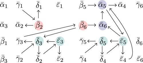
Figure 18. The seed $\Sigma_{D}$ associated to the chord diagram $D$ above (also in Figure 15). The variables $\mathbf{x}(D)$ are as in Example 8.5. The mutable variables $\operatorname{Mut}(Z_{D})$ are circled; the other variables are the frozen variables $\operatorname{Froz}(Z_{D})$. The colors (red, green, blue) indicate the different cases of Definition 9.8.

Example 9.9 (Seed of a standard BCFW tile).

The seed $\Sigma_{D}$ from Figure 18 is built from Definition 9.8 by applying the rules for the following conditions. Head-to-tail left siblings: $(i,j)\in\{(2,1),(6,3)\}$; same-end child: $(i,j)\in\{(3,2),(5,4)\}$; sticky child: $(i,j)\in\{(6,5),(5,4)\}$.

Theorem 9.10 and Theorem 9.11 are the main results of this section. They will be proved in Section 9.3 and Section 9.4.

Theorem 9.10 (The seed of a standard BCFW tile is a subseed of a $\operatorname{Gr}_{4,n}$ seed).

Let $D\in\mathcal{CD}_{n,k}$. The seed $\Sigma_{D}=(\overline{\mathbf{x}}(D),Q_{D})$ is obtained from the seed $\widetilde{\Sigma}_{D}=(\widetilde{\mathbf{x}}(D),\widetilde{Q}_{D})$ for $\operatorname{Gr}_{4,n}$ by freezing the variables not in the set $\operatorname{Mut}(Z_{D})$ of Definition 9.8. Hence every cluster variable (respectively, exchange relation) of $\mathcal{A}(\Sigma_{D})$ is a cluster variable (resp., exchange relation) for $\operatorname{Gr}_{4,n}$.

The following theorem characterizes the open BCFW tile $Z_{D}^{\circ}$ in terms of any extended cluster of $\mathcal{A}(\Sigma_{D})$. It generalizes Corollary 7.12 for standard BCFW tiles.

Theorem 9.11 (Positivity tests for standard BCFW tiles).

Let $D\in\mathcal{CD}_{n,k}$. Using 7.11, every cluster and frozen variable $x$ in $\mathcal{A}(\Sigma_{D})$ is such that $x(Y)$ has a definite sign $s_{x}\in\{1,-1\}$ on the open BCFW tile $Z_{D}^{\circ}$, where the signs of the domino variables are given by Proposition 8.10. We have

$$Z_{D}^{\circ} =\{Y\in\operatorname{Gr}_{k,k+4}:s_{x}\cdot x(Y)>0\text{ for all }x\in\mathbf{x}(D)\}$$

$$=\{Y\in\operatorname{Gr}_{k,k+4}:s_{x}\cdot x(Y)>0\text{ for all }x\in\widetilde{\mathbf{x}}(D)\}$$

$$=\{Y\in\operatorname{Gr}_{k,k+4}:s_{x}\cdot x(Y)>0\text{ for all }x\text{ in any fixed extended cluster of }\mathcal{A}(\Sigma_{D})\}.$$

Example 9.12 (Positivity test for the standard BCFW tiles).

For the tile $Z_{D}$ with chord diagram $D$ in Figure 18, we have:

$$Z_{D}^{\circ}=\{Y\in\operatorname{Gr}_{6,10}:s_{x}\cdot x(Y)>0\text{ for all }x\in\mathbf{x}(D)\},$$

with $\mathbf{x}(D)$ as in Example 8.5 and the respective signs $s_{x}$ as in Example 8.11.

The following lemma provides a description of exchange relations which is equivalent to the local description given in Definition 9.8. Lemma 9.13 will be useful in the proof of Theorem 9.10.

Lemma 9.13.

Let $D\in\mathcal{CD}_{n,k}$. The exchange relations of $\Sigma_{D}$ are as follows.
R1. (Sticky) Suppose that $D_{i}$ is a chord with a sticky child $D_{j}$. Then

$$\bar{\alpha}_{i}\bar{\alpha}_{i}^{\prime}=(\bar{\beta}_{i})\bar{\varepsilon}_{j}(\bar{\alpha}_{p})+\bar{\alpha}_{j}(\bar{\varepsilon}_{i}),$$

where $\bar{\beta}_{i}$ appears unless $D_{i}$ has a sticky same-end parent, $\bar{\alpha}_{p}$ is present only if $D_{i}$ has a sticky parent $D_{p}$, and $\bar{\varepsilon}_{i}$ is present only if $D_{j}$ is same-end with $D_{i}$.

	$\bar{\alpha}_{i}\bar{\alpha}^{\prime}_{i}=\bar{\beta}_{i}\bar{\varepsilon}_{j}+\bar{\alpha}_{j}$	$\bar{\alpha}_{i}\bar{\alpha}^{\prime}_{i}=\bar{\beta}_{i}\bar{\varepsilon}_{j}+\bar{\alpha}_{j}\bar{\varepsilon}_{i}$
$\bar{\alpha}_{i}\bar{\alpha}^{\prime}_{i}=\bar{\beta}_{i}\bar{\varepsilon}_{j}\bar{\alpha}_{p}+\bar{\alpha}_{j}$	$\bar{\alpha}_{i}\bar{\alpha}^{\prime}_{i}=\bar{\beta}_{i}\bar{\varepsilon}_{j}\bar{\alpha}_{p}+\bar{\alpha}_{j}\bar{\varepsilon}_{i}$	$\bar{\alpha}_{i}\bar{\alpha}_{i}^{\prime}=\bar{\varepsilon}_{j}\bar{\alpha}_{p}+\bar{\alpha}_{j}$	$\bar{\alpha}_{i}\bar{\alpha}_{i}^{\prime}=\bar{\varepsilon}_{j}\bar{\alpha}_{p}+\bar{\alpha}_{j}\bar{\varepsilon}_{i}$

R2. (Head-to-tail) Suppose that $D_{i}$ has a head-to-tail sibling $D_{j}$ on its left. Then

$\bar{\beta}_{i}\bar{\beta}_{i}^{\prime}=\bar{\gamma}_{j}+\bar{\alpha}_{i}\bar{\delta}_{j}$

R3a. (Same end) Suppose that $D_{i}$ has a same-end child $D_{j}$. Then

$$\bar{\delta}_{i}\bar{\delta}_{i}^{\prime}=\bar{\gamma}_{j}\bar{\varepsilon}_{i}(\bar{\delta}_{p})(\bar{\beta}_{\ell})+\bar{\gamma}_{i}\bar{\delta}_{j}(\bar{\varepsilon}_{p}),$$

where $\bar{\delta}_{p}$ and $\bar{\varepsilon}_{p}$ are present only if $D_{i}$ has a same-end parent $D_{p}$ and $\bar{\beta}_{\ell}$ is present only if $D_{i}$ has a head-to-tail sibling $D_{\ell}$ to its right.

$\bar{\delta}_{i}\bar{\delta}^{\prime}_{i}=\bar{\gamma}_{j}\bar{\varepsilon}_{i}+\bar{\gamma}_{i}\bar{\delta}_{j}$	$\bar{\delta}_{i}\bar{\delta}^{\prime}_{i}=\bar{\gamma}_{j}\bar{\varepsilon}_{i}\bar{\beta}_{\ell}+\bar{\gamma}_{i}\bar{\delta}_{j}$	$\bar{\delta}_{i}\bar{\delta}^{\prime}_{i}=\bar{\gamma}_{j}\bar{\varepsilon}_{i}\bar{\delta}_{p}+\bar{\gamma}_{i}\bar{\delta}_{j}\bar{\varepsilon}_{p}$

R3b. (Same end) Suppose that $D_{i}$ has a same-end child $D_{j}$. Then

$$\bar{\varepsilon}_{i}\bar{\varepsilon}_{i}^{\prime}=\bar{\delta}_{j}(\bar{\alpha}_{i})(\bar{\varepsilon}_{p})+\bar{\delta}_{i}\bar{\varepsilon}_{j}(\bar{\alpha}_{p}),$$

where $\bar{\alpha}_{i}$ is present only if $D_{j}$ is sticky to $D_{i}$, $\bar{\varepsilon}_{p}$ is present only if $D_{i}$ has a same-end parent $D_{p}$, and $\bar{\alpha}_{p}$ is present only if $D_{i}$ has a sticky parent $D_{p}$.

$\bar{\varepsilon}_{i}\bar{\varepsilon}^{\prime}_{i}=\bar{\delta}_{j}+\bar{\delta}_{i}\bar{\varepsilon}_{j}$	$\bar{\varepsilon}_{i}\bar{\varepsilon}^{\prime}_{i}=\bar{\delta}_{j}\bar{\alpha}_{i}+\bar{\delta}_{i}\bar{\varepsilon}_{j}$	$\bar{\varepsilon}_{i}\bar{\varepsilon}^{\prime}_{i}=\bar{\delta}_{j}\bar{\varepsilon}_{p}+\bar{\delta}_{i}\bar{\varepsilon}_{j}$	$\bar{\varepsilon}_{i}\bar{\varepsilon}^{\prime}_{i}=\bar{\delta}_{j}\bar{\alpha}_{i}\bar{\varepsilon}_{p}+\bar{\delta}_{i}\bar{\varepsilon}_{j}$
$\bar{\varepsilon}_{i}\bar{\varepsilon}^{\prime}_{i}=\bar{\delta}_{j}\bar{\varepsilon}_{p}+\bar{\delta}_{i}\bar{\varepsilon}_{j}\bar{\alpha}_{p}$	$\bar{\varepsilon}_{i}\bar{\varepsilon}^{\prime}_{i}=\bar{\delta}_{j}\bar{\alpha}_{i}\bar{\varepsilon}_{p}+\bar{\delta}_{i}\bar{\varepsilon}_{j}\bar{\alpha}_{p}$	$\bar{\varepsilon}_{i}\bar{\varepsilon}^{\prime}_{i}=\bar{\delta}_{j}+\bar{\delta}_{i}\bar{\varepsilon}_{j}\bar{\alpha}_{p}$	$\bar{\varepsilon}_{i}\bar{\varepsilon}^{\prime}_{i}=\bar{\delta}_{j}\bar{\alpha}_{i}+\bar{\delta}_{i}\bar{\varepsilon}_{j}\bar{\alpha}_{p}$

Example 9.14.

The exchange relations for $\Sigma_{D}$ in Figure 18 can be obtained from Lemma 9.13 as:

$$\mbox{R1. i), }(i,j)=(6,5):\bar{\alpha}^{\prime}_{6}\bar{\alpha}_{6}=\bar{\beta}_{6}\bar{\varepsilon}_{5}+\bar{\alpha}_{5},\quad\mbox{R1. iv), }(p,i,j)=(6,5,4):\bar{\alpha}^{\prime}_{5}\bar{\alpha}_{5}=\bar{\beta}_{5}\bar{\varepsilon}_{4}\bar{\alpha}_{6}+\bar{\alpha}_{5}\bar{\varepsilon}_{5}.$$

$$\mbox{R2, }(i,j)=(2,1):\bar{\beta}^{\prime}_{2}\bar{\beta}_{2}=\bar{\gamma}_{1}+\bar{\alpha}_{2}\bar{\delta}_{1},\quad\mbox{R2, }(i,j)=(6,3):\bar{\beta}^{\prime}_{6}\bar{\beta}_{6}=\bar{\gamma}_{3}+\bar{\alpha}_{6}\bar{\delta}_{3}.$$

$$\mbox{R3a ii), }(i,j,\ell)=(3,2,6):\bar{\delta}^{\prime}_{3}\bar{\delta}_{3}=\bar{\gamma}_{2}\bar{\varepsilon}_{3}\bar{\beta}_{6}+\bar{\gamma}_{3}\bar{\delta}_{2},\quad\mbox{R3a i), }(i,j)=(5,4):\bar{\delta}^{\prime}_{5}\bar{\delta}_{5}=\bar{\gamma}_{4}\bar{\varepsilon}_{3}+\bar{\gamma}_{3}\bar{\delta}_{2}.$$

$$\mbox{R3b i), }(i,j)=(3,2):\bar{\varepsilon}^{\prime}_{3}\bar{\varepsilon}_{3}=\bar{\delta}_{2}+\bar{\delta}_{3}\bar{\varepsilon}_{2},\quad\mbox{R3b viii), }(p,i,j)=(6,5,4):\bar{\varepsilon}^{\prime}_{5}\bar{\varepsilon}_{5}=\bar{\delta}_{4}\bar{\alpha}_{5}+\bar{\delta}_{5}\bar{\varepsilon}_{4}\bar{\alpha}_{6}.$$

See Example 9.16 for expressions of the primed variables and Example 8.5 for the non-primed ones.

9.2. Cluster variables obtained from $\Sigma_{D}$ by a single mutation

There are several ways to show that the cluster variables in $\mathcal{A}(\Sigma(D))$ are regular on $\operatorname{Gr}_{4,n}$. One way is to show that the cluster variables obtained by any single mutation of the initial seed are regular functions on $\operatorname{Gr}_{4,n}$ (then use the Starfish lemma [FWZa, Proposition 6.4.1]). We do this in Proposition 9.15, which gives explicit formulas for these cluster variables as polynomials in Plücker coordinates. We give a second way in the proof of Theorem 9.10, which proves the stronger statement that each exchange relation in $\mathcal{A}(\Sigma(D))$ is in fact an exchange relation in the cluster structure for $\operatorname{Gr}_{4,n}$.

Proposition 9.15.

Let $D\in\mathcal{CD}_{n,k}$, and let $\bar{\alpha}^{\prime}_{i},\bar{\beta}^{\prime}_{i},\bar{\delta}^{\prime}_{i},\bar{\varepsilon}^{\prime}_{i}$ be as in Lemma 9.13. Then:

R1. $\bar{\alpha}_{i}^{\prime}=\langle a_{i},b_{i}+1,c_{j},d_{j}\rangle$.

R2. $\bar{\beta}_{i}^{\prime}=\langle a_{j},b_{j},b_{i}\operatorname{\widetilde{\nearrow}}_{j}n\rangle$.

• R3a. i) $\bar{\beta}_{\ell},\bar{\delta}_{p},\bar{\epsilon}_{p}$ are not present: $\bar{\delta}_{i}^{\prime}=\begin{cases}\langle a_{i}\,b_{i}\,d_{i}|a_{j}\,b_{j}|c_{i}\,d_{i}\nearrow_{j}n\rangle&\text{if $D_{j}$ not sticky}\\ \langle a^{\prime}_{j},a_{j},b_{j},d_{i}\rangle&\text{if $D_{j}$ sticky}\end{cases}$

• ii) $\bar{\beta}_{\ell}$ is present: $\bar{\delta}_{i}^{\prime}=\langle n\operatorname{\widetilde{\nwarrow}}_{j}\,a_{j}\,b_{j}|a_{\ell}\,b_{\ell}|c_{\ell}\,d_{\ell}\nearrow_{\ell}n\rangle$.

• iii) $\bar{\delta}_{p},\bar{\varepsilon}_{p}$ are present: $\bar{\delta}_{i}^{\prime}=\langle n\operatorname{\widetilde{\nwarrow}}_{p}\,a_{p}\,b_{p}|c_{i}\,d_{i}|b_{j}\,a_{j}\operatorname{\widetilde{\nearrow}}_{j}n\rangle$.

R3b. $\bar{\varepsilon}^{\prime}_{i}=\langle a_{j},b_{j},c_{i},\nearrow_{i}n\rangle$.

Example 9.16.

The variables $\bar{\alpha}^{\prime}_{i},\bar{\beta}^{\prime}_{i},\bar{\delta}^{\prime}_{i},\bar{\varepsilon}^{\prime}_{i}$ in Proposition 9.15 for Figure 15 are as follows. See also Example 9.14 for the corresponding exchange relations. We will denote $(10,\ldots,15)$ as $(A,\ldots,F)$.

$$\mbox{R1. i), }(i,j)=(6,5):\bar{\alpha}^{\prime}_{6}=\langle 8\,A\,C\,D\rangle,\quad\mbox{R1. iv), }(p,i,j)=(6,5,4):\bar{\alpha}^{\prime}_{5}=\langle 9\,B\,C\,D\rangle.$$

For rule R2, we have the pairs $(i,j)\in\{(2,1),(6,3)\}$, which gives respectively:

$$\bar{\beta}^{\prime}_{2}=\langle 3\,4\,6\operatorname{\widetilde{\nearrow}}_{1}F\rangle=\langle 3\,4\,6|2\,1|8\,9\,F\rangle,\quad\bar{\beta}^{\prime}_{6}=\langle 1\,2\,9\operatorname{\widetilde{\nearrow}}_{3}F\rangle=\langle 1\,2\,9\,F\rangle.$$

$$\mbox{R3a ii), }(i,j,\ell)=(3,2,6):\bar{\delta}^{\prime}_{3}=\langle F\operatorname{\widetilde{\nwarrow}}_{2}5\,6|8\,9|D\,E\nearrow_{6}F\rangle=\langle F\,8\,9|6\,5|8\,9|D\,E\,F\rangle.$$

$$\mbox{R3a i), }(i,j)=(5,4):\bar{\delta}^{\prime}_{5}=\langle 9\,A\,B\,D\rangle.$$

Finally, for rule R3b, we have the pairs $(i,j)\in\{(3,2),(5,4)\}$, which gives respectively:

$$\bar{\varepsilon}^{\prime}_{3}=\langle 5\,6\,8\nearrow_{3}F\rangle=\langle 5\,6\,8\,F\rangle,\quad\bar{\varepsilon}^{\prime}_{5}=\langle A\,B\,C\nearrow_{5}F\rangle=\langle A\,B\,C|9\,8|D\,E\,F\rangle.$$

In the following proof, we will use the following identities:

Lemma 9.17.

Let $a,b,c,d,e,x,y,z\in[n]$, then

• $\langle n\operatorname{\widetilde{\nwarrow}}_{a}b\,c\,d\rangle=-\langle b\,c\,d\operatorname{\widetilde{\nearrow}}_{a}n\rangle$;

• $\langle x\,y\,z\,a\rangle\langle b\,c\,d\,e\rangle=\langle x\,y\,z\,b\rangle\langle a\,c\,d\,e\rangle-\langle x\,y\,z\,c\rangle\langle a\,b\,d\,e\rangle+\langle x\,y\,z\,d\rangle\langle a\,b\,c\,e\rangle-\langle x\,y\,z\,e\rangle\langle a\,b\,c\,d\rangle$, and we will say we used the Plücker identity for the five marked vectors in $\langle x\,y\,z\,\underline{a}\rangle\langle\underline{b}\,\underline{c}\,\underline{d}\,\underline{e}\rangle$.

Proof of Proposition 9.15.

We will provide detailed proofs of Cases (R1) and (R2), below. Case (R3) can be proved in a similar fashion.

Case R1. i) $D_{i}$ has a sticky not same-end child $D_{j}$. $D_{i}$ is not a sticky child.

In this case, the exchange relation is

$$\bar{\alpha}_{i}\bar{\alpha}_{i}^{\prime}=\bar{\beta}_{i}\bar{\varepsilon}_{j}+\bar{\alpha}_{j},$$

moreover $(a_{i},b_{i},b_{i}+1)=(a^{\prime}_{j},a_{j},b_{j})$. Then

$$\bar{\alpha}_{j}=\langle b_{j},c_{j},d_{j}\nearrow_{j}n\rangle=\langle b_{i}+1,c_{j},d_{j}\nearrow_{j}n\rangle=\langle b_{i}+1,c_{j},d_{j}|b_{i}\,a_{i}|c_{i}\,d_{i}\nearrow_{i}n\rangle,$$

as $|c_{j},d_{j}\nearrow_{j}n\rangle=|c_{j},d_{j}|b_{i}\,a_{i}|c_{i}\,d_{i}\nearrow_{i}n\rangle$, in this case. From expanding the chain polynomial above:

$$\bar{\alpha}_{j}=\underbrace{\langle b_{i}+1,c_{j},d_{j}\,b_{i}\rangle}_{-\bar{\varepsilon}_{j}}\underbrace{\langle a_{i}\,c_{i}\,d_{i}\nearrow_{i}n\rangle}_{\bar{\beta}_{i}}-\underbrace{\langle b_{i}+1,c_{j},d_{j}\,a_{i}\rangle}_{-\bar{\alpha}^{\prime}_{i}}\underbrace{\langle b_{i}\,c_{i}\,d_{i}\nearrow_{i}n\rangle}_{\bar{\alpha}_{i}}.$$

Case R1. ii) $D_{i}$ is not a sticky child and it has a sticky same-end child $D_{j}$. In this case, the exchange relation is

$$\bar{\alpha}_{i}\bar{\alpha}_{i}^{\prime}=\bar{\beta}_{i}\bar{\varepsilon}_{j}+\bar{\alpha}_{j}\bar{\varepsilon}_{i},$$

moreover $(a_{i},b_{i},b_{i}+1,c_{i},d_{i})=(a^{\prime}_{j},a_{j},b_{j},c_{j},d_{j})$. Then

$$\underbrace{\langle a_{i}\,c_{i}\,d_{i}\nearrow_{i}n\rangle}_{\bar{\beta}_{i}}\underbrace{\langle b_{i},b_{i}+1,c_{i},d_{i}\rangle}_{\bar{\varepsilon}_{j}}+\underbrace{\langle b_{i}+1,c_{i},d_{i}\nearrow_{j}n\rangle}_{\bar{\alpha}_{j}}\underbrace{\langle a_{i},b_{i},c_{i},d_{i}\rangle}_{\bar{\varepsilon}_{i}}=\underbrace{\langle b_{i}\,c_{i}\,d_{i}\nearrow_{j}n\rangle}_{\bar{\alpha}_{i}}\underbrace{\langle a_{i},b_{i}+1,c_{i},d_{i}\rangle}_{\bar{\alpha}^{\prime}_{i}},$$

where we used the Plücker identity for the $5$ highlighted vectors in $\langle\underline{a_{i}}\,c_{i}\,d_{i}\nearrow_{i}n\rangle\langle\underline{b_{i}},\underline{b_{i}+1},\underline{c_{i}},\underline{{d_{i}}}\rangle$, and $|c_{i},d_{i}\nearrow_{j}n\rangle=|c_{i},d_{i}\nearrow_{i}n\rangle$, in this case.

Case R1. iii) $D_{i}$ has a sticky non same-end child $D_{j}$ and a sticky non same-end parent $D_{p}$. In this case, the exchange relation is

$$\bar{\alpha}_{i}\bar{\alpha}_{i}^{\prime}=\bar{\beta}_{i}\bar{\varepsilon}_{j}\bar{\alpha}_{p}+\bar{\alpha}_{j},$$

moreover $(a_{p},b_{p})=(a^{\prime}_{i},a_{i})$ and $(a_{i},b_{i},b_{i}+1)=(a^{\prime}_{j},a_{j},b_{j})$. Then

$$\bar{\alpha}_{j}=\langle b_{j},c_{j},d_{j}\nearrow_{j}n\rangle=\langle b_{i}+1,c_{j},d_{j}\nearrow_{j}n\rangle=\langle b_{i}+1,c_{j},d_{j}|b_{i}\,a_{i}|c_{i}\,d_{i}|a_{i}\,a^{\prime}_{i}|c_{p}\,d_{p}\nearrow_{p}n\rangle,$$

as $|c_{j},d_{j}\nearrow_{j}n\rangle=|c_{j},d_{j}|b_{i}\,a_{i}|c_{i}\,d_{i}|b_{p}\,a_{p}|c_{p}\,d_{p}\nearrow_{p}n\rangle$, in this case. From expanding the chain polynomial above:

$$-\underbrace{\langle b_{i}+1,c_{j},d_{j},a_{i}\rangle}_{-\bar{\alpha}^{\prime}_{i}}\underbrace{\langle b_{i}\,c_{i}\,d_{i}|a_{i}\,a^{\prime}_{i}|c_{p}\,d_{p}\nearrow_{p}n\rangle}_{\bar{\alpha}_{i}}-\underbrace{\langle b_{i}+1,c_{j},d_{j},b_{i}\rangle}_{-\bar{\varepsilon}_{j}}\underbrace{\langle a_{i}\,c_{i}\,d_{i}\,a^{\prime}_{i}\rangle}_{-\bar{\beta}_{i}}\underbrace{\langle a_{i}\,c_{p}\,d_{p}\nearrow_{p}n\rangle}_{\bar{\alpha}_{p}},$$

as $|c_{i},d_{i}|a^{\prime}_{i}\,a_{i}|c_{p}\,d_{p}\nearrow_{p}n\rangle=|c_{i}\,d_{i}\nearrow_{i}n\rangle$, in this case.

Case R1. iv) $D_{i}$ has a sticky same-end child $D_{j}$ and a sticky non same-end parent $D_{p}$. In this case, the exchange relation is

$$\bar{\alpha}_{i}\bar{\alpha}_{i}^{\prime}=\bar{\beta}_{i}\bar{\varepsilon}_{j}\bar{\alpha}_{p}+\bar{\alpha}_{j}\bar{\varepsilon}_{i},$$

moreover $(a_{p},b_{p})=(a^{\prime}_{i},a_{i}),(a_{i},b_{i},b_{i}+1)=(a^{\prime}_{j},a_{j},b_{j})$ and $(c_{j},d_{j})=(c_{i},d_{i})$. Then

$$\underbrace{\langle b_{i}+1,c_{i},d_{i}|a_{i}\,a^{\prime}_{i}|c_{p}\,d_{p}\nearrow_{p}n\rangle}_{\bar{\alpha}_{j}}\underbrace{\langle a_{i},b_{i},c_{i},d_{i}\rangle}_{\bar{\varepsilon}_{i}}=$$

$$= \langle a_{i},c_{i},d_{i}|a_{i}\,a^{\prime}_{i}|c_{p}\,d_{p}\nearrow_{p}n\rangle\underbrace{\langle b_{i}+1,b_{i},c_{i},d_{i}\rangle}_{-\bar{\varepsilon}_{j}}-\underbrace{\langle b_{i},c_{i},d_{i}|a_{i}\,a^{\prime}_{i}|c_{p}\,d_{p}\nearrow_{p}n\rangle}_{\bar{\alpha}_{i}}\underbrace{\langle b_{i}+1,a_{i},c_{i},d_{i}\rangle}_{-\bar{\alpha}^{\prime}_{i}},$$

where we used the Plücker identity for the $5$ marked vectors in $\langle\underline{b_{i}+1},c_{i},d_{i}|a_{i}\,a^{\prime}_{i}|c_{p}\,d_{p}\nearrow_{p}n\rangle\langle\underline{a_{i}},\underline{b_{i}},\underline{c_{i}},\underline{d_{i}}\rangle$ and $|c_{i},d_{i}|a_{i}\,a^{\prime}_{i}|c_{p}\,d_{p}\nearrow_{p}n\rangle=|c_{i},d_{i}|b_{p}\,a_{p}|c_{p}\,d_{p}\nearrow_{p}n\rangle=|c_{i},d_{i}\nearrow_{i}n\rangle$. Finally, we have:

$$\langle a_{i},c_{i},d_{i}|a_{i}\,a^{\prime}_{i}|c_{p}\,d_{p}\nearrow_{p}n\rangle=\langle a^{\prime}_{i}\,a_{i}\,d_{i}|a_{i}\,c_{i}|c_{i}\,d_{i}\nearrow_{p}n\rangle=-\underbrace{\langle a^{\prime}_{i}\,a_{i}\,d_{i}\,c_{i}\rangle}_{\bar{\beta}_{i}}\underbrace{\langle a_{i}\,c_{i}\,d_{i}\nearrow_{p}n\rangle}_{\bar{\alpha}_{p}}.$$

Case R1. v) $D_{i}$ has a sticky non same-end child $D_{j}$ and a sticky same-end parent $D_{p}$. In this case, the exchange relation is

$$\bar{\alpha}_{i}\bar{\alpha}_{i}^{\prime}=\bar{\varepsilon}_{j}\bar{\alpha}_{p}+\bar{\alpha}_{j},$$

moreover $(a_{p},b_{p})=(a^{\prime}_{i},a_{i})$ and $(a_{i},b_{i},b_{i}+1,c_{i},d_{i})=(a^{\prime}_{j},a_{j},b_{j},c_{j},d_{j})$. Then

$$\bar{\alpha}_{j}=\langle b_{j},c_{j},d_{j}\nearrow_{j}n\rangle=\langle b_{i}+1,c_{j},d_{j}|b_{i}\,a_{i}|c_{i}\,d_{i}\nearrow_{p}\rangle,$$

as $|c_{j},d_{j}\nearrow_{j}n\rangle=|c_{j},d_{j}|b_{i}\,a_{i}|c_{i}\,d_{i}\nearrow_{p}n\rangle$, in this case. From expanding the chain polynomial above:

$$\underbrace{\langle b_{i}+1,c_{j},d_{j}\,b_{i}\rangle}_{-\bar{\varepsilon}_{j}}\underbrace{\langle a_{i}\,c_{i}\,d_{i}\nearrow_{p}n\rangle}_{\bar{\alpha}_{p}}-\underbrace{\langle b_{i}+1,c_{j},d_{j}\,a_{i}\rangle}_{-\bar{\alpha}^{\prime}_{i}}\underbrace{\langle b_{i}\,c_{i}\,d_{i}\nearrow_{p}n\rangle}_{\bar{\alpha}_{i}},$$

as $\nearrow_{p}n$ equals $\nearrow_{i}n$, in this case.

Case R1. vi) $D_{i}$ has a sticky same-end child $D_{j}$ and a sticky same-end parent $D_{p}$. In this case, the exchange relation is

$$\bar{\alpha}_{i}\bar{\alpha}_{i}^{\prime}=\bar{\varepsilon}_{j}\bar{\alpha}_{p}+\bar{\alpha}_{j}\bar{\varepsilon}_{i},$$

moreover $(a_{p},b_{p})=(a^{\prime}_{i},a_{i}),(a_{i},b_{i},b_{i}+1)=(a^{\prime}_{j},a_{j},b_{j})$ and $(c_{p},d_{p})=(c_{j},d_{j})=(c_{i},d_{i})$. Then

$$\underbrace{\langle b_{i}+1,c_{i},d_{i}\nearrow_{p}n\rangle}_{\bar{\alpha}_{j}}\underbrace{\langle a_{i}\,b_{i}\,c_{i}\,d_{i}\rangle}_{\bar{\varepsilon}_{i}}=\underbrace{\langle a_{i},c_{i},d_{i}\nearrow_{p}n\rangle}_{\bar{\alpha}_{p}}\underbrace{\langle b_{i}+1,b_{i},c_{i},d_{i}\rangle}_{-\bar{\varepsilon}_{j}}-\underbrace{\langle b_{i},c_{i},d_{i}\nearrow_{p}n\rangle}_{\bar{\alpha}_{i}}\underbrace{\langle b_{i}+1,a_{i},c_{i},d_{i}\rangle}_{-\bar{\alpha}^{\prime}_{i}},$$

where we used the Plücker identity on the $5$ highlighted vectors in $\langle\underline{b_{i}+1},c_{i},d_{i}\nearrow_{p}n\rangle\langle\underline{a_{i}}\,\underline{b_{i}}\,\underline{c_{i}}\,\underline{d_{i}}\rangle$ and used the fact that $|\ldots\nearrow_{p}n\rangle,|\ldots\nearrow_{i}n\rangle,|\ldots\nearrow_{j}n\rangle$ are all equal, in this case.

Case R2. $D_{i}$ has a head-to-tail sibling $D_{j}$ on its left. In this case, the exchange relation is

$$\bar{\beta}_{i}\bar{\beta}_{i}^{\prime}=\bar{\gamma}_{j}+\bar{\alpha}_{i}\bar{\delta}_{j},$$

moreover $(c_{j},d_{j})=(a_{i},b_{i})$. Then, expanding the following chain polynomial

$$\underbrace{\langle n\operatorname{\widetilde{\nwarrow}}_{j}\,a_{j}\,b_{j}|a_{i}\,b_{i}|c_{i}\,d_{i}\nearrow_{i}n\rangle}_{\bar{\gamma}_{j}}=\underbrace{\langle n\operatorname{\widetilde{\nwarrow}}_{j}\,a_{j}\,b_{j}\,a_{i}\rangle}_{-\bar{\delta}_{j}}\underbrace{\langle b_{i}\,c_{i}\,d_{i}\nearrow_{i}n\rangle}_{\bar{\alpha}_{i}}-\underbrace{\langle n\operatorname{\widetilde{\nwarrow}}_{j}\,a_{j}\,b_{j}\,b_{i}\rangle}_{-\bar{\beta}^{\prime}_{i}}\underbrace{\langle a_{i}\,c_{i}\,d_{i}\nearrow_{i}n\rangle}_{\bar{\beta}_{i}},$$

as $\operatorname{\widetilde{\nearrow}}_{i}$ equals $\nearrow_{i}$ in this case, and $\langle n\operatorname{\widetilde{\nwarrow}}_{j}\,a_{j}\,b_{j}\,x\rangle=-\langle a_{j}\,b_{j}\,x\operatorname{\widetilde{\nearrow}}_{j}n\rangle$.

∎

9.3. The proof of Theorem 9.10

We next turn to the proof of Theorem 9.10. In what follows, we say that a relation $xx^{\prime}=M+M^{\prime}$ is an exchange relation for $\operatorname{Gr}_{4,n}$ if there is a seed $\Sigma$ for $\operatorname{Gr}_{4,n}$ such that $xx^{\prime}=M+M^{\prime}$ is the exchange relation of $x$ in $\Sigma$.

As a first step towards proving Theorem 9.10, we prove the following lemma.

Lemma 9.18.

Suppose $D_{i}=(a_{i},b_{i},c_{i},d_{i})$ is the rightmost top chord of $D$. Then every exchange relation in Lemma 9.13 is an exchange relation for $\operatorname{Gr}_{4,n}$. In particular, in this case, the relations become the following:

1. (Sticky, not same-end) Suppose $D_{j}=(b_{i},b_{j},c_{j},d_{j})$ where $d_{j}<c_{i}$ is a sticky child of $D_{i}$. Then

   $$\underbrace{\langle b_{i}c_{i}d_{i}n\rangle}_{\bar{\alpha}_{i}}\underbrace{\langle a_{i}b_{j}c_{j}d_{j}\rangle}_{\bar{\alpha}_{i}^{\prime}}=\underbrace{\langle a_{i}c_{i}d_{i}n\rangle}_{\bar{\beta}_{i}}\underbrace{\langle b_{i}b_{j}c_{j}d_{j}\rangle}_{\bar{\varepsilon}_{j}}+\underbrace{\langle b_{j}c_{j}d_{j}\,|\,b_{i}a_{i}\,|\,c_{i}d_{i}n\rangle}_{\bar{\alpha}_{j}}.$$

2. (Sticky same-end) Suppose $D_{j}=(b_{i},b_{j},c_{i},d_{i})$ is a sticky same-end child of $D_{i}$. Then

   $$\underbrace{\langle b_{i}c_{i}d_{i}n\rangle}_{\bar{\alpha}_{i}}\underbrace{\langle a_{i}b_{j}c_{i}d_{i}\rangle}_{\bar{\alpha}_{i}^{\prime}}=\underbrace{\langle a_{i}c_{i}d_{i}n\rangle}_{\bar{\beta}_{i}}\underbrace{\langle b_{i}b_{j}c_{i}d_{i}\rangle}_{\bar{\varepsilon}_{j}}+\underbrace{\langle b_{j}c_{i}d_{i}n\rangle}_{\bar{\alpha}_{j}}\underbrace{\langle a_{i}b_{i}c_{i}d_{i}\rangle}_{\bar{\varepsilon}_{i}}.$$

3. (Head-to-tail) Suppose $D_{j}=(a_{j},b_{j},a_{i},b_{i})$ is a head-to-tail sibling of $D_{i}$ to its left. Then

   $$\underbrace{\langle a_{i}c_{i}d_{i}n\rangle}_{\bar{\beta}_{i}}\underbrace{\langle a_{j}b_{j}b_{i}n\rangle}_{\bar{\beta}_{i}^{\prime}}=\underbrace{\langle a_{j}b_{j}n\,|\,a_{i}b_{i}\,|\,c_{i}d_{i}n\rangle}_{\bar{\gamma}_{j}}+\underbrace{\langle b_{i}c_{i}d_{i}n\rangle}_{\bar{\alpha}_{i}}\underbrace{\langle a_{j}b_{j}a_{i}n\rangle}_{\bar{\delta}_{j}}.$$

4. (Same end, not sticky) Suppose that $D_{j}=(a_{j},b_{j},c_{i},d_{i})$ is a same-end nonsticky child of $D_{i}$ (so $b_{i}<a_{j}$). Then

   $$\underbrace{\langle a_{i}b_{i}c_{i}n\rangle}_{\bar{\delta}_{i}}\underbrace{\langle a_{j}b_{j}d_{i}\,|\,a_{i}b_{i}\,|\,c_{i}d_{i}n\rangle}_{\bar{\delta}_{i}^{\prime}}=\underbrace{\langle a_{j}b_{j}n\,|\,c_{i}d_{i}\,|\,a_{i}b_{i}n\rangle}_{\bar{\gamma}_{j}}\underbrace{\langle a_{i}b_{i}c_{i}d_{i}\rangle}_{\bar{\varepsilon}_{i}}+\underbrace{\langle a_{i}b_{i}d_{i}n\rangle}_{\bar{\gamma}_{i}}\underbrace{\langle a_{j}b_{j}c_{i}\,|\,b_{i}a_{i}\,|\,c_{i}d_{i}n\rangle}_{\bar{\delta}_{j}}.$$

5. (Same end sticky) Suppose $D_{j}=(b_{i},b_{j},c_{i},d_{i})$ is a sticky same-end child of $D_{i}$. Then

   $$\underbrace{\langle a_{i}b_{i}c_{i}n\rangle}_{\bar{\delta}_{i}}\underbrace{\langle a_{i}b_{i}b_{j}d_{i}\rangle}_{\bar{\delta}_{i}^{\prime}}=\underbrace{\langle a_{i}b_{i}b_{j}n\rangle}_{\bar{\gamma}_{j}}\underbrace{\langle a_{i}b_{i}c_{i}d_{i}\rangle}_{\bar{\varepsilon}_{i}}+\underbrace{\langle a_{i}b_{i}d_{i}n\rangle}_{\bar{\gamma}_{i}}\underbrace{\langle a_{i}b_{i}b_{j}c_{j}\rangle}_{\bar{\delta}_{j}}.$$

6. (Same end, not sticky) Suppose $D_{j}=(a_{j},b_{j},c_{i},d_{i})$ is a same-end nonsticky child of $D_{i}$. Then

   $$\underbrace{\langle a_{i}b_{i}c_{i}d_{i}\rangle}_{\bar{\varepsilon}_{i}}\underbrace{\langle a_{j}b_{j}c_{i}n\rangle}_{\bar{\varepsilon}_{i}^{\prime}}=\underbrace{\langle a_{j}b_{j}c_{i}\,|\,b_{i}a_{i}\,|\,c_{i}d_{i}n\rangle}_{\bar{\delta}_{j}}+\underbrace{\langle a_{i}b_{i}c_{i}n\rangle}_{\bar{\delta}_{i}}\underbrace{\langle a_{j}b_{j}c_{i}d_{i}\rangle}_{\bar{\varepsilon}_{j}}.$$

7. (Same end sticky) Suppose $D_{j}=(b_{i},b_{j},c_{i},d_{i})$ is a sticky same-end child of $D_{i}$. Then

   $$\underbrace{\langle a_{i}b_{i}c_{i}d_{i}\rangle}_{\bar{\varepsilon}_{i}}\underbrace{\langle b_{i}b_{j}c_{i}n\rangle}_{\bar{\varepsilon}_{i}^{\prime}}=\underbrace{\langle a_{i}b_{i}b_{j}c_{i}\rangle}_{\bar{\delta}_{j}}\underbrace{\langle b_{i}c_{i}d_{i}n\rangle}_{\bar{\alpha}_{i}}+\underbrace{\langle a_{i}b_{i}c_{i}n\rangle}_{\bar{\delta}_{i}}\underbrace{\langle b_{i}b_{j}c_{i}d_{i}\rangle}_{\bar{\varepsilon}_{j}}.$$

Proof.

Let $N$ be the set of 7 indices appearing in the domino variables of $D_{i},D_{j}$. One can check computationally that the relations listed are exchange relations for $\operatorname{Gr}_{4,N}\cong\operatorname{Gr}_{4,7}$, for example by searching through all seeds. Using Lemma 3.20, this shows that the relations are exchange relations for $\operatorname{Gr}_{4,n}$ for any $[n]\supset N$. ∎

Definition 9.19.

Let $D\in\mathcal{CD}_{n,k}$ be a chord diagram with rightmost top chord $D_{\operatorname{{\it k}}}=(a,b,c,d)$ and let $D_{L},D_{R}$ be as in Definition 8.1.

Let $R$ be a relation from Definition 9.8 for $\tilde{D}$, where $\tilde{D}=D_{L}$ or $\tilde{D}=D_{R}$ and suppose it is an exchange relation for $\operatorname{Gr}_{4,n}$. We say that $R$ is stable under promotion (induced by $D_{\operatorname{{\it k}}}$) if relation $R$ with the corresponding domino variables of $D$ is also an exchange relation for $\operatorname{Gr}_{4,n}$.

For example, if

(20) $$\bar{\beta}_{i}^{\tilde{D}}(\bar{\beta}_{i}^{\tilde{D}})^{\prime}=\bar{\gamma}_{j}^{\tilde{D}}+\bar{\alpha}_{i}^{\tilde{D}}\bar{\delta}_{j}^{\tilde{D}}$$

is an exchange relation for $\operatorname{Gr}_{4,n}$ and

$$\bar{\beta}_{i}^{{D}}(\bar{\beta}_{i}^{{D}})^{\prime}=\bar{\gamma}_{j}^{{D}}+\bar{\alpha}_{i}^{{D}}\bar{\delta}_{j}^{{D}}$$

is as well, then we say (20) is stable under promotion (induced by $D_{\operatorname{{\it k}}}$).

Proposition 9.20.

Let $D$ be a chord diagram on $[n]$. The relations (R1), (R2), (R3a) and (R3b) in Lemma 9.13 are exchange relations for $\operatorname{Gr}_{4,n}$.

Proof.

We will verify this using promotion. Because promotion is a quasi-cluster homomorphism (Theorem 4.7), we can obtain exchange relations for $\operatorname{Gr}_{4,n}$ by promoting exchange relations for $\operatorname{Gr}_{4,N_{L}}$ and $\operatorname{Gr}_{4,N_{R}}$. Using the notation of Theorem 4.7, let $x$ be a mutable variable of $\mathcal{A}(\Sigma_{0})$ in a seed $\Sigma$ and $u$ the corresponding cluster variable of $\mathcal{A}(\operatorname{Fr}(\Sigma_{1}))$ in a seed $\Sigma^{\prime}$ (which is also a seed for $\operatorname{Gr}_{4,n}$). If $xx^{\prime}=M+M$ is the exchange relation for $x$ in $\Sigma$ and $uu^{\prime}=N+N$ is the exchange relation in $\Sigma^{\prime}$, then $\Psi_{ac}(M+M^{\prime})$ differs from $N+N^{\prime}$ by a Laurent monomial in $\mathcal{T^{\prime}}$. To clear this monomial, we write $\Psi_{ac}(M+M^{\prime})$ over a common denominator, then take the numerator and remove all common factors in $\mathcal{T^{\prime}}$. Call the resulting binomial $f_{ac}(\Psi_{ac}(M+M^{\prime}))$; it is equal to $N+N^{\prime}$.

Consider a chord $D_{i}$ in $D$. By repeatedly removing penultimate markers which are not in any chord or removing the rightmost top chord and taking either $D_{L}$ or $D_{R}$ (defined as in Theorem 9.1), we obtain a chord diagram $D^{\prime}$ where $D_{i}$ is the rightmost top chord. Suppose the rightmost top chords we removed in this process were, in order, $(a_{1},b_{1},c_{1},d_{1}),\dots,(a_{p},b_{p},c_{p},d_{p})$. Using Lemma 8.7, we will show that each relation in Definition 9.8 is obtained from an exchange relation in Lemma 9.18 by the sequence $f_{a_{1}c_{1}}\circ\Psi_{a_{1}c_{1}}\circ\dots\circ f_{a_{p}c_{p}}\circ\Psi_{a_{p}c_{p}}$. By the previous paragraph, this will imply each relation in Definition 9.8 is an exchange relation for $\operatorname{Gr}_{4,n}$.

The following observation will be useful. It follows immediately from the definition of promotion.

Observation 9.21.

Suppose $D$ is a chord diagram on $N$ with largest markers $x,y:=x+1,n$ and choose $a,c$ such that $a<c-1,c<n-1$ and either $x\leq a$ or $a+1\leq x\leq c$. Let $M,M^{\prime}$ be any monomials in the domino variables of $D$ with no clauses containing $y$ but not $x$, the same number of clauses containing both $y$ and $n$, and the same number of clauses with $n$ but not $y$. Then the denominators of $\Psi_{ac}(M)$ and $\Psi_{ac}(M^{\prime})$ are equal.

[Case (R2.)] Suppose that $D_{i}$ and $D_{j}$ are chords which are head-to-tail siblings, with $D_{j}$ to the left of $D_{i}$. Since $D_{i}$ is a rightmost top chord in $D^{\prime}$, Lemma 9.18 implies that

(21) $$\bar{\beta}_{i}^{D^{\prime}}(\bar{\beta}_{i}^{D^{\prime}})^{\prime}=\bar{\gamma}_{j}^{D^{\prime}}+\bar{\alpha}_{i}^{D^{\prime}}\bar{\delta}_{j}^{D^{\prime}}\quad\text{or}\quad\langle a_{i}c_{i}d_{i}n\rangle(\bar{\beta}_{i}^{D^{\prime}})^{\prime}=\langle na_{j}b_{j}\,|\,a_{i}b_{i}\,|\,c_{i}d_{i}n\rangle+\langle b_{i}c_{i}d_{i}n\rangle\langle a_{j}b_{j}a_{i}n\rangle$$

is an exchange relation for $\operatorname{Gr}_{4,n}$. Now we show inductively that (21) is stable under the promotions $\Psi_{a_{p}c_{p}},\dots,\Psi_{a_{1}c_{1}}$. Suppose it is stable up until $\Psi=\Psi_{a_{q}c_{q}}$, corresponding to adding the rightmost top chord $D_{q}$. Let $\tilde{D}$ be the chord diagram obtained from $D^{\prime}$ by adding chords $D_{p},D_{p-1},\dots,D_{q+1}$ (and the appropriate chord diagrams beneath or to the left). By induction, (21) holds for $\tilde{D}$. Using Theorem 8.4, the terms on the right hand side satisfy the conditions of 9.21. More specifically, $\bar{\alpha}_{i}^{\tilde{D}}=\langle b_{i}c_{i}d_{i}\nearrow_{i}n\rangle$,

$$\bar{\gamma}_{j}^{\tilde{D}}=\begin{cases}\langle n\nwarrow_{j}a_{j}b_{j}\,|\,a_{i}b_{i}\,|\,c_{i}d_{i}\nearrow_{j}n\rangle&\text{$D_{j}$ not sticky}\\ \langle a_{j}a_{j}^{\prime}b_{j}\,|\,a_{i}b_{i}\,|\,c_{i}d_{i}\nearrow_{j}n\rangle&\text{$D_{j}$ sticky}\end{cases}\quad\text{and}\quad\bar{\delta}_{j}^{\tilde{D}}=\begin{cases}\langle a_{j}b_{j}a_{i}\nearrow_{j}n\rangle&\text{$D_{j}$ not sticky}\\ \langle a_{j}^{\prime}a_{j}b_{j}a_{i}\rangle&\text{$D_{j}$ sticky}\\ \end{cases}.$$

There are no clauses containing the penultimate marker $d$ of $\tilde{D}$ but not $d-1$. In $\bar{\gamma}_{j}^{\tilde{D}}$, the clause $\,|\,c_{i}d_{i}\nearrow_{j}n\rangle$ is equal to $\,|\,c_{i}d_{i}\nearrow_{i}n\rangle$ because $D_{j},D_{i}$ are siblings. Also, $b_{j}a_{i}\nearrow_{j}n$ in $\bar{\delta}_{j}^{\tilde{D}}$ involves the same chain of ancestors as $n\nwarrow_{j}a_{j}b_{j}$ in $\bar{\gamma}_{j}^{\tilde{D}}$, so if this chain is nontrivial, the end clause is the same in each. This verifies the conditions of 9.21.

So after promotion $\Psi_{a_{q}c_{q}}$, both terms have the same denominator. By Lemma 8.7, nontrivial factorization occurs in the numerator only if $D_{j}$ is a sticky child of $D_{q}$. In this case, the numerator of $\Psi(\bar{\gamma}_{j}^{\tilde{D}})$ is $\bar{\alpha}_{q}\bar{\gamma}_{j}$ and the numerator of $\Psi(\bar{\delta}_{j}^{\tilde{D}})$ is $\bar{\alpha}_{q}\bar{\delta}_{j}$, so $\bar{\alpha}_{q}$ is a common factor of the numerator. So applying $f_{a_{q}c_{q}}$ gives (21) for the chord diagram with $D_{q}$ added. Thus (21) is stable under promotion by $D_{q}$.

[Case (R3a.)] Suppose that $D_{i}$ is a same-end parent of $D_{j}$. Lemma 9.18 implies that

(22) $$\bar{\delta}_{i}^{D^{\prime}}(\bar{\delta}_{i}^{D^{\prime}})^{\prime}=\bar{\gamma}_{j}^{D^{\prime}}\bar{\varepsilon}_{i}^{D^{\prime}}+\bar{\gamma}_{i}^{D^{\prime}}\bar{\delta}_{j}^{D^{\prime}}$$

is an exchange relation for $\operatorname{Gr}_{4,n}$. It is straightforward to verify that (22) is stable under any sequence of promotions corresponding to chords which are not same-end parents or head-to-tail siblings with $D_{i}$. (Note that this implies none of the chords in the sequence are same-end or head-to-tail with $D_{i}$.) Indeed, using Theorem 8.4, the assumptions of 9.21 hold for each promotion in the sequence, so both terms of the right-hand side have the same denominator. There are no factorizations in the numerator unless the chord $D_{q}$ added is sticky to $D_{i}$. Then by Lemma 8.7, both $\Psi(\bar{\gamma}_{j})$ and $\Psi(\bar{\gamma}_{i})$ have a factor of $\bar{\alpha}_{p}$ and there are no other factorizations. So we see (22) is stable.

Now suppose one of the chords $D_{1},\dots,D_{p}$ is a same-end parent of $D_{i}$. This chord is necessarily $D_{p}$, so we are applying product promotion $\Psi=\Psi_{a_{p}c_{p}}$ to (22). The denominator of $\Psi(\bar{\gamma}_{j}^{D^{\prime}})$ is $\epsilon_{p}$, and the denominator of $\Psi(\bar{\gamma}_{i}^{D^{\prime}})$ is $\delta_{p}$; $\Psi$ fixes both $\bar{\delta}_{j}^{D^{\prime}}$ and $\bar{\varepsilon}_{i}^{D^{\prime}}$. If $D_{p}$ is not a sticky parent, then by Lemma 8.7, when we apply promotion to the right-hand side of (22), no extra factors will appear in the numerators. If $D_{p}$ is a sticky parent, then by Lemma 8.7 (1), the numerator of $\Psi(\bar{\gamma}_{i}^{D^{\prime}})$ is $\bar{\alpha}_{p}\bar{\gamma}_{i}^{D^{\prime\prime}}$; by Lemma 8.7 (3), the numerator of $\Psi(\bar{\gamma}_{j}^{D^{\prime}})$ is $\bar{\alpha}_{p}\bar{\gamma}_{j}^{D^{\prime\prime}}$; and no other factorizations occur. In either case, after applying $f_{a_{p}c_{p}}$, we obtain the exchange relation

(23) $$\bar{\delta}_{i}^{D^{\prime\prime}}(\bar{\delta}_{i}^{D^{\prime\prime}})^{\prime}=\bar{\gamma}_{j}^{D^{\prime\prime}}\bar{\varepsilon}_{i}^{D^{\prime\prime}}\bar{\delta}_{p}^{D^{\prime\prime}}+\bar{\gamma}_{i}^{D^{\prime\prime}}\bar{\delta}_{j}^{D^{\prime\prime}}\bar{\varepsilon}_{p}^{D^{\prime\prime}},$$

where $D^{\prime\prime}$ is the diagram obtained from $D^{\prime}$ by adding $D_{p}$ and chords to its left. Further, (23) is stable under all subsequent promotions, again using Theorem 8.4 to check 9.21 and Lemma 8.7 to check that any factorization in numerators contributes the same factor to each term.

Now suppose instead one of the chords $D_{1},\dots,D_{p}$ is a head-to-tail sibling with $D_{i}$ to its right. Again, this chord must be $D_{p}$. Note that $\Psi_{a_{p}c_{p}}$ acts nontrivially on a domino variable of (22) only if that domino variable has a clause containing $b_{r}=d_{i}$ but not $a_{r}=c_{i}$. Using Theorem 8.4, the only such domino variable of (22) is $\bar{\gamma}_{i}^{D^{\prime}}=\langle a_{i},b_{i},b_{p},n\rangle$, and hence when we apply promotion to $\bar{\gamma}_{i}^{D^{\prime}}$ we introduce a new denominator of $\beta_{p}$. There is no factorization in any numerators, so applying $f_{a_{p}c_{p}}$, we obtain

(24) $$\bar{\delta}_{i}^{D^{\prime\prime}}(\bar{\delta}_{i}^{D^{\prime\prime}})^{\prime}=\bar{\gamma}_{j}^{D^{\prime\prime}}\bar{\varepsilon}_{i}^{D^{\prime\prime}}\bar{\beta}_{p}^{D^{\prime\prime}}+\bar{\gamma}_{i}^{D^{\prime\prime}}\bar{\delta}_{j}^{D^{\prime\prime}},$$

where $D^{\prime\prime}$ is the chord diagram obtained from $D^{\prime}$ by adding $D_{p}$ and chords below it. The relation (24) is stable under all subsequent promotions, by a similar argument as previously.

The proofs of relations (R1) and (R3b) are similar to the proofs above, so we omit them. ∎

Proof of Theorem 9.10.

Let $D\in\mathcal{CD}_{n,k}$ and $\Sigma_{D}$ be the seed defined in Definition 9.8. By Theorem 9.1, $\widetilde{\mathbf{x}}(D)$ is an extended cluster for $\operatorname{Gr}_{4,n}$ and $\widetilde{\Sigma}_{D}=(\widetilde{\mathbf{x}}(D),\widetilde{Q}_{D})$ is the unique seed of $\operatorname{Gr}_{4,n}$ with that cluster. We need to show that for any $x\in\operatorname{Mut}(Z_{D})$, the exchange relation of $x$ is the same in $\Sigma_{D}$ and $\widetilde{\Sigma}_{D}$.

Recall that the mutable variables $\operatorname{Mut}(Z_{D})$ are precisely those appearing on the left hand side of relations (R1), (R2), (R3a), (R3b). Fix $x\in\operatorname{Mut}(Z_{D})$, let $R$ be its exchange relation in $\Sigma_{D}$, and let $U$ be all neighbors of $x$ in $\Sigma_{D}$. By Proposition 9.20, there is a seed $\Sigma^{\prime}$ of $\operatorname{Gr}_{4,n}$ containing $\{x\}\cup U$ and $R$ is the exchange relation of $x$ in $\Sigma^{\prime}$. Now, by [CL20, Theorem 10], any seed of $\operatorname{Gr}_{4,n}$ containing $\{x\}\cup U$ may be obtained from $\Sigma^{\prime}$ by a sequence of mutations avoiding $\{x\}\cup U$, and thus $x$ has exchange relation $R$ in any seed containing $\{x\}\cup U$. Since $\widetilde{\Sigma}_{D}$ contains $\{x\}\cup U$, $x$ also has exchange relation $R$ in $\widetilde{\Sigma}_{D}$. We have shown the first sentence of the theorem statement. The second sentence follows immediately. ∎

9.4. Signed seeds and the proof of Theorem 9.11

The following notion of signed seed will be useful for proving Theorem 9.11.

Definition 9.22 (Signed seed).

Given a seed $((x_{1},\dots,x_{s}),Q)$, let $(\sigma_{1},\dots,\sigma_{s})\in\{1,-1\}^{s}$ be an assignment of signs to each cluster and frozen variable. We denote the vertices of $Q$ by $v_{1},\dots,v_{s}$ (preserving this labeling after mutation), and we write $\sigma(x_{i})$ and $\sigma(v_{i})$ to denote $\sigma_{i}$. For $v_{i}$ a mutable vertex of $Q$, let

$$\operatorname{in}_{\sigma}^{Q}(v_{i})=\prod_{v_{j}\to v_{i}}\sigma_{j}\text{ and }\operatorname{out}_{\sigma}^{Q}(v_{i})=\prod_{v_{i}\to v_{j}}\sigma_{j}.$$

We say that $\tilde{\Sigma}=((x_{1},\dots,x_{s}),(\sigma_{1},\dots,\sigma_{s}),Q)$ is a signed seed if for each mutable vertex $v_{i}$,

(25) $$\operatorname{in}_{\sigma}^{Q}(v_{i})=\operatorname{out}_{\sigma}^{Q}(v_{i}).$$

Definition 9.23.

We define mutation of signed seeds by

$$\mu_{k}(\tilde{\Sigma})=(\mu_{k}(x_{1},\dots,x_{s}),(\sigma^{\prime}_{1},\dots,\sigma^{\prime}_{s}),\mu_{k}(Q)),$$

where $\sigma^{\prime}_{k}=\sigma_{k}\cdot\operatorname{in}_{\sigma}^{Q}(v_{k}),$ and $\sigma^{\prime}_{i}=\sigma_{i}$ for $i\neq k$.

Remark 9.24.

The definition of signed seeds and their mutation is motivated by the following. Say $x_{1},\dots,x_{s}$ are real nonzero numbers with signs $\sigma_{1},\dots,\sigma_{s}$. When (25) holds, then for any $i$, the number

$$x^{\prime}_{i}=\frac{\prod_{i\to j}x_{j}+\prod_{j\to i}x_{j}}{x_{i}}$$

has sign $\sigma^{\prime}_{i}=\sigma_{i}\cdot\operatorname{in}_{\sigma}^{Q}(v_{i})=\sigma_{i}\cdot\operatorname{out}_{\sigma}^{Q}(v_{i}).$ So if $\sigma_{i}$ is the sign of a cluster variable $x_{i}$ when evaluated on some point $p$, signed seed mutation determines the sign of an arbitrary cluster variable on $p$.

Remark 9.25.

There is a convenient reformulation of the notion of signed seed in terms of the exchange matrix $B(Q)$ associated to a quiver $Q$ with $s$ vertices, of which $r\leq s$ are mutable. Recall that the exchange matrix $B:=(b_{ij})$ of $Q$ is the $s\times r$ matrix defined by

$$b_{ij}=\begin{cases}\#(\text{arrows }i\to j)&\text{ if there is an arrow }i\to j\\ -\#(\text{ arrows }j\to i)&\text{ otherwise. }\end{cases}$$

Thus we can write

$$\operatorname{in}_{\sigma}^{Q}(v_{i})=\prod_{b_{ji}>0}(\sigma_{j})^{b_{ji}}\text{ and }\operatorname{out}_{\sigma}^{Q}(v_{i})=\prod_{b_{ji}<0}(\sigma_{j})^{b_{ji}}.$$

It follows that (25) is equivalent to the statement that

(26) $$\prod_{j}(\sigma_{j})^{b_{ji}}=1.$$

Proposition 9.26.

If $\tilde{\Sigma}$ is a signed seed, then $\mu_{k}(\tilde{\Sigma})$ is a signed seed for any mutable direction $k$.

Proof.

We will show that after we mutate in direction $k$, (25) still holds for $\mu_{k}(\tilde{\Sigma})$. Let $Q^{\prime}$ denote $\mu_{k}(Q)$. In $Q^{\prime}$, (25) clearly holds at vertex $v_{k}$ itself, and also for any vertex $v_{i}$ which is not adjacent to $v_{k}$. So let $v_{i}$ be a mutable vertex which is adjacent to $v_{k}$, i.e. $b_{ki}\neq 0$: we need to verify (25).

Without loss of generality we suppose that $b_{ki}>0$. (The argument when $b_{ki}<0$ is similar, so we omit it.) Let $B^{\prime}=(b^{\prime}_{ij})$ be the exchange matrix of $Q^{\prime}$. We will verify (26), that is, we will show that $\prod_{j}(\sigma^{\prime})^{b^{\prime}_{ji}}=1$. Note that since $b_{ki}>0$, when we mutate at $k$, there are three cases:

$$b^{\prime}_{ji}=\begin{cases}-b_{ji}&\text{ if }j=k\\ b_{ji}+b_{jk}b_{ki}&\text{ if }b_{jk}>0\\ b_{ji}&\text{ otherwise}.\end{cases}$$

Now we have that

$$\prod_{j}(\sigma^{\prime})^{b^{\prime}_{ji}} =(\sigma^{\prime}_{k})^{b^{\prime}_{ki}}\cdot\prod_{j\neq k,b_{jk}>0}(\sigma_{j})^{b^{\prime}_{ji}}\cdot\prod_{j\neq k,b_{jk}\leq 0}(\sigma_{j})^{b_{ji}}$$

$$=(\sigma_{k}\operatorname{in}_{\sigma}^{Q}(v_{k}))^{-b_{ki}}\cdot\prod_{j\neq k,b_{jk}>0}(\sigma_{j})^{b_{ji}+b_{jk}b_{ki}}\cdot\prod_{j\neq k,b_{jk}\leq 0}(\sigma_{j})^{b_{ji}}$$

$$=\left(\sigma_{k}^{b_{ki}}\cdot\prod_{j\neq k,b_{jk}>0}\sigma_{j}^{b_{ji}}\cdot\prod_{j\neq k,b_{jk}\leq 0}\sigma_{j}^{b_{ji}}\right)\cdot\operatorname{in}_{\sigma}^{Q}(v_{k})^{b_{ki}}\cdot\prod_{j\neq k,b_{jk}>0}(\sigma_{j})^{b_{jk}b_{ki}}$$

$$=\prod_{j}(\sigma_{j})^{b_{ji}}\cdot\operatorname{in}_{\sigma}^{Q}(v_{k})^{b_{ki}}\cdot\operatorname{in}_{\sigma}^{Q}(v_{k})^{b_{ki}}=1.$$

∎

Proposition 9.27 ($\Sigma_{D}$ is a signed seed).

Use Proposition 8.10 to assign a sign in $\{+,-\}$ to each domino variable of $\Sigma_{D}$. Then with these signs, the seed $\Sigma_{D}$ in Definition 9.8 is a signed seed.

Example 9.28.

The seed $\Sigma_{D}$ in Figure 18, with the signs given in Example 8.11 is a signed seed. It is easy to verify that $\mbox{in}(\bar{\zeta}_{i})=\mbox{out}(\bar{\zeta}_{i})$, for each mutable $\bar{\zeta}_{i}\in\operatorname{Mut}(Z_{D})$. For example:

$$\mbox{in}(\bar{\alpha}_{5})=\mbox{sgn}(\bar{\alpha}_{6})\,\mbox{sgn}(\bar{\beta}_{5})\,\mbox{sgn}(\bar{\varepsilon}_{4})=(+1)(+1)(+1)=+1=(+1)(+1)=\mbox{sgn}(\bar{\alpha}_{4})\,\mbox{sgn}(\bar{\varepsilon}_{5})=\mbox{out}(\bar{\alpha}_{5}).$$

$$\mbox{in}(\bar{\alpha}_{6})=\mbox{sgn}(\bar{\beta}_{6})\,\mbox{sgn}(\bar{\varepsilon}_{5})=(-1)(+1)=-1=\mbox{sgn}(\bar{\alpha}_{5})=\mbox{out}(\bar{\alpha}_{6}).$$

Proof of Proposition 9.27.

Recall that Proposition 8.10 recursively follows from Lemma 8.12. We will use Lemma 8.12 recursively in this proof. Because Lemma 8.12 and Proposition 8.10 are consistent, the signs in this proof obtained by using Lemma 8.12 are the same as those given in Proposition 8.10.

We start by showing that for each relation in Lemma 9.18, which concerns the case where chord $D_{i}$ is the rightmost top chord of our chord diagram, each of the two monomials on the right-hand side has the same sign, viewed as functions on the associated tile of the amplituhedron. We then show using Lemma 8.12 that this property is preserved under promotion.

In what follows, suppose that $D_{i}=(a,b,c,d)$ is the rightmost top chord, and let $\ell:=k_{R}+1$ be the number of chords in the subdiagram consisting of $D_{i}$ and all chords below it.

In Case (R2), we have that $\operatorname{sgn}(\bar{\alpha}_{i})=(-1)^{\ell-1}$ by Lemma 8.12. Before we added $D_{i}$ to the chord diagram, we had that $\bar{\gamma}_{j}=\langle a_{j},b_{j},b,n\rangle$, with sign $+1$, and $\bar{\delta}_{j}=\langle a_{j},b_{j},a,n\rangle$, with sign $-1$, again by Lemma 8.12. Since both $\bar{\gamma}_{j}$ and $\bar{\delta}_{j}$ contain an odd number of $n$’s, and come from $D_{L}$, their promotions pick up a sign of $(-1)^{\ell}$ by Lemma 8.12. Note that $\bar{\delta}_{j}$ is fixed by promotion, while $\bar{\gamma}_{j}$ is affected by rule (a2). By Lemma 8.7, $\Psi(\bar{\gamma}_{j})=\bar{\gamma}_{j}/\langle acdn\rangle$. Since $\langle acdn\rangle=\bar{\beta}_{i}$ has sign $(-1)^{\ell}$, we will have $\operatorname{sgn}(\bar{\gamma}_{j})=(-1)^{2\ell}=+1$, and $\operatorname{sgn}(\bar{\delta}_{j})=(-1)(-1)^{\ell}.$ It follows that $\bar{\gamma}_{j}$ will have sign $+1$ and $\bar{\alpha}_{i}\bar{\delta}_{j}$ will have sign $+1$, so both monomials on the right-hand side are positive.

Similar arguments yield the signs of the monomials in the exchange relations for all other cases.

In Case (R1), we have that $\operatorname{sgn}(\bar{\beta}_{i})=(-1)^{\ell}$, $\operatorname{sgn}(\bar{\varepsilon}_{j})=1$, and $\operatorname{sgn}(\bar{\alpha}_{j})=(-1)^{\ell-2}$.

In Case (R1’), we have that $\operatorname{sgn}(\bar{\beta}_{i})=(-1)^{\ell}$, $\operatorname{sgn}(\bar{\varepsilon}_{j})=\operatorname{sgn}(\bar{\varepsilon}_{i})=1$, and $\operatorname{sgn}(\bar{\alpha}_{j})=(-1)^{\ell-2}$.

In Case (R3a), we have that $\operatorname{sgn}(\bar{\gamma}_{j})=\operatorname{sgn}(\bar{\delta}_{j})=-1$ and $\operatorname{sgn}(\bar{\varepsilon}_{i})=\operatorname{sgn}(\bar{\gamma}_{i})=1$.

In Case (R3a’), we have that $\operatorname{sgn}(\bar{\gamma}_{j})=\operatorname{sgn}(\bar{\varepsilon}_{i})=\operatorname{sgn}(\bar{\gamma}_{i})=\operatorname{sgn}(\bar{\delta}_{j})=1$.

In Case (R3b), we have that $\operatorname{sgn}(\bar{\delta}_{j})=\operatorname{sgn}(\bar{\delta}_{i})=-1$ and $\operatorname{sgn}(\bar{\varepsilon}_{j})=1$.

In Case (R3b’), we have that $\operatorname{sgn}(\bar{\delta}_{j})=(-1)^{\ell}$, $\operatorname{sgn}(\bar{\alpha}_{i})=(-1)^{\ell-1}$, $\operatorname{sgn}(\bar{\varepsilon}_{j})=1$ and $\operatorname{sgn}(\bar{\delta}_{i})=-1$. To verify the signed seed property, it suffices to show that when we apply promotion to an exchange relation where we know that both monomials on the right-hand side have the same sign, we obtain a relation in which both monomials on the right-hand side still have the same sign. But this follows from Lemma 8.12, and the fact that cluster exchange relations for the Grassmannian are pure. ∎

Proof of Theorem 9.11.

The first statement just follows from Corollary 7.12.

We turn to the second statement. Proposition 8.10 shows that each domino variable $x\in\widetilde{\mathbf{x}}(D)$ has a fixed sign $s_{x}$ on $Z_{D}^{\circ}$. All other variables in $\widetilde{\mathbf{x}}(D)$ are obtained by repeatedly applying rescaled product promotion to a frozen variable of some $\operatorname{Gr}_{4,N}$. By Lemmas 11.5 and 11.19, each such variable $x\in\widetilde{\mathbf{x}}(D)$ has a fixed sign $s_{x}$ on $Z_{D}^{\circ}$. The signed seed property (Proposition 9.27) shows that all cluster variables $s$ in $\mathcal{A}(\Sigma_{D})$ have a fixed sign $s_{x}$ on $Z_{D}^{\circ}$. This completes the proof of the second statement of the theorem.

We turn to the third statement. The fact that the two subsets of $\operatorname{Gr}_{k,k+4}$ on the right-hand side of Theorem 9.11 coincide is a consequence of the signed seed property (Proposition 9.27). The above paragraph asserts that $Z_{D}^{\circ}\subseteq\{Y\in\operatorname{Gr}_{k,k+4}:s_{x}\cdot x(Y)>0\text{ for all }x\in\widetilde{\mathbf{x}}(D)\}.$ So all that remains is to show the reverse inclusion. This argument is identical to the proof of Corollary 7.12. ∎

9.5. Algorithm for determining the quiver of a BCFW tile

In this section we describe an algorithm for constructing the quiver of a standard BCFW tile. As we explain in Remark 9.34, it is possible to generalize this algorithm to the case of general BCFW tiles, but for simplicity we focus on standard tiles here. This algorithm relies on a few computational ingredients.

Recall the definitions of the mutation sequences $\boldsymbol{\operatorname{cyc}_{k,n}}$ and $\boldsymbol{\operatorname{cyc}_{k,n}^{-1}}$ from Lemma 3.15. In what follows, we apply $\boldsymbol{\operatorname{cyc}_{4,n-1}}$ to $\Sigma_{4,n}^{-2}$ by regarding the rightmost two columns of variables as frozen.

Lemma 9.29 (Adding a new marker $d=n-1$).

Let $c=n-2$ and $d=n-1$. Suppose that $\boldsymbol{\mu}$ is a mutation sequence from the rectangles seed for $\operatorname{Gr}_{4,\{1,\dots,c,\widehat{d},n\}}$ (see Figure 3) to the seed $\tilde{\Sigma}_{D^{\prime}}$ (from Theorem 9.1) associated to $D^{\prime}$, where $D^{\prime}$ is a chord diagram on markers $\{1,\dots,c,\widehat{d},n\}$. Then $\boldsymbol{\mu}\circ\boldsymbol{\operatorname{cyc}}_{4,n-1}\circ\boldsymbol{\operatorname{cyc}}_{4,n}^{-2}(\Sigma_{4,n})=\tilde{\Sigma}_{D}$, i.e. $\boldsymbol{\mu}\circ\boldsymbol{\operatorname{cyc}}_{4,n-1}\circ\boldsymbol{\operatorname{cyc}}_{4,n}^{-2}$ is a mutation sequence from the rectangles seed $\Sigma_{4,n}$ to $\tilde{\Sigma}_{D}$, where $D$ is the chord diagram obtained from $D^{\prime}$ by adding a new marker $d$.

Proof.

By Lemma 3.15, $\boldsymbol{\operatorname{cyc}}_{4,n}^{-2}(\Sigma_{4,n})=\Sigma_{4,n}^{-2}$, and hence only the rightmost column of frozens contain the index $d=n-1$. If we ignore those four frozen variables, the remaining quiver is a cyclic shift of the rectangles seed for $\operatorname{Gr}_{4,\{1,2,\dots,\hat{d},n\}}$. If we apply $\boldsymbol{\operatorname{cyc}}_{4,n-1}$ to that remaining quiver we get exactly the rectangles seed for $\operatorname{Gr}_{4,\{1,2,\dots,\hat{d},n\}}$. Therefore we can now apply $\boldsymbol{\mu}$ to obtain $\tilde{\Sigma}_{D^{\prime}}$ together with the four frozen variables containing $d=n-1$ in the rightmost column. This is the seed $\tilde{\Sigma}_{D}$. ∎

Lemma 9.30 (A mutation sequence from the rectangles seed $\Sigma_{4,n}$ to $\Sigma_{1}=\Sigma_{1}^{a,c}$).

Let $a,b,c,d,n$ be as in 4.1, and let $n_{R}=n-a$. The following is a mutation sequence from the rectangles seed $\Sigma_{4,n}$ to the seed $\Sigma_{1}=\Sigma^{a,c}_{1}$ shown in Figure 6:

First mutate down each column, going from right to left, skipping the vertices labeled by rectangles

$$3\times(n_{R}-2),1\times(n_{R}-3),2\times(n_{R}-3),3\times(n_{R}-3),1\times(n_{R}-4).$$

Then again mutate down each column, going from right to left, skipping the vertices labeled by rectangles

$$2\times(n_{R}-2),3\times(n_{R}-2),1\times(n_{R}-3),2\times(n_{R}-3),3\times(n_{R}-3)$$

and all rectangles which are contained in a $1\times(n_{R}-4)$ or a $3\times 1$ rectangle.

After this sequence, the variables of $\Sigma_{1}^{a,c}$ label the vertices of the quiver as shown in Figure 19.

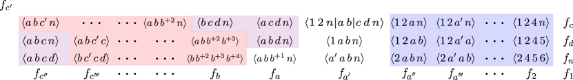
Figure 19. The elements of the extended cluster of $\Sigma_{1}$ of Figure 6 arranged according to the vertices of the rectangle quiver of $\Sigma_{4,n}$, from which they are obtained by applying the mutation sequence of Lemma 9.30.

We note that while Lemma 9.30 was tested extensively via computer checks, it is experimental. The reader who does not want to rely on experimental statements can use the (less-efficient) procedure for going from $\Sigma_{4,n}$ to $\Sigma_{1}$ explained in Remark 9.31.

Remark 9.31.

By [OS17], given any two Plücker seeds $\Sigma$ and $\Sigma^{\prime}$ for $\operatorname{Gr}_{4,n}$, one can find a sequence of mutations at $4$-valent vertices that does not involve mutating at any Plücker coordinate that $\Sigma$ and $\Sigma^{\prime}$ have in common. Thus a (less-efficient) alternative to to Lemma 9.30 is to start at the rectangles seed and randomly mutate at $4$-valent vertices labeled by Plücker coordinates which are not in $\Sigma_{1}$, until one arrives at the seed $\Sigma_{1}$.

Proposition 9.32 (A mutation sequence from $\operatorname{Fr}(\Sigma_{1})$ to $\tilde{\Sigma}_{D}$).

Let $D\in\mathcal{CD}_{n,k}$ be a chord diagram and $D_{L},D_{R}$ its left and right subdiagrams as in Definition 6.10. If $\boldsymbol{\mu}^{(L)}$ and $\boldsymbol{\mu}^{(R)}$ are mutation sequences from $\Sigma_{0}^{L}$ and $\Sigma_{0}^{R}$ (shown in Figure 5) to $\tilde{\Sigma}_{D_{L}}$ and $\tilde{\Sigma}_{D_{R}}$, respectively, then $\boldsymbol{\mu}^{(R)}\boldsymbol{\mu}^{(L)}$ is a mutation sequence from $\operatorname{Fr}(\Sigma_{1})$ to $\tilde{\Sigma}_{D}$.

Proof.

By Theorem 4.7 and Proposition 3.24, the seed $\Sigma_{0}^{L}\sqcup\Sigma_{0}^{R}$ is similar to $\operatorname{Fr}(\Sigma_{1})$, and hence the seed $\boldsymbol{\mu}^{(R)}\boldsymbol{\mu}^{(L)}(\Sigma_{0}^{L}\sqcup\Sigma_{0}^{R})=\tilde{\Sigma}_{D_{L}}\sqcup\tilde{\Sigma}_{D_{R}}$ is similar to $\boldsymbol{\mu}^{(R)}\boldsymbol{\mu}^{(L)}(\operatorname{Fr}(\Sigma_{1}))$, that is, $\Psi(\tilde{\Sigma}_{D_{L}}\sqcup\tilde{\Sigma}_{D_{R}})\propto\boldsymbol{\mu}^{(R)}\boldsymbol{\mu}^{(L)}(\operatorname{Fr}(\Sigma_{1}))$. Therefore when we apply the rescaled product promotion map, we obtain $\overline{\Psi}(\tilde{\Sigma}_{D_{L}}\sqcup\tilde{\Sigma}_{D_{R}})=\boldsymbol{\mu}^{(R)}\boldsymbol{\mu}^{(L)}(\operatorname{Fr}(\Sigma_{1}))$. It follows that $\boldsymbol{\mu}^{(R)}\boldsymbol{\mu}^{(L)}(\operatorname{Fr}(\Sigma_{1}))$ contains the cluster variables $\overline{\Psi}(\widetilde{\mathbf{x}}(D_{L})\cup\widetilde{\mathbf{x}}(D_{R}))$. The seed $\boldsymbol{\mu}^{(R)}\boldsymbol{\mu}^{(L)}(\operatorname{Fr}(\Sigma_{1}))$ also contains the variables $\{\bar{\beta}_{k},\bar{\gamma}_{k},\bar{\delta}_{k},\bar{\varepsilon}_{k}\}\cup\{f_{c},f_{d},f_{a-1}\}$ because these are frozen in $\operatorname{Fr}(\Sigma_{1})$. Therefore $\boldsymbol{\mu}^{(R)}\boldsymbol{\mu}^{(L)}(\operatorname{Fr}(\Sigma_{1}))$ contains the entire cluster $\widetilde{\mathbf{x}}(D)$, defined in Theorem 9.1, and hence coincides with $\tilde{\Sigma}_{D}$. ∎

By combining the previous results, we obtain a recursive construction of the mutation sequence from the rectangles seed $\Sigma_{4,n}$ to $\tilde{\Sigma}_{D}$.

Theorem 9.33 (Recursive algorithm for $\tilde{\Sigma}_{D}$).

Let $\tilde{\Sigma}_{D}$ be the seed associated to a chord diagram $D\in\mathcal{CD}_{n,k}$. As before, let $c=n-2$ and $d=n-1$. The following is an inductive algorithm for constructing the mutation sequence from the rectangles seed $\Sigma_{4,n}$ to $\tilde{\Sigma}_{D}$.

• Suppose that $D$ has no chord ending at $(c,d)$. Let $D^{\prime}$ be the chord diagram on $\{1,2,\dots,c,\widehat{d},n\}$ obtained from $D$ by removing the penultimate marker $d$. By induction we know the mutation sequence from the rectangles seed for $\operatorname{Gr}_{4,\{1,\dots,c,\widehat{d},n\}}$ to $\tilde{\Sigma}_{D^{\prime}}$, so by Lemma 9.29, we can obtain the mutation sequence from the rectangles seed $\Sigma_{4,n}$ to $\tilde{\Sigma}_{D}$.

• Suppose that the rightmost top chord ends at $(c,d)$, that is, $D_{\operatorname{{\it k}}}=(a,b,c,d)$. Let $N_{L}=\{1,2,\dots,a,b,n\}$ and $N_{R}=\{b,\dots,c,d,n\}$, with $D_{L}$ and $D_{R}$ the left and right subdiagrams of $D$. Then Proposition 9.32 gives a mutation sequence from $\operatorname{Fr}(\Sigma_{1})$ to $\tilde{\Sigma}_{D}$, and Lemma 9.30 gives a mutation sequence from the rectangles seed $\Sigma_{4,n}$ to $\Sigma_{1}$, so by concatenating them, we obtain a mutation sequence from $\Sigma_{4,n}$ to $\tilde{\Sigma}_{D}$.

Remark 9.34.

It is possible to generalize Theorem 9.33 to the case of general BCFW tiles. Recall from Definition 6.16 that general BCFW cells are built by a sequence of operations consisting of the BCFW product, inserting a marker, performing a cyclic shift, and performing a reflection. Since we have mutation sequences corresponding to the cyclic shift (cf. Lemma 3.15) and reflection (cf. Proposition 3.17), it is possible to extend Theorem 9.33 to produce a mutation sequence from the rectangles seed to the seed associated to any general BCFW tile.

10. Proofs about the BCFW product

Recall the BCFW map and BCFW product from Definitions 5.2 and 5.4. In this section, we show the effect of the BCFW product at the level of matroids under appropriate hypotheses (cf. 5.7). Under the same hypotheses, we show that the BCFW map is injective, and describe the closure and boundary of $S_{L}\bowtie S_{R}$. We also verify every BCFW cell satisfies these hypotheses.

Lemma 10.1 (Positroids and BCFW product).

Let $S_{L}\subset{\operatorname{Gr}}^{\geq 0}_{k_{L},N_{L}}$ and $S_{R}\subset{\operatorname{Gr}}^{\geq 0}_{k_{R},N_{R}}$ be positroid cells as in 5.7, with associated positroids $\mathcal{P}_{L}$ and $\mathcal{P}_{R}$, and plabic graphs $G_{L}$ and $G_{R}$. Let $\mathcal{P}_{L}^{\prime}$ and $\mathcal{P}_{R}^{\prime}$ be the positroids corresponding to $G^{\prime}_{L}$ and $G^{\prime}_{R}$ (shown at the right of Figure 20); note that $G^{\prime}_{L}$ and $G^{\prime}_{R}$ can be regarded as subgraphs of $G_{L}\bowtie G_{R}$.

Then the bases of the positroid $\mathcal{P}_{L}\bowtie\mathcal{P}_{R}$ of $S_{L}\bowtie S_{R}$ are exactly the sets $I_{L}\sqcup\{f\}\sqcup I_{R}$ where $I_{L},f,I_{R}$ are disjoint and satisfy one of the following:

	$I_{L}$	$f$	$I_{R}$
(1)	$I_{L}\in\mathcal{P}_{L},~{}b\notin I_{L}$	$a$	$I_{R}\in\mathcal{P}_{R}^{\prime}$
(2)	$I_{L}\in\mathcal{P}_{L}$	$b$	$I_{R}\in\mathcal{P}_{R}^{\prime}$
(3)	$I_{L}\in\mathcal{P}_{L}^{\prime}$	$c$	$I_{R}\in\mathcal{P}_{R},~{}d\notin I_{R}$
(4)	$I_{L}\in\mathcal{P}_{L}^{\prime}$	$d$	$I_{R}\in\mathcal{P}_{R}$
(5)	$I_{L}\in\mathcal{P}_{L}^{\prime}$	$n$	$I_{R}\in\mathcal{P}_{R}$
(6)	$I_{L}\in\mathcal{P}_{L}^{\prime}$	$n$	$(I_{R}\setminus\{c\})\cup\{d\}\in\mathcal{P}_{R}$

Proof.

We prove the lemma by analyzing the possible source sets of perfect orientations of $G_{L}\bowtie G_{R}$, which by Proposition A.7 and Theorem A.10, give rise to the bases of $\mathcal{P}_{L}\bowtie\mathcal{P}_{R}$.

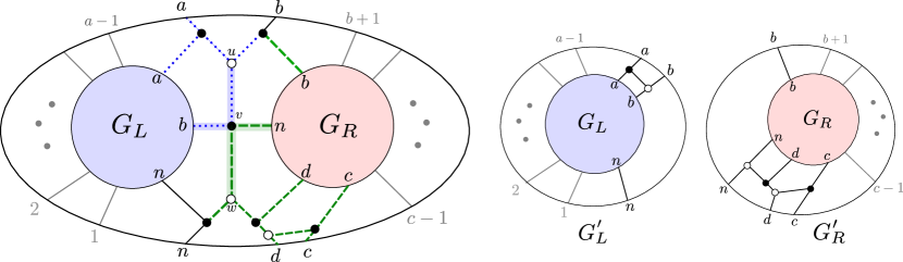
Figure 20. On the left, $G_{L}\bowtie G_{R}$ with edge colorings used in the proof of Lemma 10.1. Center and right, the graphs $G_{L}^{\prime},G_{R}^{\prime}$ mentioned in the statement of the same result.

In any perfect orientation $\mathcal{O}$ of $G_{L}\bowtie G_{R}$, either the dashed green highlighted edges or the dotted blue highlighted edges must form a directed path and the other highlighted edges of Figure 20 must be oriented towards the vertex $v$. If the blue highlighted edges form a directed path, then $\mathcal{O}$ restricted to the blue edges is a perfect orientation of $G_{L}^{\prime}$; similarly with the green edges and $G_{R}^{\prime}$.

Consider a perfect orientation $\mathcal{O}$ of $G_{L}\bowtie G_{R}$.

Case 1: Suppose the green highlighted edges are a directed path in $\mathcal{O}$. Then, depending on the orientation of the edges incident to $u$, we are in one of the cases in Figure 21 where edges $e,e^{\prime}$ form a directed path.

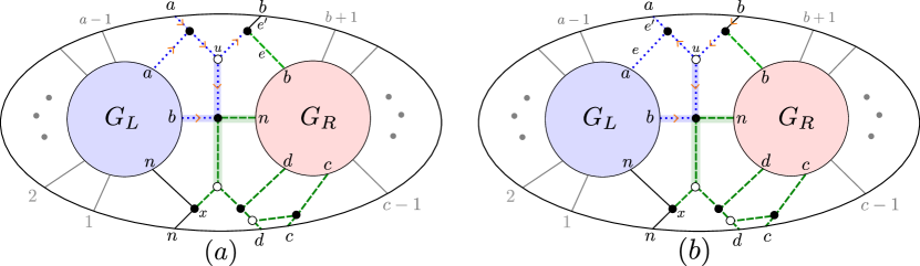
Figure 21.

In (a), the restriction $\mathcal{O}_{L}$ of $\mathcal{O}$ to $G_{L}$ is a perfect orientation where $a,b$ are sinks. The restriction $\mathcal{O}_{R}^{\prime}$ of $\mathcal{O}$ to $G_{R}^{\prime}$ is a perfect orientation whose source set must be disjoint from that of $\mathcal{O}_{L}$ (because only one edge may be oriented away from vertex $x$, $n$ may not be a source in both $\mathcal{O}_{L}$ and $\mathcal{O}_{R}$). Any such perfect orientations of $G_{L},G_{R}^{\prime}$ may arise as $\mathcal{O}_{L},\mathcal{O}_{R}^{\prime}$. The sources of $\mathcal{O}$ are precisely $a$, the sources of $\mathcal{O}_{L}$ and the sources of $\mathcal{O}_{R}^{\prime}$. So this case shows that all sets in (1) are bases of $\mathcal{P}_{L}\bowtie\mathcal{P}_{R}$. Using similiar logic, case (b) shows that all sets in (2) are bases of $\mathcal{P}_{L}\bowtie\mathcal{P}_{R}$.

Case 2: Suppose the blue highlighted edges are a directed path in $\mathcal{O}$. Then, depending on the orientation of the edges incident to $w$, we are in one of the cases in Figure 22.

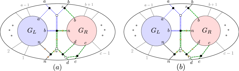
Figure 22.

In (a), the restriction $\mathcal{O}_{L}^{\prime}$ of $\mathcal{O}$ to $G_{L}^{\prime}$ has $n$ as a sink. The restriction $\mathcal{O}_{R}$ of $\mathcal{O}$ to $G_{R}$ also has $n$ as a sink, and has source set disjoint from that of $\mathcal{O}_{L}^{\prime}$, again because only one edge may be oriented away from $x$. These are the only conditions on $\mathcal{O}_{L}^{\prime}$ and $\mathcal{O}_{R}$. Fixing $\mathcal{O}_{L}^{\prime}$ and $\mathcal{O}_{R}$ with sources $I_{L},I_{R}$, one can find $\mathcal{O}$ with sources $I_{L}\cup\{n\}\cup I_{R}$. If $d\in I_{R}$ and $c$ is not, there is another choice of $\mathcal{O}$, with sources $I_{L}\cup\{n\}\cup(I_{R}\setminus\{d\}\cup\{c\})$. This covers cases (5) and (6), and there are no further possibilities for $\mathcal{O}$. In (b), $\mathcal{O}_{R}$ has sinks $d,n$ and $\mathcal{O}_{L}^{\prime},\mathcal{O}_{R}$ have disjoint source sets. The sources of $\mathcal{O}$ are the sources of $\mathcal{O}_{L}^{\prime},\mathcal{O}_{R}$ and either $c$ or $d$. This covers cases (3) and (4).

∎

Proposition 10.2.

Let $S_{L}\subset{\operatorname{Gr}}^{\geq 0}_{k_{L},N_{L}}$ and $S_{R}\subset{\operatorname{Gr}}^{\geq 0}_{k_{R},N_{R}}$ be positroid cells as in 5.7. Then $\iota_{\bowtie}$ is injective on $S_{L}\times\operatorname{Gr}_{1,5}^{\scriptscriptstyle>0}\times S_{R}$.

Proof.

By Proposition 5.8 (1), the image $\iota_{\bowtie}(S_{L}\times\operatorname{Gr}_{1,5}^{>0}\times S_{R})$ is equal to the cell $S_{L}\bowtie S_{R}$. Pick a point $V\in S_{L}\bowtie S_{R}$ and choose any preimage $(A,[\alpha:\beta:\gamma:\delta:\epsilon],B)$. Let $M$ be the representative matrix of $V$ resulting from this choice; that is $M$ is the matrix $(*)$ in Figure 10.

We first express $[\alpha:\beta:\gamma:\delta:\epsilon]$ in terms of Plücker coordinates of $V$. Let $I_{L}$ be a basis for $\mathcal{P}_{L}$ avoiding $\{a,b,n\}$ and let $I_{R}$ be a basis for $\mathcal{P}_{R}$ avoiding $\{b,c,d,n\}$. Because adding bridges does not remove bases (cf. Theorem A.15), Lemma 10.1 implies that $I_{f}:=I_{L}\sqcup\{f\}\sqcup I_{R}$ is a basis of $\mathcal{P}_{L}\bowtie\mathcal{P}_{R}$ for $f\in\{a,b,c,d,n\}$. Now, the submatrix of $M$ on columns $I_{f}$ has a single non-zero entry in the $(k_{L}+1)$th row (which is one of $\alpha,\beta,\pm\gamma,\pm\delta,\pm\epsilon$), which is in column $f$. Deleting row $a$ and column $f$ from the submatrix gives a block-diagonal matrix with determinant $\pm Q\neq 0$. So we have

$$\langle I_{a}\rangle_{M}=\alpha\cdot Q,\qquad\langle I_{b}\rangle_{M}=\beta\cdot Q,\qquad\langle I_{c}\rangle_{M}=\gamma\cdot Q,\qquad\langle I_{d}\rangle_{M}=\delta\cdot Q,\qquad\langle I_{n}\rangle_{M}=\epsilon\cdot Q,$$

or in other words that

(27) $$[\alpha:\beta:\gamma:\delta:\epsilon]=[\langle I_{a}\rangle_{V}:\langle I_{b}\rangle_{V}:\langle I_{c}\rangle_{V}:\langle I_{d}\rangle_{V}:\langle I_{n}\rangle_{V}].$$

Now, we recover $A,B$. Let

$$V_{L}^{\prime}:=V\cap\operatorname{span}(e_{1},\dots,e_{a},e_{b},e_{n})\text{ and }V_{R}^{\prime}:=V\cap\operatorname{span}(e_{b},\dots,e_{c},e_{d},e_{n}).$$

We claim that $V_{L}^{\prime}=A\cdot y_{a}(\frac{\alpha}{\beta})$ and $V_{R}^{\prime}=B\cdot y_{d}(\frac{\delta}{\epsilon})\cdot y_{c}(\frac{\gamma}{\delta})$ (that is, $V_{L}^{\prime}$ and $V_{R}^{\prime}$ are elements of $S_{\mathcal{P}_{L}^{\prime}}$ and $S_{\mathcal{P}_{R}^{\prime}}$, using the notation of Lemma 10.1). The containment $\supset$ is clear in both cases. For the containment $\subset$, it suffices to show $\dim V_{L}^{\prime}=k_{L}$ and $\dim V_{R}^{\prime}=k_{R}$.

Any vector in $V_{L}^{\prime}\cap V_{R}^{\prime}$ would be in $V\cap\operatorname{span}(e_{b},e_{n})$. However, if there existed $v\in V\cap\operatorname{span}(e_{b},e_{n})$, then all nonzero Plücker coordinates of $V$ would contain either $b$ or $n$. The basis $I_{a}$ constructed above contains neither $b$ nor $n$, so such a $v$ cannot exist. Thus $V_{L}^{\prime}\cap V_{R}^{\prime}$ is trivial. Let $w$ denote the span of the $(k_{L}+1)$st row of $M$. Note that $w$ has trivial intersection with $V_{L}^{\prime}$ and with $V_{R}^{\prime}$ since $\alpha,\beta,\gamma,\delta,\epsilon$ are all nonzero. So we have

$$V=w+V_{L}^{\prime}+V_{R}^{\prime}=w\oplus V_{L}^{\prime}\oplus V_{R}^{\prime}$$

and $\dim V_{L}^{\prime}+V_{R}^{\prime}=k-1=k_{L}+k_{R}$. Since $V_{L}^{\prime}$ and $V_{R}^{\prime}$ have dimensions at least $k_{L}$ and $k_{R}$, respectively, we conclude that $\dim V_{L}^{\prime}=k_{L}$ and $\dim V_{R}^{\prime}=k_{R}$ as desired.

Since $V_{L}^{\prime}=A\cdot y_{a}(\frac{\alpha}{\beta})$ and $V_{R}^{\prime}=B\cdot y_{d}(\frac{\delta}{\epsilon})\cdot y_{c}(\frac{\gamma}{\delta})$, we have

(28) $$A=V_{L}^{\prime}\cdot y_{a}\left(-\frac{\alpha}{\beta}\right)\qquad\text{and}\qquad B=V_{R}^{\prime}\cdot y_{c}\left(-\frac{\gamma}{\delta}\right)\cdot y_{d}\left(-\frac{\delta}{\epsilon}\right).$$

Combining (27) and (28), we see that the preimage of $V$ under $\iota_{\bowtie}$ is uniquely determined by $V$; in other words, $\iota_{\bowtie}$ is injective. ∎

Remark 10.3.

The line $w$ in the proof of Proposition 10.2 can also be defined as $w:=V\cap\operatorname{span}(e_{a},e_{b},e_{c},e_{d},e_{n})$. Indeed, the containment $\subset$ is clear. If the right hand side had dimension at least 2, this would imply the existence of a vector in $V_{L}^{\prime}\cap\operatorname{span}(e_{a},e_{b},e_{n})$ or $V_{R}^{\prime}\cap\operatorname{span}(e_{b},e_{c},e_{d},e_{n})$. Then all nonzero Plücker coordinates of $V$ contain either $a,b,$ or $n$ in the first case, or $b,c,d$ or $n$ in the second case. But in the first case, the Plücker coordinate $\langle I_{c}\rangle$ defined in the proof—or in the second case $\langle I_{a}\rangle$ defined in the proof—does not contain any of these indices.

Now we turn to the closure and boundary of $S_{L}\bowtie S_{R}$, which almost have a product structure. This will be used when analyzing the facets of BCFW tiles. We need the following lemma.

Lemma 10.4.

Let $S_{L}\subset{\operatorname{Gr}}^{\geq 0}_{k_{L},N_{L}}$ and $S_{R}\subset{\operatorname{Gr}}^{\geq 0}_{k_{R},N_{R}}$ be positroid cells as in 5.7, then $P:=\iota_{\bowtie}(S_{L}\times\operatorname{Gr}_{1,5}^{\scriptscriptstyle>0}\times S_{R})=S_{L}\bowtie S_{R}$ and each element of $\binom{\{a,b,c,d,n\}}{4}$ is coindependent for $P$.

Proof.

For the first statement, take $J\in\binom{\{a,b,c,d,n\}}{4}$ and write $\{f\}=\{a,b,c,d,n\}\setminus J.$ Choose a basis $I_{R}$ for $S_{R},$ avoiding $b,c,d,n,$ and a basis $I_{L}$ for $S_{L}$ avoiding $a,b,n.$ Then by Lemma 10.1 $I=I_{L}\cup I_{R}\cup\{f\}$ is a basis for $P.$

∎

For a subset $S\subset\operatorname{Gr}_{k,n}^{\scriptscriptstyle\geq 0}$, we use $\overline{S}$ to denote its closure in the Euclidean topology on $\operatorname{Gr}_{k,n}^{\scriptscriptstyle\geq 0}$.

Lemma 10.5 (Boundary of $S_{L}\bowtie S_{R}$).

Let $C_{abcdn}\subset\operatorname{Gr}_{k,n}^{\scriptscriptstyle\geq 0}$ be the union of cells for which some element of $\binom{\{a,b,c,d,n\}}{4}$ is not coindependent. Let $S:=S_{L}\bowtie S_{R}$, with $S_{L},S_{R}$ as in 5.7. Then

(29) $$\overline{S}=(\overline{S}\cap C_{abcdn})\sqcup S\sqcup\bigsqcup_{(S_{L}^{\prime},S_{R}^{\prime})\in\mathcal{C}}S_{L}^{\prime}\bowtie S^{\prime}_{R},$$

where the union is over the collection $\mathcal{C}$ of pairs $(S_{L}^{\prime},S_{R}^{\prime})\neq(S_{L},S_{R})$ such that $S_{L}^{\prime}\subset\overline{S_{L}},S_{R}^{\prime}\subset\overline{S_{R}}$ and $\{a,b,n\}$ and $\{b,c,d,n\}$ are coindependent for $S_{L}^{\prime}$ and $S_{R}^{\prime}$ respectively. Thus,

$$\partial\overline{S}=(\partial\overline{S}\cap C_{abcdn})\sqcup\bigsqcup_{(S_{L}^{\prime},S_{R}^{\prime})\in\mathcal{C}}S_{L}^{\prime}\bowtie S^{\prime}_{R}.$$

Proof.

By Theorem A.12, $\overline{S}$ is the union of $S$ together with any cells we get by deleting one or more of the edges of $G_{L}\bowtie G_{R}$.

Let $G$ be the plabic graph $G_{L}\bowtie G_{R}$. We now show that if we delete some edges of $G_{L}$ (respectively $G_{R}$), obtaining a graph $G^{\prime}_{L}$ (respectively, $G^{\prime}_{R}$) corresponding to a cell $S^{\prime}_{L}$ in which $\{a,b,n\}$ (respectively, $\{b,c,d,n\}$) fails to be coindependent, then the cell $S^{\prime}$ corresponding to the resulting graph $G^{\prime}$ will lie in $C_{abcdn}$. Suppose that $\{a,b,n\}$ fails to be coindependent for $G^{\prime}_{L}$. Then any perfect orientation $\mathcal{O}$ of $G^{\prime}_{L}$ must have a source at $a$, $b$, or $n$. Suppose $\mathcal{O}$ has a source at $a$. Then the edge of $G$ emanating from the vertex of $G_{L}$ labeled $a$ must be directed towards $a$. But now any extension of $\mathcal{O}$ to a perfect orientation of $G^{\prime}$ must have a source at the external vertex labeled $a$. Similarly, if the perfect orientation $\mathcal{O}$ of $G^{\prime}_{L}$ has a source at $b$, then any extension of $\mathcal{O}$ to a perfect orientation of $G^{\prime}$ must have a source at either the external vertex $a$ or $b$ of $G^{\prime}$. Finally, if $\mathcal{O}$ has a source at the vertex $n$ of $G^{\prime}_{L}$, then any extension of $\mathcal{O}$ must have a source at the external vertex $n$ of $G^{\prime}$. This shows that $\{a,b,n\}$ fails to be coindependent for $S^{\prime}$ so $S^{\prime}$ lies in $C_{abcdn}.$ The proof for $G_{R}$ is analogous.

Finally we can check by hand that if we delete any edge of the butterfly, some element of ${\{a,b,c,d,n\}\choose 4}$ will fail to be coindependent, where we use the characterization of Remark 5.6. For example, if we delete the $u-v$ edge in Figure 20, then it is impossible to find a perfect orientation in which $a$ and $b$ are sinks. If we delete the $v-w$ edge, it is impossible to find a perfect orientation in which $c,d,n$ are sinks. The other cases are similar. ∎

Finally, we verify that BCFW cells always fulfill the assumptions of Propositions 5.8, 10.2 and 10.5.

Definition 10.6.

We say that $P\subset\operatorname{Gr}_{k,n}^{\scriptscriptstyle\geq 0}$ is 4-coindependent if every 4-element subset of $[n]$ is co-independent for $P$.

The BCFW product preserves 4-coindependence, which means that taking the BCFW product of two BCFW cells is the same as applying $\iota_{\bowtie}$ to them.

Corollary 10.7.

If $S_{L},S_{R}$ are 4-coindependent, then $S_{L}\bowtie S_{R}$ is as well. Therefore all BCFW cells are 4-coindependent.

Proof.

We first note that 4-coindependence is preserved under cyclic rotation, reflection, and adding a zero column, and all positroid cells for $k=0$ are 4-coindependent. So the second statement follows from the first.

Let $\mathcal{P}_{L},\mathcal{P}_{R},\mathcal{P}_{L}^{\prime},\mathcal{P}_{R}^{\prime}$ be as in Lemma 10.1. Using Proposition A.7, we note that if $J\in\mathcal{P}_{L}$, then $J\in\mathcal{P}_{L}^{\prime}$ as well, and similarly for $\mathcal{P}_{R},\mathcal{P}_{R}^{\prime}$. Thus our assumptions imply $\mathcal{P}_{L}^{\prime}$ and $\mathcal{P}_{R}^{\prime}$ are 4-coindependent.

Let $B\in\binom{[n]}{4}$ be a quadruple of indices. We will show that there exists $I\in\binom{[n]\setminus B}{k}$ which is a basis of $\mathcal{P}_{L}\bowtie\mathcal{P}_{R}$. Let $B_{L}=B\cap N_{L}$ and $B_{R}=B\cap N_{R}$.

1. If $B\subset N_{R}$, then by 4-coindependence for $\mathcal{P}_{R}^{\prime}$, there is a basis $I_{R}$ of $\mathcal{P}_{R}^{\prime}$ avoiding $B$. By assumption, $\mathcal{P}_{L}$ has a basis $I_{L}$ which avoids $a,b,n$ and thus is disjoint from $I_{R}$ and from $B$. Set $I=I_{L}\sqcup\{a\}\sqcup I_{R}$. By Lemma 10.1 (1), $I$ is a basis of $\mathcal{P}_{L}\bowtie\mathcal{P}_{R}$, and it avoids $B$ by construction.

2. If $B\subset N_{L}$, a similar argument as above (now using Lemma 10.1(4)) gives a basis $I=I_{L}\sqcup\{d\}\sqcup I_{R}$ which avoids $B$, where $I_{L}\in\mathcal{P}_{L}^{\prime}$ avoids $B$ and $I_{R}\in\mathcal{P}_{R}$ avoids $b,c,d,n$.

3. Suppose $B$ is not contained in $N_{R}$ or $N_{L}$ and $b\notin B$. This implies that $|B_{L}|+|B_{R}|\leq 5$, so one of $B_{L},B_{R}$ has size at most 2. Add $n$ to the smaller of the two; denote the new sets by $B_{L}^{\prime}$ and $B_{R}^{\prime}$. Let $I_{R}$ be a basis of $\mathcal{P}_{R}^{\prime}$ avoiding $B_{R}^{\prime}\cup\{b\}$ and let $I_{L}$ be a basis of $\mathcal{P}_{L}$ avoiding $B_{L}^{\prime}\cup\{b\}$. Then $I=I_{R}\sqcup\{b\}\sqcup I_{L}$ is a basis by Lemma 10.1 (2) and avoids $B$.

4. Suppose $B$ is not contained in $N_{R}$ or $N_{L}$ and $b\in B$. Then for some $f\in\{c,d,n\}$, we have $f\notin B$. If possible, choose $f=d$ or $f=n$; otherwise, let $f=c$ (that is, only set $f=c$ if $d,n\in B$). Then let $I_{L}$ be a basis of $\mathcal{P}_{L}^{\prime}$ avoiding $B_{L}\cup\{n\}$ and let $I_{R}$ be a basis of $\mathcal{P}_{R}$ avoiding $B_{R}\cup\{f\}$. The sets $I_{L},I_{R}$ are disjoint, since both avoid $b$ and $I_{L}$ avoids $n$. They are both disjoint from $\{f\}$ by construction, and if $f=c$, then $d\notin I_{R}$. So by Lemma 10.1 (3), (4) or (5), $I=I_{R}\sqcup\{f\}\sqcup I_{L}$ is a basis.

∎

11. The proof that BCFW cells give tiles

The main goal of this section is to show how to invert the amplituhedron map on the image of a BCFW cell, thus proving Theorem 7.7, which shows that BCFW cells map injectively into the amplituhedron. In Section 11.1, Section 11.2, and Section 11.3 we will explain how signs of functionaries on tiles evolve when we apply the operations of cyclic shift, reflection, and promotion. In Section 11.4 we will explain a useful way of writing the rows of the BCFW matrix. Finally in Section 11.5 we will prove Theorem 7.7.

11.1. How signs of functionaries evolve

We need the following definitions, which strengthen the notion of the sign of a functionary on a tile (c.f. Definition 2.18).

Definition 11.1.

A rational functionary $F$ has strong sign $+1$ or is strongly positive on the image of $S$ if for all $C\in S$, $F(CZ)$ can be written as a ratio of polynomials in the Plücker coordinates of $C$ and maximal minors of $Z$ with all coefficients of sign $+1$. A rational functionary has strong sign $-1$ or is strongly negative on the image of $S$ if it is the negative of a functionary with strong sign $+1$ on the image of $S$.

Note that if $F$ has strong sign $s$ on the image of $S$, it also has sign $s$ on the image of $S$. The converse may not be true.

Say $S$ is a cell and $S^{\prime}$ is obtained from $S$ by applying an operation from Definition 6.1. The following two theorems (which will be proved in Section 11.2 and Section 11.3) show that if a functionary $F$ has fixed sign on the image of $S$, then there is a related functionary $F^{\prime}$ with a fixed sign on the image of $S^{\prime}$.

Theorem 11.2 (Signs under dihedral group and pre).

Let $S\subset\operatorname{Gr}_{k,n}^{\scriptscriptstyle\geq 0}$ be a positroid cell. Suppose that $F$ is a pure rational functionary with (strong) sign $s$ on $Z_{S}^{\circ}$. Then

$$\begin{cases}F\\ \operatorname{cyc}^{-*}F\\ \operatorname{refl}^{*}F\end{cases}\text{ has (strong) sign }\begin{cases}s\\ (-1)^{k\deg_{n}F}s\\ s\end{cases}\text{ on the image of }\begin{cases}\operatorname{pre}_{I}S\\ {\operatorname{cyc}S}\\ {\operatorname{refl}S}\end{cases}.$$

If $B\subset\{-1,0,1\}^{r}$, we define $\operatorname{cl}(B)\subset\{-1,0,1\}^{r}$ to be minimal set of tuples which contains $B$ and is closed under the operation of changing an entry from $\pm 1$ to $0$. In the following, with a slight abuse of notation, we will often denote the promotion $\Psi(F)$ of a functionary $F$ as $\Psi F$.

Theorem 11.3 (Signs under promotion).

Let $S_{L}\subset\operatorname{Gr}_{k_{L},N_{L}}^{\geq 0},S_{R}\subset\operatorname{Gr}_{k_{R},N_{R}}^{\geq 0}$ be positroid cells as in 5.7. Let $F$ be a pure rational functionary with indices contained in $N_{L}$ (resp. $N_{R}$).

1. If $F$ vanishes on the image of $S_{L}$ (resp. $S_{R}$), then $\Psi_{ac}F$ vanishes on the image of $S_{L}\bowtie S_{R}$.

2. If $F$ has strong sign $s\in\{\pm 1\}$ on the image of $S_{L}$ (resp. $S_{R}$), then $\Psi_{ac}F$ has strong sign $(-1)^{(k_{R}+1)\deg_{n}F}s$ (resp. $s$) on the image of $S_{L}\bowtie S_{R}$.

3. Let $(F_{1},\ldots,F_{r})$ be an $r$-tuple of pure rational functionaries with indices in $N_{L}$ (resp. $N_{R}$). Denote by $A\subseteq\{-1,0,1\}^{r}$ the collection of sign vectors $\operatorname{sgn}(F_{1}(Y,Z),\dots,F_{r}(Y,Z))$, where $Z$ varies over $\operatorname{Mat}_{N_{L},k_{L}+4}^{>0}$ and $Y$ varies over $Z_{S_{L}}^{\circ}$ (resp. $Z\in\operatorname{Mat}_{N_{R},k_{R}+4}^{>0},Y\in Z_{S_{R}}^{\circ}$). Let

   $$A^{\prime}=\{((-1)^{(k_{R}+1)\deg_{n}F_{1}}s_{1},\ldots,(-1)^{(k_{R}+1)\deg_{n}F_{r}}s_{r}):(s_{1},\ldots,s_{r})\in A\}\quad(\mbox{resp. }A^{\prime}=A).$$

   Then for all $Z$ and all $Y\in Z_{S_{L}\bowtie S_{R}}^{\circ}$, $\operatorname{sgn}(\Psi_{ac}F_{1},\ldots,\Psi_{ac}F_{r})\in\operatorname{cl}(A^{\prime}).$

Lemma 11.4.

Let $S_{L}\bowtie S_{R}\subset\operatorname{Gr}_{k,n}^{\scriptscriptstyle\geq 0}$, with $S_{L},S_{R}$ as in 5.7. Then the twistor coordinates

$$(-1)^{k_{R}}\langle\!\langle bcdn\rangle\!\rangle,\quad(-1)^{k_{R}+1}\langle\!\langle acdn\rangle\!\rangle,\quad\langle\!\langle abdn\rangle\!\rangle,\quad-\langle\!\langle abcn\rangle\!\rangle,\quad\langle\!\langle abcd\rangle\!\rangle$$

have strong sign $+1$ on the image of $S_{L}\bowtie S_{R}$.

Proof.

Expand each twistor $\langle\!\langle ijlh\rangle\!\rangle$ as in (4). We obtain a sum of products of Plücker coordinate of the matrix $C\in S_{L}\bowtie S_{R}$, and the matrix $Z$. The sum is over all Plücker coordinates of $C$ which are non zero and intersect the set $\{a,b,c,d,n\}$ precisely in the singleton $\{a,b,c,d,n\}\setminus\{i,j,l,h\}.$ It is straightforward to see that all these terms come with the sign in the lemma using Lemma 10.1. Lemma 10.4 shows that the summation is non-empty. ∎

Lemma 11.5.

Let $S$ be a BCFW cell of $\operatorname{Gr}_{k,n}^{\scriptscriptstyle\geq 0}$. For $i,j\in[n-1]$ with $i+1<j$, the twistor $\langle\!\langle i,i+1,j,j+1\rangle\!\rangle$ is strongly positive on $Z_{S}^{\circ}$. For $i\in\{2,\dots,n\}$, the twistor $\langle\!\langle i,i+1,n,1\rangle\!\rangle$ has strong sign $(-1)^{k-1}$ on $Z_{S}^{\circ}$.

Proof.

The proof is almost identical to the proof of the previous lemma. Again we expand the twistor coordinates using (4), and observe that all possible nonzero terms terms come with the sign indicated in the lemma statement. As long as there is at least one Plücker coordinate of $C$ which does not use the indices $i,i+1,j,j+1$ and is nonzero, the summation is non zero. But such a coordinate exists, as $S$ is $4$-coindependent, by Corollary 10.7. ∎

11.2. The proof of Theorem 11.2

In this section and the next, if $F$ is a functionary, we will sometimes write $F(Y,Z)$ where $Y\in\operatorname{Gr}_{k,k+4}$ and $Z\in\operatorname{Mat}_{n,k+4}^{>0}$. We also sometimes write $\langle\!\langle YZ_{I}\rangle\!\rangle$ for the twistor coordinate $\langle\!\langle I\rangle\!\rangle$. Recall that in $\langle\!\langle I\rangle\!\rangle=\langle\!\langle YZ_{I}\rangle\!\rangle$, the elements of $I$ are listed in increasing order.

The following lemma relates twistor coordinates before and after applying $\operatorname{pre}_{i},\operatorname{cyc},\operatorname{refl}$.

Lemma 11.6.

Let $N$ denote the index set of $S$, and let $S^{\prime}$ denote one of $\operatorname{pre}_{i}S,\operatorname{cyc}S,\operatorname{refl}S$. Choose $C^{\prime}\in S^{\prime}$, and $Z^{\prime}$ a positive matrix of the appropriate size. Then there exists $C\in S$ and $Z$ positive so that for all $I\in\binom{N}{4}$,

$$\langle\!\langle CZ~{}Z_{I}\rangle\!\rangle=\begin{cases}\langle\!\langle C^{\prime}Z^{\prime}~{}Z^{\prime}_{I}\rangle\!\rangle&\text{ if }S^{\prime}=\operatorname{pre}_{i}S\\ (-1)^{k\cdot|I\cap\{n\}|}\operatorname{cyc}^{-*}\langle\!\langle C^{\prime}Z^{\prime}~{}Z^{\prime}_{I}\rangle\!\rangle&\text{ if }S^{\prime}=\operatorname{cyc}S\\ \operatorname{refl}^{*}\langle\!\langle C^{\prime}Z^{\prime}~{}Z^{\prime}_{I}\rangle\!\rangle&\text{ if }S^{\prime}=\operatorname{refl}S.\\ \end{cases}$$

Proof.

If $S^{\prime}=\operatorname{pre}_{i}S$, then $Z^{\prime}\in\operatorname{Mat}_{N\cup\{i\},k+4}^{>0}$. The matrices $C$ and $Z$ are respectively defined by deleting the $i$th column of $C^{\prime}$ and the $i$th row of $Z^{\prime}$. It is clear that $CZ=C^{\prime}Z^{\prime}$ and for all $x\in N$, $Z_{x}=Z_{x}^{\prime}$. The equality of twistor coordinates follows.

For the remaining cases, we assume $N=[n]$ to simplify notation. If $S^{\prime}=\operatorname{cyc}S$, then we define $C\in S$ to be the unique element such that $\operatorname{cyc}C=C^{\prime}$. Recall from the definition of cyclic shift (cf. Definition 2.3) that $\operatorname{cyc}C=C\cdot[\operatorname{cyc}_{k,n}]$ where $[\operatorname{cyc}_{k,n}]$ is an $n\times n$ matrix. We define $Z:=[\operatorname{cyc}_{k,n}]Z^{\prime}$, so that $C^{\prime}Z^{\prime}=C[\operatorname{cyc}_{k,n}]Z=CZ$. Note that $Z$ is again a matrix with positive maximal minors.

So we have $\langle\!\langle CZ~{}Z_{I}\rangle\!\rangle=\langle\!\langle C^{\prime}Z^{\prime}~{}Z_{I}\rangle\!\rangle$. We now rewrite the right hand twistor entirely in terms of $Z^{\prime}$. From the definition of $[\operatorname{cyc}_{k,n}]$, we have that $Z_{i}=Z^{\prime}_{i+1}$ for $i<n$ and $Z_{n}=(-1)^{k-1}Z^{\prime}_{1}$. If $I=\{u<v<x<y\}$ does not contain $n$, then

$$\langle\!\langle C^{\prime}Z^{\prime}~{}Z_{I}\rangle\!\rangle=\langle\!\langle C^{\prime}Z^{\prime}~{}Z^{\prime}_{u+1}Z^{\prime}_{v+1}Z^{\prime}_{x+1}Z^{\prime}_{y+1}\rangle\!\rangle=\operatorname{cyc}^{-*}\langle\!\langle C^{\prime}Z^{\prime}~{}Z^{\prime}_{I}\rangle\!\rangle$$

where the last equality holds because the indices are in increasing order. If $I=\{u<v<x<n\}$, then

$$\langle\!\langle C^{\prime}Z^{\prime}~{}Z_{I}\rangle\!\rangle=(-1)^{k-1}\langle\!\langle C^{\prime}Z^{\prime}~{}Z^{\prime}_{u+1}Z^{\prime}_{v+1}Z^{\prime}_{x+1}Z^{\prime}_{1}\rangle\!\rangle=(-1)^{k}\langle\!\langle C^{\prime}Z^{\prime}~{}Z^{\prime}_{1}Z^{\prime}_{u+1}Z^{\prime}_{v+1}Z^{\prime}_{x+1}\rangle\!\rangle$$

and the final twistor is $(-1)^{k}\operatorname{cyc}^{-*}\langle\!\langle C^{\prime}Z^{\prime}~{}Z^{\prime}_{I}\rangle\!\rangle$.

If $S^{\prime}=\operatorname{refl}S$, the proof is quite similar. Recall that $\operatorname{refl}$ is an involution. Define $C:=\operatorname{refl}C^{\prime}$, so that $C^{\prime}=\operatorname{refl}C=P_{k,1,\binom{k}{2}}C[\operatorname{refl}_{n}]$ (cf. Definition 2.3 for the definitions of $P_{k,i,s}$ and $[\operatorname{refl}_{n}]$). We choose $Z=[\operatorname{refl}_{n}]Z^{\prime}P_{k+4,1,\binom{k+4}{2}}$, which again has positive maximal minors. With these choices, $C^{\prime}Z^{\prime}$ is equal to $CZ$ with the first row multiplied by $(-1)^{\binom{k}{2}}$ and the first column multiplied by $(-1)^{\binom{k+4}{2}}$. Note that $Z_{i}$ is $Z^{\prime}_{n-i+1}$ with first entry multiplied by $(-1)^{\binom{k+4}{2}}$. This implies that for $I=\{u<v<x<y\}$,

$$\langle\!\langle CZZ_{u}Z_{v}Z_{x}Z_{y}\rangle\!\rangle=\langle\!\langle C^{\prime}Z^{\prime}Z^{\prime}_{n+1-u}Z^{\prime}_{n+1-v}Z^{\prime}_{n+1-x}Z^{\prime}_{n+1-y}\rangle\!\rangle=\langle\!\langle C^{\prime}Z^{\prime}Z^{\prime}_{n+1-y}Z^{\prime}_{n+1-x}Z^{\prime}_{n+1-v}Z^{\prime}_{n+1-u}\rangle\!\rangle$$

where the first equality uses the fact that the parity of $\binom{k}{2}$ depends only on $k\mod 4$. Since the indices of the rightmost twistor are in increasing order, it is equal to $\operatorname{refl}^{*}\langle\!\langle C^{\prime}Z^{\prime}Z^{\prime}_{I}\rangle\!\rangle$, as desired. ∎

Proof of Theorem 11.2.

We first consider the case when $F$ has sign $s\in\{0,+1,-1\}$ on the image of $S$. We will give the argument for the sign of $\operatorname{cyc}^{-*}F$ on the image of $\operatorname{cyc}S$; the others are very similar. Note that by definition, $\operatorname{cyc}^{-*}F$ has an expression in terms of the cyclic shifts of twistor coordinates $\operatorname{cyc}^{-*}\langle\!\langle I\rangle\!\rangle$. Pick $C^{\prime}\in\operatorname{cyc}S$ and $Z^{\prime}$ positive, and let $C\in S$ and $Z$ be the matrices from Lemma 11.6. Applying Lemma 11.6 separately to each twistor coordinate in $F$, each term gets a sign of $(-1)^{k\deg_{n}F}$ so we see that $F(CZ,Z)=(-1)^{k\deg_{n}F}\operatorname{cyc}^{*}F(C^{\prime}Z^{\prime},Z^{\prime})$. By assumption, $F(CZ,Z)$ has sign $s$, and so $\operatorname{cyc}^{*}F(C^{\prime}Z^{\prime},Z^{\prime})$ has sign $s$ as well. Since $C^{\prime}$ and $Z^{\prime}$ were chosen arbitrarily, this shows $\operatorname{cyc}^{*}F$ has sign $s$ on the image of $\operatorname{cyc}S$.

We now consider the case when $F$ has strong sign $s\in\{+1,-1\}$ on the image of $S$. That is, as a function from $S\times\operatorname{Mat}_{n,k+4}^{>0}$, $F=f(C,Z)/g(C,Z)$ where $f,g$ are polynomials in the Plücker coordinates of $C$ and the maximal minors of $Z$, all coefficients of $f$ are sign $s$ and all coefficients of $g$ are positive. We again will only give the argument for the strong sign of $\operatorname{cyc}^{-*}F$ on the image of $\operatorname{cyc}S$; the others are very similar. Lemma 11.6 implies that for any $C^{\prime}\in\operatorname{cyc}S$ and $Z^{\prime}$ positive, $(-1)^{k\deg_{n}F}\operatorname{cyc}^{-*}F(C^{\prime}Z^{\prime},Z^{\prime})$ is equal to $F(CZ,Z)$, where $C,Z$ are as constructed in the lemma. Thus we have

$$(-1)^{k\deg_{n}F}\operatorname{cyc}^{-*}F(C^{\prime}Z^{\prime},Z^{\prime})=f(C,Z)/g(C,Z).$$

What remains is to rewrite $f(C,Z)$ and $g(C,Z)$ in terms of the Plücker coordinates and maximal minors of $C^{\prime},Z^{\prime}$ without changing the signs of any coefficients. This is straightforward: since $C^{\prime}=\operatorname{cyc}C$, $\langle I\rangle_{C}=\langle I+1\rangle_{C^{\prime}}$, and, similarly, since $Z=\operatorname{cyc}Z^{\prime}$, $\langle I\rangle_{Z}=\langle I-1\rangle_{Z^{\prime}}$. ∎

11.3. The proof of Theorem 11.3

We will treat the case when the indices of $F$ are contained in $N_{R}$. The proof for the other case is similar; we remark on the differences at the end of this section.

Notation 11.7.

For a positroid $S_{R}$ in $\operatorname{Gr}^{\geq 0}_{k_{R},N_{R}}$, we set $S_{R}^{\triangleleft}=\operatorname{Gr}^{>0}_{k_{L},N_{L}}\bowtie S_{R}$, and for a positroid $S_{L}$ of $\operatorname{Gr}^{\geq 0}_{k_{L},N_{L}}$, we set $S_{L}^{\triangleright}=S_{L}\bowtie\operatorname{Gr}^{>0}_{k_{R},N_{R}}.$

Using 11.7, Lemma 10.1 implies that $S_{L}\bowtie S_{R}\subset\overline{S_{R}^{\triangleleft}}$. Indeed, let $\mathcal{P}_{L},\mathcal{P}_{L}^{\prime}$ be as in Lemma 10.1. Every element of $\mathcal{P}_{L},\mathcal{P}_{L}^{\prime}$ is a basis for $\operatorname{Gr}^{>0}_{k_{L},N_{L}}$, so by Lemma 10.1, every basis for $S_{L}\bowtie S_{R}$ is a basis of $S_{R}^{\triangleleft}$.

The proof will utilize the following lemmas.

Lemma 11.8.

$S_{R}^{\triangleleft}$ can be constructed in the following way. Start with $S_{R}.$

• Apply the upper BCFW map to $S_{R}.$

• Perform $\operatorname{inc}_{1},\ldots,\operatorname{inc}_{k_{L}},$ and then $\operatorname{pre}_{k_{L}+1},\ldots,\operatorname{pre}_{a-1}.$

• Apply $y_{n}(t_{1}),y_{1}(t_{2}),\dots y_{k_{L}-1}(t_{k_{L}-1})$ in that order.

• For each $h=1,\ldots,b-k_{L},$ apply the operations $x_{k_{L}+h-1}(t_{k_{L};h}),x_{k_{L}+h-2}(t_{k_{L}-1;h}),\dots,x_{h}(t_{1;h})$ in that order.

The proof is completely analogous to the proof of [ELT21, Lemma 9.6], which goes by comparing the collections of non zero Plücker coordinates for the two descriptions. See Figure 23 for a plabic graph proof of the lemma.

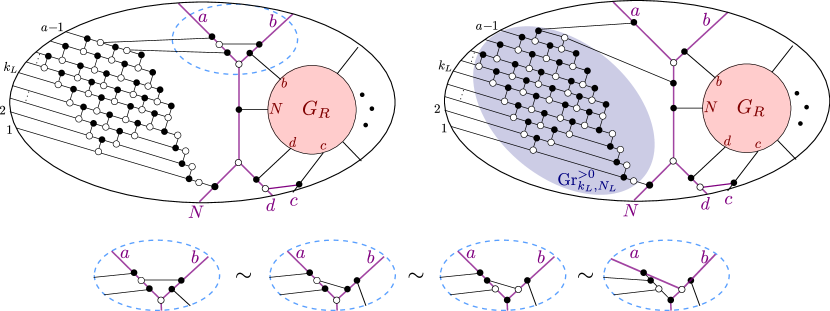
Figure 23. On the upper left, the plabic graph constructed by the sequence of operations in Lemma 11.8. Performing the moves in the bottom row produces the graph on the upper right, which is of the form $G\bowtie G_{R}$ where $G$ a plabic graph for $\operatorname{Gr}_{k_{L},N_{L}}^{>0}$. The graph on the left is thus a plabic graph for $S_{R}^{\triangleleft}$.

Lemma 11.9.

Let $C\in S_{R}^{\triangleleft}$ and $Z\in\operatorname{Mat}_{n,k+4}^{>0}$. Then there exists $C^{\prime}\in S_{R}$ and $Z^{\prime}\in\operatorname{Mat}_{N_{R},k_{R}+4}^{>0}$ such that for any functionary $F$ with indices in $N_{R}$, $\Psi_{ac}F(CZ,Z)=F(C^{\prime}Z^{\prime},Z^{\prime}).$

This follows from [ELT21, Section 4]. For the reader’s convenience, we outline a proof.

Proof.

We will show the lemma holds for each intermediate cell obtained in the process in Lemma 11.8. The first step in Lemma 11.8 is the upper BCFW map. Let $T:=\iota_{\bowtie}(\operatorname{Gr}_{1,5}^{\scriptscriptstyle>0}\times S_{R})$, choose $C\in T$ and choose a positive matrix $Z$. The proof of [ELT21, Lemma 4.28] together with [ELT21, Lemma 4.22] define an element $C^{\prime}\in S_{R}$ and positive matrix $Z^{\prime}$ with the following property: for any functionary $F$ with indices in $N_{R}$, there is a functionary $G$ such that $F(C^{\prime}Z^{\prime},Z^{\prime})=G(CZ,Z)$. [ELT21, Lemma 4.35] implies that $G=\Psi_{ac}F$; this is spelled out more explicitly in [ELT21, Example 4.40]. Note that by Lemma 11.4, the twistor coordinates in [ELT21, Lemma 4.35] are all nonzero on the image of $\iota_{\bowtie}(\operatorname{Gr}_{1,5}^{\scriptscriptstyle>0}\times S_{R})$, so one may divide in [ELT21, Lemma 4.35] to obtain precisely the formulas defining promotion.

Now, let $T$ denote a cell obtained partway through the process described in Lemma 11.8, and $T^{\prime}$ the cell obtained in the previous step. Fix $C\in T$ and $Z$ a positive matrix of the appropriate dimensions. [ELT21, Lemmas 4.18, 4.21 and 4.24] construct $C^{\prime}\in T^{\prime}$ and $Z^{\prime}$ a positive matrix of the appropriate dimensions with the following property:

$(**):$ if $I\in\binom{N_{R}}{4}$ or $I=\{a,b,x,y\}$ where $x,y\in N_{R}$, then the twistor coordinates $\langle\!\langle C^{\prime}Z^{\prime}~{}Z^{\prime}_{I}\rangle\!\rangle$ and $\langle\!\langle CZ~{}Z_{I}\rangle\!\rangle$ are equal.

Consider any functionary $F$ with indices contained in $N_{R}$. All twistor coordinates in $\Psi_{ac}F$ are of the sort appearing in $(**)$, so we have that $\Psi_{ac}F(C^{\prime}Z^{\prime},Z^{\prime})=\Psi_{ac}F(CZ,Z)$. Taking $T=S_{R}^{\triangleleft}$ and iterating, we obtain the lemma statement. ∎

The final lemma involves functionaries with strong sign on the image of a cell, and tracks how the strong sign evolves under various operations.

Lemma 11.10.

We adopt the notation and assumptions of Theorem 11.3 and suppose $F$ has indices contained in $N_{L}$ (resp. $N_{R}$).

1. Suppose $F$ has strong sign $s$ on the image of $S_{L}$ (resp. $S_{R}$). Then for $i\notin N_{L}$ (resp. $i\notin N_{R}$), $F$ has strong sign $s$ on the image of $\operatorname{pre}_{i}(S_{L})$ (resp. $\operatorname{pre}_{i}(S_{R})$). Additionally, $F$ has strong sign $(-1)^{\deg_{n}F}s$ (resp. $s$) on the image of $\operatorname{inc}_{i}(S_{L})$ (resp. $\operatorname{inc}_{i}(S_{R})$).

2. Suppose $F$ has strong sign $s$ on the image of $S_{L}$ (resp. $S_{R}$). Choose $i\notin N_{L}$ (resp. $i\notin N_{R}$). Then $F$ has strong sign $s$ on the image of $x_{i}(\mathbb{R}_{+}).S_{L}$ and $y_{i-1}(\mathbb{R}_{+}).S_{L}$ (resp. $x_{i}(\mathbb{R}_{+}).S_{R}$ and $y_{i-1}(\mathbb{R}_{+}).S_{R}$).

3. If $F$ has strong sign $s$ on the image of $S_{L}$, then $\Psi_{ac}F$ has strong sign $(-1)^{\deg_{n}F}s$ on the image of $\iota_{\bowtie}(S_{L}\times\operatorname{Gr}_{1,5}^{\scriptscriptstyle>0}\times\operatorname{Gr}_{0,\{b,c,d,n\}}^{>0})$. If $F$ has strong sign $s$ on the image of $S_{R}$, then $\Psi_{ac}F$ has strong sign $s$ on the image of $\iota_{\bowtie}(\operatorname{Gr}_{1,5}^{\scriptscriptstyle>0}\times S_{R})$.

Again, the proof of this lemma relies on various results from [ELT21, Section 4].

Proof.

Throughout, we will show the results only for $S:=S_{R}$, except in a few places where there is a difference between the arguments. So we assume that on the image of $S_{R}$, $F=f(C,Z)/g(C,Z)$ where $f,g$ are polynomials in the Plücker coordinates of $C,Z$, the coefficients of $f$ are all of sign $s$ and the coefficients of $g$ are all positive. We will sometimes write $F(Y,Z)$ to make the dependence of $F$ on $Z$ clear. We also write $\langle\!\langle Y~{}Z_{I}\rangle\!\rangle$ instead of $\langle\!\langle uvxy\rangle\!\rangle$.

Proof of (1): The case of $\operatorname{pre}_{i}S$ is shown in Theorem 11.2.

The argument for $\operatorname{inc}_{i}S$ uses [ELT21, Lemma 4.21], which shows that for any $Z^{\prime}$ and $C^{\prime}:=\operatorname{inc}_{i}(C)$, there is a $Z$ such that for each twistor $\langle\!\langle I\rangle\!\rangle$ appearing in $F$, $\langle\!\langle C^{\prime}Z^{\prime}~{}Z^{\prime}_{I}\rangle\!\rangle=\langle\!\langle CZ~{}Z_{I}\rangle\!\rangle$. (There is no sign because $[\ell]\cap I$ is empty, since $I\subset N_{R}$.) We have $\langle I\rangle_{C}=\langle I\cup\{i\}\rangle_{C^{\prime}}$ and by the proof of [ELT21, Lemma 4.21], the same statement holds for $Z,Z^{\prime}$. So adding $i$ to each Plücker coordinate and minor appearing in $f$ and $g$ gives a formula for $F$ on the image of $\operatorname{inc}_{i}(S)$.

The argument for $\operatorname{inc}_{i}(S_{L})$ (assuming $F$ has strong sign $s$ on $S_{L}$) is exactly the same, except that if $n\in I$, then $\langle\!\langle C^{\prime}Z^{\prime}~{}Z^{\prime}_{I}\rangle\!\rangle=-\langle\!\langle CZ~{}Z_{I}\rangle\!\rangle$. So $F(C^{\prime}Z^{\prime},Z^{\prime})=(-1)^{\deg_{n}F}F(CZ,Z)$, and the strong sign of $F$ on the image of $\operatorname{inc}_{\ell}(S_{L})$ is $(-1)^{\deg_{n}F}s$.

Proof of (2): The arguments for $x_{i}$ and $y_{i-1}$ are very similar, so we will only give the $x_{i}$ argument here. Let $S^{\prime}=x_{i}(\mathbb{R}_{+}).S_{R}$.

First, if $S=S^{\prime}$, then the statement is clearly true. So we will assume $S\neq S^{\prime}$, and thus $S\subset\overline{S^{\prime}}$.

Every $C^{\prime}\in S^{\prime}$ can be written uniquely as $Cx_{i}(t)$ for $t>0,~{}C\in S$. The parameter $t$ is the ratio $\langle I\cup\{i+1\}\rangle_{C^{\prime}}/\langle I\cup\{i\}\rangle_{C^{\prime}}$ where $I\subset[n]\setminus\{i,i+1\}$ is any subset such that $I\cup\{i\}$ is a basis of $S$ but $I\cup\{i+1\}$ is not. Such $I$ exists since the matroid of $S^{\prime}$ strictly contains that of $S.$

Fix $Z^{\prime}$. Let $Z=x_{i}(t)Z^{\prime}$, so that $CZ=Cx_{i}(t)Z^{\prime}=C^{\prime}Z^{\prime}$. By [ELT21, Lemma 4.24], $\langle\!\langle C^{\prime}Z^{\prime}~{}Z_{I}^{\prime}\rangle\!\rangle=\langle\!\langle CZ~{}Z_{I}\rangle\!\rangle$ for all twistors appearing in $F$, because $i\notin I$. This implies that $F(C^{\prime}Z^{\prime},Z^{\prime})=F(CZ,Z)=f(C,Z)/g(C,Z)$. What remains is to re-express the right hand side in terms of Plückers of $C^{\prime}$ and $Z^{\prime}$, without changing the signs of any coefficients.

It follows from the proof of [Lam15, Lemma 7.11] that the Plücker coordinates of $C$ are Laurent polynomials in the Plücker coordinates of $C^{\prime}$ with positive coefficients. Maximal minors of $Z$ are positive polynomials in the maximal minors of $Z^{\prime}$ and in $t$, which is the ratio of two Plücker coordinates of $C^{\prime}$. Thus we may rewrite $f(C,Z)/g(C,Z)$ in terms of maximal minors of $Z^{\prime}$ and Plücker coordinates of $C^{\prime}$ without changing the sign of any coefficient.

Proof of (3): Note that $\iota_{\bowtie}(\operatorname{Gr}_{1,5}^{\scriptscriptstyle>0}\times S)=\iota_{\bowtie}(\operatorname{Gr}_{0,\{a,b,n\}}^{>0}\times\operatorname{Gr}_{1,5}^{\scriptscriptstyle>0}\times S)$ can also be described as

$$S_{3}=y_{c}(\mathbb{R}_{+}).y_{d}(\mathbb{R}_{+}).y_{n}(\mathbb{R}_{+}).x_{a}(\mathbb{R}_{+}).\operatorname{inc}_{a}(S).$$

Write

$$S_{1}=y_{n}(\mathbb{R}_{+}).x_{a}(\mathbb{R}_{+}).\operatorname{inc}_{a}(S),~{}~{}S_{2}=y_{d}(\mathbb{R}_{+}).S_{1},~{}~{}S_{3}=y_{c}(\mathbb{R}_{+}).S_{2}.$$

Note that $F$ has strong sign $s$ on the image of $S_{1}$ by (1) and (2).

For $C\in S_{3}$, $C=y_{c}(t).C^{\prime}$ for unique $t>0$ and $C^{\prime}\in S_{2}$. Similarly, $C^{\prime}=y_{d}(s).C^{\prime\prime}$ for unique $s>0$ and $C^{\prime\prime}\in S_{1}.$ Note that $t,s$ can be computed as $\langle I\cup\{c\}\rangle_{C}/\langle I\cup\{d\}\rangle_{C}$, and $\langle I\cup\{d\}\rangle_{C}/\langle I\cup\{n\}\rangle_{C}$ respectively for any $I\in\binom{b+1,\ldots,c-1}{k_{L}}$ such that $I$ is a basis for $S$. Such an $I$ is guaranteed to exist because $\{b,c,d,n\}$ is coindependent for $S$.

Fix $Z$. Let $Z^{\prime}:=y_{c}(t)Z$ and $Z^{\prime\prime}:=y_{d}(s)Z^{\prime}$, so that $C^{\prime\prime}Z^{\prime\prime}=CZ$. Note that $\langle\!\langle C^{\prime\prime}Z^{\prime\prime}~{}Z_{I}^{\prime\prime}\rangle\!\rangle=\langle\!\langle CZ~{}Z_{I}^{\prime\prime}\rangle\!\rangle=\Psi_{ac}\langle\!\langle CZ~{}Z_{I}\rangle\!\rangle$. This implies that $\Psi_{ac}F(CZ,Z)=F(C^{\prime\prime}Z^{\prime\prime},Z^{\prime\prime})$. Since $F$ has strong sign $s$ on the image of $S_{1}$, the right hand side is equal to $p(C^{\prime\prime},Z^{\prime\prime})/q(C^{\prime\prime},Z^{\prime\prime})$ where $p,q$ are polynomials in the Plückers of $C^{\prime\prime},Z^{\prime\prime}$, all coefficients of $p$ have sign $s$ and all coefficients of $q$ are positive. Again, what remains is to re-express this in terms of the Plückers of $C,Z$ without changing the signs of coefficients. Again, the proof of [Lam15, Lemma 7.11] shows that the Plücker coordinates of $C^{\prime\prime}$ are positive Laurent polynomials in the Plücker coordinates of $C^{\prime}$, which are themselves positive Laurent polynomials in the Plücker coordinates of $C$. Since additionally $s,t$ are positive ratios of Plücker coordinates of $C$, we are done.

The argument for the strong sign of $\Psi_{ac}F$ on the image of

$$\iota_{\bowtie}(S_{L}\times\operatorname{Gr}_{1,5}^{\scriptscriptstyle>0}\times\operatorname{Gr}_{0,\{b,c,d,n\}}^{>0})=y_{a}(\mathbb{R}_{+}).y_{b}(\mathbb{R}_{+}).y_{c}(\mathbb{R}_{+}).x_{d}(\mathbb{R}_{+})\circ\operatorname{inc}_{d}\circ\operatorname{pre}_{c}(S_{L})$$

is very similar. The only difference is that (1), (2) imply $F$ has strong sign $(-1)^{\deg_{n}F}s$ on the image of $S_{1}:=y_{b}(\mathbb{R}_{+}).y_{c}(\mathbb{R}_{+}).x_{d}(\mathbb{R}_{+})\circ\operatorname{inc}_{d}\circ\operatorname{pre}_{c}(S_{L}).$ Then essentially the same argument as above shows that $\Psi_{ac}F$ also has strong sign $(-1)^{\deg_{n}F}s$ on the image of $y_{a}(\mathbb{R}_{+}).S_{1}=\iota_{\bowtie}(S_{L}\times\operatorname{Gr}_{1,5}^{\scriptscriptstyle>0}\times\operatorname{Gr}_{0,\{b,c,d,n\}}^{>0}).$

∎

With these lemmas in hand, we proceed to the proof of Theorem 11.3.

Proof of Theorem 11.3.

We assume that the indices in $F$ are contained in $N_{R}$, as the other case is similar. At the end of the proof we will discuss the differences in the other case.

Item (1): Suppose $F$ vanishes on the image of $S_{R}$. By Lemma 11.9, $\Psi_{ac}F$ evaluated on a point of $S_{R}^{\triangleleft}$ is equal to $F$ evaluated on a point of $S_{R}$ (using a different matrix $Z$). Thus, $\Psi_{ac}F$ vanishes on the image of $S_{R}^{\triangleleft}$, and also on the image of $\overline{S_{R}^{\triangleleft}}$. Since $S_{L}\bowtie S_{R}\subset\overline{S_{R}^{\triangleleft}}$, $\Psi_{ac}F$ vanishes on $S_{L}\bowtie S_{R}$, as desired.

Item (2): Suppose $F$ has strong sign $s$ on the image of $S_{R}$. Since $\{a,b,n\}$ is co-independent for $S_{L}$, we may find $1\leq i_{1}<i_{2}<\ldots i_{k_{L}}<a$ such that $B=\{i_{1},i_{2},\dots,i_{k_{L}}\}$ is a basis for $S_{L}$. Let $S^{\prime}\subset\operatorname{Gr}_{k_{L},N_{L}}^{\geq 0}$ be the positroid cell whose only basis is $B$. Define

(30) $$S_{\triangleleft}:=S^{\prime}\bowtie S_{R}=\operatorname{pre}_{N_{L}\setminus(I\cup\{a,b,n\})}\circ\operatorname{inc}_{i_{k_{L}}}\circ\cdots\circ\operatorname{inc}_{i_{2}}\circ\operatorname{inc}_{i_{1}}(\iota_{\bowtie}(\operatorname{Gr}_{1,5}^{\scriptscriptstyle>0}\times S_{R})).$$

Since the bases of $S^{\prime}$ are a subset of the bases in $S_{L}$, it is easy to see using Lemma 10.1 that every basis of $S_{\triangleleft}$ is a basis of ${S_{L}\bowtie S_{R}}$. So we have

(31) $$S_{\triangleleft}\subseteq\overline{S_{L}\bowtie S_{R}}\subseteq\overline{S_{R}^{\triangleleft}}.$$

Using Lemma 11.10 on $N_{R},S_{R}$, we will show that $\Psi_{ac}F$ has strong sign $s$ on the images of both $S_{R}^{\triangleleft}$ and $S_{\triangleleft}.$

We deal with the sign of $\Psi_{ac}F$ on the image of $S_{R}^{\triangleleft}$ first. In Lemma 11.8, we apply the upper BCFW map, $\operatorname{inc}_{\ell},\operatorname{pre}_{\ell}$ for $\ell\notin N_{R}$, and $x_{i},y_{i-1}$ for $i\notin N_{R}$. So by Lemma 11.10, $\Psi_{ac}F$ has strong sign $s$ on the image of $S_{R}^{\triangleleft}$.

Since the operations applied in (30) are a subset of those applied in Lemma 11.8, an identical argument shows that $\Psi_{ac}F$ has strong sign $s$ on the image of $S_{\triangleleft}$.

By (31), $\Psi_{ac}F$ having strong sign $s$ on the image of $S_{R}^{\triangleleft}$ implies that either $\Psi_{ac}F$ has strong sign $s$ or it is identically zero on the image of $S_{L}\bowtie S_{R}$. The second possibility is ruled out by $\Psi_{ac}$ having strong sign $s$ on the image of $S_{\triangleleft}$. This completes the argument.

Item (3): Again we prove the statement for $S_{R}$. We first study the possible sign profiles of $(\Psi F_{1},\ldots,\Psi F_{r})$ on points of $Z_{S_{R}^{\triangleleft}}^{\circ}.$ Lemma 11.9 implies that for every $Y\in Z_{S_{R}^{\triangleleft}}^{\circ}$ there exists $C^{\prime}\in S_{R}$ and a positive matrix $Z^{\prime}\in\operatorname{Mat}_{N_{R},k_{R}+4}^{>0}$ such that

$$\operatorname{sgn}(\Psi F_{1}(Y,Z),\ldots,\Psi F_{r}(Y,Z))=\operatorname{sgn}(F_{1}(C^{\prime}Z^{\prime},Z^{\prime}),\ldots,F_{r}(C^{\prime}Z^{\prime},Z^{\prime})\in A.$$

Thus, the possible sign profiles for points of $Z_{S_{R}^{\triangleleft}}^{\circ},$ and all possible positive $Z$ also lie in the set $A.$

Since $Z_{S}^{\circ}\subseteq Z_{S_{R}^{\triangleleft}}=\overline{Z_{S_{R}^{\triangleleft}}^{\circ}},$ every $Y\in Z_{S}^{\circ}$ is the limit of a sequence $(Y_{n})_{n=1}^{\infty}\subset Z_{S_{R}^{\triangleleft}}^{\circ}.$ By passing to a subsequence we may assume that the sequence of sign profiles

$$\operatorname{sgn}(\Psi F_{1}(Y_{n}),\ldots,\Psi F_{r}(Y_{n}))_{n=1}^{\infty}\subseteq A$$

is the constant sequence. It is immediate to see that the limit of point with a sign profile in $A$ has a sign profile in $\operatorname{cl}(A).$

Changes for $S_{L}$: There is a version of Lemma 11.8 for $S^{\triangleright}_{L}$, where the first step is the “lower embedding” $\iota_{\bowtie}(S_{L}\times\operatorname{Gr}_{1,5}^{\scriptscriptstyle>0}\times\operatorname{Gr}_{0,\{b,c,d,n\}}^{>0})$ of [ELT21, Definition 3.7]. There is also a version of Lemma 11.9, which has an added sign of $(-1)^{(k_{R}+1)\deg_{n}F}$ on the right hand side. This is because for any functionary $F$, the evaluation of $F$ on a point in the image of $S_{L}$ is the same as the evaluation of $(-1)^{\deg_{n}F}s\Psi_{ac}F$ on a point in the image of $\iota_{\bowtie}(S_{L}\times\operatorname{Gr}_{1,5}^{\scriptscriptstyle>0})$ (see [ELT21, Example 4.38]). Then each of the subsequent $k_{R}$ applications of $\operatorname{inc}$ change the sign by $(-1)^{\deg_{n}\Psi F}=(-1)^{\deg_{n}F}$. From here, the arguments for (1),(2),(3) are identical. ∎

11.4. The rows of the BCFW matrix

In this section, we set up a particular way of writing the rows $v_{i}^{\mathfrak{r}}$ (for $1\leq i\leq k$) of the BCFW matrix $M_{\mathfrak{r}}$. This will be very useful when we invert $\tilde{Z}$ on $Z_{\mathfrak{r}}^{\circ}$. Recall from Definition 2.3 the matrices $[\operatorname{cyc}_{k,n}],[\operatorname{refl}_{n}],P_{k,i,s}$.

Definition 11.11.

Let $S_{\mathfrak{r}}\subset\operatorname{Gr}_{k,n}^{\scriptscriptstyle\geq 0}$ be the BCFW cell associated to recipe $\mathfrak{r}$. Recall the notation FStep and $\mathfrak{p}$ from 6.18. For each coordinate ${\zeta}_{i}\in\mathcal{C}_{\mathfrak{r}}$ (cf Definition 6.20), where $1\leq i\leq k$ and ${\zeta}\in\{\alpha,\beta,\gamma,\delta,\epsilon\}$, we recursively define a row vector $v_{{\zeta}_{i}}^{\mathfrak{r}}\in\mathbb{R}^{n}$:

1. If $\text{FStep}=(a_{k},b_{k},c_{k},d_{k},n_{k})$, then for $i=k$, we set

   $$v_{{\alpha}_{k}}^{\mathfrak{r}}=e_{a_{k}},\quad v_{{\beta}_{k}}^{\mathfrak{r}}=e_{b_{k}},\quad v_{{\gamma}_{k}}^{\mathfrak{r}}=(-1)^{k_{R}}e_{c_{k}},\quad v_{{\delta}_{k}}^{\mathfrak{r}}=(-1)^{k_{R}}e_{d_{k}},\quad v_{{\varepsilon}_{k}}^{\mathfrak{r}}=(-1)^{k_{R}}e_{n_{k}},\quad$$

   and for $i<k$, we set

   $$v_{{\zeta}_{i}}^{\mathfrak{r}}=\begin{cases}v_{{\zeta}_{i}}^{L}\cdot y_{a_{k}}(\frac{\alpha_{k}}{\beta_{k}})P_{n,n,k_{R}+1}&\text{ if the $i$th step tuple is in }\mathfrak{r}_{L}\\ v_{{\zeta}_{i}}^{R}\cdot y_{d_{k}}(\frac{\delta_{k}}{\epsilon_{k}})y_{c_{k}}(\frac{\gamma_{k}}{\delta_{k}})&\text{ if the $i$th step tuple is in }\mathfrak{r}_{R}.\end{cases}$$

2. If $\text{FStep}=\operatorname{cyc}$, then $v_{{\zeta}_{i}}^{\mathfrak{r}}=v_{{\zeta}_{i}}^{\mathfrak{p}}\cdot[\operatorname{cyc}_{k,n}]$.

3. If $\text{FStep}=\operatorname{pre}_{I_{k}}$, then $v_{{\zeta}_{i}}^{\mathfrak{r}}=v_{{\zeta}_{i}}^{\mathfrak{p}}$.

4. If $\text{FStep}=\operatorname{refl}$, then

   $$v_{{\zeta}_{i}}^{\mathfrak{r}}=\begin{cases}(-1)^{\binom{k}{2}}v_{{\zeta}_{i}}^{\mathfrak{p}}\cdot[\operatorname{refl}_{n}]&\text{ if the $i$th step tuple indexes the top row of }M_{\mathfrak{r}}\\ v_{{\zeta}_{i}}^{\mathfrak{p}}\cdot[\operatorname{refl}_{n}]&\text{ else}.\end{cases}$$

Note that we implicitly embed $\mathbb{R}^{N_{L}}\hookrightarrow\mathbb{R}^{n}$ and $\mathbb{R}^{N_{R}}\hookrightarrow\mathbb{R}^{n}$ in (1) above, so $y_{i}(t)$ is $n\times n$.

Finally for $1\leq i\leq k$ we define $v_{i}^{\mathfrak{r}}:={\alpha}_{i}v_{{\alpha}_{i}}^{\mathfrak{r}}+{\beta}_{i}v_{{\beta}_{i}}^{\mathfrak{r}}+{\gamma}_{i}v_{{\gamma}_{i}}^{\mathfrak{r}}+{\delta}_{i}v_{{\delta}_{i}}^{\mathfrak{r}}+{\varepsilon}_{i}v_{{\varepsilon}_{i}}^{\mathfrak{r}}$. If the recipe is clear from context, we will drop the superscript $\mathfrak{r}$.

From the definition of $M_{\mathfrak{r}}$ (Definition 6.20) and Proposition 6.22, we have the following lemma.

Lemma 11.12.

Let $S_{\mathfrak{r}}\subset\operatorname{Gr}_{k,n}^{\scriptscriptstyle\geq 0}$ be a BCFW cell. For $i=1,\dots,k$, the vector $v_{i}^{\mathfrak{r}}$ is precisely the row of the BCFW matrix $M_{\mathfrak{r}}$ indexed by the $i$th step tuple. In particular, for each $V\in S_{\mathfrak{r}}$, there is a unique choice of $([{\alpha}_{i}:{\beta}_{i}:{\gamma}_{i}:{\delta}_{i}:{\varepsilon}_{i}])\in(\operatorname{Gr}_{1,5}^{\scriptscriptstyle>0})^{k}$ such that $V=\operatorname{span}(v_{1}^{\mathfrak{r}},\dots,v_{k}^{\mathfrak{r}})$.

11.5. The inverse problem for BCFW cells: the proof of Theorem 7.7

In this subsection we will show how to invert the amplituhedron map on the image of a BCFW cell, thus proving that BCFW cells map injectively into the amplituhedron. We will use the following key lemma.

Lemma 11.13.

Let $k\geq 1$ and let $Y\in\operatorname{Mat}_{k\times(k+4)}$ and $Z\in\operatorname{Mat}_{5\times(k+4)}$, with row vectors $Y_{1},\dots,Y_{k}$, and $Z_{1},\dots,Z_{5}$, respectively. Define

$$v:=\langle\!\langle 2345\rangle\!\rangle Z_{1}-\langle\!\langle 1345\rangle\!\rangle Z_{2}+\langle\!\langle 1245\rangle\!\rangle Z_{3}-\langle\!\langle 1235\rangle\!\rangle Z_{4}+\langle\!\langle 1234\rangle\!\rangle Z_{5}.$$

Suppose at least one of the $5$ twistor coordinates $\langle\!\langle 2345\rangle\!\rangle,\langle\!\langle 1345\rangle\!\rangle,\langle\!\langle 1245\rangle\!\rangle,\langle\!\langle 1235\rangle\!\rangle,\langle\!\langle 1234\rangle\!\rangle$ is nonzero. Then $\operatorname{span}(Y_{1},\ldots,Y_{k})\cap\operatorname{span}(Z_{1},\ldots,Z_{5})=\operatorname{span}(v)$, and in particular is the trivial vector space if and only if $v=0$.

Proof.

The assumption on twistor coordinates implies that $Y$ has rank $k$, $Z$ has rank either $4$ or $5$ and that $\operatorname{span}(Y_{1},\ldots,Y_{k},Z_{1},\ldots,Z_{5})\subset\mathbb{R}^{k+4}$ has dimension exactly $k+4$. If $Z$ has rank 5, the lemma now follows from [ELT21, Lemma 4.34].

If $Z$ has rank 4, then $\operatorname{span}(Y_{1},\ldots,Y_{k})\cap\operatorname{span}(Z_{1},\ldots,Z_{5})$ is trivial for dimension reasons. We will show $v=0$. Since $Z$ is rank 4, we can find a nontrivial linear combination

$$\sum_{j=1}^{5}x_{j}Z_{j}=0.$$

Now, fix $i\in[5]$ so that $x_{i}\neq 0$. We claim $\langle\!\langle YZ_{[5]\setminus\{i\}}\rangle\!\rangle\neq 0$. Indeed, if $\langle\!\langle YZ_{[5]\setminus\{i\}}\rangle\!\rangle=0$, then we would have

$$\sum_{i=1}^{k}a_{i}Y_{i}=\sum_{[5]\setminus\{i\}}x_{j}^{\prime}Z_{j}.$$

Since the intersection of $\operatorname{span}(Y_{1},\dots,Y_{k})$ and $\operatorname{span}(Z_{1},\dots,Z_{5})$ is trivial, each side of the above linear combination must be equal to 0. But this shows the left nullspace of $Z$ has dimension at least 2, a contradiction. So $\langle\!\langle YZ_{[5]\setminus\{i\}}\rangle\!\rangle\neq 0$.

Choose $j\neq i$ and apply the linear functional $\langle\!\langle YZ_{[5]\setminus\{i,j\}}u\rangle\!\rangle$ to the linear relation above. Then

$$x_{j}\langle\!\langle YZ_{[5]\setminus\{i,j\}}Z_{j}\rangle\!\rangle+x_{i}\langle\!\langle YZ_{[5]\setminus\{i,j\}}Z_{j}\rangle\!\rangle=0$$

or, rearranging,

$$\frac{x_{j}}{x_{i}}=(-1)^{j-i}\frac{\langle\!\langle YZ_{[5]\setminus\{j\}}\rangle\!\rangle}{\langle\!\langle YZ_{[5]\setminus\{i\}}\rangle\!\rangle}.$$

This shows $v=0$. ∎

Before using Lemma 11.13 to invert $\tilde{Z}$, we need an alternate formulation of the twistor matrix $M^{\operatorname{tw}}_{\mathfrak{r}}(Y)$ for $S_{\mathfrak{r}}$. Recall from Definition 7.1 that the entries of $M^{\operatorname{tw}}_{\mathfrak{r}}(Y)$ are rational functions in the recursively defined coordinate functionaries ${\zeta}_{i}(Y)$. We show that these functionaries can be expressed differently using the vectors $v_{{\zeta}_{i}}^{\mathfrak{r}}$.

Proposition 11.14.

Let $S_{\mathfrak{r}}\in\operatorname{Gr}_{k,n}^{\scriptscriptstyle\geq 0}$ be a BCFW cell and $\{{\zeta}_{i}(Y)\}$ its collection of coordinate functionaries. Let $v_{\zeta_{i}}:=v_{\zeta_{i}(Y)}^{\mathfrak{r}}$ be the vectors from Definition 11.11 with ${\zeta}_{j}$ set to equal ${\zeta}^{\mathfrak{r}}_{j}(Y)$. Then for $i=1,\dots,k$, we have

(32) $${\alpha}_{i}(Y)= \langle\!\langle v_{\beta_{i}}Z,v_{\gamma_{i}}Z,v_{\delta_{i}}Z,v_{\epsilon_{i}}Z\rangle\!\rangle\quad{\beta}_{i}(Y)=-\langle\!\langle v_{\alpha_{i}}Z,v_{\gamma_{i}}Z,v_{\delta_{i}}Z,v_{\epsilon_{i}}Z\rangle\!\rangle\quad{\gamma}_{i}(Y)=\langle\!\langle v_{\alpha_{i}}Z,v_{\beta_{i}}Z,v_{\delta_{i}}Z,v_{\epsilon_{i}}Z\rangle\!\rangle$$

$${\delta}_{i}(Y)=-\langle\!\langle v_{\alpha_{i}}Z,v_{\beta_{i}}Z,v_{\gamma_{i}}Z,v_{\epsilon_{i}}Z\rangle\!\rangle\quad{\varepsilon}_{i}(Y)=\langle\!\langle v_{\alpha_{i}}Z,v_{\beta_{i}}Z,v_{\gamma_{i}}Z,v_{\delta_{i}}Z\rangle\!\rangle.$$

Proof.

We induct on the number of steps in $\mathfrak{r}$. The base case of 0 steps is trivially true. We now need to show that if (32) holds for $\mathfrak{p}$ (or $\mathfrak{r}_{L},\mathfrak{r}_{R}$), then it holds for $\mathfrak{r}$.

If $\text{FStep}=\operatorname{pre}_{I_{k}}$, then the coordinate functionaries are the same for $\mathfrak{r}$ and $\mathfrak{p}$. This shows that the vectors for $\mathfrak{r},\mathfrak{p}$ are the same as well, since they are defined using the same formulas and are evaluated on the same functionaries. So (32) holds for $\mathfrak{r}$ if it holds for $\mathfrak{p}$.

The arguments for $\text{FStep}=\operatorname{refl}$ and $\text{FStep}=\operatorname{cyc}$ are similar to each other, so we give only the latter case here. By Definition 7.1, when we go from $\mathfrak{p}$ to $\mathfrak{r}$, the left hand sides of (32) change by

$$F\mapsto\tilde{F}:=(-1)^{k\deg_{n}F}\operatorname{cyc}^{-*}F.$$

We will show the right hand sides also change by this operation. Notice that for a pure functionary $F$, $\tilde{F}$ is obtained by substituting

$$Z_{n}\mapsto(-1)^{k-1}Z_{1}\quad\text{and}\quad Z_{j}\mapsto Z_{j+1}\text{ for }j<n.$$

This can be seen by writing $F$ in terms of twistors $\langle\!\langle J\rangle\!\rangle$ with elements of $J$ written in increasing order, as is our convention.

Note that $v_{\zeta_{i}}^{\mathfrak{r}}$ is obtained from $v_{\zeta_{i}}^{\mathfrak{p}}$ by right multiplying by $[\operatorname{cyc}_{k,n}]$ and replacing the coordinate functionaries ${\zeta}_{j}^{\mathfrak{p}}(Y)$ with the coordinate functionaries ${\zeta}_{j}^{\mathfrak{r}}(Y)$. That is, if

$$v_{\zeta_{i}}^{\mathfrak{p}}=F_{1}e_{1}+\dots+F_{n-1}e_{n-1}+F_{n}e_{n}$$

where $F_{i}$ are rational functionaries, then

$$v_{\zeta_{i}}^{\mathfrak{r}}=\tilde{F}_{1}e_{2}+\dots+\tilde{F}_{n-1}e_{n}+(-1)^{k-1}\tilde{F}_{n}e_{1}.$$

Right multiplying by $Z$, we see that replacing $v_{\zeta_{i}}^{\mathfrak{p}}Z$ by $v_{\zeta_{i}}^{\mathfrak{r}}Z$ in the right hand sides of (32) has the effect substituting $Z_{n}$ with $(-1)^{k-1}Z_{1}$ and $Z_{j}$ with $Z_{j+1}$ for all other $j$, as desired.

Now, if $\text{FStep}=(a,b,c,d,n)$, (32) holds for $i=k$ by definition, since

$$v_{{\alpha}_{k}}Z=Z_{a}\quad v_{{\beta}_{k}}Z=Z_{b}\quad v_{{\gamma}_{k}}Z=(-1)^{k_{R}}Z_{c}\quad v_{{\delta}_{k}}Z=(-1)^{k_{R}}Z_{d}\quad v_{{\varepsilon}_{k}}Z=(-1)^{k_{R}}Z_{n}.$$

If the $i$th step tuple of $\mathfrak{r}$ is in $\mathfrak{r}_{L}$, then the coordinate functionaries change by

$$F\mapsto\tilde{F}:=(-1)^{(k_{R}+1)\deg_{n}F}\Psi_{ac}F$$

when we pass from $\mathfrak{r}_{L}$ to $\mathfrak{r}$. We will show this is also how the right hand sides of (32) change. The argument if the $i$th 4-step tuple of $\mathfrak{r}$ is in $\mathfrak{r}_{R}$ is very similar, and is left to the reader.

Note that $v_{\zeta_{i}}^{\mathfrak{r}}$ is obtained from $v_{\zeta_{i}}^{L}$ by right multiplication by $y_{a}(\frac{\alpha_{k}(Y)}{\beta_{k}(Y)})P_{n,n,k_{R}+1}$ and then replacing the coordinate functionaries ${\zeta}_{j}^{L}(Y)$ with ${\zeta}_{j}^{\mathfrak{r}}(Y)$. That is, if

$$v_{\zeta_{i}}^{L}=F_{1}e_{1}+\dots+F_{a}e_{a}+F_{b}e_{b}+F_{n}e_{n}$$

where $F_{i}$ are rational functionaries, then

$$v_{\zeta_{i}}^{\mathfrak{p}}=\tilde{F}_{1}e_{1}+\dots+\tilde{F}_{a}e_{a}+\tilde{F}_{b}\left(e_{b}+\frac{\alpha_{k}(Y)}{\beta_{k}(Y)}e_{a}\right)+(-1)^{k_{R}+1}\tilde{F}_{n}e_{n}.$$

Recalling that $\frac{\alpha_{k}(Y)}{\beta_{k}(Y)}=-\frac{\langle\!\langle bcdn\rangle\!\rangle}{\langle\!\langle acdn\rangle\!\rangle}$, we see that replacing $v_{\zeta_{i}}^{L}Z$ by $v_{\zeta_{i}}^{\mathfrak{r}}Z$ in the right hand sides of (32) has the effect of substituting

$$Z_{b}\mapsto Z_{b}-\frac{\langle\!\langle bcdn\rangle\!\rangle}{\langle\!\langle acdn\rangle\!\rangle}Z_{a}\quad\text{and}\quad Z_{n}\mapsto(-1)^{k_{R}+1}Z_{n}$$

which is precisely the map $F\mapsto\tilde{F}$ since all functionaries appearing are pure. ∎

We now partially invert the $\tilde{Z}$-map on a BCFW cell. That is, we show there is a subset of $Z_{\mathfrak{r}}^{\circ}$ on which $\tilde{Z}:S_{\mathfrak{r}}\to Z_{\mathfrak{r}}^{\circ}$ is invertible. Later we show that this subset is the entire open BCFW tile $Z_{\mathfrak{r}}^{\circ}$.

Proposition 11.15.

Let $S_{\mathfrak{r}}\in\operatorname{Gr}_{k,n}^{\scriptscriptstyle\geq 0}$ be a BCFW cell. Let $Y\in\operatorname{Gr}_{k,k+4}$ be a point such that ${\zeta}_{i}^{\mathfrak{r}}(Y)>0$ for all coordinate functionaries. Then $M^{\operatorname{tw}}_{\mathfrak{r}}(Y)\in S_{\mathfrak{r}}$ and is the unique element of $\tilde{Z}^{-1}(Y)\cap S_{\mathfrak{r}}$. In particular,

(33) $$Z_{\mathfrak{r}}^{\circ}\supseteq\{Y\in\operatorname{Gr}_{k,k+4}:{\zeta}_{i}^{\mathfrak{r}}(Y)>0\text{ for all coordinate functionaries}\}.$$

Proof.

First, since all coordinate functionaries are positive on $Y$, $[{\alpha}_{i}(Y):{\beta}_{i}(Y):{\gamma}_{i}(Y):{\delta}_{i}(Y):{\varepsilon}_{i}(Y)]_{i=1}^{k}$ is an element of $(\operatorname{Gr}_{1,5}^{\scriptscriptstyle>0})^{k}$. The matrix $C:=M^{\operatorname{tw}}_{\mathfrak{r}}(Y)$ is precisely the image of this point under the map in Proposition 6.22, so is in $S_{\mathfrak{r}}$. Writing the rows of $M^{\operatorname{tw}}_{\mathfrak{r}}(Y)$ using the vectors $v_{{\zeta}_{i}}$, we see the vectors $v_{{\zeta}_{i}}$ are all evaluated on the coordinate functionaries of $Y$, so are precisely the vectors appearing in Proposition 11.14.

Now, by Lemma 11.12, row $i$ of $C$ is equal to

$$v_{i}={\alpha}_{i}(Y)v_{\alpha_{i}}+{\beta}_{i}(Y)v_{\beta_{i}}+{\gamma}_{i}(Y)v_{\gamma_{i}}+{\delta}_{i}(Y)v_{\delta_{i}}+{\varepsilon}_{i}(Y)v_{\epsilon_{i}}$$

so by Proposition 11.14, row $i$ of $CZ$ is equal to

$$v_{i}Z= \langle\!\langle v_{\beta_{i}}Z,v_{\gamma_{i}}Z,v_{\delta_{i}}Z,v_{\epsilon_{i}}Z\rangle\!\rangle v_{\alpha_{i}}Z-\langle\!\langle v_{\alpha_{i}}Z,v_{\gamma_{i}}Z,v_{\delta_{i}}Z,v_{\epsilon_{i}}Z\rangle\!\rangle v_{\beta_{i}}Z+\langle\!\langle v_{\alpha_{i}}Z,v_{\beta_{i}}Z,v_{\delta_{i}}Z,v_{\epsilon_{i}}Z\rangle\!\rangle v_{\gamma_{i}}Z$$

$$-\langle\!\langle v_{\alpha_{i}}Z,v_{\beta_{i}}Z,v_{\gamma_{i}}Z,v_{\epsilon_{i}}Z\rangle\!\rangle v_{\delta_{i}}Z+\langle\!\langle v_{\alpha_{i}}Z,v_{\beta_{i}}Z,v_{\gamma_{i}}Z,v_{\delta_{i}}Z\rangle\!\rangle v_{\epsilon_{i}}Z.$$

Note that $v_{i}Z$ is a nonzero vector and is also exactly the vector $v$ from Lemma 11.13 applied to $Y$ and the matrix with rows $v_{\alpha_{i}}Z,v_{\beta_{i}}Z,v_{\gamma_{i}}Z,v_{\delta_{i}}Z,v_{\epsilon_{i}}Z$. All of the twistor coordinates appearing as coefficients are nonzero by assumption, thus by Lemma 11.13, the vector $v_{i}Z$ spans the subspace $Y\cap\operatorname{span}(v_{\alpha_{i}}Z,v_{\beta_{i}}Z,v_{\gamma_{i}}Z,v_{\delta_{i}}Z,v_{\epsilon_{i}}Z)$ and in particular is a nonzero vector in $Y$. This implies that the rowspan of $CZ$ is contained in $Y$. Since both subspaces are $k$-dimensional, they must be equal. Thus $C$ is a preimage of $Y$.

Now, suppose $C^{\prime}\in S_{D}$ is another preimage of $Y$, with BCFW parameters $\{{\zeta}_{i}^{\prime}\}$ and vectors $v_{{\zeta}_{i}^{\prime}}$. We will show that in fact $C^{\prime}$ has the same BCFW parameters as $C$, starting with $i=k$. For $i=k$, we have $v_{{\zeta}_{k}}=v_{{\zeta}_{k}^{\prime}}$ because these vectors are the same for all elements of $S_{D}$.

The $k$th row of $C^{\prime}Z$ is

$$v_{k}^{\prime}Z={\alpha}_{k}^{\prime}v_{\alpha_{k}^{\prime}}Z+{\beta}_{k}^{\prime}v_{\beta_{k}^{\prime}}Z+{\gamma}_{k}^{\prime}v_{\gamma_{k}^{\prime}}Z+{\delta}_{k}^{\prime}v_{\delta_{k}^{\prime}}Z+{\varepsilon}_{k}^{\prime}v_{\epsilon_{k}^{\prime}}Z={\alpha}_{k}^{\prime}v_{\alpha_{k}}Z+{\beta}_{k}^{\prime}v_{\beta_{k}}Z+{\gamma}_{k}^{\prime}v_{\gamma_{k}}Z+{\delta}_{k}^{\prime}v_{\delta_{k}}Z+{\varepsilon}_{k}^{\prime}v_{\epsilon_{k}}Z$$

and is a nonzero element of $Y$. Also, $v_{k}^{\prime}Z\in\operatorname{span}(v_{\alpha_{k}}Z,v_{\beta_{k}}Z,v_{\gamma_{k}}Z,v_{\delta_{k}}Z,v_{\epsilon_{k}}Z)$, so must be proportional to $v_{k}Z$, which spans $Y\cap\operatorname{span}(v_{\alpha_{k}}Z,v_{\beta_{k}}Z,v_{\gamma_{k}}Z,v_{\delta_{k}}Z,v_{\epsilon_{k}}Z)$. Thus

$$[{\alpha}_{k}:{\beta}_{k}:{\gamma}_{k}:{\delta}_{k}:{\varepsilon}_{k}]=[{\alpha}_{k}^{\prime}:{\beta}_{k}^{\prime}:{\gamma}_{k}^{\prime}:{\delta}_{k}^{\prime}:{\varepsilon}_{k}^{\prime}].$$

Now, suppose ${\zeta}_{j}={\zeta}_{j}^{\prime}$ for all $j>i$. This implies that $v_{{\zeta}_{i}}=v_{{\zeta}_{i}^{\prime}}$ since $v_{{\zeta}_{i}}$ depends only on the BCFW parameters indexed by $j>i$. Repeating the argument above with the $i$th row of $CZ^{\prime}$ shows that

$$[{\alpha}_{i}:{\beta}_{i}:{\gamma}_{i}:{\delta}_{i}:{\varepsilon}_{i}]=[{\alpha}_{i}^{\prime}:{\beta}_{i}^{\prime}:{\gamma}_{i}^{\prime}:{\delta}_{i}^{\prime}:{\varepsilon}_{i}^{\prime}].$$

∎

To prove Theorem 7.7, we just need to show the reverse inclusion in (33). That is, for every point $C\in S_{\mathfrak{r}}$, we need to show that $CZ$ has positive coordinate functionaries. To do so, we analyze the signs of functionaries on $Z_{\mathfrak{r}}^{\circ}$ before and after promotion, cyclic shift, and reflection, using results from Section 11.1.

Proof of Theorem 7.7.

It suffices to show the reverse inclusion in (33), since the desired statement is already known for the set on the right hand side. That is, we need to show that for all $Z\in\operatorname{Mat}_{n,k+4}^{>0}$,

(34) $$Z_{\mathfrak{r}}^{\circ}\subseteq\{Y\in\operatorname{Gr}_{k,k+4}:{\zeta}_{i}^{\mathfrak{r}}(Y)>0\text{ for all coordinate functionaries}\}$$

We will show that all coordinate functionaries for $\mathfrak{r}$ have strong sign $+1$ on the image of $S_{\mathfrak{r}}$, and so in particular are positive on $Z_{\mathfrak{r}}^{\circ}$.

We proceed by induction. The base case is $k=0$ or $\mathfrak{r}=\emptyset$, which is trivially true since there are no coordinate functionaries for $\mathfrak{r}$.

Now, suppose $\text{FStep}\in\{\operatorname{pre}_{I_{k}},\operatorname{refl}\}$. By induction, the coordinate functionaries of $\mathfrak{p}$ are strongly positive on the image of $S_{\mathfrak{p}}$. By Definition 7.1, the coordinate functionaries for $\mathfrak{r}$ are obtained from those for $\mathfrak{p}$ by doing nothing (if $\text{FStep}=\operatorname{pre}_{I_{k}}$) or applying $\operatorname{refl}^{*}$ (if $\text{FStep}=\operatorname{refl}$). In either case, Theorem 11.2 show that the coordinate functionaries for $\mathfrak{r}$ have strong sign $+1$ on the image of $S_{\mathfrak{r}}$.

If $\text{FStep}=\operatorname{cyc}$, then ${\zeta}_{i}^{\mathfrak{r}}(Y)=(-1)^{k\deg_{n}{\zeta}_{i}^{\mathfrak{r}}(Y)}\operatorname{cyc}^{-*}{\zeta}_{i}^{\mathfrak{r}}(Y)$. Again, the inductive hypothesis and Theorem 11.2 show that this functionary has strong sign $+1$ on the image of $S_{\mathfrak{r}}$.

If $\text{FStep}=(a,b,c,d,n)$, then Lemma 11.4 shows that each of the five twistors ${\zeta}_{k}^{\mathfrak{r}}(Y)$ have strong sign $+1$ on the image of $S_{\mathfrak{r}}$. Theorem 11.3, Item 2 and the inductive hypothesis shows that the remaining coordinate functionaries have strong sign $+1$ on the image of $S_{\mathfrak{r}}$. ∎

Since the map $Y\mapsto M^{\operatorname{tw}}_{\mathfrak{r}}(Y)$ of Theorem 7.7 amounts to a continuous inverse of $\tilde{Z}$ on $Z_{\mathfrak{r}}^{\circ}$, we have the following corollary.

Corollary 11.16.

The amplituhedron map, restricted to a BCFW cell, is open.

Corollary 11.17.

Let $S_{\mathfrak{r}}$ be a BCFW cell. Then $\partial Z_{\mathfrak{r}}\subset\tilde{Z}(\partial\overline{S}_{\mathfrak{r}}).$

Proof.

Since $\tilde{Z}$ restricts to a homeomorphism on $S_{\mathfrak{r}}$, $Z_{\mathfrak{r}}^{\circ}$ is open and thus is contained in the interior of $Z_{\mathfrak{r}}$. Since $Z_{\mathfrak{r}}$ is the image of $\overline{S}_{\mathfrak{r}}$, the boundary of $Z_{\mathfrak{r}}$ is contained in the image of $\partial\overline{S}_{\mathfrak{r}}$. ∎

We also show that each coordinate cluster variable of $\mathfrak{r}$ (c.f. Definition 7.3) has a strong sign on the image of $S_{\mathfrak{r}}$.

Corollary 11.18.

Let $S_{\mathfrak{r}}$ be a BCFW cell and let $\bar{\zeta}_{i}\in\operatorname{\mathbf{x}}(\mathfrak{r})$ be a coordinate cluster variable. Then for some $s\in\{\pm 1\}$, $\bar{\zeta}_{i}$ has strong sign $s$ on the image of $S_{\mathfrak{r}}$.

Proof.

We proceed by induction. Recall that $\bar{\zeta}_{i}^{\mathfrak{r}}$ is either one of the twistor coordinates in Lemma 11.4; or it is equal to one of $\bar{\zeta}_{i}^{\mathfrak{p}},\operatorname{cyc}^{-*}\bar{\zeta}_{i}^{\mathfrak{p}},\operatorname{refl}^{*}\bar{\zeta}_{i}^{\mathfrak{p}}$; or it is the rescaled product promotion of $\bar{\zeta}_{i}^{L}$ or $\bar{\zeta}_{i}^{R}$. In the first case, the corollary is true by Lemma 11.4. In the second, it is true by Theorem 11.2. In the third case, Theorem 11.3 tells us that $\Psi(\bar{\zeta}_{i}^{L})$ (or $\Psi(\bar{\zeta}_{i}^{R})$, as appropriate) has a strong sign on the image of $S_{\mathfrak{r}}$. By definition, $\bar{\zeta}_{i}=\overline{\Psi}(\bar{\zeta}_{i}^{L})$ differs from $\Psi(\bar{\zeta}_{i}^{L})$ by a Laurent monomial in the twistors appearing in Lemma 11.4. Since each of these twistors has a strong sign on the image of $S_{\mathfrak{r}}$, this implies that $\bar{\zeta}_{i}$ also has a strong sign on the image of $S_{\mathfrak{r}}$. ∎

Remark 11.19.

While Corollary 11.18 is stated for the coordinate cluster variables of $\operatorname{\mathbf{x}}(\mathfrak{r})$, the proof holds for any functionary which can be obtained by repeatedly applying $\overline{\Psi}$, $\operatorname{cyc}^{-*}$, and $\operatorname{refl}$ to a cluster variable with strong sign on the image of the appropriate BCFW cell. In particular, twistor coordinates whose indices are cyclically consecutive in $N$ have a strong sign on the image of every BCFW cell with marker set $N$. Repeatedly applying $\overline{\Psi}$, $\operatorname{cyc}^{-*}$, and $\operatorname{refl}$ to such a twistor coordinate will produce a functionary with strong sign on the image of the appropriate BCFW cell.

12. BCFW tilings

Recall the notion of tiling from Definition 2.13. In this section we will prove the BCFW tiling conjecture (see Theorem 12.3), which was implicit in [AHT14], and which gives a large class of tilings of the amplituhedron $\mathcal{A}_{n,k,4}({Z})$ using BCFW tiles.

Notation 12.1.

Throughout this section we use 2.11, 5.1 and fix $k\geq 0,n\geq k+4$. Moreover, we define $b_{min}:=2$ if $k_{L}=0$ and otherwise $b_{min}:=k_{L}+3$.

Definition 12.2 (BCFW collections).

We say that a collection $\mathcal{T}$ of $4k$-dimensional BCFW cells in $\operatorname{Gr}_{k,n}^{\geq 0}$ is a BCFW collection of cells for $\mathcal{A}_{n,k,4}$ if it has the following recursive form:

• If $n=k+4$, $\mathcal{T}$ is the single BCFW cell $\operatorname{Gr}_{k,n}^{>0}$.

• If $k=0$, $\mathcal{T}$ is the single trivial BCFW cell $\operatorname{Gr}^{>0}_{0,n}$.

• If $\mathcal{T}=\{S_{\mathfrak{r}}\}$ is a BCFW collection of cells, so is $\operatorname{refl}\mathcal{T}:=\{\operatorname{refl}S_{\mathfrak{r}}\}$ and $\operatorname{cyc}^{r}\mathcal{T}:=\{\operatorname{cyc}^{r}S_{\mathfrak{r}}\}$.

• Otherwise

  $$\mathcal{T}=\mathcal{T}_{pre}\sqcup\bigsqcup_{b,k_{L},k_{R}}\mathcal{T}_{k_{L},k_{R},b,n},$$

  where

  • $b$ ranges from $b_{min}$ to $n-3-k_{R}$, and $b_{min},k_{L},k_{R}$ as in 12.1,

  • $\mathcal{T}_{pre}=\{\operatorname{pre}_{d}(S^{i})|i\in\mathcal{F}\},$ where $\{S^{i}|i\in\mathcal{F}\}$ is a BCFW collection of cells for $\mathcal{A}_{[n]\setminus\{d\},k,4}$,

  • $\mathcal{T}_{k_{L},k_{R},b,n}$ has the form $\{S_{L}^{i}\bowtie S_{R}^{j}\ |\ i\in\mathcal{D},j\in\mathcal{E}\}$ where $\{S_{L}^{i}\ |\ i\in\mathcal{D}\}$ and $\{S_{R}^{j}\ |\ j\in\mathcal{E}\}$ are BCFW collections of cells for $\mathcal{A}_{N_{L},k_{L},4}$ and $\mathcal{A}_{N_{R},k_{R},4}$.

See Figure 24 for examples of BCFW collections.

Theorem 12.3 is the second main result of our paper. The statement was conjectured in [AHT14], and in the case of the standard BCFW collection, was proven in [ELT21].

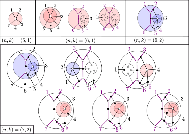
Figure 24. Some BCFW collections in terms of plabic graphs. For $(n,k)=(5,1)$ and $(n,k)=(6,2)$, there is a unique BCFW collection which contains the unique BCFW cell $\operatorname{Gr}^{>0}_{1,\{1,2,3,4,5\}}$ and $\operatorname{Gr}_{0,\{6,1,2\}}\bowtie\operatorname{Gr}_{1,\{2,3,4,5,6\}}$, respectively. For $(n,k)=(6,1)$, we show a BCFW collection where $\mathcal{T}_{pre}$ and each $\mathcal{T}_{k_{L},k_{R},b,n}$ consists of a single cell. For $(n,k)=(7,2)$ we show a $6$-element BCFW collection.

Theorem 12.3 (BCFW tilings).

Let $\{S_{1},\dots,S_{\ell}\}$ be a BCFW collection of cells for $\mathcal{A}_{n,k,4}$. Then for all $Z$, the corresponding collection of tiles $\{Z_{S_{1}},\dots,Z_{S_{\ell}}\}$ is a tiling of the amplituhedron $\mathcal{A}_{n,k,4}(Z)$, which we refer to as a BCFW tiling.

	$0$	$1$	$2$	$3$	$4$	$5$
$5$	$1$	$1$
$6$	$1$	$2$	$1$
$7$	$1$	$7$	$7$	$1$
$8$	$1$	$40$	$2624$	$40$	$1$
$9$	$1$	$297$	$>10^{7}$	$>10^{7}$	$297$	$1$

Table 2. Number of BCFW tilings of $\mathcal{A}_{n,k,4}(Z)$

Theorem 12.3 is a special case of the more general Theorem 12.6, which we will prove below.

Definition 12.4.

A collection $\mathcal{T}$ of $4k$-dimensional BCFW cells in $\operatorname{Gr}_{k,n}^{\geq 0}$ is called a quasi-BCFW collection of cells for $\mathcal{A}_{n,k,4}$ if there is a decomposition

$$\mathcal{T}=\mathcal{T}_{\operatorname{pre}}\sqcup\bigsqcup_{k_{L},k_{R},b}{\mathcal{T}_{k_{L},k_{R},b,n}},$$

where

• $b$ ranges from $b_{min}$ to $n-3-k_{R}$, and $b_{min},k_{L},k_{R}$ as in 12.1,

• $\mathcal{T}_{pre}=\{\operatorname{pre}_{d}(S^{i})|i\in\mathcal{F}\},$ where the collection $\{S^{i}|i\in\mathcal{F}\}$ gives a tiling of $\mathcal{A}_{[n]\setminus\{d\},k,4}$ for all $Z$,

• $\mathcal{T}_{k_{L},k_{R},b,n}$ has either of the following forms:

  • $\{S^{i,j}_{L}\bowtie S_{R}^{i}\ |\ i\in\mathcal{D},j\in\mathcal{E}_{i}\}$, where the collection $\{S_{R}^{i}\subset\operatorname{Gr}_{k_{R},N_{R}}^{\geq 0}\ |\ i\in\mathcal{D}\}$ gives a tiling of $\mathcal{A}_{N_{R},k_{R},4}$ for all $Z$, and for every $i$ the collection $\{S_{L}^{i,j}\subset\operatorname{Gr}_{k_{L},N_{L}}^{\geq 0}\ |\ j\in\mathcal{E}_{i}\}$ gives a tiling of $\mathcal{A}_{N_{L},k_{L},4}$ for all $Z$,

  • $\{S^{i}_{L}\bowtie S_{R}^{i,j}\ |\ S^{i}_{L}\subset\operatorname{Gr}_{k_{L},N_{L}}^{\geq 0},S_{R}^{i,j}\subset\operatorname{Gr}_{k_{R},N_{R}}^{\geq 0},i\in\mathcal{D},j\in\mathcal{E}_{j}\},$ and the conditions on the right and left side in the above point are interchanged.

  In the first case we say that $\mathcal{T}_{k_{L},k_{R},b,n}$ is fibred on the right side, and in the second we say it is fibred on the left side.

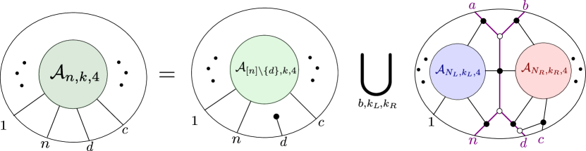
Figure 25. BCFW tiling for $\mathcal{A}_{n,k,4}$. On the right hand side: the first term is obtained by tiling $\mathcal{A}_{[n]\setminus\{d\},k,4}$ (from $\mathcal{T}_{pre}$); the second term is the union over $b,k_{L},k_{R}$ as in Definition 12.4 of the collections of tiles obtained by tiling $\mathcal{A}_{N_{L},k_{L},4}$ and $\mathcal{A}_{N_{R},k_{R},4}$ independently (from $\mathcal{T}_{k_{L},k_{R},b,n}$).

Remark 12.5.

Definition 12.4 is similar to Definition 12.2. However, while the tiles involved in Definition 12.4 are all BCFW tiles, their collection does not need to be produced via the recursion in Definition 12.2, but instead is obtained from tilings of amplituhedra with smaller $n$ and $k$.

Theorem 12.6.

Let $\mathcal{T}=\{S_{1},\dots,S_{\ell}\}$ be a quasi-BCFW collection of cells for $\mathcal{A}_{n,k,4}$. Then for all $Z$, the corresponding collection of tiles $\{Z_{S_{1}},\dots,Z_{S_{\ell}}\}$ is a tiling of the amplituhedron $\mathcal{A}_{n,k,4}({Z})$.

Our starting point for proving Theorem 12.6 is the following theorem, proven in [ELT21, Theorem 9.5, Lemma 9.7] and the comment after the proof of [ELT21, Proposition 9.9].

Theorem 12.7.

Let $Z\in\operatorname{Mat}_{n,k+4}^{>0}$ and

$$C_{\operatorname{pre}}:=\operatorname{pre}_{d}(\operatorname{Gr}^{>0}_{k,[n]\setminus\{d\}})\text{ and }C_{k_{L},k_{R},b,n}:=\operatorname{Gr}^{>0}_{k_{L},N_{L}}\bowtie\operatorname{Gr}^{>0}_{k_{R},N_{R}}.$$

Then the sets

$$\{\tilde{Z}(C_{\operatorname{pre}})\}\cup\{\tilde{Z}(C_{k_{L},k_{R},b,n})\ |\ k_{L},k_{R}\geq 0,\,k_{L}+k_{R}=k-1,\,b_{min}\leq b\leq n-3-k_{R}\}$$

are pairwise disjoint and their union is dense in $\mathcal{A}_{n,k,4}(Z).$

In particular, on $\tilde{Z}(C_{\operatorname{pre}})$ all twistor coordinates $\langle\!\langle i,i+1,n-2,n\rangle\!\rangle$ with $i\in[1,n-4]$ are positive, while on each $\tilde{Z}(C_{k_{L},k_{R},b,n})$ at least one such twistor coordinate is negative. In addition, for all $b\neq b^{\prime}$ the quadratic functionaries $\langle\!\langle b^{\prime}-1,b^{\prime},n\,|\,n-2,d\,|\,b,b-1,n\rangle\!\rangle$ have opposite signs on $\tilde{Z}(C_{k_{L},k_{R},b,n})$ and $\tilde{Z}(C_{k_{L},k_{R},b^{\prime},n}).$

Definition 12.8.

We say that two open tiles $Z_{S_{1}}^{\circ},Z_{S_{2}}^{\circ}$ are separated by a family $F_{1},\ldots,F_{N}$ of functionaries if each $F_{i}$ has a strong sign on one of $Z_{S_{1}}^{\circ},Z_{S_{2}}^{\circ},$ and, there are two disjoint sets $A,B\subset\{-1,0,1\}^{N}$ such that for all $Z$

$$(\operatorname{sgn}F_{1}(Y),\operatorname{sgn}F_{2}(Y),\ldots,\operatorname{sgn}F_{N}(Y))\in A\text{ for all }Y\in Z_{S_{1}}^{\circ},$$

$$\text{while }(\operatorname{sgn}F_{1}(Y),\operatorname{sgn}F_{2}(Y),\ldots,\operatorname{sgn}F_{N}(Y))\in B\text{ for all }Y\in Z_{S_{2}}^{\circ}.$$

Remark 12.9.

If $Z_{S_{1}}^{\circ},Z_{S_{2}}^{\circ}$ are separated by a family of functionaries, then $Z_{S_{1}}^{\circ}\cap Z_{S_{2}}^{\circ}=\emptyset$ for all $Z.$

Corollary 12.10.

Two BCFW tiles $Z_{S_{1}},Z_{S_{2}}$ satisfy $Z_{S_{1}}^{\circ}\cap Z_{S_{2}}^{\circ}=\emptyset$ for all $Z$ if and only if they are separated by a family of functionaries.

This corollary is an immediate consequence of Remark 12.9, and Theorem 7.7 and its proof, as we can take the collection of coordinates functionaries for the two open tiles $Z_{S_{1}}^{\circ},Z_{S_{2}}^{\circ}$ as the list of functionaries.

As we already proved BCFW cells give tiles in Theorem 7.7, the following two results are enough to complete the proof of Theorem 12.6.

Proposition 12.11.

Let $\mathcal{T}$ be a quasi-BCFW collection of cells for $\mathcal{A}_{n,k,4}$. Then $Z_{S_{1}}^{\circ}\cap Z_{S_{2}}^{\circ}=\emptyset$, for any pair of cells $S_{1},S_{2}$ in $\mathcal{T}$.

Proposition 12.12.

Let $\mathcal{T}$ be a quasi-BCFW collection of cells for $\mathcal{A}_{n,k,4}$. Then $\mathcal{A}_{n,k,4}(Z)=\bigcup_{S\in\mathcal{T}}Z_{S}.$

In the rest of the section, we proceed with proving Proposition 12.11, and then Proposition 12.12.

Proof of Proposition 12.11.

By the definition of a BCFW collection, every $S\in\mathcal{T}$ belongs to either $\mathcal{T}_{\operatorname{pre}}$ or to $\mathcal{T}_{k_{L},k_{R},b,n}.$

Case (1): Consider $S_{1},S_{2}\in\mathcal{T}.$ If $S_{1},S_{2}\in\mathcal{T}$ both belong to $\mathcal{T}_{\operatorname{pre}},$ then they can be written as

$$S_{1}=\operatorname{pre}_{d}(S^{\prime}_{1}),\text{ and }S_{2}=\operatorname{pre}_{d}(S^{\prime}_{2}),$$

where by construction and Corollary 12.10 there is a family of functionaries $F_{1},\ldots,F_{n}$ separating $S^{\prime}_{1},S^{\prime}_{2}$. The same functionaries are easily seen to separate $S_{1},S_{2}$ using Theorem 11.2. Hence the claim follows by Corollary 12.10.

Case (2): If $S_{1},S_{2}\in\mathcal{T}_{k_{L},k_{R},b,n}$, then without loss of generality,

$$S_{1}=S_{L}^{i,j}\bowtie S_{R}^{i}\text{ and }S_{2}=S_{L}^{i^{\prime},j^{\prime}}\bowtie S_{R}^{i^{\prime}},$$

where $\{S_{R}^{i}\}$ gives a tiling of $\mathcal{A}_{N_{R},k_{R},4}(Z_{R})$ for all $Z_{R}$ and $\{S_{L}^{i,j}\},~{}\{S_{L}^{i^{\prime},j^{\prime}}\}$ for fixed $i,i^{\prime}$ gives a tiling of $\mathcal{A}_{N_{L},k_{L},4}(Z_{L})$ for all $Z_{L}$.

Since $S_{1}\neq S_{2}$ either $i\neq i^{\prime}$ or $i=i^{\prime}$ but $j\neq j^{\prime}.$ We treat the first case, the second is treated similarly. By Corollary 12.10, $Z_{S_{R}^{i}}^{\circ},Z_{S_{R}^{i^{\prime}}}^{\circ}$ can be separated by a family $F_{1},\ldots,F_{N}$ of functionaries. Using Item 2, Item 3 of Theorem 11.3, we will show that $Z_{S_{1}}^{\circ}$ and $Z_{S_{2}}^{\circ}$ can be separated by the family $\Psi({F}_{1}),\ldots,\Psi({F}_{N})$ of functionaries and so are disjoint for all $Z$ by Corollary 12.10. Without loss of generality, let $F_{1},\ldots,F_{M}$ have a strong sign $+$ on $Z_{S_{R}^{i}}^{\circ}$ and $F_{M+1},\ldots,F_{N}$ have a strong sign $+$ on $Z_{S_{R}^{i^{\prime}}}^{\circ}.$ This means that on $Z_{S_{R}^{i}}^{\circ}$ the signs of $(F_{1},\ldots,F_{N})$ are of the form

$$(+1,\ldots,+1,s_{M+1},\ldots,s_{N}),~{}\text{where }(s_{M+1},\ldots,s_{N})\in U\subseteq\{\pm 1,0\}^{\{M+1,\ldots,N\}},$$

while on $Z_{S_{R}^{i^{\prime}}}^{\circ}$ these signs are all of the form

$$(s_{1},\ldots,s_{M},+1,\ldots,+1),~{}\text{where }(s_{1},\ldots,s_{M})\in V\subseteq\{\pm 1,0\}^{\{1,\ldots,M\}}.$$

Since $F_{1},\dots,F_{N}$ is separating, at most one of $U,V$ contains the all $+1$ vector. By  Item 2 and Item 3 of Theorem 11.3, on every point of $Z_{S_{1}}^{\circ}$ the promotions $(\Psi(F_{1}),\ldots,\Psi(F_{N}))$ have a sign vector of the form

$$(+1,\ldots,+1,s_{M+1},\ldots,s_{N}),~{}\text{where }(s_{M+1},\ldots,s_{N})\in\operatorname{cl}(U)\subseteq\{\pm 1,0\}^{\{M+1,\ldots,N\}},$$

while on every point of $Z_{S_{2}}^{\circ}$ the sign vector is of the form

$$(s_{1},\ldots,s_{M},+1,\ldots,+1),~{}\text{where }(s_{1},\ldots,s_{M})\in\operatorname{cl}(V)\subseteq\{\pm 1,0\}^{\{1,\ldots,M\}}.$$

Notice that a sign vector is simultaneously of the form $(+1,\ldots,+1,s_{M+1},\ldots,s_{N})$ and of the form $(s_{1},\ldots,s_{M},+1,\ldots,+1)$ if and only if it is the all $+1$ vector. At most one of $\operatorname{cl}(U),\operatorname{cl}(V)$ contains the all $+1$ vector, since at most one of $U,V$ contains the all $+1$ vector.

Thus, the sets

$$\{(+1,\ldots,+1,s_{M+1},\ldots,s_{N}):(s_{M+1},\ldots,s_{N})\in\text{cl}(U)\},$$

$$\{(s_{1},\ldots,s_{M},+1,\ldots,+1):(s_{1},\ldots,s_{M})\in\text{cl}(V)\}$$

do not intersect.

Case (3): Suppose $S_{1}$ and $S_{2}$ belong to different sets among $\mathcal{T}_{\operatorname{pre}},\{\mathcal{T}_{k_{L},k_{R},b}\}_{k_{L},k_{R},b}$. Denote these sets by $\mathcal{T}_{1},\mathcal{T}_{2}$ respectively, and let $C_{1},C_{2}$ such that $C_{i}=C_{\operatorname{pre}}$ if $\mathcal{T}_{i}=\mathcal{T}_{\operatorname{pre}}$, and $C_{i}=C_{k_{L},k_{R},b,n}$ if $\mathcal{T}_{i}=\mathcal{T}_{k_{L},k_{R},b,n}$ ($C_{pre}$ and $C_{k_{L},k_{R},b,n}$ are as in Theorem 12.7.)

Assume towards contradiction that for some $Z$ the intersection $Z_{S_{1}}^{\circ}\cap Z_{S_{2}}^{\circ}$ is non empty. Then, since $Z_{S_{1}}^{\circ},Z_{S_{2}}^{\circ}$ are open (Corollary 11.16), also their intersection $U\neq\emptyset$ is open. Lemma 12.13 below shows that also $\tilde{Z}(C_{1}),\tilde{Z}(C_{2})$ are open. Since

$$Z_{S_{1}}^{\circ}\subseteq\overline{\tilde{Z}(C_{1})},~{}Z_{S_{2}}^{\circ}\subseteq\overline{\tilde{Z}(C_{2})},$$

this implies $U$ is contained in $\overline{\tilde{Z}(C_{1})}\cap\overline{\tilde{Z}(C_{2})},$ and hence intersects ${\tilde{Z}(C_{1})}\cap{\tilde{Z}(C_{2})}$ in an open nonempty set. But this contradicts Theorem 12.7.

∎

Lemma 12.13.

Let $S_{L}^{\triangleright},~{}S_{R}^{\triangleleft}$ be as in 11.7. Then:

• the sets $Z_{S_{L}^{\triangleright}}^{\circ}$ and $Z_{S_{R}^{\triangleleft}}^{\circ}$ are open;

• the sets $\tilde{Z}(C_{\operatorname{pre}})$ and $\tilde{Z}(C_{k_{L},k_{R},b,n})$ are open.

Proof.

We start with the first statement. We prove it for $Z_{S_{R}^{\triangleleft}}^{\circ},$ the proof for $Z_{S_{L}^{\triangleright}}^{\circ}$ is similar. We will show that the amplituhedron map is submersive on $S_{R}^{\triangleleft},$ and since submersions are open it will prove our claim.

Note that for $|N_{L}|\leq k_{L}+4$, $S_{R}^{\triangleleft}$ is a BCFW cell, hence $\tilde{Z}|_{S_{R}^{\triangleleft}}$ is open and submersive by Corollary 11.16.

Let $|N_{L}|>k_{L}+4$ and denote $W_{L}=\text{Span}(Z_{i}:i\in N_{L}),$ $d=\dim(W_{L}).$ Since every $k+4$ rows of $Z$ are linearly independent, $d=\min(N_{L},k+4)$

Let $\pi:F\to\operatorname{Gr}_{k_{L}}(W_{L})$ be the fiber bundle whose fiber over $W\in\operatorname{Gr}_{k_{L}}(W_{L})$ is

$$F_{W}=\pi^{-1}(W)=\operatorname{Gr}_{k_{R}+1}(\mathbb{R}^{k+4}/W).$$

The amplituhedrom map $\tilde{Z}:S_{R}^{\triangleleft}\to\operatorname{Gr}_{k,k+4}$ decomposes as

$$S_{R}^{\triangleleft}\to F\to\operatorname{Gr}_{k,k+4},$$

where the map $\Phi:F\to\operatorname{Gr}_{k,k+4}$ is given by

$$\Phi(U,W)=U+W,$$

and the map $\Xi:S_{R}^{\triangleleft}\to F$ is given by

$$\Xi(V)=(\tilde{Z}(V)/(V_{L}Z),V_{L}Z),$$

where $V_{L}=V\cap\text{Span}(\mathbf{e}_{i}:i\in N_{L}).$

We will show that these maps are well defined and submersive. This will imply that also their composition, $\tilde{Z}|_{S_{R}^{\triangleleft}}$ is a submersion.
The map $\Phi$: $\Phi$ is well defined, since if $U_{1},U_{2}$ are different liftings of a $(k_{R}+1)$-subspace of $\mathbb{R}^{k+4}/W$ to $k$-spaces $U^{\prime}_{1},U^{\prime}_{2}\subseteq\mathbb{R}^{k+4},$ then

$$U^{\prime}_{1}+W=U^{\prime}_{2}+W\in\operatorname{Gr}_{k,k+4}.$$

It surjective, since any $k-$space $V\subseteq\mathbb{R}^{k+4}$ intersects $W_{L}$ in a subspace of dimension at least $d-4\geq k_{L}.$ Thus we can decompose $V$ (not uniquely) as $U+W$ where $W$ is a $k_{L}-$space in $W_{L}\cap V.$ $\Phi$ is then seen to be everywhere submersive, by standard arguments.
The map $\Xi$: Let $V$ be an element of $S_{R}^{\triangleleft},$ by the proof of Proposition 10.2 and Remark 10.3, $V$ can be written uniquely as

$$V=V_{L}\oplus V_{R},$$

where $V_{L}\in\operatorname{pre}_{b+1,\ldots,d-1}\operatorname{Gr}^{>0}_{k_{L},N_{L}}$ and $V_{R}$ belongs to the BCFW cell $S^{\prime}_{R}$ of $\operatorname{pre}_{1,\ldots,a-1}\operatorname{Gr}^{\geq 0}_{k_{R}+1,N_{R}}$ obtained by applying the upper BCFW map with indices $a,b,c,d,n$ to $S_{R},$ and then adding zero columns.

Let $Y_{L}:=V_{L}Z$, then $Y_{L}\subseteq W_{L}.$ In addition, $V_{L}\in\operatorname{pre}_{b+1,\ldots,d-1}\operatorname{Gr}^{>0}_{k_{L},N_{L}}\subseteq\operatorname{Gr}^{\geq 0}_{k_{L},n}$. On $\operatorname{Gr}^{\geq 0}_{k_{L},n},$ right multiplication by the positive matrix $Z$ is just the amplituhedron map from $\operatorname{Gr}^{\geq 0}_{k_{L},n}$ to $\operatorname{Gr}_{k_{L},k+4}$. Hence $Y_{L}\in\mathcal{A}_{n,k_{L},k+4-k_{L}}(Z)$, so in particular $Y_{L}$ is of dimension $k_{L}$ and $Y_{L}\in\operatorname{Gr}_{k_{L}}(W_{L})$.

Since $\Xi(V)=(Y/Y_{L},Y_{L}),$ $\Xi$ indeed maps $S_{R}^{\triangleleft}$ to $F.$

Let’s denote by $T_{p}M$ the tangent space of the differentiable manifold $M$ at the point $p$. We can conclude that $\Xi$ is a submersion if we show that:

1. at $V\in S_{R}^{\triangleleft}$, the $V_{L}$ directions of $T_{V}S_{R}^{\triangleleft}$ surject on the base directions $T_{Y_{L}}\operatorname{Gr}_{k_{L}}(W_{L})$;

2. at $V\in S_{R}^{\triangleleft}$, the $V_{R}$ directions surject on the fiber directions $T_{Y/Y_{L}}\operatorname{Gr}_{k_{R}+1}(\mathbb{R}^{k+4}/Y_{L})$.

Item 1 can be proved by using standard arguments. We will now prove Item 2.

In order to show that $\Xi$ is a submersion, we will show that at $V\in S_{R}^{\triangleleft},$ the $V_{L}$ directions of $T_{V}S_{R}^{\triangleleft}$ surject on the base directions $T_{Y_{L}}\operatorname{Gr}_{k_{L}}(W_{L}),$ while the $V_{R}$ directions subrject on the fiber directions $T_{Y/Y_{L}}\operatorname{Gr}_{k_{R}+1}(\mathbb{R}^{k+4}/Y_{L}).$

Let us fix $V_{L}$ and note that

$$Y_{R}:=Y/Y_{L}\subseteq\mathbb{R}^{k+4}/Y_{L}$$

is a $k_{R}+1$ space, which lies in the image of $S^{\prime}_{R}$ under the map

(35) $$\operatorname{Gr}^{\geq 0}_{k_{R}+1,N_{R}}\to\operatorname{Gr}_{k_{R}+1}(\mathbb{R}^{k+4}/Y_{L}),$$

obtained by the right multiplication of $Z^{V_{L}},$ whose rows are

$$Z_{i}/Y_{L},~{}i=a,b,b+1,\ldots,n.$$

Once fixing an identification of $\mathbb{R}^{k+4}/Y_{L}$ with $\mathbb{R}^{(k_{R}+1)+4},$ this map becomes the amplituhedron map, as long as $Z^{V_{L}}$ is a positive matrix under this identification. Note that different identifications leave the maximal minors of $Z^{V_{L}}$ and the twistor coordinates of a point in $\operatorname{Gr}_{k_{R}+1}(\mathbb{R}^{k+4}/Y_{L})$ invariant, up to a common multiplicative scalar. In particular, whether a functionary vanishes at a given point is independent of the identification with $\mathbb{R}^{k_{R}+5}.$

We now show that all Plücker coordinates of $Z^{V_{L}}$ have the same sign, hence there is an identification which makes this matrix positive. Using linear algebra, it is easy to show that the Plücker coordinates $\langle I\rangle_{Z^{V_{L}}}$ equal (up to multiplication of a common scalar) the determinants $\det(Y^{\prime}_{L}|Z^{\prime}_{I})$ of the $(k+4)\times(k+4)$ matrix obtained by stacking $Y^{\prime}_{L}=C_{L}Z$, where $C_{L}$ is a matrix representative of $V_{L}$, with a lift $Z^{\prime}_{I}$ of the rows $I$ of $Z^{V_{L}}$ to $\mathbb{R}^{k+4}$. Here $I$ runs over subsets of $\{a,\ldots,n\}$ of size $k_{R}+5=k+4-k_{L}$.

The determinant $\det(Y_{L}|Z^{\prime}_{I})$ can be expressed as the determinant of the matrix $C^{\prime}_{L}Z,$ where $C^{\prime}_{L}$ is the $(k+4)\times n$ matrix whose first $k_{L}$ rows are $C_{L},$ and the remaining rows are the standard basis elements $\mathbf{e}_{i},~{}i\in I.$ $C^{\prime}_{L}$ is non-negative, $Z$ is positive, and by Lemma 2.16 the determinant of $C^{\prime}_{L}Z,$ is positive. Hence $\det(Y_{L}|Z^{\prime}_{I})$ and the Plücker coordinates $\langle I\rangle_{Z^{V_{L}}}$ are positive.

We can now show that the map in Equation 35 is submersive: its inverse map is smooth near $Y/Y_{L},$ since we can run the same pre-image algorithm of Theorem 7.7 for the cell $S^{\prime}_{R},$ in analogy with the usual amplituhedron map. The algorithm does not stop as long as certain functionaries are nowhere zero, see the proof of Theorem 7.7. Recall that whether a functionary is zero is independent of the identification with $\mathbb{R}^{k_{R}+5}.$

The proof regarding $\tilde{Z}(C_{k_{L},k_{R},b,n})$ is similar to the one of $Z_{S_{R}^{\triangleleft}}^{\circ}$, but one can use standard arguments to prove both the analogue of Item 1 and Item 2.

Finally, we complete the proof regarding $C_{\operatorname{pre}}$. The fact that the amplituhedron map from $\operatorname{Gr}^{>0}_{k,[n]\setminus\{n-1\}}$ to $\operatorname{Gr}_{k,k+4}$ is a submersion was shown in [ELT21, Theorem 1.5]. It is straightforward to conclude that also the amplituhedron map restricted to $C_{\operatorname{pre}}=\operatorname{pre}_{n-1}\operatorname{Gr}^{>0}_{k,[n]\setminus\{n-1\}}$ submerses.

∎

In order to prove Proposition 12.12, we need the following results from [BH19, Proposition 3.3, Corollary 3.2, Lemma 3.1]:

Theorem 12.14.

Let $\{S_{\ell}\}_{\ell\in\mathcal{C}}$ be a collection of positroid cells in $\operatorname{Gr}^{\geq 0}_{k,[n]\setminus\{i\}}$.

1. If $\{Z_{S_{\ell}}\}_{\ell\in\mathcal{C}}$ tiles $\tilde{Z}(\operatorname{Gr}_{k,[n]\setminus\{i\}}^{\geq 0})$ for all $Z$, then $\{Z_{\operatorname{pre}_{i}(S_{\ell})}\}_{\ell\in\mathcal{C}}$ tiles ${\tilde{Z}(\operatorname{pre}_{i}(\operatorname{Gr}^{\geq 0}_{k,[n]\setminus\{i\}}))}$ for all $Z$

2. If $\{Z_{S_{\ell}}\}_{\ell\in\mathcal{C}}$ tiles $\tilde{Z}(\operatorname{Gr}_{k,[n]\setminus\{i\}}^{\geq 0})$ for all $Z,$ then $\{Z_{\operatorname{inc}_{i}(S_{\ell})}\}_{\ell\in\mathcal{C}}$ tiles $\tilde{Z}({\operatorname{inc}_{i}(\operatorname{Gr}^{\geq 0}_{k+1,[n]\setminus\{i\}})})$ for all $Z$

3. Let $\{S_{j}\}_{j\in\mathcal{D}}$ be a collection of positroid cells in $\operatorname{Gr}_{k,n}^{\scriptscriptstyle\geq 0}$. If $\{Z_{S_{j}}\}_{j\in\mathcal{D}}$ tiles $\mathcal{A}_{n,k,4}(Z)$ for all $Z,$ then $\{Z_{\operatorname{cyc}_{i}(S_{j})}\}_{j\in\mathcal{D}}$ tiles $\mathcal{A}_{n,k,4}(Z)$ for all $Z.$

4. Let $S$ be a positroid cell in $\operatorname{Gr}_{k,n}^{\scriptscriptstyle\geq 0},$ and let $S_{1},\ldots,S_{r}$ be positroid cells contained in $\overline{S}.$
   If the union of $Z_{S_{1}},\ldots,Z_{S_{r}}$ equals $Z_{S}$ for all $Z$, then for any $j\in[n]$ we have:

   $$Z_{x_{j}(\mathbb{R}_{+}).S}=\bigcup_{i=1}^{r}{Z_{x_{j}(\mathbb{R}_{+}).S_{i}}}\qquad\text{and}\qquad Z_{y_{j}(\mathbb{R}_{+}).S}=\bigcup_{i=1}^{r}Z_{y_{j}(\mathbb{R}_{+}).S_{i}},\quad\mbox{for all }Z.$$

Recall from 11.7 the definition of $S^{\triangleright}$ and $S^{\triangleleft}$.

Lemma 12.15.

Let $\mathcal{C}$ be a collection of BCFW cells. If $\{Z_{S}\}_{S\in\mathcal{C}}$ tiles $\mathcal{A}_{N_{L},k_{L},4}$ (respectively, $\mathcal{A}_{N_{R},k_{R},4}$), then $\{Z_{S^{\triangleright}}\}_{S\in\mathcal{C}}$ (respectively, $\{Z_{S^{\triangleleft}}\}_{S\in\mathcal{C}}$) covers $Z_{C_{k_{L},k_{R},b,n}}$ for all $Z$.

Proof.

By Lemma 11.8 this statement follows by subsequent applications of Theorem 12.14. More specifically, there is a sequence $\mathfrak{s}$ of operations of the form $\operatorname{pre}_{i},\operatorname{inc}_{i},x_{i}(\mathbb{R}_{+}),y_{i}(\mathbb{R}_{+})$, such that for each $S\in\mathbb{C}$ $\mathfrak{s}.S=S^{\triangleleft}$ and also $\mathfrak{s}.\operatorname{Gr}^{\geq 0}_{k_{R},N_{R}}=\operatorname{Gr}^{\geq 0}_{k_{L},N_{L}}\bowtie\operatorname{Gr}^{\geq 0}_{k_{R},N_{R}}$. This means that $Z_{\mathfrak{s}.\operatorname{Gr}^{\geq 0}_{k_{R},N_{R}}}=\cup_{S\in\mathbb{C}}Z_{\mathfrak{s}.S}$. An analogous argument works for $S^{\triangleright}$. ∎

Lemma 12.16.

For every BCFW cell $S_{R}$ in $\operatorname{Gr}^{\geq 0}_{k_{R},N_{R}},$ and every BCFW cell $S_{L}$ in $\operatorname{Gr}^{\geq 0}_{k_{L},N_{L}},$

$$\overline{Z_{S_{L}^{\triangleright}}^{\circ}\cap Z_{S_{R}^{\triangleleft}}}=\overline{Z_{S_{L}^{\triangleright}}\cap Z_{S_{R}^{\triangleleft}}^{\circ}}=\overline{Z_{S_{L}^{\triangleright}}^{\circ}\cap Z_{S_{R}^{\triangleleft}}^{\circ}}\subseteq Z_{S_{L}\bowtie S_{R}}$$

Proof.

The equalities hold since $Z_{S_{L}^{\triangleright}}^{\circ},~{}Z_{S_{R}^{\triangleleft}}^{\circ}$ are open, by Lemma 12.13. We now show the inclusion. Let $F_{1},\ldots,F_{5k}$ be the coordinate functionaries of $Z_{S_{L}\bowtie S_{R}}^{\circ}$ where the first $5k_{L}$ are the promotions of the coordinate functionaries of $S_{L},$ the last $5k_{R}$ are the promotions of the coordinate functionaries of $S_{R}$ and the remaining $5$ are the (signed) twistors introduced in the $k$-th step-tuple. By Lemma 11.4, the $5$ (signed) twistors are positive on $Z_{S_{L}\bowtie S_{R}}^{\circ},Z_{S_{L}^{\triangleright}}^{\circ},Z_{S_{R}^{\triangleleft}}^{\circ}.$ By Theorem 11.3, the first $5k_{L}$ are positive on $Z_{S_{L}\bowtie S_{R}}^{\circ},Z_{S_{L}^{\triangleright}}^{\circ}$ and the last $5k_{R}$ are positive on $Z_{S_{L}\bowtie S_{R}}^{\circ},Z_{S_{R}^{\triangleleft}}^{\circ}.$ By Theorem 7.7 every point for which all the $F_{i}$ are positive belongs to $Z_{S_{L}\bowtie S_{R}}^{\circ}.$ Thus, every point of $Z_{S_{L}^{\triangleright}}^{\circ}\cap Z_{S_{R}^{\triangleleft}}^{\circ}$ belongs to $Z_{S_{L}\bowtie S_{R}}^{\circ}.$ We finish by taking closures. ∎

Proof of Proposition 12.12.

By our assumptions, and Item 1 of Theorem 12.14, , $\mathcal{T}_{\operatorname{pre}}$ gives a tiling of $Z_{\overline{C}_{\operatorname{pre}}},$ for all $Z$. We will now show that the collection $\{Z_{S}\}_{S\in\mathcal{T}_{k_{L},k_{R},b,n}}$ covers the subspace $Z_{{C}_{k_{L},k_{R},b,n}}$. The result will then follow from Theorem 12.7.

Fix $k_{L},k_{R},b,n$ and suppose without loss of generality that $\mathcal{T}_{k_{L},k_{R},b,n}$ is fibred on the right side:

$$\mathcal{T}_{k_{L},k_{R},b,n}=\{S^{i,j}_{L}\bowtie S_{R}^{i}\ |\ i\in\mathcal{D},j\in\mathcal{E}_{i}\},$$

where the collection $\{Z_{S_{R}^{i}}\ |\ i\in\mathcal{D}\}$ tiles of $\mathcal{A}_{N_{R},k_{R},4}(Z_{R})$ for all $Z_{R}$ and for every $i$ the collection $\{Z_{S_{L}^{i,j}}\ |\ j\in\mathcal{E}_{i}\}$ covers $\mathcal{A}_{N_{L},k_{L},4}(Z_{L})$ for all $Z_{L}$. By Lemma 12.15, $\{Z_{(S_{R}^{i})^{\triangleleft}}\ |\ i\in\mathcal{D}\}$ covers $Z_{C_{k_{L},k_{R},b,n}}$ for all $Z$. Similarly, for every $i,$ $\{(S_{L}^{i,j})^{\triangleright}\ |\ j\in\mathcal{E}_{i}\}$ gives a tiling of $Z_{C_{k_{L},k_{R},b,n}}$ for all $Z$. Thus, for all $Z,$ and every $i\in\mathcal{D}.$

$$Z_{(S_{R}^{i})^{\triangleleft}}=\overline{Z_{(S_{R}^{i})^{\triangleleft}}^{\circ}}=\overline{\bigcup_{j\in\mathcal{E}_{i}}Z_{(S_{R}^{i})^{\triangleleft}}^{\circ}\cap Z_{(S_{L}^{i;j})^{\triangleright}}}\subseteq\overline{\bigcup_{j\in\mathcal{E}_{i}}Z_{S_{L}^{i,j}\bowtie S_{R}^{i}}}=\bigcup_{j\in\mathcal{E}_{i}}Z_{S_{L}^{i,j}\bowtie S_{R}^{i}},$$

where the inclusion is by Lemma 12.16 and the last equality uses that $Z_{S}$ are closed sets. Therefore

$$Z_{C_{k_{L},k_{R},b,n}}\subseteq\bigcup_{i\in\mathcal{D},j\in\mathcal{E}_{i}}Z_{S_{L}^{i,j}\bowtie S_{R}^{i}}.$$

This completes the proof. ∎

Appendix A Background on plabic graphs

In [Pos06], Postnikov classified the cells of the positive Grassmannian, using equivalence classes of reduced plabic graphs, and decorated (or affine) permutations. Here we review some of this technology, following [FWZb], [Pos06], and [PSW07].

Definition A.1 (Plabic graphs).

A planar bicolored graph (or “plabic graph”) is a planar graph $G$ properly embedded into a closed disk, such that each internal vertex is colored black or white; each internal vertex is connected by a path to some boundary vertex; there are (uncolored) vertices lying on the boundary of the disk labeled $1,\dots,n$ for some positive $n$; and each of the boundary vertices is incident to a single edge. See Figure 26 for an example.

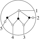
Figure 26. A plabic graph

If $G$ has an internal leaf which is incident to a boundary vertex, we call this a lollipop. We will require that our plabic graphs have no internal leaves except for lollipops.

There is a natural set of local transformations (moves) of plabic graphs:

(M1) Square move (or urban renewal). If a plabic graph has a square formed by four trivalent vertices whose colors alternate, then we can switch the colors of these four vertices.

(M2) Contracting/expanding a vertex. Two adjacent internal vertices of the same color can be merged or unmerged.

(M3) Middle vertex insertion/removal. We can remove/add degree $2$ vertices.

See Figure 27 for depictions of these three moves.

       

Figure 27. Local moves (M1), (M2), (M3) on plabic graphs.

Definition A.2.

Two plabic graphs are move-equivalent if they can be obtained from each other by moves (M1)-(M3). The move-equivalence class of a given plabic graph $G$ is the set of all plabic graphs which are move-equivalent to $G$. A plabic graph is called reduced if there is no graph in its move-equivalence in which there is a bubble, that is, two adjacent vertices $u$ and $v$ which are connected by more than one edge.

Definition A.3 (Decorated permutations).

A decorated permutation on $[n]$ is a bijection $\pi:[n]\to[n]$ whose fixed points are each coloured either black (loop) or white (coloop). We denote a black fixed point $i$ by $\pi(i)=\underline{i}$, and a white fixed point $i$ by $\pi(i)=\overline{i}$. An anti-excedance of the decorated permutation $\pi$ is an element $i\in[n]$ such that either $\pi^{-1}(i)>i$ or $\pi(i)=\overline{i}$. We say that a decorated permutation on $[n]$ is of type $(k,n)$ if it has $k$ anti-excedances.

Definition A.4.

Let $G$ be a reduced plabic graph as above with boundary vertices $1,\dots,n$. For each boundary vertex $i\in[n]$, we follow a path along the edges of $G$ starting at $i$, turning (maximally) right at every internal black vertex, and (maximally) left at every internal white vertex. This path ends at some boundary vertex $\pi(i)$. By [FWZb, Proposition 7.4.22], the fact that $G$ is reduced implies that each fixed point of $\pi$ is attached to a lollipop; we color each fixed point by the color of its lollipop. In this way we obtain the decorated permutation $\pi_{G}=\pi$ of $G$. We say that $G$ is of type $(k,n)$, where $k$ is the number of anti-excedances of $\pi_{G}$.

The decorated trip permutation of the plabic graph $G$ of Figure 26 is $\pi_{G}=(3,4,5,1,2)$, which has $k=2$ anti-excedances.

Theorem A.5 (Fundamental theorem of reduced plabic graphs).

[FWZb, Theorem 7.4.25] [Pos06] Let $G$ and $G^{\prime}$ be reduced plabic graphs. The following statements are equivalent:

• $G$ and $G^{\prime}$ are move-equivalent;

• $G$ and $G^{\prime}$ have the same decorated trip permutation.

Definition A.6 (Perfect orientation).

A perfect orientation $\mathcal{O}$ of a plabic graph $G$ is a choice of orientation of each edge such that each black internal vertex $u$ is incident to exactly one edge directed away from $u$; and each white internal vertex $v$ is incident to exactly one edge directed towards $v$. A plabic graph is called perfectly orientable if it has a perfect orientation. Let $G_{\mathcal{O}}$ denote the directed graph associated with a perfect orientation $\mathcal{O}$ of $G$. The source set $I_{\mathcal{O}}\subset[n]$ of a perfect orientation $\mathcal{O}$ is the set of boundary vertices $i$ for which $i$ is a source of the directed graph $G_{\mathcal{O}}$. The complementary set of sinks will be denoted by $\bar{I}_{\mathcal{O}}$.

Proposition A.7.

[Pos06, Proposition 11.7, Lemma 11.10] Let $G$ be a plabic graph. Then there is a matroid $\mathcal{M}(G)$ called a positroid whose bases are precisely the subsets

$$\{I\ |\ I=I_{\mathcal{O}}\text{ for some perfect orientation }\mathcal{O}\text{ of }G\}.$$

Lemma A.8.

[PSW07, Lemma 3.2] Each reduced plabic graph $G$ on $[n]$ has an acyclic perfect orientation. Moreover, for each total order $<_{i}$ on $[n]$ defined by $i<_{i}i+1<_{i}\dots<_{i}n<_{i}1<_{i}\dots<_{i}i-1$, $G$ has an acyclic perfect orientation $\mathcal{O}$ whose source set $I_{\mathcal{O}}$ is the lexicographically minimal basis with respect to $<_{i}$.

Given a perfect orientation $\mathcal{O}$ of a reduced plabic graph $G$, one can give a parameterization of an associated cell $S_{G}$ of $\operatorname{Gr}_{k,n}^{\scriptscriptstyle\geq 0}$; the cell depends only on the move-equivalence class of $G$, not on $G$ or the choice of perfect orientation. The parameterization is particularly simple when $\mathcal{O}$ is acyclic.

Definition A.9 (Path matrix).

Let $G$ be a reduced plabic graph on $[n]$ and let $\mathcal{O}$ be an acyclic perfect orientation of $G$. Set $k=|I_{\mathcal{O}}|$. Let us associate a variable $x_{e}$ with each edge of $G$. For $i\in I_{\mathcal{O}}$ and $j\in\bar{I}_{\mathcal{O}}$, define the boundary measurement $M_{ij}$ as the following expression:

$$M_{ij}:=\sum_{P}\prod_{e\in P}x_{e},$$

where the sum is over all directed paths in $G_{\mathcal{O}}$ that start and end at the boundary vertices $i$ and $J$, and the product is over all edges $e$ in $P$. The path matrix $A=A(G,\mathcal{O})=(a_{ij})$ is the unique $k\times n$ matrix such that

• The $k\times k$ submatrix of $A$ in the column set $I_{\mathcal{O}}$ is the identity matrix.

• For any $i\in I_{\mathcal{O}}$ and $j\in\bar{I}_{\mathcal{O}}$, the entry $a_{ij}$ equals $\pm M_{ij}$.

• All Plücker coordinates of $A$ are nonnegative.

Theorem A.10.

[Pos06] Let $G$ and $\mathcal{O}$ be as in Definition A.9. Then for any positive real values of the edge variables $x_{e}$, the realizable matroid associated to the path matrix $A(G,\mathcal{O})$ is the positroid $\mathcal{M}_{G}$ from Proposition A.7. Let $S_{G}\subset\operatorname{Gr}_{k,n}^{\scriptscriptstyle\geq 0}$ denote the set of all $k$-planes in $\mathbb{R}^{n}$ spanned by the path matrices $A=A(G,\mathcal{O})$, as each edge variable $x_{e}$ ranges over $\mathbb{R}_{>0}$. Then $S_{G}$ is homeomorphic to an open ball, of dimension $r(G)-1$, where $r(G)$ is the number of regions of $G$, and $S_{G}$ is called a positroid cell. We have that $\operatorname{Gr}_{k,n}^{\scriptscriptstyle\geq 0}$ is a disjoint union of positroid cells.

If $G$ is a perfectly orientable graph which fails to be reduced, it still gives rise to a positroid cell $S_{G}$; however, its dimension will be less than $r(G)$.

We can perform certain operations, called gauge transformations, which preserve the boundary measurements $M_{ij}$. The following lemma is easy to verify.

Lemma A.11 (Gauge transformations).

Let $G$ and $\mathcal{O}$ be as in Definition A.9, and let $N$ denote network consisting of $G_{\mathcal{O}}$ together with the edge weights $x_{e}$. Pick a collection of positive real numbers $t_{v}>0$ associated to each internal vertex $v$, and for each boundary vertex $i$, set $t_{i}=1$. Let $N^{\prime}$ be the network obtained from $N$ by replacing each edge weight $x_{e}$ (where $e=(u,v)$ is an edge directed from $u$ to $v$) by $x^{\prime}_{e}=x_{e}t_{u}t_{v}^{-1}$. In other words, for each interval vertex $v$ we multiply by $t_{v}$ the weights of all edges directed away from $v$, and we divide by $t_{v}$ the weights of all edges directed towards $v$. Then the network $N^{\prime}$ has the same boundary measurements as the network $N$.

Theorem A.12.

[Pos06, Theorem 18.5] If $S_{G}$ is a cell associated to plabic graph $G$, then every cell in the closure of $S_{G}$ comes from a plabic graph obtained from $G$ by deleting some edges, and conversely, if we delete some edges of $G$, obtaining a perfectly orientable graph $H$, it corresponds to a cell $S_{H}$ in the closure of $S_{G}$.

Any positroid cell $S$ can be built up using certain atomic operations, $x_{i}(t),y_{i}(t),\operatorname{inc}_{i},\operatorname{pre}_{i}$, which we now review, see e.g. [Lam15]. Recall from Definition 2.4 the definition of $\operatorname{pre}_{i}$.

Definition A.13.

Let $E_{a,b}$ be the $n\times n$ matrix whose $(a,b)$ entry is $1$ and all other entries are zero. For $i=1,\dots,n-1$, we define the upper triangular matrix $x_{i}(t):=I+tE_{i,i+1}$ and the lower triangular matrix $y_{i}(t):=I+tE_{i+1,i}$. We define $x_{n}(t),y_{n}(t)$ as in [ELT21, Definition 3.4]. For fixed $t$, we have maps $x_{i}(t),y_{i}(t):\operatorname{Gr}_{k,n}\to\operatorname{Gr}_{k,n}$ to itself, which are induced by right multiplication:

$$x_{i}(t):C\mapsto Cx_{i}(t)\qquad\text{and}\qquad y_{i}(t):C\mapsto Cy_{i}(t).$$

For $i\in[n]$, we also define the map $\operatorname{inc}_{i}:\operatorname{Mat}_{k,[n]\setminus\{i\}}\to\operatorname{Mat}_{k,n}$ by

$$\operatorname{inc}_{i}:\begin{bmatrix}\vline&&\vline&\vline&&\vline\\ C_{1}&\cdots&C_{i-1}&C_{i+1}&\cdots&C_{n}\\ \vline&&\vline&\vline&&\vline\end{bmatrix}\mapsto\begin{bmatrix}0&\cdots&0&1&0&\cdots&0\\ \vline&&\vline&0&\vline&&\vline\\ -C_{1}&\cdots&-C_{i-1}&\vdots&C_{i+1}&\cdots&C_{n}\\ \vline&&\vline&0&\vline&&\vline\\ \end{bmatrix}.$$

This descends to a map $\operatorname{inc}_{i}:\operatorname{Gr}_{k,[n]\setminus\{i\}}\to\operatorname{Gr}_{k,n}$.

The maps $x_{i}(t),y_{i}(t),\operatorname{inc}_{i},\operatorname{pre}_{i}$ have plabic graph analogues, namely adding bridges and lollipops.

Definition A.14.

Let $G$ be a planar graph. The operation of adding a black-white bridge at $i$ modifies $G$ as follows.

There is an analagous operation of adding a white-black bridge at $i$, where the white vertex is at $i$ and the black vertex is at $i+1$. For $i$ not in the index set of $G$, the operation of adding a (black or white) lollipop adds a new boundary vertex $i$ to $G$ and adds an interior (black or white) leaf adjacent to $i$. The boundary vertex $i$ is placed so that the boundary labels of $G$ are cyclically increasing when read clockwise.

Theorem A.15.

[Kar16, Proposition 2.5 and Section 2.6]

1. Let $S_{G}\subset\operatorname{Gr}_{k,n}^{\scriptscriptstyle\geq 0}$ be a positroid cell. Then

   $$x_{i}(\mathbb{R}_{+}).S_{G}:=\{Cx_{i}(t):C\in S_{G},t\in\mathbb{R}_{+}\}\qquad\text{and}\qquad y_{i}(\mathbb{R}_{+}).S_{G}:=\{Cy_{i}(t):C\in S_{G},t\in\mathbb{R}_{+}\}$$

   are positroid cells of $\operatorname{Gr}_{k,n}^{\scriptscriptstyle\geq 0}$ whose postroid contains that of $S_{G}$. A plabic graph corresponding to these cells is, respectively, $G$ with a white-black bridge added at $i$ and $G$ with a black-white bridge added at $i$.

2. Let $S_{G}\subset\operatorname{Gr}_{k,[n]\setminus\{i\}}.$ Then $\operatorname{pre}_{i}S_{G}\subset\operatorname{Gr}_{k,n}^{\scriptscriptstyle\geq 0}$ and $\operatorname{inc}_{i}S_{G}\subset\operatorname{Gr}_{k+1,n}^{\geq 0}$ are positroid cells. A plabic graph corresponding to these cells is, respectively, $G$ with a black lollipop added at $i$ and $G$ with a white lollipop added at $i$.

References

- [AHBC+11] Nima Arkani-Hamed, Jacob L. Bourjaily, Freddy Cachazo, Simon Caron-Huot, and Jaroslav Trnka. The All-Loop Integrand For Scattering Amplitudes in Planar N=4 SYM. JHEP, 01:041, 2011.
- [AHBC+16] Nima Arkani-Hamed, Jacob Bourjaily, Freddy Cachazo, Alexander Goncharov, Alexander Postnikov, and Jaroslav Trnka. Grassmannian geometry of scattering amplitudes. Cambridge University Press, Cambridge, 2016.
- [AHBL17] Nima Arkani-Hamed, Yuntao Bai, and Thomas Lam. Positive Geometries and Canonical Forms. JHEP, 11:039, 2017.
- [AHT14] Nima Arkani-Hamed and Jaroslav Trnka. The amplituhedron. J. High Energy Phys., 10:33, 2014.
- [AHTT18] Nima Arkani-Hamed, Hugh Thomas, and Jaroslav Trnka. Unwinding the amplituhedron in binary. J. High Energy Phys., (1):016, front matter+40, 2018.
- [BCFW05] Ruth Britto, Freddy Cachazo, Bo Feng, and Edward Witten. Direct proof of the tree-level scattering amplitude recursion relation in Yang-Mills theory. Phys. Rev. Lett., 94(18):181602, 4, 2005.
- [BH15] Yuntao Bai and Song He. The Amplituhedron from Momentum Twistor Diagrams. JHEP, 02:065, 2015.
- [BH19] Huanchen Bao and Xuhua He. The m=2 amplituhedron, 2019. Preprint, arxiv:1909.06015.
- [Bou10] Jacob L. Bourjaily. Efficient Tree-Amplitudes in N=4: Automatic BCFW Recursion in Mathematica. 11 2010.
- [BT23] Benjamin Basso and Alexander G. Tumanov. Wilson Loop Duality and OPE for Super Form Factors of Half-BPS Operators. 8 2023.
- [CHCM23] Simon Caron-Huot, Frank Coronado, and Beatrix Mühlmann. Determinants in self-dual = 4 SYM and twistor space. JHEP, 08:008, 2023.
- [CIKLFP13] Giovanni Cerulli Irelli, Bernhard Keller, Daniel Labardini-Fragoso, and Pierre-Guy Plamondon. Linear independence of cluster monomials for skew-symmetric cluster algebras. Compos. Math., 149(10):1753–1764, 2013.
- [CL20] Peigen Cao and Fang Li. The enough -pairs property and denominator vectors of cluster algebras. Math. Ann., 377(3-4):1547–1572, 2020.
- [DFG18] James Drummond, Jack Foster, and Ömer Gürdoğan. Cluster Adjacency Properties of Scattering Amplitudes in Supersymmetric Yang-Mills Theory. Phys. Rev. Lett., 120(16):161601, 2018.
- [DFG19] James Drummond, Jack Foster, and Ömer Gürdoğan. Cluster adjacency beyond MHV. J. High Energy Physics, 03:086, 2019.
- [ELP+24] Chaim Even-Zohar, Tsviqa Lakrec, Matteo Parisi, Melissa Sherman-Bennett, Ran J Tessler, and Lauren Williams. A cluster of results on amplituhedron tiles. 2024. preprint in preparation.
- [ELT21] Chaim Even-Zohar, Tsviqa Lakrec, and Ran J Tessler. The amplituhedron BCFW triangulation. full version of preprint arXiv:2112.02703, 2021.
- [Fra16] Chris Fraser. Quasi-homomorphisms of cluster algebras. Adv. in Appl. Math., 81:40–77, 2016.
- [Fra20] Chris Fraser. Braid group symmetries of Grassmannian cluster algebras. Selecta Math. (N.S.), 26(2):Paper No. 17, 51, 2020.
- [FWZa] Sergey Fomin, Lauren Williams, and Andrei Zelevinsky. Introduction to cluster algebras: Chapter 6. arXiv:2008.09189 [math.CO].
- [FWZb] Sergey Fomin, Lauren Williams, and Andrei Zelevinsky. Introduction to cluster algebras: Chapter 7. arXiv:2106.02160 [math.CO].
- [FWZc] Sergey Fomin, Lauren Williams, and Andrei Zelevinsky. Introduction to cluster algebras: Chapters 1-3. arXiv:1608.05735 [math.CO].
- [FWZd] Sergey Fomin, Lauren Williams, and Andrei Zelevinsky. Introduction to cluster algebras: Chapters 4-5. arXiv:1707.07190 [math.CO].
- [FZ00] Sergey Fomin and Andrei Zelevinsky. Total positivity: tests and parametrizations. Math. Intelligencer, 22(1):23–33, 2000.
- [FZ02] Sergey Fomin and Andrei Zelevinsky. Cluster algebras. I. Foundations. J. Amer. Math. Soc., 15(2):497–529 (electronic), 2002.
- [GGS+14] John Golden, Alexander B. Goncharov, Marcus Spradlin, Cristian Vergu, and Anastasia Volovich. Motivic Amplitudes and Cluster Coordinates. JHEP, 01:091, 2014.
- [GLS13] Christof Geiss, Bernard Leclerc, and Jan Schröer. Factorial cluster algebras. Doc. Math., 18:249–274, 2013.
- [GP23] Ömer Gürdoğan and Matteo Parisi. Cluster patterns in Landau and leading singularities via the amplituhedron. Ann. Inst. Henri Poincaré D, 10(2):299–336, 2023.
- [HL21] Song He and Zhenjie Li. A note on letters of Yangian invariants. JHEP, 02:155, 2021.
- [Hod13] Andrew Hodges. Eliminating spurious poles from gauge-theoretic amplitudes. J. High Energy Phys., (135), 2013.
- [Kar16] Rachel Karpman. Bridge graphs and Deodhar parametrizations for positroid varieties. J. Combin. Theory Ser. A, 142:113–146, 2016.
- [KD20] Bernhard Keller and Laurent Demonet. A survey on maximal green sequences. In Representation theory and beyond, volume 758 of Contemp. Math., pages 267–286. Amer. Math. Soc., [Providence], RI, [2020] ©2020.
- [KL20] Ryota Kojima and Cameron Langer. Sign Flip Triangulations of the Amplituhedron. JHEP, 05:121, 2020.
- [KW19] Steven N. Karp and Lauren K. Williams. The amplituhedron and cyclic hyperplane arrangements. Int. Math. Res. Not. IMRN, 5:1401–1462, 2019.
- [KWZ20] Steven N Karp, Lauren K Williams, and Yan X Zhang. Decompositions of amplituhedra. Annales de l’Institut Henri Poincaré D, 7(3):303–363, 2020.
- [Lam15] Thomas Lam. Totally nonnegative Grassmannian and Grassmann polytopes. arXiv preprint arXiv:1506.00603, 2015.
- [Lam22] Thomas Lam. An invitation to positive geometries. arXiv:2208.05407, 8 2022.
- [ŁPSV19] Tomasz Łukowski, Matteo Parisi, Marcus Spradlin, and Anastasia Volovich. Cluster adjacency for Yangian invariants. J. High Energy Phys., (10):158, 10, 2019.
- [LPW23] Tomasz Lukowski, Matteo Parisi, and Lauren K Williams. The Positive Tropical Grassmannian, the Hypersimplex, and the m = 2 Amplituhedron. International Mathematics Research Notices, 2023(19):16778–16836, 03 2023.
- [Lus94] G. Lusztig. Total positivity in reductive groups. In Lie theory and geometry, volume 123 of Progr. Math., pages 531–568. Birkhäuser Boston, Boston, MA, 1994.
- [MS16] R. J. Marsh and J. S. Scott. Twists of Plücker coordinates as dimer partition functions. Comm. Math. Phys., 341(3):821–884, 2016.
- [MSSV19] Jorge Mago, Anders Schreiber, Marcus Spradlin, and Anastasia Volovich. Yangian invariants and cluster adjacency in = 4 Yang-Mills. J. High Energy Physics, 10:099, 2019.
- [MSSV20] Jorge Mago, Anders Schreiber, Marcus Spradlin, and Anastasia Volovich. Symbol alphabets from plabic graphs. JHEP, 10:128, 2020.
- [OS17] Su Ho Oh and David E. Speyer. Links in the complex of weakly separated collections. J. Comb., 8(4):581–592, 2017.
- [Pos06] Alexander Postnikov. Total positivity, Grassmannians, and networks. arXiv:math/0609764, 2006.
- [PSBW23] Matteo Parisi, Melissa Sherman-Bennett, and Lauren K. Williams. The amplituhedron and the hypersimplex: signs, clusters, tilings, Eulerian numbers. Comm. Amer. Math. Soc., 3:329–399, 2023.
- [PSW07] Alexander Postnikov, David Speyer, and Lauren Williams. Matching polytopes, toric geometry, and the non-negative part of the Grassmannian, 2007. preprint, arXiv:0706.2501v1.
- [Sco06] Jeanne Scott. Grassmannians and cluster algebras. Proc. London Math. Soc. (3), 92(2):345–380, 2006.