Community Detection and Classification Guarantees Using Embeddings Learned by Node2Vec

Abstract

Embedding the nodes of a large network into an Euclidean space is a common objective in modern machine learning, with a variety of tools available. These embeddings can then be used as features for tasks such as community detection/node clustering or link prediction, where they achieve state of the art performance. With the exception of spectral clustering methods, there is little theoretical understanding for other commonly used approaches to learning embeddings. In this work we examine the theoretical properties of the embeddings learned by node2vec. Our main result shows that the use of $k$-means clustering on the embedding vectors produced by node2vec gives weakly consistent community recovery for the nodes in (degree corrected) stochastic block models. We also discuss the use of these embeddings for node and link prediction tasks. We demonstrate this result empirically, and examine how this relates to other embedding tools for network data.

1 Introduction

Within network science, a widely applicable and important inference task is to understand how the behavior of interactions between different units (nodes) within the network depend on their latent characteristics. This occurs within a wide array of disciplines, from sociological [9] to biological [29] networks.

One simple and interpretable model for such a task is the stochastic block model (SBM) [15] which assumes that nodes within the network are assigned a discrete community label. Edges between nodes in the network are then formed independently across all pairs of edges, conditional on these community assignments. While such a model is simplistic, it and various extensions, such as the degree corrected SBM (DCSBM), used to handle degree heterogenity [19], and mixed-membership SBMs, to allow for more complex community structures [2], have seen a wide degree of empirical success [22, 25, 3].

One restriction of the stochastic block model and its generalizations is the requirement for a discrete community assignment as a latent representation of the units within the network. While the statistical community has previously considered more flexible latent representations [14], over the past decade, there have been significant advancements in general embedding methods for networks, which produce general vector representations of units within a network, and generally achieve start-of-the-art performance in downstream tasks for node classification and link prediction.

An early example of such a method is spectral clustering [33], which constructs an embedding of the nodes in the network from an eigendecomposition of the graph Laplacian. The $k$ smallest non zero eigenvectors provides a $k$ dimensional representation of each of the nodes in the network. This has been shown to allow consistent community recovery [27] however it may not be computationally feasible on large networks which are now common. More recently, machine learning methods for producing vector representations have sought inspiration from NLP methods and the broader machine learning literature, such as the node2vec algorithm [11], graph convolutional networks [46], graph attention networks [42] and others. There are now a wide class of embedding methods which are available to practioners which can be applied across a mixture of unsupervised and supervised settings. [5] provides a survey of relatively recent developments and [44] reviews the connection between the embedding procedure and the potential downstream task.

Embedding methods such as node2vec and Deepwalk [34] consider random walks on the graph, where the probability of such a walk is a function of the embedding of the associated nodes. Given embedding vectors $\widehat{\omega}_{u},\omega_{v}\in\mathbb{R}^{d}$ of nodes $u$ and $v$ respectively, from graph $\mathcal{G}$ with vertex set $\mathcal{V}$, the probability of a random walk from node $u$ to node $v$ is modeled as

$$P(v|u)=\frac{\exp(\langle\omega_{v},\widehat{\omega}_{u}\rangle)}{\sum_{l\in\mathcal{V}}\exp(\langle\omega_{l},\widehat{\omega}_{u}\rangle)},$$ (1)

where $\langle x,y\rangle$ is the inner product of $x$ and $y$. This leads to a representation of each of the nodes in the network as a vector in $d$ dimensional Euclidean space. This representation is then amenable to potential downstream tasks about the network. For example, if we wish to cluster the nodes in the network we can simply cluster their embedding vectors. Or, if we wish to classify the nodes in the network, we can use these embeddings to construct a multinomial classifier.

As such, one of the key goals of learning vector representations of the units within networks is to allow for easy use for a multitude of downstream tasks. However, there is little theoretical understanding to what information is carried within these representations, and whether they can be applied successfully and efficiently to downstream tasks. This paper aims to fill this gap, where we focus on understanding whether learned embeddings can be used for community detection tasks in an unsupervised setting, where we utilise only the adjacency information within the network for learning the embeddings. We also want to understand how these embeddings can then be used for certain classification tasks, such as node classification and link prediction tasks.

Our main contribution is to describe the asymptotic distribution of the embeddings learned by the node2vec procedure, and to then use this to give consistency guarantees for when these embeddings are used for community detection and other downstream machine learning tasks. While the theoretical properties of spectral clustering are well understood, there are relatively few theoretical guarantees for more modern embedding procedures such as node2vec. Other methods such as graphSAGE [12] and Deep Graph Infomax [43] also utilise a similar node sampling procedure to node2vec for learning embeddings of networks. Our work provides some of the first theoretical results for models of this form. We show that k-means clustering of the node2vec embeddings can provide weakly consistent community recovery for nodes in a network generated via a (degree corrected) stochastic block model. We also discuss what guarantees we can make when using the learned embeddings from such a model for node classification and link prediction tasks.

The layout of the paper is as follows. In Section 2 we formulate the problem of constructing an embedding of the nodes in a network and state the criterion under which we consider community detection. In Section 3 we give the main result of this paper, the conditions under which k-means clustering of the node2vec embedding of a network gives consistent community recovery. In Section 4 we verify these theoretical results empirically and investigate potential further results. In Section 5 we summarize our contributions and consider potential extensions.

1.1 Related Works

Community detection for networks is a widely studied area with a large literature of existing work. Several notions of theoretical guarantees for community recovery are provided in [1], along with a survey of many existing approaches. There are many existing works which consider the embeddings obtained from the eigenvectors of the adjacency matrix of Laplacian of a network. For example, [27] considers spectral clustering using the eigenvectors of the adjacency matrix for a stochastic block model. Spectral clustering has provided such guarantees for a wide variety of network models, including [31, 8, 37, 28, 26].

With the more recent development of random walk based embeddings, several recent works have begun to examine the theoretical properties of such embeddings, however the treatment is limited compared to spectral embeddings. [35] examine the connection between the embeddings obtained from the node2vec loss where the embedding dimension $d=n$, the number of nodes in the network. We highlight that in practice, $d$ is taken considerably less than $n$; we are able to handle this regime. [47] examine the consistency of matrix factorization based embeddings from the optimal loss derived in [35], within the context of community detection in SBM models. [6] and [7] examine the asymptotic distribution and properties of the embeddings from node2vec and from other sampling schemes, with and without regularization respectively.

2 Framework

We consider a network $\mathcal{G}$ consisting of a vertex set $\mathcal{V}$ of size $n$ and edge set $\mathcal{E}$. We can express this also using an $n\times n$ symmetric adjacency matrix $A$, where $A_{uv}=1$ indicates there is an undirected edge between node $u$ and node $v$, with $A_{uv}=0$ otherwise, where $u,v\in\mathcal{V}$. Given a realisation of such a network, we wish to examine models for community structure of the nodes in the network. We then examine the embeddings which can be obtained from node2vec and examine how they can be used for community detection.

2.1 Probabilistic models for community detection

The most widely studied statistical model for community detection is the Stochastic Block model (SBM) [15]. The stochastic block model specifies a distribution for the communities, placing each of the $n$ nodes into one of $\kappa$ communities, where these community assignments are drawn from some categorical distribution $\text{Categorical}(\pi)$. Given node $u$ belonging to community $c(u)\in[\kappa]$, then conditional on these community assignments, the connection probabilities between any two nodes is given by

$$P(A_{uv}=1|c(u),c(v))=\rho_{n}P_{c(u),c(v)},$$ (2)

where $P$ is a $\kappa\times\kappa$ matrix of probabilities, describing the connection probabilities between communities, and $\rho_{n}$ is the overall network sparsity. As a special case, the planted-partition model considers $P$ as being a matrix with $p$ along its diagonal and the value $q$ elsewhere, with $\kappa$ equally balanced communities, so $\pi=(\kappa^{-1},\ldots,\kappa^{-1})$. We will denote such a model by $\text{SBM}(n,\kappa,p,q,\rho_{n})$.

The most widely studied extension of the SBM is to incorporate a degree correction, equipping each node with a non negative degree parameter $\theta_{u}$ drawn from some distribution independently of the community assignments [2]. This alters the previous model, instead giving

$$P(A_{uv}=1|c(u),c(v),\theta_{u},\theta_{v})=\rho_{n}\theta_{u}\theta_{v}P_{c(u),c(v)}.$$ (3)

Degree corrected SBM models can be more appropriate for modeling the degree heterogeneity seen within communities in real world network data [19].

Performance of stochastic block models is assessed in terms of their ability to recover the true community assignments of the nodes in a network, from the observed adjacency matrix $A$. Given an estimated community assignment vector $\hat{\mathbf{c}}\in[\kappa]^{n}$ and the true communities $\mathbf{z}$ then we can compute the agreement between these two assignment vectors, up to a relabeling of $\mathbf{c}$, as

$$L(\widehat{\mathbf{c}},\mathbf{c})=\min_{\sigma\in\mathrm{S}_{\kappa}}\frac{1}{n}\sum_{i=1}^{n}\mathbbm{1}\big{[}\widehat{c}(i)\neq\sigma(c(i))\big{]}$$ (4)

where $S_{\kappa}$ denotes the symmetric group of permutations $\sigma:[\kappa]\to[\kappa]$. We can also control the worst-case misclassification rate across all the different communities. If $\mathcal{C}_{k}$ is the set of nodes belonging to community $k$, then this is defined as

$$\widetilde{L}(\widehat{\mathbf{c}},\mathbf{c}):=\max_{k\in[\kappa]}\min_{\sigma\in S_{\kappa}}\frac{1}{|\mathcal{C}_{k}|}\sum_{i\in\mathcal{C}_{k}}\mathbbm{1}\big{[}\widehat{c}(i)\neq\sigma(k)\big{]}.$$ (5)

Guarantees of the form $L(\widehat{\mathbf{c}},\mathbf{c})=o_{p}(1)$ as $n\to\infty$ are known as weak consistency guarantees in the community detection literature. Strong consistency considers the stronger setting where $L(\widehat{\mathbf{c}},\mathbf{c})=0$ with asymptotic probability 1. [1] provides a review of results for guarantees of these forms. In this work we consider only the weak consistency setting; we highlight that stricter assumptions are necessary in order to give these type of guarantees. To do so, we give guarantees when we use embedding vectors obtained for each of the nodes in the network in order to estimate the community assignments, $\hat{\mathbf{c}}$.

2.2 Obtaining embeddings from node2vec

Machine learning methods such as node2vec aim to obtain an embedding of each node in a network. In general, for each node $u$ two $d$-dimensional embedding vectors are learned, a centered representation $\omega_{i}\in\mathbb{R}^{d}$ and a context representation $\widehat{\omega}_{i}\in\mathbb{R}^{d}$. node2vec modifies the simple random walk considered in DeepWalk [34], incorporating tuning parameters $p,q$ which encourage the walk to return to previously sampled nodes or transition to new nodes. In practice these are often set at $p=q=1$, corresponding the the previously considered simple random walk. A negative sampling approach is also used to approximate the computationally intractable loss function, replacing $-\log(P(v|u))$ in (1) with

$$-\log\sigma(\langle\omega_{u},\widehat{\omega}_{v}\rangle)-\sum_{l=1}^{L}\log\sigma(-\langle(\omega_{u},\widehat{\omega}_{n_{l}}\rangle)),$$ (6)

where $\sigma(x)=(1+e^{-x})^{-1}$, the sigmoid function. The vertices $n_{1},\ldots,n_{L}$ are sampled according to a negative sampling distribution, which we denote as $P_{ns}(\cdot|u)$. This is usually chosen as the unigram distribution,

$$P(v|u)=\frac{\text{deg}(v)^{\alpha}}{\sum_{v^{\prime}\in\mathcal{V}}\text{deg}(v^{\prime})^{\alpha}},$$ (7)

which does not depend on the current location of the random walk, $u$. This unigram distribution has parameter $\alpha$, which is commonly chosen as $\alpha=3/4$, as was used by word2vec [32]. Given this, and using (6), the loss considered by node2vec for a random walk of length $k$ can be written as

$$=\sum_{j=1}^{k+1}\sum_{i:0<|j-i|<W}\biggr{[}-\log\sigma(\langle\omega_{v_{j}},\widehat{\omega}_{v_{i}}\rangle)-\sum_{l=1}^{L}\mathbb{E}_{n_{l}\sim P_{ns}(\cdot|v_{i})}\log\sigma(-\langle(\omega_{v_{j}},\widehat{\omega}_{n_{l}}\rangle))\biggr{]}.$$ (8)

Here we use $\mathbb{E}_{n_{l}\sim P_{ns}(\cdot|v_{i})}$ to denote the procedure to sample a draw from the negative sampling distribution, with $W=1$ commonly chosen. Given this loss function, stochastic gradient updates are used to estimate the embedding vector for each node. This amounts to minimizing an empirical risk function (e.g [36, 41]), which we can write as

$$\mathcal{L}_{n}(U,V):=\sum_{i\neq j}\Big{\{}-\mathbb{P}\big{(}(i,j)\in\mathcal{P}(\mathcal{G}_{n})\,|\,\mathcal{G}_{n}\big{)}\log(\sigma(\langle u_{i},v_{j}\rangle))-\mathbb{P}\big{(}(i,j)\in\mathcal{N}(\mathcal{G}_{n})\,|\,\mathcal{G}_{n}\big{)}\log(1-\sigma(\langle u_{i},v_{j}\rangle))\big{\}}.$$ (9)

Here we consider a sequence of graphs $\mathcal{G}_{n}$ with $n$ denoting the number of vertices in the graph, as we are interested in the behavior of this loss function when $n$ is large. To be explicit, $\mathbb{P}\big{(}(i,j)\in\mathcal{P}(\mathcal{G}_{n})\,|\,\mathcal{G}_{n}\big{)}$ denotes the probability (conditional on a realization of the graph) that the vertices $(i,j)$ appear concurrently within a random walk of length $k$, and $\mathbb{P}\big{(}(i,j)\in\mathcal{N}(\mathcal{G}_{n})\,|\,\mathcal{G}_{n}\big{)}$ denotes the probability that $(i,j)$ is selected as a pair of edges through the negative sampling scheme (conditional on the random walk process in the first stage).

Here $U,V\in\mathbb{R}^{n\times d}$ with $u_{i},v_{j}\in\mathbb{R}^{d}$ denoting the $i$-th and $j$-th rows of $U$ and $V$ respectively. The rows of $U$ correspond to the centered representations of each node while the rows of $V$ correspond to the context representation. Note that in practice we can constrain the embedding vectors $u_{i}$ and $v_{i}$ to be equal if we wish. We will consider both approaches in this paper. We also note that Equation (9) is defined only up to factors of $UV^{T}$. There are two potential approaches to deal with this. We can regularize the objective function to enforce $U^{T}U=V^{T}V$, which does not change the matrix $UV^{T}$ that we recover [48]. Alternatively, if these matrices are initialized to be balanced then they will remain balanced during the gradient descent procedure [30]. Either procedure can be used to implicitly enforce $U^{T}U=V^{T}V$, which reduces the symmetry group of $(U,V)\rightarrow UV^{T}$ to the orthogonal group. Similarly, if we constrain $U=V$ then we obtain the same reduction. If these are not constrained to be equal the centered representation is commonly used for downstream tasks.

2.3 Using embeddings for community detection

A standard approach is to then use these learned embedding vectors $\omega_{i}$ for a further task, such as node clustering or classification. For community detection a natural procedure is to perform k-means clustering on the embedding vectors, using the estimated cluster assignments as inferred communities. k-means clustering [13] aims to find $k$ vectors $x_{1},\ldots,x_{k}\in\mathbb{R}^{d}$ which minimize the within cluster sum of squares. This can be formulated in terms of a matrix $X\in\mathbb{R}^{k\times d}$ and a membership matrix $\Theta\in\{0,1\}^{n\times k}$ where each row of $\Theta$ has exactly $k-1$ zero entries. Then the k-means clustering objective can be written as

$$\mathcal{L}_{\text{k-means}}(\Theta,X)=\frac{1}{n}\|\widehat{\Omega}-\Theta X\|_{F}^{2}$$ (10)

where $\widehat{\Omega}\in\mathbb{R}^{n\times d}$ is the matrix whose rows are the $\widehat{\omega}_{i}$. The non-zero entries in each row of $\Theta$ gives the estimated community assignments. Finding exact minima to this minimization problem is NP-hard in general [4]. For theoretical purposes, we will give guarantees for any $(1+\epsilon)$-minimizer to the above problem, which returns any pair $(\widehat{\Theta},\widehat{X})$ for which $\mathcal{L}_{\text{k-means}}(\widehat{\Theta},\widehat{X})\leq(1+\epsilon)\min_{\Theta,X}\mathcal{L}_{\text{k-means}}(\Theta,X)$, and can be solved efficiently [21].

Our proposed procedure

Before providing the main results, we summarise the procedure we consider. Given data from a (degree corrected) stochastic block, we wish to investigate tasks such as community recovery of the nodes. To do this we:

• Use node2vec to learn an embedding vector for each of the nodes in the network, using only the adjacency information within the network.

• Use these embedding vectors for the desired task. For performing community detection, for example, this will consist of performing k-means clustering of the node embedding vectors.

3 Results

We now state our theoretical results. All derivations and proofs are deferred to the supplementary material.

3.1 Asymptotic distribution of the embeddings

We begin with a result which describes the asymptotic distribution of the gram matrices formed by the embeddings which minimize the loss $\mathcal{L}_{n}(U,V)$ over matrices $U,V\in\mathbb{R}^{n\times d}$.

Theorem 1.

Suppose that the graph is either drawn from a SBM, or a DCSBM and a unigram parameter of $\alpha=1$ is used within node2vec. Then there exist constants $A_{\infty}$ and $A_{2,\infty}$ (depending on $\pi,P$ and the sampling scheme) and a matrix $M^{*}\in\mathbb{R}^{\kappa\times\kappa}$ (also depending on $\pi,P$ and the sampling scheme) such that when $d\geq\mathrm{rk}(M^{*})$, for any minimizer $(U^{*},V^{*})$ of $\mathcal{L}(U,V)$ over $X\times X$ where

$$X=\{U\in\mathbb{R}^{n\times d}\,:\,\|U\|_{\infty}\leq A_{\infty},\|U\|_{2,\infty}\leq A_{2,\infty}\},$$

we have that

$$\frac{1}{n^{2}}\sum_{i,j\in[n]}\big{(}\langle u_{i}^{*},v_{j}^{*}\rangle-M^{*}_{c(i),c(j)}\big{)}^{2}=C\cdot O_{p}(r_{n})$$ (11)

where $C=C(k,l,\alpha,P,\pi,A_{\infty},A_{2,\infty})>0$ is a constant, and

$$r_{n}=\Big{(}\frac{\max\{\log n,d\}}{n\rho_{n}}\Big{)}^{1/2}$$ (12)

for some constant $C(k,l,\alpha,P,\pi,A_{\infty},A_{2,\infty})>0$. In the case where we constrain $U=V$ within node2vec, the same result holds when the model is drawn from a SBM.

See Section 2 of the supplementary material for the proof.

Remark 1.

We highlight that our theoretical results apply in the sparsity regime where $\rho_{n}\gg\log(n)/n$. The reason why we are unable to reach lower sparsity regimes is due to the fact that the degree distributions of SBMs stop concentrating to their average degree uniformly across all vertices. Similar as to how the concentration of adjacency and Laplacian matrices can be handled via truncation of large/small degrees (e.g [24]) we expect that a modified version of the sampling scheme which only samples from a subset of vertices for high degree vertices would allow us to use weaker sparsity conditions.

To give some intuition, we describe the form of $M^{*}$ when the graph arises from a SBM$(n,\kappa,p,q,\rho_{n})$ model. In this case, we can show that in both the constrained and unconstrained case that

$$M^{*}_{lm}=\alpha^{*}\delta_{lm}+\beta^{*}(1-\delta_{lm})$$

for some constants $\alpha$ and $\beta$ and $\delta_{lm}$ is the Kronecker delta. In the unconstrained case we have that

$$\alpha^{*}=\log\Big{(}\frac{1}{1+k^{-1}}\cdot\frac{\kappa p}{p+(\kappa-1)q}\Big{)},$$ (13)

$$\beta^{*}=\log\Big{(}\frac{1}{1+k^{-1}}\cdot\frac{\kappa q}{p+(\kappa-1)q}\Big{)}.$$ (14)

To contrast, in the constrained case we can show that $\beta^{*}=-\alpha^{*}/(\kappa-1)$, and that $\alpha^{*}$ is a function of $p/q$ which is non-negative iff $p>q$, and equals zero when $p\leq q$. (See Section 2.6 of the Supplementary Material.)

Remark 2.

From the above expression, we highlight that when the walk length $k$ and $\kappa$ are moderately large, we have that $\|M^{*}\|_{\infty}\leq O(|\log(p/q)|)$. Additionally, it is possible to write $M^{*}=U_{M}^{*}(V_{M}^{*})^{T}$ where $\|U_{M}^{*}\|_{2,\infty}$ and $\|V_{M}^{*}\|_{2,\infty}$ are upper bounded by $O(|\log(p/q)|^{1/2})$. (See Sections 2.6 and 2.8 of the Supplementary Material.)In particular, this means that $A_{\infty}$ and $A_{2,\infty}$ do not have any implicit dependence on $n$ or $\kappa$, as we can therefore choose $A_{\infty}$ and $A_{2,\infty}$ to be scalar multiples of the bounds above on $\|M^{*}\|_{\infty}$ and $\|U_{M}^{*}\|_{2,\infty}$.

Remark 3.

The case when the graph arises from a DCSBM and the unigram parameter $\alpha\neq 1$ is more subtle; we investigate this empirically in Section 4 and discuss what we can deduce in general in Section 5 of the supplementary material.

While Theorem 1 gives guarantees from the gram matrices formed by the embeddings, in practice we want guarantees for the actual embedding vectors themselves. For convenience we suppose that the embedding dimension $d$ is chosen exactly to be the rank of $M^{*}$; upon doing so, we can then obtain guarantees for the embedding vectors themselves. We recall that in the unconstrained case, we implicitly suppose that we find embedding matrices $U^{*}$ and $V^{*}$ which are balanced in that $(U^{*})^{T}U^{*}=(V^{*})^{T}V^{*}$.

Theorem 2.

Suppose that the conclusion of Theorem 1 holds, and further suppose that $d$ equals the rank of the matrix $M^{*}$. Then there exists a matrix $\widetilde{U}^{*}\in\mathbb{R}^{\kappa\times d}$ such that

$$\min_{Q\in O(d)}\frac{1}{n}\sum_{i=1}^{n}\|u_{i}^{*}-\widetilde{u}_{c(i)}^{*}Q\|_{2}^{2}=C\cdot O_{p}(r_{n}).$$ (15)

See Section 2 of the supplementary material for the proof.

3.2 Guarantees for community detection

With Theorem 2, we are now in a position to give guarantees for machine learning methods which use the embeddings as features for a downstream task. We begin with the following result, which guarantees weakly consistent recovery of communities when using k-means clustering algorithms with the embedding vectors.

Theorem 3.

Suppose that we have embedding vectors $u_{i}^{*}\in\mathbb{R}^{d}$ for $i\in[n]$ such that

$$\min_{Q\in O(d)}\frac{1}{n}\sum_{i=1}^{n}\|u_{i}^{*}-\widetilde{u}_{c(i)}^{*}Q\|_{2}^{2}=O_{p}(r_{n})$$ (16)

for some rate function $r_{n}\to 0$ as $n\to\infty$ and vectors $\eta_{l}\in\mathbb{R}^{d}$ for $l\in[\kappa]$. Moreover suppose that $\delta:=\min_{l\neq k}\|\widetilde{u}^{*}_{l}-\widetilde{u}^{*}_{k}\|_{2}>0$. Then if $\hat{\mathbf{c}}(i)$ is the community assignment of node $i$ produced by applying a $(1+\epsilon)$-approximate k-means clustering with $k=\kappa$ to the matrix whose columns are the $u_{i}^{*}$, we have that $L(\mathbf{c},\hat{\mathbf{c}})=O_{p}(\delta^{-2}r_{n})$ and $\widetilde{L}(\mathbf{c},\hat{\mathbf{c}})=O_{p}(\delta^{-2}r_{n})$.

Remark 4.

Within the SBM$(n,\kappa,p,q,\rho_{n})$ model, we can show in the unconstrained case that $\delta^{2}=\Theta(|\log(p/q)|)$, and in the constrained case that $\delta^{2}=\Theta(\alpha)(p/q)$. As a result, this suggests that as $p/q$ approaches $1$, the task of distinguishing the communities becomes more difficult. This is inline with basic intuition, along with our experimental results in Section 4.

Remark 5.

We highlight that in order to obtain strong consistency guarantees, we require bounds of the form $\max_{i\in[n]}\|u_{i}^{*}-\tilde{u}_{i}^{*}Q\|_{2}=o_{p}(1)$; see e.g [38], [8] for examples of this within the context of guarantees for spectral clustering using the adjacency and Laplacian matrices. This is out of reach with our current approach, which combines Theorem 1 with results similar in flavor to the Davis-Kanah theorem (e.g [45]), which is known to be tight in general. [38] and [8] can give tighter bounds as they explicitly reference using eigenvectors of matrices with a rich probabilistic structure, whereas we only can work with non-explicit minimizers of a loss function.

Recall that from the discussion before, we know that $M^{*}$ equals the zero matrix in the constrained regime when $p\leq q$ (and therefore the embeddings asymptotically contain no information about the network). As in the case where $p>q$ we can show that $\delta>0$, we get the immediate corollary.

Corollary 4.

Suppose that we have a SBM$(n,\kappa,p,q,\rho_{n})$ model, where $\rho_{n}\gg\log(n)/n$, and we learn the embedding vectors through the node2vec loss by constraining the embedding matrices $U=V$. Then the embeddings can be used for weakly consistent recovery of the communities if and only if $p>q$.

As a result, the constrained model can be disadvantageous if used without a-priori knowledge of the network beforehand (in that within-community connections outnumber between-community connections), even though it avoids interpretability issues about which embedding vector should be used as single representation for the node.

3.3 Guarantees for classification tasks

To discuss how the embeddings can be used for classification tasks, where some of the embeddings have node labels provided, we first give a simple geometrical lemma describing the locations of the learned embedding vectors.

Lemma 5.

Suppose that the conclusion of Theorem 2 holds. Further suppose we sample $K$ embeddings from the set $(u_{i})_{i\in[n]}$, which we denote as $u_{i_{1}},\ldots,u_{i_{K}}$. Define the sets

$$S_{l}=\{i\in\mathcal{C}_{l}\,:\,\|u_{i}-\eta_{C(i)}\|_{2}<\delta/4\}.$$ (17)

Then there exists $n_{0}(K,\delta,\tau^{\prime})$ such that if $n\geq n_{0}$, with probability $1-\tau^{\prime}$ we have that $u_{i_{j}}\in S_{C(i_{j})}$ for all $j\in[K]$, and $\frac{1}{n}\sum_{l\in[\kappa]}|\mathcal{C}_{l}\setminus S_{l}|\leq\tau^{\prime}/2$.

We make a distinction between the sampled embeddings, and the overall guarantee $\frac{1}{n}\sum_{l\in[\kappa]}|\mathcal{C}_{l}\setminus S_{l}|\leq\tau^{\prime}/2$, as we want to use the embedding vectors $u_{i_{1}},\ldots,u_{i_{K}}$ as training features for a classification procedure. In particular, if we have classes $s(i)\in[S]$ which are a refinement of the community assignments, then the above lemma guarantees us that

1. we can learn a classifier which is able to distinguish between the classes, provided the classifier is flexible enough to separate $S$ disjoint convex sets; and

2. this classifier will then correctly classify a large proportion of vertices whose class labels are unseen.

We can make similar inferences about the behavior of using embeddings for link prediction; see Section 3.2 of the Supplementary Material.

4 Experiments

In this section we provide simulation studies to empirically validate the theoretical results shown previously. Namely, we demonstrate the performance, in terms of community detection, of k-means clustering of the embedding vectors learned by node2vec, for both the regular and degree corrected stochastic block model. We then investigate the role of the negative sampling parameter in node2vec in community recovery.

We first simulate data from the planted partition stochastic block model, $\text{SBM}(n/\kappa,\kappa,p,q,\rho_{n})$. We consider $q=p\beta$ for a range of values of $\beta\ll 1$, giving varying strengths of associative community structure. In each setting we vary both the number of true communities present and also the number of nodes in each community, considering $n=200$ to $n=5000$ and $K=2,3,4,5$. For each simulated network, we then use node2vec to construct an embedding of each node in the network. We do not modify the default tuning parameters for the embedding procedure. In particular, we consider an embedding dimension of 64. We then pass these embedding vectors into k-means clustering, where $k=\kappa$, the true number of communities present in the network. This gives an estimated community assignment for each of the nodes in the network.

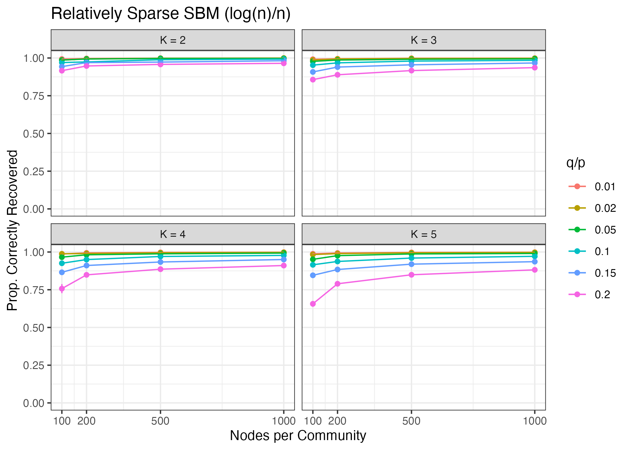
Figure 1: Proportion of nodes correctly assigned to true community from k-means clustering of the node2vec embeddings. Here we consider vary the number of nodes per community, the number of communities and the signal strength $\beta=q/p$. For each setting we consider 10 simulations, and show the mean proportion of nodes correctly recovered, with error bars indicating one standard error.

To evaluate the performance of this community detection procedure, we compute the proportion of nodes correctly classified, up to permutation of the community assignments. For each simulation setting we repeat this procedure 10 times. We show the resulting estimates in Figure 1, for the relatively sparse setting where $\rho_{n}=\log(n)/n$. For all simulation settings, the proportion of nodes assigned to the correct community by k-means clustering of the node2vec embeddings is high, particularly when the ratio of the between to within community edge probabilities, $\beta$, is small. As expected, as we increase the number of nodes in the network, a larger proportion of nodes are correctly recovered. In the supplementary material we consider other community recovery metrics, such as the widely used adjusted rand index (ARI) [17]. In each of our simulation settings we see large ARI values, increasing as the number of nodes increases.

We can similarly evaluate the performance of node2vec for data generated from a degree corrected SBM (DC-SBM). Here, to generate such networks, we modify the simulation setting used by [10]. In particular, we generate the degree correction parameters $\theta_{u}=|Z_{u}|+1-(2\pi)^{-1/2}$ where $Z_{u}\sim N(0,\sigma=0.25)$. We incorporate these degree parameters into the $\text{SBM}(n/\kappa,\kappa,p,q,\rho_{n})$ considered previously. For two nodes $u$ and $v$ in the same community, their connection probability will be $\theta_{u}\theta_{v}\rho_{n}p$ while for nodes in different communities it will be $\theta_{u}\theta_{v}\rho_{n}q$. We again learn an embedding of the nodes using a default implementation of node2vec and cluster these embedding vectors using k-means clustering. We show the corresponding results, in terms of the proportion of the nodes assigned to their correct communities under this setting in Figure 2. As expected, the degree corrections make community recovery somewhat more challenging however as we increase the number of nodes in the network, we are able to correctly recover a high proportion of nodes.

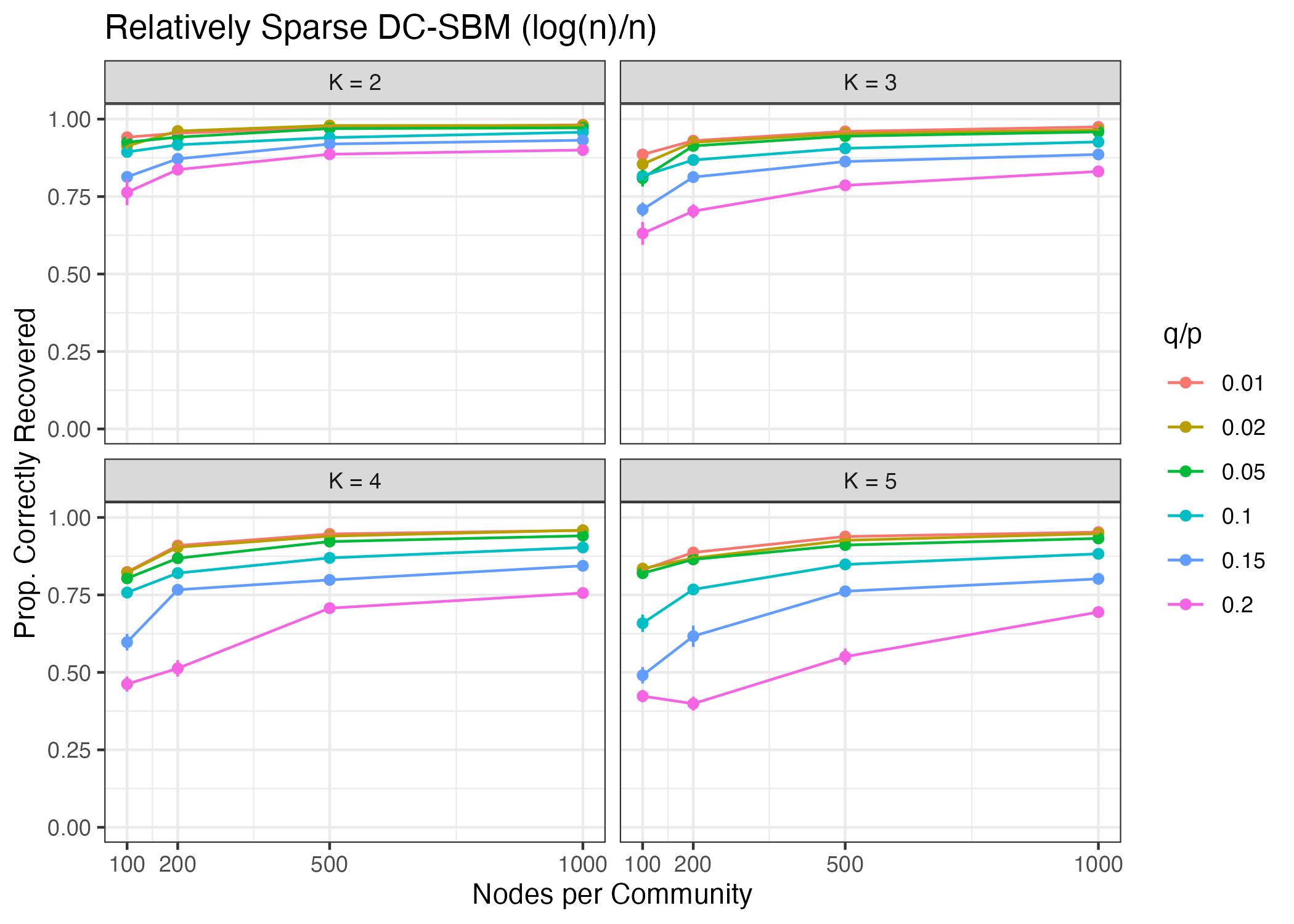
Figure 2: The proportion of nodes correctly recovered by node2vec with k-means clustering, for networks simulated from a DC-SBM. We show the mean and errorbars denoting one standard error, across 10 replications for each setting. Performance improves as $n$ increases.

We next wish to examine empirically the role of the unigram parameter $\alpha$ of Equation (7), and how this affects community detection. While the previous theoretical results require $\alpha=1$ for weak consistency of community recovery in the DC-SBM, we wish to investigate if good empirical community recovery is possible with other choices of this parameter. We consider again the DC-SBM model, where we now vary $\alpha\in\{-1,0,0.25,0.5,0.75,1\}$. For each of these settings (with the other parameters as before) we consider the proportion of nodes correctly recovered. We show this result for networks with $\kappa=2$ communities in Figure 3. These experiments indicate similar performance for the range of values of $\alpha$ considered. Further work is needed to confirm the guarantees do indeed extend to these alternative choices of $\alpha$, and we discuss this further in the Section 5 of the supplementary materials.

Figure 3: Proportion of nodes correctly recovered using node2vec and k-means clustering as we vary the negative sampling parameter in node2vec. We show the mean and errorbars denoting one standard error from 10 replications for each setting. In each case as the number of nodes increases community recovery improves, with similar performance for each choice of $\alpha$.

5 Conclusion and Future Work

In this work we consider the theoretical properties of node embeddings learned from node2vec. We show, when the network is generated from a (degree corrected) stochastic block model, that the embeddings learned from node2vec converge asymptotically to vectors depending only on their community assignment. As a result, we are able to show that K-means clustering of the embedding vectors learned from node2vec can provide weakly consistent estimates of the true community assignments of the nodes in the network. We verify these results empirically using simulated networks.

There are several important future directions which can extend this work. Our results verify that weakly consistent community recovery is possibly for a regular SBM with any choice of $\alpha$, the negative sampling hyperparameter. While we only have guarantees for a DC-SBM with this $\alpha=1$, our simulation studies indicate that a more general result is possible.

We have also not considered the task of estimating $\kappa$, the number of communities in a SBM model, using the embeddings obtained by node2vec. This has been considered for alternative approaches to community detection, ([18, 23] are some recent results) but not in the context of a general embedding of the nodes. There is also the matter of increasing the strength of our results to give strongly consistent community detection, and obtaining consistency results for other types of modern network embedding methods.

References

Supplemental Materials: Community Detection and Classification Guarantees Using Embeddings Learned by Node2Vec

The Supplementary Material consists of the proofs of the results stated within the paper, along with some extra discussions which would detract from the flow of the main paper. We also provide some additional simulation results relating to node classification, and community detection when measuring performance in terms of the ARI metric.

Appendix A Additional Notation

We give a brief recap of some of the notation introduced in the main paper, along with some more notation which is used purely within the Supplemntary Material. Throughout, we will suppose that the graph $\mathcal{G}=(\mathcal{V},\mathcal{E})$ is drawn according to the following generative model: each vertex $u\in\mathcal{V}$ have latent variables $\lambda_{u}=(c(u),\theta_{u})$ where $c(u)\in[\kappa]$ is a community assignment, and $\theta_{u}$ is a degree-heterogenity correction factor. We then suppose that the edges $a_{uv}\in\{0,1\}$ in the graph $\mathcal{G}_{n}$ on $n$ vertices arise independently with probability

$$\mathbb{P}(A_{uv}=1\,|\,\lambda_{u},\lambda_{v})=\rho_{n}\theta_{u}\theta_{v}P_{c(u),c(v)}$$ (S1)

for $u<v$, with $a_{uv}=a_{vu}$ by symmetry for $u>v$. The factor $\rho_{n}$ accounts for sparsity in the network. The above model corresponds to a degree corrected stochastic block model [19]; we highlight that the case where $\theta_{u}$ is constant across all $u\in\mathcal{V}$ corresponds to the original stochastic block model [15]. For convenience, we will write

$$W(\lambda_{u},\lambda_{v})=\theta_{u}\theta_{v}P_{c(u),c(v)}\qquad\text{ so }\qquad\mathbb{P}(A_{uv}=1\,|\,\lambda_{u},\lambda_{v})=\rho_{n}W(\lambda_{u},\lambda_{v}).$$ (S2)

We then introduce the notation

$$W(\lambda_{i},\cdot):=\mathbb{E}[W(\lambda_{i},\lambda_{j})\,|\,\lambda_{i}],\qquad\mathcal{E}_{W}(\alpha):=\mathbb{E}[W(\lambda_{i},\cdot)^{\alpha}]\text{ for }\alpha>0.$$ (S3)

Note that under the assumptions that the community assignments are drawn i.i.d from a $\mathrm{Categorical}(\pi)$ random variable, and the degree correction factors are drawn i.i.d from a distribution $\vartheta$ independently of the community assignments, we have

$$W(\lambda_{i},\cdot) =\theta_{i}\cdot\mathbb{E}[\theta]\cdot\mathbb{E}_{j\sim\mathrm{Cat}(\pi)}[P_{c(i),j}\,|\,c(i)]=\theta_{i}\cdot\mathbb{E}[\theta]\cdot\sum_{j=1}^{\kappa}\pi_{j}P_{c(i),j},$$ (S4)

$$\mathcal{E}_{W}(\alpha) =\mathbb{E}[\theta^{\alpha}]\cdot\mathbb{E}[\theta]^{\alpha}\cdot\sum_{i=1}^{\kappa}\pi_{i}\Big{(}\sum_{j=1}^{\kappa}\pi_{j}P_{i,j}\Big{)}^{\alpha}$$ (S5)

For convenience, we will write $\widetilde{P}_{c(i)}=\sum_{j=1}^{\kappa}\pi_{j}P_{c(i),j}$.

Recall that node2vec attempts to minimize the objective

$$\mathcal{L}_{n}(U,V):=\sum_{i\neq j}\Big{\{}-\mathbb{P}\big{(}(i,j)\in\mathcal{P}(\mathcal{G}_{n})\,|\,\mathcal{G}_{n}\big{)}\log(\sigma(\langle u_{i},v_{j}\rangle))-\mathbb{P}\big{(}(i,j)\in\mathcal{N}(\mathcal{G}_{n})\,|\,\mathcal{G}_{n}\big{)}\log(1-\sigma(\langle u_{i},v_{j}\rangle))\big{\}}$$ (S6)

where $U,V\in\mathbb{R}^{n\times d}$, with $u_{i},v_{j}\in\mathbb{R}^{d}$ denoting the $i$-th and $j$-th rows of $U$ and $V$ respectively, and $\sigma(x):=(1+e^{-x})^{-1}$ denoting the sigmoid function. Here $\mathcal{P}$ and $\mathcal{N}$ correspond to the positive and negative sampling schemes induced by the random walk and unigram mechanisms respectively.

Appendix B Proof of Theorems 1 and 2

B.1 Proof overview

To give an overview of the proof approach, we work by forming successive approximations to the function $\mathcal{L}_{n}(U,V)$ where we have uniform convergence of the approximation error as $n\to\infty$ over either level sets of the function considered, or the overall domain of optimization of the embedding matrices $U$ and $V$. We break these approximations up into multiple steps:

1. Lemma S1 and Proposition S2 - We begin by working with an approximation $\widehat{\mathcal{L}}_{n}(U,V)$ of $\mathcal{L}_{n}(U,V)$, where the sampling weights $\mathbb{P}\big{(}(i,j)\in\mathcal{P}(\mathcal{G}_{n})\,|\,\mathcal{G}_{n}\big{)}$ and $\mathbb{P}\big{(}(i,j)\in\mathcal{N}(\mathcal{G}_{n})\,|\,\mathcal{G}_{n}\big{)}$ are replaced by functions of the latent variables $(\lambda_{i},\lambda_{j})$ of the vertices $i$ and $j$, along with $a_{ij}$ in the case of $f_{\mathcal{P}}(\lambda_{i},\lambda_{j})$.

2. The resulting approximation $\widehat{\mathcal{L}}_{n}(U,V)$ has a dependence on the adjacency matrix of the network. We argue that this loss function converges uniformly to its average over the adjacency matrix when the vertex latent variables remain fixed; this is the contents of Theorem S3.

3. So far, the loss function only looks between interactions of $u_{i}$ and $v_{j}$ for $i\neq j$. For theoretical purposes, it is more convenient to work with a loss function where the term with $i=j$ is included. This is handled within Lemma S4.

4. Now that we have an averaged version of the loss function to work with, we are able to examine the minima of this loss function, and find that there is a unique minima (in the sense that for any pair of optima matrices $U^{*}$ and $V^{*}$, the matrix $U^{*}(V^{*})^{T}$ is unique). Moreover, in certain circumstances we can give closed forms for these minima. This is the contents of Section B.6.

5. This is then all combined together in order to give Theorems S11 and S12, which correspond to Theorems 1 and 2 of the main text.

Throughout, we also contextualize the proof by examining what it says for a SBM$(n,\kappa,p,q,\rho_{n})$ model. This corresponds to a balanced network with $pi=(\kappa^{-1},\ldots,\kappa^{-1})$.

B.2 Replacing the sampling weights

Before giving an approximation to $\mathcal{L}_{n}(U,V)$, we need to first come up with approximate forms of $\mathbb{P}\big{(}(i,j)\in\mathcal{P}(\mathcal{G}_{n})\,|\,\mathcal{G}_{n}\big{)}$ and $\mathbb{P}\big{(}(i,j)\in\mathcal{N}(\mathcal{G}_{n})\,|\,\mathcal{G}_{n}\big{)}$. The lemma below describes how we can do this.

Lemma S1.

Denote

$$f_{\mathcal{P}}(\lambda_{i},\lambda_{j}):=\frac{2k}{\rho_{n}\mathcal{E}_{W}(1)},\qquad f_{\mathcal{N}}(\lambda_{i},\lambda_{j}):=\frac{l(k+1)}{\mathcal{E}_{W}(1)\mathcal{E}_{W}(\alpha)}\big{(}W(\lambda_{i},\cdot)W(\lambda_{j},\cdot)^{\alpha}+W(\lambda_{i},\cdot)^{\alpha}W(\lambda_{j},\cdot)\big{)}.$$ (S7)

Then we have that

$$\max_{i\neq j}\Bigg{|}\frac{n^{2}\mathbb{P}\big{(}(i,j)\in\mathcal{P}(\mathcal{G}_{n})\,|\,\mathcal{G}_{n}\big{)}}{a_{ij}f_{\mathcal{P}}(\lambda_{i},\lambda_{j})}-1\Bigg{|}=O_{p}\Big{(}\Big{(}\frac{\log n}{n\rho_{n}}\Big{)}^{1/2}\Big{)},$$ (S8)

$$\max_{i\neq j}\Bigg{|}\frac{n^{2}\mathbb{P}\big{(}(i,j)\in\mathcal{N}(\mathcal{G}_{n})\,|\,\mathcal{G}_{n}\big{)}}{f_{\mathcal{N}}(\lambda_{i},\lambda_{j})}-1\Bigg{|}=O_{p}\Big{(}\Big{(}\frac{\log n}{n\rho_{n}}\Big{)}^{1/2}\Big{)}.$$ (S9)

Proof.

This is a consequence of Proposition 26 in [7]. We highlight that the statement in [7] supposes that for the negative sampling scheme, vertices for which $a_{ij}=0$ are rejected, whereas this does not happen here. Other than for the factor of $(1-a_{ij})$ in the quoted result, the proof is otherwise unchanged, which gives the statement above for $\mathbb{P}\big{(}(i,j)\in\mathcal{N}(\mathcal{G}_{n})\,|\,\mathcal{G}_{n}\big{)}$. ∎

With this, we then get the following result:

Proposition S2.

Denote

$$\widehat{\mathcal{L}}_{n}(U,V):=\frac{1}{n^{2}}\sum_{i\neq j}\Big{\{}-f_{\mathcal{P}}(\lambda_{i},\lambda_{j})a_{ij}\log(\sigma(\langle u_{i},v_{j}\rangle))-f_{\mathcal{N}}(\lambda_{i},\lambda_{j})\log(1-\sigma(\langle u_{i},v_{j}\rangle))\big{\}}$$ (S10)

and define the set

$$\Psi_{A}:=\Big{\{}U,V\in\mathbb{R}^{n\times d}\,|\,\ \mathcal{L}_{n}(U,V)\leq A\mathcal{L}_{n}(0_{n\times d},0_{n\times d})\Big{\}}\subseteq\mathbb{R}^{n\times d}\times\mathbb{R}^{n\times d}$$ (S11)

for any constant $A>1$, where $0_{n\times d}$ denotes the zero matrix in $\mathbb{R}^{n\times d}$. Then for any set $X\subseteq\mathbb{R}^{n\times d}\times\mathbb{R}^{n\times d}$ containing the pair of zero matrices $O_{n\times d}$, we have that

$$\sup_{(U,V)\in\Psi_{A}\cap X}\big{|}\mathcal{L}_{n}(U,V)-\widehat{\mathcal{L}}_{n}(U,V)\big{|}=O_{p}\Big{(}A\cdot\Big{(}\frac{\log n}{n\rho_{n}}\Big{)}^{1/2}\Big{)},$$ (S12)

$$\mathbb{P}\Big{(}\operatorname*{arg\,min}_{(U,V)\in X}\mathcal{L}_{n}(U,V)\cup\operatorname*{arg\,min}_{(U,V)\in X}\widehat{\mathcal{L}}_{n}(U,V)\subseteq\Psi_{A}\cap X\Big{)}=1-o(1).$$ (S13)

Proof.

The proof is essentially equivalent to Lemma 32 of [7] up to changes in notation, and so we do not repeat the details. ∎

Note that in practice we can choose $A$ to be any constant greater than $1$ but fixed with $n$ - e.g $A=10$, and have the result hold. We will do so going forward.

B.3 Averaging over the adjacency matrix of the graph

Following the proof outline, the next step is to argue that $\mathcal{L}_{n}(U,V)$ is close to its expectation when we average over the adjacency matrix of the graph $\mathcal{G}_{n}$. Note that we have

$$\mathbb{E}[\widehat{\mathcal{L}}_{n}(U,V)\,|\,\lambda]=\frac{1}{n^{2}}\sum_{i\neq j}\Big{\{}-f_{\mathcal{P}}(\lambda_{i},\lambda_{j})\rho_{n}W(\lambda_{u},\lambda_{v})\log(\sigma(\langle u_{i},v_{j}\rangle))-f_{\mathcal{N}}(\lambda_{i},\lambda_{j})\log(1-\sigma(\langle u_{i},v_{j}\rangle))\Big{\}}$$ (S14)

and so

$$E_{n}(U,V) :=\frac{\mathcal{E}_{W}(1)}{2k}\Big{(}\widehat{\mathcal{L}}_{n}(U,V)-\mathbb{E}[\widehat{\mathcal{L}}_{n}(U,V)\,|\,\lambda]\Big{)}$$ (S15)

$$=\frac{1}{n^{2}}\sum_{i\neq j}\Big{(}\rho_{n}^{-1}a_{ij}-W(\lambda_{i},\lambda_{j})\Big{)}\cdot(-\log\sigma(\langle u_{i},v_{j}\rangle)).$$ (S16)

Note that $\mathbb{E}[E_{n}(U,V)\,|\,\lambda]=0$, and so it therefore suffices to control $E_{n}(U,V)-\mathbb{E}[E_{n}(U,V)\,|\,\lambda]$ uniformly over embedding matrices $U,V\in\mathbb{R}^{n\times d}$. This is the contents of the next theorem.

Theorem S3.

Begin by defining the set

$$B_{2,\infty}(A_{2,\infty}):=\big{\{}U\in\mathbb{R}^{n\times d}\,:\,\|U\|_{2,\infty}\leq A_{2,\infty}\big{\}}.$$ (S17)

Then we have the bound

$$\sup_{U,V\in B_{2,\infty}(A_{2,\infty})}\big{|}E_{n}(U,V)\big{|}=O_{p}\Big{(}A_{2,\infty}^{2}\Big{(}\frac{d}{n\rho_{n}}\Big{)}^{1/2}\Big{)}.$$ (S18)

In particular, we also have that

$$\sup_{U,V\in B_{2,\infty}(A_{2,\infty})}\big{|}\widehat{\mathcal{L}}_{n}(U,V)-\mathbb{E}[\widehat{\mathcal{L}}_{n}(U,V)\,|\,\lambda]\big{|}=O_{p}\Big{(}\frac{A_{2,\infty}^{2}k}{\mathcal{E}_{W}(1)}\Big{(}\frac{d}{n\rho_{n}}\Big{)}^{1/2}\Big{)}.$$ (S19)

Proof.

Begin by noting that for any set $C\subseteq\mathbb{R}^{n\times d}\times\mathbb{R}^{n\times d}$ for which $0_{n\times d}\times 0_{n\times d}\in C$, we have that

$$\sup_{(U,V)\in C}|E_{n}(U,V)| \leq\sup_{(U,V)\in C}\big{|}E_{n}(U,V)-E_{n}(0_{n\times d},0_{n\times d})\big{|}+|E_{n}(0_{n\times d},0_{n\times d})|$$ (S20)

$$\leq\sup_{(U,V),(\tilde{U},\tilde{V})\in C}\big{|}E_{n}(U,V)-E_{n}(\tilde{U},\tilde{V})\big{|}+|E_{n}(0_{n\times d},0_{n\times d})|.$$ (S21)

We therefore need to control these two terms. We begin with the second; note that as

$$E_{n}(0_{n\times d},0_{n\times d})=\frac{1}{n^{2}}\sum_{i\neq j}\Big{(}\rho_{n}^{-1}a_{ij}-W(\lambda_{i},\lambda_{j})\Big{)}\cdot\frac{1}{n^{2}}$$ (S22)

it follows by Lemma S25 that this term is $O_{p}((n^{2}\rho_{n})^{-1/2})$. For the first term, we make use of a chaining bound. Note that if we write $T_{ij}=-\log\sigma(\langle u_{i},v_{j}\rangle)$ and $S_{ij}=-\log\sigma(\langle\tilde{u}_{i},\tilde{v}_{j}\rangle)$ for $i,j\in[n]$, then we have that

$$E_{n}(U,V)-E_{n}(\tilde{U},\tilde{V})=\frac{1}{n^{2}}\sum_{i\neq j}\Big{(}\rho_{n}^{-1}a_{ij}-W(\lambda_{i},\lambda_{j})\Big{)}\cdot(T_{ij}-S_{ij}).$$ (S23)

Because the function $x\mapsto-\log\sigma(x)$ is 1-Lipschitz, it follows that

$$\|T-S\|_{F}^{2}\leq\|UV^{T}-\tilde{U}\tilde{V}^{T}\|_{F}^{2},\qquad\|T-S\|_{\infty}\leq\|UV^{T}-\tilde{U}\tilde{V}^{T}\|_{\infty}$$ (S24)

and consequently we have that

$$\mathbb{P}\big{(}|E_{n}(U,V) -E_{n}(\tilde{U},\tilde{V})|\geq u\big{)}$$ (S25)

$$\leq 2\exp\Big{(}-\min\Big{\{}\frac{u^{2}}{128\rho_{n}^{-1}n^{-4}\|UV^{T}-\tilde{U}\tilde{V}^{T}\|_{F}^{2}},\frac{u}{16\rho_{n}^{-1}n^{-2}\|UV^{T}-\tilde{U}\tilde{V}^{T}\|_{\infty}}\Big{\}}\Big{)}$$ (S26)

as a result of Lemma S25. Now, as $U,V\in B_{F}(A_{F})\cap B_{2,\infty}(A_{2,\infty})$, by Lemma S17 if we define the metrics

$$d_{F}((U_{1},V_{1}),(U_{2},V_{2})) :=\|U_{1}-U_{2}\|_{F}+\|V_{1}-V_{2}\|_{F},$$ (S27)

$$d_{2,\infty}((U_{1},V_{1}),(U_{2},V_{2})) :=\|U_{1}-U_{2}\|_{2,\infty}+\|V_{1}-V_{2}\|_{2,\infty},$$ (S28)

then we have that

$$\mathbb{P}\big{(}| E_{n}(U,V)-E_{n}(\tilde{U},\tilde{V})|\geq u\big{)}$$ (S29)

$$\leq 2\exp\Big{(}-\min\Big{\{}\frac{u^{2}}{128\rho_{n}^{-1}n^{-4}A_{F}^{2}d_{F}((U,V),(\tilde{U},\tilde{V}))^{2}},\frac{u}{16\rho_{n}^{-1}n^{-2}A_{2,\infty}d_{2,\infty}((U,V),(\tilde{U},\tilde{V}))}\Big{\}}\Big{)}.$$ (S30)

As a result of Corollary S20, it therefore follows that

$$\sup_{(U,V),(\tilde{U},\tilde{V})\in T\times T}\big{|}E_{n}(U,V)-E_{n}(\tilde{U},\tilde{V})\big{|}=O_{p}\Big{(}A_{2,\infty}^{2}\Big{(}\frac{d}{n\rho_{n}}\Big{)}^{1/2}+A_{2,\infty}^{2}\frac{d}{n\rho_{n}}\Big{)}$$ (S31)

The desired conclusion follows by combining the bounds (S22) and (S31). ∎

B.4 Adding in a diagonal term

Currently the sum in $\mathbb{E}[\widehat{\mathcal{L}}_{n}(U,V)\,|\,\lambda]$ is defined only terms $i,j$ with $i\neq j$ - it is more convenient to work with the version where the diagonal term is added in:

$$\mathcal{R}_{n}(U,V):=\frac{1}{n^{2}}\sum_{i,j\in[n]}\Big{\{}-f_{\mathcal{P}}(\lambda_{i},\lambda_{j})\rho_{n}W(\lambda_{u},\lambda_{v})\log(\sigma(\langle u_{i},v_{j}\rangle))-f_{\mathcal{N}}(\lambda_{i},\lambda_{j})\log(1-\sigma(\langle u_{i},v_{j}\rangle))\Big{\}}.$$ (S32)

We show that this does not significantly change the size of the loss function.

Lemma S4.

With the same notation as in Theorem S3, we have that

$$\sup_{U,V\in B_{2,\infty}(A_{2,\infty})}\big{|}\mathcal{R}_{n}(U,V)-\mathbb{E}[\widehat{\mathcal{L}}_{n}(U,V)\,|\,\lambda]\big{|}=O_{p}\Big{(}\frac{1}{n}A_{2,\infty}^{2}\Big{(}\frac{2k\|W\|_{\infty}}{\mathcal{E}_{W}(1)}+\frac{2l(k+1)\|W\|_{\infty}^{2}}{\mathcal{E}_{W}(1)\mathcal{E}_{W}(\alpha)}\Big{)}\Big{)}$$ (S33)

Proof.

Begin by noting that

$$0\leq\mathcal{R}_{n}(U,V) -\mathbb{E}[\widehat{\mathcal{L}}_{n}(U,V)\,|\,\lambda]$$ (S34)

$$=\frac{1}{n^{2}}\sum_{i=1}^{n}\big{\{}-f_{\mathcal{P}}(\lambda_{i},\lambda_{j})\rho_{n}W(\lambda_{u},\lambda_{v})\log(\sigma(\langle u_{i},v_{i}\rangle))-f_{\mathcal{N}}(\lambda_{i},\lambda_{j})\log(1-\sigma(\langle u_{i},v_{i}\rangle))\big{\}}.$$

Note that we can bound

$$-\log(\sigma(\langle u_{i},v_{j}))\leq|\langle u_{i},v_{i}\rangle\leq\|u_{i}\|_{2}\|v_{i}\|_{2}$$ (S35)

and similarly $-\log(1-\sigma(\langle u_{i},v_{i}\rangle))\leq|\langle u_{i},v_{i}\rangle|\leq\|u_{i}\|_{2}\|v_{i}\|_{2}$. Moreover, we have the bounds

$$f_{\mathcal{P}}(\lambda_{i},\lambda_{j})\rho_{n}W(\lambda_{i},\lambda_{j})\leq\frac{2k\|W\|_{\infty}}{\mathcal{E}_{W}(1)},\qquad f_{\mathcal{N}}(\lambda_{i},\lambda_{j})\leq\frac{2l(k+1)\|W\|_{\infty}^{2}}{\mathcal{E}_{W}(1)\mathcal{E}_{W}(\alpha)}.$$ (S36)

As a result, because $U,V\in\mathcal{B}_{2,\infty}(A_{2,\infty})$, we end up the final bound

$$\big{|}\mathcal{R}_{n}(U,V)-\mathbb{E}[\widehat{\mathcal{L}}_{n}(U,V)\,|\,\lambda]\big{|}\leq\frac{1}{n}A_{2,\infty}^{2}\Big{(}\frac{2k\|W\|_{\infty}}{\mathcal{E}_{W}(1)}+\frac{2l(k+1)\|W\|_{\infty}^{2}}{\mathcal{E}_{W}(1)\mathcal{E}_{W}(\alpha)}\Big{)}$$ (S37)

which gives the stated result as the RHS is free of $U$ and $V$. ∎

B.5 Chaining up the loss function approximations

By chaining up the prior results, we end up with the following result:

Proposition S5.

There exists a non-empty set $\Psi_{n}$ for each $n$ such that, for any set $X\subseteq\mathbb{R}^{n\times d}\times\mathbb{R}^{n\times d}$ containing $0_{n\times d}\times 0_{n\times d}$, we have that

$$\begin{gathered}\sup_{(U,V)\in\Psi_{n}\cap B_{2,\infty}(A_{2,\infty})}\big{|}\mathcal{L}_{n}(U,V)-\mathcal{R}_{n}(U,V)\big{|}=O_{p}\Big{(}\Big{(}\frac{\log n}{n\rho_{n}}\Big{)}^{1/2}+A_{2,\infty}^{2}\Big{(}\frac{d}{n\rho_{n}}\Big{)}^{1/2}\Big{)},\\ \mathbb{P}\Big{(}\operatorname*{arg\,min}_{(U,V)\in B_{2,\infty}(A_{2,\infty})\cap X}\mathcal{L}_{n}(U,V)\cup\operatorname*{arg\,min}_{(U,V)\in B_{2,\infty}(A_{2,\infty})\cap X}\mathcal{R}_{n}(U,V)\subseteq\Psi_{A}\cap B_{2,\infty}(A_{2,\infty})\cap X\Big{)}=1-o(1).\end{gathered}$$ (S38)

The same result holds when we constrain $U=V$, but otherwise keep everything else unchanged.

B.6 Minimizers of $\mathcal{R}_{n}(U,V)$

Recall that we have earlier defined

$$\mathcal{R}_{n}(U,V):=\frac{1}{n^{2}}\sum_{i,j\in[n]}\Big{\{}-f_{\mathcal{P}}(\lambda_{i},\lambda_{j})\rho_{n}W(\lambda_{u},\lambda_{v})\log(\sigma(\langle u_{i},v_{j}\rangle))-f_{\mathcal{N}}(\lambda_{i},\lambda_{j})\log(1-\sigma(\langle u_{i},v_{j}\rangle))\Big{\}}.$$ (S39)

We now want to reason about the minima of these functions. To do so, note that the optimization domain is non-convex - firstly due to the rank constraints on the matrix $UV^{T}$, and secondly due to the fact that the loss function is invariant to any mapping $(U,V)\to(UM,VM^{-1})$ for any invertible $d\times d$ matrix $M$. To handle the second part, we consider the global minima of this function when parameterized only in term of the matrix $UV^{T}$. We will then see that the minima matrix is already low rank.

We first begin by giving some basic facts about the function $\mathcal{R}_{n}(U,V)$ when parameterized as a function of $UV^{T}$.

Lemma S6.

Define the modified function

$$\mathcal{R}_{n}(M):=\frac{1}{n^{2}}\sum_{i,j\in[n]}\Big{\{}-f_{\mathcal{P}}(\lambda_{i},\lambda_{j})\rho_{n}W(\lambda_{u},\lambda_{v})\log(\sigma(M_{ij}))-f_{\mathcal{N}}(\lambda_{i},\lambda_{j})\log(1-\sigma(M_{ij}))\Big{\}}.$$ (S40)

over all matrices $M\in\mathbb{R}^{n\times n}$. Then we have the following:

1. The function $\mathcal{R}_{n}(M)$ is strictly convex in $M$.

2. The global minimizer of $\mathcal{R}_{n}(M)$ is given by

   $$M^{*}_{ij}=\log\Big{(}\frac{f_{\mathcal{P}}(\lambda_{i},\lambda_{j})\rho_{n}W(\lambda_{i},\lambda_{j})}{f_{\mathcal{N}}(\lambda_{i},\lambda_{j})}\Big{)}$$ (S41)

   and satisfies $\nabla_{M}\mathcal{R}_{n}(M)=0$.

3. When restricted to a cone of semi-positive definite matrices $M\in\mathcal{M}_{n}^{\curlyeqsucc 0}$, there exists a unique minimizer to $\mathcal{R}_{n}(M)$ over this set, which we call $M^{\curlyeqsucc 0}$. Moreover, $M^{\curlyeqsucc 0}$ has the property that $\langle\nabla_{M}\mathcal{R}_{n}(M^{\curlyeqsucc 0}),M^{\curlyeqsucc 0}-M\rangle\leq 0$ for all $M\in\mathcal{M}_{n}^{\curlyeqsucc 0}$.

Proof.

For part a), this follows by the fact that the functions $-\log(\sigma(x))$ and $-\log(1-\sigma(x))$ are positive and strictly convex functions of $x\in\mathbb{R}$, the fact that $f_{\mathcal{P}}(\lambda_{i},\lambda_{j})\rho_{n}W(\lambda_{i},\lambda_{j})$ and $f_{\mathcal{N}}(\lambda_{i},\lambda_{j})$ are positive quantities which are bounded above (see e.g Lemma S4), and the fact that the sum of strictly convex functions is strictly convex. For part b), this follows by noting that each of the $M_{ij}^{*}$ are pointwise minima of the functions

$$r_{ij}(x)=-f_{\mathcal{P}}(\lambda_{i},\lambda_{j})\rho_{n}W(\lambda_{u},\lambda_{v})\log(\sigma(x)))-f_{\mathcal{N}}(\lambda_{i},\lambda_{j})\log(1-\sigma(x))$$ (S42)

defined over $x\in\mathbb{R}$. Indeed, note that

$$\frac{dr_{ij}}{dx}=(-1+\sigma(x))f_{\mathcal{P}}(\lambda_{i},\lambda_{j})\rho_{n}W(\lambda_{u},\lambda_{v})+\sigma(x)f_{\mathcal{N}}(\lambda_{i},\lambda_{j}),$$ (S43)

so setting this equal to zero, rearranging and making use of the equality $\sigma^{-1}(a/(a+b))=\log(a/b)$ gives the stated result. Part c) is a consequence of strong convexity, the optimization domain being convex and self dual, and the KKT conditions. ∎

To understand the form of the the global minimizer of $\mathcal{R}_{n}(M)$, by substituting in the values for $f_{\mathcal{P}}(\lambda_{i},\lambda_{j})$ and $f_{\mathcal{N}}(\lambda_{i},\lambda_{j})$ we end up with

$$M_{ij}^{*}= \log\Big{(}\frac{2P_{c(i),c(j)}\mathcal{E}_{W}(\alpha)}{(1+k^{-1})\mathbb{E}[\theta]\mathbb{E}[\theta]^{\alpha}\big{(}\theta_{j}^{\alpha-1}\widetilde{P}_{c(i)}\widetilde{P}_{c(j)}^{\alpha}+\theta_{i}^{\alpha-1}\widetilde{P}_{c(i)}^{\alpha}\widetilde{P}_{c(j)}\big{)}}\Big{)}$$ (S44)

$$= \log\Big{(}\frac{2\mathcal{E}_{W}(\alpha)}{(1+k^{-1})\mathbb{E}[\theta]\mathbb{E}[\theta]^{\alpha}}\cdot\frac{P_{c(i),c(j)}}{\widetilde{P}_{c(i)}\widetilde{P}_{c(j)}\cdot\big{(}\theta_{i}^{\alpha-1}\widetilde{P}_{c(i)}^{\alpha-1}+\theta_{j}^{\alpha-1}\widetilde{P}_{c(j)}^{\alpha-1}\big{)}}\Big{)}$$ (S45)

In particular, from the above formula we get the following lemma as a consequence:

Lemma S7.

Suppose that either i) $\theta_{i}$ is constant for all $i$, or ii) $\alpha=1$. Then if we write $\Pi_{C}\in\mathbb{R}^{n\times\kappa}$ for the matrix where $(\Pi_{C})_{il}=1[c(i)=l]$, and define the matrix

$$(\widetilde{M}^{*}_{\alpha})_{lm}=\log\Big{(}\frac{2\mathcal{E}_{W}(\alpha)}{(1+k^{-1})\mathbb{E}[\theta]\mathbb{E}[\theta]^{\alpha}}\cdot\frac{P_{lm}}{\widetilde{P}_{m}\widetilde{P}_{l}^{\alpha}+\widetilde{P}_{m}^{\alpha}\widetilde{P}_{l}}\Big{)}\;\text{ for }l,m\in[\kappa],$$ (S46)

then we have that $M^{*}=\Pi_{C}\widetilde{M}^{*}_{\alpha}\Pi_{C}^{T}$. In particular, as soon as the matrix $\Pi_{C}$ is of full rank (which occurs with asymptotic probability 1), then the rank of $M^{*}$ equals the rank of $\widetilde{M}^{*}_{\alpha}$. Moreover, as soon as $d$ is greater than or equal to the rank of $\widetilde{M}^{*}_{\alpha}$, $(U,V)$ is a minimizer of $\mathcal{R}_{n}(U,V)$ if and only if $UV^{T}=M^{*}$.

We discuss in Appendix E what happens when neither of the above conditions are satisfied. To give an example of what $M^{*}$ looks like, we write it down in the case of a $\mathrm{SBM}(n,\kappa,p,q,\rho_{n})$ model, which is frequently used to illustrate the behavior of various community detection algorithms. Such a model assumes that the community assignments $\pi_{l}=1/\kappa$ for all $l\in[\kappa]$, and that

$$P_{kl}=\begin{cases}p&\text{ if }k=l,\\ q&\text{ if }k\neq l.\end{cases}$$ (S47)

In this case, we have that

$$\widetilde{P}_{l}=\frac{p+\kappa(q-1)}{\kappa}\text{ for }l\in[\kappa],\qquad\mathcal{E}_{W}(\alpha)=\mathbb{E}[\theta]^{\alpha}\mathbb{E}[\theta^{\alpha}]\cdot\Big{(}\frac{p+(\kappa-1)q}{\kappa}\Big{)}^{\alpha}.$$ (S48)

Substituting these values into the matrix $\widetilde{M}_{\alpha}^{*}$ gives

$$(\widetilde{M}^{*}_{\alpha})_{lm}=\log\Big{(}\frac{\mathbb{E}[\theta^{\alpha}]}{\mathbb{E}[\theta](1+k^{-1})}\cdot\frac{\kappa p}{p+(\kappa-1)q}\Big{)}\delta_{lm}+\log\Big{(}\frac{\mathbb{E}[\theta^{\alpha}]}{\mathbb{E}[\theta](1+k^{-1})}\cdot\frac{\kappa q}{p+(\kappa-1)q}\Big{)}(1-\delta_{lm}).$$ (S49)

We highlight this is a matrix of the form $\alpha\delta_{lm}+\beta(1-\delta_{lm})$, and so it is straightforward to describe the spectral behavior of the matrix (see Lemma S26).

B.6.1 Minimizers in the constrained regime $U=V$

In the case where we have constrained $U=V$, it is not possible in general to write down the closed form of the minimizer of $\mathcal{R}_{n}(M)$ over $\mathcal{M}_{n}^{\curlyeqsucc 0}$. However, it is still possible to draw enough conclusions about the form of the minimizer in order to give guarantees for community detection. We begin with the proposition below.

Proposition S8.

Suppose that $\theta_{i}=1$ for all $i$. Supposing that $\widetilde{M}\in\mathbb{R}^{\kappa\times\kappa}$ is of the form $\widetilde{M}=\widetilde{U}\widetilde{U}^{T}$ for matrices $\widetilde{U}\in\mathbb{R}^{\kappa\times d}$, define the function

$$\widetilde{\mathcal{R}}_{n}(\widetilde{M})=\sum_{l,m\in[\kappa]}\hat{p}_{n}(l)\hat{p}_{n}(m)\Big{\{}-2kP_{lm}\log\sigma(\langle u_{l},u_{m}\rangle)-\{\widetilde{P}_{l}\widetilde{P}_{m}^{\alpha}+\widetilde{P}_{m}\widetilde{P}_{l}^{\alpha}\}\log(1-\sigma(\langle u_{l},u_{m}\rangle))\Big{\}}$$ (S50)

where we define $\hat{p}_{n}(l):=n^{-1}|\{i\,:\,c(i)=l\}|$ for $l\in[\kappa]$. Then $\widetilde{\mathcal{R}}_{n}(\widetilde{M})$ is strongly convex, and moreover has a unique minimizer as soon as $d\geq\kappa$.

Moreover, any minimizer of $\mathcal{R}_{n}(M)$ over matrices $M$ of the form $M=UU^{T}$ where $U\in\mathbb{R}^{n\times d}$ must take the form $M=\Pi_{C}M^{*}\Pi_{C}^{T}$ where $(\Pi_{C})_{il}=1[c(i)=l]$ where $M^{*}$ is a minimizer of $\widetilde{\mathcal{R}}_{n}(\widetilde{M})$. In particular, once $d\geq\kappa$, there is a unique minimizer to $\mathcal{R}_{n}(M)$.

Proof.

The properties of $\widetilde{\mathcal{R}}_{n}(\widetilde{M})$ are immediate by similar arguments to Lemma S6 and standard facts in convex analysis. We begin by noting that if we substitute in the values

$$\rho_{n}W(\lambda_{i},\lambda_{j})f_{\mathcal{P}}(\lambda_{i},\lambda_{j}) =\frac{2kP_{c(i),c(j)}}{\mathcal{E}_{W}(1)},$$ (S51)

$$f_{\mathcal{N}}(\lambda_{i},\lambda_{j}) =\frac{l(k+1)}{\mathcal{E}_{W}(1)\mathcal{E}_{W}(\alpha)}\big{(}\widetilde{P}_{c(i)}\widetilde{P}_{c(j)}^{\alpha}+\widetilde{P}_{c(j)}\widetilde{P}_{c(i)}^{\alpha}\big{)},$$ (S52)

for $f_{\mathcal{P}}(\lambda_{i},\lambda_{j})$ and $f_{\mathcal{N}}(\lambda_{i},\lambda_{j})$, then we can write that (recalling that $M_{ij}=\langle u_{i},u_{j}\rangle$)

$$\mathcal{R}_{n}(M) :=\frac{1}{n^{2}}\sum_{i,j\in[n]}\Big{\{}-2kP_{c(i),c(j)}\log\sigma(\langle u_{i},u_{j}\rangle)$$ (S53)

$$\qquad\qquad\qquad\qquad\qquad\qquad-\frac{l(k+1)}{\mathcal{E}_{W}(1)\mathcal{E}_{W}(\alpha)}\big{(}\widetilde{P}_{c(i)}\widetilde{P}_{c(j)}^{\alpha}+\widetilde{P}_{c(j)}\widetilde{P}_{c(i)}^{\alpha}\big{)}\log(1-\sigma(\langle u_{i},u_{j}\rangle))\Big{\}}$$ (S54)

$$:=\sum_{l,m\in[\kappa]}\hat{p}_{n}(l)\hat{p}_{n}(m)\Big{\{}-2kP_{lm}\frac{1}{|\mathcal{C}_{l}||\mathcal{C}_{m}|}\sum_{i\in\mathcal{C}_{l},j\in\mathcal{C}_{m}}\log\sigma(\langle u_{i},u_{j}\rangle)$$ (S55)

$$\qquad\qquad\qquad\qquad\qquad\qquad-\{\widetilde{P}_{c(i)}\widetilde{P}_{c(j)}^{\alpha}+\widetilde{P}_{c(j)}\widetilde{P}_{c(i)}^{\alpha}\}\frac{1}{|\mathcal{C}_{l}||\mathcal{C}_{m}|}\sum_{i\in\mathcal{C}_{l},j\in\mathcal{C}_{m}}\log(1-\sigma(\langle u_{i},u_{j}\rangle))\Big{\}}$$ (S56)

where for $l\in[\kappa]$ we define $\hat{p}_{n}(l):=n^{-1}|\{i\,:\,c(i)=l\}|$, along with the sets $\mathcal{C}_{l}=\{i\,:\,c(i)=l\}$. Now, note that as the functions $-\log(\sigma(x))$ and $-\log(1-\sigma(x))$ are strictly convex, by Jensen’s inequality we have that e.g

$$\frac{1}{|\mathcal{C}_{l}||\mathcal{C}_{m}|}\sum_{i\in\mathcal{C}_{l},j\in\mathcal{C}_{m}}-\log\sigma(\langle u_{i},u_{j}\rangle)\geq-\log\sigma\Big{(}\Big{\langle}\frac{1}{|\mathcal{C}_{l}|}\sum_{i\in\mathcal{C}_{l}}u_{i},\frac{1}{|\mathcal{C}_{m}|}\sum_{j\in\mathcal{C}_{m}}u_{j}\Big{\rangle}\Big{)}$$ (S57)

(where we also used bilinearity of the inner product) where equality holds above if and only if the $u_{i}$ are constant are across all indices $i$. In particular, any minimizer of $\mathcal{R}_{n}(M)$ must have the $u_{i}$ constant across $i\in\mathcal{C}_{l}$ for each $l\in[\kappa]$, which defines the function $\tilde{\mathcal{R}}_{n}(\widetilde{M})$. This gives the claimed statement. ∎

In certain cases, we are able to give a closed form to the minimizer. We illustrate this for the case of the SBM$(n,\kappa,p,q,\rho_{n})$ model.

Proposition S9.

Let $\widetilde{M}^{*}$ be the unique minimizer of $\tilde{\mathcal{R}}_{n}(\widetilde{M})$ as introduced in Proposition S8. In the case of a SBM$(\kappa,p,q,\rho_{n})$ model, we have that $\kappa^{-2}\|\widetilde{M}^{*}-M^{*}\|_{1}=O_{p}((\kappa\log\kappa/n)^{1/4})$, where $M^{*}$ is of the form

$$(M^{*})_{ij}=\alpha^{*}\delta_{ij}-\frac{\alpha^{*}}{\kappa-1}(1-\delta_{ij})$$ (S58)

for some $\alpha^{*}=\alpha^{*}(p,q)\geq 0$. Moreover, $\alpha^{*}>0$ iff $p>q$.

Proof.

We begin by arguing that the objective function $\widetilde{\mathcal{R}}_{n}(\widetilde{M})$ converges uniformly to the objective

$$\bar{\mathcal{R}}_{n}(\widetilde{M}):=\frac{1}{\kappa^{2}}\sum_{l,m\in[\kappa]}\Big{\{}-2kP_{lm}\log\sigma(\langle u_{l},u_{m}\rangle)-\{\widetilde{P}_{m}\widetilde{P}_{l}^{\alpha}+\widetilde{P}_{l}\widetilde{P}_{m}^{\alpha}\}\log(1-\sigma(\langle u_{l},u_{m}\rangle))\Big{\}}$$ (S59)

over a set containing the minimizers of both functions. Note that this function is also strictly convex, and has a unique minimizer as soon as $d\geq\kappa$. To do so, we highlight that as we have that

$$\max_{k\neq l}\Big{|}\frac{\hat{p}_{n}(l)\hat{p}_{n}(k)-\kappa^{-2}}{\kappa^{-2}}\Big{|}=O_{p}\Big{(}\Big{(}\frac{\kappa\log\kappa}{n}\Big{)}^{1/2}\Big{)}$$ (S60)

by standard concentration results for Binomial random variables (e.g Proposition 47 of [7]), it follows that

$$\big{|}\bar{\mathcal{R}}_{n}(\widetilde{M})-\widetilde{\mathcal{R}}_{n}(\widetilde{M})\big{|}\leq\bar{\mathcal{R}}_{n}(\widetilde{M})\cdot O_{p}\Big{(}\Big{(}\frac{\kappa\log\kappa}{n}\Big{)}^{1/2}\Big{)}.$$ (S61)

Consequently, $\widetilde{\mathcal{R}}_{n}(\widetilde{M})$ converges to $\bar{\mathcal{R}}_{n}(\widetilde{M})$ uniformly over any level set of $\bar{\mathcal{R}}_{n}(\widetilde{M})$, which necessarily contains the minima of $\bar{\mathcal{R}}_{n}(\widetilde{M})$. If one does so over the set (for example)

$$A=\{\widetilde{M}\,:\,\bar{\mathcal{R}}_{n}(\widetilde{M})\leq 10\bar{\mathcal{R}}_{n}(0)\}$$ (S62)

(for example), then as $\bar{\mathcal{R}}_{n}(0)$ is constant across $n$, we have uniform convergence of (S61) over the set $A$ at a rate of $O_{p}\big{(}(\log\kappa/np)^{1/2}\big{)}$. This argument can be reversed, which therefore ensures uniform convergence (over the same set) which contains the minimizers (with the minimizer of $\tilde{\mathcal{R}}_{n}(M)$ being contained within this set with asymptotic probability $1$) at a rate of $O_{p}\big{(}(\kappa\log\kappa/n)^{1/2}\big{)}$.

With this, we note that an application of Lemma S28 gives that for any matrices $\widetilde{M}_{1}$ and $\widetilde{M}_{2}$ we have that

$$\bar{\mathcal{R}}_{n}(\widetilde{M}_{1}) \geq\bar{\mathcal{R}}_{n}(\widetilde{M}_{2})+\langle\Delta\bar{\mathcal{R}}_{n}(\widetilde{M}_{2}),\widetilde{M}_{1}-\widetilde{M}_{2}\rangle$$ (S63)

$$\qquad+\frac{C}{\kappa^{2}}\sum_{i,j\in[\kappa]}\min\{|(\widetilde{M}_{2})_{ij}-(\widetilde{M}_{1})_{ij}|^{2},2|(\widetilde{M}_{2})_{ij}-(\widetilde{M}_{1})_{ij}|\}.$$ (S64)

where to save on notation, we define

$$C:=\frac{1}{4}e^{-\|\widetilde{M}_{2}\|_{\infty}}\min_{l,m}\{2kP_{lm},\widetilde{P}_{m}\widetilde{P}_{l}^{\alpha}\}.$$ (S65)

In particular, if $\widetilde{M}_{2}=\bar{M}^{*}$ is an optimum of $\bar{\mathcal{R}}_{n}(\widetilde{M})$, then by the KKT conditions (similarly as in Lemma S6) we have that

$$\bar{\mathcal{R}}_{n}(\widetilde{M}_{1})-\bar{\mathcal{R}}_{n}(\bar{M}^{*})\geq\frac{C}{\kappa^{2}}\sum_{i,j\in[\kappa]}\min\{|(\bar{M}^{*})_{ij}-(\widetilde{M}_{1})_{ij}|^{2},2|(\bar{M}^{*})_{ij}-(\widetilde{M}_{1})_{ij}|\}.$$ (S66)

In particular, if we then let $\widetilde{M}^{*}$ be any minimizer of $\widetilde{\mathcal{R}}_{n}(\widetilde{M})$, then we have that

$$\frac{C}{\kappa^{2}}\sum_{i,j\in[\kappa]} \min\{|(\bar{M}^{*})_{ij}-(\widetilde{M}_{1})_{ij}|^{2},2|(\bar{M}^{*})_{ij}-(\widetilde{M}_{1})_{ij}|\}$$ (S67)

$$\leq\bar{\mathcal{R}}_{n}(\widetilde{M}_{1})-\bar{\mathcal{R}}_{n}(\bar{M}^{*})\leq\bar{\mathcal{R}}_{n}(\widetilde{M}_{1})-\tilde{\mathcal{R}}_{n}(\bar{M}^{*})+\tilde{\mathcal{R}}_{n}(\widetilde{M}^{*})-\bar{\mathcal{R}}_{n}(\bar{M}^{*})$$ (S68)

$$\leq 2\sup_{M\in A}\big{|}\tilde{\mathcal{R}}_{n}(M)-\bar{\mathcal{R}}_{n}(M)\big{|}$$ (S69)

on an event of asymptotic probability $1$. Consequently, it follows by Lemma S29 that

$$\frac{1}{\kappa^{2}}\|\bar{M}^{*}-\widetilde{M}^{*}\|_{1}=O_{p}\big{(}(\kappa\log\kappa/n)^{1/4}\big{)}.$$ (S70)

We now need to find the minimizing positive semi-definite matrix which optimizes $\bar{\mathcal{R}}_{n}(\widetilde{M})$. To do so, we will argue that one can find $\alpha$ for which

$$\widehat{M}_{ij}=\alpha\delta_{ij}-\frac{\alpha}{\kappa-1}(1-\delta_{ij}),\quad\nabla\bar{\mathcal{R}}_{n}(\widehat{M})=C1_{\kappa}1_{\kappa}^{T},\quad 1_{\kappa}=(1,\cdots,1)^{T}$$

for some positive constant $C$, as then the KKT conditions for the constrained optimization problem will hold. Indeed, for any positive definite matrix $M$, as by definition of $\widehat{M}$ we have that $\langle\nabla\bar{\mathcal{R}}_{n}(\widehat{M}),\widehat{M}\rangle=0$ as all of the eigenvectors of $\widehat{M}$ are orthogonal to the unit vector $1_{\kappa}$ (Lemma S26). It consequently follows that as $\nabla\bar{\mathcal{R}}_{n}(\widehat{M})$ is itself positive definite, we get that $\langle-\nabla\bar{\mathcal{R}}_{n}(\widehat{M}),\widehat{M}-M\rangle=\langle\nabla\bar{\mathcal{R}}_{n}(\widehat{M}),M\rangle\geq 0$. We now need to verify the existence of a constant $\alpha$ for which this condition holds. We note that as $\widehat{M}_{ij}$ is constant across $i=j$, and also constant across $i\neq j$, to verify the condition that $\nabla\bar{\mathcal{R}}_{n}(\widehat{M})$ is proportional to $1_{\kappa}1_{\kappa}^{T}$, it suffices to check whether the on and off diagonal terms of $\nabla\bar{\mathcal{R}}_{n}(\widehat{M})$ are equal to each other. This gives the equation

$$\sigma(\alpha)\cdot\Big{(}kp +l(k+1)\frac{p+(\kappa-1)q}{\kappa}\Big{)}$$

$$=k(p-q)+\sigma(-\alpha/(\kappa-1))\Big{(}kq+l(k+1)\frac{p+(\kappa-1)q}{\kappa}\Big{)}$$

By applying Lemma S27, this has a singular positive solution in $\alpha$ if and only if $k(p-q)\geq k(p-q)/2$, which holds iff $p\geq q$. In the case where $p<q$, it follows that the solution has $\alpha=0$. ∎

B.7 Strong convexity properties of the minima matrix

Proposition S10.

Define the modified function

$$\mathcal{R}_{n}(M):=\frac{1}{n^{2}}\sum_{i,j\in[n]}\Big{\{}-f_{\mathcal{P}}(\lambda_{i},\lambda_{j})\rho_{n}W(\lambda_{u},\lambda_{v})\log(\sigma(M_{ij}))-f_{\mathcal{N}}(\lambda_{i},\lambda_{j})\log(1-\sigma(M_{ij}))\Big{\}}.$$ (S71)

over all matrices $M\in\mathbb{R}^{n\times n}$. Then we have for any matrices $M_{1},M_{2}\in\mathbb{R}^{n\times n}$ with $\|M_{1}\|_{\infty},\|M_{2}\|_{\infty}\leq A_{\infty}$ that

$$\mathcal{R}_{n}(M_{1})\geq\mathcal{R}_{n}(M_{2})+\langle\nabla\mathcal{R}_{n}(M_{2}),M_{1}-M_{2}\rangle+\frac{\widetilde{C}e^{-A_{\infty}}}{2}\cdot\frac{1}{n^{2}}\|M_{1}-M_{2}\|_{F}^{2}$$ (S72)

where $\widetilde{C}=\min_{l,m}\{2kP_{l,m},\tilde{P}_{l}^{\alpha}\tilde{P}_{m}\}$. Moreover,

1. If $\mathcal{R}_{n}(M)$ is constrained over a set $\mathcal{X}=\{M=UV^{T}\,:\,U,V\in\mathbb{R}^{n\times d},\|M\|_{\infty}\leq A_{\infty}\}$, and there exists $M^{*}$ in $\mathcal{X}$ such that $\nabla\mathcal{R}_{n}(M^{*})=0$, then we have that

   $$\frac{1}{n^{2}}\|M^{*}-M\|_{F}^{2}\leq C(k,l,\alpha,P,\pi,A_{\infty})\cdot\big{(}\mathcal{R}_{n}(M)-\mathcal{R}_{n}(M^{*})\big{)}\text{ for all }M\in\mathcal{X}.$$ (S73)

2. If $\mathcal{R}_{n}(M)$ is constrained over a set $\mathcal{X}^{\geq 0}=\{M=UU^{T}\,:\,U\in\mathbb{R}^{n\times d},\|M\|_{\infty}\leq A_{\infty}$ }, and there exists $M^{*}$ in $\mathcal{X}^{\geq 0}$ such that $\langle\nabla\mathcal{R}_{n}(M^{*}),M-M^{*}\rangle\geq 0$ for all $M\in\mathcal{X}^{\geq 0}$, then we get the same inequality as in part i) above.

Proof.

The first inequality follows by an application of Lemma S28, with the second and third parts following by applying the conditions stated and rearranging. ∎

B.8 Convergence of the gram matrices of the embeddings

By combining together Proposition S10 and Proposition S5 we end up with the following result:

Theorem S11.

Suppose that the conditions of Lemma S7 hold. (In particular, recall that $d\geq\kappa$.) Then there exist constants $A_{\infty}$ and $A_{2,\infty}$ (depending on the parameters of the model and sampling scheme) and a matrix $M^{*}\in\mathbb{R}^{\kappa\times\kappa}$ (also depending on the parameters of the model and the sampling scheme) such that for any minimizer $(U^{*},V^{*})$ of $\mathcal{L}(U,V)$ over the set

$$X=\{(U,V)\,:\,\|U\|_{\infty},\|V\|_{\infty}\leq A_{\infty},\|U\|_{2,\infty},\|V\|_{2,\infty}\leq A_{2,\infty}\},$$ (S74)

we have that

$$\frac{1}{n^{2}}\sum_{i,j\in[n]}\big{(}\langle u_{i}^{*},v_{j}^{*}\rangle-M^{*}_{c(i),c(j)}\big{)}^{2}=C(k,l,\alpha,P,\pi,A_{\infty},A_{2,\infty})\cdot O_{p}\Big{(}\Big{(}\frac{\max\{\log n,d\}}{n\rho_{n}}\Big{)}^{1/2}\Big{)}$$ (S75)

for some constant $C(k,l,\alpha,P,\pi,A_{\infty},A_{2,\infty})>0$. In the case where we constrain $U=V$, the same result holds provided the conditions of Proposition S8 hold.

Proof.

We note that by Lemma S7, there exists a minimizer $\widetilde{M}^{*}$ for $\mathcal{R}_{n}(M)$ of the form $\widetilde{M}^{*}=\Pi M^{*}\Pi^{T}$ for a matrix $M^{*}\in\mathbb{R}^{\kappa\times\kappa}$. We can then take $A_{\infty}$ and $A_{2,\infty}$ as $2\|M^{*}\|_{\infty}$ and $2\|M^{*}\|_{2,\infty}$. We highlight that we can do this even when $d>\kappa$, as we can embed $M^{*}$ into the block diagonal matrix $\mathrm{diag}(M^{*},O_{d-\kappa,d-\kappa})$, which preserves both the norms above. Lemma S6 and Proposition S10 then guarantee that

$$\frac{1}{n^{2}}\|U^{*}(V^{*})^{T}-\widetilde{M}^{*}\|_{F}^{2}\leq\tilde{C}\cdot\big{(}\mathcal{R}_{n}(UV^{T})-\mathcal{R}_{n}(\widetilde{M}^{*})\big{)}$$ (S76)

where we write $\tilde{C}:=C(k,l,\alpha,P,\pi,A_{\infty},A_{2,\infty})$. As $\mathcal{X}$ is a subset of $\mathcal{B}_{2,\infty}(A_{2,\infty})$, and $(U^{*},V^{*})$ is a minimizer of $\mathcal{L}(U,V)$, we end up getting that

$$\big{(}\mathcal{R}_{n}(UV^{T}) -\mathcal{R}_{n}(\widetilde{M}^{*})\big{)}$$ (S77)

$$\leq\mathcal{R}_{n}(UV^{T})-\mathcal{L}_{n}(U^{*},V^{*})+\mathcal{L}_{n}(M^{*})-\mathcal{R}_{n}(\widetilde{M}^{*})\leq 2\sup_{(U,V)\in X}\big{|}\mathcal{R}_{n}(U,V)-\mathcal{L}_{n}(U,V)\big{|}$$ (S78)

from which we can apply Proposition S5 to then give the claimed result. ∎

We give some brief intuition as to the size of the constants involved here, to understand any potential hidden dependencies involved in them. Of greatest concern are the constants $A_{\infty}$ and $A_{2,\infty}$ (as the remaining constants are explicit throughout the proof, and depend only on the hyperparameters of the sampling schema and the model in a polynomial fashion). Note that in the case where $k$ is large and we have a SBM$(\kappa,p,q)$ model, from the discussion after Lemma S7, the minimizing matrix $M^{*}$ takes the form

$$(M^{*})_{lm}\approx\log\Big{(}\frac{\kappa p}{p+(\kappa-1)q}\Big{)}\delta_{lm}+\log\Big{(}\frac{\kappa q}{p+(\kappa-1)q}\Big{)}(1-\delta_{lm}).$$ (S79)

Supposing for simplicity that $p>q$, it follows that we can take can take $A_{\infty}$ to be of the order $O(\log(p/q))$ when $\kappa$ is large. In the rate from Proposition S10, this gives a rate of $O(p/q)$ from the $e^{A_{\infty}}$ factor; note that the dependence on the parameters of the models here are not unreasonable. As for $A_{2,\infty}$, we first highlight the fact that

$$(\kappa-1)\log\Big{(}\frac{\kappa q}{p+(\kappa-1)q}\Big{)}\to\frac{p-q}{q}\text{ as }\kappa\to\infty.$$ (S80)

By Lemma S26 we can therefore take $A_{2,\infty}$ to be a scalar multiple of $|\log(p/q)|^{1/2}$, avoiding any implicit dependence on $\kappa$ or the embedding dimension $d$.

B.9 Convergence of the embedding vectors

We can then get results guaranteeing the convergence of the individual embedding vectors (rather than their gram matrix) up to rotations, as stated by the following theorem.

Theorem S12.

Suppose that the conclusion of Theorem S11 holds, and further suppose that $d$ equals the rank of the matrix $M^{*}$. Then there exists a matrix $\tilde{U}^{*}\in\mathbb{R}^{\kappa\times d}$ such that

$$\min_{Q\in O(d)}\frac{1}{n}\sum_{i=1}^{n}\|u_{i}^{*}-\tilde{u}_{c(i)}^{*}Q\|_{2}^{2}=C(k,l,\alpha,P,\pi,A_{\infty},A_{2,\infty})\cdot O_{p}\Big{(}\Big{(}\frac{\max\{\log n,d\}}{n\rho_{n}}\Big{)}^{1/2}$$ (S81)

Proof.

We handle the cases where $U\neq V$ and $U=V$ separately. For the case where $U\neq V$, we note that without loss of generality we can suppose that $UU^{T}=VV^{T}$, in which case we can apply Lemma S21 and Theorem S11 to give the stated result. To do so, we note that by Lemma S23 we have that $n^{-1}\sigma_{d}(\Pi M^{*}\Pi^{T})\geq c\sigma_{d}(M^{*})$ for some constant $c$ with asymptotic probability $1$, as a result of the fact that $n_{k}(\Pi)\geq 1/2n\pi_{k}$ with asymptotic probability $1$ uniformly across all communities $k\in[\kappa]$. As moreover we have that $n^{-1}\|UV^{T}-\Pi M^{*}\Pi^{T}\|_{\text{op}}\leq n^{-1}\|UV^{T}-\Pi M^{*}\Pi^{T}\|_{F}=o_{p}(1)$, the condition that $\|UV^{T}-\Pi M^{*}\Pi^{T}\|_{\text{op}}\leq 1/2\sigma_{d}(\Pi M^{*}\Pi^{T})$ holds with asymptotic probability 1, we have verified the conditions in Lemma S21, giving the desired result. In the case where we constrain $U=V$, the same argument holds, except we no longer need to verify the condition that $\|UU^{*}-M^{*}\|_{\text{op}}$ is sufficiently small, and so we have concluded in this case also. ∎

In the case of a SBM$(n,\kappa,p,q,\rho_{n})$ model it is actually able to give closed form expressions for the embedding vectors which are converged to by factorizing the minima matrix $M^{*}$ in the way described by the above proof. These details are given in Lemma S26.

Appendix C Proof of Theorem 3, Corollary 4 and Lemma 5

C.1 Guarantees for community detection

We begin with a discussion of how we can get guarantees for community detection via approximate k-means clustering method, using the convergence criteria for embeddings we have derived already. To do so, suppose we have a matrix $U\in\mathbb{R}^{n\times d}$ corresponding of $n$ columns of $d$-dimensional vectors. Defining the set

$$M_{n,K}:=\{\Pi\in\{0,1\}^{n\times K}\,:\,\text{each row of $\Pi$ has exactly $K-1$ zero entries}\},$$ (S82)

we seek to find a factorization $U\approx\Pi X$ for matrices $\Pi\in M_{n,K}$ and $X\in\mathbb{R}^{K\times d}$. To do so, we minimize the objective

$$\mathcal{L}_{k}(\Pi,X)=\frac{1}{n}\|U-\Pi X\|_{F}^{2}$$ (S83)

In practice, this minimization problem is NP-hard [4], but we can find $(1+\epsilon)$-approximate solutions in polynomial time [21]. As a result, we consider any minimizers $\hat{\Pi}$ and $\hat{X}$ such that

$$\mathcal{L}_{k}(\hat{\Pi},\hat{X})\leq(1+\epsilon)\min_{\Pi,X}\mathcal{L}_{k}(\Pi,X).$$ (S84)

We want to examine the behavior of k-means clustering on the matrix $U$, when it is close to a matrix $U^{*}$ which has an exact factorization $U^{*}=\Pi^{*}X^{*}$ for some matrices $\Pi^{*}\in M_{n,K}$ and $X^{*}\in\mathbb{R}^{K\times d}$. We introduce the notation

$$G_{k}(\Pi):=\{i\in[n]:\Pi_{ik}=1\},\qquad n_{k}(\Pi):=|G_{k}(\pi)|$$ (S85)

for the columns of $U$ which are assigned as closest to the $k$-th column of $X$ as according to the matrix $\Pi$.

We make use of the following theorem from [27], which we restate for ease of use.

Proposition S13 (Lemma 5.3 of [27]).

Let $(\hat{\Pi},\hat{X})$ be any $(1+\epsilon)$-approximate minimizer to the k-means problem given a matrix $U\in\mathbb{R}^{n\times d}$. Suppose that $U^{*}=\Pi^{*}X^{*}$ for some matrices $\Pi^{*}\in M_{n,\kappa}$ and $X^{*}\in\mathbb{R}^{\kappa\times d}$. Fix any $\delta_{k}\leq\min_{l\neq k}\|X^{*}_{l\cdot}-X^{*}_{k\cdot}\|_{2}$, and suppose that the condition

$$(16+8\epsilon)\|U-U^{*}\|_{F}^{2}/\delta_{k}^{2}<n_{k}(\Pi^{*})\text{ for all }k\in[\kappa]$$ (S86)

holds. Then there exist subsets $S_{k}\subseteq G_{k}(\Pi^{*})$ and a permutation matrix $\sigma\in\mathbb{R}^{\kappa\times\kappa}$ such that the following holds:

1. For $G=\bigcup_{k}(G_{k}(\Pi^{*})\setminus S_{k})$, we have that $(\Pi^{*})_{G\cdot}=\sigma\Pi_{G\cdot}$. In words, outside of the sets $S_{k}$ we recover the assignments given by $\Pi^{*}$ up to a re-labelling of the clusters.

2. The inequality $\sum_{k=1}^{\kappa}|S_{k}|\delta_{k}^{2}\leq(16+8\epsilon)\|U-U^{*}\|_{F}^{2}$ holds.

In particular, we can then apply this to our consistency results with the embeddings learned by node2vec. Recall that we are interested in the following metrics measuring recovery of communities by any given procedure:

$$L(c,\hat{c}) :=\min_{\sigma\in\mathrm{Sym}(\kappa)}\frac{1}{n}\sum_{i=1}^{n}1[\hat{c}(i)\neq\sigma(c(i))],$$ (S87)

$$\widetilde{L}(c,\hat{c}) :=\max_{k\in[\kappa]}\min_{\sigma\in\mathrm{Sym}(\kappa)}\frac{1}{|\mathcal{C}_{k}|}\sum_{i\in\mathcal{C}_{k}}1[\hat{c}(i)\neq\sigma(k)].$$ (S88)

These measure the overall misclassification rate and worst-case class misclassification rate respectively.

Corollary S14.

Suppose that we have embedding vectors $\omega_{i}\in\mathbb{R}^{d}$ for $i\in[n]$ such that

$$\min_{Q\in O(d)}\frac{1}{n}\sum_{i=1}^{n}\|\omega_{i}-\eta_{C(i)}Q\|_{2}^{2}=O_{p}(r_{n})$$ (S89)

for some rate function $r_{n}\to 0$ as $n\to\infty$ and vectors $\eta_{l}\in\mathbb{R}^{d}$ for $l\in[\kappa]$. Moreover suppose that $\delta:=\min_{l\neq k}\|\eta_{l}-\eta_{k}\|_{2}>0$. Then if $\hat{c}(i)$ are the community assignments produced by applying a $(1+\epsilon)$-approximate k-means clustering to the matrix whose columns are the $\omega_{i}$, we have that $L(c,\hat{c})=O_{p}(\delta^{-2}r_{n})$ and $\widetilde{L}(c,\hat{c})=O_{p}(\delta^{-2}r_{n})$.

Proof.

We apply Proposition S13 with $\Pi^{*}$ corresponding to the matrix of community assignments according to $c(\cdot)$, and $X^{*}$ the matrix whose columns are the $Q\eta_{l}$ for $l\in[\kappa]$ where $Q\in O(d)$ attains the minimizer in (S89). Letting $U$ be the matrix whose columns are the $\omega_{i}$ and taking $\delta_{k}=\delta$, the condition (S86) to verify becomes

$$\frac{16+8\epsilon}{\delta^{2}}\frac{1}{n}\sum_{i=1}^{n}\|\omega_{i}-Q\eta_{c(i)}\|_{2}^{2}<\frac{|\mathcal{C}_{k}|}{n}\text{ for all }k\in[\kappa].$$ (S90)

As $r_{n}\to 0$ and $|\mathcal{C}_{l}|/n>c>0$ for some constant $c$ uniformly across vertices $l\in[\kappa]$ with asymptotic probability $1$ (as a result of the community generation mechanism, the communities are balanced), the above event will be satisfied with asymptotic probability 1. The desired conclusion follows by making use of the inequalities

$$L(c,\hat{c})\leq\frac{1}{n}\sum_{k\in[\kappa]}|S_{k}|,\qquad\widetilde{L}(c,\hat{c})\leq\max_{k\in[\kappa]}\frac{1}{|\mathcal{C}_{k}|}|S_{k}|\leq\Big{(}\max_{k\in[\kappa]}\frac{n}{|\mathcal{C}_{k}|}\Big{)}\cdot\frac{1}{n}\sum_{l\in[\kappa]}|S_{l}|$$ (S91)

which hold by the first consequence in Proposition S13, and then applying the bound

$$\frac{1}{n}\sum_{k\in[\kappa]}|S_{k}|\leq\frac{16+8\epsilon}{\delta^{2}}\cdot\frac{1}{n}\sum_{i=1}^{n}\|\omega_{i}-Q\eta_{c(i)}\|_{2}^{2}.\qed$$ (S92)

We note that in order to apply this theorem, we require the further separation criterion of $\delta>0$. As a result of Lemma S26, we can guarantee this for the SBM$(\kappa,p,q,\rho_{n})$ model when either a) node2vec is trained in the unconstrained setting, or b) we are in the constrained setting with $p>q$. As we know that the embedding vectors converge to the zero vector on average when we are in the constrained setting with $p\leq q$, as a result we know that community detection is possible in the constrained setting iff $p>q$, which gives Corollary 4 of the main paper.

C.2 Guarantees for node classification and link prediction

We now discuss what guarantees we can make when using the embedding vectors for classification. In this section, we suppose that we have a guarantee

$$\frac{1}{n}\min_{Q\in O(d)}\sum_{i=1}^{n}\|u_{i}-\eta_{C(i)}Q\|_{2}^{2}\leq C(\tau)r_{n}\qquad\text{ holds with probability }\geq 1-\tau$$ (S93)

for some constant $C(\tau)$ and rate function $r_{n}\to 0$ as $n\to\infty$. This is the same as saying that the LHS is $O_{p}(r_{n})$ - it will happen to be more convenient to use this formulation. We also suppose that there exists a positive constant $\delta>0$ for which

$$\delta\leq\min_{k\neq l}\|\eta_{k}-\eta_{l}\|_{2}.$$ (S94)

We begin with a lemma which discusses the underlying geometry when we take a small sample of the embedding vectors.

Lemma S15.

Suppose we sample $K$ embeddings from the set $(u_{i})_{i\in[n]}$, which we denote as $u_{i_{1}},\ldots,u_{i_{K}}$. Define the sets

$$S_{l}=\{i\in\mathcal{C}_{l}\,:\,\|u_{i}-\eta_{C(i)}\|_{2}<\delta/4\}.$$ (S95)

Then there exists $n_{0}(K,\delta,\tau^{\prime})$ such that if $n\geq n_{0}$, with probability $1-\tau^{\prime}$ we have that $u_{i_{j}}\in S_{c(i_{j})}$ for all $j\in[K]$.

Proof.

Without loss of generality, we will suppose that $Q=I$. For each $l\in[\kappa]$, define the sets $S_{l}=\{i\in\mathcal{C}_{l}\,:\,\|u_{i}-\eta_{l}\|_{2}\leq\delta/4\}$. Then by the condition (S93), by Markov’s inequality we know that with probability $1-\tau$ we have that

$$\frac{1}{n}\sum_{l\in[\kappa]}|\mathcal{C}_{l}\setminus S_{l}|\leq 4\delta^{-2}C(\tau/2)r_{n}.$$ (S96)

We now suppose that we sample $K$ embeddings uniformly at random; for convenience, we suppose that they are done so with replacement. Then the probability that all of the embeddings are outside the set $\bigcup_{l}(\mathcal{C}_{l}\setminus S_{l})$ is given by $(1-\frac{1}{n}\sum_{l}|\mathcal{C}_{l}\setminus S_{l}|)^{K}\geq 1-\frac{K}{n}\sum_{l}|\mathcal{C}_{l}\setminus S_{l}|$. In particular, this means with probability no less than $1-\tau-4K\delta^{-1}C(\tau)r_{n}$, if we sample $K$ embeddings with indices $i_{1},\ldots,i_{K}$ at random from the set of $n$ embeddings, they lie within the sets $S_{C(i_{1})},\ldots,S_{C(i_{K})}$ respectively. The desired result then follows by noting that we take $\tau=\tau^{\prime}/2$, and choose $n$ such that $4\delta^{-2}C(\tau/2)r_{n}<\tau^{\prime}/2$. ∎

To understand how this lemma can give insights into the downstream use of embeddings, suppose that we have access to an oracle which provides the community assignments of a vertex when requested, but otherwise the community assignments are unseen.

We note that in practice, only a small number of labels are needed to be provided to embedding vectors in order to achieve good classification results (see e.g the experiments in [12, 43]). As a result, we can imagine keeping $K$ fixed in the regime where $n$ is large. Moreover, the constant $\delta$ simply reflects the underlying geometry of the learned embeddings, and $\tau^{\prime}$ is a tolerance we can choose such that the stated result is very likely to hold (by e.g choosing $\tau^{\prime}=10^{-2}$ or $10^{-3}$). As a consequence, the above lemma tells us with high probability, we can

1. learn a classifier which is able to distinguish between the sets $S_{l}$ given use of the sampled embeddings $u_{i_{1}},\ldots,u_{i_{K}}$ and the labels $c(i_{1}),\ldots,c(i_{K})$, provided the classifier is flexible enough to separate $\kappa$ disjoint convex sets; and

2. as a consequence of (S96), this classifier will correctly classify a large proportion of vertices within the correct sets $S_{l}$.

The same argument applies if instead we have classes assigned to embedding vectors which form a coarser partitioning of the underlying community assignments. The importance of the above result is that in order to understand the behavior of embedding methods for classification, it suffices to understand which geometries particular classifiers are able to separate - for example, when the number of classes equals $2$, this reduces down to the classic concept of linear separability, in which case a logistic classifier would suffice.

We end with a discussion as to the task of link prediction, which asks to predict whether two vertices are connected or not given a partial observation of the network. To do so, we suppose that from the observed network, we delete half of the edges in the network, and then train node2vec on the resulting network. Note that the node2vec mechanism only makes explicit use of known edges within the network. This corresponds to training the node2vec model on the data with sparsity factor $\rho_{n}\to\rho_{n}/2$; in particular, this leaves the underlying asymptotic representations unchanged and slows the rate of convergence by a factor of 2. With this, a link prediction classifier is formed by the following process:

1. Take a set of edges $J\subseteq\{(i,j)\,:\,a_{ij}=1\}$ for which the node2vec algorithm was not trained on, and a set of non-edges $\tilde{J}\subseteq\{(i,j)\,:\,a_{ij}=0\}$. As in practice networks are sparse, these sets are not sampled randomly from the network, but are assumed to be sampled in a balanced fashion so that the sets $J$ and $\tilde{J}$ are roughly balanced in size. One way of doing so is to pick a number of edges in advance, say $E$, and then sample $E$ elements from the set of edges and non-edges in order to form $J$ and $\tilde{J}$ respectively.

2. Form edge embeddings $e_{ij}=f(u_{i},u_{j})$ given some symmetric function $f(x,y)$ and node embeddings $u_{i}$. Two popular choices of functions are the average function $f(x,y)=(x+y)/2$ and the Hadamard product $f(x,y)=(x_{i}y_{i})_{i\in[d]}$.

3. Using the features $e_{ij}$ and the labels provided by the sets $J$ and $\tilde{J}$, build a classifier using your favorite ML algorithm.

By our convergence guarantees, we know that the asymptotic distribution of the edge embeddings $e_{ij}$ will approach some vectors $\eta_{c(i),c(j)}\in\mathbb{R}^{d}$, giving at most $\kappa^{2}$ distinct vectors overall. Note that these embedding vectors in of themselves contain little information about whether the edges are connected; that said, even given perfect information of the communities and the connectivity matrix $P$, one can only form probabilistic guesses as to whether two vertices are connected. That said, by clustering together the link embeddings we can identify together edges as having vertices belonging to a particular pair of communities. With knowledge of the sampling mechanism, it is then possible to backout estimates for $p$ and $q$ by counting the overlap of the sets $J$ and $\tilde{J}$ in the neighbourhoods of the clustered node embeddings.

We note that in practice, ML classification algorithms such as logistic regression are used instead. This instead depends on the typical geometry of the sets $J$ and $\widetilde{J}$. Suppose we have a SBM$(2,p,q,\rho_{n})$ model. In this case, the set $J$ will approximately consist of $p/2(p+q)\times E$ vectors from $\eta_{11}$, $p/2(p+q)\times E$ vectors from $\eta_{22}$, $q/2(p+q)\times E$ vectors from $\eta_{12}$ and $q/2(p+q)\times E$ vectors from $\eta_{21}$. In contrast, the set $\tilde{J}$ will approximately have $E/4$ of each of $\eta_{11}$, $\eta_{12}$, $\eta_{21}$ and $\eta_{22}$. As a result, in the case where $p\gg q$, a linear classifier (for example) will be biased towards classifying more frequently vectors with $c(i)=c(j)$, which is at least directionally correct.

So far, we have not talked about the particular mechanism used to form link embeddings from the node embeddings. The Hadamard product is popular, but particularly difficult to analyze given our results, as it does not remain invariant to an orthogonal rotation of the embedding vectors. In contrast, the average link function retains this information. In the SBM$(2,p,q,\rho_{n})$ setting, it ends up giving embeddings which will asymptotically depend on only whether $c(i)=c(j)$ or not (i.e, whether the vertices belong to the same community or not).

Appendix D Other results

D.1 Chaining and bounds on Talagrand functionals

In this section, let $L>0$ denote a universal constant (which may differ across occurrences) and $K(\alpha)$ a universal constant which depends on a variable $\alpha$ (but for fixed $\alpha$ also differs across occurrences). For a metric space $(T,d)$, we define the diameter of $T$ as

$$\Delta(T):=\sup_{t_{1},t_{2}\in T}d(t_{1},t_{2}).$$ (S97)

We also define the entropy and covering numbers respectively by

$$N(T,d,\epsilon) :=\min\big{\{}n\in\mathbb{N}\,|\,F\subseteq T,|F|\leq n,d(t,F)\leq\epsilon\text{ for all }t\in T\big{\}},$$ (S98)

$$e_{n}(T) :=\inf\big{\{}\sup_{t\in T}d(t,T_{n})\,|\,T_{n}\subseteq T,|T_{n}|\leq 2^{2^{n}}\big{\}}=\inf\big{\{}\epsilon>0\,|\,N(t,d,\epsilon)\leq 2^{2^{n}}\big{\}}.$$ (S99)

We then define the Talagrand $\gamma_{\alpha}$ functional [39] of the metric space $(T,d)$ by

$$\gamma_{\alpha}(T,d)=\inf\sup_{t\in T}\sum_{n\geq 0}2^{n/\alpha}\Delta\big{(}A_{n}(t)\big{)}$$ (S100)

where the infimum is taking over all admissable sequences; these are increasing sequences $(\mathcal{A}_{n})_{n\geq 0}$ of $T$ such that $|\mathcal{A}_{0}|=1$ and $|\mathcal{A}_{n}|\leq 2^{2^{n}}$ for all $n$, with $A_{n}(t)$ being the unique element of $\mathcal{A}_{n}$ which contains $t$. We will shortly see that this quantity helps to control the supremum of empirical processes on the metric space $(T,d)$. We first give some generic properties for the above functional.

Lemma S16.

1. Suppose that $d$ is a metric on $T$, and $M>0$ is a constant. Then $\gamma_{\alpha}(T,Md)=M\gamma_{\alpha}(T,d)$. If $U\subseteq T$, then $\gamma_{\alpha}(U,d)\leq\gamma_{\alpha}(T,d)$.

2. Suppose that $(T_{1},d_{1})$ and $(T_{2},d_{2})$ are metric spaces, so $d=d_{1}+d_{2}$ is a metric on the product space $T=T_{1}\times T_{2}$. Then $\gamma_{\alpha}(T,d)\leq K(\alpha)(\gamma_{\alpha}(T_{1},d_{1})+\gamma_{\alpha}(T_{2},d_{2}))$.

3. We have the upper bounds

   $$\gamma_{\alpha}(T,d)\leq K(\alpha)\sum_{n\geq 0}2^{n/\alpha}e_{n}(T)\leq K(\alpha)\int_{0}^{\infty}\big{(}\log N(T,d,\epsilon)\big{)}^{1/\alpha}\,d\epsilon.$$ (S101)

4. Suppose that $\|\cdot\|$ is a norm on $\mathbb{R}^{m}$, $d$ is the metric induced by $\|\cdot\|$, and $B_{A}=\{x\,:\,\|x\|\leq A\}$. Then one has the bound $N(B_{A},d,\epsilon)\leq\max\{(3A/\epsilon)^{m},1\}$, and consequently $\gamma_{\alpha}(B_{A},d)\leq K(\alpha)Am^{1/\alpha}$.

Proof.

The first statement in a) is immediate, and the second part is Theorem 2.7.5 a) of [39].

For part b), suppose that $\mathcal{A}^{i}_{n}$ are admissable sequences for $(T_{i},d_{i})$ such that

$$\sup_{t_{i}\in T_{i}}\sum_{n\geq 0}2^{n/\alpha}\Delta(A_{n}^{i}(t))\leq 2\gamma_{\alpha}(T_{i},d_{i})\text{ for }i=1,2.$$ (S102)

If we then form the sequence of sets $\mathcal{B}_{n}:=\{A_{1}\times A_{2}\,:\,A_{i}\in\mathcal{A}^{i}_{n-1}\}$ for $n\geq 1$ and $\mathcal{B}_{0}=T_{1}\times T_{2}$, we have that $\mathcal{B}_{n}$ is a partition of $T$ for each $n$, $|\mathcal{B}_{0}|=1$ and $|\mathcal{B}_{n}|=|\mathcal{A}^{1}_{n-1}|\cdot|\mathcal{A}_{n-1}^{2}|\leq 2^{2^{n}}$ for each $n$, meaning that $\mathcal{B}_{n}$ is an admissable sequence for the metric space $(T,d)$. Moreover, note that we have

$$\Delta((A_{1}\times A_{2})(t_{1},t_{2}))=\Delta(A_{1}(t_{1}))+\Delta(A_{2}(t_{2}))$$ (S103)

for all sets $A_{1}\subseteq T_{1}$, $A_{2}\subseteq T_{2}$ and $t_{1}\in T_{1}$, $t_{2}\in T_{2}$. As a result, if write $B_{n}(t_{1},t_{2})=A_{n-1}^{1}(t_{1})\times A_{n-1}^{2}(t_{2})$ for the unique set in $\mathcal{B}_{n}$ for which the point $(t_{1},t_{2})$ lies within it, then we have that

$$\sum_{n\geq 0}2^{n/\alpha}\Delta(B_{n}(t_{1},t_{2}))\leq 2^{\alpha}\Big{(}\sum_{n\geq 1}2^{(n-1)/\alpha}\Delta(A_{n-1}^{i}(t_{1}))+\sum_{n\geq 1}2^{(n-1)/\alpha}\Delta(A_{n-1}^{i}(t_{2}))\Big{)}.$$ (S104)

In particular, taking supremum over all $t\in T$ then gives the result, as the resuling LHS is lower bounded by $\gamma_{\alpha}(T,d)$, and the resulting RHS is upper bounded by $2(\gamma_{\alpha}(T_{1},d_{1})+\gamma_{\alpha}(T_{2},d_{2}))$.

For part c), the first inequality is Corollary 2.3.2 in [39]. As for the second inequality, note that if $\epsilon\leq e_{n}(T)$, then $N(T,d,\epsilon)>2^{2^{n}}$ and consequently $N(T,d,\epsilon)\geq 2^{2^{n}}+1$ (recall that both quantities are integers). Writing $N_{n}=2^{2^{n}}$, this implies that

$$\big{(}\log(1+N_{n})\big{)}^{1/\alpha}(e_{n}(T)-e_{n+1}(T))\leq\int_{e_{n+1}(T)}^{e_{n}(T)}\big{(}\log N(T,d,\epsilon)\big{)}^{\alpha}\,d\epsilon.$$ (S105)

As $\log(1+N_{n})\leq 2^{n}\log(2)$ for all $n\geq 0$, summation over all $n\geq 0$ implies that

$$(\log 2)^{1/\alpha}\sum_{n\geq 0}2^{n/\alpha}(e_{n}(T)-e_{n+1}(T))\leq\int_{0}^{e_{0}(T)}\big{(}\log N(T,d,\epsilon)\big{)}^{\alpha}\,d\epsilon.$$ (S106)

As we have that

$$\sum_{n\geq 0}2^{n/\alpha}\big{(}e_{n}(T)-e_{n+1}(T))\geq(1-2^{1/\alpha})\sum_{n\geq 0}2^{n/\alpha}e_{n}(T),$$ (S107)

combining this and the prior inequality gives the stated result.

For part d), we can calculate that

$$\int_{0}^{\infty}\big{(}\log N(B_{A},d,\epsilon)\big{)}^{1/\alpha}\,d\epsilon\leq\int_{0}^{3A}m^{1/\alpha}\big{(}\log(3A/\epsilon)\big{)}^{1\alpha}\,d\epsilon\leq 3Am^{1/\alpha}\int_{0}^{1}(\log(1/y))^{1/\alpha}\,dy.$$ (S108)

For the remaining integral, note that if we make the substitution $y=\exp(-t^{\alpha})$, then the integral equals

$$\int_{0}^{1}(\log(1/y))^{1/\alpha}\,dy=\alpha\int_{0}^{\infty}t^{\alpha}e^{-t^{\alpha}}\,dt,$$ (S109)

which we recognize as the mean of an $\mathrm{Exp}(1)$ random variabe in the case where $\alpha=1$, and the variance of an unnormalized $\mathrm{N}(0,2)$ density in the case where $\alpha=2$, and so in both cases the integral is finite. The desired conclusion follows. ∎

Before stating a corollary of this result involving bounds on the $\gamma$-functional of some of the sets introduced in Theorem S3, we discuss some of the properties of these sets.

Lemma S17.

Define the sets

$$\mathcal{B}_{F}(A) :=\big{\{}U\in\mathbb{R}^{n\times d}\,|\,\|U\|_{F}\leq A\big{\}},$$ (S110)

$$\mathcal{B}_{2,\infty}(A) :=\big{\{}U\in\mathbb{R}^{n\times d}\,|\,\|U\|_{2,\infty}\leq A\big{\}}.$$ (S111)

Moreover, define the metrics

$$d_{F}((U_{1},V_{1}),(U_{2},V_{2})) :=\|U_{1}-U_{2}\|_{F}+\|V_{1}-V_{2}\|_{F}$$ (S112)

$$d_{2,\infty}((U_{1},V_{1}),(U_{2},V_{2})) :=\|U_{1}-U_{2}\|_{2,\infty}+\|V_{1}-V_{2}\|_{2,\infty}$$ (S113)

defined on the space $\mathbb{R}^{n\times d}\times\mathbb{R}^{n\times d}$ of pairs of $n\times d$ matrices. Then we have that for $U_{1},U_{2},V_{1},V_{2}\in\mathcal{B}_{F}(A_{F})\cap\mathcal{B}_{2,\infty}(A_{2,\infty})$ that

$$\|U_{1}V_{1}^{T}-U_{2}V_{2}^{T}\|_{F}\leq A_{F}d_{F}((U_{1},V_{1}),(U_{2},V_{2})),\qquad\|U_{1}V_{1}^{T}-U_{2}V_{2}^{T}\|_{\infty}\leq A_{2,\infty}d_{2,\infty}((U_{1},V_{1}),(U_{2},V_{2})).$$ (S114)

Moreover, if $U\in\mathcal{B}_{2,\infty}(A)$, then $U\in\mathcal{B}_{F}(\sqrt{n}A)$ also, and consequently if $U\in\mathcal{B}_{2,\infty}(A_{2,\infty})$ then we have that $U\in\mathcal{B}_{2,\infty}(A_{2,\infty})\cap\mathcal{B}_{F}(\sqrt{n}A_{2,\infty})$.

Proof.

Begin by noting that, if $U_{1},V_{1},U_{2},V_{2}\in\mathbb{R}^{n\times d}$ are matrices, then we have that

$$\|U_{1}V_{1}^{T}-U_{2}V_{2}^{T}\|_{F} =\|U_{1}(V_{1}-V_{2})^{T}+(U_{1}-U_{2})V_{2}^{T}\|_{F}\leq\|U_{1}\|_{F}\|V_{1}-V_{2}\|_{F}+\|U_{1}-U_{2}\|_{F}\|V_{2}\|_{F}$$

and similarly

$$\|U_{1}V_{1}^{T}-U_{2}V_{2}^{T}\|_{\infty} =\|U_{1}(V_{1}-V_{2})^{T}+(U_{1}-U_{2})V_{2}^{T}\|_{\infty}\leq\|U_{1}\|_{2,\infty}\|V_{1}-V_{2}\|_{2,\infty}+\|U_{1}-U_{2}\|_{2,\infty}\|V_{2}\|_{2,\infty}.$$

As a result, we therefore have that in the case where $U_{1},V_{1},U_{2},V_{2}$ all have $\|\cdot\|_{F}\leq A_{F}$, then

$$\|U_{1}V_{1}^{T}-U_{2}V_{2}^{T}\|_{F}\leq A_{F}\big{(}\|U_{1}-U_{2}\|_{F}+\|V_{1}-V_{2}\|_{F}\big{)}$$ (S115)

and similarly if each of $U_{1},V_{1},U_{2},V_{2}$ have $\|\cdot\|_{2,\infty}\leq A_{2,\infty}$ then

$$\|U_{1}V_{1}^{T}-U_{2}V_{2}^{T}\|\leq A_{2,\infty}\big{(}\|U_{1}-U_{2}\|_{2,\infty}+\|V_{1}-V_{2}\|_{2,\infty}\big{)},$$ (S116)

giving the first result of the lemma. The second part follows by noting that

$$\sum_{i=1}^{n}\sum_{j=1}^{d}|u_{ij}|^{2}\leq n\max_{i\in[n]}\sum_{j=1}^{d}|u_{ij}|^{2}$$ (S117)

and taking square roots. ∎

Corollary S18.

With the same notation as in Lemma S17, and writing $T=\mathcal{B}_{F}(A_{F})\cap\mathcal{B}_{2,\infty}(A_{2,\infty})$, we have that for any constant $C>0$ that

$$\gamma_{\alpha}(T\times T,Cd_{F}) \leq\gamma_{\alpha}(B_{F}(A_{F}),Cd_{F})\leq K(\alpha)\cdot CA_{F}(nd)^{1/\alpha}\leq K(\alpha)\cdot CA_{2,\infty}n^{1/2+1/\alpha}d^{1/\alpha},$$ (S118)

$$\gamma_{\alpha}(T\times T,Cd_{2,\infty}) \leq\gamma_{\alpha}(B_{2,\infty}(A_{2,\infty}),Cd_{F})\leq K(\alpha)\cdot CA_{2,\infty}(nd)^{1/\alpha}.$$ (S119)

Proof.

This is a combination of Lemma S16 and Lemma S17 ∎

We now state a result which illustrates the usefulness of the above quantity when trying to control the supremum of empirical processes on a metric space $(T,d)$.

Theorem S19.

Suppose $(X_{t}){t\in T}$ is a mean-zero stochastic process, where $d_{1}$ and $d_{2}$ are two metrics on $T$. Suppose for all $s,t\in T$ we have the inequality

$$\mathbb{P}\big{(}|X_{s}-X_{t}|\geq u\big{)}\leq 2\exp\Big{(}-\min\big{\{}\frac{u^{2}}{d_{2}(s,t)^{2}},\frac{u}{d_{1}(s,t)}\big{\}}\Big{)}.$$ (S120)

Then we have that

$$\mathbb{P}\big{(}\sup_{s,t\in T}|X_{s}-X_{t}|\geq Lu\big{(}\gamma_{2}(T,d_{2})+\gamma_{1}(T,d_{1})\big{)}\big{)}\leq L\exp(-u).$$ (S121)

Proof.

This can be found within the proof of Theorem 2.2.23 in [39]. ∎

Corollary S20.

With the notation of Theorem S3, Lemma S17 and Corollary S18, if we have the bound

$$\mathbb{P}\big{(}| E_{n}(U,V)-E_{n}(\tilde{U},\tilde{V})|\geq u\big{)}$$ (S122)

$$\leq 2\exp\Big{(}-\min\Big{\{}\frac{u^{2}}{128\rho_{n}^{-1}n^{-4}A_{F}^{2}d_{F}((U,V),(\tilde{U},\tilde{V}))^{2}},\frac{u}{16\rho_{n}^{-1}n^{-2}A_{2,\infty}d_{2,\infty}((U,V),(\tilde{U},\tilde{V}))}\Big{\}}\Big{)}$$ (S123)

then as a consequence we can deduce that

$$\sup_{(U,V),(\tilde{U},\tilde{V})\in T\times T}\big{|}E_{n}(U,V)-E_{n}(\tilde{U},\tilde{V})\big{|}=O_{p}\Big{(}A_{2,\infty}^{2}\Big{(}\frac{d}{n\rho_{n}}\Big{)}^{1/2}+A_{2,\infty}^{2}\frac{d}{n\rho_{n}}\Big{)}$$ (S124)

Proof.

This is a consequence of Corollary S18 and Theorem S19. ∎

D.2 Matrix Algebra

Proposition S21.

Suppose that we have matrices $U,X\in\mathbb{R}^{n\times d}$ with $n\geq d$, and suppose that $X$ is a full rank matrix so $\sigma_{d}(XX^{T})>0$. Then we have that

$$\min_{Q\in O(d)}\frac{1}{n}\|U-XQ\|_{F}^{2}\leq\frac{n^{-2}\|UU^{T}-XX^{T}\|_{F}^{2}}{\sqrt{2}(\sqrt{2}-1)n^{-1}\sigma_{d}(XX^{T})}.$$ (S125)

Now instead suppose we have matrices $U,V\in\mathbb{R}^{n\times d}$ and a matrix $M\in\mathbb{R}^{n\times d}$ of rank $d$. Let $M=U_{M}\Sigma V_{M}^{T}$ be a SVD of $M$. Moreover suppose that $U^{T}U=V^{T}V$, and $\|UV^{T}-M\|_{\text{op}}\leq\sigma_{d}(M)/2$. Then we have that

$$\min_{Q\in O(d)}\frac{1}{n}\|U-U_{M}\Sigma^{1/2}Q\|_{F}^{2}\leq\frac{2n^{-2}\|UV^{T}-M\|_{F}^{2}}{(\sqrt{2}-1)n^{-1}\sigma_{d}(M)}.$$ (S126)

Proof.

The first part of the theorem statement is Lemma 5.4 of [40]. For the second part, we note that by Proposition S22, we can let $U=U_{M}\Sigma^{1/2}Q$ and $V=V_{M}\Sigma^{1/2}Q$ for some orthonormal matrix $Q$, where $\tilde{U}\tilde{\Sigma}\tilde{V}^{T}$ is the SVD of $UV^{T}$. As a result, we can therefore apply without loss of generality Lemma 5.14 of [40], which then gives the desired statement. ∎

Proposition S22.

Suppose that $U,V\in\mathbb{R}^{n\times d}$ are matrices such that $UV^{T}=M$ for some rank $d$ matrix $M\in\mathbb{R}^{n\times n}$. Moreover suppose that $U^{T}U=V^{T}V$. Let $M=U_{M}\Sigma V_{M}^{T}$ be the SVD of $M$. Then there exists an orthonormal matrix $Q\in O(d)$ such that $V=V_{M}\Sigma^{1/2}Q$. In particular, the symmetry group of the mapping $(U,V)\to UV^{T}$ under the constraint $U^{T}U=V^{T}V$ is exactly the orthogonal group $O(d)$.

Proof.

Begin by noting that the condition $U^{T}U=V^{T}V$ forces there to exist an orthonormal matrix $R\in O(n)$ such that $RU=V$ (e.g by Theorem 7.3.11 of [16]). As a consequence, we therefore have that $M=R^{-1}VV^{T}$. This is a polar decomposition of $M$, and therefore as the semi-positive definite factor is unique, we have that $VV^{T}=(V_{M}\Sigma^{1/2})(V_{M}\Sigma^{1/2})^{T}$, where $M=U_{M}\Sigma V_{M}^{T}$ is the SVD of $M$, and we highlight that the polar decomposition of $M$ is usually represented by $M=(U_{M}V_{M}^{-1})\cdot(V_{M}\Sigma V_{M}^{T})$. As $VV^{T}=(V_{M}\Sigma^{1/2})(V_{M}\Sigma^{1/2})^{T}$, again by e.g Theorem 7.3.11 of [16] we have that there exists an orthonormal matrix $Q\in O(d)$ such that $V=V_{M}\Sigma^{1/2}Q$, giving the desired result. ∎

Lemma S23.

Suppose $X\in\mathbb{R}^{n\times n}$ is a symmetric matrix such that $X=\Pi A\Pi^{T}$ where $A\in\mathbb{R}^{d\times d}$ is of full rank, and $\Pi\in\mathbb{R}^{n\times d}$ is the assignment matrix for a partition of $[n]$; that is, there exists a partition of $[n]$ into $d$ sets $B(1),\ldots,B(d)$ such that $\Pi_{il}=1[i\in B(l)]$. Suppose further that $\Pi$ is of full rank. Then we have that $\sigma_{d}(X)\geq\sigma_{d}(A)\times\min_{l}|B(l)|$.

Proof.

Let $\Delta=\mathrm{diag}(|B(1)|^{1/2},\ldots,|B(d)|^{1/2})$. Then note that we can write

$$X=(\Pi\Delta^{-1})\cdot\Delta A\Delta\cdot(\Pi\Delta)^{-1}$$ (S127)

where $(\Pi\Delta^{-1})$ is an orthonormal matrix. As a result, we can simply concentrate on the spectrum of the matrix $\Delta A\Delta$. As the smallest singular value of a matrix product is less than the product of the smallest singular values, the stated result follows. ∎

D.3 Concentration inequalities

Lemma S24.

Let $I$ be a finite index set of size $|I|=m$. Suppose that there exist constants $\tau>0$, a bounded non-negative sequence $(p_{i})_{i\in I}$ such that $p_{i}\leq\tau^{-1}$ for all $i$, and a real sequence $(t_{i})_{i\in I}$. Define the random variable

$$X=\frac{1}{m}\sum_{i\in I}\big{(}\tau^{-1}a_{i}-p_{i}\big{)}t_{i}\qquad\text{ where }\qquad a_{i}\stackrel{{\scriptstyle\text{indep}}}{{\sim}}\mathrm{Bernoulli}(\tau p_{i})\text{ for }i\in I.$$ (S128)

Then for all $u>0$, we have that

$$\mathbb{P}\big{(}|X|\geq u\big{)}\leq 2\exp\Big{(}-\min\Big{\{}\frac{u^{2}}{4\tau^{-1}m^{-2}\|t\|_{2}^{2}},\frac{u}{2\tau^{-1}m^{-1}\|t\|_{\infty}}\Big{\}}\Big{)}.$$ (S129)

Proof.

This follows by an application of Bernstein’s inequality, by noting that $X$ is a sum of independent mean zero random variables $X_{i}=m^{-1}(\tau^{-1}a_{i}-p_{i})t_{i}$ which satisfy

$$|X_{i}|\leq\tau^{-1}m^{-1}|t_{i}|\leq\tau^{-1}m^{-1}\|t\|_{\infty}\text{ for all }i,\qquad\mathbb{E}[X_{i}^{2}]\leq m^{-2}\tau^{-1}t_{i}^{2}.\qed$$

Lemma S25.

Define the random variable

$$Y=\frac{1}{n(n-1)}\sum_{i\neq j}\big{(}\rho_{n}^{-1}a_{ij}-W(\lambda_{i},\lambda_{j})\big{)}T_{ij}$$ (S130)

for some constants $(T_{ij})$. Write $\|T\|_{2}^{2}=\sum_{i\neq j}T_{ij}^{2}$ and $\|T\|_{\infty}=\max_{i\neq j}|T_{ij}|$. Then we have that

$$\mathbb{P}\Big{(}|Y|\geq u\Big{)}\leq 2\exp\Big{(}-\min\Big{\{}\frac{u^{2}}{128\rho_{n}^{-1}n^{-4}\|T\|_{2}^{2}},\frac{u}{16\rho_{n}^{-1}n^{-2}\|T\|_{\infty}}\Big{\}}\Big{)}$$ (S131)

In particular, when $T_{ij}=1$ for all $i\neq j$, we have that $Y=O_{p}((n^{2}\rho_{n})^{-1/2})$.

Proof.

Note that under the assumptions on the model (where we have that $a_{ij}=a_{ji}$ and $W(\lambda_{i},\lambda_{j})=W(\lambda_{j},\lambda_{i})$ for all $i\neq j$), we can write

$$Y=\frac{2}{n(n-1)/2}\sum_{i<j}\big{(}\rho_{n}^{-1}a_{ij}-W(\lambda_{i},\lambda_{j})\big{)}(T_{ij}+T_{ji}).$$ (S132)

Note that

$$\sum_{i<j}(T_{ij}+T_{ji})^{2} \leq 2\sum_{i<j}\big{(}T_{ij}^{2}+T_{ji}^{2}\big{)}\leq 2\|T\|_{2}^{2},$$ (S133)

$$\max_{i<j}|T_{ij}+T_{ji}| \leq\max_{i<j}|T_{ij}|+\max_{i<j}|T_{ji}|\leq 2\|T\|_{\infty},$$ (S134)

where we have used the inequality $(a+b)^{2}\leq 2(a^{2}+b^{2})$ which holds for all $a,b\in\mathbb{R}$. Consequently, as a result of Lemma S24, we have conditional on $\lambda$ that

$$\mathbb{P}\Big{(}|Y|\geq u\,|\,\lambda\Big{)}\leq 2\exp\Big{(}-\min\Big{\{}\frac{u^{2}}{128\rho_{n}^{-1}n^{-4}\|T\|_{2}^{2}},\frac{u}{16\rho_{n}^{-1}n^{-2}\|T\|_{\infty}}\Big{\}}\Big{)}$$ (S135)

As the right hand side has no dependence on $\lambda$, taking expectations gives the first part of the lemma statement. For the second part, note that if $T_{ij}=1$ for all $i\neq j$, then we have that $\|T\|_{2}^{2}\leq n^{2}$ and $\|T\|_{\infty}=1$, and consequently

$$\mathbb{P}\big{(}|Y|\geq u)\leq 2\exp\Big{(}-\min\Big{\{}\frac{u^{2}}{128\rho_{n}^{-1}n^{-2}},\frac{u}{16\rho_{n}^{-1}n^{-2}}\Big{\}}\Big{)}$$ (S136)

In particular, this implies that $Y=O_{p}((n^{2}\rho_{n})^{-1/2})$. ∎

D.4 Miscellaneous results

Lemma S26.

Suppose that $A\in\mathbb{R}^{m\times m}$ is a matrix whose diagonal entries are $\alpha$, and off-diagonal entries are $\beta$, so $A_{ij}=\alpha\delta_{ij}+\beta(1-\delta_{ij})$, where $\delta_{ij}$ is the Kronecker delta. Then $A$ has an eigenvalue $\alpha+(m-1)\beta$ of multiplicity one with eigenvector $1_{m}$, and an eigenvalue $\alpha-\beta$ of multiplicity $m-1$, whose eigenvectors form an orthonormal basis of the subspace $\{v\,:\,\langle v,1_{m}\rangle=0\}$. For the subspace $\{v\,:\,\langle v,1_{m}\rangle=0\}$, we can take the eigenvectors to be

$$v_{i}=\frac{1}{\sqrt{2}}(e_{m,1}-e_{m,i+1})\text{ for }i\in[m-1]$$

where $e_{m,i}$ are the unit column vectors in $\mathbb{R}^{m}$, The singular values of $A$ are $|\alpha-\beta|$ and $|\alpha+(\kappa-1)\beta|$. Consequently, we can write $A=UV^{T}$ for matrices $U,V\in\mathbb{R}^{m\times m}$ with $UU^{T}=VV^{T}$, where the rows of $U$ satisfy

$$U_{1\cdot} =\frac{|\alpha+\beta(m-1)|^{1/2}}{\sqrt{m}}e_{m,1}+\frac{|\alpha-\beta|^{1/2}}{\sqrt{2}}e_{m,2}$$ (S137)

$$U_{i\cdot} =\frac{|\alpha+\beta(m-1)|^{1/2}}{\sqrt{m}}e_{m,1}-\frac{|\alpha-\beta|^{1/2}}{\sqrt{2}}e_{m,i}\text{ for }i\in\{2,\ldots,m\}.$$ (S138)

Consequently, we then have that $\|U_{i\cdot}\|_{2}\leq\big{(}2|\alpha+\beta(m-1)|/m+|\alpha-\beta|/2\big{)}^{1/2}$ for all $i$, and $\min_{i\neq j}\|U_{i\cdot}-U_{j\cdot}\|_{2}=(|\alpha-\beta|)^{1/2}$.

Further suppose that $\beta=-\alpha/(m-1)$. Then provided $\alpha>0$, $A$ is positive semi-definite, is of rank $m-1$, with a singular non-zero eigenvalue $\alpha m/(m-1)$ of multiplicity $m-1$. Consequently one can write $A=UU^{T}$ where $U\in\mathbb{R}^{m\times(m-1)}$ and whose columns equal the $\sqrt{\alpha m/(m-1)}v_{i}$. In particular, the rows of $U$ equal

$$U_{1\cdot}=\big{(}\frac{\alpha m}{2(m-1)}\big{)}^{1/2}e_{m-1,1}^{T},\quad U_{i\cdot}=-\big{(}\frac{\alpha m}{2(m-1)}\big{)}^{1/2}e_{m-1,i-1}^{T}\text{ for }i\in[2,m].$$

Consequently, one has that $\|U_{i\cdot}\|_{2}=\sqrt{\alpha m/(m-1)}$ for all $i$, and moreover we have the separability condition $\min_{1\leq i<j\leq m}\|U_{i\cdot}-U_{j\cdot}\|_{2}=(\alpha m/(m-1))^{1/2}$.

Proof.

It is straightforward to verify that $A$ has an eigenvalue of $\alpha+(n-1)\beta$ with the claimed eigenvector. For the second part, we note that the characteristic polynomial of $A$ is

$$\mathrm{det}(A-tI)=(\alpha-\beta-t)^{n-1}\cdot(\alpha+(n-1)\beta-t)$$

and so $A$ has $m-1$ eigenvalues equal to $\alpha-\beta$; as $A$ is symmetric, we know that we can always take eigenvectors to be orthogonal to each other, and consequently the eigenspace associated with such an eigenvalue must be a subspace of $\{v\,:\,\langle v,1_{m}\rangle=0\}$. As both of these subspaces are of dimension $m-1$, it consequently follows that they are equal. We then highlight that if $A$ is a symmetric matrix with eigendecomposition $A=Q\Lambda Q^{T}$ for an orthogonal matrix $Q$, then the SVD is given by $Q|\Lambda|\mathrm{sgn}(\Lambda)Q^{T}$, and we can write $A=UV^{T}$ with $U=Q|\Lambda|^{1/2}$ and $V=Q\mathrm{sgn}(\Lambda)|\Lambda|^{1/2}$ such that $UU^{T}=VV^{T}$. This allows us to derive the remaining statements about the matrix $A$ which hold in generality. The remaining parts discussing what occurs when $\beta=-\alpha/(m-1)$ follow by routine calculation. ∎

Lemma S27.

Let $\sigma(x)=(1+\exp(-x))^{-1}$ be the sigmoid function. Then there exists a unique $y\in\mathbb{R}$ which solves the equation

$$\alpha\sigma(y)=\beta+\gamma\sigma(-y/s)$$ (S139)

for $\alpha,\gamma,s>0$ and $\beta\in\mathbb{R}$ if and only if $\beta<\alpha$ and $\beta+\gamma>0$. Moreover, $y>0$ if and only if $\beta+\gamma/2>\alpha/2$.

Proof.

Note that $\alpha\sigma(x)$ is a function whose range is $(0,\alpha)$ on $x\in(-\infty,\infty)$, and is strictly monotone increasing on the domain. Similarly, $\beta+\gamma\sigma(-y/s)$ is strictly monotone decreasing with range $(\beta,\beta+\gamma)$, and so simple geometric considerations of the graphs of the two functions gives the existence result. For the second part, note that the ranges of the functions on the LHS and the RHS on the range $y>0$ are $[\alpha/2,\alpha)$ and $(\beta,\beta+\gamma/2]$ respectively, and so the same considerations as above give the second claim. ∎

Lemma S28.

Let $\sigma(x)=(e^{x})/(1+e^{x})$ be the sigmoid function. Then for any $x,y\in\mathbb{R}$, we have that

$$-\log(1-\sigma(x))\geq-\log(1-\sigma(y))+\sigma(y)(x-y)+E(x-y)$$ (S140)

where

$$E(z)=\begin{cases}\frac{1}{2}e^{-A}z^{2}&\text{ if }|x|,|y|\leq A,\\ \frac{1}{4}e^{-A}\min\{z^{2},2|z|\}&\text{ if either }|x|\leq A\text{ or }|y|\leq A.\end{cases}$$ (S141)

Proof.

Note that by the integral version of Taylor’s theorem, for a twice differentiable function $f$ one has for all $x,y\in\mathbb{R}$ that

$$f(x)=f(y)+f^{\prime}(y)(x-y)+\int_{0}^{1}(1-t)f^{\prime\prime}(tx+(1-t)y)(x-y)^{2}\,dt.$$ (S142)

Applying this to $f(x)=-\log\sigma(x)$ gives

$$-\log\sigma(x)=-\log\sigma(y)+(-1+\sigma(y))(x-y)+\int_{0}^{1}(1-t)(x-y)^{2}\sigma^{\prime}(tx+(1-t)y)\,dt$$ (S143)

where $\sigma^{\prime}(x)=e^{x}/(1+e^{x})^{2}$. Applying this to $f(x)=\log(1-\sigma(x))$ gives

$$-\log(1-\sigma(x))=-\log(1-\sigma(y))+\sigma(y)(x-y)+\int_{0}^{1}(1-t)(x-y)^{2}\sigma^{\prime}(tx+(1-t)y)\,dt$$ (S144)

As the integral terms are the same, we concentrate on lower bounding this quantity. To do so, we make use of the lower bound $\sigma^{\prime}(x)\geq e^{-|x|}/4$ (Lemma 68 of [7]) which holds for all $x\in\mathbb{R}$. We then note that if $|x|,|y|\leq A$, then we have that

$$-\log(1-\sigma(x)) =-\log(1-\sigma(y))+\sigma(y)(x-y)+\int_{0}^{1}(1-t)(x-y)^{2}\sigma^{\prime}(tx+(1-t)y)\,dt$$ (S145)

$$\geq-\log(1-\sigma(y))+\sigma(y)(x-y)+\frac{e^{-|A|}}{2}(x-y)^{2}.$$ (S146)

Alternatively, if we only make use of the fact that $|x|\leq A$ (without loss of generality - the argument is essentially equivalent if we only assume that $|y|\leq A$), then we have that

$$\int_{0}^{1}(1-t)\sigma^{\prime}(tx+(1-t)y)(x-y)^{2}\,dt \geq\int_{0}^{1}(1-t)e^{-|tx+(1-t)y|}(x-y)^{2}\,dt$$ (S147)

$$\geq\int_{0}^{1}(1-t)e^{-|x|}e^{-(1-t)|x-y|}(x-y)^{2}\,dt$$ (S148)

$$=e^{-|x|}\big{\{}|x-y|+e^{-|x-y|}-1\big{\}}$$ (S149)

$$\geq\frac{1}{4}e^{-A}\min\{(x-y)^{2},2|x-y|\},$$ (S150)

and consequently we get that

$$-\log(1-\sigma(x))\geq-\log(1-\sigma(y))+\sigma(y)(x-y)+\frac{1}{4}e^{-A}\min\{|x-y|^{2},2|x-y|\}$$ (S151)

as claimed. ∎

Lemma S29.

Suppose that we have a function

$$f(X)=\frac{1}{m^{2}}\sum_{i,j=1}^{m}\min\{X_{ij}^{2},2|X_{ij}|\}.$$ (S152)

Then if $f(X)\leq r$, we have that $m^{-2}\sum_{i,j=1}^{m}|X_{ij}|\leq r+r^{1/2}$.

Proof.

To proceed, note that if we have that

$$\mathbb{E}[\min\{X^{2},2X\}]\leq r$$ (S153)

for a non-negative random variable $X$, then by Jensen’s inequality we get that

$$\big{(}\mathbb{E}[X1[X<2]]\big{)}^{2}+\mathbb{E}[X1[X\geq 2]]\leq\mathbb{E}[\min\{X^{2},2X\}]\leq r$$ (S154)

and consequently $\mathbb{E}[X]\leq r+r^{1/2}$ by decomposing $\mathbb{E}[X]$ into the parts where $X\geq 2$ and $X<2$. Applying this result to the empirical measure on the $|X_{ij}|$ across indices $i,j\in[m]$ gives the desired result. ∎

Appendix E Minimizers for degree corrected SBMs when $\alpha\neq 1$

In this section, we give an informal discussion of how to study the minimizers of $\mathcal{R}_{n}(M)$ for degree corrected SBMs when the unigram parameter $\alpha\neq 1$. We begin by highlighting that $\mathcal{R}_{n}(M)$ does not concentrate around its expectation when averaging over only the degree heterogenity parameters $\theta_{i}$, which rules out using a similar proof approach as to what was carried out earlier in Appendix 1.

Recall that we were able to derive that the global minima of $\mathcal{R}_{n}(M)$ was the matrix

$$M_{ij}^{*}=\log\Big{(}\frac{2\mathcal{E}_{W}(\alpha)}{(1+k^{-1})\mathbb{E}[\theta]\mathbb{E}[\theta]^{\alpha}}\cdot\frac{P_{c(i),c(j)}}{\widetilde{P}_{c(i)}\widetilde{P}_{c(j)}\cdot\big{(}\theta_{i}^{\alpha-1}\widetilde{P}_{c(i)}^{\alpha-1}+\theta_{j}^{\alpha-1}\widetilde{P}_{c(j)}^{\alpha-1}\big{)}}\Big{)}.$$ (S155)

When $\alpha=1$ or the $\theta_{i}$ are constant, this allows us to write $M^{*}=\Pi M\Pi^{T}$ where $\Pi$ is the matrix of community assignments for the network and $M$ is some matrix, which allows us to simplify the problem. If we supposed that the $\theta$ actually had some dependence on the $c(i)$ and were discrete - in that $\theta_{i}|c(i)=l\sim Q_{l}$ for some discrete distributions $Q_{l}$ for $l\in[\kappa]$, then we could in fact employ the same type of argument as done throughout the paper. The major change is that then the embedding vectors would each concentrate around a vector decided by both a) their community assignment, and b) the particular degree correction parameter they were assigned. This would then potentially effect our ability to perform community detection depending on the underlying geometry of these vectors. One possible idea would be to explore $\mathcal{R}_{n}(M)$ partially averaged over the $\theta_{i}$ - we divide the $\theta_{i}$ into $B$ bins where $B=n^{\beta}$ for some $\beta\in(0,1)$, and average over only over the refinement of the $\theta_{i}$ as belonging to the different bins. This would be similar to the argument employed in [7].

An alternative perspective to give some type of guarantee on the concentration of the embedding vectors is to study the rank of the matrix $M^{*}$. If we are able to prove that is of finite rank $r$ even as $n$ grows large, then we are able to give a convergence result for the embeddings as soon as the embedding dimension $d$ is greater than or equal to $r$. To study this, it suffices to look at the matrix

$$(M_{E}^{*})_{ij}=\log\big{(}\theta_{i}^{\alpha-1}\widetilde{P}_{c(i)}^{\alpha-1}+\theta_{j}^{\alpha-1}\widetilde{P}_{c(j)}^{\alpha-1}\big{)}$$ (S156)

and argue that this is low rank (due to the logarithm, we can write $M^{*}$ as the difference between this matrix and a matrix of rank $\kappa$, which is therefore also low rank). The entry-wise logarithm is a complicating factor here, as otherwise it is straightforward to argue that the entry-wise exponential of this matrix is of rank 2. One can reduce studying the rank of the matrix $M_{E}^{*}$ to studying the rank of the kernel

$$K_{M}\big{(}(x,c_{x}),(y,c_{y})\big{)}=\log\big{(}x^{\alpha-1}\tilde{P}^{\alpha-1}_{c_{x}}+y^{\alpha-1}\tilde{P}^{\alpha-1}_{c_{y}}\big{)}$$ (S157)

of an operator $L^{2}(P)\to L^{2}(P)$, where $P$ is the product measure induced by $\theta$ and the community assignment mechanism $c$. As $K_{M}$ is of finite rank $r$ if and only if it can be written as

$$K_{M}\big{(}(x,c_{x}),(y,c_{y})\big{)}=\sum_{i=1}^{r}\phi_{i}(x,c_{x})\psi_{i}(y,c_{y})$$ (S158)

for some functions $\phi_{i},\psi_{i}$, it follows that the matrix $(M_{E}^{*})_{ij}$ will be of finite rank $r$ also. Indeed, this representation forces that $M_{E}^{*}=\Phi\Psi^{T}$ for some matrices $\Phi,\Psi\in\mathbb{R}^{n\times r}$, meaning that $M_{E}^{*}$ is of rank $\leq r$; Corollary 5.5 of [20] then guarantees convergence of the eigenvalues of the matrix $M_{E}^{*}$ to the operator $K_{M}$ so that $M_{E}^{*}$ is actually of full rank.

Appendix F Additional Simulation Results

Additional Simulation, Node Classification

We provide a simple experiment to support the theoretical results on node classification demonstrated in the main text. We simulate data from a $\text{SBM}(n/\kappa,\kappa,p,q,\rho_{n})$ as before with $q=p\beta$ as in the main text. We learn an embedding of each node using node2vec with embedding dimension of 64 and all other parameters set at their default values. We then use the true community labels of 10% of these nodes to train a (multinomial) logistic regression classifier, and predict the class label for the remaining 90% of nodes in the network. We examine the performance of this classification tool using the node2vec embeddings in terms of classification accuracy. We show these results in Figure S1 for $\rho_{n}=\log(n)/n$, with 10 simulations for each setting, with the mean across these simulations and error bars indicating one standard error. This classifier has excellent accuracy at predicting the labels of other nodes.

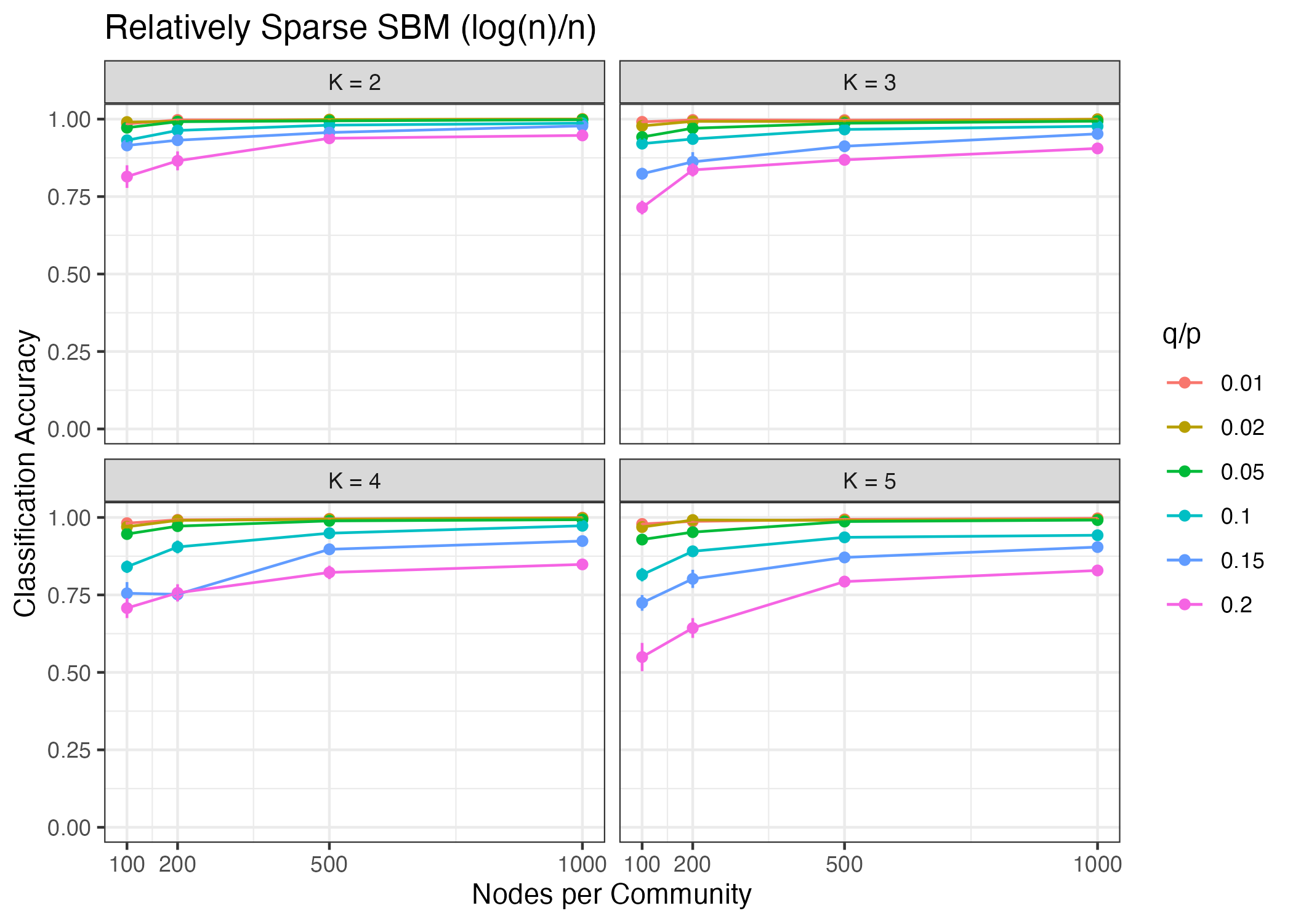
Figure S1: Classification accuracy using 10% of the node embeddings to learn a multinomial logistic regression classifier. Mean and one standard error shown.

Additional Results, Community Detection

Here we include additional simulation results which were omitted from the main text. In particular, for the simulations considered in the main manuscript we now examine the community recovery performance in terms of the adjusted rand index (ARI) [17]. We show the average ARI score across these simulations, along with error bars corresponding to one standard error. In each case, the ARI metric is similar to the proportion of nodes correctly recovered. As we increase the number of nodes this performance improves.

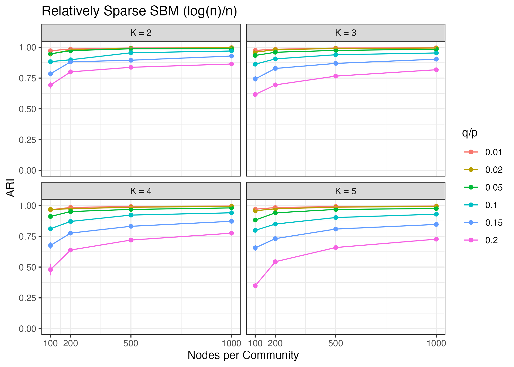
Figure S2: ARI for relatively sparse SBM. Mean and one standard error shown.

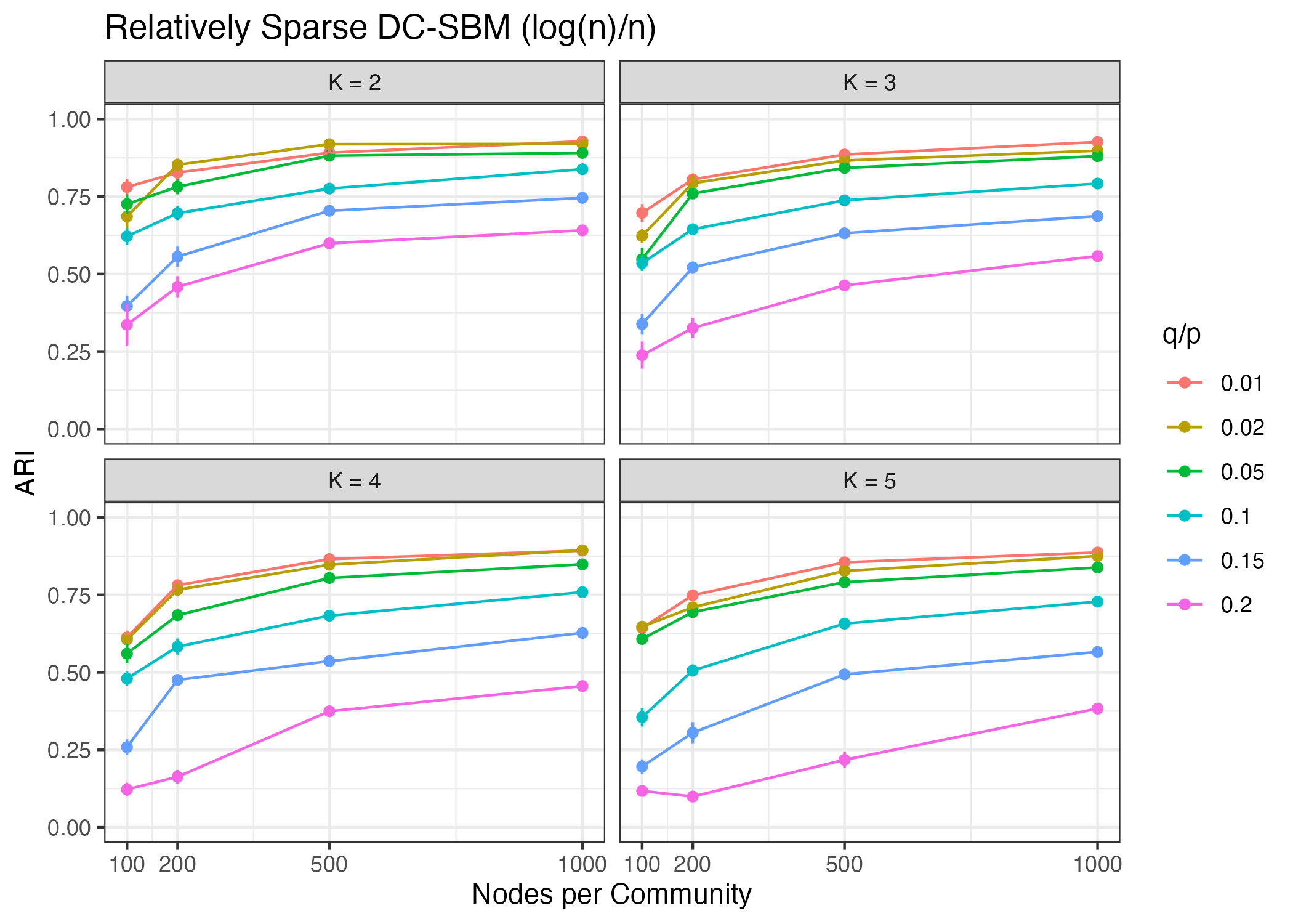
Figure S3: ARI for relatively sparse DC-SBM. Mean and one standard error shown.

Figure S4: ARI varying $\alpha$ for relatively sparse DC-SBM. Mean and one standard error shown.

Supplement References

References

• [1] Emmanuel Abbe β€œCommunity detection and stochastic block models: recent developments” In The Journal of Machine Learning Research 18.1 JMLR. org, 2017, pp. 6446–6531
• [2] Edoardo M Airoldi, David M. Blei, Stephen E. Fienberg and Eric P. Xing β€œMixed membership stochastic blockmodels” In Advances in neural information processing systems 21, 2008
• [3] Edoardo M Airoldi et al. β€œMixed membership stochastic block models for relational data with application to protein-protein interactions” In Proceedings of the international biometrics society annual meeting 15, 2006, pp. 1
• [4] Daniel Aloise, Amit Deshpande, Pierre Hansen and Preyas Popat β€œNP-hardness of Euclidean sum-of-squares clustering” In Machine Learning 75.2, 2009, pp. 245–248 DOI: 10.1007/s10994-009-5103-0
• [5] Peng Cui, Xiao Wang, Jian Pei and Wenwu Zhu β€œA survey on network embedding” In IEEE transactions on knowledge and data engineering 31.5 IEEE, 2018, pp. 833–852
• [6] Andrew Davison β€œAsymptotics of $\ell\_2$ Regularized Network Embeddings” In Advances in Neural Information Processing Systems 35, 2022, pp. 24960–24974
• [7] Andrew Davison and Morgane Austern β€œAsymptotics of Network Embeddings Learned via Subsampling” In Journal of Machine Learning Research 24.138, 2023, pp. 1–120
• [8] Shaofeng Deng, Shuyang Ling and Thomas Strohmer β€œStrong consistency, graph laplacians, and the stochastic block model” In The Journal of Machine Learning Research 22.1 JMLRORG, 2021, pp. 5210–5253
• [9] Linton Freeman β€œThe development of social network analysis” In A Study in the Sociology of Science 1.687, 2004, pp. 159–167
• [10] Chao Gao, Zongming Ma, Anderson Y. Zhang and Harrison H. Zhou β€œCommunity detection in degree-corrected block models” In The Annals of Statistics 46.5 Institute of Mathematical Statistics, 2018, pp. 2153–2185 DOI: 10.1214/17-AOS1615
• [11] Aditya Grover and Jure Leskovec β€œnode2vec: Scalable feature learning for networks” In Proceedings of the 22nd ACM SIGKDD international conference on Knowledge discovery and data mining, 2016, pp. 855–864
• [12] Will Hamilton, Zhitao Ying and Jure Leskovec β€œInductive representation learning on large graphs” In Advances in neural information processing systems 30, 2017
• [13] John A Hartigan and Manchek A Wong β€œAlgorithm AS 136: A k-means clustering algorithm” In Journal of the royal statistical society. series c (applied statistics) 28.1 JSTOR, 1979, pp. 100–108
• [14] Peter D Hoff, Adrian E Raftery and Mark S Handcock β€œLatent space approaches to social network analysis” In Journal of the american Statistical association 97.460 Taylor & Francis, 2002, pp. 1090–1098
• [15] Paul W Holland, Kathryn Blackmond Laskey and Samuel Leinhardt β€œStochastic blockmodels: First steps” In Social networks 5.2 Elsevier, 1983, pp. 109–137
• [16] Roger A. Horn and Charles R. Johnson β€œMatrix Analysis” New York, NY, USA: Cambridge University Press, 2012
• [17] Lawrence Hubert and Phipps Arabie β€œComparing partitions” In Journal of classification 2 Springer, 1985, pp. 193–218
• [18] Jiashun Jin, Zheng Tracy Ke, Shengming Luo and Minzhe Wang β€œOptimal estimation of the number of network communities” In Journal of the American Statistical Association Taylor & Francis, 2022, pp. 1–16
• [19] Brian Karrer and Mark EJ Newman β€œStochastic blockmodels and community structure in networks” In Physical review E 83.1 APS, 2011, pp. 016107
• [20] Vladimir Koltchinskii and Evarist GinΓ© β€œRandom Matrix Approximation of Spectra of Integral Operators” Number: 1 Publisher: International Statistical Institute (ISI) and Bernoulli Society for Mathematical Statistics and Probability In Bernoulli 6.1, 2000, pp. 113–167 DOI: 10.2307/3318636
• [21] Amit Kumar, Yogish Sabharwal and Sandeep Sen β€œLinear Time Algorithms for Clustering Problems in Any Dimensions” In Automata, Languages and Programming, Lecture Notes in Computer Science Berlin, Heidelberg: Springer, 2005, pp. 1374–1385 DOI: 10.1007/11523468_111
• [22] Pierre Latouche, Etienne BirmelΓ© and Christophe Ambroise β€œOverlapping stochastic block models with application to the French political blogosphere” In The Annals of Applied Statistics 5.1 Institute of Mathematical Statistics, 2011, pp. 309–336 DOI: 10.1214/10-AOAS382
• [23] Can M Le and Elizaveta Levina β€œEstimating the number of communities by spectral methods” In Electronic Journal of Statistics 16.1 The Institute of Mathematical Statisticsthe Bernoulli Society, 2022, pp. 3315–3342
• [24] Can M Le, Elizaveta Levina and Roman Vershynin β€œConcentration of random graphs and application to community detection” In Proceedings of the International Congress of Mathematicians: Rio de Janeiro 2018, 2018, pp. 2925–2943 World Scientific
• [25] Sirio Legramanti, Tommaso Rigon, Daniele Durante and David B Dunson β€œExtended stochastic block models with application to criminal networks” In The Annals of Applied Statistics 16.4, 2022, pp. 2369
• [26] Jing Lei β€œNetwork representation using graph root distributions” In The Annals of Statistics 49.2, 2021, pp. 745–768
• [27] Jing Lei and Alessandro Rinaldo β€œConsistency of spectral clustering in stochastic block models” In The Annals of Statistics 43.1 Institute of Mathematical Statistics, 2015, pp. 215–237 DOI: 10.1214/14-AOS1274
• [28] Keith D Levin et al. β€œLimit theorems for out-of-sample extensions of the adjacency and Laplacian spectral embeddings” In The Journal of Machine Learning Research 22.1 JMLRORG, 2021, pp. 8707–8765
• [29] Feng Luo et al. β€œModular organization of protein interaction networks” In Bioinformatics 23.2 Oxford University Press, 2007, pp. 207–214
• [30] Cong Ma, Yuanxin Li and Yuejie Chi β€œBeyond Procrustes: Balancing-free gradient descent for asymmetric low-rank matrix sensing” In IEEE Transactions on Signal Processing 69 IEEE, 2021, pp. 867–877
• [31] Shujie Ma, Liangjun Su and Yichong Zhang β€œDetermining the number of communities in degree-corrected stochastic block models” In The Journal of Machine Learning Research 22.1 JMLRORG, 2021, pp. 3217–3279
• [32] Tomas Mikolov et al. β€œDistributed representations of words and phrases and their compositionality” In Advances in neural information processing systems 26, 2013
• [33] Andrew Ng, Michael Jordan and Yair Weiss β€œOn spectral clustering: Analysis and an algorithm” In Advances in neural information processing systems 14, 2001
• [34] Bryan Perozzi, Rami Al-Rfou and Steven Skiena β€œDeepwalk: Online learning of social representations” In Proceedings of the 20th ACM SIGKDD international conference on Knowledge discovery and data mining, 2014, pp. 701–710
• [35] Jiezhong Qiu et al. β€œNetwork embedding as matrix factorization: Unifying deepwalk, line, pte, and node2vec” In Proceedings of the eleventh ACM international conference on web search and data mining, 2018, pp. 459–467
• [36] Herbert Robbins and Sutton Monro β€œA Stochastic Approximation Method” Number: 3 Publisher: Institute of Mathematical Statistics In The Annals of Mathematical Statistics 22.3, 1951, pp. 400–407 DOI: 10.1214/aoms/1177729586
• [37] P Rubin-Delanchy, CE Priebe, M Tang and J Cape β€œA statistical interpretation of spectral embedding: the generalised random dot product graph. arXiv e-prints” In arXiv preprint arXiv:1709.05506, 2017
• [38] Liangjun Su, Wuyi Wang and Yichong Zhang β€œStrong consistency of spectral clustering for stochastic block models” In IEEE Transactions on Information Theory 66.1 IEEE, 2019, pp. 324–338
• [39] Michel Talagrand β€œUpper and Lower Bounds for Stochastic Processes: Modern Methods and Classical Problems”, Ergebnisse der Mathematik und ihrer Grenzgebiete. 3. Folge / A Series of Modern Surveys in Mathematics Berlin Heidelberg: Springer-Verlag, 2014 DOI: 10.1007/978-3-642-54075-2
• [40] Stephen Tu et al. β€œLow-rank Solutions of Linear Matrix Equations via Procrustes Flow” ISSN: 1938-7228 In Proceedings of The 33rd International Conference on Machine Learning PMLR, 2016, pp. 964–973 URL: https://proceedings.mlr.press/v48/tu16.html
• [41] Victor Veitch et al. β€œEmpirical risk minimization and stochastic gradient descent for relational data” In The 22nd International Conference on Artificial Intelligence and Statistics, 2019, pp. 1733–1742 PMLR
• [42] Petar VeličkoviΔ‡ et al. β€œGraph attention networks” In arXiv preprint arXiv:1710.10903, 2017
• [43] Petar VeličkoviΔ‡ et al. β€œDeep Graph Infomax” arXiv: 1809.10341 In arXiv:1809.10341 [cs, math, stat], 2018 URL: http://arxiv.org/abs/1809.10341
• [44] Owen G Ward, Zhen Huang, Andrew Davison and Tian Zheng β€œNext waves in veridical network embedding” In Statistical Analysis and Data Mining: The ASA Data Science Journal 14.1 Wiley Online Library, 2021, pp. 5–17
• [45] Yi Yu, Tengyao Wang and Richard J Samworth β€œA useful variant of the Davis–Kahan theorem for statisticians” In Biometrika 102.2 Oxford University Press, 2015, pp. 315–323
• [46] Si Zhang, Hanghang Tong, Jiejun Xu and Ross Maciejewski β€œGraph convolutional networks: a comprehensive review” In Computational Social Networks 6.1 SpringerOpen, 2019, pp. 1–23
• [47] Yichi Zhang and Minh Tang β€œConsistency of random-walk based network embedding algorithms” In arXiv preprint arXiv:2101.07354, 2021
• [48] Zhihui Zhu, Qiuwei Li, Gongguo Tang and Michael B Wakin β€œThe global optimization geometry of low-rank matrix optimization” In IEEE Transactions on Information Theory 67.2 IEEE, 2021, pp. 1308–1331