Peccei-Quinn Inflation at the Pole
and Axion Kinetic Misalignment

Hyun Min Lee^1,†, Adriana G. Menkara^1,2,♯,
Myeong-Jung Seong^1,‡, and Jun-Ho Song^1,⋆

¹Department of Physics, Chung-Ang University, Seoul 06974, Korea.
²CERN, Theory department, 1211 Geneva 23, Switzerland.

We propose a minimal extension of the Standard Model with the Peccei-Quinn (PQ) scalar field and explain the relic density of the QCD axion through the kinetic misalignment with a relatively small axion decay constant. To this purpose, we consider a slow-roll inflation from the radial component of the PQ field with the PQ conserving potential near the pole of its kinetic term and investigate the post-inflationary dynamics of the PQ field for reheating. The angular mode of the PQ field, identified with the QCD axion, receives a nonzero velocity during inflation due to the PQ violating potential, evolving with an approximately conserved Noether PQ charge. We determine the reheating temperature from the perturbative decays and scattering processes of the inflaton and obtain dark radiation from the axions produced from the inflaton scattering at a testable level in the future Cosmic Microwave Background experiments. We show the correlation between the reheating temperature, the initial velocity of the axion and the axion decay constant, realizing the axion kinetic misalignment for the correct relic density.

^†Email: hminlee@cau.ac.kr

^♯Email: amenkara@cau.ac.kr

^‡Email: tjdaudwnd@gmail.com

^⋆Email: thdwnsgh1003@naver.com

1 Introduction

The QCD axion has been proposed to solve the strong CP problem as a pseudo-Goldstone boson appearing after an anomalous U(1) Peccei-Quinn (PQ) symmetry is broken spontaneously [1, 2, 3]. The QCD axion is also a good candidate for cold dark matter whose abundance is generated by the misalignment mechanism [4]. If the axion was once in thermal equilibrium due to a relatively high temperature of the universe, it could not be a dominant component for dark matter, but instead it provides a component for dark radiation [5, 6, 7], which is testable in the future experiments for Cosmic Microwave Background (CMB) anisotropies.

Recently, the general initial conditions with a nonzero velocity for the QCD axion or axion-like particles have been considered, under the name of the axion kinetic misalignment mechanism [8]. At the onset of the axion oscillation, the kinetic energy for the axion is comparable to the potential energy for the axion, so the axion abundance depends on the axion velocity initially set by the Noether PQ charge in the early universe. The PQ symmetry is broken explicitly by quantum gravity effects, so it naturally induces a nonzero velocity for the axion. However, since the overall magnitude of the PQ violating potential is set by the modulus of the PQ field, we need to take into account the dynamics of the PQ field in the early universe and make sure that the consistent picture with the axion kinetic misalignment at a later stage emerges.

In this article, we consider the extension of the SM with a PQ complex scalar field in the presence of the U(1) PQ symmetry. The angular component of the PQ field is identified as the QCD axion and the radial component of the PQ field is regarded as the saxion. The QCD anomalies are generated due to an extra vector-like quark as in the KSVZ axion model [2], providing the axion-gluon coupling necessary for the dynamical solution to the strong CP problem. In this model, we pursue the origin of the initial condition for the axion misalignment in the context of the PQ inflation at the pole [9, 10]. The saxion couples conformally to gravity, playing a role of the inflaton near the pole of the kinetic term in the Einstein frame. The dynamics of the saxion is dominated by the PQ conserving potential. On the other hand, we show that the PQ violating potential sets the initial velocity for the axion during inflation, and an approximately conserved Noether PQ charge is achievable at the end of reheating.

We compute a sufficiently large reheating temperature of the universe from the decays and scattering processes of the saxion and identify the dark radiation component from the axions produced by the saxion scattering. We show the condition for the successful axion kinetic misalignment in the parameter space for the reheating temperature, the initial velocity of the axion and the axion decay constant (or the axion mass).

The paper is organized as follows. We first present the model setup for the PQ inflation and the interactions of the PQ field to the extra vector-like quark, the SM Higgs, and possibly to the right-handed neutrinos. In this model, we discuss the Einstein-frame potential, the bounds on the PQ violating potential from the axion quality and the axion-photon coupling. Next we discuss the inflationary dynamics depending on whether inflation is driven by the PQ conserving or violating potentials, and describe the post-inflationary dynamics of the inflaton and the axion from the classical equations of motion. We continue to consider the reheating period in the presence of the decays and scattering processes of the inflaton and determine the reheating temperature as well as the dark radiation from the axions accordingly. From the initial axion velocity given at the end of inflation, we show the evolution of the axion velocity to the present and find the parameter space where the axion kinetic alignment is a dominant production mechanism for axion dark matter. Finally, conclusions are drawn.

2 The setup

We introduce a complex scalar field $\Phi$, which is charged under the U(1) PQ symmetry. We assume that the PQ field is conformally coupled to gravity [10], but the conformal symmetry is broken by the mass term for the PQ field and the higher order interactions in the PQ potential. Then, we consider the Jordan-frame Lagrangian for the PQ inflation as

$$\frac{{\cal L}_{J}}{\sqrt{-g_{J}}}=-\frac{1}{2}M^{2}_{P}\,\Omega(\Phi)R(g_{J})+|\partial_{\mu}\Phi|^{2}-\Omega^{2}(\Phi)V_{E}(\Phi)$$ (1)

where the non-minimal coupling function and the PQ potential are taken to

$$\Omega(\Phi) = 1-\frac{1}{3M^{2}_{P}}|\Phi|^{2},$$ (2)

$$V_{E}(\Phi) = V^{\prime}_{0}+\frac{\beta_{m}}{M^{2m-4}_{P}}|\Phi|^{2m}-m^{2}_{\Phi}|\Phi|^{2}+\bigg{(}\sum_{k=0}^{[n/2]}\frac{c_{k}}{2M^{n-4}_{P}}\,|\Phi|^{2k}\Phi^{n-2k}+{\rm h.c.}\bigg{)}.$$ (3)

Here, $V_{0}$ is the cosmological constant, $\beta_{m}$ is a PQ conserving dimensionless parameter, $c_{k}$ are dimensionless parameters, parametrizing the explicit breaking of the PQ symmetry at the Planck scale [11] in the general form of order $n>4$, and $[n/2]$ is the largest integer smaller than $n/2$. The PQ violating terms of order higher than $n$ can be added, but we assume that they are suppressed for the inflaton or axion potentials.

For $m=2$, we can recast the PQ conserving part of the potential in eq. (3) into

$$V_{\rm PQ}=V_{0}+\lambda_{\Phi}\bigg{(}|\Phi|^{2}-\frac{f^{2}_{a}}{2}\bigg{)}^{2}$$ (4)

where the parameters are redefined as $\beta_{m}=\lambda_{\Phi}$, $m^{2}_{\phi}=\lambda_{\Phi}f^{2}_{a}$ and $V^{\prime}_{0}=V_{0}+\frac{1}{4}\lambda_{\Phi}f^{4}_{a}$.

In the KSVZ models [2], it is necessary to introduce the Yukawa coupling of the PQ field to a vector-like extra quark $Q$ for the QCD anomalies, as follows,

$${\cal L}_{Q,{\rm int}}=-y_{Q}\Phi{\bar{Q}}_{R}Q_{L}+{\rm h.c.}$$ (5)

where $Q_{L},Q_{R}$ carries $+1$ and $-1$ and $\Phi$ carries $-2$ under the $U(1)_{\rm PQ}$ symmetry. We can also introduce a Higgs-portal quartic coupling between the SM Higgs and the PQ field, as follows,

$$\Delta V_{E}=\lambda_{H\Phi}|\Phi|^{2}|H|^{2}.$$ (6)

As a consequence, the Higgs-portal quartic coupling and the Yukawa couplings for the PQ field are crucial for the decays or scattering of the saxion inflaton after inflation and determining the reheating temperature, as will be discussed in the later section.

We also comment on the possibility that right-handed neutrinos, $N_{i}(i=1,2,3)$, carry PQ charge $+1$, and they receive masses after the PQ symmetry is broken. In this case, we can also introduce extra Yukawa couplings of the PQ field for the Majorana masses of the right-handed neutrinos as

$${\cal L}_{N,{\rm int}}=-\frac{1}{2}\lambda_{N}\Phi\overline{N^{c}_{L}}N_{R}+{\rm h.c.}.$$ (7)

Then, in order to generate neutrino masses by seesaw mechanism, we need to include the Yukawa couplings between the right-handed neutrinos and the SM lepton doublets by ${\cal L}_{\rm seesaw}=-y_{N}{\tilde{H}}{\bar{l}}_{L}N_{R}+{\rm h.c.}$, so we need to assign a PQ charge $+1$ to the lepton doublets. But, we can assign the vector-like PQ charges for the SM charged leptons, so they do not contribute to the electromagnetic anomalies for the PQ symmetry. If the right-handed neutrinos are neutral under the PQ symmetry, the right-handed neutrinos couple to the PQ field by non-renormalizable interactions or through the graviton exchanges.

2.1 Einstein frame Lagrangian

After making a Weyl transformation of the metric by $g_{J,\mu\nu}=g_{E,\mu\nu}/\Omega$ with $\Omega=1-\frac{1}{3M^{2}_{P}}|\Phi|^{2}$, we obtain the Einstein-frame Lagrangian as follows,

$$\frac{{\cal L}_{E}}{\sqrt{-g_{E}}} = -\frac{1}{2}M^{2}_{P}R(g_{E})+\frac{|\partial_{\mu}\Phi|^{2}}{\big{(}1-\frac{1}{3M^{2}_{P}}|\Phi|^{2}\big{)}^{2}}$$ (8)

$$-\frac{1}{3M^{2}_{P}\big{(}1-\frac{1}{3M^{2}_{P}}|\Phi|^{2}\big{)}^{2}}\bigg{(}|\Phi|^{2}|\partial_{\mu}\Phi|^{2}-\frac{1}{4}\partial_{\mu}|\Phi|^{2}\partial^{\mu}|\Phi|^{2}\bigg{)}-V_{E}(\Phi).$$

We take the PQ field in the polar coordinate representation,

$$\Phi=\frac{1}{\sqrt{2}}\,\rho\,e^{i\theta}$$ (9)

where $\rho,\theta$ are radial and angular modes of the PQ field, respectively. Then, choosing $m=2$ for the PQ conserving potential in eq. (3), we get the Einstein-frame Lagrangian for the radial mode $\rho$ and the angular mode $\theta$ as

$$\frac{{\cal L}_{E}}{\sqrt{-g_{E}}}=-\frac{1}{2}M^{2}_{P}R+\frac{1}{2}\,\frac{(\partial_{\mu}\rho)^{2}}{\big{(}1-\frac{1}{6M^{2}_{P}}\rho^{2}\big{)}^{2}}+\frac{1}{2}\frac{\rho^{2}(\partial_{\mu}\theta)^{2}}{\big{(}1-\frac{1}{6M^{2}_{P}}\rho^{2}\big{)}}-V_{E}(\rho,\theta)$$ (10)

where

$$V_{E}(\rho,\theta)=V_{0}+\frac{1}{4}\lambda_{\Phi}(\rho^{2}-f^{2}_{a})^{2}+\frac{\rho^{n}}{2^{n/2}M^{n-4}_{P}}\sum_{k=0}^{[n/2]}|c_{k}|\,\cos\Big{(}(n-2k)\theta+A_{k}\Big{)},$$ (11)

with $c_{k}=|c_{k}|e^{iA_{k}}$. Making the kinetic term for the radial mode canonically normalized by

$$\rho=\sqrt{6}M_{P}\tanh\Big{(}\frac{\phi}{\sqrt{6}M_{P}}\Big{)},$$ (12)

we rewrite the Einstein-frame Lagrangian in eq. (10) as

$$\frac{{\cal L}_{E}}{\sqrt{-g_{E}}}=-\frac{1}{2}M^{2}_{P}R+\frac{1}{2}(\partial_{\mu}\phi)^{2}+3M^{2}_{P}\sinh^{2}\Big{(}\frac{\phi}{\sqrt{6}M_{P}}\Big{)}\,(\partial_{\mu}\theta)^{2}-V_{E}(\phi,\theta),$$ (13)

where

$$V_{E}(\phi,\theta) = V_{\rm PQ}(\phi)+V_{\rm PQV}(\rho,\theta),$$ (14)

with

$$V_{\rm PQ}(\phi) = V_{0}+\frac{1}{4}\lambda_{\Phi}\Big{(}6M^{2}_{P}\tanh^{2}\Big{(}\frac{\phi}{\sqrt{6}M_{P}}\Big{)}-f^{2}_{a}\Big{)}^{2},$$ (15)

$$V_{\rm PQV}(\rho,\theta) = 3^{n/2}M^{4}_{P}\tanh^{n}\Big{(}\frac{\phi}{\sqrt{6}M_{P}}\Big{)}\sum_{k=0}^{[n/2]}|c_{k}|\cos\Big{(}(n-2k)\theta+A_{k}\Big{)}.$$ (16)

We can also take the VEV of the PQ field in the true vacuum to satisfy $6M^{2}_{P}\tanh^{2}\big{(}\frac{\langle\phi\rangle}{\sqrt{6}M_{P}}\big{)}\simeq f^{2}_{a}$, so $\langle\rho\rangle\sim\langle\phi\rangle\sim f_{a}$ for $f_{a}\ll M_{P}$. After the angular mode gets a VEV $\langle\theta\rangle$, we can get an observed tiny cosmological constant by tuning the bare cosmological constant $V_{0}$ to cancel the vacuum energy coming from the PQ breaking terms, as follows,

$$V_{0}\simeq-M^{4}_{P}\bigg{(}\frac{f_{a}}{\sqrt{2}M_{P}}\bigg{)}^{n}\,\sum_{k=0}^{[n/2]}|c_{k}|\cos\Big{(}(n-2k)\langle\theta\rangle+A_{k}\Big{)}.$$ (17)

Moreover, the kinetic term for the axion in the true vacuum becomes $3M^{2}_{P}\sinh^{2}\big{(}\frac{\langle\phi\rangle}{\sqrt{6}M_{P}}\big{)}\,(\partial_{\mu}\theta)^{2}\simeq\frac{1}{2}f^{2}_{a}\,(\partial_{\mu}\theta)^{2}$, so we can take the canonical axial mode as $a=f_{a}\,\theta$, which is identified as the axion solving the strong CP problem.

For a general PQ conserving potential, we note that it takes the following form for the canonical radial mode in the Einstein frame,

$$V_{\rm PQ}(\phi)=V^{\prime}_{0}+3^{m}\beta_{m}M^{4}_{P}\bigg{[}\tanh\Big{(}\frac{\phi}{\sqrt{6}M_{P}}\Big{)}\bigg{]}^{2m}-3m^{2}_{\Phi}M^{2}_{P}\tanh^{2}\Big{(}\frac{\phi}{\sqrt{6}M_{P}}\Big{)}.$$ (18)

In this case, for $\phi\ll\sqrt{6}M_{P}$, we can obtain the VEV of the PQ field in the true vacuum from $2m\beta_{m}\phi^{2m-1}/(2^{m}M^{2m-4}_{P})=m^{2}_{\Phi}\phi$, that is, $\langle\rho\rangle\sim\langle\phi\rangle\sim f_{a}=(m^{2}_{\Phi}M^{2m-4}_{P})^{1/(2m-2)}$. For instance, for $m=3$, we get the VEV of the PQ field as $f_{a}=\sqrt{m_{\Phi}M_{P}}$.

2.2 Axion quality problem

In the presence of the PQ anomalies, we get the effective gluon couplings violating the strong CP, as follows,

$${\cal L}_{\rm gluons}=\frac{g^{2}_{s}}{32\pi^{2}}\Big{(}{\bar{\theta}}+\xi\frac{a}{f_{a}}\Big{)}G^{a}_{\mu\nu}{\tilde{G}}^{a\mu\nu}$$ (19)

where $\xi$ is the PQ anomaly coefficient, which is set to $\xi=1$ in KSVZ models. Then, after the QCD phase transition, there appears an extra contribution to the axion potential [11], in the following form,

$$\Delta V_{E}=-\Lambda^{4}_{\rm QCD}\cos\Big{(}{\bar{\theta}}+\xi\frac{a}{f_{a}}\Big{)}.$$ (20)

After the radial mode settles down to the minimum of the potential, i.e. $\langle\rho\rangle\simeq f_{a}$, from eqs. (14) and (20), the effective potential for the axion after the QCD phase transition is given by

$$V_{\rm eff}(a)=V_{0}-\Lambda^{4}_{\rm QCD}\cos\Big{(}{\bar{\theta}}+\xi\frac{a}{f_{a}}\Big{)}+M^{4}_{P}\bigg{(}\frac{f_{a}}{\sqrt{2}M_{P}}\bigg{)}^{n}\,\sum_{k=0}^{[n/2]}|c_{k}|\cos\Big{(}(n-2k)\frac{a}{f_{a}}+A_{k}\Big{)}.$$ (21)

In order to solve the strong CP problem by the axion, the axion potential needs to relax the effective $\theta$ term dynamically to satisfy the EDM bound,

$$|\theta_{\rm eff}|=\bigg{|}{\bar{\theta}}+\xi\frac{\langle a\rangle}{f_{a}}\bigg{|}<10^{-10}.$$ (22)

Then, from the minimization of the effective potential for the axion in eq. (21), namely, $\frac{dV_{\rm eff}}{da}=0$, we obtain

$$a_{\rm phys}\equiv a+\frac{f_{a}}{\xi}{\bar{\theta}}\simeq\frac{f^{n-1}_{a}}{2^{n/2}M^{n-4}_{P}m^{2}_{a}}\,\sum_{k=0}^{[n/2]}|c_{k}|(n-2k)\sin\Big{(}A_{k}-\frac{n-2k}{\xi}\,{\bar{\theta}}\Big{)}$$ (23)

where $m^{2}_{a}=\frac{\xi^{2}}{f^{2}_{a}}\,\Lambda^{4}_{\rm QCD}$ is the squared mass for the axion due to QCD only, and we assumed $(n-2k)\frac{a_{\rm phys}}{f_{a}}\ll 1$ and $(n-2k)^{2}|c_{k}|f^{n-2}_{a}/(2^{n/2}M^{n-4}_{P})\cos\big{(}A_{k}-\frac{n-2k}{\xi}\,{\bar{\theta}}\big{)}\lesssim m^{2}_{a}$ for all $k$.

As a result, from eq. (23) with eq. (22), we can solve the strong CP problem if

$$\frac{\xi f^{n-2}_{a}}{2^{n/2}M^{n-4}_{P}m^{2}_{a}}\,\sum_{k=0}^{[n/2]}|c_{k}|(n-2k)\sin\Big{(}A_{k}-\frac{n-2k}{\xi}\,{\bar{\theta}}\Big{)}<10^{-10}.$$ (24)

Unless there is a cancellation between various contributions at the same order, each term in the PQ violating potential is constrained by

$$\bigg{(}\frac{f_{a}}{M_{P}}\bigg{)}^{n}\lesssim\frac{2^{n/2}\xi}{(n-2k)|c_{k}|}\bigg{(}\frac{\Lambda_{\rm QCD}}{M_{P}}\bigg{)}^{4}.$$ (25)

Then, for a given axion decay constant $f_{a}$, we can bound the order of the PQ violating polynomial. For instance, for $f_{a}=10^{12}\,{\rm GeV}$, $\xi=1$ and $|c_{k}|={\cal O}(1)$, we need $n\gtrsim 12$ for the axion quality. In general, the lower bound on the order of the PQ violating polynomial scales by $n\propto 1/\ln(M_{P}/f_{a})$. So, for $f_{a}=10^{6}\,{\rm GeV}$, we need $n\gtrsim 6$.

However, considering the bound from the CMB normalization in our model, as will be seen in the later section, the coefficient of the PQ violating term is bounded by $3^{n/2}|c_{k}|\lesssim 10^{-10}$ for all $k$. Thus, it is sufficient to take $n\gtrsim 10(5)$ for $f_{a}=10^{12}(10^{6})\,{\rm GeV}$, $\xi=1$ and $|c_{k}|\lesssim 10^{-12}$.

2.3 Axion-photon coupling

In the presence of charged fermions with nonzero PQ charges, we also obtain the effective axion-photon coupling below the PQ symmetry breaking scale, as follows,

$${\cal L}_{\rm photon}=\frac{1}{4}g_{a\gamma\gamma}\,F_{\mu\nu}{\tilde{F}}^{\mu\nu}$$ (26)

with

$$g_{a\gamma\gamma}=\frac{\alpha}{2\pi f_{a}/\xi}\bigg{(}\frac{E}{N}-1.92\bigg{)}.$$ (27)

In the minimal scenario where the QCD anomalies for the PQ symmetry are originated from an extra heavy quark with zero electric charge, we get $\xi=1$ and $E/N=0$.

3 Inflationary dynamics

In this section, we discuss the inflationary predictions and bounds in the pole inflation for the PQ field. We divide our discussion into two cases, depending on whether the PQ violating terms are relevant for inflation or not: inflation with PQ conservation and inflation with PQ violation. We note that there were similar proposals for the inflation scenarios based on the PQ field, but with the non-minimal coupling taken to be different from the conformal coupling [12, 13, 14].

3.1 Inflaton equations

First, from eq. (13), we obtain the equation of motion for the radial mode in the following,

$${\ddot{\phi}}+3H{\dot{\phi}}-\sqrt{6}M_{P}\,\sinh\Big{(}\frac{\phi}{\sqrt{6}M_{P}}\Big{)}\cosh\Big{(}\frac{\phi}{\sqrt{6}M_{P}}\Big{)}\,{\dot{\theta}}^{2}=-\frac{\partial V_{E}}{\partial\phi}.$$ (28)

Thus, for a slow-roll inflation with ${\ddot{\phi}}\ll H{\dot{\phi}}$ and ${\dot{\theta}}\ll H$, we simply get

$${\dot{\phi}}\simeq-\frac{1}{3H}\frac{\partial V_{E}}{\partial\phi}=-\sqrt{2\epsilon_{\phi}}\,M_{P}H$$ (29)

where $\epsilon_{\phi}$ is the slow-roll parameter for the radial mode, given by $\epsilon_{\phi}=\frac{M^{2}_{P}}{2V^{2}_{E}}\big{(}\frac{\partial V_{E}}{\partial\phi}\big{)}^{2}$. Here, the Hubble parameter is determined by

$$H^{2}=\frac{1}{3M^{2}_{P}}\,\bigg{(}\frac{1}{2}(\partial_{\mu}\phi)^{2}+3M^{2}_{P}\sinh^{2}\Big{(}\frac{\phi}{\sqrt{6}M_{P}}\Big{)}\,(\partial_{\mu}\theta)^{2}+V_{E}\bigg{)}.$$ (30)

which is approximate to $H^{2}\simeq\frac{V_{E}}{3M^{2}_{P}}$ during inflation.

Moreover, from eq. (13), we also obtain the equation of motion for the axial mode during inflation as

$$6M^{2}_{P}\sinh^{2}\Big{(}\frac{\phi}{\sqrt{6}M_{P}}\Big{)}\bigg{[}{\ddot{\theta}}+3H{\dot{\theta}}+\frac{2}{\sqrt{6}M_{P}}\coth\Big{(}\frac{\phi}{\sqrt{6}M_{P}}\Big{)}\,{\dot{\phi}}\,{\dot{\theta}}\bigg{]}=-\frac{\partial V_{E}}{\partial\theta}.$$ (31)

Then, taking ${\ddot{\theta}}\ll H{\dot{\theta}}$ and ${\dot{\phi}}\ll H$ for a slow-roll inflation, we obtain the approximate equation for the axion kinetic misalignment by

$${\dot{\theta}}\simeq-\frac{1}{3H}\,\frac{\frac{\partial V_{E}}{\partial\theta}}{6M^{2}_{P}\sinh^{2}\big{(}\frac{\phi}{\sqrt{6}M_{P}}\big{)}}=-\frac{\sqrt{2\epsilon_{\theta}}\,H}{6\sinh^{2}\big{(}\frac{\phi}{\sqrt{6}M_{P}}\big{)}}$$ (32)

where $\epsilon_{\theta}$ is the slow-roll parameter for the angular mode in the second equality, namely, $\epsilon_{\theta}=\frac{1}{2V^{2}_{E}}\big{(}\frac{\partial V_{E}}{\partial\theta}\big{)}^{2}$. Therefore, as compared to the velocity of the radial mode in eq. (29), the velocity of the angular mode has an extra suppression factor due to the non-canonical kinetic term during inflation where $\phi\gg\sqrt{6}M_{P}$. We can set the initial kinetic misalignment of the axion by using eq. (32) at the end of inflation.

For a slow-roll inflation, we need to take $\rho\sim\sqrt{6}M_{P}\gg f_{a}$ and ignore the bare cosmological constant in eq. (14). Then, the potential for inflation is approximated to

$$V_{E}(\phi,\theta)\simeq 9\lambda_{\Phi}M^{4}_{P}\tanh^{4}\Big{(}\frac{\phi}{\sqrt{6}M_{P}}\Big{)}+V_{n}(\theta)\tanh^{n}\Big{(}\frac{\phi}{\sqrt{6}M_{P}}\Big{)},$$ (33)

with

$$V_{n}(\theta)\equiv 3^{n/2}M^{4}_{P}\sum_{k=0}^{[n/2]}|c_{k}|\cos\Big{(}(n-2k)\theta+A_{k}\Big{)}.$$ (34)

3.2 Inflation with PQ conservation

We take the inflaton potential in eq. (33) to be dominated by the PQ conserving term in the following,

$$V_{E}(\phi)\simeq V_{I}\bigg{[}\tanh\Big{(}\frac{\phi}{\sqrt{6}M_{P}}\Big{)}\bigg{]}^{2m},$$ (35)

with $V_{I}\equiv 3^{m}\beta_{m}M^{4}_{P}$. Then, we first obtain the slow-roll parameters [10],

$$\epsilon = \frac{M^{2}_{P}}{2}\bigg{(}\frac{1}{V_{E}}\frac{\partial V_{E}}{\partial\phi}\bigg{)}^{2}$$ (36)

$$= \frac{4}{3}m^{2}\bigg{[}\sinh\Big{(}\frac{2\phi}{\sqrt{6}M_{P}}\Big{)}\bigg{]}^{-2},$$

$$\eta = \frac{M^{2}_{P}}{V_{E}}\frac{\partial^{2}V_{E}}{\partial\phi^{2}}$$ (37)

$$= -\frac{4}{3}m\bigg{[}\cosh\Big{(}\frac{2\phi}{\sqrt{6}M_{P}}\Big{)}-4\bigg{]}\bigg{[}\sinh\Big{(}\frac{2\phi}{\sqrt{6}M_{P}}\Big{)}\bigg{]}^{-2}.$$

The number of efoldings is

$$N = \frac{1}{M_{P}}\int^{\phi_{*}}_{\phi_{e}}\frac{{\rm sgn}(V^{\prime}_{E})d\phi}{\sqrt{2\epsilon}}$$ (38)

$$= \frac{3}{4m}\,\bigg{[}\cosh\Big{(}\frac{2\phi_{*}}{\sqrt{6}M_{P}}\Big{)}-\cosh\Big{(}\frac{2\phi_{e}}{\sqrt{6}M_{P}}\Big{)}\bigg{]}$$

where $\phi_{*},\phi_{e}$ are the values of the Higgs boson at horizon exit and the end of inflation, respectively. Here, we note that $\epsilon=1$ determines $\phi_{e}$. As a result, using eqs. (36), (37) and (38) and $N\simeq\frac{3}{8}\,\cosh\Big{(}\frac{2\phi_{*}}{\sqrt{6}M_{P}}\Big{)}$ for $\phi_{*}\gg\sqrt{6}M_{P}$ during inflation, we obtain the slow-roll parameters at horizon exit in terms of the number of efoldings as

$$\epsilon_{*} \simeq \frac{3}{4\big{(}N^{2}-\frac{9}{16m^{2}}\big{)}},$$ (39)

$$\eta_{*} \simeq \frac{3-2N}{2\big{(}N^{2}-\frac{9}{16m^{2}}\big{)}}.$$ (40)

Thus, we get the spectral index in terms of the number of efoldings, as follows,

$$n_{s} = 1-6\epsilon_{*}+2\eta_{*}$$ (41)

$$= 1-\frac{4N+3}{2\big{(}N^{2}-\frac{9}{16m^{2}}\big{)}}.$$

Moreover, the tensor-to-scalar ratio at horizon exit is

$$r=16\epsilon_{*}=\frac{12}{N^{2}-\frac{9}{16m^{2}}}.$$ (42)

As a result, from eq. (41), we obtain the spectral index as $n_{s}=0.966$ for $N=60$ being insensitive to $m$, which agrees with the observed spectral index from Planck, $n_{s}=0.967\pm 0.0037$ [15]. Moreover, we also predict the tensor-to-scalar ratio as $r=0.0033$ for $N=60$, which is again compatible with the bound from the combined Planck and Keck data [16], $r<0.036$.

The CMB normalization, $A_{s}=\frac{1}{24\pi^{2}}\frac{V_{I}}{\epsilon_{*}M^{4}_{P}}=2.1\times 10^{-9}$, bounds the quartic coupling for the PQ field by

$$3^{m}\beta_{m}=(3.1\times 10^{-8})\,r=1.0\times 10^{-10}$$ (43)

where we took $r=0.0033$, in the second equality. For instance, for $m=2$, we have $\beta_{m}=\lambda_{\Phi}$, so we need to impose $\lambda_{\Phi}=1.1\times 10^{-11}$ during inflation. Moreover, the inflation with PQ conservation sets the bound on the PQ violating terms, as follows,

$$V_{n}(\theta_{i})/M^{4}_{P}=3^{n/2}\sum_{k=0}^{[n/2]}|c_{k}|\cos\Big{(}(n-2k)\theta_{i}+A_{k}\Big{)}<1.0\times 10^{-10}.$$ (44)

3.3 Inflation with PQ violation

We take the case where the inflaton potential is dominated by the PQ violating terms in the following,

$$V_{E}(\phi,\theta)\simeq V_{n}(\theta)\cdot W_{n}(\phi).$$ (45)

with

$$W_{n}(\phi)\equiv\bigg{[}\tanh\Big{(}\frac{\phi}{\sqrt{6}M_{P}}\Big{)}\bigg{]}^{n}.$$ (46)

In this case, as far as the inflaton potential is positive definite during inflation, both the radial and angular modes of the PQ field could serve as the inflaton, corresponding to a multi-field inflation scenario [20]. Generically, the angular mode should not be located at the minimum of the potential during inflation. The reason is the following. For instance, taking $A_{k}$ in eq. (33) to be the same for all $k$, $V_{n}(\theta)$ becomes always negative at the minimum of the potential, so it would be not appropriate for inflation with PQ violation.

Even if the PQ violating terms can be dominant during inflation, they become sub-dominant as the PQ field evolves after inflation, such that the PQ conserving term takes over in determining the dynamics of the radial mode of the PQ field. Then, from the initial condition that the axial mode is deviated from the minimum during inflation, the axion can settle down safely toward the minimum of the potential after inflation.

For inflation with PQ violation, the slow-roll parameters are determined from the derivatives of the PQ violating terms in the potential, so $\epsilon_{\phi}\simeq\frac{M^{2}_{P}}{2W^{2}_{n}}\big{(}\frac{\partial W_{n}}{\partial\phi}\big{)}^{2}$ and $\epsilon_{\theta}\simeq\frac{1}{2V^{2}_{n}}\big{(}\frac{\partial V_{n}}{\partial\theta}\big{)}^{2}$. In this case, the slow-roll parameter for the radial mode is still small for $\phi\gg\sqrt{6}M_{P}$, but the slow-roll parameter for the angular mode is of order one. Nonetheless, the velocity of the angular mode is sufficiently small for $\phi\gg\sqrt{6}M_{P}$ due to its non-canonical kinetic term as can be seen in eq. (32). For generality, we can introduce the effective slow-roll parameter by taking into account the non-canonical kinetic term [20], as follows,

$$\epsilon=g^{\phi\phi}\epsilon_{\phi}+g^{\theta\theta}\epsilon_{\theta}$$ (47)

with $g^{\phi\phi}=1$ and $g^{\theta\theta}=1/\big{[}6M^{2}_{P}\sinh^{2}\big{(}\frac{\phi}{\sqrt{6}M_{P}}\big{)}\big{]}$.

When the inflation energy from the PQ violating terms is set for the axion field value set to $\theta=\theta_{i}$ during inflation, we obtain the constraint from the CMB normalization as

$$V_{n}(\theta_{i})=3^{n/2}\sum_{k=0}^{[n/2]}|c_{k}|\cos\Big{(}(n-2k)\theta_{i}+A_{k}\Big{)}=(3.1\times 10^{-8})\,r$$ (48)

where $r=16\epsilon_{*}$ with $\epsilon_{*}$ being evaluated from eq. (47) at the horizon exit.

3.4 Post-inflationary evolution of the fields

After inflation, the radial mode takes a sub-Planckian field value with $\phi\ll\sqrt{6}M_{P}$ so we can approximate the equations of motion in eqs. (28) and (31), as follows,

$${\ddot{\phi}}+3H{\dot{\phi}}-\phi\,{\dot{\theta}}^{2} \simeq -\frac{\partial V_{E}}{\partial\phi},$$ (49)

$$\phi^{2}({\ddot{\theta}}+3H{\dot{\theta}})+2\phi{\dot{\phi}}\,{\dot{\theta}} \simeq -\frac{\partial V_{E}}{\partial\theta}$$ (50)

where the Einstein-frame potential in eq. (14) becomes

$$V_{E}\simeq V_{0}+\frac{1}{4}\lambda_{\Phi}(\phi^{2}-f^{2}_{a})^{2}+\frac{1}{2^{n/2}}\bigg{(}\frac{\phi}{M_{P}}\bigg{)}^{n}M^{4}_{P}\sum_{k=0}^{[n/2]}|c_{k}|\cos\Big{(}(n-2k)\theta+A_{k}\Big{)}.$$ (51)

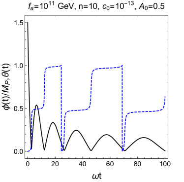
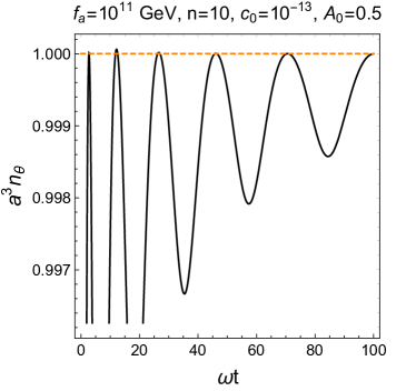
Figure 1: (Left) Post-inflationary evolution of the PQ inflaton and the angular mode as a function of $\omega t$ in black solid and blue dashed lines, respectively, with $\omega$ being the oscillation frequency of the inflaton condensate. (Right) Post-inflationary evolution of the total PQ Noether charge, $n_{\theta}=\phi^{2}{\dot{\theta}}$, as a function of $\omega t$. We considered the quartic term for the PQ-invariant potential and took $f_{a}=10^{11}\,{\rm GeV}$ and the parameters in the PQ violating potential to $n=10$, $c_{0}=10^{-13}$, $A_{0}=0.5$, and $c_{k}=0$ for $k\neq 0$.

We consider the case where the PQ conserving term is dominant for inflation. Then, as the amplitude of the radial mode decreases until reaching the VEV, the PQ violating terms become less important. When the PQ violating terms are sufficiently small during the evolution of the fields, we have the Noether charge for the PQ symmetry [8] approximately conserved after inflation. Namely, for $n_{\theta}=\phi^{2}{\dot{\theta}}$, we get $\frac{d}{dt}(a^{3}n_{\theta})=0$ from eq. (50). Thus, we can approximate the equation of motion for the radial mode in eq. (49) for $f_{a}\lesssim\phi\ll M_{P}$ as

$${\ddot{\phi}}+3H{\dot{\phi}}\simeq\frac{C^{2}}{a^{6}\phi^{3}}-\lambda_{\Phi}\phi^{3}$$ (52)

where $C=a_{e}^{3}\phi^{2}_{e}{\dot{\theta}}_{e}$ is the integration of constant given at the end of inflation. Therefore, the centrifugal force term due to the angular motion decreases rapidly as the universe is expanding, so the radial mode undergoes a coherent motion around the vacuum dominantly by the quartic term during reheating.

In Fig. 1, considering the PQ invariant quartic potential, we depict the time evolution of the PQ inflaton and the angular mode on left and the total PQ Noether charge on right as a function of $\omega t$. We took $f_{a}=10^{11}\,{\rm GeV}$, and the parameters in the PQ violating potential to $n=10$, $c_{0}=10^{-13}$, $A_{0}=0.5$, and $c_{k}=0$ for $k\neq 0$. We show that the PQ inflaton undergoes a damped oscillation dominated by the PQ invariant potential from the left figure, and the total PQ Noether charge oscillates but it approaches to the constant value, which is set by the initial condition during inflation.

We also remark on the case where PQ violating terms are dominant for inflation. In this case, the PQ violating terms are still important in the post-inflationary dynamics, so the Noether current for the PQ symmetry evolves nontrivially during reheating, so we need to solve two coupled equations of motion in eqs. (49) and (50), with $V_{E}\simeq V_{n}(\theta)\cdot W_{n}(\phi)$, for the post-inflationary evolution of the PQ field.

4 Reheating

We consider the inflaton condensate and the general equation of state during reheating. Then, we first discuss the perturbative reheating from the decay or scattering of the PQ inflaton into the extra fermions and the Higgs and determine the minimal reheating temperature.

4.1 Inflaton condensate

Suppose that the reheating dynamics is dominated by the radial mode of the PQ field. Then, for $|\Phi|\ll\sqrt{3}M_{P}$, we can approximate the kinetic term for the radial mode of the PQ field in Einstein frame in a canonical form, that is, $\phi\simeq\rho$, so the Einstein-frame potential for the pole inflation in eqs. (35) takes

$$V_{E}(\phi)\simeq\alpha_{m}\phi^{2m},$$ (53)

with $\alpha_{m}=\beta_{m}M^{4-2m}_{P}/2^{m}$. For $m=2$, we get $\beta_{m}=\lambda_{\Phi}$. Thus, as the inflaton potential becomes anharmonic for $m>1$ during reheating, we get a general equation of state during reheating. After the period of exponential expansion, the inflaton $\phi$ begins to oscillate about the minimum of the potential. For the inflaton potential given in eq. (35), the inflation field value at the end of inflation is determined by $\ddot{a}=0$ [10] to be

$$\phi_{\rm end} \simeq\sqrt{\frac{3}{8}}M_{P}\ln\left[\frac{1}{2}+\frac{2m}{3}\left(2m+\sqrt{4m^{2}+3}\right)\right].$$ (54)

The condition $\ddot{a}=0$ is equivalent to $\dot{\phi}_{\rm end}^{2}=V_{E}(\phi_{\rm end})$, so the inflaton energy density at $\phi_{\rm end}$ is $\rho_{\rm end}=\frac{3}{2}V_{E}(\phi_{\rm end})$.

The averaged energy density and pressure for the inflaton becomes

$$\rho_{\phi} = \Big{\langle}\frac{1}{2}{\dot{\phi}}^{2}\Big{\rangle}+\langle V_{E}(\phi)\rangle=(m+1)\langle V_{E}(\phi)\rangle,$$ (55)

$$p_{\phi} = \Big{\langle}\frac{1}{2}{\dot{\phi}}^{2}\Big{\rangle}-\langle V_{E}(\phi)\rangle=(m-1)\langle V_{E}(\phi)\rangle.$$ (56)

Then, the averaged equation of state for the inflaton during reheating is given by

$$\langle w_{\phi}\rangle=\frac{p_{\phi}}{\rho_{\phi}}=\frac{m-1}{m+1}.$$ (57)

For the PQ conserving potential with $m=2$, we get $\langle w_{\phi}\rangle=\frac{1}{3}$ for $m=2$, so it is the same as the one for radiation.

We take the inflaton to be $\phi=\phi_{0}(t){\cal P}(t)$, where $\phi_{0}(t)$ is the amplitude of the inflaton oscillation and it is constant over oscillation, and ${\cal P}(t)$ is the periodic function. From eq. (55) with the energy conservation, we obtain $\rho_{\phi}=(m+1)\langle V_{E}(\phi)\rangle=V_{E}(\phi_{0})$. Then, we get $\langle{\cal P}^{2m}\rangle=\frac{1}{m+1}$.

From the energy density for the inflaton,

$$\frac{1}{2}{\dot{\phi}}^{2}+V_{E}(\phi)=V_{E}(\phi_{0}),$$ (58)

we obtain the equation for the periodic function ${\cal P}$ as follows,

$${\dot{\cal P}}^{2}=\frac{2\rho_{\phi}}{\phi^{2}_{0}}\Big{(}1-{\cal P}^{2m}\Big{)}=\frac{m^{2}_{\phi}}{m(2m-1)}\,\Big{(}1-{\cal P}^{2m}\Big{)}$$ (59)

where we used the effective inflaton mass in the second equality,

$$m^{2}_{\phi}=V^{\prime\prime}_{E}(\phi_{0})=2\alpha_{m}m(2m-1)\phi^{2m-2}_{0}.$$ (60)

Thus, from the integral of eq. (59), we get the angular frequency of the inflaton oscillation [21, 10] as

$$\omega=m_{\phi}\sqrt{\frac{\pi m}{2m-1}}\,\frac{\Gamma\big{(}\frac{1}{2}+\frac{1}{2m}\big{)}}{\Gamma\big{(}\frac{1}{2m}\big{)}}.$$ (61)

As a result, we can make a Fourier expansion of the periodic function $\cal P$ by

$${\cal P}(t)=\sum_{n=-\infty}^{\infty}{\cal P}_{n}\,e^{-in\omega t}.$$ (62)

4.2 Boltzmann equations for reheating

Including the effects of the Hubble friction and the inflaton decay/scattering, we find the equation of motion for the inflaton, as follows,

$${\ddot{\phi}}+(3H+\Gamma_{\phi}){\dot{\phi}}+V^{\prime}_{E}=0$$ (63)

where $\Gamma_{\phi}$ is the inflaton decay or scattering rate, given by

$$\Gamma_{\phi}=\sum_{f}\Gamma_{\phi\to f{\bar{f}}}+\Gamma_{\phi\phi\to HH}+\Gamma_{\phi\phi\to aa}.$$ (64)

The above equation can be approximated to the Boltzmann equation for the averaged energy density,

$${\dot{\rho}}_{\phi}+3(1+w_{\phi})H\rho_{\phi}\simeq-\Gamma_{\phi}(1+w_{\phi})\rho_{\phi}.$$ (65)

Moreover, the Boltzmann equation governing the radiation energy density $\rho_{R}$ is given by

$${\dot{\rho}}_{R}+4H\rho_{R}=\Gamma_{\phi}(1+w_{\phi})\rho_{\phi}.$$ (66)

First, we recall that the PQ inflaton has a derivative coupling to the angular mode, ${\cal L}_{\rm int}=\frac{1}{2}\phi^{2}(\partial_{\mu}\theta)^{2}$. During the oscillation of the radial mode, $\phi$, however, the angular mode has a rapidly changing kinetic term, so it is not clear to see how to identify the axion quanta produced from the scattering of the radial mode in this basis. So, instead, we choose a Cartesian basis for the PQ field by $\Phi=\frac{1}{\sqrt{2}}(\phi+ia)$, for which the kinetic term for the PQ field during reheating takes a canonical form, ${\cal L}_{\rm kin}=\frac{1}{2}(\partial_{\mu}\phi)^{2}+\frac{1}{2}(\partial_{\mu}a)^{2}$, and the PQ invariant potential gives rise to the interaction term between two real scalar fields, ${\cal L}_{\rm int}=-\frac{1}{2}\lambda_{\Phi}\phi^{2}a^{2}$, where the inflaton condensate is $\phi=\phi_{0}(t){\cal P}(t)$. Then, as the PQ field stays in a constant angle for most of the time during reheating, we can take the real part to be the radial mode and consider the imaginary part as being along the orthogonal direction to the radial mode. Thus, the Cartesian form is appropriate for describing the axion quanta from the inflaton scattering. As a result, we get the scattering rate of the inflaton condensate [21, 10] for $\phi\phi\to aa$, as follows,

$$\Gamma_{\phi\phi\to aa}=\frac{1}{8\pi(1+w_{\phi})\rho_{\phi}}\sum_{n=1}^{\infty}|M^{a}_{n}|^{2}(E_{n}\beta^{a}_{n}),$$ (67)

with

$$|M^{a}_{n}|^{2}=4\lambda^{2}_{\Phi}\phi^{4}_{0}|({\cal P}^{2})_{n}|^{2},$$ (68)

and $\beta^{a}_{n}=\sqrt{1-\frac{m^{2}_{a}}{E^{2}_{n}}}$. Here, for $\phi\gg f_{a}$, $m^{2}_{a}=\lambda_{\Phi}\phi^{2}$ which is the effective mass of the axion during reheating . From eq. (61), we get $\omega^{2}=1.47\lambda_{\Phi}\phi^{2}_{0}$ for $m=2$, so $\omega>m_{a}$, making $\phi\phi\to aa$ open kinematically. We also note that $({\cal P}^{2})_{n}$ are the Fourier coefficients of the expansion, ${\cal P}^{2}=\sum_{n=-\infty}^{\infty}({\cal P}^{2})_{n}e^{-in\omega t}$. For the PQ invariant potential with $m=2$, the first few nonzero coefficients are given by $2({\cal P}^{2})_{2}=0.4972,2({\cal P}^{2})_{4}=0.04289,2({\cal P}^{2})_{6}=0.002778$, etc. Thus, the corresponding averaged scattering rate for the inflaton is given by

$$\langle\Gamma_{\phi\phi\to aa}\rangle=\frac{\lambda^{2}_{\Phi}\phi^{2}_{0}\omega}{2\pi m^{2}_{\phi}}\,(m+1)(2m-1)\Sigma^{a}_{m}\bigg{\langle}\bigg{(}1-\frac{m^{2}_{a}}{\omega^{2}n^{2}}\bigg{)}^{1/2}\bigg{\rangle}$$ (69)

with $\Sigma^{a}_{m}=\sum^{\infty}_{n=1}n|({\cal P}^{2})_{n}|^{2}$.

Similarly, the Higgs-portal interactions of the PQ inflaton, ${\cal L}_{\rm H-portal}=-\lambda_{H\Phi}|\Phi|^{2}|H|^{2}$, give rise to the scattering rate of the inflaton condensate, as follows,

$$\Gamma_{\phi\phi\to HH}=\frac{1}{8\pi(1+w_{\phi})\rho_{\phi}}\sum_{n=1}^{\infty}|M^{H}_{n}|^{2}(E_{n}\beta^{H}_{n}),$$ (70)

with

$$|M^{H}_{n}|^{2}=4\lambda_{H\Phi}^{2}\phi^{4}_{0}|({\cal P}^{2})_{n}|^{2}$$ (71)

and $\beta^{H}_{n}=\sqrt{1-\frac{m^{2}_{H}}{E^{2}_{n}}}$. Here, the effective masses for the Higgs fields are given by $m^{2}_{H}=m^{2}_{H,0}+\frac{1}{2}\lambda_{H\Phi}\phi^{2}(t)$ where $m^{2}_{H,0}$ is the bare Higgs mass parameter. Thus, the corresponding averaged scattering rate for the inflaton is given by

$$\langle\Gamma_{\phi\phi\to HH}\rangle=\frac{\lambda^{2}_{H\Phi}\phi^{2}_{0}\omega}{\pi m^{2}_{\phi}}\,(m+1)(2m-1)\Sigma^{H}_{m}\bigg{\langle}\bigg{(}1-\frac{m^{2}_{H}}{\omega^{2}n^{2}}\bigg{)}^{1/2}\bigg{\rangle}$$ (72)

with $\Sigma^{H}_{m}=\sum^{\infty}_{n=1}n|({\cal P}^{2})_{n}|^{2}$. We remark that we need to take the Higgs-portal coupling to be small enough in order to keep the running quartic coupling $\lambda_{\Phi}$ at the order of $10^{-11}$, namely, $|\lambda_{H\Phi}|\lesssim 10^{-5}$.

On the other hand, in order to solve the strong CP problem by the anomalous couplings of the axion to gluons, it is necessary to introduce the Yukawa couplings to the extra fermions such as extra heavy quarks $Q$ in KSVZ axion models. Moreover, the PQ inflaton can be responsible for the generation of masses for the right-handed neutrinos, $N_{i}(i=1,2,3)$, through the Yukawa couplings. Thus, we consider the Yukawa couplings as ${\cal L}_{\rm int}=-\frac{1}{\sqrt{2}}y_{f}\phi{\bar{f}}_{L}f_{R}+{\rm h.c.}$, where $f_{L}=Q_{L}$ and $f_{R}=Q_{R}$ for extra heavy quarks or $f_{L}=N^{c}_{i,L}$ and $f_{R}=N_{i,R}$ for right-handed neutrinos. Then, we obtain the decay rate of the inflaton condensate, as follows,

$$\Gamma_{\phi\to f{\bar{f}}}=\frac{1}{8\pi(1+w_{\phi})\rho_{\phi}}\sum_{n=1}^{\infty}|M^{f}_{n}|^{2}(E_{n}\beta^{f}_{n})$$ (73)

where $E_{n}=n\omega$,

$$|M^{f}_{n}|^{2}=N_{c}y^{2}_{f}\phi^{2}_{0}|{\cal P}_{n}|^{2}E^{2}_{n}(\beta^{f}_{n})^{2},$$ (74)

with $N_{c}$ being the number of colors for the extra fermion $f$, $\beta^{f}_{n}=\sqrt{1-\frac{4m^{2}_{f}}{E^{2}_{n}}}$, and ${\cal P}_{n}$ are the Fourier coefficients of the expansion, ${\cal P}=\sum_{n=-\infty}^{\infty}{\cal P}_{n}e^{-in\omega t}$. For the PQ-invariant potential with $m=2$, the first few nonzero coefficients are given by $2{\cal P}_{1}=0.9550,2{\cal P}_{3}=0.04305,2{\cal P}_{5}=0.001859$, etc. Then, averaging over oscillations, we get

$$\langle\Gamma_{\phi\to f{\bar{f}}}\rangle = \frac{N_{c}y^{2}_{f}\phi^{2}_{0}\omega^{3}}{8\pi(1+w_{\phi})\rho_{\phi}}\,\sum_{n=1}^{\infty}n^{3}|{\cal P}_{n}|^{2}\langle\beta^{3}_{n}\rangle$$ (75)

$$= \frac{N_{c}y^{2}_{f}\omega^{3}}{8\pi m^{2}_{\phi}}\,(m+1)(2m-1)\Sigma^{f}_{m}\Bigg{\langle}\bigg{(}1-\frac{4m^{2}_{f}}{\omega^{2}n^{2}}\bigg{)}^{3/2}\Bigg{\rangle}$$

with $\Sigma^{f}_{m}=\sum_{n=1}^{\infty}n^{3}|{\cal P}_{n}|^{2}$. Here, if the extra fermions receive masses only from the Yukawa couplings to the PQ inflaton, their masses are given by $m_{f}=\frac{1}{\sqrt{2}}y_{f}\phi(t)=(m_{f,0}/f_{a})\phi(t)$ where $f_{a}$ is the VEV of the PQ field and $m_{f,0}$ is the fermion mass in the true vacuum. If electroweak symmetry is unbroken during reheating, there is no mixing between the PQ and Higgs fields, so there is no decay process of the PQ inflaton into the SM fermions. We also remark that the Yukawa couplings to the PQ field must be chosen to be small enough in order to make the running effects on the quartic coupling $\lambda_{\Phi}$ ignorable, namely, $y_{f}\lesssim 10^{-3}$.

The same Yukawa couplings of the PQ field to the extra fermions also give rise to the inflaton scattering, $\phi\phi\to f{\bar{f}}$, with the corresponding scattering rate,

$$\Gamma_{\phi\phi\to f{\bar{f}}}=\frac{1}{8\pi(1+w_{\phi})\rho_{\phi}}\sum_{n=1}^{\infty}|{\hat{M}}^{f}_{n}|^{2}(E_{n}{\hat{\beta}}^{f}_{n})$$ (76)

where

$$|{\hat{M}}^{f}_{n}|^{2}=\frac{32N_{c}y^{4}_{f}m^{2}_{f}\phi^{4}_{0}({\hat{\beta}}^{f}_{n})^{2}}{E^{2}_{n}}$$ (77)

and ${\hat{\beta}}^{f}_{n}=\sqrt{1-\frac{m^{2}_{f}}{E^{2}_{n}}}$. Thus, the averaged scattering rate is given by

$$\langle\Gamma_{\phi\phi\to f{\bar{f}}}\rangle = \frac{4N_{c}y^{4}_{f}\phi^{4}_{0}}{\pi(1+w_{\phi})\rho_{\phi}\omega}\,\sum_{n=1}^{\infty}n^{-1}|({\cal P}^{2})_{n}|^{2}\langle m^{2}_{f}({\hat{\beta}}^{f}_{n})^{3}\rangle$$ (78)

$$= \frac{4N_{c}y^{4}_{f}\phi^{2}_{0}}{\pi m^{2}_{\phi}\omega}\,(m+1)(2m-1)\,{\hat{\Sigma}}^{f}_{m}\bigg{\langle}m^{2}_{f}\bigg{(}1-\frac{m^{2}_{f}}{n^{2}\omega^{2}}\bigg{)}^{3/2}\bigg{\rangle},$$

with ${\hat{\Sigma}}^{f}_{m}=\sum_{n=1}^{\infty}n^{-1}|({\cal P}^{2})_{n}|^{2}$.

The decay and scattering rates of the inflaton scale with the inflaton energy density by $\Gamma_{\phi\to f{\bar{f}}}=\gamma_{1}\rho^{l}_{\phi}$ with $l=\frac{1}{2}-\frac{1}{2m}$ and $\Gamma_{\phi\phi\to HH}=\gamma_{2}\rho^{n}_{\phi}$ with $n=\frac{3}{2m}-\frac{1}{2}$ [21, 10]. Thus, taking $m=2$ in our case, we obtain $l=n=\frac{1}{4}$, so both the decay and scattering rates are comparable. However, for $m>2$, we have $l>n$, so the decay rate becomes suppressed as compared to the scattering rates.

4.3 Reheating temperature

For $a_{\rm end}\ll a\ll a_{\rm RH}$ where $a_{\rm RH}$ is the scale factor at the time reheating is complete, we can ignore the inflaton decay/scattering rates and integrate eq. (65) approximately for $m=2$ to obtain

$$\rho_{\rm\phi}(a)\simeq\rho_{\rm end}\left(\frac{a_{\rm end}}{a}\right)^{4}.$$ (79)

This is due to the equation of state with $\langle w_{\phi}\rangle=\frac{1}{3}$ during reheating, given in eq. (57). When the reheating process is dominated by the perturbative decays and scattering processes of the inflaton, we obtain the reheating temperature during reheating, as follows [10],

$$T_{\rm RH}=\bigg{(}\frac{30}{\pi g_{*}(T_{\rm RH})}\bigg{)}^{1/4}\Big{(}\frac{4}{3}\sqrt{3}M_{P}\gamma_{\phi}\Big{)}.$$ (80)

where we took the sum of the decay and scattering rates of the inflaton from eqs. (75), (69) and (72) by $\gamma_{\phi}\equiv(\sum_{f}\Gamma_{\phi\to f{\bar{f}}}+\Gamma_{\phi\phi\to HH}+\Gamma_{\phi\phi\to f{\bar{f}}})/\rho^{\frac{1}{4}}_{\phi}$.

For a general PQ invariant potential, the scaling of the inflaton energy density is generalized to

$$\rho_{\rm\phi}(a)\simeq\rho_{\rm end}\left(\frac{a_{\rm end}}{a}\right)^{\frac{6m}{m+1}},$$ (81)

so we obtain the corresponding reheating temperature [10] by

$$T_{\rm RH}=\left\{\begin{array}[]{cc}\bigg{(}\frac{30}{\pi g_{*}(T_{\rm RH})}\bigg{)}^{1/4}\bigg{[}\frac{2m}{4+m-6mk}\,(\sqrt{3}M^{2(1-2k)}_{P}\gamma_{\phi})\bigg{]}^{\frac{1}{2(1-2k)}},\qquad 4+m-6mk>0,\vspace{0.3cm}\\ \bigg{(}\frac{30}{\pi g_{*}(T_{\rm RH})}\bigg{)}^{1/4}\bigg{[}\frac{2m}{6mk-4-m}\,(\sqrt{3}M^{2(1-2k)}_{P}\gamma_{\phi})\,(\rho_{\rm end})^{\frac{6mk-m-4}{6m}}\bigg{]}^{\frac{3m}{4(m-2)}},\quad 4+m-6mk<0.\end{array}\right.$$ (84)

Here, we parametrized the decay or scattering rates of the inflaton as $\Gamma_{\phi}=\gamma_{\phi}\rho^{k}_{\phi}/M^{4k-1}_{P}$.

Taking the case with $m=2$, we find that

$$\gamma_{\phi}|_{\rm decay} \simeq \frac{3\sqrt{\pi}N_{c}}{2}\,y^{2}_{f}\lambda^{1/4}_{\Phi}\,\bigg{(}\frac{\Gamma\big{(}\frac{3}{4}\big{)}}{\Gamma\big{(}\frac{1}{4}\big{)}}\bigg{)}^{3}\,(0.5\Sigma^{f}_{2}{\cal R}^{-1/2}_{f}),$$ (85)

$$\gamma_{\phi}|_{\rm scattering} \simeq \frac{6}{\sqrt{\pi}}\bigg{(}\frac{\Gamma\big{(}\frac{3}{4}\big{)}}{\Gamma\big{(}\frac{1}{4}\big{)}}\bigg{)}{\rm max}\bigg{[}\frac{\lambda^{2}_{H\Phi}}{\lambda^{3/4}_{\Phi}}\,\,\Sigma^{H}_{2},\frac{4N_{c}y^{4}_{f}}{\lambda^{3/4}_{\Phi}}\,\frac{m^{2}_{f}}{\omega^{2}}\,({\hat{\Sigma}}^{f}_{2}{\hat{\cal R}}_{f}^{-1/2})\bigg{]},$$ (86)

for the inflaton decay and the inflaton scattering, respectively. Here, $\Sigma^{f}_{2}=0.2406$, $\Sigma^{H}_{2}=0.1255$, ${\hat{\Sigma}}^{f}_{2}=0.2282$, and we approximated the averaged phase space factor for $2m_{f}\gg w$ by ${\cal R}_{f}\equiv 4m^{2}_{f}/w^{2}$ and ${\hat{\cal R}}_{f}\equiv m^{2}_{f}/w^{2}$ [21]. Thus, we can determine the reheating temperature by the inflaton decay into a pair of extra heavy quarks or the inflaton scattering into a pair of the SM Higgs bosons, respectively, as follows,

$$T_{\rm RH}|_{\rm decay} \simeq 2.9\times 10^{4}\,{\rm GeV}\bigg{(}\frac{100}{g_{*}(T_{\rm reh})}\bigg{)}^{1/4}\bigg{(}\frac{y_{f}}{10^{-4}}\bigg{)}\bigg{(}\frac{\lambda_{\Phi}}{10^{-11}}\bigg{)}^{1/4},$$ (87)

$$T_{\rm RH}|_{\rm scattering} \simeq 6.0\times 10^{11}\,{\rm GeV}\bigg{(}\frac{100}{g_{*}(T_{\rm reh})}\bigg{)}^{1/4}\bigg{(}\frac{{\rm max}[\lambda_{H\Phi},\sqrt{4N_{c}}y^{2}_{f}m_{f}/\omega]}{10^{-7}}\bigg{)}^{2}\bigg{(}\frac{10^{-11}}{\lambda_{\Phi}}\bigg{)}^{3/4}.$$ (88)

Therefore, we find that the inflaton scattering with the Higgs-portal coupling is more efficient for reheating.

4.4 Dark radiation from axions

Taking the ratio of the scattering rates in eqs. (69) and (72), we obtain

$$\frac{\Gamma_{\phi\phi\to aa}}{\Gamma_{\phi\phi\to HH}}\simeq\frac{\lambda^{2}_{\Phi}}{2\lambda^{2}_{H\Phi}}.$$ (89)

As a result, for $\lambda_{H\Phi}\gtrsim\frac{1}{\sqrt{2}}\lambda_{\Phi}$, the inflaton scattering is dominated by $\phi\phi\to HH$. However, the produced axions can contribute to the effective number of neutrinos, $\Delta N_{\rm eff}$.

When the produced axions remain out of equilibrium after reheating, the correction to the effective number of neutrino species is given as follows [6],

$$\Delta N_{\rm eff}=0.02678\,\bigg{(}\frac{Y_{a}}{Y^{\rm eq}_{a}}\bigg{)}\bigg{(}\frac{106.75}{g_{*s}(T_{\rm reh})}\bigg{)}^{4/3}$$ (90)

where $Y_{a}$ is the axion abundance produced from the inflaton scattering, $Y^{\rm eq}_{a}$ is the axion abundance at equilibrium given by $Y^{\rm eq}_{a}=\frac{45\zeta(3)}{2\pi^{4}g_{*s}(T_{\rm reh})}$, and we took $N^{\rm SM}_{\rm eff}=3.0440$ in the SM [17]. In this case, for $Y_{a}\gtrsim 10Y^{\rm eq}_{a}$, the excess in the effective number of neutrinos would be in a tension with the current bounds from the Planck satellite, $N_{\rm eff}=2.99\pm 0.17$ [18].

As discussed in the previous subsection, the $\phi\phi\to HH$ scattering is dominant for $\lambda_{H\Phi}\gtrsim\sqrt{4N_{c}}y^{2}_{f}m_{f}/\omega$. In this case, we can compute the number density of the axions produced from $\phi\phi\to aa$, as follows,

$$n_{a}\simeq{\rm BR}(\phi\phi\to aa)\,\frac{\rho_{\phi}}{\omega}$$ (91)

where ${\rm BR}(\phi\phi\to aa)=\Gamma_{\phi\phi\to aa}/(\Gamma_{\phi\phi\to aa}+\Gamma_{\phi\phi\to HH})\simeq\lambda^{2}_{\Phi}/(2\lambda^{2}_{H\Phi})$ for $\lambda_{H\Phi}\gtrsim\frac{1}{\sqrt{2}}\lambda_{\Phi}$. Thus, from $\rho_{\phi}=\rho_{R}$ at reheating completion, we obtain the axion abundance, $Y_{a}=\frac{n_{a}}{s}$, at reheating as

$$Y_{a}={\rm BR}(\phi\phi\to aa)\,\frac{\rho_{\phi}}{\omega s}={\rm BR}(\phi\phi\to aa)\,\frac{\rho_{R}}{\omega s}=\frac{T_{\rm reh}}{4\omega}.$$ (92)

Then, using $\rho_{R}/s=3T_{\rm reh}/4$ and $\omega\simeq 0.85\lambda^{1/2}_{\Phi}\phi_{0}$ for $m=2$, we get

$$\frac{Y_{a}}{Y^{\rm eq}_{a}}=\frac{3\lambda^{3/2}_{\Phi}g_{*s}(T_{\rm reh})T_{\rm reh}}{2.2\lambda^{2}_{H\Phi}\phi_{0}}.$$ (93)

Therefore, from $\phi_{0}\simeq 1.5M_{P}$ and $\lambda_{\Phi}=1.1\times 10^{-11}$, we obtain $Y_{a}\gtrsim Y^{\rm eq}_{a}$, provided that

$$T_{\rm reh}\gtrsim 6.8\times 10^{10}\,{\rm GeV}\,\bigg{(}\frac{\lambda_{H\Phi}}{10^{-11}}\bigg{)}^{2}.$$ (94)

However, the axions would become thermalized with the SM plasma at a sufficiently high reheating temperature [5, 6],

$$T_{\rm reh}\gtrsim 1.7\times 10^{9}\,{\rm GeV}\bigg{(}\frac{f_{a}}{10^{11}\,{\rm GeV}}\bigg{)}^{2.246}\equiv T_{a,{\rm eq}}.$$ (95)

Then, for $T_{\rm reh}>T_{a,{\rm eq}}$, we can compute the contribution of the axions to the effective number of neutrino species just from the abundance in thermal equilibrium $Y^{\rm eq}_{a}$, as follows,

$$\Delta N_{\rm eff}=\frac{4}{7}\bigg{(}\frac{T_{a,0}}{T_{\nu,0}}\bigg{)}^{4}=\frac{4}{7}\bigg{(}\frac{11}{4}\bigg{)}^{4/3}\bigg{(}\frac{g_{*s}(T_{0})}{g_{*s}(T_{\rm reh})}\bigg{)}^{4/3},$$ (96)

where $T_{\nu,0},T_{a,0}$ are the neutrino and axion temperatures, respectively, at present, and $g_{*s}(T_{0})=3.91$. Thus, we get $\Delta N_{\rm eff}=0.02678$ for $g_{*s}(T_{\rm reh})=106.75$; $\Delta N_{\rm eff}=0.02229$ for $g_{*s}(T_{\rm reh})=122.5$ (adding one charge-neutral heavy quark and three right-handed neutrinos to the SM); $\Delta N_{\rm eff}=0.02363$ for $g_{*s}(T_{\rm reh})=117.25$ (adding one charge-neutral heavy quark to the SM). Therefore, the excess in the effective number of neutrinos can be tested in the future CMB experiments such as CMB-S4 [19].

Finally, for $T_{\rm reh}<T_{a,{\rm eq}}$, the axions are never in thermal equilibrium. Using eqs. (93) and (95), we find that the abundance of the axions produced from the inflaton scattering is suppressed as

$$\frac{Y_{a}}{Y^{\rm eq}_{a}}=0.025\bigg{(}\frac{T_{\rm reh}}{T_{a,{\rm eq}}}\bigg{)}\bigg{(}\frac{10^{-11}}{\lambda_{H\Phi}}\bigg{)}^{2}\bigg{(}\frac{f_{a}}{10^{11}\,{\rm GeV}}\bigg{)}^{2.246}.$$ (97)

5 Axion dark matter from the kinetic misalignment

We determine the axion abundance from the axion kinetic misalignment generated during inflation and compare it with the observed relic density for dark matter. We focus on the case where the inflation is driven dominantly by the PQ conserving term.

5.1 Evolution of the axion velocity

From eq. (32), we obtain the velocity of the axion at the end of inflation, as follows,

$${\dot{\theta}}_{\rm end}\simeq-\frac{\sqrt{2\epsilon_{\theta,{\rm end}}}H_{\rm end}}{6\sinh^{2}\big{(}\frac{\phi_{\rm end}}{\sqrt{6}M_{P}}\big{)}}.$$ (98)

Here, $\epsilon_{\theta,{\rm end}},H_{\rm end},\phi_{\rm end}$ are evaluated at the end of inflation, given by

$$\epsilon_{\theta,{\rm end}} = \frac{W^{2}_{n}}{2V^{2}_{E}}\Big{(}\frac{\partial V_{n}}{\partial\theta}\Big{)}^{2}$$ (99)

$$\lesssim \frac{M^{4}_{P}W^{2}_{n}(\phi_{\rm end})}{18H^{4}_{I}}\,\cdot(10^{-10})^{2}$$

where we used the CMB bound on the PQ violating terms in eq. (44) in the upper bound, $H_{\rm end}\simeq H_{I}$ and $\phi_{\rm end}\simeq 1.5\,M_{P}$ from eq. (54). Thus, the upper bound on the velocity of the axion at the end of inflation is given by

$$|{\dot{\theta}}_{\rm end}|\lesssim\frac{M_{P}\tanh^{n}\big{(}\frac{\phi_{\rm end}}{\sqrt{6}M_{P}}\big{)}}{18H_{I}\sinh^{2}\big{(}\frac{\phi_{\rm end}}{\sqrt{6}M_{P}}\big{)}}\,\cdot 10^{-10}\simeq 0.9^{n}\times 6\times 10^{-7}M_{P}$$ (100)

where we used the CMB normalization in the inflation with PQ conservation in eq. (43) in the second equality.

After the end of inflation, the Noether charge density for the PQ symmetry, $J=\phi^{2}{\dot{\theta}}$, is conserved approximately, so we can take $a^{3}J=a^{3}\phi^{2}{\dot{\theta}}\simeq$ const. Then, during reheating, the inflaton condensate is radiation-like, so the radial mode scales with the scale factor by $\phi\propto a^{-1}$. Then, the axion velocity decreases by ${\dot{\theta}}\propto a^{-1}$. At the end of reheating, the inflaton settles down to the minimum of the potential, $\phi=f_{a}$, so the axion velocity scales by ${\dot{\theta}}\propto a^{-3}$. Therefore, as the kinetic energy density for the axion is given by $\rho_{\theta}=\frac{1}{2}\phi^{2}{\dot{\theta}}^{2}$, its scaling with the scale factor changes from $a^{-4}$ to $a^{-6}$, namely, from radiation to kination.

As a result, the initial axion velocity at a later time $t$ after reheating red-shifts by

$${\dot{\theta}}(t)={\dot{\theta}}_{\rm end}\,\bigg{(}\frac{a_{\rm end}}{a_{\rm RH}}\bigg{)}\bigg{(}\frac{a_{\rm RH}}{a(t)}\bigg{)}^{3}$$ (101)

where $a_{\rm end},a_{\rm RH}$ are the values of the scale factor at the end of inflation and the reheating completion, respectively. Then, by using

$$\frac{a_{\rm end}}{a_{\rm RH}}=\bigg{(}\frac{\rho_{\rm RH}}{\rho_{\rm end}}\bigg{)}^{1/4},\quad\bigg{(}\frac{a_{\rm RH}}{a(t)}\bigg{)}^{3}=\bigg{(}\frac{g_{*}(T)}{g_{*}(T_{\rm RH})}\bigg{)}\bigg{(}\frac{T}{T_{\rm RH}}\bigg{)}^{3},$$ (102)

with $\rho_{\rm RH}=\frac{\pi^{2}}{30}g_{*}(T_{\rm RH})T^{4}_{\rm RH}$ and $\rho_{\rm end}=\frac{3}{2}V_{E}(\phi_{\rm end})$, we obtain the axion velocity at $T=T_{*}$, as follows,

$${\dot{\theta}}(T_{*})={\dot{\theta}}_{\rm end}\,\bigg{(}\frac{\pi^{2}g_{*}(T_{\rm RH})T^{4}_{\rm RH}}{45V_{E}(\phi_{\rm end})}\bigg{)}^{1/4}\bigg{(}\frac{g_{*}(T_{*})}{g_{*}(T_{\rm RH})}\bigg{)}\bigg{(}\frac{T_{*}}{T_{\rm RH}}\bigg{)}^{3}.$$ (103)

Here, $g_{*}(T_{\rm RH}),g_{*}(T_{*})$ are the number of the effective entropy degrees of freedom at the reheating temperature and the onset of the axion oscillation, respectively.

5.2 Dark matter abundance from axions

After the QCD phase transition, the QCD instanton effects contribute to the axion potential, so the axion is confined to one of the local minima when the kinetic energy of the axion is comparable to the potential of the axion, namely, $\frac{1}{2}f^{2}_{a}{\dot{\theta}}^{2}(T_{*})=2m^{2}_{a}(T_{*})f^{2}_{a}$ at the temperature $T=T_{*}$. Thus, we need ${\dot{\theta}}(T_{*})=2m_{a}(T_{*})$ and $m_{a}(T_{*})\geq 3H(T_{*})$ for the axion oscillation [8]. Therefore, we obtain the condition for the axion kinetic misalignment as ${\dot{\theta}}(T_{*})\geq 6H(T_{\rm osc})$. Here, we remark that the axion kinetic misalignment delays the onset of oscillation, namely, $T_{*}\leq T_{\rm osc}$. Here, $T_{\rm osc}$ is the temperature of the standard axion oscillation determined by $m_{a}(T_{\rm osc})=3H(T_{\rm osc})$, which is given by

$$T_{\rm osc}=\bigg{(}\frac{10}{\pi^{2}g_{*}}\bigg{)}^{1/12}\Big{(}m_{a}(0)M_{P}\Lambda^{4}_{\rm QCD}\Big{)}^{1/6}$$ (104)

where $m_{a}(0)$ is the axion mass at zero temperature whose precise value is given [22] by

$$m_{a}(0)=5.691(51)\times 10^{-3}\,{\rm eV}\bigg{(}\frac{10^{9}\,{\rm GeV}}{f_{a}}\bigg{)}.$$ (105)

For instance, for $f_{a}=10^{9}\,{\rm GeV}$, $\Lambda_{\rm QCD}=150\,{\rm MeV}$ and $g_{*}=75.75$, we determine the temperature at the axion oscillation as $T_{\rm osc}=3.05\,{\rm GeV}$.

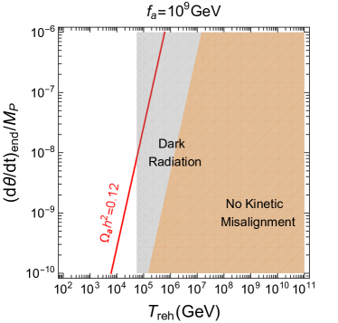
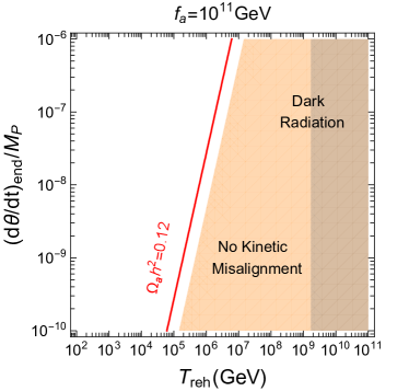
Figure 2: Parameter space in the reheating temperature $T_{\rm reh}$ vs ${\dot{\theta}}_{\rm end}/M_{P}$ for axion dark matter with kinetic misalignment. The correct relic density is obtained by the axion kinetic misalignment along the red line. The kinetic misalignment is sub-dominant in orange regions and the axions produced from the inflaton scattering was in thermal equilibrium, becoming dark radiation. We took $f_{a}=10^{9},10^{11}\,{\rm GeV}$ on the left and right plots, respectively.

For the axion kinetic misalignment to be a dominant mechanism for determining the axion relic density, we obtain the axion relic abundance by

$$\Omega_{a}h^{2}=0.12\bigg{(}\frac{10^{9}\,{\rm GeV}}{f_{a}}\bigg{)}\bigg{(}\frac{Y_{\theta}}{40}\bigg{)}$$ (106)

where $Y_{\theta}$ is the abundance for the axion given by $Y_{\theta}=\frac{n_{\theta}}{s}$ with $n_{\theta}=f^{2}_{a}{\dot{\theta}}$ being the Noether charge density and $s$ being the entropy density. Here, we used $\frac{\rho_{a}}{s}=Cm_{a}(0)Y_{\theta}$ with $C\simeq 2$ to convert the PQ charge abundance to the relic density [8].

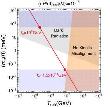
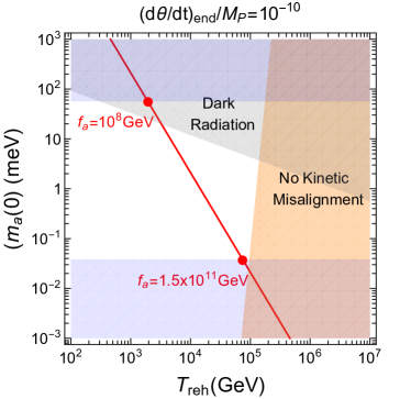
Figure 3: Parameter space in the reheating temperature $T_{\rm reh}$ vs the axion mass $m_{a}(0)$ for axion dark matter with kinetic misalignment. The correct relic density is obtained by the axion kinetic misalignment along the red line. The kinetic misalignment is sub-dominant in orange regions and the axions produced from the inflaton scattering was in thermal equilibrium, becoming dark radiation. We took ${\dot{\theta}}_{\rm end}/M_{P}=10^{-6},10^{-10}$ on the left and right plots, respectively.

In the usual misalignment mechanism, we note that the axion abundance is determined by $Y_{a,{\rm mis}}=\frac{n_{a}}{s}$ at the onset of the axion oscillation at $T=T_{\rm osc}$ [23, 24, 25, 26], namely,

$$Y_{a,{\rm mis}}=0.11\bigg{(}\frac{f_{a}}{10^{9}\,{\rm GeV}}\bigg{)}^{13/6}.$$ (107)

Then, the dominance with the axion kinetic misalignment, namely, $Y_{\theta}>Y_{a,{\rm mis}}$, requires $f_{a}<1.5\times 10^{11}\,{\rm GeV}$ [8].

In Fig. 2, we depict the parameter space for the reheating temperature and the axion velocity at the end of inflation in units of the Planck scale, satisfying the correct relic density by the axion kinetic misalignment in red lines. We show that the axions produced from the saxion scattering becomes thermalized after reheating and provides a detectable dark radiation in gray regions, whereas the kinetic misalignment is sub-dominant in orange regions. The correct relic density is achievable even for a relatively small axion decay constant such as $f_{a}=10^{9}\,{\rm GeV}$ and $10^{11}\,{\rm GeV}$ in the left and right plots, respectively.

In Fig. 3, we show the correlation between the reheating temperature and the axion mass at zero temperature, accounting for the correct relic density from the axion kinetic misalignment in red lines. We chose the initial axion velocity at the end of inflation to ${\dot{\theta}}_{\rm end}/M_{P}=10^{-6},10^{-10}$ in the left and right plots, respectively. At the boundaries of the axion masses satisfying the correct relic density, the corresponding axion decay constant is in the range between $f_{a}=10^{8}\,{\rm GeV}$ and $1.5\times 10^{11}\,{\rm GeV}$, and the reheating temperature varies between $T_{\rm reh}=2\times 10^{5}\,{\rm GeV}$ and $10^{7}\,{\rm GeV}$ for ${\dot{\theta}}_{\rm end}/M_{P}=10^{-6}$, and $T_{\rm reh}=2\times 10^{3}\,{\rm GeV}$ and $7\times 10^{4}\,{\rm GeV}$ for ${\dot{\theta}}_{\rm end}/M_{P}=10^{-10}$, respectively. As in Fig. 2, the region with a detectable dark radiation is shown in gray regions and the kinetic misalignment is sub-dominant in orange regions.

6 Conclusions

We have presented a consistent model of the PQ inflation for realizing the kinetic misalignment of the QCD axion. The radial component of the PQ field drives inflation near the pole of the kinetic term in the Einstein frame, leading to a successful prediction for inflationary observables with a small quartic coupling for the PQ field during inflation. The angular component of the PQ field, namely, the QCD axion, receives a nonzero initial velocity during inflation, due to the PQ violating potential.

We performed the analysis of the perturbative reheating in the presence of the couplings of the PQ field to the SM Higgs as well as the extra vector-like quark responsible for PQ anomalies. We found that a sufficiently large reheating temperature is achieved from the decays and scattering processes of the inflaton and the axions produced from the inflation scattering can become dark radiation at a detectable level in the future CMB experiments if they are thermalized. Thus, as the inflaton reaches the minimum of the potential at reheating completion, the approximately conserved Noether charge for the PQ symmetry survives until the time of the axion oscillation, making the axion kinetic misalignment to be a dominant mechanism for axion dark matter.

Taking the PQ violating potential to be sub-dominant during inflation and free from the axion quality problem in the vacuum, we set the maximum value of the axion velocity at the end of inflation and found the consistent parameter space for the axion kinetic misalignment in the reheating temperature, the initial velocity of the axion and the axion decay constant. For the fixed initial velocity of the axion, the larger the axion decay constant, the smaller the maximum reheating temperature for the axion kinetic misalignment. To be consistent with the astrophysical bounds on the axion couplings and the axion kinetic misalignment, we took the axion decay constant between $f_{a}=10^{8}\,{\rm GeV}$ and $1.5\times 10^{11}\,{\rm GeV}$ and showed that the maximum temperature varies between $T_{\rm reh}=7\times 10^{4}\,{\rm GeV}$ and $10^{7}\,{\rm GeV}$.

References

• [1] R. D. Peccei and H. R. Quinn, Phys. Rev. Lett. 38 (1977), 1440-1443 doi:10.1103/PhysRevLett.38.1440
• [2] J. E. Kim, Phys. Rev. Lett.  43 (1979) 103. doi:10.1103/PhysRevLett.43.103 M. A. Shifman, A. I. Vainshtein and V. I. Zakharov, Nucl. Phys. B 166 (1980) 493. doi:10.1016/0550-3213(80)90209-6.
• [3] M. Dine, W. Fischler and M. Srednicki, Phys. Lett.  104B (1981) 199. doi:10.1016/0370-2693(81)90590-6; A. P. Zhitnitskii, Sov. J. Nucl. Phys. 31, 260 (1980).
• [4] J. Preskill, M. B. Wise and F. Wilczek, Phys. Lett. B 120 (1983), 127-132 doi:10.1016/0370-2693(83)90637-8; L. F. Abbott and P. Sikivie, Phys. Lett. B 120 (1983), 133-136 doi:10.1016/0370-2693(83)90638-X; M. Dine and W. Fischler, Phys. Lett. B 120 (1983), 137-141 doi:10.1016/0370-2693(83)90639-1
• [5] E. Masso, F. Rota and G. Zsembinszki, Phys. Rev. D 66 (2002), 023004 doi:10.1103/PhysRevD.66.023004 [arXiv:hep-ph/0203221 [hep-ph]]; P. Graf and F. D. Steffen, Phys. Rev. D 83 (2011), 075011 doi:10.1103/PhysRevD.83.075011 [arXiv:1008.4528 [hep-ph]].
• [6] A. Salvio, A. Strumia and W. Xue, JCAP 01 (2014), 011 doi:10.1088/1475-7516/2014/01/011 [arXiv:1310.6982 [hep-ph]].
• [7] F. D’Eramo, F. Hajkarim and S. Yun, Phys. Rev. Lett. 128 (2022) no.15, 152001 doi:10.1103/PhysRevLett.128.152001 [arXiv:2108.04259 [hep-ph]].
• [8] R. T. Co, L. J. Hall and K. Harigaya, Phys. Rev. Lett. 124 (2020) no.25, 251802 doi:10.1103/PhysRevLett.124.251802 [arXiv:1910.14152 [hep-ph]].
• [9] R. Kallosh, A. Linde and D. Roest, JHEP 11 (2013), 198 doi:10.1007/JHEP11(2013)198 [arXiv:1311.0472 [hep-th]]; R. Kallosh and A. Linde, JCAP 07 (2013), 002 doi:10.1088/1475-7516/2013/07/002 [arXiv:1306.5220 [hep-th]].
• [10] S. Cléry, H. M. Lee and A. G. Menkara, [arXiv:2306.07767 [hep-ph]].
• [11] M. Kamionkowski and J. March-Russell, Phys. Lett. B 282 (1992), 137-141 doi:10.1016/0370-2693(92)90492-M [arXiv:hep-th/9202003 [hep-th]]; S. M. Barr and D. Seckel, Phys. Rev. D 46 (1992), 539-549 doi:10.1103/PhysRevD.46.539
• [12] M. Fairbairn, R. Hogan and D. J. E. Marsh, Phys. Rev. D 91 (2015) no.2, 023509 doi:10.1103/PhysRevD.91.023509 [arXiv:1410.1752 [hep-ph]]; K. Nakayama and M. Takimoto, Phys. Lett. B 748 (2015), 108-112 doi:10.1016/j.physletb.2015.07.001 [arXiv:1505.02119 [hep-ph]].
• [13] G. Ballesteros, J. Redondo, A. Ringwald and C. Tamarit, Phys. Rev. Lett. 118 (2017) no.7, 071802 doi:10.1103/PhysRevLett.118.071802 [arXiv:1608.05414 [hep-ph]].
• [14] G. Ballesteros, J. Redondo, A. Ringwald and C. Tamarit, JCAP 08 (2017), 001 doi:10.1088/1475-7516/2017/08/001 [arXiv:1610.01639 [hep-ph]].
• [15] Y. Akrami et al. [Planck], Astron. Astrophys. 641 (2020), A10 doi:10.1051/0004-6361/201833887 [arXiv:1807.06211 [astro-ph.CO]].
• [16] P. A. R. Ade et al. [BICEP and Keck], Phys. Rev. Lett. 127 (2021) no.15, 151301 doi:10.1103/PhysRevLett.127.151301 [arXiv:2110.00483 [astro-ph.CO]].
• [17] J. J. Bennett, G. Buldgen, M. Drewes and Y. Y. Y. Wong, JCAP 03 (2020), 003 doi:10.1088/1475-7516/2020/03/003 [arXiv:1911.04504 [hep-ph]]; K. Akita and M. Yamaguchi, JCAP 08 (2020), 012 doi:10.1088/1475-7516/2020/08/012 [arXiv:2005.07047 [hep-ph]]; J. J. Bennett, G. Buldgen, P. F. De Salas, M. Drewes, S. Gariazzo, S. Pastor and Y. Y. Y. Wong, JCAP 04 (2021), 073 doi:10.1088/1475-7516/2021/04/073 [arXiv:2012.02726 [hep-ph]].
• [18] N. Aghanim et al. [Planck], Astron. Astrophys. 641 (2020), A6 [erratum: Astron. Astrophys. 652 (2021), C4] doi:10.1051/0004-6361/201833910 [arXiv:1807.06209 [astro-ph.CO]].
• [19] K. N. Abazajian et al. [CMB-S4], [arXiv:1610.02743 [astro-ph.CO]]; K. Abazajian, G. Addison, P. Adshead, Z. Ahmed, S. W. Allen, D. Alonso, M. Alvarez, A. Anderson, K. S. Arnold and C. Baccigalupi, et al. [arXiv:1907.04473 [astro-ph.IM]].
• [20] J. O. Gong and H. M. Lee, JCAP 11 (2011), 040 doi:10.1088/1475-7516/2011/11/040 [arXiv:1105.0073 [hep-ph]].
• [21] M. A. G. Garcia, K. Kaneta, Y. Mambrini and K. A. Olive, JCAP 04 (2021), 012 doi:10.1088/1475-7516/2021/04/012 [arXiv:2012.10756 [hep-ph]].
• [22] M. Gorghetto and G. Villadoro, JHEP 03 (2019), 033 doi:10.1007/JHEP03(2019)033 [arXiv:1812.01008 [hep-ph]].
• [23] K. J. Bae, J. H. Huh and J. E. Kim, JCAP 09 (2008), 005 doi:10.1088/1475-7516/2008/09/005 [arXiv:0806.0497 [hep-ph]].
• [24] O. Wantz and E. P. S. Shellard, Phys. Rev. D 82 (2010), 123508 doi:10.1103/PhysRevD.82.123508 [arXiv:0910.1066 [astro-ph.CO]].
• [25] G. Grilli di Cortona, E. Hardy, J. Pardo Vega and G. Villadoro, JHEP 01 (2016), 034 doi:10.1007/JHEP01(2016)034 [arXiv:1511.02867 [hep-ph]].
• [26] S. Borsanyi, Z. Fodor, J. Guenther, K. H. Kampert, S. D. Katz, T. Kawanai, T. G. Kovacs, S. W. Mages, A. Pasztor and F. Pittler, et al. Nature 539 (2016) no.7627, 69-71 doi:10.1038/nature20115 [arXiv:1606.07494 [hep-lat]].