Confirmation of a Substantial Discrepancy between Radio and UV–IR Measures of the Star Formation Rate Density at $0.2<z<1.3$

Abstract

We present the initial sample of redshifts for 3,839 galaxies in the MeerKAT DEEP2 field—the deepest $\sim$1.4 GHz radio field yet observed. Using a spectrophotometric technique combining coarse optical spectra with broadband photometry, we obtain redshifts with $\sigma_{z}\leq 0.01(1+z)$. The resulting radio luminosity functions between $0.2<z<1.3$ from our sample of 3,839 individual galaxies are in remarkable agreement with those inferred from modeling radio source counts, confirming an excess in radio-based SFRD$(z$) measurements at late times compared to those from the UV–IR. Several sources of systematic error are discussed—with most having the potential of exacerbating the discrepancy—with the conclusion that significant work remains to have confidence in a full accounting of the star formation budget of the universe.

1 Introduction

Since it was first discovered in the 1990s that the comoving star-formation rate density (SFRD) around $z\sim 1$ dwarfs that of today, immense progress has been made in understanding the general shape of SFRD evolution with cosmic time. Collections of SFRD measurements across wide redshift ranges place the peak of star formation activity near $z\sim 2$ and show a decline by a factor of $\sim$10 to present day (see Hopkins & Beacom, 2006; Madau & Dickinson, 2014, for reviews of the topic).

Despite consistent agreement among the UV/optical and infrared (IR) communities on the SFRD through $z\sim 2$, there has been established tension between the SFRD evolution derived at shorter wavelengths (e.g. UV and optical) with that derived at longer wavelengths (e.g. radio and sub-millimeter). Studies with ALMA have shown that UV measurements of the SFRD miss the obscured, dusty, and heavily star-forming galaxies more common in the distant universe (e.g. Casey et al., 2018; Bouwens et al., 2020). Even in the more “recent” past, Whitaker et al. (2017) found that $>80\%$ of star formation is obscured at all redshifts $z<2.5$ in galaxies having stellar masses $\log[M_{*}/M_{\odot}]\geq 10$. FIR/sub-mm observations are essential to understand dusty galaxies, but single-dish telescopes are only sensitive to the massive, tip-of-the-iceberg sources. Sub-mm interferometers such as ALMA are limited to a very small field-of-view, making it expensive and impractical to amass a deep sample over a large enough area to minimize cosmic variance.

Radio observations are immune to dust obscuration, insensitive to contamination by older stellar populations, and available across wide sky areas. While active galactic nuclei (AGNs) are primarily responsible for powering strong 1.4 GHz radio sources, star-forming galaxies dominate the radio emission below $450\,\mu$Jy (Algera et al., 2020; Matthews et al., 2021a). Star-forming galaxies produce radio emission through two processes: (1) thermal bremsstrahlung from H II regions ionized and heated by massive stars and (2) synchrotron radiation from cosmic-ray electrons accelerated in the shocks of supernova remnants (Condon, 1992).

Synchrotron radiation dominates the radio spectrum at $\nu<10$ GHz. The combined timescale of the massive stars responsible for supernova remnants plus the cooling timescale of cosmic-rays ($\tau_{\mathrm{cool}}<100$ Myr for a spiral galaxy that stopped forming stars after a single episode; Murphy et al., 2008) is small compared to the age of the universe, so the radio emission from star-forming galaxies depends on their current star-formation rates and is uncontaminated by older stellar populations. Although an indirect tracer, the radio luminosity is tightly correlated with the FIR emission from dust heated by massive stars (Helou et al., 1985). This FIR/radio correlation validates the use of radio emission as a quantitative tracer of star-formation in galaxies and has been shown to evolve little to not-at-all through redshift $z\sim 4$ (e.g. Ivison et al., 2010; Magnelli et al., 2015; Pannella et al., 2015).

Unfortunately, galaxies whose radio emission is powered primarily by star-formation are very faint. It is necessary to detect sub-$\mu$Jy sources to account for most of the star formation through $z\sim 1-3$ when galaxies built up the majority of their stellar mass. Using the MeerKAT DEEP2 field—the deepest $\sim$1.4 GHz radio image yet taken—Matthews et al. (2021b) measured brightness-weighted radio source counts $S^{2}n(S)$ down to $0.25\,\mu$Jy. As shown in Condon & Matthews (2018), the brightness-weighted source counts $S^{2}n(S)$ are proportional to the luminosity function integrated over all redshift:

$$S^{2}n(S)=\frac{D_{\mathrm{H_{0}}}}{2\pi\ln(10)}\int_{0}^{\infty}u_{\mathrm{dex}}(L_{\nu}|z)\left[\frac{(1+z)^{\alpha-1}}{E(z)}\right]dz,$$ (1)

where $D_{H_{0}}\equiv c/H_{0}$ is the Hubble distance, $L_{\nu}=4\pi D_{\mathrm{C}}^{2}(1+z)^{1-\alpha}S$ is the luminosity per unit frequency, $D_{\mathrm{C}}$ is the comoving distance, $E(z)=[\Omega_{\mathrm{m}}(1+z)^{3}+\Omega_{\Lambda}+\Omega_{\mathrm{r}}(1+z)^{4}]^{1/2}$, and

$$u_{\mathrm{dex}}(L_{\nu}|z)\equiv L_{\nu}\rho_{\mathrm{dex}}(L_{\nu}|z)=L_{\nu}g(z)\rho_{\mathrm{dex}}\left[\frac{L_{\nu}}{f(z)}|0\right],$$ (2)

where $g(z)$ and $f(z)$ represent density and luminosity evolution, respectively.

Matthews et al. (2021a) determined the evolutionary functions $f(z)$ and $g(z)$ such that the local luminosity function $\rho_{\mathrm{dex}}(L_{\nu}|0)$ evolved backwards matches the observed source counts. At any redshift $z$, the SFRD is proportional to the product $f(z)g(z)$ through the FIR/radio correlation. In this way, Matthews et al. (2021a) constrained the star formation history of the universe for a global population (i.e. there was no information on individual galaxies) by modeling the source counts. The resulting SFRD evolution measured from the deep MeerKAT radio observations is not only stronger than UV/optical measurements, but also stronger than combined UV–IR measurements across all redshifts—deepening the divide between longer and shorter wavelength pictures of the star formation history of the universe.

Recent catalogs of radio continuum sources have been used to probe the SFRD and also found an increase over the UV–IR measurements (e.g. Leslie et al., 2020; Enia et al., 2022; Cochrane et al., 2023). These studies demonstrate many of the difficulties in using radio continuum to trace star formation across redshift: stacking to reach the necessary flux density sensitivity to detect star-forming galaxies (SFGs), relying on photometric redshifts to derive luminosity functions and galaxy characteristics, and observing at lower frequencies where the relationship between radio luminosity and SFR is less understood.

This work introduces a comprehensive multiwavelength follow-up campaign of the MeerKAT DEEP2 field. By surveying the same field whose source counts implied stronger SFR evolution than UV–IR measurements we minimize systematics and robustly test the evolutionary models of Matthews et al. (2021a). Precise redshifts from fitting a combination of low-resolution spectra and optical/NIR photometry of 3,839 galaxies with corresponding MeerKAT detections confirm the cosmic radio SFRD modeling from the source counts and its discrepancy with the UV–IR picture. The results presented here establish a rich framework for dust-unbiased tests of SFR evolution and its diagnostics down to faint, normal galaxies responsible for amassing most of the stellar mass in the universe.

This paper is organized as follows. Section 2 details the multiwavelength, spectrophotometric data of the MeerKAT DEEP2 field. Redshifts are derived from a novel SED fitting technique described in Section 3. We calculate radio luminosity functions from $0.2<z<1.3$ and compare them with models in Section 4. We discuss the implications of confirming radio-based models of stronger SFRD evolution in Section 5.

Absolute quantities were calculated for the flat $\Lambda$CDM universe with $H_{0}=70\,\mathrm{km\,s^{-1}\,Mpc^{-1}}$ and $\Omega_{m}=0.3$. Our spectral-index sign convention is $\alpha\equiv+d\ln\,S/d\ln\,\nu$.

2 Multiwavelength observations of the MeerKAT DEEP2 field

The MeerKAT DEEP2 field was taken as part of commissioning the MeerKAT array (Mauch et al., 2020). The field covers a $\Theta=69.2^{\prime}$ diameter half-power circle centered on J2000 $\alpha=04$:13:26.4, $\delta=-$80:00:00 with a $\theta_{\mathrm{1/2}}=7\farcs 6$ circular Gaussian synthesized beam. The location of the field was optimized to avoid bright radio sources whose large flux densities—combined with systematic position and gain uncertainties of the telescope—limit the achievable dynamic range. About 160 hours of integration resulted in a final thermal noise of $\sigma_{n}=0.56\pm 0.01\,\mu\mathrm{Jy\,beam}^{-1}$. The wideband DEEP2 image is the average of 14 narrow subband images weighted to maximize the signal-to-noise (S/N) of sources with spectral index $\alpha=-0.7$, resulting in an effective frequency of $\nu=1.266\,$GHz. The confusion distribution of faint sources has such a long tail that it is not well-described by its rms. Using the traditional definition of the confusion limit as the flux density at which there are $\gtrsim$25 beam solid angles per source, the “rms” confusion noise is $\sigma_{\mathrm{c}}\approx 2.6\,\mu\mathrm{Jy\,beam^{-1}}$.

Obtaining redshifts for thousands of galaxies typically implies a photometric redshift approach; model or empirical template SEDs are fit to fluxes in broadband filters to determine the physical properties of galaxies. With an effective spectral resolution of $R<10$, current and near-future large imaging surveys achieve uncertainties of at best $\sigma_{z}\gtrsim 0.025(1+z)$ (see Newman & Gruen, 2022, for a review of the topic).

A spectrophotometric approach adds low-resolution ($R\sim 30$) optical prism spectra—which can be obtained for thousands of galaxies in one observation—to the fluxes in broadband filters. The continuous wavelength coverage in the optical with broadband filters extending into the NIR enable redshift uncertainties $\sigma_{z}\leq 0.01(1+z)$ (e.g. Kelson et al., 2014). We adopt this spectrophotometric approach needed to accurately characterize the $\sim$17,000 galaxies in our radio-selected sample. This paper presents initial results from a suite of photometric and spectroscopic observations of the MeerKAT DEEP2 field from the optical through near-infrared. A detailed account of the multiwavelenth observations and a corresponding catalog will be available in Matthews et al. 2024 (in prep). Below is a brief summary of the multiwavelength components contributing to the initial results presented here.

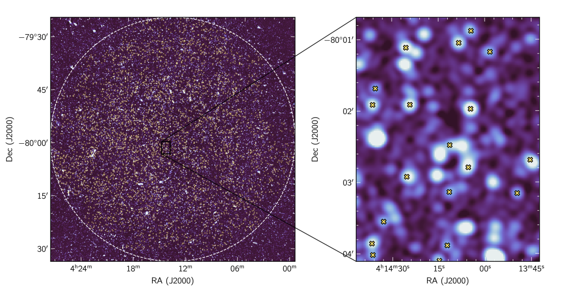
Figure 1: The 1.266 GHz MeerKAT DEEP2 field is shown here—uncorrected for primary beam attenuation—with the half-power point of the primary beam designated as the white dashed circle. Positions of the radio galaxies targeted for optical prism spectra are shown as yellow crosses. The right panel shows an enlarged version of a central $\sim 3\farcm 4\times\sim 2\farcm 6$ region. The initial data release of 3,839 redshifts represents a small fraction of the total radio sources.

2.1 Optical Prism Spectroscopy

The Uniform Dispersion Prism (UDP) on the Inamori Magellan Areal Camera and Spectrograph (IMACS) at Las Campanas Observatory produces low-resolution spectra ($R=\lambda/\Delta\lambda\sim 30$) from 4000–9500 Å. The continuous wavelength coverage through the optical regime yields spectrophotometric redshifts with $\sigma_{z}\leq 0.01(1+z)$ and is key for isolating Balmer breaks and emission lines in star-forming galaxies. Because these spectra span only 150 pixels on the detector, between 1000–2000 objects can be simultaneously observed.

Fourteen pointings of the IMACS f/2 camera with the UDP covered all of the MeerKAT DEEP2 half-power circle (the dashed line in Figure 1). Each of the fourteen masks contained between 1,100 and 1,500 objects, with several objects duplicated between masks of overlapping regions. In total, 11,671 unique radio sources were observed and are identified with yellow crosses in 1. The median exposure time of the final sample is 12,560 seconds with a minimum exposure time of 4,000 seconds and 95% of the objects having exposure times greater than 7,200 seconds.

To guarantee that most of the slits placed on radio sources returned optical spectra, the initial round of objects (the first 7/14 masks) were chosen from the subset of the Matthews et al. (2021b) MeerKAT DEEP2 radio source catalog that had Spitzer cross-identifications within $1^{\prime\prime}$. This criterion applied for all of the first 7/14 masks and 2/3 of the objects on the last 7/14 masks. For the remaining 1/3 of objects on the last 7/14 masks, we relaxed the criterion to include a random selection from a preliminary “deblended” radio catalog made using the XID+ algorithm by Hurley et al. (2017). Since these objects make up $\leq 15\%$ of the targets (and an even smaller fraction of the reduced spectra) details of the deblending and cross-identifications will be described in a future work.

Observations were taken across 8.5 nights spanning February 2022 through January 2023. Typical exposure times for each mask ranged between 160 and 210 minutes.

2.2 Ground-based Optical and Near-Infrared Photometry

As part of programs 2022A-771331 and 2022B-132648, the MeerKAT DEEP2 field was observed by the Dark Energy Camera (DECam) in filters $ugrizY$. Observations spanned 3.5 nights from February 2022 through December 2022. We used the DECam Community Pipeline stacked image product for photometric measurements (Valdes et al., 2014).

Poor atmospheric conditions persisted through most of the observations and limited the resulting seeing FWHM to $\gtrsim 1.2^{\prime\prime}$ in all but $i$ band (where it reached an average seeing of $\sim$0.9^′′). This significantly degraded the achieved depth of the images, resulting in $\sim$5$\sigma$ limiting AB magnitudes of 24.5, 25, 24.75, 24.5, 24.0, and 23.0 for $ugrizY$, respectively.

FourStar is a near-infrared (1–2.5 $\mu$m) camera on the Magellan Baade telescope at Las Campanas Observatory (Persson et al., 2013). It has a field-of-view of $10.8^{\prime}\times 10.8^{\prime}$ composed of four $2048\times 2048$ pixel detectors with a 19^′′ gap in between them. Covering the $\sim$1.1 deg² MeerKAT DEEP2 field required a tiling pattern of 36 FourStar footprints.

Observations were taken in the $J$-band filter (1.1–1.4 $\mu$m) over 2.5 nights from February 2022 through December 2023. The average seeing over multiple nights of observation was $1\farcs 1$. Each pointing was dithered 9 times in a square pattern around the central position with dither offsets of 26^′′ to cover the 19^′′ gap between the detectors. Data reduction and image processing was done using the custom pipeline FourCLift developed and described in Kelson et al. (2014).

2.3 Warm-Spitzer 3.6 $\mu$m and 4.5 $\mu$m imaging

The observations were carried out in twelve distinct epochs (Astronomical Observation Requests or AORs) from 8 July 2019 through 11 December 2019 and totaled 69.4 hours (Spitzer PID:14246). Each AOR consisted of a 14$\times$14 mosaic of 100 s frames, using a single point from the cycling dither pattern to break up the mosaic grid pattern. We included small ($\sim 10^{\prime\prime}$) offsets in the central position, and, because the field is close to the southern continuous viewing zone (CVZ), there was a spread in position angle of the individual mosaics. All together, this ensured full coverage of the circular field containing the FWHM of the MeerKAT primary beam sensitivity (although, sources can be detected beyond this). The reduction of the IRAC photometry was completed in the standard way using the MOPEX data reduction package (Makovoz & Khan, 2005).

2.4 Photometric Measurements

All astrometry was registered to Gaia DR3. Our deepest optical data was taken in the DECam $i$ filter, so we used this image to detect optical counterparts in the MeerKAT DEEP2 field. We used Source Extractor to calculate and subtract the background and subsequently detect sources using the default parameters. We ran aperture photometry on the resulting $\sim 10^{6}$ detections with a $4^{\prime\prime}$ diameter aperture to ensure all source flux of galaxies at intermediate redshifts and beyond is encompassed. The magnitude zeropoints in $grizYJ$ were simultaneously fit to match the synthesized stellar locus according to the algorithms in Kelly et al. (2014). The $u$-band zeropoint was then calibrated using the “blue tip” of halo stars as described in Liang & von der Linden (2023).

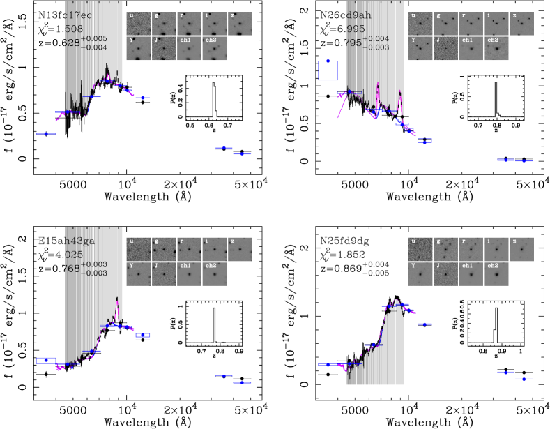
Figure 2: Four examples of radio galaxy SEDs are shown with their multiwavelength photometry and redshift probability distribution. Observed spectra and photometric flux values are shown in black. Our best-fitting model spectra and predicted photometric flux values are shown as the magenta line and blue points, respectively.

3 An eigenvector approach to SED modeling

Constraining galaxy evolution necessitates accurate physical parameters from SED fitting. The accuracy and complexity can come at the expense of longer computation times, particularly for large samples of thousands of galaxies. We developed a new algorithm for SED fitting based upon the fact that SEDs can be constructed from a linear combination of basis functions. The details of this method will be fully described in Kelson et al. (in prep). In summary, we choose to abandon the idea that each basis function has a physical meaning and rather utilize the basis functions as eigenvectors that can be combined in various magnitudes to match a wide variety of galaxy SEDs.

3.1 Construction of Eigenvectors

Each point in the redshift-metallicity-reddening grid has 100,000 star-formation histories generated stochastically via the method introduced in Kelson (2014). We first establish a grid of redshift, metallicity, and reddening values. There are 501 redshifts at intervals of $\log\,z=0.005$ between $-2\leq\log\,z\leq 0.5$, six metallicity values spaced at 0.3 dex intervals from -1.2 to 0.3, and eleven increments of $\log\,A_{\mathrm{V}}$ spaced at 0.25 dex intervals between $-2\leq\log\,A_{\mathrm{V}}\leq 0.5$. We adopt the reddening law of Cardelli et al. (1989), which gave the best results (on average). In future iterations of this novel fitting method, we will be incorporating finer increments in metallicity and reddening, and exploring variation in the reddening law.

Singular value decomposition (SVD) of the resulting galaxy SEDs produces a plethora of basis functions, but many fall below observational noise and are discarded (for example, the signal-to-noise of the present sample requires three to six). To capture the diversty of stellar populations to a part in a thousand requires 9 eigenvectors. The spectroscopy—and photometry—here, like most survey data, are not accurate to a part in a thousand with a full accounting of flux calibration and photometric uncertainties, allowing us to restrict the fits to fewer basis functions without any loss of information.

3.2 Data Fitting

We obtained IMACS-UDP spectra for 11,671 unique sources. Of these, 9,611 had corresponding photometry in the DECam filters $ugrizY$ and remained candidates for SED fitting (which requires $\geq$3 number of photometric measurements in the optical).

Every observed galaxy SED is fit using a linear superposition of up to $N\leq 9$ eigenvectors plus five nonnegative emission line vectors. The maximum number of eigenvectors $N$ per galaxy is determined when the reduced $\chi^{2}$ is no longer improved by adding more eigenvectors. The superposition of eigenvectors accurately recreates the full diversity of galaxy stellar populations and we include the following five (non-negative, Gaussian) emission lines in order to capture the full diversity of galaxy SEDs (see, e.g., Fig. 2): $H\alpha$, N II, O III (a superposition of 5007Å and 4959Å in the ratio 3:1), $H\beta$, the O II doublet at 3727Å (treated as two equal-magnitude Gaussians separated by 2.7 Å in the restframe), and Mg 2959Å.

The final number of source SEDs successfully fit using our novel eigenvector approach is 9,416. Four sources are shown for context in Figure 2. We are encouraged by the strong combination of efficiency and accuracy using this method. To arrive at our final sample, we cut interloping stars from our Galaxy and outliers indicating poor data quality, using a broad and strict range of metrics–both spectroscopic and photometric.

4 Radio source evolution

Comparisons of the space densities of galaxies as functions of luminosity (i.e. luminosity functions) at different points in time trace cosmological evolution. Models correctly describing this evolution thus constrain the buildup of stellar mass over cosmic time. Below, we describe the completeness of our sample—in both radio (Section 4.1) and optical (Section 4.2)—and the corrections we made to overcome inevitable incompleteness. Finally, in Section 4.3 we recount our luminosity function derivation and discuss the effects (or lack thereof) due to cosmic variance (Section 4.4).

4.1 Radio Reliability and Completeness

The sensitivity of the MeerKAT DEEP2 image is limited by point-source confusion (rms $\sigma_{c}\sim 2.6\,\mu$Jy everywhere), not by noise (rms $\sigma_{n}=0.56\,\mu$Jy at the pointing center increasing to $1.12\,\mu$Jy at the primary beam half-power circle). Catalogs of individual sources fainter than $S\sim 10\,\mu\mathrm{Jy}\sim 4\sigma_{c}$ become increasingly incomplete and unreliable. In the case of MeerKAT DEEP2, the catalog was cut off at $S_{\mathrm{1.266\,GHz}}=10\,\mu\mathrm{Jy}$ ($\sim$18$\sigma_{n}$) to ensure high completeness and reliability as determined through injecting sources into mock images (Matthews et al., 2021b). Because the limiting flux density of the radio source catalog is independent of the thermal noise, the catalog sensitivity and completeness is uniform across the image. This translates to exceedingly simple radio completeness corrections that depend on flux density alone.

Ten mock images of the MeerKAT DEEP2 field were created by Matthews et al. (2021b) and cataloged with the same source finding algorithm employed on the real data. The completeness of the real source catalog was determined by comparing the number of input sources into the mock images with the number cataloged by the source finding algorithm. The catalog at the faint limit of $S_{\mathrm{1.266\,GHz}}=10\,\mu\mathrm{Jy}$ is 57% complete and quickly jumps to $\gtrsim 96\%$ complete by $S_{\mathrm{1.266\,GHz}}=20\,\mu\mathrm{Jy}$.

These same ten mock images were used to estimate the reliability $0\leq R\leq 1$ at the faint end of radio catalog. We estimated the reliability as a function of flux density $S$ by determining the fraction of sources with measured flux densities within $0.5\,\mu$Jy of $S=10.5,11.5,12.5,13.5,14.5$, and 15.5$\,\mu$Jy whose true flux densities actually lie $3\sigma_{n}$ below the sample limit of $S=10\,\mu$Jy. The reliability in the intervals $[10\,\mu\mathrm{Jy},11\,\mu\mathrm{Jy})$, $[11\,\mu\mathrm{Jy},12\,\mu\mathrm{Jy})$, $[12\,\mu\mathrm{Jy},13\,\mu\mathrm{Jy})$, $[13\,\mu\mathrm{Jy},14\,\mu\mathrm{Jy})$, and $[14\,\mu\mathrm{Jy},15\,\mu\mathrm{Jy})$ is 0.84, 0.90, 0.95, 0.97, and 0.99, respectively.

4.2 Optical Completeness

The poor seeing prevented our DECam observations from reaching the intended $i=25$ magnitude limit. Nonetheless, because the seeing and depth of the $i$-band data are superior to the other bands, we use it to define the positions of galaxies associated with the radio detections for the photometry behind the SEDs. Cross-identifying optical counterparts in the $i$ band image yields 14,679 matches within $2.5^{\prime\prime}$ (smaller than half the FWHM of the MeerKAT-DEEP2 beam) of the 17,150 radio galaxies.

The fraction of these 14,679 galaxies with successful SED fitting represents the optical completeness of the radio sample. 3,839 galaxies had both successful IMACS spectra extraction, high enough S/N, sufficient data quality and fidelity, and enough photometric bands to fit an SED with high accuracy. We partitioned the 14,679 galaxies into $\log S$ bins of width 0.2 from $\log[S\,(\mathrm{Jy})]=-5$ to $\log[S\,(\mathrm{Jy})]=-2$. For each bin, the completeness is defined as the ratio of the number of galaxies with a successful SED fit to the total number within each bin. We are most complete ($\sim$44%) at a $i=21$ and the completeness falls near-linearly to $\sim$5% at $i=24$. We limit our luminosity function calculations to $i=23.5$, the point at which the completeness falls to $12.5\%$, just over a quarter of its peak value.

4.3 Radio luminosity functions

We calculate luminosity functions in several contiguous redshift slices using the 1/$V_{\mathrm{max}}$ method (Schmidt, 1968). Redshift bins were defined to be only wide enough such that the Poisson counting errors in a redshift slice are at most $\sim 5\%$ ($N\approx 350$). Redshift slices that are narrow serve to mitigate against the impact of evolving stellar populations, whereby some galaxies that may have sufficient photometry at the front end of a slice would have had photometric properties—owing to both mass growth and stellar evolution—at the backside of the redshift slice that leave them excluded by the DECam imaging depth. These effects complicate the estimation of $V_{\mathrm{max}}$. By narrowing the redshift slices, we keep this source of systematic uncertainty to less than 10%.

The maximum comoving volume over which a galaxy can be observed $V_{\mathrm{max}}=V(z_{\mathrm{max}})-V(z_{\mathrm{min}})$ is the volume of the redshift bin over which the source is observable. It is bounded on one side by $z_{\mathrm{min}}$, the lower bound of the redshift bin containing the galaxy. On the high end, the maximum redshift $z_{\mathrm{max}}$ is the minimum of the following: (1) the redshift at which the galaxy falls out of the radio sample ($S_{\mathrm{1.266\,GHz}}<10\,\mu$Jy), (2) the redshift at which the galaxy falls out of the optical sample ($i>23.5$—and assuming a galaxy’s color does not evolve over the time span of its respective redshift slice), or (3) the maximum redshift of the redshift slice containing the galaxy.

The spectral luminosity $L_{\mathrm{1.4\,GHz}}$ at redshift $z$ depends on the observed flux density of the source and the spectral index of the source population

$$L_{\mathrm{1.4\,GHz}}(z)=4\pi D_{L}^{2}(1+z)^{-\alpha-1}\left(\frac{1.4}{1.266}\right)^{\alpha}S_{\mathrm{1.266\,GHz}},$$ (3)

where we assume the standard $\alpha=-0.7$ for radio populations at $\sim$1.4 GHz.

Unlike in the radio regime, the SED of a galaxy in the optical does not follow a power law and depends sensitively on the K-correction.

$$m_{i}(z)=M_{i}+\mathrm{DM}(z)+K_{i}(z),$$ (4)

where $m_{i}$ is the apparent magnitude of the source at redshift $z$, $M_{i}$ is the $i$ band absolute magnitude, DM$(z)$ is the distance modulus, and $K_{i}(z)$ is the K-correction at $i$ band. We modeled the K-correction using the kcorrect software by Blanton & Roweis (2007). We assume the galaxy SED—the best-fit spectral template from kcorrect—does not change within its redshift bin and calculate the maximum redshift for which $m_{i}\leq 23.5$.

For each luminosity bin, the space density of radio sources is calculated by the following:

$$\rho_{\mathrm{dex}}(L,z)=\frac{1}{\Delta\log\,L}\sum_{i=1}^{N}\left[c_{i}\,V_{\mathrm{max},i}\right]^{-1},$$ (5)

where $\Delta\log\,L$ is the width of the luminosity bin, $V_{\mathrm{max},i}$ is the maximum comoving volume over which the $i$th galaxy could be observed,

$$V_{\mathrm{max,i}}=\frac{\Omega}{4\pi}[V(z_{\mathrm{max,i}})-V(z_{\mathrm{min,i}})],$$ (6)

where $\Omega$ is the survey area in steradians, and $c_{i}$ is the completeness correction factor for the $i$th galaxy. Luminosity bins are of width 0.2 dex centered on $\log[L_{\mathrm{1.4\,GHz}}(\mathrm{W\,Hz^{-1}})]=21.1,21.3,\ldots,25.3$.

The scenario in which our sample is 100% complete—where we have measured redshifts for every radio source at $z<1.3$ and that all other sources are at $z>1.3$—is illustrated by the open circles in Figure 3. Assuming all unmeasured objects are at $z<1.3$ leads to luminosity functions that are significantly higher than the model predictions. Here, we presume completeness corrections assuming that the true fraction of radio sources at $z<1.3$ is that implied by the modeling from Matthews et al. (2021a). The completeness correction factor $c_{i}$ for the $i$th galaxy includes a term for the reliability of the radio catalog as a function of flux density $R_{\mathrm{r}}(S)$, for the completeness of the radio survey as a function of flux density $C_{\mathrm{r}}(S)$, for the optical/redshift completeness of the radio sample as a function of flux density $C_{\mathrm{opt}}(S)$, and for the fraction of objects at flux density $S$ that lie within $z<1.3$ by the evolutionary models of Matthews et al. (2021a). The final completeness correction factor for the $i$th galaxy is as follows:

$$c_{i}=\frac{R_{\mathrm{r}}(S)\,f_{z<1.3}(S)}{C_{\mathrm{r}}(S)\,C_{\mathrm{opt}}(S)}.$$ (7)

The errors are the quadrature sum of the expected fractional cosmic variance and rms Poisson counting errors for independent galaxies. If the number of galaxies in a luminosity bins is small ($N<5$), the counting errors are taken from the 84% confidence limits tabulated in Gehrels (1986). The uncertainty caused by cosmic variance is described below in Section 4.4.

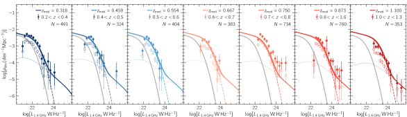
Figure 3: Radio luminosity functions in increasing redshift slices with the median redshift displayed in the top right corner of each panel. Filled circles represent measured number densities of radio sources—corrected for both radio and optical incompleteness—as a function of spectral radio luminosity. Open circles represent the number densities of the same sample without completeness corrections. All error bars reflect $1\sigma$ uncertainties. Solid colored line: radio luminosity functions predicted by Matthews et al. (2021a) for galaxies (both star-forming and AGN) at the median redshift of the galaxies in each redshift bin. Dashed colored line: predicted radio luminosity of star-forming galaxies at the median redshift. Dotted colored line: predicted radio luminosity of AGNs at the median redshift. Thick gray line: local radio luminosity function of star-forming galaxies from Condon et al. (2019).

4.4 Cosmic Variance

We estimated cosmic variance using the tools of Trenti & Stiavelli (2008). Because this method relies on halo clustering to underpin its calculations, we needed to crudely estimate the range of halo masses that our radio sources reside in. We used the average stellar masses determined via SED fitting in conjunction with the stellar-to-halo mass relation presented in Leauthaud et al. (2012) to estimate the average halo mass $M_{\mathrm{200b}}$, where $M_{\mathrm{200b}}$ is defined as the mass within the radius at which the mean interior density is equal to 200 times the mean matter density.

Based on the estimated average halo masses, we used the Cosmic Variance Calculator to estimate the fractional cosmic variance in each redshift bin (Trenti & Stiavelli, 2008). In addition to the 1–$\sigma$ uncertainty on the number counts and other sample statistics, the Cosmic Variance Calculator outputs the minimum mass of dark matter halos hosting galaxies in the sample. In each redshift bin, we adjusted the intrinsic number of objects the survey is expected to observe until the minimum halo mass agrees with the average halo mass determined from the Leauthaud et al. (2012) stellar-to-halo mass relation.

Ultimately, the fractional count error due to cosmic variance is consistently less than 0.16 across all redshift slices in our sample. Tweaking the parameters used in the Cosmic Variance Calculator had little effect on the output cosmic variance values and therefore inconsequential effects on the space densities of radio galaxies determined in this work. The error bars shown in Figure 3 include the conservative cosmic variance uncertainty added in quadrature with Poisson counting errors.

4.5 Estimating radio-based SFRD($z$)

Converting radio luminosities to SFRs deserves extensive care and a thorough investigation of possibly uncertainties (as will be outlined in Section 5). However, to guide such discussion and quantify the possible disagreement in the SFRD($z$) between radio and UV–IR studies, we present an initial conversion between the calculated radio luminosity functions and SFRD$(z)$.

The SFRD at any redshift $z$ is related to the total radio energy density produced by star-forming galaxies. In each redshift slice, we fit the projected luminosity-weighted luminosity functions (e.g. energy density functions) of SFGs and AGNs combined to the observed data. As an initial estimate, we assume the form of the luminosity functions modeled by Matthews et al. (2021a) and only allow a renormalization of the SFG energy density function with respect to both axes (i.e. a scale and a shift).

To properly compare the observed SFRD in each redshift slice with that predicted by the Matthews et al. (2021a) evolutionary models, we adopt their prescription to convert radio luminosity to SFR. In short, we assume the relationship between SFR and integrated IR luminosity ($8<\lambda(\mu\mathrm{m})<1000$) of Murphy et al. (2011) with the average ratio between total IR luminosity and FIR luminosity ($42.5<\lambda(\mu\mathrm{m})<122.5$) measured by Bell et al. (2003). The radio estimate of the SFRD for a Kroupa (2001) IMF at any time $t$ is

$$\left[\frac{\psi(t)}{M_{\odot}\,\mathrm{yr^{-1}\,Mpc^{-3}}}\right]=7.39\times 10^{-37}\cdot 3.75\times 10^{12}\,\mathrm{Hz}$$ (8)

$$\cdot\int\left[\frac{u_{\mathrm{dex}}(L_{\nu}|t)\cdot 10^{\langle q(L_{\nu})\rangle}}{\mathrm{W\,Hz^{-1}\,Mpc^{-3}}}\right]d\log(L_{\nu}),$$

where $\langle q(L_{\nu})\rangle$ is the ratio of the FIR and radio luminosities from Matthews et al. (2021a):

$$\langle q\rangle =2.69-0.147[\log(L_{\nu})-19.1]\ \mathrm{if\ \log(L_{\nu})<22.5}$$

$$\langle q\rangle =2.19\ \mathrm{if\ \log(L_{\nu})}\geq 22.5.$$ (9)

We adopt conservative integration limits for our evaluations of Equation 8. Our lower integration limits are set to $L_{*}/4$, where $L_{*}$ is determined by evolving the local value $L_{*}(z=0)=1.9\times 10^{21}\,\mathrm{W\,Hz^{-1}}$ according to the luminosity evolution model from Matthews et al. (2021a). From the local energy density function, setting this as the lower limit potentially misses $\sim$12% of the total SFRD. Nonetheless, using $L_{*}/4$ as the lower luminosity limit for the integration minimizes uncertainties in the SFRD due to possible changes in the faint-end slope of the luminosity function.

We adopt an upper integration limit of $\log[L_{\mathrm{1.4\,GHz}}\,(\mathrm{W\,Hz^{-1}})]=24$. Although we detect radio sources above this luminosity, the highest luminosity bins are the most likely to be contaminated by AGNs and therefore contribute disproportionately to the estimated SFRD. Adopting this upper integration limit minimizes the possibility that AGN contamination can explain a radio SFRD that is enhanced compared with UV–IR measurements.

Figure 4 shows our conservative, radio-based SFRD measurements at the median redshift of each redshift slice. Further work to (1) push to fainter flux densities (and therefore further down the faint end of the luminosity function) and (2) carefully separate SFGs and AGNs in the MeerKAT DEEP2 sample will expand the integration limits and place stronger constraints on the radio-SFRD($z$).

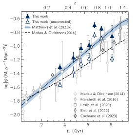
Figure 4: The SFRD from present day to a lookback time of $t_{L}=9.5$ Gyr. A sample of UV–IR (Madau & Dickinson, 2014; Marchetti et al., 2016) and recent radio (Leslie et al., 2020; Enia et al., 2022; Cochrane et al., 2023) continuum SFRD measurements are shown for comparison. SFRD measurements from 3,839 galaxies in the MeerKAT DEEP2 field are shown as filled, thick triangles. Unfilled thin diamonds show the SFRD measurements from the MeerKAT DEEP2 sample without any corrections for sample incompleteness.

5 Potential sources of discrepancy in the SFRD evolution and Implications

At the end of the previous section, we showed star formation rate densities—inferred from our luminosity functions—in Figure 4. These SFRDs—shown by the filled, dark triangles—are compared to those from other radio studies (e.g. Leslie et al., 2020; Enia et al., 2022; Cochrane et al., 2023), and to a sampling of UV–IR estimates. While this study advances our understanding of the radio-SFRD by coupling the deepest radio image with a large spectrophotometric sample, the tension with UV–IR measurements has been seen across multiple radio studies (such as those listed above). Given that the luminosity functions agreed with those predicted by Matthews et al. (2021a), Figure 4 also shows that our SFRD measurements agree with the SFRD evolution of the Matthews et al. (2021a) modeling.

The radio values for SFRD between $(0.2\leq z\leq 1.3)$ are 50% to 100% higher than canonical estimates from not only UV/optical, but also, seemingly, over combined UV–IR measurements. This discrepancy suggests more than a mild tension, but rather a fundamental disagreement, in one of the most important metrics for understanding the evolution of our Universe. Here we discuss sources of systematic uncertainty, quantify their impact on SFRD calculations, and explore possible reasons for disagreement between radio and UV–IR based SFRD$(z)$.

5.1 Budget of systematic uncertainties

A full budget of systematic uncertainties must include many potential issues, some of which have been mentioned already. In Section 4.4 the uncertainty due to cosmic variance was estimated to be $\sim$15% (0.06 dex). Other potential sources of uncertainty include confusion effects, completeness correction factors, contamination by AGN, and the FIR/radio correlation parameter $q$.

The volume surveyed here, and the modest beam size, are both large enough to produce more than zero incidents of coincidence between galaxies and background radio sources along the line of sight. We generated mock MeerKAT images and catalogs using the model radio luminosity functions of Matthews et al. (2021a), simulating the observed luminosity functions and the effects of object coincidence. At $z<0.7$ and $z>1$ the effect is negligible, while at $0.7<z<0.9$ the observed luminosity functions may be contaminated by line of sight superposition at a level that can, on average, skew the luminosities of sources by $+0.05$ dex.

There is an additional systematic uncertainty that arises from the modeling of spectroscopic incompleteness, as having only securely measured redshifts for a fraction of the radio catalog. We estimate this uncertainty by summing the galaxy weights in our final catalog of $3,839$ galaxies and comparing to the size of what ought to be the parent catalog—the number of radio galaxies in the MeerKAT DEEP2 catalog multiplied by the fraction of those expected to have $z<1.3$. This latter term is model dependent and we adopt a flux-density dependent fraction from Matthews et al. (2021a). We find the sum of galaxy weights (i.e. inverse completeness) to be within $\sim 10\%$ of the size of our parent catalog. As such, we estimate errors in the completeness correction factor to add $\sim$10% uncertainty (0.04 dex) to our SFRD measurements.

The fraction of AGN in our radio sample will decrease with decreasing flux density. Further, since AGN components are omitted in our SED fitting method, AGN exhibiting strong spectral features in the optical will result in poor SED fits and are therefore cut from our sample following our conservative data quality criteria. Nonetheless, radio emission powered by AGN is present in our sample at some level. After identifying AGN with a wide variety of multiwavelength diagnostics, Algera et al. (2020) found that at $S_{\mathrm{3\,GHz}}=30\,\mu$Jy the fraction of radio sources powered primarily by star-formation reaches $90\%$. At $1.266\,\mathrm{GHz}$, $S_{\mathrm{3\,GHz}}=30\,\mu$Jy equals $\sim 55\,\mu$Jy (assuming $\alpha=-0.7$). While 82% of our sample lie below this flux density value, we conservatively assume 10% of our radio emission is contributed by AGN. As such, AGN contamination add $\sim$0.04 dex to the total error budget on our SFRD measurements.

5.2 Sources of disagreement

Disagreement can arise for two reasons: problems in the measurements (UV, IR, and/or radio) themselves, or problems in the conversions from these measurements to SFRs. This work will focus on areas of improvement for radio-based determinations of the SFRD($z$).

Particularly important to our work is the calibration of radio continuum as a tracer of SFR through the FIR/radio correlation. Conservatively, we have used the sub-linear relation calculated for SFGs in the local universe by Matthews et al. (2021a). Had $\langle q\rangle=2.34\pm 0.01$ been adopted from the seminal work of Yun et al. (2001)—using galaxies in the local universe—our SFRDs would increase further by $\sim$0.1 dex. The SFRD calculated by Leslie et al. (2020) (shown in Figure 4) also adopted a sub-linear IR/radio correlation (Molnár et al., 2021). Molnár et al. (2021) calculated the total-IR (TIR, $8<\lambda(\mu\mathrm{m})<1000$) to radio correlation, but—assuming the conversion between TIR and FIR by Bell et al. (2003)—this relationship yields consistent SFRD measurements when applied to our sample.

When added in quadrature the multiple sources of systematic error in our SFRD measurements yield $\sim 0.1$ dex. Given the combined random and systematic uncertainties, our measurements substantially agree with the model by Matthews et al. (2021a) of SFRD evolution (the redshift slices at $z\sim 0.7-1$ yield SFRD measurements $\sim 2-3\sigma$ high) and in significant disagreement with the SFRD characterized by “canonical” UV–IR estimators. While some sources of systematic errors cannot be mediated (e.g. cosmic variance), others can be improved. Further analysis of the MeerKAT DEEP2 field will explore the connection between radio luminosity and SFR across a wide variety of galaxy stellar masses and SFRs. Comparison of SFRs derived from SED fitting (some of which are supplemented by emission line fluxes measured directly from the spectra) with those by radio luminosity will illuminate areas of galaxy parameter space where these diagnostics disagree. Particular attention to resolving the cause behind these SFR disagreements will inevitably improve our understanding of dust-reddening evolution, cosmic-ray diffusion, and stellar mass buildup in star-forming galaxies.

6 Summary

Along with other radio continuum studies, Matthews et al. (2021a) measured stronger star-formation rate density evolution across all redshifts than what has been measured in the UV–IR. The evolutionary functions by Matthews et al. (2021a) were constrained such that backward-evolving and integrating the local luminosity functions over all redshifts reproduced the observed source counts. As such, these evolutionary functions were derived for a global ensemble and questions remained whether the models could predict the evolution for a sample of individual galaxies with redshift measurements.

We present initial results from the spectrophotometric multiwavelength follow-up of the MeerKAT DEEP2 field. Using a novel SED-fitting method on a combination of low-resolution spectra and optical/NIR photometry, we determined redshifts for 3,839 galaxies spanning $0.2<z<1.3$. The luminosity functions measured from the collection of these individual radio galaxies agrees remarkably well with the luminosity and density evolutionary models derived from only global (i.e. lacking any individual-galaxy level information) radio source counts. Further scrutiny of systematics and a detailed approach to converting radio luminosities to SFRs—and comparing them with other multiwavelength diagnostics—will be presented in a subsequent paper.

References

- Algera et al. (2020) Algera, H. S. B., van der Vlugt, D., Hodge, J. A., et al. 2020, ApJ, 903, 139
- Bell et al. (2003) Bell, E. F., McIntosh, D. H., Katz, N., & Weinberg, M. D. 2003, ApJS, 149, 289
- Blanton & Roweis (2007) Blanton, M. R., & Roweis, S. 2007, AJ, 133, 734
- Bouwens et al. (2020) Bouwens, R., González-López, J., Aravena, M., et al. 2020, ApJ, 902, 112
- Cardelli et al. (1989) Cardelli, J. A., Clayton, G. C., & Mathis, J. S. 1989, ApJ, 345, 245
- Casey et al. (2018) Casey, C. M., Zavala, J. A., Spilker, J., et al. 2018, ApJ, 862, 77
- Cochrane et al. (2023) Cochrane, R. K., Kondapally, R., Best, P. N., et al. 2023, MNRAS, 523, 6082
- Condon (1992) Condon, J. J. 1992, ARA&A, 30, 575
- Condon & Matthews (2018) Condon, J. J., & Matthews, A. M. 2018, PASP, 130, 073001
- Condon et al. (2019) Condon, J. J., Matthews, A. M., & Broderick, J. J. 2019, ApJ, 872, 148
- Enia et al. (2022) Enia, A., Talia, M., Pozzi, F., et al. 2022, ApJ, 927, 204
- Gehrels (1986) Gehrels, N. 1986, ApJ, 303, 336
- Helou et al. (1985) Helou, G., Soifer, B. T., & Rowan-Robinson, M. 1985, ApJ, 298, L7
- Hopkins & Beacom (2006) Hopkins, A. M., & Beacom, J. F. 2006, ApJ, 651, 142
- Hurley et al. (2017) Hurley, P. D., Oliver, S., Betancourt, M., et al. 2017, MNRAS, 464, 885
- Ivison et al. (2010) Ivison, R. J., Magnelli, B., Ibar, E., et al. 2010, A&A, 518, L31
- Kelly et al. (2014) Kelly, P. L., von der Linden, A., Applegate, D. E., et al. 2014, MNRAS, 439, 28
- Kelson (2014) Kelson, D. D. 2014, arXiv e-prints, arXiv:1406.5191
- Kelson et al. (2014) Kelson, D. D., Williams, R. J., Dressler, A., et al. 2014, ApJ, 783, 110
- Kroupa (2001) Kroupa, P. 2001, MNRAS, 322, 231
- Leauthaud et al. (2012) Leauthaud, A., Tinker, J., Bundy, K., et al. 2012, ApJ, 744, 159
- Leslie et al. (2020) Leslie, S. K., Schinnerer, E., Liu, D., et al. 2020, ApJ, 899, 58
- Liang & von der Linden (2023) Liang, S., & von der Linden, A. 2023, MNRAS, 519, 2281
- Madau & Dickinson (2014) Madau, P., & Dickinson, M. 2014, ARA&A, 52, 415
- Magnelli et al. (2015) Magnelli, B., Ivison, R. J., Lutz, D., et al. 2015, A&A, 573, A45
- Makovoz & Khan (2005) Makovoz, D., & Khan, I. 2005, in Astronomical Society of the Pacific Conference Series, Vol. 347, Astronomical Data Analysis Software and Systems XIV, ed. P. Shopbell, M. Britton, & R. Ebert, 81
- Marchetti et al. (2016) Marchetti, L., Vaccari, M., Franceschini, A., et al. 2016, MNRAS, 456, 1999
- Matthews et al. (2021a) Matthews, A. M., Condon, J. J., Cotton, W. D., & Mauch, T. 2021a, ApJ, 914, 126
- Matthews et al. (2021b) —. 2021b, ApJ, 909, 193
- Mauch et al. (2020) Mauch, T., Cotton, W. D., Condon, J. J., et al. 2020, ApJ, 888, 61
- Molnár et al. (2021) Molnár, D. C., Sargent, M. T., Leslie, S., et al. 2021, MNRAS, 504, 118
- Murphy et al. (2008) Murphy, E. J., Helou, G., Kenney, J. D. P., Armus, L., & Braun, R. 2008, ApJ, 678, 828
- Murphy et al. (2011) Murphy, E. J., Condon, J. J., Schinnerer, E., et al. 2011, ApJ, 737, 67
- Newman & Gruen (2022) Newman, J. A., & Gruen, D. 2022, ARA&A, 60, 363
- Pannella et al. (2015) Pannella, M., Elbaz, D., Daddi, E., et al. 2015, ApJ, 807, 141
- Persson et al. (2013) Persson, S. E., Murphy, D. C., Smee, S., et al. 2013, PASP, 125, 654
- Schmidt (1968) Schmidt, M. 1968, ApJ, 151, 393
- Trenti & Stiavelli (2008) Trenti, M., & Stiavelli, M. 2008, ApJ, 676, 767
- Valdes et al. (2014) Valdes, F., Gruendl, R., & DES Project. 2014, in Astronomical Society of the Pacific Conference Series, Vol. 485, Astronomical Data Analysis Software and Systems XXIII, ed. N. Manset & P. Forshay, 379
- Whitaker et al. (2017) Whitaker, K. E., Pope, A., Cybulski, R., et al. 2017, ApJ, 850, 208
- Yun et al. (2001) Yun, M. S., Reddy, N. A., & Condon, J. J. 2001, ApJ, 554, 803