Driving superconducting qubits into chaos

Abstract

Kerr parametric oscillators are potential building blocks for fault-tolerant quantum computers. They can stabilize Kerr-cat qubits, which offer advantages towards the encoding and manipulation of error-protected quantum information. Kerr-cat qubits have been recently realized with the SNAIL transmon superconducting circuit by combining nonlinearities and a squeezing drive. These superconducting qubits can lead to fast gate times due to their access to large anharmonicities. However, we show that when the nonlinearities are large and the drive strong, chaos sets in and melts the qubit away. We provide an equation for the border between regularity and chaos and determine the regime of validity of the Kerr-cat qubit, beyond which it disintegrates. This is done through the quantum analysis of the quasienergies and Floquet states of the driven system, and is complemented with classical tools that include Poincaré sections and Lyapunov exponents. By identifying the danger zone for parametric quantum computation, we uncover another application for driven superconducting circuits, that of devices to investigate quantum chaos.

I Introduction

Decoherence is a familiar threat to quantum technologies. A resourceful way to protect quantum information against decoherence processes that act locally is to encode it nonlocally in the phase space of an oscillator in the form of superpositions of coherent states [1]. These Schrödinger cat states [2, 3, 4] can be generated with Kerr parametric oscillators [5, 6, 7, 8, 9], as those experimentally realized in superconducting circuits [10]. To stabilize the cat states, the experiment combines Kerr nonlinearity and a squeezing (two-photon) drive. The nonlinear oscillator is achieved with an arrangement of a few Josephson junctions, known as superconducting nonlinear asymmetric inductive element (SNAIL) transmon [11], which is then sinusoidally driven at nearly twice the natural frequency of the oscillator. The twofold degenerate ground states of this system give rise to the Schrödinger cat states, which are the logical states of the so-called Kerr-cat qubit. A significant increase of the relaxation time has been achieved with this setup.

A quantum nonlinear oscillator under a sinusoidal drive exhibits a variety of interesting features. When driven at twice the natural frequency of the oscillator, the system develops a double-well, which, in addition to being the source of the Schrödinger cat states [5, 5, 6, 7, 10], has been employed in theoretical studies of quantum activation [12, 13], quantum tunneling [14, 15, 16, 17] and photon-blockade phenomena [18]. The derivation of static effective Hamiltonians has helped with the understanding of these driven systems. The effective models have applications in Hamiltonian engineering [19, 20, 21] and in the analysis of the coalescence of pairs of energy levels [22] that result in excited state quantum phase transitions [23]. These transitions (aka “spectral kissing”) and quantum tunneling have been experimentally investigated with the driven SNAIL transmon in [24] and [25], respectively.

Despite the advances brought by Kerr parametric oscillators to quantum computation and quantum error correction [26], we call attention to the potential danger of chaos. The problems that the onset of chaos due to qubit-qubit interactions could cause to quantum computers was first raised in [27, 28, 29, 30] and they reverberate in more recent studies about the scrambling of quantum information [31, 32, 33, 34] and in the analysis of chaos in coupled Kerr parametric oscillators [35]. Our focus here is instead on the most basic element of the quantum computer, the qubit itself. In [36], it was pointed out that part of the transmon spectrum can be chaotic for parameters that are experimentally used. Here, we show that the onset of chaos due to the interplay of nonlinearity and drive can cause the complete destruction of the Kerr-cat qubit.

The experiments that realized driven nonlinear oscillators with the SNAIL transmon were properly described by low-order static effective Hamiltonians [24, 25]. As the nonlinear effects increase, agreement between the static and driven pictures may still hold [37] if one considers higher orders terms in the expansion performed to obtain the effective Hamiltonian [20, 38], but this process eventually breaks down. When the drive and nonlinearities become sufficiently strong, chaos sets in and the oscillator can no longer be described by any time-independent Hamiltonian, which is necessarily integrable for one-degree-of-freedom systems. The analysis that we develop in this work to determine the range of parameters that lead to the onset of chaos in parametrically driven nonlinear oscillators is particularly important for superconducting quantum circuits, where large nonlinearities can be reached [39, 11] and are required for fast gates [5, 40, 41].

If on the one hand, chaos puts limits on the Kerr-cat qubit, on the other hand it opens up a new direction of research for superconducting circuits. Quantum chaos has recently received significant attention in fields that range from quantum gravity and black holes to condensed matter and atomic physics due to its relationship with quantum dynamics, dynamical stability, absence of localization, and thermalization. Identifying a controllable system in which quantum chaos can be generated and experimentally analyzed is timely. Examples of quantum chaotic systems that have been experimentally realized include the kicked rotor [42], the baker’s map [43], the kicked top [44], the kicked harmonic oscillator [45], and the driven pendulum [46, 47], which was realized with cold atoms and used for chaos-assisted tunneling. Superconducting circuits offer unmatched advantages for investigating the onset of chaos and its consequences, because both spectrum and dynamics can be measured simultaneously. The spectrum can be measured as a function of the control parameters, potentially allowing for the analysis of level statistics, and dynamics can be studied in phase space, which enables the evolution of out-of-time ordered correlators [23] and Wigner functions. Furthermore, the classical limit is experimentally realizable.

In this work, we determine the parameters for which the Kerr-cat qubit melts away, drawing the border between regularity and chaos. We also propose a way to experimentally capture when the system leaves the regular regime. The analysis is based on the quasienergies and Floquet states of the quantum driven nonlinear oscillator implemented with the SNAIL transmon, and is complemented with classical tools, such as Lyapunov exponents and Poincaré sections.

II Quantum and Classical Hamiltonian

The quantum Hamiltonian that describes the driven SNAIL transmon in [24, 25] is given by

$$\frac{\hat{H}(t)}{\hbar}=\frac{\hat{H}_{0}}{\hbar}-i\Omega_{d}(\hat{a}-\hat{a}^{\dagger})\cos\omega_{d}t,$$ (1)

where the undriven part is truncated as [48, 49, 40] (see appendix A)

$$\frac{\hat{H}_{0}}{\hbar}=\omega_{0}\hat{a}^{\dagger}\hat{a}+\frac{g_{3}}{3}(\hat{a}+\hat{a}^{\dagger})^{3}+\frac{g_{4}}{4}(\hat{a}+\hat{a}^{\dagger})^{4},$$ (2)

$\omega_{0}$ is the bare frequency of the oscillator, $\hat{a}^{\dagger}$ and $\hat{a}$ are the bosonic creation and annihilation operators, $g_{3},g_{4}\ll\omega_{0}$ are the coefficients of the third and fourth-rank nonlinearities [24, 25], $\Omega_{d}$ is the amplitude of the sinusoidal drive, and $\omega_{d}$ is the driving frequency. We set $\hbar=1$.

The effective nonlinearity of the system, $K$, is determined by the half difference between the frequencies of the lowest energies of the undriven Hamiltonian, that is,

$$K=(\omega_{1,0}-\omega_{2,1})/2,$$ (3)

where $\omega_{i,j}=(E^{(0)}_{i}-E^{(0)}_{j})$ and $E^{(0)}_{i}$ are the eigenvalues of $\hat{H}_{0}$. In the analysis below, we refer to $K$ as the Kerr nonlinearity and choose the control parameters $g_{3}$ and $g_{4}$ within ranges that are experimentally accessible. We stress that what we call $K$ here is an exact quantity, not the perturbative parameter used in effective Hamiltonians.

We use Floquet techniques [50] to analyze the periodically driven system in Eq. (1). The Floquet operator over one period of the drive, $T_{d}=2\pi/\omega_{d}$, is denoted by

$$\mathcal{U}(T_{d})|\mathcal{F}_{j}\rangle=\exp(-i\epsilon_{j}T_{d})|\mathcal{F}_{j}\rangle,$$ (4)

where $\epsilon_{j}$ are the quasienergies with $\epsilon_{j}T_{d}\in[-\pi,\pi]$ and $|\mathcal{F}_{j}\rangle$ are the Floquet states for $j\in[0,N-1]$, with $N$ being the truncated Hilbert space dimension.

The derivation of the classical limit of the quantum Hamiltonian in Eq. (1) is shown in appendix A. Using the canonical coordinates $(q,p)$, the Hamiltonian is written as

$$h_{cl}(t) = h_{0}+\sqrt{2}\Omega_{d}p\cos\left(\omega_{d}t\right),$$ (5)

where

$$h_{0}=\frac{\omega_{0}}{2}\left(q^{2}+p^{2}\right)+\frac{\sqrt{2^{3}}}{3}g_{3}q^{3}+g_{4}q^{4}.$$ (6)

Notice that for $g_{3}=0$, Hamiltonian $h_{cl}(t)$ describes the forced undamped Duffing oscillator, which is a known model for chaos.

III Double-Well System: Regularity to Chaos

We start our analysis by setting the frequency of the drive at nearly twice the natural frequency of the oscillator, $\omega_{d}\approx 2\omega_{0}$. For this choice and the parameters used in the experiments [24, 25], the system can be described by a double-well metapotential (see details in appendix B), as illustrated in Fig. 1(a). The parameters are given in the first row of Table 1, which defines the point A.

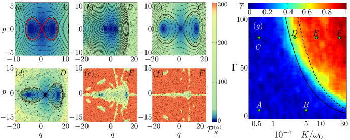
Figure 1: Regularity and chaos in phase space and in the quasienergy spectrum for $\omega_{d}/\omega_{0}=1.999866$. (a)-(f): Phase space analysis of the parameters indicated in Table 1. The black dots give the classical Poincaré sections for many different initial conditions, the red line in (a) marks the separatrix that defines the Bernoulli lemniscate, colors from blue to orange indicate the values of the participation ratio of coherent states projected in the Floquet states. (g): Measure of quantum chaos given by the average ratio $\overline{r}$ of consecutive quasienergies spacings as a function of $K/\omega_{0}$ and $\Gamma$. The six points A-F marked in (g) are the same ones chosen for the phase spaces in (a)-(f). They were selected to illustrate the behavior in the regular, mixing, and chaotic regimes. The solid black curve in (g) corresponds to Eq. (12) and indicates the parametric case, where the classical Lyapunov exponent becomes positive in the vicinity of the center of the lemniscate, while the black dashed line is given in corresponds to Eq. (13) and indicates the parameters for which chaos sets in both inside and outside the original lemniscate, which by then has disappeared.

Point	$10^{-4}K/\omega_{0}$	$\Gamma$	$n_{\text{min}}$
A	0.53	8.5	8.079
B	5.02	8.5	7.249
C	0.53	80	77.007
D	2.91	80	66.134
E	8.33	80	197.924
F	25	80	336.598

Table 1: This table gives the parameters for the points A-F marked in Fig. 1(g), whose phase diagrams are depicted in Figs. 1(a)-(f), and the corresponding values of $n_{\text{min}}$ obtained with Eq. (9).

The black dots in Fig. 1(a) designate the Poincaré sections. These points are obtained by evolving many different classical initial conditions according to Eq. (5) and collecting the values of $q$ and $p$ at each time $T_{d}$. The curves that are formed with these points coincide with the energy contours of the classical limit of the static effective Hamiltonian investigated in [23, 24, 25, 37] (see Eq. (25) in appendix C). The red curve in Fig. 1(a) is the Bernoulli lemniscate, which delineates the boundary of the double well and is characterized by the following two parameters: $\Pi=\Omega_{d}\omega_{d}/\left(\omega^{2}_{d}-\omega^{2}_{0}\right)$, where $\sqrt{2}\Pi$ is the distance from the center of the phase space to the center of the double well, and $\sqrt{2\Gamma}$, which is the half distance between the two minima of the wells, with $\Gamma=g_{3}\Pi/K$. The symmetric ellipses within the lemniscate in Fig. 1(a) are centered at the minima of the metapotential at $(\pm q_{\text{min}}\!=\!\pm\sqrt{2\Gamma},\,p_{\text{min}}=0)$, and the area within the lemniscate is equal to $4\Gamma$ (see appendix B). Using Bohr quantization rule and dimensionless coordinates $q$ and $p$, we thus have $\oint pdq=2\pi n_{\text{in}}$, and the integer number of levels inside the lemniscate is given by [24]

$$n_{\text{in}}=2\Gamma/\pi,$$ (7)

which can be measured experimentally.

We color Fig. 1(a) according to the value of the participation ratio,

$$\mathcal{P}_{\mathcal{R}}^{(\alpha)}=\frac{1}{\sum_{j}\left|\bra{\alpha}\ket{\mathcal{F}_{j}}\right|^{4}}=\frac{1}{\sum_{j}\left(\pi\mathcal{Q}_{\mathcal{F}_{j}}^{\alpha}\right)^{2}},$$ (8)

for coherent states $|\alpha\rangle$ projected in the Floquet states, where $\hat{a}|\alpha\rangle=\alpha|\alpha\rangle$, with $\alpha=(q+ip)/\sqrt{2}$, and $\mathcal{Q}_{\mathcal{F}_{j}}^{\alpha}=\left|\bra{\alpha}\ket{\mathcal{F}_{j}}\right|^{2}/\pi$ is the Husimi function of each Floquet state. The participation ratio in Eq. (8) measures the level of delocalization of a coherent state in the basis defined by $\ket{\mathcal{F}_{j}}$. The most localized coherent states are those centered at the minima of the double-well metapotential, $|\pm\alpha_{\text{min}}\rangle$, and at the center of the phase space at $(p,q)=(0,0)$ [23]. They have the smallest values of $\mathcal{P}_{R}^{(\alpha)}$, which correspond to the darkest tones of blue in Fig. 1(a).

There are two quasidegenerate Floquet states, $|\mathcal{F}_{\text{min}}\rangle$, that are highly localized at the minima of the double wells and correspond to superpositions of the two opposite-phase coherent states, $|\mathcal{F}_{\text{min}}\rangle\propto$ $|+\alpha_{\text{min}}\rangle\pm|-\alpha_{\text{min}}\rangle$ [51, 1]. These states define the Schrödinger cat states of the Kerr-cat qubit [10]. The expectation value of the number operator for these states is

$$n_{\text{min}}=\langle\mathcal{F}_{\text{min}}|\hat{n}|\mathcal{F}_{\text{min}}\rangle\approx|\alpha_{\text{min}}|^{2}=\Gamma,$$ (9)

which can be measured experimentally. This value is directly related with the number of states inside the lemniscate, $n_{\text{in}}$, given in Eq. (7).

III.1 Kerr-cat qubit disintegration

The portion of the space phase presented in Fig. 1(a) is characterized by periodic orbits, being therefore regular. However, a chaotic sea exists far away from the lemniscate, as shown in appendix B. The analysis of global chaos would classify the system with the parameters of Fig. 1(a) as being in a mixed regime, but this is not our focus. We are concerned with local chaos, which can emerge around the phase space center and destroy the Kerr-cat qubit. By increasing the strength of the nonlinearities and drive, the chaotic sea, which was once far away, expands and reaches the phase space region of interest to parametric quantum computation, that is, the region surrounding the lemniscate.

To analyze the transition to chaos in the region surrounding the center of the phase space, we vary $\Gamma$ and $K/\omega_{0}$. This is done so that the Kerr amplitude remains within values that are experimentally accessible in the present or near future, $K/\omega_{0}\in 33\times[10^{-6},10^{-4}]$ (see appendix C). The parameter $\Gamma$ is varied by changing $\Pi$, while keeping $\omega_{d}\approx 2\omega_{0}$.

To determine the onset of quantum chaos, we use the average ratio of consecutive quasienergy spacings [52, 53],

$$\tilde{r}=\frac{1}{N}\sum^{N}_{j}\text{min}\left(r_{j},\frac{1}{r_{j}}\right),\hskip 5.69046pt\text{where}\hskip 5.69046ptr_{j}=\frac{s_{j}}{s_{j-1}},$$ (10)

and $s_{j}=\epsilon_{j+1}-\epsilon_{j}$. The spectra of chaotic systems are rigid and the levels are correlated, which result in Wigner-Dyson distributions for the spacings of neighboring levels. When the symmetries of the chaotic system comply with the circular orthogonal ensemble, $\tilde{r}_{\text{COE}}\approx 0.53$. For regular systems, the levels are uncorrelated and follow Poisson statistics, so $\tilde{r}_{\text{P}}\approx 0.39$. We compute the renormalized quantity,

$$\bar{r}=\frac{\tilde{r}-\tilde{r}_{\text{P}}}{\tilde{r}_{\text{COE}}-\tilde{r}_{\text{P}}},$$ (11)

so that chaos becomes associated with $\bar{r}=1$ and regularity with $\bar{r}=0$.

In Fig. 1(g), we construct a map of regularity and chaos for the quantum system in Eq. (1). The region in red indicates that $\bar{r}\approx 1$, so the system is chaotic. This region emerges for large values of the Kerr amplitude, $K/\omega_{0}$, and $\Gamma$. The region in blue indicates regularity.

The six points A-F marked in Fig. 1(g) are chosen for a more detailed analysis in Figs. 1(a)-(f) of their corresponding phase space structures (classical analysis) and of the level of delocalization of coherent states written in the basis of Floquet states (quantum analysis). Just as in Fig. 1(a), described above, the black dots in Figs. 1(b)-(f) are associated with the Poincaré sections and the colors give the values of the participation ratio of coherent states projected in the Floquet states. It is also informative to compare Figs. 1(a)-(f) with Figs. 5(a)-(f) of appendix D, where we color the phase spaces with the Lyapunov exponent, $\lambda$, of the classical system in Eq. (5). The regular regime is defined by a zero Lyapunov exponent and chaos corresponds to positive values. There is a clear quantum-classical correspondence, where large values of $\mathcal{P}_{\mathcal{R}}^{(\alpha)}$ appear when $\lambda$ is positive.

Points A, B and C are in the regular regime. The lemniscate in Fig. 1(a) persists in Figs. 1(b)-(c), although it becomes more asymmetric. Notice that to provide more details for the lemniscate of point A, the scales in Fig. 1(a) are not the same as in Figs. 1(b)-(c).

Point B corresponds to a large value of the Kerr amplitude and we see that away from the lemniscate, the periodic orbits disappear, giving space to black dots at the edges of Fig. 1(b) and to positive Lyapunov exponents at the edges of Fig. 5(b). In spite of that, the structure of the Kerr-cat qubit survives and the value of $n_{\text{min}}$ remains close to $\Gamma$, as seen in Table 1. The resilience of the Kerr-cat qubit to a range of values of the the Kerr nonlinearity should be reassuring to the parametric quantum computation community (see also appendix C).

Point C shows what happens to point B as one approaches the classical limit, which is done by broadening the wells. By increasing $\Gamma$ while keeping $\Gamma K/\omega_{0}$ constant, we enlarge the wells without changing their shape and increase the number of levels within (cf. the values of $n_{\text{min}}$ for B and C in Table 1), thus approaching the classical picture.

Point D is in a mixed regime. The center of the double well, which is a hyperbolic point in Figs. 1(a)-(c), no longer corresponds to a single point in Fig. 1(d) and the Lyapunov exponent in this area becomes positive, as shown in Fig. 5(d). Chaos and islands of stability are seen around the structure of the asymmetric double well and chaos now exists also in the center of the structure, indicating that the lemniscate has started to disintegrate. At this stage, any activation between wells [12, 24] will happen through the chaotic region, melting away the Kerr-cat qubit.

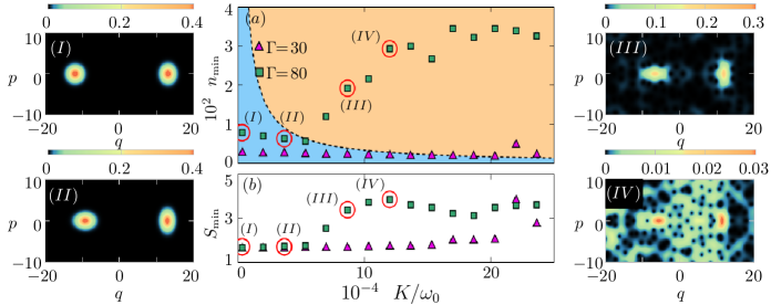
Figure 2: (a) Expectation value of the number operator, $n_{\text{min}}$, and (b) Shannon entropy, $S_{\text{min}}$, for the Floquet state $|\mathcal{F}_{\text{min}}\rangle$. The two quantities are shown as a function of the Kerr amplitude $K/\omega_{0}$ for $\Gamma=30$ (triangles) and $\Gamma=80$ (squares). In (a): The blue background indicates the regular region and the orange background indicates the chaotic region; they are separated by the same black dashed line shown in Fig. 1(g). Panels (I), (II), (III), and (IV) depict the Husimi functions for the Floquet state $|\mathcal{F}_{\text{min}}\rangle$ indicated in (a) and (b) as points (I), (II), (III), and (IV) with $K/\omega_{0}=\{0.33,3.66,8.66,12\}\times 10^{-4}$, respectively.

The values of $\Gamma$ and $K/\omega_{0}$ beyond which the intermediate regime between regularity and (local) chaos emerges follows the black solid line in Fig. 1(g). They correspond to the parameters, where the Lyapunov exponent first gets positive in the vicinity of the phase-space center (see appendix D). This solid line marks the beginning of the lemniscate disintegration and is given by

$$\Gamma K/\omega_{0}=\frac{g_{3}\Omega_{d}\omega_{d}}{\omega_{0}(\omega_{d}^{2}-\omega_{0}^{2})}\simeq 0.0187.$$ (12)

This equation shows that despite the transition to chaos, there is still ample space for the stabilization of Schrödinger cat states and for reaching large values of $K$, which are needed for fast gates.

As we move from point D [Fig. 1(d)] to points E and F [Figs. 1(e)-(f)], chaos takes over the entire phase space, the double-well structure is destroyed, and the Lyapunov exponent shown in Figs. 5(e)-(f) is positive throughout. In Fig. 1(e), we can still notice two small islands of regularity that are reminiscent of the double well and between them, the states are less delocalized than the states around the islands, while the values of $\mathcal{P}_{\mathcal{R}}^{(\alpha)}$ in Fig. 1(f) indicate near ergodicity.

In Fig. 1(g), we draw a dashed black line to indicate the parameters for which chaos close to the phase-space center and around the double well merge together leading to ergodicity. Similarly to Eq. (12), the analysis is based on the values of the Lyapunov exponents (appendix D) and the equation for the dashed line is given by

$$\Gamma K/\omega_{0}=\frac{g_{3}\Omega_{d}\omega_{d}}{\omega_{0}(\omega_{d}^{2}-\omega_{0}^{2})}\simeq 0.03347.$$ (13)

The analysis in Fig. 1 was performed using a relation between $g_{3}$ and $g_{4}$ that ensures that the parameters in Fig. 1(a) reproduce the physics in [24], where the second-order static effective Hamiltonian describes very well the experiment. There are numerous other possibilities for varying the parameters, many within experimental capabilities. Nevertheless, as we discuss in appendix C, they lead to results that are comparable to those in Fig. 1. The transition to chaos is unavoidable, although one may be able to slightly shift the values for the regularity-chaos threshold, thus changing the constants in Eqs (12)-(13).

IV Chaos detection

The experiment with the superconducting circuit performed in [24] measured the energy levels of the driven nonlinear oscillator as a function of the control parameter. However, the number of levels currently accessible to the experiment is not sufficient for the analysis of level statistics, as done in Fig. 1(g). To circumvent this issue, we propose a way to detect the transition to chaos that avoids the analysis of the quasienergy spectrum and focuses instead on the properties of the Floquet state $|\mathcal{F}_{\text{min}}\rangle$. When the system is in the regular regime, this state coincides with the Schrödinger cat state and is highly localized at the minima of the wells. As the nonlinearities increase and $|\mathcal{F}_{\text{min}}\rangle$ spreads in phase space, chaos is guaranteed to have set throughout the phase space.

In Fig. 2(a), we show $n_{\text{min}}=\langle\mathcal{F}_{\text{min}}|\hat{n}|\mathcal{F}_{\text{min}}\rangle$ as a function of $K/\omega_{0}$ for two parameters: $\Gamma=30$ (triangles) and $\Gamma=80$ (squares). The background is colored according to the results in Fig. 1(g) using that in the presence of the double well, $n_{\text{min}}\sim\Gamma$, so the region in blue is regular and orange indicates chaos. The dashed black line separating the two regions is the same as in Fig. 1(g). To complement the analysis, Fig. 2(b) makes a parallel with Fig. 2(a). It shows the behavior of the Shannon entropy for the Floquet state $|\mathcal{F}_{\text{min}}\rangle$ projected in the coherent states,

$$S_{\text{min}}=-\frac{1}{\pi}\int\mathcal{Q}^{\alpha}_{{\mathcal{F}_{\text{min}}}}\ln\left(\mathcal{Q}^{\alpha}_{{\mathcal{F}_{\text{min}}}}\right)\,d^{2}\alpha,$$ (14)

as function of $K/\omega_{0}$ for $\Gamma=30$ (triangles) and $\Gamma=80$ (squares).

We start by describing the results for $\Gamma=80$ (squares) in Fig. 2(a). In the regular regime, $n_{\text{min}}$ decays linearly with the Kerr amplitude. To better explain this behavior, we select two points in Fig. 2(a), indicated as (I) and (II), and analyze their respective Husimi functions on the left panels (I) and (II). As expected, the Husimi functions for these two $|\mathcal{F}_{\text{min}}\rangle$ are localized at the minima of the double well, at $q=\pm\sqrt{2\Gamma}\approx\pm 13$. Comparing panel (I) and panel (II), we see that as $K/\omega_{0}$ increases, the structure of the Husimi function becomes more asymmetric and the area of the lemniscate decreases, which reduces the value of $n_{\text{min}}$ [see also Figs. 1(a)-(c)]. At the same time, since the Husimi functions remain localized in panels (I) and (II), the values of the Shannon entropy for these two cases in Fig. 2(b) remain comparable.

For $\Gamma=80$ (squares), as we enter the chaotic region, $n_{\text{min}}$ in Fig. 2(a) and $S_{\text{min}}$ in Fig. 2(b) grow with $K/\omega_{0}$. This can be understood by analyzing the Husimi functions for the points (III) and (IV) shown on the panels to the right of Figs. 2(a)-(b). The parameters for point (III) are equivalent to those in Fig. 1(e), where there are two islands of instability close to the original minima of the double well. This explains why $|\mathcal{F}_{\text{min}}\rangle$ in panel (III) shows some level of confinement around the islands, although the state is visibly more delocalized than those in panels (I) and (II). The parameters for point (IV) are equivalent to those in Fig. 1(f), where the system approaches ergodicity, so the Husimi function in panel (IV) is spread out. As the level of delocalization of $|\mathcal{F}_{\text{min}}\rangle$ increase from point (II) to (III) and from point (III) to (IV), $n_{\text{min}}$ and $S_{\text{min}}$ naturally grow in Figs.2(a)-(b).

For values of $K/\omega_{0}$ at and beyond point (IV), the double well is completely destroyed, so it no longer makes sense to talk about the number of states inside the lemniscate. In this case, all Floquet states are delocalized, including $|\mathcal{F}_{\text{min}}\rangle$, which is now hard to distinguish from the others, so $n_{\text{min}}$ and $S_{\text{min}}$ fluctuate with $K/\omega_{0}$.

The behavior of $n_{\text{min}}$ and $S_{\text{min}}$ as a function of the Kerr amplitude for $\Gamma=30$ [triangles in Figs. 2(a)-(b)] is equivalent to that for $\Gamma=80$. The difference is that for $\Gamma=30$, the onset of chaos and the consequent growth of $n_{\text{min}}$ and $S_{\text{min}}$ with $K/\omega_{0}$ require larger values of the Kerr amplitude than for $\Gamma=80$, as indeed seen in Figs. 2(a)-(b).

In summary, the disintegration of the double well and its substitution by chaos can be detected from the analysis of the spread of the Schrödinger cat states in phase space and its eventual disintegration. This can be done by directly investigating the Husimi or Wigner functions of these states in phase space for different values of the system parameters or by quantifying their spread with the occupation number $n_{\text{min}}$ or an entropy, such as $S_{\text{min}}$. The growth of $n_{\text{min}}$ and $S_{\text{min}}$ signals the departure from the regular to the chaotic regime.

V Discussion

Our work brings to light the danger of the onset of chaos for Kerr parametric oscillators, which puts a limit on the ranges of parameters that can be employed for qubit implementation. Combining quantum and classical analysis, we determined the threshold for the rupture of the Kerr-cat qubit, which happens when chaos first sets in around the center of the qubit double-well structure. Important extensions to this work include the role of dissipation and the analysis of the limitations that chaos may impose to parametric gates in transmon and fluxonium arrays.

By increasing the nonlinearities and driving amplitude, we showed that the Schrödinger cat states of the Kerr-cat qubit, which are initially at the bottom of the wells, spread and eventually disintegrate. Once these states are lost, chaos is certain to have spread throughout the phase space. The process of disintegration could be experimentally observed with available technology by measuring the Wigner functions of the cat states.

The results in this work indicate that on the same platform of superconducting circuits, one can either engineer bosonic qubits for quantum technologies or develop chaos to address fundamental questions. This opens up a new avenue of research for superconducting circuits. They could be used, for example, to investigate how chaos affects the spread of quantum information in phase space and whether chaos can enhance the tunneling rate between islands of stability.

Appendix A Quantum and Classical Hamiltonian

The driven SNAIL transmon is analogous to an asymmetric driven pendulum. By Taylor expanding the potential, the Hamiltonian is given by [24]

$$\frac{\hat{H}(t)}{\hbar}=\omega_{0}\hat{a}^{\dagger}\hat{a} +\sum_{m=3}^{\infty}\frac{g_{m}}{m}\left(\hat{a}^{\dagger}+\hat{a}\right)^{m}$$ (15)

$$-i\Omega_{d}\left(\hat{a}-\hat{a}^{\dagger}\right)\cos(\omega_{d}t),$$

where $\omega_{0}$ is the bare frequency of the oscillator, $g_{m}$’s are the circuit nonlinearities, $g_{m}\ll\omega_{0}$, and the drive is characterized by its amplitude $\Omega_{d}$ and frequency $\omega_{d}$. The nonlinearity originates from an arrangement of Josephson junctions in the SNAIL transmon and can be tuned with a magnetic flux. Only the third and fourth-rank nonlinearities were relevant in the experiments in [24, 25]), which gives our Eq. (1) in the main text for the quantum Hamiltonian,

$$\frac{\hat{H}(t)}{\hbar}=\omega_{0}\hat{a}^{\dagger}\hat{a} +\frac{g_{3}}{3}(\hat{a}+\hat{a}^{\dagger})^{3}+\frac{g_{4}}{4}(\hat{a}+\hat{a}^{\dagger})^{4}$$ (16)

$$-i\Omega_{d}(\hat{a}-\hat{a}^{\dagger})\cos(\omega_{d}t).$$

To derive the classical Hamiltonian, we write

$$\hat{a}=\sqrt{\frac{N_{\text{eff}}}{2}}\left(\hat{q}+i\hat{p}\right),$$ (17)

and

$$[\hat{q},\hat{p}]=\frac{i}{N_{\text{eff}}},$$

so that the classical limit can be reached by taking $N_{\text{eff}}\rightarrow\infty$, since $\hat{q}\rightarrow q$ and $\hat{p}\rightarrow p$. This way, the quantum Hamiltonian,

$$\frac{\hat{H}(t)}{\hbar} = \frac{\omega_{0}N_{\text{eff}}}{2}\left(\hat{q}-i\hat{p}\right)\left(\hat{q}+i\hat{p}\right)+\sum^{4}_{m=3}\frac{g_{m}}{m}(\sqrt{2N_{\text{eff}}}\hat{q})^{m}$$ (18)

$$+ \Omega_{d}\sqrt{2\,N_{\text{eff}}}\,\hat{p}\,\cos\omega_{d}t,$$

leads to the classical Hamiltonian (with $\hbar=1$),

$$h_{cl}(t) = \frac{\omega_{0}^{cl}}{2}\left(q^{2}+p^{2}\right)+\frac{2\sqrt{2}}{3}g_{3}^{cl}q^{3}+g_{4}^{cl}q^{4}$$ (19)

$$+ \sqrt{2}\Omega_{d}^{cl}p\cos\left(\omega_{d}t\right),$$

where

$$\omega_{0}=\omega_{0}^{cl}/N_{\text{eff}},\hskip 8.5359ptg_{3}=g_{3}^{cl}/\sqrt{N^{3}_{\text{eff}}},$$

$$g_{4}=g_{4}^{cl}/N_{\text{eff}}^{2},\hskip 8.5359pt\text{and}\hskip 8.5359pt\Omega_{d}=\Omega_{d}^{cl}/\sqrt{N_{\text{eff}}}.$$

In the main text, we fix

$$N_{\text{eff}}=1.$$

Appendix B Emergence of the Bernoulli lemniscate

To better understand the origin of the lemniscate in Fig. 1(a) and where it emerges in the phase space, let us start by analyzing the classical static Hamiltonian in Eq. (6),

$$h_{0}=\frac{\omega_{0}}{2}\left(q^{2}+p^{2}\right)+\frac{\sqrt{2^{3}}}{3}g_{3}q^{3}+g_{4}q^{4}.$$ (20)

It describes a quartic asymmetric oscillator, that presents three stationary (critical) points with $p=0$. They are the minima

$$(q_{0},p_{0}) = (0,0),$$

$$(q_{1},p_{1}) = (d_{-},0),$$

and the hyperbolic point

$$(q_{2},p_{2})=(d_{+},0),$$

where $d_{\pm}=\sqrt{2}\left(-g_{3}\pm\sqrt{g^{2}_{3}-2g_{4}\omega_{0}}\right)/(4g_{4})$. The condition $g_{3}^{2}-2g_{4}\omega_{0}>0$ ensures that $d_{\pm}$ is real.

The linearized Hamilton equations around a critical point $\{q_{c},p_{c}\}$ of $h_{0}$ satisfies the following linear differential equations,

$$\begin{pmatrix}\dot{q}\\ \dot{p}\end{pmatrix}=\begin{pmatrix}0&\omega_{0}\\ -\omega_{0}\!-\!4\sqrt{2}g_{3}q_{c}\!-\!12g_{4}q_{c}^{2}&0\\ \end{pmatrix}\begin{pmatrix}q\!-\!q_{c}\\ p\!-\!q_{c}\end{pmatrix}.$$ (21)

The stability or instability around $\{q_{c},p_{c}\}$ is determined by the eigenvalues $\lambda_{m}$ of the matrix constructed in Eq. 21. If the eigenvalues are complex numbers, $\lambda_{m}=i\,\tilde{\omega}_{m}$, the orbits in the neighborhood of the critical point are periodic and have frequencies $\tilde{\omega}_{m}$. If the eigenvalues of the matrix are real, then the critical point is unstable and its Lyapunov exponent is equal to $\text{max}(\lambda_{m})$.

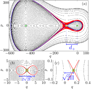
Figure 3: Asymmetric and symmetric double wells. (a) Phase space metapotential of the classical Hamiltonian $h_{cl}(t)$ in Eq. (5) representing a large asymmetric double well. Black points are used for regular orbits. The red points indicate orbits with positive Lyapunov exponents (chaos). The three green symbols indicate the critical points: square for $(q_{1},p_{1})=(d_{-},0)$, cross for $(q_{2},p_{2})=(d_{+},0)$, and circle for $(q_{0},p_{0})=(0,0)$. The blue line is the separatrix of the asymmetric double well. (b) Enlarged image of panel (a) close to the point $(0,0)$, providing a view of the additional symmetric double well that emerges at the phase space center. The red line is the Bernoulli lemniscate. The distance between the two minima is $2\sqrt{2\Gamma}$. (c) Enlarged image of panel (b) close to the point $(0,0)$. The distance between the phase space center $(0,0)$ and the hyperbolic point of the Bernoulli lemniscate is $\sqrt{2}\Pi$.

In Fig. 3(a), we show the Poincaré sections (black lines) for the driven system described by $h_{cl}(t)$ in Eq. (5) with a frequency $\omega_{d}$ that is nearly twice $\omega_{0}$ and with the parameters used in the experiment in [24] and in Fig. 1(a). The stationary points of $h_{0}$ are marked with green symbols: square for $(q_{1},p_{1})$, cross for $(q_{2},p_{2})$, and circle for $(q_{0},p_{0})$. The blue line crossing at the hyperbolic point $(q_{2},p_{2})$ is the separatrix of the big asymmetric double well. The red points indicate a chaotic sea that appears in the vicinity of the separatrix. Around the minima, there are periodic orbits with frequencies $\tilde{\omega}$ that are related to the minimum that they surround. Close to $(q_{0},p_{0})$, the orbits have frequencies $\tilde{\omega}_{0}=\omega_{0}$ and close to $(q_{1},p_{1})$, the orbits have frequencies $\tilde{\omega}_{1}=\sqrt{\omega_{0}b(g_{3}+b)}/\sqrt{g_{4}}$, while at the hyperbolic point $(q_{2},p_{2})$, the Lyapunov exponent is positive and given by $\lambda=\sqrt{\omega_{0}b(g_{3}-b)}/\sqrt{g_{4}}$, where $b=\sqrt{g^{2}_{3}-2g_{4}\omega_{0}}$.

B.1 Double well at the phase space center

Close to the stationary point $(q_{0},p_{0})=(0,0)$ at the center of the phase space, there is a bifurcation caused by the chosen driving frequency, $\omega_{d}\simeq 2\omega_{0}$, that gives rise to another double-well structure. This is better seen in Fig. 3(b), where we enlarge the area around $(q_{0},p_{0})$. The entire analysis developed in the main text concerns this region of the phase space.

The double-well structure in Fig. 3(b) also exhibits three critical points: two minima and a hyperbolic point. Notice that the hyperbolic point of this double well is very close to phase space center $(0,0)$. The separatrix is indicated with the red line, which corresponds to the Bernoulli lemniscate given by

$$(q^{2}+p^{2})^{2}=4\Gamma(q^{2}-p^{2}),$$

and in polar coordinates by

$$r^{2}(\theta)=4\Gamma\cos(2\theta),$$

where the focal distance is $\sqrt{2\Gamma}$. The surface area corresponds to

$$4\int^{\pi/4}_{0}\int^{r(\theta)}_{0}\!\!r\,dr\,d\theta=4\Gamma,$$ (22)

which is a result used to obtain Eq. (7) in the main text.

In Fig. 3(c), $\sqrt{2}\Pi$ is the distance between the phase space center $(0,0)$ and the center (hyperbolic point) of the Bernoulli lemniscate. The separation between the two points can be understood as follows. The dynamics around the critical point $(0,0)$ is given by

$$q(t)=q_{0}(t)+q_{r}(t),$$

where $q_{0}(t)$ is the homogeneous solution obtained with the undriven classical Hamiltonian $h_{0}$ and $q_{r}(t)$ is obtained from the linear terms of the Hamilton equations for the driven case, so that

$$\ddot{q}_{r}+\omega^{2}_{0}q_{r}=-\sqrt{2}\omega_{d}\Omega_{d}\sin\omega_{d}t,$$

and

$$q_{r}(t)=\sqrt{2}\Pi\sin(\omega_{d}t),$$

where

$$\Pi=\Omega_{d}\omega_{d}/\left(\omega^{2}_{d}-\omega^{2}_{0}\right).$$

The linear response associated with $q_{r}(t)$ causes a translation of the center of the lemniscate by the amplitude $\sqrt{2}\Pi$. Therefore, as one can see from Figs. 3(a)-(c), the condition for the existence of a well-defined inner double-well structure centered close to $(0,0)$ is

$$|\sqrt{2}\Pi|+|\sqrt{2\Gamma}|<|d_{+}|.$$ (23)

In Table 2, we complement Table 1 of the main text by providing the values of $\sqrt{2\Gamma}/|d_{+}|$ and $\sqrt{2}\Pi/|d_{+}|$. All points, except for point F, satisfy the inequality in Eq. (23). For point F, the lemniscate is already destroyed by chaos.

Point	$10^{-4}K/\omega_{0}$	$\Gamma$	$n_{\text{min}}$	$\sqrt{2\Gamma}/|d_{+}|$	$\sqrt{2}\Pi/|d_{+}|$
A	0.53	8.5	8.079	0.04122	0.00148492
B	5.02	8.5	7.249	0.141397	0.0157244
C	0.53	80	77.007	0.12647	0.0140573
D	2.91	80	66.134	0.29577	0.0769191
E	8.33	80	197.924	0.49995	0.219769
F	25	80	336.598	0.86594	0.659321

Table 2: This table is the same as Table 1 of the main text, where the parameters for the points A-F marked in Fig. 1(g) are provided, but now the values of $\sqrt{2\Gamma}/|d_{+}|$ and $\sqrt{2}\Pi/|d_{+}|$ are also given.

Appendix C Control parameters

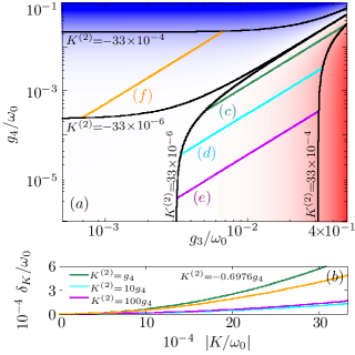
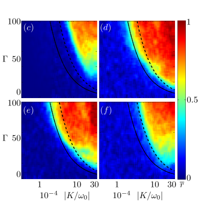
Figure 4: (a) Kerr amplitude $K^{(2)}$ of the second-order effective Hamiltonian (in color) as a function of $g_{3}/\omega_{0}$ and $g_{4}/\omega_{0}$. Red is used for $K^{(2)}>0$ and blue for $K^{(2)}<0$; the solid black lines mark constant values of $K^{(2)}$; the green line marked as (c) is for $K^{(2)}=g_{4}$, the cyan line (d) is for $K^{(2)}=10g_{4}$, the purple line (e) is for $K^{(2)}=100g_{4}$, and the orange line (f) is for $K^{(2)}=-0.6976g_{4}$. (b) Absolute difference between $K^{(2)}$ and $K$ as a function of $|K/\omega_{0}|$ for different choices of $K^{(2)}=\mathcal{C}g_{4}$, as indicated. (c)-(f): Measure of quantum chaos given by the average ratio $\overline{r}$ of consecutive quasienergies spacings as a function of $K/\omega_{0}$ and $\Gamma$, for $\omega_{d}/\omega_{0}=1.999866$ and (c) $K^{(2)}/g_{4}=1$, (d) $K^{(2)}/g_{4}=10$, (e) $K^{(2)}/g_{4}=100$, and $K^{(2)}/g_{4}=-0.6976$. The solid black curve indicates the parametric case, where the classical Lyapunov exponent becomes positive in the vicinity of the center of the lemniscate, and the dashed black curve indicates the parameters for which chaos sets in both inside and outside the original lemniscate.

In the main text, the values of $K/\omega_{0}$ are varied parametrically by varying $g_{3}/\omega_{0}$ and $g_{4}/\omega_{0}$ according to the equation

$$g_{4}=\frac{20g_{3}^{2}}{69\omega_{0}}.$$ (24)

This choice is made to guarantee that we reproduce the scenario in [24], where the second-order effective Hamiltonian describes very well the experiment. The second-order effective Hamiltonian is given by [24],

$$\frac{\hat{H}^{(2)}_{\mathrm{eff}}}{\hbar}=-K^{(2)}\hat{a}^{\dagger 2}\hat{a}^{2}+\epsilon_{2}^{(2)}(\hat{a}^{\dagger 2}+\hat{a}^{2}),$$ (25)

where

$$K^{(2)}=-\frac{3g_{4}}{2}+\frac{10g_{3}^{2}}{3\omega_{0}},$$ (26)

and $\epsilon_{2}^{(2)}=2g_{3}\Omega_{d}/(3\omega_{0})$. Equation (24) is the same as Eq. (26) when $K^{(2)}=10g_{4}$. In this section, we show what happens to the analysis in Fig. 1(g) for other choices of ${\cal C}$ in $K^{(2)}={\cal C}\,g_{4}$.

In Fig. 4(a), we show in color the values of $K^{(2)}$ as a function of $g_{3}/\omega_{0}$ and $g_{4}/\omega_{0}$. Blue gradient is used when $K^{(2)}<0$ and red gradient for $K^{(2)}>0$. The green, cyan, purple, and orange lines indicate the examples where ${\cal C}=\{1,10,100,-0.6976\}$, respectively. In Fig. 4(b), we use the difference $\delta_{K}=|K-K^{(2)}|$ to compare $K^{(2)}$ and $K$. The behavior of $\delta_{K}$ with ${\cal C}$ is non-monotonic. The best match between $K$ and $K^{(2)}$ happens for $K^{(2)}=10g_{4}$ (cyan line), which justifies the use of this choice for the analysis in the main text.

We notice that for the experimental parameter $K/\omega_{0}=0.32/6000$ used in [24], our choice of $K^{(2)}=10g_{4}$ implies that $g_{3}/\omega_{0}=25.7371/6000$, which is very close to the experimental value $g_{3}/\omega_{0}=30/6000$ used in that same work. The example ${\cal C}=-0.6976$ is selected by also using the parameters $g_{3}/\omega_{0}=25.7371/6000$ and $K^{(2)}/\omega_{0}=-0.32/6000$, with the difference that $K^{(2)}$ is now negative. We investigate ${\cal C}=-0.6976$, because negative Kerr amplitudes are also experimentally available.

Figure 4(d) is exactly the same as Fig. 1(g) of the main text. It shows the average value of the quantum chaos indicator $\bar{r}$ as a function of $\Gamma$ and $K/\omega_{0}$. To complement the analysis of the regular to chaos transition performed in the main text, we show in Fig. 4(c), Fig. 4(e), and Fig. 4(f) the results for $\bar{r}$ as a function of $\Gamma$ and $K/\omega_{0}$ for $K^{(2)}=g_{4}$, $K^{(2)}=100g_{4}$, and $K^{(2)}=-0.6976g_{4}$, respectively. The results are comparable, although for $K^{(2)}=g_{4}$ in Fig. 4(c), we see that the transition to chaos gets shifted to larger values of $\Gamma$ and $K/\omega_{0}$.

There are numerous ways in which the parameters of the Hamiltonian may be varied. There are various paths that can be taken to change $g_{3}$ and $g_{4}$ that are not necessarily linear, as those in Fig. 4, but the relationship in Eq. (12) is general. An important conclusion derived from of our studies is that the onset of chaos is unavoidable for large nonlinearities and drive, but in spite of that, there is still ample space to remain in the regular regime, where Schrödinger cat states are stable and gates can be realized.

Appendix D Lyapunov exponent

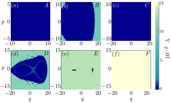
Figure 5: (a)-(f): Lyapunov exponents for the same phase spaces shown in Fig. 1(a)-(f), corresponding to the points in Table 1. Zero Lyapunov exponent (dark blue) indicates regularity.

The Lyapunov exponents are asymptotic measures that characterize the average rate of growth (or shrinking) of small perturbations along the solutions of a dynamical system. In regular systems, the distance $\textbf{x}(t)$ between a given trajectory and another trajectory infinitesimally close to it, obtained with a small perturbation in the initial conditions, remains close to zero or increases at most algebraically as time evolves. In chaotic systems, this distance diverges exponentially in time,

$$|\delta\textbf{x}(t)|\sim e^{\lambda t}|\delta\textbf{x}(0)|.$$ (27)

The divergence in the equation above is characterized by the Lyapunov exponent [54],

$$\lambda=\lim_{t\rightarrow\infty}\lim_{|\delta\textbf{x}|\rightarrow 0}\frac{1}{t}\ln\frac{|\delta\textbf{x}(t)|}{|\delta\textbf{x}_{0}|},$$ (28)

where $|\cdot|$ is a norm in the phase space. In the case of regular (stable) trajectories, $\lambda=0$, while chaos implies $\lambda>0$.

In Figs. 5(a)-(f), we color the same phase spaces studied in Figs. 1(a)-(f) with the values of the Lyapunov exponent $\lambda$. The exponents are obtained for the classical system in Eq. (5) using various initial conditions. Points A and C in Fig. 1(a) and Fig. 1(c) have only regular trajectories, while chaotic orbits appear at the edges of Fig. 1(b). Point D represents a mixed region, where in addition to chaos at the edges of the figure, we also find positive Lyapunov exponents in the vicinity of the hyperbolic point of the double well metapotential. As discussed in the main text, point D illustrates the beginning of the disintegration of the double well. In Fig. 1(e), there are two islands of instability associated with the minima of what used to be the double-well structure, while in Fig. 1(f) chaos becomes ubiquitous.

References

- Mirrahimi et al. [2014] M. Mirrahimi, Z. Leghtas, V. V. Albert, S. Touzard, R. J. Schoelkopf, L. Jiang, and M. H. Devoret, Dynamically protected cat-qubits: a new paradigm for universal quantum computation, New J. Phys. 16, 045014 (2014).
- Haroche [2013] S. Haroche, Nobel lecture: Controlling photons in a box and exploring the quantum to classical boundary, Rev. Mod. Phys. 85, 1083 (2013).
- Wineland [2013] D. J. Wineland, Nobel lecture: Superposition, entanglement, and raising schrödinger’s cat, Rev. Mod. Phys. 85, 1103 (2013).
- Leghtas et al. [2015] Z. Leghtas, S. Touzard, I. M. Pop, A. Kou, B. Vlastakis, A. Petrenko, K. M. Sliwa, A. Narla, S. Shankar, M. J. Hatridge, M. Reagor, L. Frunzio, R. J. Schoelkopf, M. Mirrahimi, and M. H. Devoret, Confining the state of light to a quantum manifold by engineered two-photon loss, Science 347, 853 (2015).
- Puri et al. [2017] S. Puri, S. Boutin, and A. Blais, Engineering the quantum states of light in a Kerr-nonlinear resonator by two-photon driving, npj Quantum Inf. 3, 18 (2017).
- Goto et al. [2018] H. Goto, Z. Lin, and Y. Nakamura, Boltzmann sampling from the Ising model using quantum heating of coupled nonlinear oscillators, Sci. Rep. 8, 7154 (2018).
- Goto [2019] H. Goto, Quantum computation based on quantum adiabatic bifurcations of Kerr-nonlinear parametric oscillators, J. Phys. Soc. Japan 88, 061015 (2019).
- Kwon et al. [2022] S. Kwon, S. Watabe, and J.-S. Tsai, Autonomous quantum error correction in a four-photon Kerr parametric oscillator, npj Quantum Inf. 8, 40 (2022).
- He et al. [2023] X. L. He, Y. Lu, D. Q. Bao, H. Xue, W. B. Jiang, Z. Wang, A. F. Roudsari, P. Delsing, J. S. Tsai, and Z. R. Lin, Fast generation of schrödinger cat states using a Kerr-tunable superconducting resonator, Nat. Comm. 14, 6358 (2023).
- Grimm et al. [2020] A. Grimm, N. E. Frattini, S. Puri, S. O. Mundhada, S. Touzard, M. Mirrahimi, S. M. Girvin, S. Shankar, and M. H. Devoret, Stabilization and operation of a Kerr-cat qubit, Nature 584, 205 (2020).
- Frattini et al. [2017] N. E. Frattini, U. Vool, S. Shankar, A. Narla, K. M. Sliwa, and M. H. Devoret, 3-wave mixing Josephson dipole element, Appl. Phys. Lett. 110, 222603 (2017).
- Marthaler and Dykman [2006] M. Marthaler and M. I. Dykman, Switching via quantum activation: A parametrically modulated oscillator, Phys. Rev. A 73, 042108 (2006).
- Lin et al. [2015] Z. R. Lin, Y. Nakamura, and M. I. Dykman, Critical fluctuations and the rates of interstate switching near the excitation threshold of a quantum parametric oscillator, Phys. Rev. E 92, 022105 (2015).
- Marthaler and Dykman [2007] M. Marthaler and M. I. Dykman, Quantum interference in the classically forbidden region: A parametric oscillator, Phys. Rev. A 76, 010102 (2007).
- Peano et al. [2012] V. Peano, M. Marthaler, and M. I. Dykman, Sharp tunneling peaks in a parametric oscillator: Quantum resonances missing in the rotating wave approximation, Phys. Rev. Lett. 109, 090401 (2012).
- Reynoso et al. [2023] M. A. P. Reynoso, D. J. Nader, J. Chávez-Carlos, B. E. Ordaz-Mendoza, R. G. Cortiñas, V. S. Batista, S. Lerma-Hernández, F. Pérez-Bernal, and L. F. Santos, Quantum tunneling and level crossings in the squeeze-driven Kerr oscillator, Phys. Rev. A 108, 033709 (2023).
- Iyama et al. [2023] D. Iyama, T. Kamiya, S. Fujii, H. Mukai, Y. Zhou, T. Nagase, A. Tomonaga, R. Wang, J.-J. Xue, S. Watabe, S. Kwon, and J.-S. Tsai, Observation and manipulation of quantum interference in a superconducting Kerr parametric oscillator (2023), arXiv:2306.12299 .
- Roberts and Clerk [2020] D. Roberts and A. A. Clerk, Driven-dissipative quantum Kerr resonators: New exact solutions, photon blockade and quantum bistability, Phys. Rev. X 10, 021022 (2020).
- Dykman [2012] M. Dykman, Fluctuating Nonlinear Oscillators From Nanomechanics to Quantum Superconducting Circuits (Oxford University Press, 2012).
- Venkatraman et al. [2022a] J. Venkatraman, X. Xiao, R. G. Cortiñas, A. Eickbusch, and M. H. Devoret, Static effective Hamiltonian of a rapidly driven nonlinear system, Phys. Rev. Lett. 129, 100601 (2022a).
- Xiao et al. [2023a] X. Xiao, J. Venkatraman, R. G. Cortiñas, S. Chowdhury, and M. H. Devoret, A diagrammatic method to compute the effective Hamiltonian of driven nonlinear oscillators (2023a), arXiv:2304.13656 .
- Zhang et al. [2016] L. Zhang, B. Zhao, T. Devakul, and D. A. Huse, Many-body localization phase transition: A simplified strong-randomness approximate renormalization group, Phys. Rev. B 93, 224201 (2016).
- Chávez-Carlos et al. [2023] J. Chávez-Carlos, T. L. M. Lezama, R. G. Cortiñas, J. Venkatraman, M. H. Devoret, V. S. Batista, F. Pérez-Bernal, and L. F. Santos, Spectral kissing and its dynamical consequences in the squeeze-driven Kerr oscillator, npj Quantum Inf. 9, 76 (2023).
- Frattini et al. [2022] N. E. Frattini, R. G. Cortiñas, J. Venkatraman, X. Xiao, Q. Su, C. U. Lei, B. J. Chapman, V. R. Joshi, S. M. Girvin, R. J. Schoelkopf, S. Puri, and M. H. Devoret, The squeezed Kerr oscillator: Spectral kissing and phase-flip robustness (2022), arXiv:2209.03934 .
- Venkatraman et al. [2022b] J. Venkatraman, R. G. Cortinas, N. E. Frattini, X. Xiao, and M. H. Devoret, Quantum interference of tunneling paths under a double-well barrier (2022b), arXiv:2211.04605 .
- Campagne-Ibarcq et al. [2020] P. Campagne-Ibarcq, A. Eickbusch, S. Touzard, E. Zalys-Geller, N. E. Frattini, V. V. Sivak, P. Reinhold, S. Puri, S. Shankar, R. J. Schoelkopf, L. Frunzio, M. Mirrahimi, and M. H. Devoret, Quantum error correction of a qubit encoded in grid states of an oscillator, Nature 584, 368 (2020).
- Georgeot and Shepelyansky [2000a] B. Georgeot and D. L. Shepelyansky, Emergence of quantum chaos in the quantum computer core and how to manage it, Phys. Rev. E 62, 6366 (2000a).
- Georgeot and Shepelyansky [2000b] B. Georgeot and D. L. Shepelyansky, Quantum chaos border for quantum computing, Phys. Rev. E 62, 3504 (2000b).
- Braun [2002] D. Braun, Quantum chaos and quantum algorithms, Phys. Rev. A 65, 042317 (2002).
- Silvestrov et al. [2001] P. G. Silvestrov, H. Schomerus, and C. W. J. Beenakker, Limits to Error Correction in Quantum Chaos, Phys. Rev. Lett. 86, 5192 (2001).
- Shenker and Stanford [2015] S. H. Shenker and D. Stanford, Stringy effects in scrambling, JHEP 2015 (5), 132.
- Maldacena et al. [2016] J. Maldacena, S. H. Shenker, and D. Stanford, A bound on chaos, J. High Energy Phys. 2016 (8), 106.
- Gärttner et al. [2017] M. Gärttner, J. G. Bohnet, A. Safavi-Naini, M. L. Wall, J. J. Bollinger, and A. M. Rey, Measuring out-of-time-order correlations and multiple quantum spectra in a trapped-ion quantum magnet, Nat. Phys. 13, 781 (2017).
- Niknam et al. [2020] M. Niknam, L. F. Santos, and D. G. Cory, Sensitivity of quantum information to environment perturbations measured with a nonlocal out-of-time-order correlation function, Phys. Rev. Research 2, 013200 (2020).
- Goto and Kanao [2021] H. Goto and T. Kanao, Chaos in coupled Kerr-nonlinear parametric oscillators, Phys. Rev. Res. 3, 043196 (2021).
- Cohen et al. [2023] J. Cohen, A. Petrescu, R. Shillito, and A. Blais, Reminiscence of classical chaos in driven transmons, PRX Quantum 4, 020312 (2023).
- García-Mata et al. [2023] I. García-Mata, R. G. Cortiñas, X. Xiao, J. Chávez-Carlos, V. S. Batista, L. F. Santos, and D. A. Wisniacki, Effective versus Floquet theory for the Kerr parametric oscillator (2023), arXiv:2309.12516 [quant-ph] .
- Xiao et al. [2023b] X. Xiao, J. Venkatraman, R. G. Cortiñas, S. Chowdhury, and M. H. Devoret, A diagrammatic method to compute the effective Hamiltonian of driven nonlinear oscillators (2023b), arXiv:2304.13656 [quant-ph] .
- Blais et al. [2021] A. Blais, A. L. Grimsmo, S. M. Girvin, and A. Wallraff, Circuit quantum electrodynamics, Rev. Mod. Phys. 93, 025005 (2021).
- Hillmann et al. [2020] T. Hillmann, F. Quijandría, G. Johansson, A. Ferraro, S. Gasparinetti, and G. Ferrini, Universal gate set for continuous-variable quantum computation with microwave circuits, Phys. Rev. Lett. 125, 160501 (2020).
- Noguchi et al. [2020] A. Noguchi, A. Osada, S. Masuda, S. Kono, K. Heya, S. P. Wolski, H. Takahashi, T. Sugiyama, D. Lachance-Quirion, and Y. Nakamura, Fast parametric two-qubit gates with suppressed residual interaction using the second-order nonlinearity of a cubic transmon, Phys. Rev. A 102, 062408 (2020).
- Moore et al. [1995] F. L. Moore, J. C. Robinson, C. F. Bharucha, B. Sundaram, and M. G. Raizen, Atom optics realization of the quantum -kicked rotor, Phys. Rev. Lett. 75, 4598 (1995).
- Weinstein et al. [2002] Y. S. Weinstein, S. Lloyd, J. Emerson, and D. G. Cory, Experimental implementation of the quantum baker’s map, Phys. Rev. Lett. 89, 157902 (2002).
- Chaudhury et al. [2009] S. Chaudhury, A. Smith, B. E. Anderson, S. Ghose, and P. S. Jessen, Quantum signatures of chaos in a kicked top, Nature 461, 768–771 (2009).
- Lemos et al. [2012] G. B. Lemos, R. M. Gomes, S. P. Walborn, P. H. Souto Ribeiro, and F. Toscano, Experimental observation of quantum chaos in a beam of light, Nat. Comm. 3, 1211 (2012).
- Hensinger et al. [2001] W. K. Hensinger, H. Häffner, A. Browaeys, N. R. Heckenberg, K. Helmerson, C. McKenzie, G. J. Milburn, W. D. Phillips, S. L. Rolston, H. Rubinsztein-Dunlop, and B. Upcroft, Dynamical tunnelling of ultracold atoms, Nature 412, 52 (2001).
- Steck et al. [2001] D. A. Steck, W. H. Oskay, and M. G. Raizen, Observation of Chaos-Assisted Tunneling Between Islands of Stability, Science 293, 274 (2001).
- Frattini et al. [2018] N. E. Frattini, V. V. Sivak, A. Lingenfelter, S. Shankar, and M. H. Devoret, Optimizing the nonlinearity and dissipation of a SNAIL parametric amplifier for dynamic range, Phys. Rev. Appl. 10, 054020 (2018).
- Sivak et al. [2019] V. Sivak, N. Frattini, V. Joshi, A. Lingenfelter, S. Shankar, and M. Devoret, Kerr-free three-wave mixing in superconducting quantum circuits, Phys. Rev. Appl. 11, 054060 (2019).
- Holthaus [2015] M. Holthaus, Floquet engineering with quasienergy bands of periodically driven optical lattices, J.Phys. B 49, 013001 (2015).
- Cochrane et al. [1999] P. T. Cochrane, G. J. Milburn, and W. J. Munro, Macroscopically distinct quantum-superposition states as a bosonic code for amplitude damping, Phys. Rev. A 59, 2631 (1999).
- Oganesyan and Huse [2007] V. Oganesyan and D. A. Huse, Localization of interacting fermions at high temperature, Phys. Rev. B 75, 155111 (2007).
- Atas et al. [2013] Y. Y. Atas, E. Bogomolny, O. Giraud, and G. Roux, Distribution of the ratio of consecutive level spacings in random matrix ensembles, Phys. Rev. Lett. 110, 084101 (2013).
- Skokos [2008] C. Skokos, The Lyapunov characteristic exponents and their computation, Lect. Notes Phys. 790, 63 (2008).