An infrared FWHM-$K_{2}$ correlation to uncover highly reddened quiescent black holes

Among the sample of Galactic transient X-ray binaries (SXTs) discovered to date, about 70 have been proposed as likely candidates to host a black hole. Yet, only 19 have been dynamically confirmed. Such a reliable confirmation requires phase-resolved spectroscopy of their companion stars, which is generally feasible when the system is in a quiescent state. However, since most of the SXT population lies in the galactic plane, which is strongly affected by interstellar extinction, their optical brightness during quiescence usually falls beyond the capabilities of the current instrumentation ($R\gtrsim 22$). To overcome these limitations and thereby increase the number of confirmed Galactic black holes, a correlation between the full-width at half maximum (FWHM) of the H$\alpha$ line and the semi-amplitude of the donor’s radial velocity curve ($K_{2}$) was presented in the past. Here, we extend the FWHM-$K_{2}$ correlation to the near-infrared (NIR), exploiting disc lines such as He i $\lambda$10830, Pa$\gamma$, and Br$\gamma$, in a sample of dynamically confirmed black-hole SXTs. We obtain $K_{2}=0.22(3)$ FWHM, in good agreement with the optical correlation derived using H$\alpha$. The similarity of the two correlations seems to imply that the widths of H$\alpha$ and the NIR lines are consistent in quiescence. When combined with information on orbital periods, the NIR correlation allows us to constrain the mass of the compact object of systems in quiescence by using single-epoch spectroscopy. We anticipate that this new correlation will give access to highly reddened black hole SXTs, which cannot be otherwise studied at optical wavelengths.

1 Introduction

Black holes (BHs) have long been subject of intense study due to their display of extreme physics, such as accretion and outflows, which is common to sources at all scales, from X-ray binaries to active galactic nuclei (e.g. Fabian, 2012; Fender & Muñoz-Darias, 2016). In particular, stellar-mass BHs provide the ideal laboratories to study the phenomenon of accretion on timescales suitable for human investigation. In addition, BHs with known masses play a key role in testing and understanding the supernova explosion mechanism and the formation of compact objects (e.g. Belczynski et al., 2012; Casares et al., 2017).

Four techniques are currently used to find stellar-mass BHs, with each offering some advantages and some limitations relative to the others. Gravitational waves have now detected large samples of BHs (e.g. Abbott et al., 2023), but are strongly biased toward the more massive objects. Orbital measurements of the companion stars in detached BH binaries (e.g. Giesers et al., 2018; El-Badry et al., 2023) and microlensing detections (e.g. Lam et al., 2022; Sahu et al., 2022) enable the detection of BHs without strong interactions with their environment, but offer no probes of the BH spins. Transient X-ray binaries (so called soft X-ray transients, SXTs) offer the opportuniy to use X-rays to probe spins (e.g. Reynolds, 2021), but they typically form via common envelope evolution and, hence, may not be representative of the global mass distribution. Generally, SXTs are discovered when they enter a usually short-lived but bright outburst phase (see Corral-Santana et al. 2016 for a review; see also McClintock & Remillard 2006). They host either a neutron star (NS) or a BH that accretes matter from a low-mass ($\leq 1\leavevmode\nobreak\ M_{{}_{\odot}}$) donor star through an accretion disc.

Table 1: Sample of SXTs used in this work.

X-ray transient	Type	Spectra	Observing period	Resolution	Spectral	Telescope/	References
				(km s-1)	band	instrument
Nova Mus 1991	BH	17 $\times$ 1200s	13/04/13 - 10/05/13	70	J, H, K	VLT/X-shooter	1
A0620-00	BH	12 $\times$ 240s	17/02/05	150	K	Keck II/NIRSPEC	2
XTE J1118$+$480	BH	48 $\times$ 310s	02/04/11 and 12/04/11	176	J, H, K	Gemini/GNIRS	3
GX 339-4	BH	16 $\times$ 275s	22/05/16 - 07/09/16	55	J, H	VLT/X-shooter	4
GRS 1915$+$105	BH	27 $\times$ 2400s	09/06/10 - 03/09/11	37	J, H, K	VLT/X-shooter	5
Aql X-1	NS	24 $\times$ 900s	20/05/10 - 29/09/11	75	K	VLT/SINFONI	6

(1) González Hernández et al. (2017); (2) Harrison et al. (2007); (3) Khargharia et al. (2013); (4) Heida et al. (2017); (5) Steeghs et al. (2013); (6) Mata Sánchez et al. (2017).

To date, $\sim$70 BH candidates have been detected in SXTs (e.g. Corral-Santana et al., 2016; Tetarenko et al., 2016). However, an empirical extrapolation of that sample implies that about 2000 BH SXTs are expected to exist in the Galaxy (Romani, 1998; Corral-Santana et al., 2016), while some population-synthesis models predict that the number ought to be $\geq 10^{4}$ (Kiel & Hurley, 2006; Yungelson et al., 2006). In addition to the low detection statistics, determining the BH nature of the compact object in these systems represents a problem in itself. We need to estimate the mass of the compact component in order to confirm its nature, which requires phase-resolved spectroscopy to perform optical dynamical studies of the low-mass companion star (e.g. Casares et al., 1992; Torres et al., 2019). Given that during outburst the accretion disc is so bright that it conceals entirely the companion star, these studies are done in quiescence, when the optical brightness of the binary is dominated by the donor, with the addition of broad emission lines that evidence the presence of the accretion disc (e.g. Charles & Coe, 2006). On the one hand, this represents an advantage, since SXTs spend most of the time in the quiescent state. On the other hand, the companion is a low-mass, and therefore an intrinsically faint, star whose apparent brightness usually falls beyond the observing threshold of the largest available telescopes, namely, $R\gtrsim 22.$ We refer to Corral-Santana et al. (2011) and Yanes-Rizo et al. (2022) for examples of dynamical studies of the companion star at the limit of the instrumental capabilities. We are therefore biased towards detecting BHs only in the brightest and closest systems. As a result, from the sample of BH candidates, only 19 have been dynamically confirmed (Casares & Jonker 2014; Corral-Santana et al. 2016; see online version of BlackCAT).

Based on the fact that the emission lines from the quiescent disc, particularly H$\alpha$, are much stronger (with larger equivalent widths) than the absorption lines from the companion star, Casares (2015) proposed a novel technique to determine the mass of a BH. This approach can reach systems $\sim$2.5 mag fainter than with the classical dynamical studies. The method, which relies on a scaling correlation between the full width at half-maximum (FWHM) of H$\alpha$ and the projected velocity semi-amplitude of the companion star ($K_{2}$), allows us to uncover new BH SXTs by solely resolving H$\alpha$ and knowing the orbital period (P_orb; Mata Sánchez et al., 2015; Casares, 2018).

SXTs with quiescent R magnitudes fainter than $\sim$22-24 can either be intrinsically faint or extincted by interstellar material. Most of the detected BH SXT candidates are located along the galactic plane, where interstellar extinction is usually high. The infrared spectral region is significantly less affected by the extinction (e.g. Wang & Chen, 2019) and it is therefore appropriate for investigating new techniques to uncover BHs (e.g. Steeghs et al., 2013). In this work, we extend the method from Casares (2015) to the near-infrared (NIR) regime. To this aim, we investigate the typical emission lines present in the NIR spectra of known SXTs. The NIR FWHM-$K_{2}$ correlation allows us to measure masses of the compact objects in optically faint SXTs, based on single-epoch spectroscopy datasets.

2 The sample

We compiled a spectroscopy sample of five dynamically confirmed BH SXTs from the BlackCAT catalogue and a NS SXT, exhibiting He i $\lambda$10830, Pa$\gamma$ and/or Br$\gamma$ in emission during the quiescent state. Table 1 contains a summarised observing log for each system, including references to the literature with the original publication for further details. We downloaded and reduced the data for A0620-00 (first published by Harrison et al., 2007) using the wmkonspec package and usual iraf tasks. We used the gemini iraf package to process the XTE J1118$+$480 spectra, first presented in Khargharia et al. (2013). In addition, we downloaded the Nova Mus 1991, GX 339-4, and GRS 1915$+$105 data published in González Hernández et al. (2017), Heida et al. (2017), and Steeghs et al. (2013), respectively, and processed them using the ESO X-shooter pipeline v.3.5.0. In the case of Aql X-1, we used the spectra published and reduced in Mata Sánchez et al. (2017).

We acknowledge that since its discovery outburst in 1992, GRS 1915$+$105 was never in a fully quiescent state. Its X-ray flux was highly variable until 2018, when it decayed to a low-flux plateau (e.g. Motta et al., 2021). Nonetheless, the large size of the accretion disc (P_orb $=33.85\pm 0.16$ days) and the fact that the donor star is not affected by irradiation (Steeghs et al., 2013), imply that irradiation in the outer disc (where the emission lines that we analyse are formed; see Section 3) is modest. In addition, most of the data used in this study were obtained in periods of faint X-ray emission. Therefore, we expect the emission lines included in our analysis to behave like in a quiescent disc.

He i $\lambda$10830 and Pa$\gamma$ are in relatively clean spectral regions. However, Br$\gamma$ is in a spectral region where the atmosphere contribution might be significant, which requires the application of techniques for correction from telluric features. The GRS 1915$+$105 spectra were corrected from telluric absorptions of H₂O and CH₄ molecules using molecfit v.3.0.3. The use of iraf tasks together with spectra from a telluric star was undertaken for the correction of A0620-00 spectra, while custom software under python was used for the case of Aql X-1.

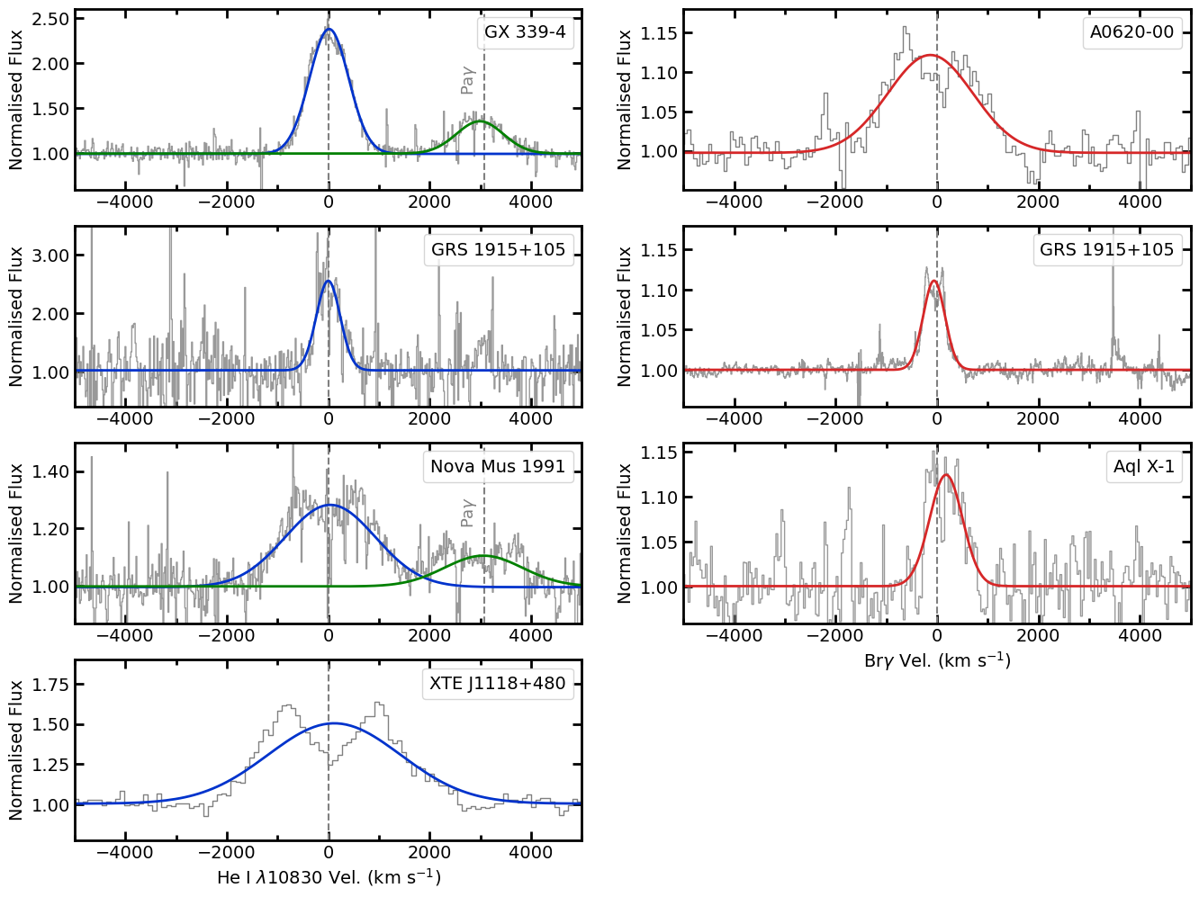
Figure 1: Gaussian fits to the NIR emission line profiles. The left column shows the fits for the He i $\lambda$10830 (blue) and Pa$\gamma$ (green; when the S/N allowed to fit the line) emission lines, while the fits to Br$\gamma$ (red) are shown in the right column.

3 The FWHM-$K_{2}$ correlation

We focused our analysis on the strongest NIR transitions present in the data (He i $\lambda$10830, Pa$\gamma$ and/or Br$\gamma$) using molly and custom software under python 3.7. We carefully normalised each emission line by fitting the adjacent continuum with a low order polynomial and we combined the spectra to obtain one single spectrum per line and source with a higher signal-to-noise ratio (S/N). The FWHM values were obtained from fitting each emission line with a model consisting of a Gaussian profile plus a constant, over a spectral region of $\pm$10000 km s^-1 around the line rest wavelength (with the exception of GRS 1915$+$105, for which we used a spectral region of $\pm$4000 km s^-1 to avoid contamination by nearby instrumental features). We used orthogonal distance regression in the ordinary least squares mode, implementing the python package scipy.odr, to perform these fits. We notice that some of the lines present the double-peaked profile caused by the rotation of the disc (Smak, 1969). However, following Casares (2015), we decided to fit a Gaussian to all the data, which is a more robust model than a double-Gaussian. While the double-Gaussian might fail to fit data of limited spectral resolution and poor S/N, Casares (2015) found that the FWHM values obtained from a single-Gaussian are within a 10$\%$ of those obtained with more complex models. In the case of He i $\lambda$10830, the neighbouring Pa$\gamma$ emission line was masked when present – and vice versa.

Spectral variations from one epoch to another may be present and can be caused by aperiodic flares and orbital changes, such as disc asymmetries (Hynes et al., 2002; Casares, 2015). However, in most cases we are limited by the S/N, which can reflect the observing conditions of the night. In order to estimate the impact of additional systematics related to the intrinsic variability of the FWHM we used the spectra of GX 339-4, which exhibit the highest S/N data in our sample. A Gaussian fit allowed us to estimate the FWHM value of the He i $\lambda$10830  line, along with its corresponding standard deviation, for each of the 16 spectra individually. We then used both the error propagation and the standard deviation to obtain a more conservative error (of $\sim$10$\%$) for the combined data of GX 339-4. Then, for the remaining sources of the sample we estimated the error of the FWHM as the quadratic sum of the statistical error from the fit and the 10$\%$ of the FWHM. To obtain the intrinsic FWHMs, we subtracted the instrumental resolution quadratically. Figure 1 displays the fits to each line included in our sample. In Table 2, we list the FWHM values we measured, as well as the residual variance ($\sigma^{2}_{r}$), which parameterises the quality of the Gaussian fits by quantifying deviations between the data and the best-fitting model, as well the dynamical $K_{2}$ values with their corresponding references. We note that the reported value of $\sigma^{2}_{r}$ for the fit of the He i $\lambda$10830 line in GX 339-4 in Table 2 is an average of the 16 $\sigma^{2}_{r}$ values from the individual fits.

Table 2: SXT parameters.

X-ray transient	Emission	FWHM	$\sigma^{2}_{r}$	$K_{2}$	$K_{2}$ from corr.	Porb	$f(M)$	PMF	Ref.
	line	(km s-1)		(km s-1)	(km s-1)	(days)	($M_{\odot}$)	($M_{\odot}$)
Nova Mus 1991	He i $\lambda$10830	2097 $\pm$ 213	26.07	406.8 $\pm$ 2.7	461 $\pm$ 78	0.43260249(9)	3.02 $\pm$ 0.06	4.4 $\pm$ 2.2	(1)
	Pa$\gamma$	1811 $\pm$ 197	26.06		398 $\pm$ 69			2.8 $\pm$ 1.5
A0620-00	Br$\gamma$	1974 $\pm$ 204	4.31	437.1 $\pm$ 2.0	434 $\pm$ 74	0.32301405(1)	2.79 $\pm$ 0.04	2.7 $\pm$ 1.4	(2)
XTE J1118$+$480	He i $\lambda$10830	3078 $\pm$ 310	20.06	708.8 $\pm$ 1.4	677 $\pm$ 115	0.1699338(5)	6.27 $\pm$ 0.04	5.5 $\pm$ 2.8	(3)
GX 339-4	He i $\lambda$10830	900 $\pm$ 77	4.18	219.0 $\pm$ 3.0	198 $\pm$ 32	1.7587(5)	1.91 $\pm$ 0.08	1.4 $\pm$ 0.7	(4)
	Pa$\gamma$	1088 $\pm$ 111	5.76		239 $\pm$ 41			2.5 $\pm$ 1.3
GRS 1915$+$105	He i $\lambda$10830	551 $\pm$ 59	6.72	126.0 $\pm$ 1.0	121 $\pm$ 21	33.85(16)	7.02 $\pm$ 0.17	6.2 $\pm$ 3.2	(5)
	Br$\gamma$	503 $\pm$ 50	44.34		111 $\pm$ 19			4.8 $\pm$ 2.4
Aql X-1	Br$\gamma$	762 $\pm$ 86	2.45	136.0 $\pm$ 4.0	168 $\pm$ 30	0.7895126(10)	0.21 $\pm$ 0.02	0.4 $\pm$ 0.2	(6)

(1) Wu et al. (2015); (2) González Hernández & Casares (2010); (3) González Hernández et al. (2012); (4) Heida et al. (2017); (5) Steeghs et al. (2013); (6) Mata Sánchez et al. (2017).

In the top panel of Fig. 2, we display the FWHM values versus $K_{2}$ for the SXTs in our sample. A linear fit, using orthogonal distance regression to account for errors in both FWHM and $K_{2}$ values, yields the following relation:

$$K_{2}=0.22(3)\leavevmode\nobreak\ \textrm{FWHM},$$ (1)

where both $K_{2}$ and FWHM are given in km s^-1. The residual variance is $\sigma^{2}_{r}=1.04$. Allowing for a constant term does not improve the fit since it is consistent with zero at 1$\sigma$. We computed the $K_{2}$ values from this relation (see Table 2) and compared them with the dynamical estimations, finding that the differences follow a Gaussian distribution with a standard deviation of 26 km s^-1. We estimated the error of the coefficient in Eq. 1 as the quadratic sum of the statistical error from the fit and the result from a Monte Carlo simulation of 10⁴ events, imposing the condition that the difference between the model and the real $K_{2}$ values follow a Gaussian distribution with $\sigma=26$ km s^-1. It is worth mentioning that although GRS 1915$+$105 was not in full quiescence, and its FWHM values define the bottom end of the correlation, the best-fit parameters remain within the error if we remove those points from the fit.

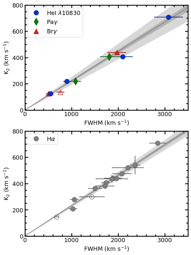
Figure 2: FWHM-$K_{2}$ correlation for SXTs with the best linear fit, using NIR (top panel) and optical (bottom panel; data come from Casares 2015) emission lines. Filled symbols indicate BH binaries, while NS binaries are denoted with open symbols. The shaded regions in both plots correspond to the $1\sigma$ uncertainty of the linear fit (dark grey) and the total uncertainty of the correlation that includes the result from the Monte Carlo simulation in Section 3 (light grey).

Casares (2015) derived an analogous relation in the optical ($K_{2}=0.233(13)$ FWHM) using the FWHM of the H$\alpha$ emission line. We show this data in the bottom panel of Fig. 2. We notice that our NIR correlation (Eq. 1) is fully compatible with that of H$\alpha$. Furthermore, a single fit to the combined H$\alpha$ and NIR FWHM values yields best-fit parameters that are fully consistent with both the optical and NIR correlations.

As explained in Section 3 of Casares (2015), the FWHM-$K_{2}$ correlation is expected from basic equations. Particularly, for BH SXTs with a typical mass ratio $q=0.1$, $K_{2}/\textrm{FWHM}=0.36\sqrt{\alpha}$, where $\alpha$ is the ratio between the disc radius at which the FWHM is determined by gas velocity (R_W) and the effective radius of the compact object’s Roche lobe (R_L1). Our correlation entails that the FWHM of the NIR emission lines trace the disc velocity at 37$\%$ R_L1, implying that these lines are formed in the outer regions of the disc (as is the case for H$\alpha$).

4 Discussion

With the aim of uncovering and studying the reddened population of BHs in the Galaxy, in this work, we compiled the NIR spectra of dynamically studied BH SXTs and a system with a NS during quiescence. We found a correlation between the FWHM of He i $\lambda$10830, Pa$\gamma$, and Br$\gamma$ emission lines, and $K_{2}$ (upper panel in Fig. 2). Despite the low statistics due to the limited availability of NIR spectra of SXTs in quiescence, a comparison with the analogous relation found by Casares (2015) at optical wavelengths, using the H$\alpha$ emission line (bottom panel of Fig. 2), offers evidence of their resemblance, turning the NIR correlation into a reliable tool. Even the correlation of the combined optical and NIR data agrees with the two separate correlations, as mentioned in Section 3.

These correlations allow one to obtain $K_{2}$ by measuring the FWHM in quiescence of either H$\alpha$ or one of the NIR emission lines used in this study. This method only requires one single spectrum with an emission line, which saves considerable observing time when compared to the phase-resolved spectroscopy needed by the classical method (radial velocities) to estimate $K_{2}$. We note, however, that a large orbital coverage would be ideal to avoid potential orbital variations. Nonetheless, an error equal to the quadratic sum of 10% of the FWHM and the statistical error (see Section 3) can be assumed in the FWHM values when a single spectrum is available.

Most importantly, the FWHM-$K_{2}$ correlations are fundamental to uncover the hidden (reddened) population of quiescent BHs in the Galaxy. By combining Eq. 1 with P_orb, we can use Kepler’s third law to estimate a preliminary mass function $\textrm{PMF}=1.1\times 10^{-9}\leavevmode\nobreak\ P_{orb}\leavevmode\nobreak\ \textrm{FWHM}^{3}$, where PMF is in units of $M_{\odot}$, P_orb in days, and FWHM in km s^-1 (see Casares 2015 for the optical analogue). The PMF gives a lower limit to the mass of the compact component in the binary system from single epoch spectroscopy. For PMF $\gtrsim$ 3 M_⊙, the assumed approximate mass limit to segregate BHs from NSs (e.g. Kalogera & Baym, 1996; Rezzolla et al., 2018), we can positively confirm the BH nature of the compact object. Table 2 includes P_orb, as well as our PMF estimations and, for comparison, the dynamical mass functions ($f(M)$) with the corresponding references. As expected, the latter two are fully consistent within the uncertainties.

The similarity of the optical and NIR correlations implies that the widths of H$\alpha$ and the NIR lines, during quiescence, are consistent. This result was expected, since both H$\alpha$ and the NIR emission lines are tracing the velocity from similar outer regions of the disc ($\sim$40$\%$ R_L1; see Section 3). The profiles of spectral disc emission lines from SXTs during outburst have shown both similarities (e.g. between H$\alpha$ and He i $\lambda$10830) and differences (e.g. between Br$\gamma$ with He i $\lambda$10830; Sánchez-Sierras & Muñoz-Darias, 2020) that might be caused by the presence of outflows. In quiescence, however, given the lack of strong accretion activity, we expect the hydrogen and helium transitions to remain mostly unaltered. In the cases were we could measure the width of more than one emission line, we observe that the values are consistent within errors. In order to analyse the correlation for these transitions separately, additional simultaneous data are required.

Using a sample of cataclysmic variables, Casares (2015) showed that the slope of the FWHM-$K_{2}$ correlation decreases with increasing mass ratio q. We note that one of our systems, Aql X-1, is a NS SXT with $q=0.41\pm 0.08$ (Mata Sánchez et al., 2017), while the others are BH SXTs with typical mass ratios $q\sim 0.1$. This may explain why Aql X-1 lies slightly under the correlation in Fig. 2. However, a single data point is not enough to make strong assumptions, and more observations of NS SXTs are needed for confirmation.

Following with exploiting relations to derive fundamental parameters from faint SXTs, future work should employ NIR emission lines to explore the correlations previously established using H$\alpha$. In particular, Casares (2016) reported a correlation between the mass ratio (q) and the ratio of the double-peaked separation to the FWHM of H$\alpha$. Subsequently, a correlation between the binary inclination and the depth of the trough from the double-peaked H$\alpha$ was presented by Casares et al. (2022).

5 Conclusions

In this work, we compiled quiescent NIR spectra of SXTs —mainly BHs— with known $K_{2}$ values, and measured the FWHM of He i $\lambda$10830, Pa$\gamma$ and/or Br$\gamma$ emission lines. We present a NIR FWHM-$K_{2}$ correlation that allow us to estimate $K_{2}$ of faint SXTs from single-epoch spectroscopy, saving substantial observing time when compared to the phase-resolved radial velocity method. We find that this NIR correlation is fully consistent with its optical analogue. This result, together with the similarity of the FWHM values of different NIR lines in a given system, suggests that any H or He i transition could be useful for estimating $K_{2}$. Most importantly, we are then able to constrain the mass function of the compact object in the system by combining the FWHM-$K_{2}$ relation with P_orb. This new NIR correlation will not only reveal the nature of highly-reddened SXTs, but will also expand the Galactic BH statistics, allowing for detailed studies of their formation mechanisms.

References

- Abbott et al. (2023) Abbott, R., Abbott, T. D., Acernese, F., et al. 2023, Physical Review X, 13, 46
- Astropy Collaboration et al. (2018) Astropy Collaboration, Price-Whelan, A. M., Sipőcz, B. M., et al. 2018, AJ, 156, 123
- Astropy Collaboration et al. (2013) Astropy Collaboration, Robitaille, T. P., Tollerud, E. J., et al. 2013, A&A, 558, 33
- Belczynski et al. (2012) Belczynski, K., Wiktorowicz, G., Fryer, C. L., Holz, D. E., & Kalogera, V. 2012, ApJ, 757, 91
- Casares (2015) Casares, J. 2015, ApJ, 808, 80
- Casares (2016) Casares, J. 2016, ApJ, 822, 99
- Casares (2018) Casares, J. 2018, MNRAS, 473, 5195
- Casares et al. (1992) Casares, J., Charles, P. A., & Naylor, T. 1992, Nature, 355, 614
- Casares & Jonker (2014) Casares, J. & Jonker, P. G. 2014, Space Science Reviews, 183, 223
- Casares et al. (2017) Casares, J., Jonker, P. G., & Israelian, G. 2017, in Handbook of Supernovae (Springer International Publishing), 1499–1526
- Casares et al. (2022) Casares, J., Muñoz-Darias, T., Torres, M. A. P., et al. 2022, MNRAS, 516, 2023
- Charles & Coe (2006) Charles, P. A. & Coe, M. J. 2006, in Compact stellar X-ray sources, ed. W. Lewin & M. van der Klis (Cambridge Astrophysics Series, No. 39. Cambridge, UK: Cambridge University Press), 215 – 265
- Corral-Santana et al. (2016) Corral-Santana, J. M., Casares, J., Muñoz-Darias, T., et al. 2016, A&A, 587, 61
- Corral-Santana et al. (2011) Corral-Santana, J. M., Casares, J., Shahbaz, T., et al. 2011, MNRAS, 413, L15
- El-Badry et al. (2023) El-Badry, K., Rix, H. W., Cendes, Y., et al. 2023, MNRAS, 521, 4323
- Fabian (2012) Fabian, A. C. 2012, ARA&A, 50, 455
- Fender & Muñoz-Darias (2016) Fender, R. & Muñoz-Darias, T. 2016, in Lecture Notes in Physics, Vol. 905 (Springer Verlag), 65–100
- Giesers et al. (2018) Giesers, B., Dreizler, S., Husser, T. O., et al. 2018, MNRAS, 475, L15
- González Hernández & Casares (2010) González Hernández, J. I. & Casares, J. 2010, A&A, 516, 58
- González Hernández et al. (2012) González Hernández, J. I., Rebolo, R., & Casares, J. 2012, ApJ, 744, L25
- González Hernández et al. (2017) González Hernández, J. I., Suárez-Andrés, L., Rebolo, R., & Casares, J. 2017, MNRAS, 465, L15
- Harris et al. (2020) Harris, C. R., Millman, K. J., van der Walt, S. J., et al. 2020, Nature, 585, 357
- Harrison et al. (2007) Harrison, T. E., Howell, S. B., Szkody, P., & Cordova, F. A. 2007, AJ, 133, 162
- Heida et al. (2017) Heida, M., Jonker, P. G., Torres, M. A. P., & Chiavassa, A. 2017, ApJ, 846, 132
- Hunter (2007) Hunter, J. D. 2007, Computing in Science & Engineering, 9, 90
- Hynes et al. (2002) Hynes, R. I., Zurita, C., Haswell, C. A., et al. 2002, MNRAS, 330, 1009
- Kalogera & Baym (1996) Kalogera, V. & Baym, G. 1996, ApJ, 470, L61
- Khargharia et al. (2013) Khargharia, J., Froning, C. S., Robinson, E. L., & Gelino, D. M. 2013, AJ, 145, 21
- Kiel & Hurley (2006) Kiel, P. D. & Hurley, J. R. 2006, MNRAS, 369, 1152
- Lam et al. (2022) Lam, C. Y., Lu, J. R., Udalski, A., et al. 2022, ApJ, 933, L23
- Mata Sánchez et al. (2015) Mata Sánchez, D., Muñoz-Darias, T., Casares, J., Corral-Santana, J. M., & Shahbaz, T. 2015, MNRAS, 454, 2199
- Mata Sánchez et al. (2017) Mata Sánchez, D., Muñoz-Darias, T., Casares, J., & Jiménez-Ibarra, F. 2017, MNRAS, 464, 41
- McClintock & Remillard (2006) McClintock, J. E. & Remillard, R. A. 2006, in Compact Stellar X-ray Sources (Cambridge University Press), 157–214
- Motta et al. (2021) Motta, S. E., Kajava, J. J., Giustini, M., et al. 2021, MNRAS, 503, 152
- Reynolds (2021) Reynolds, C. S. 2021, ARA&A, 59, 117
- Rezzolla et al. (2018) Rezzolla, L., Most, E. R., & Weih, L. R. 2018, ApJ, 852, L25
- Romani (1998) Romani, R. W. 1998, A census of low mass black hole binaries, Tech. rep.
- Sahu et al. (2022) Sahu, K. C., Anderson, J., Casertano, S., et al. 2022, ApJ, 933, 83
- Sánchez-Sierras & Muñoz-Darias (2020) Sánchez-Sierras, J. & Muñoz-Darias, T. 2020, A&A, 640
- Smak (1969) Smak, J. 1969, Acta Astron., 19, 155
- Steeghs et al. (2013) Steeghs, D., Mcclintock, J. E., Parsons, S. G., et al. 2013, ApJ, 768, 185
- Tetarenko et al. (2016) Tetarenko, B. E., Sivakoff, G. R., Heinke, C. O., & Gladstone, J. C. 2016, ApJS, 222, 15
- Tody (1986) Tody, D. 1986, in Instrumentation in Astronomy VI, Vol. 0627 (SPIE), 733
- Torres et al. (2019) Torres, M. A. P., Casares, J., Jiménez-Ibarra, F., et al. 2019, ApJ, 882, L21
- Virtanen et al. (2020) Virtanen, P., Gommers, R., Oliphant, T. E., et al. 2020, Nature Methods, 17, 261
- Wang & Chen (2019) Wang, S. & Chen, X. 2019, ApJ, 877, 116
- Wu et al. (2015) Wu, J., Orosz, J. A., McClintock, J. E., et al. 2015, ApJ, 806, 92
- Yanes-Rizo et al. (2022) Yanes-Rizo, I. V., Torres, M. A. P., Casares, J., et al. 2022, MNRAS, 517, 1476
- Yungelson et al. (2006) Yungelson, L. R., Lasota, J.-P., Nelemans, G., et al. 2006, A&A, 454, 559