Counterfactual Fairness for Predictions using Generative Adversarial Networks

Abstract

Fairness in predictions is of direct importance in practice due to legal, ethical, and societal reasons. It is often achieved through counterfactual fairness, which ensures that the prediction for an individual is the same as that in a counterfactual world under a different sensitive attribute. However, achieving counterfactual fairness is challenging as counterfactuals are unobservable. In this paper, we develop a novel deep neural network called Generative Counterfactual Fairness Network (GCFN) for making predictions under counterfactual fairness. Specifically, we leverage a tailored generative adversarial network to directly learn the counterfactual distribution of the descendants of the sensitive attribute, which we then use to enforce fair predictions through a novel counterfactual mediator regularization. If the counterfactual distribution is learned sufficiently well, our method is mathematically guaranteed to ensure the notion of counterfactual fairness. Thereby, our GCFN addresses key shortcomings of existing baselines that are based on inferring latent variables, yet which (a) are potentially correlated with the sensitive attributes and thus lead to bias, and (b) have weak capability in constructing latent representations and thus low prediction performance. Across various experiments, our method achieves state-of-the-art performance. Using a real-world case study from recidivism prediction, we further demonstrate that our method makes meaningful predictions in practice.

1 Introduction

Fairness in machine learning is mandated for a large number of practical applications due to legal, ethical, and societal reasons (Angwin et al., 2016; Barocas & Selbst, 2016; De Arteaga et al., 2022; Feuerriegel et al., 2020; Kleinberg et al., 2019; von Zahn et al., 2022). Examples are predictions in credit lending or recidivism prediction, where fairness is mandated by anti-discrimination laws.

In this paper, we focus on the notion of counterfactual fairness (Kusner et al., 2017). The notion of counterfactual fairness has recently received significant attention (e.g., Abroshan et al., 2022; Garg et al., 2019; Grari et al., 2023; Kim et al., 2021; Kusner et al., 2017; Ma et al., 2023; Xu et al., 2019). One reason is that counterfactual fairness directly relates to legal terminology in that a prediction is fair towards an individual if the prediction does not change had the individual belonged to a different demographic group defined by some sensitive attribute (e.g., gender, race). However, ensuring counterfactual fairness is challenging as, in practice, counterfactuals are generally unobservable.

Prior works have developed methods for achieving counterfactual fairness in predictive tasks (see Sec. 2). Originally, Kusner et al. (2017) described a conceptual algorithm to achieve counterfactual fairness. Therein, the idea is to first estimate a set of latent (background) variables and then train a prediction model without using the sensitive attribute or its descendants. More recently, the conceptual algorithm has been extended through neural methods, where the latent variables are learned using variational autoencoders (VAEs) (Grari et al., 2023; Kim et al., 2021; Pfohl et al., 2019). However, these methods have key shortcomings: (a) the learned representation can be potentially correlated with the sensitive attributes, which thus leads to bias, and (b) VAEs have weak capability in constructing latent representations, which leads to a low prediction performance. We address both shortcomings (a) and (b) in our proposed method through the theoretical properties of our counterfactual mediator regularization and our tailored GAN, respectively.

In this paper, we present a novel deep neural network called Generative Counterfactual Fairness Network (GCFN) for making predictions under counterfactual fairness. Our method leverages a tailored generative adversarial network to directly learn the counterfactual distribution of the descendants of the sensitive attribute. We then use the generated counterfactuals to enforce fair predictions through a novel counterfactual mediator regularization. We show theoretically: if the counterfactual distribution is learned sufficiently well, our method is guaranteed to ensure the notion of counterfactual fairness.

Overall, our main contributions are as follows: (1) We propose a novel deep neural network for achieving counterfactual fairness in predictions, which addresses key limitations of existing baselines. (2) We further show that, if the counterfactual distribution is learned sufficiently well, our method is guaranteed to ensure counterfactual fairness. (3) We demonstrate that our GCFN achieves the state-of-the-art performance. We further provide a real-world case study of recidivism prediction to show that our method gives meaningful predictions in practice.

2 Related work

Several research streams are relevant to our work, and we briefly discuss them in the following: (1) fairness notions for predictions, (2) methods for counterfactual fairness, (3) generative models for fair synthetic datasets, and (4) generative models for estimating causal effects.

Fairness notions for predictions: Over the past years, the machine learning community has developed an extensive series of fairness notions for predictive tasks so that one can train unbiased machine learning models; see Appendix B for a detailed overview. In this paper, we focus on counterfactual fairness (Kusner et al., 2017), due to its relevance in practice (Barocas & Selbst, 2016; De Arteaga et al., 2022).

Predictions under counterfactual fairness: Originally, Kusner et al. (2017) introduced a conceptual algorithm to achieve predictions under counterfactual fairness. The idea is to first infer a set of latent background variables and subsequently train a prediction model using these inferred latent variables and non-descendants of sensitive attributes. However, the conceptual algorithm requires knowledge of the ground-truth structural causal model, which makes it impractical.

State-of-the-art approaches build upon the above idea but integrate neural learning techniques, typically by using VAEs. These are mCEVAE (Pfohl et al., 2019), DCEVAE (Kim et al., 2021), and ADVAE (Grari et al., 2023). In general, these methods proceed by first computing the posterior distribution of the latent variables, given the observational data and a prior on latent variables. Based on that, they compute the implied counterfactual distributions, which can either be utilized directly for predictive purposes or can act as a constraint incorporated within the training loss. Further details are in Appendix B. In sum, the methods in Grari et al. (2023); Kim et al. (2021); Pfohl et al. (2019) are our main baselines.

However, the above methods have two main shortcomings. (a) The inferred latent variables can be potentially correlated with sensitive attributes because some information from sensitive attributes can leak into latent variables. This could introduce bias in the prediction. (b) It is commonly assumed that the prior distribution of latent variables follows a standard Gaussian in VAEs. However, this might be inadequate for capturing complex distributions, potentially leading to imprecise approximations of counterfactual distributions and thus overall low prediction performance. In our method, we later address (a) through the theoretical properties of our counterfactual mediator regularization and (b) through our tailored GAN.

Generating fair synthetic datasets: A different literature stream has used generative models to create fair synthetic datasets (e.g., van Breugel et al., 2021; Xu et al., 2018; Rajabi & Garibay, 2022; Xu et al., 2019). Importantly, the objective here is different from ours, namely, predictions under counterfactual fairness. Still, one could potentially adapt these methods to our task by first learning a fair dataset and then training a prediction model. We thus later adapt the procedure for our evaluation. Several methods focus on fairness notions outside of counterfactual fairness and are thus not applicable. We are only aware of one method called CFGAN (Xu et al., 2019) which is aimed at counterfactual fairness, and we later use it as a baseline. While CFGAN also employs GANs, its architecture is vastly different from our method. Besides, CFGAN uses the GAN to generate entirely synthetic data, while we use the GAN to generate counterfactuals of the mediator (see Appendix B for details). Moreover, baselines based on fair synthetic datasets have crucial limitations for our task: they learn the predictions not from the original but from the transformed dataset, which leads to information loss and thus a low prediction performance.

Deep generative models for estimating causal effects: There are many papers that leverage generative adversarial networks and variational autoencoders to estimate causal effects from observational data (Kocaoglu et al., 2018; Louizos et al., 2017; Pawlowski et al., 2020; Yoon et al., 2018; Bica et al., 2020). We later borrow some ideas of modeling counterfactuals through deep generative models, yet we emphasize that those methods aim at estimating causal effects but without fairness considerations.

Research gap: Existing baselines that are based on inferring latent variables, can have the problems that latent variables are potentially correlated with the sensitive attributes and thus lead to bias and that have weak capability in constructing latent representations and thus low prediction performance. As a remedy, we develop a novel deep neural network called Generative Counterfactual Fairness Network (GCFN) that addresses those shortcomings. We directly learn the counterfactual distribution through a tailored generative adversarial network and enforce counterfactual fairness through a novel counterfactual mediator regularization.

3 Problem Setup

Notation: Capital letters such as $X,A,M$ denote random variables and small letters $x,a,m$ denote their realizations from corresponding domains $\mathcal{X},\mathcal{A},\mathcal{M}$. Further, $\mathbb{P}(M)=\mathbb{P}_{M}$ is the probability distribution of $M$; $\mathbb{P}(M\mid$ $A=a$ ) is a conditional (observational) distribution; $\mathbb{P}\left(M_{a}\right)$ the interventional distribution on $M$ when setting $A$ to $a$; and $\mathbb{P}\left(M_{a^{\prime}}\mid A=a,M=m\right)$ the counterfactual distribution of $M$ had $A$ been set to $a^{\prime}$ given evidence $A=a$ and $M=m$.

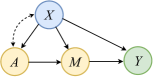
Figure 1: Causal graph. The nodes represent: sensitive attribute, $A$; covariate, $X$; mediator, $M$; target, $Y$. $\longrightarrow$ represents direct causal effect; $\dashleftarrow\dashrightarrow$ represents potential presence of hidden confounders.

Our causal graph is shown in Fig 1, where the nodes represent: sensitive attribute $A\in\mathcal{A}$; mediators $M\in\mathcal{M}$, which are possibly causally influenced by the sensitive attribute; covariates $X\in\mathcal{X}$, which are not causally influenced by the sensitive attribute; and a target $Y\in\mathcal{Y}$. In our setting, $A$ can be a categorical variable with multiple categories $k$ and $X$ and $M$ can be multi-dimensional. For ease of notation, we use $k=2$, i.e., $\mathcal{A}=\{0,1\}$, to present our method below.

We use the potential outcomes framework (Rubin, 1974) to estimate causal quantities from observational data. Under our causal graph, the dependence of $M$ on $A$ implies that changes in the sensitive attribute $A$ mean also changes in the mediator $M$. We use subscripts such as $M_{a}$ to denote the potential outcome of $M$ when intervening on $A$. Similarly, $Y_{a}$ denotes the potential outcome of $Y$. Furthermore, for $k=2$, $A$ is the factual and $A^{\prime}$ is the counterfactual outcome of the sensitive attribute.

In practice, it is common and typically straightforward to choose which variables act as mediators $M$ through domain knowledge Nabi & Shpitser (2018); Kim et al. (2021); Plecko & Bareinboim (2022). Hence, mediators $M$ are simply all variables that can potentially be influenced by the sensitive attribute. All other variables (except for $A$ and $Y$) are modeled as the covariates $X$. For example, consider a job application setting where we want to avoid discrimination by gender. Then $A$ is gender, and $Y$ is the job offer. Mediators are, for instance, education level or work experience, as both are potentially influenced by gender. In contrast, age is a covariate because it is not influenced by gender.

Our model follows standard assumptions necessary to identify causal queries (Rubin, 1974). (1) Consistency: The observed mediator is identical to the potential mediator given a certain sensitive attribute. Formally, for each unit of observation, $A=a\Rightarrow M=M_{a}$. (2) Overlap: For all ${x}$ such that $\mathbb{P}(X={x})>0$, we have $0<\mathbb{P}\left(A={a}\mid X={x}\right)<1$, $\forall{a}\in\mathcal{A}$. (3) Unconfoundedness: Conditional on covariates $X$, the potential outcome $M_{a}$ is independent of sensitive attribute $A$, i.e. $M_{a}\perp\!\!\!\perp A\mid X$.

Objective: In this paper, we aim to learn the prediction of a target $Y$ to be counterfactual fair with respect to some given sensitive attribute $A$ so that it thus fulfills the notion of counterfactual fairness (Kusner et al., 2017). Let $h(X,M)=\hat{Y}$ denote the predicted target from some prediction model, which only depends on covariates and mediators. Formally, our goal is to have $h$ achieve counterfactual fairness if under any context $X={x}$, $A={a}$, and $M={m}$, that is,

$$\mathbb{P}\left(h(x,M_{a})\mid X={x},A=a,M={m}\right)=\mathbb{P}\left(h(x,M_{a^{\prime}})\mid X={x},A=a,M={m}\right).$$ (1)

This equation illustrates the need to care about the counterfactual mediator distribution. Under the consistency assumption, the right side of the equality simplifies to the delta (point mass) distribution $\delta\left({h(x,m)}\right)$.

4 Generative Counterfactual Fairness Network

Overview: Here, we introduce our proposed method called Generative Counterfactual Fairness Network (GCFN). An overview of our method is in Fig. 2. GCFN proceeds in two steps: Step 1 uses a significantly modified GAN to learn the counterfactual distribution of the mediator. Step 2 uses the generated counterfactual mediators from the first step together with our counterfactual mediator regularization to enforce counterfactual fairness. The pseudocode is in Appendix C.

Why do we need counterfactuals of the mediator? Different from existing methods for causal effect estimation (Bica et al., 2020; Yoon et al., 2018), we are not interested in obtaining counterfactuals of the target $Y$. Instead, we are interested in counterfactuals for the mediator $M$, which captures the entire influence of the sensitive attribute and its descendants on the target. Thus, by training the prediction model with our counterfactual mediator regularization, we remove the information from the sensitive attribute to ensure fairness while keeping the rest useful information of data to maintain high prediction performance.

What is the advantage of using a GAN in our method? The GAN in our method enables us to directly learn transformations of factual mediators to counterfactuals without the need for fitting an explicit probabilistic model, such as variational autoencoders (VAEs) or normalizing flows (NFs). As a result, we eliminate the need for the abduction-action-prediction procedure (Pearl, 2009) that is common in the baselines for inferring latent variables, which can be very challenging for high-dimensional data.

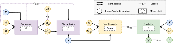
Figure 2: Overview of our GCFN for achieving counterfactual fairness in predictions. Step 1: The generator $G$ takes $\left(X,A,M\right)$ as input and outputs $\hat{M}_{A}$ and $\hat{M}_{A^{\prime}}$. The discriminator ${D}$ differentiates the observed factual mediator ${M}$ from the generated counterfactual mediator $\hat{M}_{A^{\prime}}$. Step 2: We then use generated counterfactual mediator $\hat{M}_{A^{\prime}}$ in our counterfactual mediator regularization $\mathcal{R}_{\mathrm{{cm}}}$. The counterfactual mediator regularization $\mathcal{R}_{\mathrm{{cm}}}$ enforces the prediction model $h$ to be counterfactual fairness.

4.1 Step 1: GAN for generating counterfactual of the mediator

In Step 1, we aim to generate counterfactuals of the mediator (since the ground-truth counterfactual mediator is unavailable). Our generator ${G}$ produces the counterfactual of the mediators given observational data. Concurrently, our discriminator ${D}$ differentiates the factual mediator from the generated counterfactual mediators. This adversarial training process encourages ${G}$ to learn the counterfactual distribution of the mediator.

4.1.1 Counterfactual generator $G$

The objective of the generator $G$ is to learn the counterfactual distribution of the mediator, i.e., $\mathbb{P}\left({M}_{a^{\prime}}\mid X=x,A=a,M=m\right)$. Formally, $G:\mathcal{X}\times\mathcal{A}\times\mathcal{M}\rightarrow\mathcal{M}$. ${G}$ takes the factual sensitive attribute $A$, the factual mediator $M$, and the covariates $X$ as inputs, sampled from the joint (observational) distribution $\mathbb{P}_{X,A,M}$, denoted as $\mathbb{P}_{\mathrm{f}}$ for short. $G$ outputs two potential mediators, $\hat{M}_{0}$ and $\hat{M}_{1}$, from which one is factual and the other is counterfactual. For notation, we use $G\left(X,A,M\right)$ to refer to the output of the generator. Thus, we have

$${G}\left(X,A,M\right)_{a}=\hat{M}_{a}\quad\text{for}\quad a\in\{0,1\}$$ (2)

In our generator $G$, we intentionally output not only the counterfactual mediator but also the factual mediator, even though the latter is observable. The reason is that we can use it to further stabilize the training of the generator. For this, we introduce a reconstructive loss $\mathcal{L}_{\mathrm{f}}$, which we use to ensure that the generated factual mediator $\hat{M}_{A}$ is similar to the observed factual mediator $M$. Formally, we define the reconstruction loss

$$\mathcal{L}_{\mathrm{f}}(G)=\mathbb{E}_{({X,A,M)\sim\mathbb{P}_{\mathrm{f}}}}\left[\left\|M-{G}\left(X,A,M\right)_{A}\right\|^{2}_{2}\right],$$ (3)

where $\|\cdot\|_{2}$ is the $L_{2}$-norm.

4.1.2 Counterfactual discriminator $D$

The discriminator $D$ is carefully adapted to our setting. In an ideal world, we would have $D$ discriminate between real vs. fake counterfactual mediators; however, the counterfactual mediators are not observable. Instead, we train $D$ to discriminate between factual mediators vs. generated counterfactual mediators. Note that this is different from the conventional discriminators in GANs that seek to discriminate real vs. fake samples (Goodfellow et al., 2014a). Formally, our discriminator ${D}$ is designed to differentiate the factual mediator $M$ (as observed in the data) from the generated counterfactual mediator $\hat{M}_{A^{\prime}}$ (as generated by $G$).

We modify the output of $G$ before passing it as input to $D$: We replace the generated factual mediator $\hat{M}_{A}$ with the observed factual mediator $M$. We denote the new, combined data by $\tilde{G}\left(X,A,M\right)$, which is defined via

$$\tilde{G}\left(X,A,M\right)_{a}=\begin{cases}{M},&\text{if }A=a,\\ {G}\left(X,A,M\right)_{a},&\text{if }A=a^{\prime},\end{cases}\quad\text{for }a\in\{0,1\}.$$ (4)

The discriminator ${D}$ then determines which component of $\tilde{G}$ is the observed factual mediator and thus outputs the corresponding probability. Formally, for the input $(X,\tilde{G})$, the output of the discriminator $D$ is

$${D}\left(X,\tilde{G}\right)_{a}=\hat{\mathbb{P}}\left(M=\tilde{G}_{a}\mid X,\tilde{G}\right)=\hat{\mathbb{P}}\left(A=a\mid X,\tilde{G}\right)\quad\text{for }a\in\{0,1\}.$$ (5)

4.1.3 Adversarial training of our GAN

Our GAN is trained in an adversarial manner: (i) the generator ${G}$ seeks to generate counterfactual mediators in a way that minimizes the probability that the discriminator can differentiate between factual mediators and counterfactual mediators, while (ii) the discriminator $D$ seeks to maximize the probability of correctly identifying the factual mediator. We thus use an adversarial loss $\mathcal{L}_{\mathrm{adv}}$ by

$$\mathcal{L}_{\mathrm{adv}}(G,D)=\mathbb{E}_{({X,A,M)\sim\mathbb{P}_{\mathrm{f}}}}\left[\log\big{(}{D}(X,\tilde{G}\left(X,A,M\right))_{A}\big{)}\right].$$ (6)

Overall, our GAN is trained through an adversarial training procedure with a minimax problem as

$$\min_{G}\max_{D}\mathcal{L}_{\mathrm{adv}}(G,D)+\alpha\mathcal{L}_{\mathrm{f}}(G),$$ (7)

with a hyperparameter $\alpha$ on $\mathcal{L}_{\mathrm{f}}$. We show in Appendix D that, under mild identifiability conditions, the counterfactual distribution of the mediator, i.e., $\mathbb{P}\left({M}_{a^{\prime}}\mid X=x,A=a,M=m\right)$, is consistently estimated by our GAN.

4.2 Step 2: Counterfactual fair prediction through counterfactual mediator regularization

In Step 2, we use the output of the GAN to train a prediction model under counterfactual fairness in a supervised way. For this, we introduce our counterfactual mediator regularization that enforces counterfactual fairness w.r.t the sensitive attribute. Let $h$ denote our prediction model (e.g., a neural network). We define our counterfactual mediator regularization $\mathcal{R}_{\mathrm{{cm}}}(h)$ as

$$\mathcal{R}_{\mathrm{{cm}}}(h)=\mathbb{E}_{({X,A,M)\sim\mathbb{P}_{\mathrm{f}}}}\left[\left\|h\left(X,M\right)-h\left(X,\hat{M}_{A^{\prime}}\right)\right\|^{2}_{2}\right].$$ (8)

Our counterfactual mediator regularization has three important characteristics: (1) It is non-trivial. Different from traditional regularization, our $\mathcal{R}_{\mathrm{{cm}}}$ is not based on the representation of the prediction model $h$ but it involves a GAN-generated counterfactual $\hat{M}_{A^{\prime}}$ that is otherwise not observable. (2) Our $\mathcal{R}_{\mathrm{{cm}}}$ is not used to constrain the learned representation (e.g., to avoid overfitting) but it is used to change the actual learning objective to achieve the property of counterfactual fairness. (3) Our $\mathcal{R}_{\mathrm{{cm}}}$ fulfills theoretical properties (see Sec. 4.3). Specifically, we show later that, under some conditions, our regularization actually optimizes against counterfactual fairness and thus should learn our task as desired.

The overall loss $\mathcal{L}(h)$ is as follows. We fit the prediction model $h$ using a cross-entropy loss $\mathcal{L}_{\mathrm{ce}}(h)$. We further integrate the above counterfactual mediator regularization $\mathcal{R}_{\mathrm{{cm}}}(h)$ into our overall loss $\mathcal{L}(h)$. For this, we introduce a weight $\lambda\geq 0$ to balance the trade-off between prediction performance and the level of counterfactual fairness. Formally, we have

$$\mathcal{L}(h)=\mathcal{L}_{\mathrm{ce}}(h)+\lambda\mathcal{R}_{\mathrm{{cm}}}(h).$$ (9)

A large value of $\lambda$ increases the weight of $\mathcal{R}_{\mathrm{{cm}}}$, thus leading to a prediction model that is strict with regard to counterfactual fairness, while a lower value allows the prediction model to focus more on producing accurate predictions. As such, $\lambda$ offers additional flexibility to decision-makers as they tailor the prediction model based on the fairness needs in practice.

4.3 Theoretical insights

Below, we provide theoretical insights to show that our proposed counterfactual mediator regularization is effective in ensuring counterfactual fairness for predictions. Following Grari et al. (2023), we measure the level of counterfactual fairness through $\mathit{CF}$ computed via $\mathbb{E}\left[\left\|\left(h\left(X,M\right)-h\left(X,M_{A^{\prime}}\right)\right)\right\|^{2}_{2}\right]$. It is straightforward to see that, the smaller $\mathit{CF}$ is, the more counterfactual fairness the prediction model achieves.

We now show that, by empirically measuring our generated counterfactual of the mediator, we can thus quantify to what extent counterfactual fairness $\mathit{CF}$ is fulfilled in the prediction model. We give an upper bound in the following lemma.

Lemma 1 (Counterfactual mediator regularization bound).

Given the prediction model $h$ that is Lipschitz continuous with a Lipschitz constant $\mathcal{C}$, we have

$$\mathbb{E}\left[\left\|(h(X,M)-h(X,M_{A^{\prime}})\right\|^{2}_{2}\right]\leq\mathcal{C}\,\mathbb{E}\left[\left\|M_{A^{\prime}}-\hat{M}_{A^{\prime}}\right\|^{2}_{2}\right]+\mathcal{R}_{\mathrm{{cm}}}(h).$$ (10)

Proof.

See Appendix D. ∎

The inequality in Lemma 1 states that the influence from the sensitive attribute on the target variable is upper-bounded by: (i) the performance of generating the counterfactual of the mediator (first term) and (ii) the counterfactual mediator regularization (second term). Hence, by reducing the counterfactual mediator regularization $\mathcal{R}_{\mathrm{{cm}}}$, we effectively enforce the prediction to be more counterfactual fair if the performance generating the counterfactual of the mediator (first term) is sufficiently good. In other words, if the counterfactual distribution is learned sufficiently well, our method is mathematically guaranteed to ensure the notion of counterfactual fairness. We also provide guarantees for estimating the counterfactual distribution in Appendix D.

5 Experiments

5.1 Setup

Baselines: We compare our method against the following state-of-the-art approaches: (1) CFAN (Kusner et al., 2017): Kusner et al.’s algorithm with additive noise where only non-descents of sensitive attributes and the estimated latent variables are used for prediction; (2) CFUA (Kusner et al., 2017): a variant of the algorithm which does not use the sensitive attribute or any descents of the sensitive attribute; (3) mCEVAE (Pfohl et al., 2019): adds a maximum mean discrepancy to regularize the generations in order to remove the information the inferred latent variable from sensitive information; (4) DCEVAE (Kim et al., 2021): a VAE-based approach that disentangles the exogenous uncertainty into two variables; (5) ADVAE (Grari et al., 2023): adversarial neural learning approach which should be more powerful than penalties from maximum mean discrepancy but is aimed the continuous setting; (6) HSCIC (Quinzan et al., 2022): originally designed to enforces the predictions to remain invariant to changes of sensitive attributes using conditional kernel mean embeddings but which we adapted for counterfactual fairness. We also adapt applicable baselines from fair dataset generation: (7) CFGAN (Xu et al., 2019): which we extend with a second-stage prediction model. Details are in Appendix F.

Performance metrics: Methods for causal fairness aim at both: (i)  achieve high accuracy while (ii) ensuring causal fairness, which essentially yields a multi-criteria decision-making problem. To this end, we follow standard procedures and reformulate the multi-criteria decision-making problem using a utility function $U_{\gamma}(\mathit{accuracy},\mathit{CF}):\mathbb{R}^{2}\mapsto\mathbb{R}$, where $\mathit{CF}$ is the metric for measuring counterfactual fairness from Sec. 4.3. We define the utility function as $U_{\gamma}(\mathit{accuracy},\mathit{CF})=\mathit{accuracy}-\gamma\times\mathit{CF}$ with a given utility weight $\gamma$. A larger utility $U_{\gamma}$ is better. The weight $\gamma$ depends on the application and is set by the decision-maker; here, we report results for a wide range of weights $\gamma\in\{0.1,\ldots,1.0\}$.

Implementation details: We implement our GCFN in PyTorch. Both the generator and the discriminator are designed as deep neural networks. We use LeakyReLU, batch normalization in the generator for stability, and train the GAN for $300$ epochs with $256$ batch size. The prediction model is a multilayer perceptron, which we train for $30$ epochs at a $0.005$ learning rate. Since the utility function considers two metrics, the weight $\lambda$ is set to $0.5$ to get a good balance. More implementation details and hyperparameter tuning are in Appendix F.

5.2 Results for (semi-)synthetic datasets

We explicitly focus on (semi-)synthetic datasets, which allow us to compute the true counterfactuals and thus validate the effectiveness of our method.

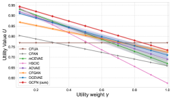
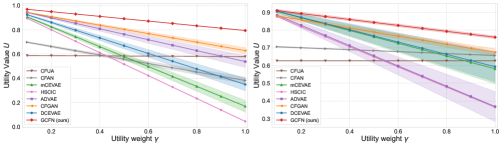
Figure 3: Results for (semi-)synthetic datasets. Left: fully-synthetic dataset. Center: semi-synthetic dataset with sigmoid function. Right: with $\sin$ function. A larger utility is better. Shown: mean $\pm$ std over 5 runs.

Setting: (1) We follow previous works that simulate a fully synthetic dataset for performance evaluations (Kim et al., 2021; Quinzan et al., 2022). We simulate sensitive attributes and target to follow a Bernoulli distribution with the sigmoid function while the mediator is generated from a function of the sensitive attribute, covariates, and some Gaussian noise. (2) We use the Law School (Wightman, 1998) dataset to predict whether a candidate passes the bar exam and where gender is the sensitive attribute. The mediator uses a linear combination together with a sigmoid function. The target variable is generated from the Bernoulli distribution with a probability calculated by a function of covariates, mediator, and noise. (3) We follow the previous dataset but, instead of a sigmoid function, we generate the mediator via a $\sin$ function. The idea behind this is to have a more flexible data-generating function, which makes it more challenging to learn latent variables. For all datasets, we use 20% as a test set. Further details are in Appendix E.

Results: Results are shown in Fig. 3. We make the following findings. (1) Our GCFN performs best. (2) Compared to the baselines, the performance gain from our GCFN is large (up to $\sim$30%). (3) The performance gain for our GCFN tends to become larger for larger $\gamma$. (4) Most baselines in the semi-synthetic dataset with sin function have a large variability across runs as compared to our GCFN, which further demonstrates the robustness of our method. (5) Conversely, the strong performance of our GCFN in the semi-synthetic dataset with sin function demonstrates that our tailed GAN can even capture complex counterfactual distributions.

Table 1: Our GCFN can learn the distribution of the counterfactual mediator. The normalized MSE($M_{A^{\prime}}$,$\hat{M}_{A^{\prime}}$) is $\approx 0$, showing the generated counterfactual mediator is similar to the ground-truth counterfactual mediator. In contrast, both the factual and the generated counterfactual mediator are highly dissimilar.

	Synthetic	Semi-syn. (sigmoid)	Semi-syn. (sin)
MSE($M$, $M_{A^{\prime}}$)	1.00$\pm$0.00	1.00$\pm$0.00	1.00$\pm$0.00
MSE($M$, $\hat{M}_{A^{\prime}}$)	1.00$\pm$0.005	1.00$\pm$0.003	1.01$\pm$0.004
MSE($M_{A^{\prime}}$, $\hat{M}_{A^{\prime}}$)	0.01$\pm$0.002	0.02$\pm$0.001	0.03$\pm$0.001
$M$: ground-truth factual mediator; $M_{A^{\prime}}$: ground-truth counterfactual mediator; $\hat{M}_{A^{\prime}}$: generated counterfactual mediator

Additional insights: As an additional analysis, we now provide further insights into how our GCFN operates. Specifically, one may think that our GCFN simply learns to reproduce factual mediators in the GAN rather than actually learning the counterfactual mediators. However, this is not the case. To show this, we compare the (1) the factual mediator $M$, (2) the ground-truth counterfactual mediator $M_{A^{\prime}}$, and (3) the generated counterfactual mediator $\hat{M}_{A^{\prime}}$. The normalized mean squared error (MSE) between them is in Table 1. We find: (1) The factual mediator and the generated counterfactual mediator are highly dissimilar. This is shown by a normalized MSE($M,\hat{M}_{A^{\prime}})$ of $\approx 1$. (2) The ground-truth counterfactual mediator and our generated counterfactual mediator are highly similar. This shown by a normalized MSE($M_{A^{\prime}},\hat{M}_{A^{\prime}})$ of close to zero. In sum, our GCFN is effective in learning counterfactual mediators (and does not reproduce the factual data).

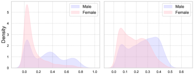
Figure 4: Density of the predicted target variable (salary) across male vs. female, where the idea is that similar distributions should be fairer. Left: w/o our counterfactual mediator regularization. Right: w/ our counterfactual mediator regularization.

5.3 Results for real-world datasets

We now demonstrate the applicability of our method to real-world data. Since ground-truth counterfactuals are unobservable for real-world data, we refrain from benchmarking, but, instead, we now provide additional insights to offer a better understanding of our method.

5.3.1 Results for UCI Adult dataset

Setting: We use UCI Adult (Asuncion & Newman, 2007) to predict if individuals earn a certain salary but where gender is a sensitive attribute. Further details are in Appendix E.

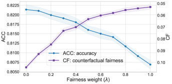
Figure 5: Trade-off between accuracy (ACC) and counterfactual fairness (CF) across different fairness weights $\lambda$. ACC: the higher ($\uparrow$) the better. CF: the lower ($\downarrow$) the better. Shown: mean $\pm$ std over 5 runs.

Insights: To better understand the role of our counterfactual mediator regularization, we trained prediction models both with and without applying $\mathcal{R}_{\mathrm{{cm}}}$. Our primary focus is to show the shifts in the distribution of the predicted target variable (salary) across the sensitive attribute (gender). The corresponding density plots are in Fig. 4. One would expect the distributions for males and females should be more similar if the prediction is fairer. However, we do not see such a tendency for a prediction model without our counterfactual mediator regularization. In contrast, when our counterfactual mediator regularization is used, both distributions are fairly similar as desired. Further visualizations are in Appendix G.

Accuracy and fairness trade-off: We vary the fairness weight $\lambda$ from 0 to 1 to see the trade-off between prediction performance and the level of counterfactual fairness. Since the ground-truth counterfactual is not available for the real-world dataset, we use the generated counterfactual to measure counterfactual fairness on the test dataset. The results are in Fig. 5. In line with our expectations, we see that larger values for $\lambda$ lead the predictions to be more strict w.r.t counterfactual fairness, while lower values allow the predictions to have greater accuracy. Hence, the fairness weight $\lambda$ offers flexibility to decision-makers, so that they can tailor our method to the fairness needs in practice.

5.3.2 Results on COMPAS dataset

Table 2: Comparison of predictions against actual reoffenses.

Method	ACC	PPV	FPR	FNR
COMPAS	0.6644	0.6874	0.4198	0.2689
GCFN (ours)	0.6753	0.7143	0.3519	0.3032
ACC (accuracy); PPV (positive predictive value); FPR (false positive rate); FNR (false negative rate).

Setting: We use the COMPAS dataset (Angwin et al., 2016) to predict recidivism risk of criminals and where race is a sensitive attribute. The dataset also has a COMPAS score for that purpose, yet it was revealed to have racial biases (Angwin et al., 2016). In particular, black defendants were frequently overestimated of their risk of recidivism. Motivated by this finding, we focus our efforts on reducing such racial biases. Further details about the setting are in Appendix E.

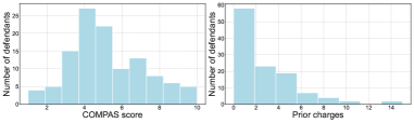
Figure 6: Distribution of black defendants that are treated differently using our GCFN. Left: COMPAS score. Right: Prior charges.

Insights: We first show how our method adds more fairness to real-world applications. For this, we compare the recidivism predictions from the criminal justice process against the actual reoffenses two years later. Specifically, we compute (i) the accuracy of the official COMPAS score in predicting reoffenses and (ii) the accuracy of our GCFN in predicting the outcomes. The results are in Table 2. We see that our GCFN has a better accuracy. More important is the false positive rate (FPR) for black defendants, which measures how often black defendants are assessed at high risk, even though they do not recidivate. Our GCFN reduces the FPR of black defendants from 41.98% to 35.19%. In sum, our method can effectively decrease the bias towards black defendants.

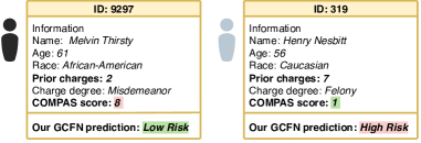
Figure 7: Frequency of how often the predictions from the COMPAS score and our GCFN are different. Shown are the frequency across different COMPAS scores (left) and different numbers of prior charges (right).

We now provide insights at the defendant level to better understand how black defendants are treated differently by the COMPAS score vs. our GCFN. Fig. 6 shows the number of such different treatments across different characteristics of the defendants. (1) Our GCFN makes oftentimes different predictions for black defendants with a medium COMPAS score around 4 and 5. However, the predictions for black defendants with a very high or low COMPAS score are similar, potentially because these are ‘clear-cut’ cases. (2) Our method arrives at significantly different predictions for patients with low prior charges. This is expected as the COMPAS score overestimates the risk and is known to be biased (Angwin et al., 2016). Further insights are in the Appendix G.

To exemplify the above, Fig.7 shows two defendants from the data. Both primarily vary in their race (black vs. white) and their number of prior charges ($2$ vs. $7$). Interestingly, the COMPAS score coincides with race, while our method makes predictions that correspond to the prior charges.

6 Discussion

Flexibility: Our method works with various data types. In particular, it works with both discrete and multi-dimensional sensitive attributes, which are common in practice (De Arteaga et al., 2022). It can also be straightforwardly extended to, e.g., continuous target variables. Our further method offers to choose the fairness-accuracy trade-off according to needs in practice. By choosing a large counterfactual fairness weight $\lambda$, our method enforces counterfactual fairness in a strict manner. Nevertheless, by choosing $\lambda$ appropriately, our method supports applications where practitioners seek a trade-off between performance and fairness.

Limitations. We acknowledge that our method for counterfactual fairness rests on mathematical assumptions, in line with prior work. Further, as with all research on algorithmic fairness, we usher for a cautious, responsible, and ethical use. Sometimes, unfairness may be historically ingrained and require changes beyond the algorithmic layer.

Conclusion: Our work provides a novel method for achieving predictions under counterfactual fairness. Thanks to our combination of the counterfactual mediator regularization with GAN, our GCFN addresses key shortcomings of existing baselines that are based on inferring latent variables, and our GCFN thus achieves state-of-the-art performance.

Appendix A Mathematical background

Notation: Capital letters such as $U$ denote a random variable and small letters $u$ its realizations from corresponding domains $\mathcal{U}$. Bold capital letters such as $\mathbf{U}=\{U_{1},\dots,U_{n}\}$ denote finite sets of random variables. Further, $\mathbb{P}(Y)$ is the distribution of a variable $Y$.

SCM: A structural causal model (SCM) (Pearl, 2009) is a 4-tuple $\langle\mathbf{V},\mathbf{U},\mathcal{F},\mathbb{P}(\mathbf{U})\rangle$, where $\mathbf{U}$ is a set of exogenous (background) variables that are determined by factors outside the model; $\mathbf{V}=\left\{{V}_{1},\ldots,{V}_{n}\right\}$ is a set of endogenous (observed) variables that are determined by variables in the model (i.e., by the variables in $\mathbf{V}\cup\mathbf{U}$ ); $\mathcal{F}=\left\{f_{1},\ldots,f_{n}\right\}$ is the set of structural functions determining $\mathbf{V},v_{i}\leftarrow$ $f_{i}\left(\operatorname{pa}\left(v_{i}\right),u_{i}\right)$, where $\mathrm{pa}\left(V_{i}\right)\subseteq\mathbf{V}\backslash V_{i}$ and $U_{i}\subseteq\mathbf{U}$ are the functional arguments of $f_{i}$; $\mathbb{P}(\mathbf{U})$ is a distribution over the exogenous variables $\mathbf{U}$.

Potential outcome: Let $X$ and $Y$ be two random variables in $\mathbf{V}$ and $\mathbf{u}=\{u_{1},\ldots,u_{n}\}\in\mathcal{U}$ be a realization of exogenous variables. The potential outcome $Y_{x}(\mathbf{u})$ is defined as the solution for $Y$ of the set of equations $\mathcal{F}_{x}$ evaluated with $\mathbf{U}=\mathbf{u}$ (Pearl, 2009). That is, after $\mathbf{U}$ is fixed, the evaluation is deterministic. $Y_{x}(\mathbf{u})$ is the value variable $Y$ would take if (possibly contrary to observed facts) $X$ is set to $x$, for a specific realization $\mathbf{u}$. In the rest of the paper, we use $Y_{x}$ as the short for $Y_{x}(\mathbf{U})$.

Observational distribution: A structural causal model $\mathcal{M}=\langle\mathbf{V},\mathbf{U},\mathcal{F},\mathbb{P}(\mathbf{U})\rangle$ induces a joint probability distribution $\mathbb{P}(\mathbf{V})$ such that for each $Y\subseteq\mathbf{V}$, $\mathbb{P}^{\mathcal{M}}(Y=y)=\sum_{u}\mathds{1}(Y(\mathbf{u})=y)\mathbb{P}(\mathbf{U}=\mathbf{u})$ where $Y(\mathbf{u})$ is the solution for $Y$ after evaluating $\mathcal{F}$ with $\mathbf{U}=\mathbf{u}$ (Bareinboim et al., 2022).

Counterfactual distributions: A structural causal model $\mathcal{M}=\langle\mathbf{V},\mathbf{U},\mathcal{F},\mathbb{P}(\mathbf{U})\rangle$ induces a family of joint distributions over counterfactual events $Y_{x},\ldots,Z_{w}$ for any $Y,Z,\ldots,X,W\subseteq\mathbf{V}$ : $\mathbb{P}^{\mathcal{M}}\left(Y_{x}=y,\ldots,Z_{w}=z\right)=\sum_{u}\mathds{1}\left(Y_{x}(\mathbf{u})=y,\ldots,Z_{w}(\mathbf{u})=z\right)\mathbb{P}(\mathbf{U}=\mathbf{u})$ (Bareinboim et al., 2022). This equation contains variables with different subscripts, which syntactically represent different potential outcomes or counterfactual worlds.

Causal graph: A graph $\mathcal{G}$ is said to be a causal graph of SCM $\mathcal{M}$ if represented as a directed acyclic graph (DAG), where (Pearl, 2009; Bareinboim et al., 2022) each endogenous variable $V_{i}\in\mathbf{V}$ is a node; there is an edge $V_{i}\longrightarrow V_{j}$ if $V_{i}$ appears as an argument of $f_{j}\in\mathcal{F}$ ($V_{i}\in\operatorname{pa}(V_{j})$); there is a bidirected edge $V_{i}\dashleftarrow\dashrightarrow V_{j}$ if the corresponding $U_{i},U_{j}\subset\mathbf{U}$ are correlated ($U_{i}\cap U_{j}\neq\varnothing$) or the corresponding functions $f_{i},f_{j}$ share some $U_{ij}\in\mathbf{U}$ as an argument.

Appendix B Extended Related Work

B.1 Fairness

Recent literature has extensively explored different fairness notions (e.g., Feldman et al., 2015; Di Stefano et al., 2020; Dwork et al., 2012; Grgic.Hlaca et al., 2016; Hardt et al., 2016; Joseph et al., 2016; Pfohl et al., 2019; Salimi et al., 2019; Zafar et al., 2017; Wadsworth et al., 2018; Celis et al., 2019; Chen et al., 2019; Zhang et al., 2018; Madras et al., 2019; Di Stefano et al., 2020; Madras et al., 2018). For a detailed overview, we refer to Makhlouf et al. (2020) and Plecko & Bareinboim (2022). Existing fairness notions can be loosely classified into notions for group- and individual-level fairness, as well as causal notions, some aim at path-specific fairness (e.g., Nabi & Shpitser, 2018; Chiappa, 2019). We adopt the definition of counterfactual fairness from Kusner et al. (2017).

Counterfactual fairness (Kusner et al., 2017): Given a predictive problem with fairness considerations, where $A,X$ and $Y$ represent the sensitive attributes, remaining attributes, and output of interest respectively, for a causal model $\mathcal{M}=\langle\mathbf{V}=\{A,X,Y\},\mathbf{U},\mathcal{F},\mathbb{P}(\mathbf{U})\rangle$, prediction model $\hat{Y}=h(X,A,\mathbf{U})$ is counterfactual fair, if under any context $X=x$ and $A=a$,

$$\mathbb{P}\left(\hat{Y}_{a}(\mathbf{U})\mid X=x,A=a\right)=\mathbb{P}\left(\hat{Y}_{a^{\prime}}(\mathbf{U})\mid X=x,A=a\right),$$ (11)

for any value $a^{\prime}$ attainable by $A$. This is equivalent to the following formulation:

$$\mathbb{P}\left(h(X_{a}(\mathbf{U}),a,\mathbf{U})\mid X=x,A=a\right)=\mathbb{P}\left(h(X_{a^{\prime}}(\mathbf{U}),a^{\prime},\mathbf{U})\mid X=x,A=a\right).$$ (12)

Our paper adapts the later formulation by doing the following. First, we make the prediction model independent of the sensitive attributes $A$, as they could only make the predictive model unfairer. Second, given the general non-identifiability of the posterior distribution of the exogenous noise, i.e., $\mathbb{P}\left(\mathbf{U}\mid X=x,A=a\right)$, we consider only the prediction models dependent on the observed covariates. Third, we split observed covariates $X$ on pre-treatment covariates (confounders) and post-treatment covariates (mediators). Thus, we yield our definition of a fair predictor in Eq. 1.

B.2 Difference from CFGAN

While CFGAN also employs GANs, both the task and the architecture are vastly different from our method.

1. CFGAN uses the GAN to generate entirely synthetic data, while we use the GAN to generate counterfactuals of the mediator. Because of that, our method involves less information loss and leads to better performance at inference.

2. CFGAN has to generate the entire synthetic dataset every time for different downstream tasks, e.g., if the level of fairness requirement changes. In contrast, our method trade-offs accuracy and fairness through our fairness weight $\lambda$ in our regularization, which makes our method more flexible.

3. CFGAN employs a dual-generator and dual-discriminator setup, where each is aimed at simulating the original causal model. Our approach, on the other hand, adopts a streamlined architecture with a singular generator and discriminator. The generator in our model is trained to learn the distribution of the counterfactual mediator, while the discriminator focuses on distinguishing the factual mediator from the generated counterfactual mediator.

4. CFGAN is proposed to synthesize a dataset that satisfies counterfactual fairness. However, a recent paper (Abroshan et al., 2022) has shown that CFGAN is actually considering interventions, not counterfactuals. It does not fulfill this counterfactual fairness notion, but a relevant notion based on do operator (intervention) (see Abroshan et al. (2022), Definition 5 therein, called “Discrimination avoiding through causal reasoning”): A generator is said to be fair if the following equation holds: for any context $A=a$ and $X=x$, for all value of $y$ and $a^{\prime}\in\mathcal{A}$, $P(Y=y\mid X=x,do(A=a))=P\left(Y=y\mid X=x,do\left(A=a^{\prime}\right)\right)$, which is different from the counterfactual fairness $P\left(\hat{Y}_{a}=y\mid X=x,A=a\right)=P\left(\hat{Y}_{a^{\prime}}=y\mid X=x,A=a\right)$. In contrast, our method is theoretically designed to learn a prediction model that can fulfill counterfactual fairness through our novel counterfactual mediator regularization.

Appendix C Training algorithm of GCFN

Algorithm 1 Training algorithm of GCFN

1:Input. Training dataset $\mathcal{D}$; fairness weight $\lambda$; number of training GAN epoch $e_{1}$; number of training prediction model epoch $e_{2}$; minibatch of size $n$; training supervised loss weight $\alpha$

2:Init. Generator ${G}$ parameters: $\theta_{g}$; discriminator ${D}$ parameters: $\theta_{d}$; prediction model $h$ parameters: $\theta_{h}$

3:Step 1: Training GAN to learn to generate counterfactual mediator

4:for $e_{1}$ do

5:     for $k$ steps do $\triangleright$ Training the discriminator $D$

6:         Sample minibatch of $n$ examples $\left\{x^{(i)},a^{(i)},m^{(i)}\right\}_{i=1}^{n}$ from $\mathcal{D}$

7:         Compute generator output ${G}\left({x}^{(i)},{a}^{(i)},{m}^{(i)}\right)_{a}=\hat{m}^{(i)}_{a}\quad\text{for }a\in\{0,1\}$

8:         Modify $G$ output to $\tilde{G}^{(i)}_{a}=\begin{cases}{m}^{(i)},&\text{if }a^{(i)}=a,\\ \hat{m}^{(i)}_{a},&\text{if }a^{(i)}=a^{\prime}\end{cases}\quad\text{for }a\in\{0,1\}$

9:         Update the discriminator via stochastic gradient ascent

$$\nabla_{\theta_{d}}\frac{1}{n}\sum_{i=1}^{n}\left[\log\big{(}{D}({x}^{(i)},\tilde{G}^{(i)})_{a^{(i)}}\big{)}\right]$$

10:     end for

11:     for $k$ steps do $\triangleright$ Training the generator $G$

12:         Sample minibatch of $n$ examples $\left\{x^{(i)},a^{(i)},m^{(i)}\right\}_{i=1}^{n}$ from $\mathcal{D}$

13:         Compute generator output ${G}\left({x}^{(i)},{a}^{(i)},{m}^{(i)}\right)_{a}=\hat{m}^{(i)}_{a}\quad\text{for }a\in\{0,1\}$

14:         Modify $G$ output to $\tilde{G}^{(i)}_{a}=\begin{cases}{m}^{(i)},&\text{if }a^{(i)}=a,\\ \hat{m}^{(i)}_{a},&\text{if }a^{(i)}=a^{\prime}\end{cases}\quad\text{for }a\in\{0,1\}$

15:         Update the generator via stochastic gradient descent

$$\nabla_{\theta_{g}}\frac{1}{n}\sum_{i=1}^{n}\left[\log\big{(}{D}({x}^{(i)},\tilde{G}^{(i)})_{a^{(i)}}\big{)}+\alpha\left\|m^{(i)}-{G}\left({x}^{(i)},{a}^{(i)},{m}^{(i)}\right)_{a^{(i)}}\right\|^{2}_{2}\right]$$

16:     end for

17:end for

18:Step 2: Training prediction model with counterfactual mediator regularization

19:for $e_{2}$ do $\triangleright$ Training the prediction model $h$

20:     Sample minibatch of $n$ examples $\left\{x^{(i)},a^{(i)},m^{(i)},y^{(i)}\right\}_{i=1}^{n}$ from $\mathcal{D}$

21:     Generate $\hat{m}^{(i)}$ from ${G}\left({x}^{(i)},{a}^{(i)},{m}^{(i)}\right)$

22:     Compute counterfactual mediator regularization

$$\mathcal{R}_{\mathrm{{cm}}}=\left\|h(x^{(i)},m^{(i)})-h(x^{(i)},\hat{m}^{(i)}_{a^{{}^{\prime}(i)}})\right\|^{2}_{2}$$

23:     Update the prediction model via stochastic gradient descent

$$\nabla_{\theta_{h}}\frac{1}{n}\sum_{i=1}^{n}\left[y^{(i)}\log\left(h(x^{(i)},m^{(i)})\right)+(1-y^{(i)})\log\left(1-h(x^{(i)},m^{(i)})\right)+\lambda\mathcal{R}_{\mathrm{{cm}}}\right]$$

24:end for

25:Output. Counterfactually fair prediction model $h$

Appendix D Theoretical results

Here, we prove Lemma 1 from the main paper, which states that our counterfactual regularization achieves counterfactual fairness if our generator consistently estimates the counterfactuals.

D.1 Proof of Lemma 1

Lemma 2 (Counterfactual mediator regularization bound).

Given the prediction model $h$ that is Lipschitz continuous with a Lipschitz constant $\mathcal{C}$, we have

$$\mathbb{E}\left[\left\|(h(X,M)-h(X,M_{A^{\prime}})\right\|^{2}_{2}\right]\leq\mathcal{C}\,\mathbb{E}\left[\left\|M_{A^{\prime}}-\hat{M}_{A^{\prime}}\right\|^{2}_{2}\right]+\mathcal{R}_{\mathrm{{cm}}}.$$ (13)

Proof.

Using triangle inequality, we yield

$$\mathbb{E}\left[\left\|h(X,M)-h(X,M_{A^{\prime}})\right\|^{2}_{2}\right]$$ (14)

$$= \,\mathbb{E}\left[\left\|h(X,M)-h(X,M_{A^{\prime}})+h(X,\hat{M}_{A^{\prime}})-h(X,\hat{M}_{A^{\prime}})\right\|^{2}_{2}\right]$$ (15)

$$\leq \,\mathbb{E}\left[\left\|h(X,M)-h(X,\hat{M}_{A^{\prime}})\right\|^{2}_{2}\right]+\mathbb{E}\left[\left\|h(X,\hat{M}_{A^{\prime}})-h(X,M_{A^{\prime}})\right\|^{2}_{2}\right]$$ (16)

$$= \,\mathbb{E}\left[\left\|h(X,\hat{M}_{A^{\prime}})-h(X,M_{A^{\prime}})\right\|^{2}_{2}\right]+\mathcal{R}_{\mathrm{{cm}}}$$ (17)

$$\leq \,\mathcal{C}\,\mathbb{E}\left[\left\|(X,\hat{M}_{A^{\prime}})-({X,{M_{A^{\prime}}}})\right\|^{2}_{2}\right]+\mathcal{R}_{\mathrm{{cm}}}$$ (18)

$$= \,\mathcal{C}\,\mathbb{E}\left[\left\|{M_{A^{\prime}}}-\hat{M}_{A^{\prime}}\right\|^{2}_{2}\right]+\mathcal{R}_{\mathrm{{cm}}}.$$ (19)

∎

D.2 Results on counterfactual consistency

Given Lemma 1, the natural question arises under which conditions our generator produces consistent counterfactuals. In the following, we provide a theory based on bijective generation mechanisms (BGMs) (Nasr-Esfahany et al., 2023; Melnychuk et al., 2023).

Lemma 3 (Consistent estimation of the counterfactual distribution with GAN).

Let the observational distribution $\mathbb{P}_{X,A,M}=\mathbb{P}_{\mathrm{f}}$ be induced by an SCM $\mathcal{M}=\langle\mathbf{V},\mathbf{U},\mathcal{F},\mathbb{P}(\mathbf{U})\rangle$ with

$$\mathbf{V} =\{X,A,M,Y\},\quad\mathbf{U}=\{U_{XA},U_{M},U_{Y}\},$$

$$\mathcal{F} =\{f_{X}(u_{XA}),f_{A}(x,u_{XA}),f_{M}(x,a,u_{M}),f_{Y}(x,m,u_{Y})\},\quad\mathbb{P}(\mathbf{U})=\mathbb{P}(U_{XA})\mathbb{P}(U_{M})\mathbb{P}(U_{Y}),$$

and with the causal graph as in Figure 1. Let $\mathcal{M}\subseteq\mathbb{R}$ and $f_{M}$ be a bijective generation mechanism (BGM) (Nasr-Esfahany et al., 2023; Melnychuk et al., 2023), i.e., $f_{M}$ is a strictly increasing (decreasing) continuously-differentiable transformation wrt. $u_{M}$. Then:

1. The counterfactual distribution of the mediator simplifies to one of two possible point mass distributions

   $$\mathbb{P}(M_{a^{\prime}}\mid X=x,A=a,M=m)=\delta(\mathbb{F}^{-1}(\pm\mathbb{F}(m;x,a)\mp 0.5+0.5;x,a^{\prime})),$$ (20)

   where $\mathbb{F}(\cdot;x,a)$ and $\mathbb{F}^{-1}(\cdot;x,a)$ are a CDF and an inverse CDF of $\mathbb{P}(M\mid X=x,A=a)$, respectively, and $\delta(\cdot)$ is a Dirac-delta distribution;

2. If the generator of GAN is a continuously differentiable function with respect to $M$, then it consistently estimates the counterfactual distribution of the mediator, $\mathbb{P}(M_{a^{\prime}}\mid X=x,A=a,M=m)$, i.e., converges to one of the two solutions in Eq. equation 20.

Proof.

The first statement of the theorem is the main property of bijective generation mechanisms (BGMs), i.e., they allow for deterministic (point mass) counterfactuals. For a more detailed proof, we refer to Lemma B.2 in (Nasr-Esfahany et al., 2023) and to Corollary 3 in (Melnychuk et al., 2023). Importantly, under mild conditions, this result holds in the more general class of BGMs with non-monotonous continuously differentiable functions.

The second statement can be proved in two steps. (i) We show that, given an optimal discriminator, the generator of our GAN estimates the distribution of potential mediators for counterfactual treatments, i.e., $\mathbb{P}(G(x,a,M_{a})_{a^{\prime}}\mid X=x,A=a)=\mathbb{P}(M_{a^{\prime}}\mid X=x,A=a)$ in distribution. (ii) Then, we demonstrate that the outputs of the deterministic generator, conditional on the factual mediator $M=m$, estimate $\mathbb{P}(M_{a^{\prime}}\mid X=x,A=a,M=m)$.

(i) Let $\pi_{a}(x)=\mathbb{P}(A=a\mid X=x)$ denote the propensity score. The discriminator of our GAN, given the covariates $X=x$, tries to distinguish between generated counterfactual data and ground truth factual data. The adversarial objective from Eq. 6 could be expanded with the law of total expectation wrt. $X$ and $A$ in the following way:

$$\mathbb{E}_{({X,A,M)\sim\mathbb{P}_{\mathrm{f}}}}\left[\log\big{(}{D}(X,\tilde{G}\left(X,A,M\right))_{A}\big{)}\right]$$ (21)

$$= \mathbb{E}_{X\sim\mathbb{P}(X)}\mathbb{E}_{({A,M)\sim\mathbb{P}(A,M\mid X)}}\left[\log\big{(}{D}(X,\tilde{G}\left(X,A,M\right))_{A}\big{)}\right]$$ (22)

$$= \mathbb{E}_{X\sim\mathbb{P}(X)}\Big{[}\mathbb{E}_{{M\sim\mathbb{P}(M\mid X,A=0)}}\left[\log\big{(}{D}(X,\tilde{G}\left(X,0,M\right))_{0}\big{)}\right]\,\pi_{0}(X)$$ (23)

$$\qquad\qquad\qquad+\mathbb{E}_{({M\sim\mathbb{P}(M\mid X,A=1)}}\left[\log\big{(}{D}(X,\tilde{G}\left(X,1,M\right))_{1}\big{)}\right]\,\pi_{1}(X)\Big{]}$$

$$= \mathbb{E}_{X\sim\mathbb{P}(X)}\Big{[}\mathbb{E}_{{M\sim\mathbb{P}(M\mid X,A=0)}}\left[\log\big{(}{D}(X,\{M,{G}\left(X,0,M\right)_{1}\})_{0}\big{)}\right]\,\pi_{0}(X)$$ (24)

$$\qquad\qquad\qquad+\mathbb{E}_{{M\sim\mathbb{P}(M\mid X,A=1)}}\left[\log\big{(}1-{D}(X,\{{G}\left(X,1,M\right)_{0},M\})_{0}\big{)}\right]\,\pi_{1}(X)\Big{]}.$$

Let $Z_{0}=\{M,{G}\left(X,0,M\right)_{1}\}$ and $Z_{1}=\{{G}\left(X,1,M\right)_{0},M\}$ be two random variables. Then, using the law of the unconscious statistician, the expression can be converted to a weighted conditional GAN adversarial loss (Mirza & Osindero, 2014), i.e.,

$$\mathbb{E}_{X\sim\mathbb{P}(X)}\Big{[}\mathbb{E}_{{Z_{0}\sim\mathbb{P}(Z_{0}\mid X,A=0)}}\left[\log\big{(}{D}(X,Z_{0})_{0}\big{)}\right]\,\pi_{0}(X)$$ (25)

$$\qquad\qquad\qquad+\mathbb{E}_{{Z_{1}\sim\mathbb{P}(Z_{1}\mid X,A=1)}}\left[\log\big{(}1-{D}(X,Z_{1})_{0}\big{)}\right]\,\pi_{1}(X)\Big{]}$$

$$= \mathbb{E}_{X\sim\mathbb{P}(X)}\bigg{[}\int_{\mathcal{Z}}\Big{(}\log\big{(}{D}(X,z)_{0}\big{)}\,\pi_{0}(X)\mathbb{P}(Z_{0}=z\mid X,A=0)$$ (26)

$$\qquad\qquad\qquad\quad+\log\big{(}1-{D}(X,z)_{0}\big{)}\,\pi_{1}(X)\mathbb{P}(Z_{1}=z\mid X,A=1)\Big{)}\mathop{}\!\mathrm{d}z\bigg{]},$$

where $\mathcal{Z}=\mathcal{M}\times\mathcal{M}$. Notably, the weights of the loss, i.e., $\pi_{0}(X)$ and $\pi_{1}(X)$, are greater than zero, due to the overlap assumption. Following the theory from the standard GANs (Goodfellow et al., 2014b), for any $(a,b)\in\mathbb{R}^{2}\setminus\{0,0\}$, the function $y\mapsto\log(y)a+\log(1-y)b$ achives its maximum in $[0,1]$ at $\frac{a}{a+b}$. Therefore, for a given generator, an optimal discriminator is

$$D(x,z)_{0} =\frac{\mathbb{P}(Z_{0}=z\mid X=x,A=0)\,\pi_{0}(x)}{\mathbb{P}(Z_{0}=z\mid X=x,A=0)\,\pi_{0}(x)+\mathbb{P}(Z_{1}=z\mid X=x,A=1)\,\pi_{1}(x)}.$$ (27)

Both conditional densities used in the expression above can be expressed in terms of the potential outcomes densities due to the consistency and unconfoundedness assumptions, namely

$$\mathbb{P}(Z_{0} =z\mid X=x,A=0)=\mathbb{P}(\{M=m_{0},G(x,0,M)_{1}=m_{1}\}\mid X=x,A=0)$$ (28)

$$=\mathbb{P}(\{M_{0}=m_{0},G(x,0,M_{0})_{1}=m_{1}\}\mid X=x),$$

$$\mathbb{P}(Z_{1} =z\mid X=x,A=1)=\mathbb{P}(\{G(x,1,M)_{0}=m_{0},M=m_{1}\}\mid X=x,A=1)$$ (29)

$$=\mathbb{P}(\{G(x,1,M_{1})_{0}=m_{0},M_{1}=m_{1}\}\mid X=x).$$

Thus, an optimal generator of the GAN then minimizes the following conditional propensity-weighted Jensen–Shannon divergence (JSD)

$$\operatorname{JSD}_{\pi_{0}(x),\pi_{1}(x)} \Big{(}\mathbb{P}(\{M_{0},G(x,0,M_{0})_{1}\}\mid X=x)\,\big{|}\big{|}\,\mathbb{P}(\{G(x,1,M_{1})_{0},M_{1}\}\mid X=x)\Big{)},$$ (30)

where $\operatorname{JSD}_{w_{1},w_{2}}(\mathbb{P}_{1}\,||\,\mathbb{P}_{1})=w_{1}\operatorname{KL}(\mathbb{P}_{1}\,||\,w_{1}\,\mathbb{P}_{1}+w_{2}\,\mathbb{P}_{2})+w_{2}\operatorname{KL}(\mathbb{P}_{2}\,||\,w_{1}\,\mathbb{P}_{1}+w_{2}\,\mathbb{P}_{2})$ and where $\operatorname{KL}(\mathbb{P}_{1}\,||\,\mathbb{P}_{1})$ is Kullback–Leibler divergence. The Jensen–Shannon divergence is minimized, when $G(x,0,M_{0})_{1}=M_{1}$ and $G(x,1,M_{1})_{0}=M_{0}$ conditioned on $X=x$ (in distribution), since, in this case, it equals to zero, i.e.,

$$\mathbb{P}(G(x,a,M_{a})_{a^{\prime}}\mid X=x)=\mathbb{P}(M_{a^{\prime}}\mid X=x).$$ (31)

Finally, due to the unconfoundedness assumption, the generator of our GAN estimates the potential mediator distributions with counterfactual treatments, i.e.,

$$\mathbb{P}(G(x,a,M_{a})_{a^{\prime}}\mid X=x,A=a)=\mathbb{P}(M_{a^{\prime}}\mid X=x,A=a)$$ (32)

in distribution.

(ii) For a given factual observation, $X=x,A=a,M=m$, our generator yields a deterministic output, i.e.,

$$\mathbb{P}(G(x,a,M_{a})_{a^{\prime}}\mid X=x,A=a,M=m) =\mathbb{P}(G(x,a,m)_{a^{\prime}}\mid X=x,A=a,M=m)$$ (33)

$$=\delta(G(x,a,m)_{a^{\prime}}).$$ (34)

At the same time, this counterfactual distribution is connected with the potential mediators’ distributions with counterfactual treatments, $\mathbb{P}(M_{a^{\prime}}=m^{\prime}\mid X=x,A=a)$, via the law of total probability:

$$\mathbb{P}(M_{a^{\prime}}=m^{\prime}\mid X=x,A=a)=\mathbb{P}(G(x,a,M)_{a^{\prime}}=m^{\prime}|X=x,A=a)$$ (35)

$$=\int_{\mathcal{M}}\delta(G(x,a,m)_{a^{\prime}}-m^{\prime})\,\mathbb{P}(M=m\mid X=x,A=a)\mathop{}\!\mathrm{d}m$$ (36)

$$=\sum_{m:\,G(x,a,m)_{a^{\prime}}=m^{\prime}}\,\lvert\,\nabla_{m}G(x,a,m)_{a^{\prime}}\,\rvert^{-1}\,\mathbb{P}(M=m\mid X=x,A=a).$$ (37)

Due to the unconfoundedness and the consistency assumptions, this is equivalent to

$$\mathbb{P}(M=m^{\prime}\mid X=x,A=a^{\prime})=\sum_{m:\,G(x,a,m)_{a^{\prime}}=m^{\prime}}\,\lvert\,\nabla_{m}G(x,a,m)_{a^{\prime}}\,\rvert^{-1}\,\mathbb{P}(M=m\mid X=x,A=a).$$ (38)

The equation above has only two solutions wrt. $G(x,a,\cdot)$ in the class of the continuously differentiable functions (Corollary 3 in (Melnychuk et al., 2023)), namely:

$$G(x,a,m)_{a^{\prime}}=\mathbb{F}^{-1}(\pm\mathbb{F}(m;x,a)\mp 0.5+0.5;x,a^{\prime}),$$ (39)

where $\mathbb{F}(\cdot;x,a)$ and $\mathbb{F}^{-1}(\cdot;x,a)$ are a CDF and an inverse CDF of $\mathbb{P}(M\mid X=x,A=a)$. Thus, the generator of GAN exactly matches one of the two BGM solutions from (i). This concludes that our generator consistently estimates the counterfactual distribution of the mediator, $\mathbb{P}(M_{a^{\prime}}\mid X=x,A=a,M=m)$. ∎

Remark 1.

We proved that the generator converges to one of the two BGM solutions in Eq. 20. Which solution the generator exactly returns depends on the initialization and the optimizer. Notably, the difference between the two solutions is negligibly small, when the entropy of the exogenous variables of the mediator, $\mathbb{P}(U_{M})$, is small. This also holds for high-dimensional mediators, where there is a continuum of solutions in the class of continuously differentiable functions (Chen & Gopinath, 2000). Conversely, if the entropy is high, a combination of multiple GANs might be used to enforce a worst-case counterfactual fairness.

Appendix E Dataset

E.1 Synthetic data

Analogous to prior works that simulate synthetic data for benchmarking (Kim et al., 2021; Kusner et al., 2017; Quinzan et al., 2022), we generate our synthetic dataset in the following way. The covariates $X$ is drawn from a standard normal distribution $\mathcal{N}(0,1)$. The sensitive attribute $A$ follows a Bernoulli distribution with probability $p$, determined by a sigmoid function $\mathrm{\sigma}$ of $X$ and a Gaussian noise term $U_{A}$. We then generate the mediator $M$ as a function of $X$, $A$, and a Gaussian noise term $U_{M}$. Finally, the target $Y$ follows a Bernoulli distribution with probability $p_{y}$, calculated by a sigmoid function of $X$, $M$, and a Gaussian noise term $U_{Y}$. $\beta_{i}\ (i\in[1,6])$ are the coefficients. Let $\sigma(x)=\frac{1}{1+\mathrm{e}^{-x}}$ represent the sigmoid function. Formally, we yield

$$\begin{cases}X=U_{X}&U_{X}\sim\mathcal{N}\left(0,1\right)\\ A\sim\mathrm{Bernoulli}\left(\mathrm{\sigma}(\beta_{1}X+U_{A})\right)&U_{A}\sim\mathcal{N}\left(0,0.01\right)\\ M=\beta_{2}X+\beta_{3}A+U_{M}&U_{M}\sim\mathcal{N}\left(0,0.01\right)\\ Y\sim\mathrm{Bernoulli}\left(\mathrm{\sigma}(\beta_{5}X+\beta_{6}M+U_{Y})\right)&U_{Y}\sim\mathcal{N}\left(0,0.01\right)\\ \end{cases}$$ (40)

We sample 10,000 observations and use 20% as the test set.

E.2 Semi-synthetic data

LSAC dataset. The Law School (LSAC) dataset (Wightman, 1998) contains information about the law school admission records. We use the LSAC dataset to construct two semi-synthetic datasets. In both, we set the sensitive attribute to gender. We take resident and race from the LSAC dataset as confounding variables. The LSAT and GPA are the mediator variables, and the admissions decision is our target variable. We simulate 101,570 samples and use 20% as the test set. We denote $M_{1}$ as GPA score, $M_{2}$ as LSAT score, $X_{1}$ as resident, and $X_{2}$ as race. Further, $w_{X_{1}},w_{X_{2}},w_{A},w_{M_{1}},w_{M_{2}}$ are the coefficients. $U_{M_{1}},U_{M_{2}},U_{Y}$ are the Gaussian noise. Let $\sigma(x)=\frac{1}{1+\mathrm{e}^{-x}}$ represent the sigmoid function.

We then produce the two different semi-synthetic datasets as follows. The main difference is whether we use a rather simple sigmoid function or a complex sinus function that could make extrapolation more challenging for our GCFN.

$\blacksquare$ Semi-synthetic dataset “sigmoid”:

$$\begin{cases}M_{1}=w_{M_{1}}\left(\mathrm{\sigma}(w_{A}A+w_{X_{1}}X_{1}+w_{X_{2}}X_{2}+U_{M_{1}})\right)&U_{M_{1}}\sim\mathcal{N}\left(0,0.01\right)\\ M_{2}=w_{M_{2}}+w_{M_{1}}\left(\mathrm{\sigma}(w_{A}S+w_{X_{1}}X_{1}+w_{X_{2}}X_{2}+U_{M_{2}})\right)&U_{M_{2}}\sim\mathcal{N}\left(0,0.01\right)\\ Y\sim\mathrm{Bernoulli}\left(\mathrm{\sigma}(w_{M_{1}}M_{1}+w_{M_{2}}M_{2}+w_{X_{1}}X_{1}+w_{X_{2}}X_{2}+U_{Y})\right)&U_{Y}\sim\mathcal{N}\left(0,0.01\right)\\ \end{cases}$$ (41)

$\blacksquare$ Semi-synthetic “sin”:

$$\begin{cases}M_{1}=w_{A}\cdot A-\sin\left(\pi\times\left(w_{X_{1}}X_{1}+w_{X_{2}}X_{2}+U_{M_{1}}\right)\right)&U_{M_{1}}\sim\mathcal{N}\left(0,0.01\right)\\ M_{2}=w_{A}\cdot A-\sin\left(\pi\times\left(w_{X_{1}}X_{1}+w_{X_{2}}X_{2}+U_{M_{2}}\right)\right)&U_{M_{2}}\sim\mathcal{N}\left(0,0.01\right)\\ Y\sim\mathrm{Bernoulli}\left(\mathrm{\sigma}(w_{M_{1}}M_{1}+w_{M_{2}}M_{2}+w_{X_{1}}X_{1}+w_{X_{2}}X_{2}+U_{Y})\right)&U_{Y}\sim\mathcal{N}\left(0,0.01\right)\\ \end{cases}$$ (42)

E.3 Real-world data

UCI Adult dataset: The UCI Adult dataset (Asuncion & Newman, 2007) captures information about 48,842 individuals including their sociodemographics. Our aim is to predict if individuals earn more than USD 50k per year. We follow the setting of earlier research (Kim et al., 2021; Nabi & Shpitser, 2018; Quinzan et al., 2022; Xu et al., 2019). We treat gender as the sensitive attribute and set mediator variables to be marital status, education level, occupation, hours per week, and work class. The causal graph of the UCI dataset is in Fig. 8. We take 20% as test set.

COMPAS dataset: COMPAS (Correctional Offender Management Profiling for Alternative Sanctions) (Angwin et al., 2016) was developed as a decision support tool to score the likelihood of a person’s recidivism. The score ranges from 1 (lowest risk) to 10 (highest risk). The dataset further contains information about whether there was an actual recidivism (reoffended) record within 2 years after the decision. Overall, the dataset has information about over 10,000 criminal defendants in Broward County, Florida. We treat race as the sensitive attribute. The mediator variables are the features related to prior convictions and current charge degree. The target variable is the recidivism for each defendant. The causal graph of the COMPAS dataset is in Fig. 9. We take 20% as test set.

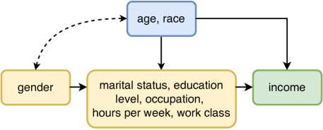
Figure 8: Causal graph of UCI dataset.

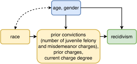
Figure 9: Causal graph of COMPAS dataset.

Appendix F Implementation Details

F.1 Implementation of benchmarks

We implement CFAN (Kusner et al., 2017) in PyTorch based on the paper’s source code in R and Stan on https://github.com/mkusner/counterfactual-fairness. We use a VAE to infer the latent variables. For mCEVAE (Pfohl et al., 2019), we follow the implementation from https://github.com/HyemiK1m/DCEVAE/tree/master/Tabular/mCEVAE_baseline. We implement CFGAN (Xu et al., 2019) in PyTorch based on the code of Abroshan et al. (2022) and the TensorFlow source code of (Xu et al., 2019). We implement ADVAE (Grari et al., 2023) in PyTorch. For DCEVAE (Kim et al., 2021), we use the source code of the author of DCEVAE (Kim et al., 2021). We use HSCIC (Quinzan et al., 2022) source implementation from the supplementary material provided on the OpenReview website https://openreview.net/forum?id=ERjQnrmLKH4. We performed rigorous hyperparameter tuning for all baselines.

Hyperparameter tuning. We perform a rigorous procedure to optimize the hyperparameters for the different methods as follows. For DCEVAE (Kim et al., 2021) and mCEVAE (Pfohl et al., 2019), we follow the hyperparameter optimization as described in the supplement of Kim et al. (2021). For ADVAE (Grari et al., 2023) and CFGAN (Xu et al., 2019), we follow the hyperparameter optimization as described in their paper. For both HSCIC and our GCFN, we have an additional weight that introduces a trade-off between accuracy and fairness. This provides additional flexibility to decision-makers as they tailor the methods based on the fairness needs in practice Quinzan et al. (2022). We then benchmark the utility of different methods across different choices of $\gamma$ of the utility function in Sec. 5.1. This allows us thus to optimize the trade-off weight $\lambda$ inside HSCIC and our GCFN using grid search. For HSCIC, we experiment with $\lambda=0.1,0.5,1,5,10,15,20$ and choose the best for them across different datasets. For our method, we experiment with $\lambda=0.1,0.5,1,1.5,2$. Since the utility function considers two metrics, across the experiments on (semi-)synthetic dataset, the weight $\lambda$ is set to $0.5$ to get a good balance for our method.

F.2 Implementation of our method

Our GCFN is implemented in PyTorch. Both the generator and the discriminator in the GAN model are designed as deep neural networks, each with a hidden layer of dimension $64$. LeakyReLU is employed as the activation function and batch normalization is applied in the generator to enhance training stability. The GAN training procedure is performed for $300$ epochs with a batch size of $256$ at each iteration. We set the learning rate to $0.0005$. Following the GAN training, the prediction model, structured as a multilayer perceptron (MLP), is trained separately. This classifier can incorporate spectral normalization in its linear layers to ensure Lipschitz continuously. It is trained for $30$ epochs, with the same learning rate of $0.005$ applied. The training time of our GCFN on (semi-) synthetic dataset is comparable to or smaller than the baselines.

Appendix G Additional experimental results

G.1 Results for (semi-)synthetic dataset

We compute the average value of the utility function $U$ over varying utility weights $\gamma\in\{0.1,\ldots,1.0\}$ on the synthetic dataset (Fig. 10) and two different semi-synthetic datasets (Fig. 11 and Fig. 12).

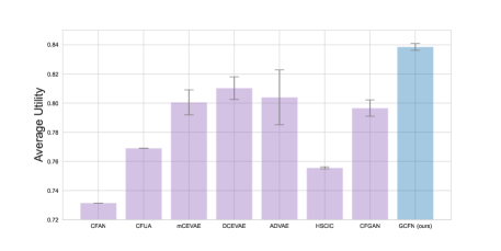
Figure 10: Average utility function value $U$ across different utility weights $\gamma$ on synthetic dataset.

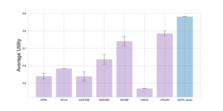
Figure 11: Average utility function value $U$ across different utility weight $\gamma$ on semi-synthetic (sigmoid) dataset.

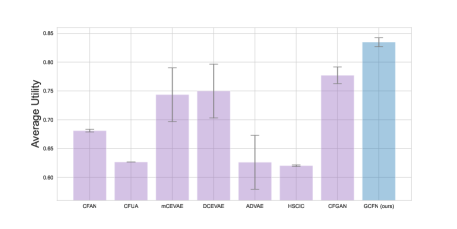
Figure 12: Average utility function value $U$ across different utility weight $\gamma$ on semi-synthetic (sin) dataset.

G.2 Results for UCI Adult dataset

We now examine the results for different fairness weights $\lambda$. For this, we report results from $\lambda=0.5$ (Fig. 13) to $\lambda=1000$ (Fig. 16). In line with our expectations, we see that larger values for fairness weight $\lambda$ lead the distributions of the predicted target to overlap more, implying that counterfactual fairness is enforced more strictly. This shows that our regularization $\mathcal{R}_{\mathrm{{cm}}}$ achieves the desired behavior.

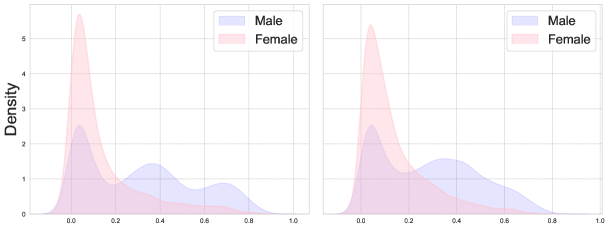
Figure 13: Density plots of the predicted target on UCI Adult dataset. Left: fairness weight $\lambda=0$. Right: fairness weight $\lambda=0.5$.

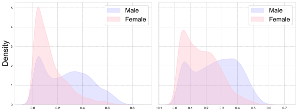
Figure 14: Density plots of the predicted target on UCI Adult dataset. Left: fairness weight $\lambda=1$. Right: fairness weight $\lambda=5$.

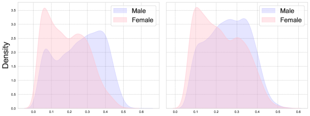
Figure 15: Density plots of the predicted target on UCI Adult dataset. Left: fairness weight $\lambda=10$. Right: fairness weight $\lambda=100$.

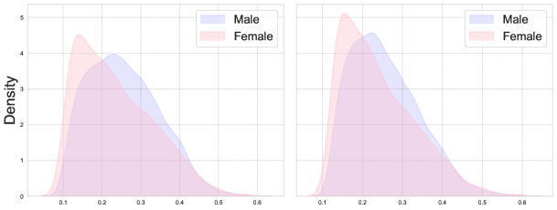
Figure 16: Density plots of the predicted target on UCI Adult dataset. Left: fairness weight $\lambda=500$. Right: fairness weight $\lambda=1000$.

G.3 Results for COMPAS dataset

In Sec. 5, we show how black defendants are treated differently by the COMPAS score vs. our GCFN. Here, we also show how white defendants are treated differently by the COMPAS score vs. our GCFN; see Fig. 17. We make the following observations. (1) Our GCFN makes oftentimes different predictions for white defendants with a low and high COMPAS score, which is different from black defendants. (2) Our method also arrives at different predictions for white defendants with low prior charges, similar to black defendants.

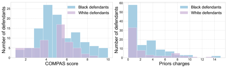
Figure 17: Distribution of white and black defendants that are treated differently using our GCFN. Left: COMPAS score. Right: Prior charges.

References

- Abroshan et al. (2022) Mahed Abroshan, Mohammad Mahdi Khalili, and Andrew Elliott. Counterfactual fairness in synthetic data generation. In NeurIPS 2022 Workshop on Synthetic Data for Empowering ML Research, 2022.
- Angwin et al. (2016) Julia Angwin, Jeff Larson, Surya Mattu, and Lauren Kirchner. Machine bias: There’s software used across the country to predict future criminals and it’s biased against blacks. In ProPublica, 2016.
- Asuncion & Newman (2007) Arthur Asuncion and David Newman. UCI machine learning repository, 2007.
- Bareinboim et al. (2022) Elias Bareinboim, Juan D Correa, Duligur Ibeling, and Thomas Icard. On Pearl’s hierarchy and the foundations of causal inference. In Probabilistic and causal inference: the works of Judea Pearl, 2022.
- Barocas & Selbst (2016) Solon Barocas and Andrew D. Selbst. Big data’s disparate impact. California Law Review, 2016.
- Bica et al. (2020) Ioana Bica, James Jordon, and Mihaela van der Schaar. Estimating the effects of continuous-valued interventions using generative adversarial networks. In NeurIPS, 2020.
- Celis et al. (2019) L Elisa Celis, Lingxiao Huang, Vijay Keswani, and Nisheeth K Vishnoi. Classification with fairness constraints: A meta-algorithm with provable guarantees. In FAacT, 2019.
- Chen et al. (2019) Jiahao Chen, Nathan Kallus, Xiaojie Mao, Geoffry Svacha, and Madeleine Udell. Fairness under unawareness: Assessing disparity when protected class is unobserved. In FAacT, 2019.
- Chen & Gopinath (2000) Scott Chen and Ramesh Gopinath. Gaussianization. In NeurIPS, 2000.
- Chiappa (2019) Silvia Chiappa. Path-specific counterfactual fairness. In AAAI, 2019.
- De Arteaga et al. (2022) Maria De Arteaga, Stefan Feuerriegel, and Maytal Saar.Tsechansky. Algorithmic fairness in business analytics: Directions for research and practice. Production and Operations Management, 2022.
- Di Stefano et al. (2020) Pietro G Di Stefano, James M Hickey, and Vlasios Vasileiou. Counterfactual fairness: removing direct effects through regularization. In arXiv preprint, 2020.
- Dwork et al. (2012) Cynthia Dwork, Moritz Hardt, Toniann Pitassi, Omer Reingold, and Richard Zemel. Fairness through awareness. In Innovations in Theoretical Computer Science Conference, 2012.
- Feldman et al. (2015) Michael Feldman, Sorelle A Friedler, John Moeller, Carlos Scheidegger, and Suresh Venkatasubramanian. Certifying and removing disparate impact. In KDD, 2015.
- Feuerriegel et al. (2020) Stefan Feuerriegel, Mateusz Dolata, and Gerhard Schwabe. Fair ai: Challenges and opportunities. Business & Information Systems Engineering, 62:379–384, 2020.
- Garg et al. (2019) Sahaj Garg, Vincent Perot, Nicole Limtiaco, Ankur Taly, Ed H Chi, and Alex Beutel. Counterfactual fairness in text classification through robustness. In AIES, 2019.
- Goodfellow et al. (2014a) Ian Goodfellow, Jean Pouget.Abadie, Mehdi Mirza, Bing Xu, David Warde.Farley, Sherjil Ozair, Aaron Courville, and Yoshua Bengio. Generative adversarial nets. In NeurIPS, 2014a.
- Goodfellow et al. (2014b) Ian J. Goodfellow, Jean Pouget.Abadie, Mehdi Mirza, Bing Xu, David Warde.Farley, Sherjil Ozair, Aaron Courville, and Yoshua Bengio. Generative Adversarial Networks (GAN), June 2014b.
- Grari et al. (2023) Vincent Grari, Sylvain Lamprier, and Marcin Detyniecki. Adversarial learning for counterfactual fairness. Machine Learning, 2023.
- Grgic.Hlaca et al. (2016) Nina Grgic.Hlaca, Muhammad Bilal Zafar, Krishna P Gummadi, and Adrian Weller. The case for process fairness in learning: Feature selection for fair decision making. In NIPS Symposium on Machine Learning and the Law, 2016.
- Hardt et al. (2016) Moritz Hardt, Eric Price, and Nati Srebro. Equality of opportunity in supervised learning. In NeurIPS, 2016.
- Joseph et al. (2016) Matthew Joseph, Michael Kearns, Jamie Morgenstern, Seth Neel, and Aaron Roth. Fair algorithms for infinite and contextual bandits. arXiv preprint, 2016.
- Kim et al. (2021) Hyemi Kim, Seungjae Shin, JoonHo Jang, Kyungwoo Song, Weonyoung Joo, Wanmo Kang, and Il.Chul Moon. Counterfactual fairness with disentangled causal effect variational autoencoder. In AAAI, 2021.
- Kleinberg et al. (2019) Jon Kleinberg, Jens Ludwig, Sendhil Mullainathan, and Cass R. Sunstein. Discrimination in the age of algorithms. Journal of Legal Analysis, 2019.
- Kocaoglu et al. (2018) Murat Kocaoglu, Christopher Snyder, Alexandros G Dimakis, and Sriram Vishwanath. CausalGAN: Learning causal implicit generative models with adversarial training. In ICLR, 2018.
- Kusner et al. (2017) Matt J Kusner, Joshua Loftus, Chris Russell, and Ricardo Silva. Counterfactual fairness. In NeurIPS, 2017.
- Louizos et al. (2017) Christos Louizos, Uri Shalit, Joris M Mooij, David Sontag, Richard Zemel, and Max Welling. Causal effect inference with deep latent-variable models. In NeurIPS, 2017.
- Ma et al. (2023) Jing Ma, Ruocheng Guo, Aidong Zhang, and Jundong Li. Learning for counterfactual fairness from observational data. In KDD, 2023.
- Madras et al. (2018) David Madras, Elliot Creager, Toniann Pitassi, and Richard Zemel. Learning adversarially fair and transferable representations. In ICML, 2018.
- Madras et al. (2019) David Madras, Elliot Creager, Toniann Pitassi, and Richard Zemel. Fairness through causal awareness: Learning causal latent-variable models for biased data. In FAacT, 2019.
- Makhlouf et al. (2020) Karima Makhlouf, Sami Zhioua, and Catuscia Palamidessi. Survey on causal-based machine learning fairness notions. arXiv preprint, 2020.
- Melnychuk et al. (2023) Valentyn Melnychuk, Dennis Frauen, and Stefan Feuerriegel. Partial counterfactual identification of continuous outcomes with a curvature sensitivity model. In NeurIPS, 2023.
- Mirza & Osindero (2014) Mehdi Mirza and Simon Osindero. Conditional generative adversarial nets. arXiv preprint arXiv:1411.1784, 2014.
- Nabi & Shpitser (2018) Razieh Nabi and Ilya Shpitser. Fair inference on outcomes. In AAAI, 2018.
- Nasr-Esfahany et al. (2023) Arash Nasr-Esfahany, Mohammad Alizadeh, and Devavrat Shah. Counterfactual identifiability of bijective causal models. In ICML, 2023.
- Pawlowski et al. (2020) Nick Pawlowski, Daniel Coelho de Castro, and Ben Glocker. Deep structural causal models for tractable counterfactual inference. In NeurIPS, 2020.
- Pearl (2009) Judea Pearl. Causal inference in statistics: An overview. Statistics Surveys, 2009.
- Pfohl et al. (2019) Stephen R. Pfohl, Tony Duan, Daisy Yi Ding, and Nigam H Shah. Counterfactual reasoning for fair clinical risk prediction. In Machine Learning for Healthcare Conference, 2019.
- Plecko & Bareinboim (2022) Drago Plecko and Elias Bareinboim. Causal fairness analysis. In arXiv preprint, 2022.
- Quinzan et al. (2022) Francesco Quinzan, Cecilia Casolo, Krikamol Muandet, Niki Kilbertus, and Yucen Luo. Learning counterfactually invariant predictors. arXiv preprint, 2022.
- Rajabi & Garibay (2022) Amirarsalan Rajabi and Ozlem Ozmen Garibay. Tabfairgan: Fair tabular data generation with generative adversarial networks. In Machine Learning and Knowledge Extraction, 2022.
- Rubin (1974) Donald B. Rubin. Estimating causal effects of treatments in randomized and nonrandomized studies. Journal of Educational Psychology, 66(5):688–701, 1974. ISSN 0022-0663. doi: 10.1037/h0037350.
- Salimi et al. (2019) Babak Salimi, Luke Rodriguez, Bill Howe, and Dan Suciu. Interventional fairness: Causal database repair for algorithmic fairness. In International Conference on Management of Data, 2019.
- van Breugel et al. (2021) Boris van Breugel, Trent Kyono, Jeroen Berrevoets, and Mihaela van der Schaar. DECAF: Generating fair synthetic data using causally-aware generative networks. In NeurIPS, 2021.
- von Zahn et al. (2022) Moritz von Zahn, Stefan Feuerriegel, and Niklas Kuehl. The cost of fairness in ai: Evidence from e-commerce. Business & Information Systems Engineering, 64:335–348, 2022.
- Wadsworth et al. (2018) Christina Wadsworth, Francesca Vera, and Chris Piech. Achieving fairness through adversarial learning: an application to recidivism prediction. In arXiv preprint, 2018.
- Wightman (1998) Linda F Wightman. LSAC National Longitudinal Bar Passage Study. LSAC Research Report Series. In ERIC, 1998.
- Xu et al. (2018) Depeng Xu, Shuhan Yuan, Lu Zhang, and Xintao Wu. FairGAN: Fairness-aware generative adversarial networks. In ICBD, 2018.
- Xu et al. (2019) Depeng Xu, Yongkai Wu, Shuhan Yuan, Lu Zhang, and Xintao Wu. Achieving causal fairness through generative adversarial networks. In IJCAI, 2019.
- Yoon et al. (2018) Jinsung Yoon, James Jordon, and Mihaela van der Schaar. GANITE: Estimation of individualized treatment effects using generative adversarial nets. In ICLR, 2018.
- Zafar et al. (2017) Muhammad Bilal Zafar, Isabel Valera, Manuel Gomez Rogriguez, and Krishna P Gummadi. Fairness constraints: Mechanisms for fair classification. In AISTATS, 2017.
- Zhang et al. (2018) Brian Hu Zhang, Blake Lemoine, and Margaret Mitchell. Mitigating unwanted biases with adversarial learning. In AIES, 2018.