Validation of Spherical Fourier-Bessel power spectrum analysis with lognormal simulations and eBOSS DR16 LRG EZmocks

Abstract

Tuning into the bass notes of the large-scale structure requires careful attention to geometrical effects arising from wide angles. The spherical Fourier-Bessel (SFB) basis provides a harmonic-space coordinate system that fully accounts for all wide-angle effects. To demonstrate the feasibility of the SFB power spectrum, in this paper we validate our SFB pipeline by applying it to lognormal, and both complete and realistic EZmock simulations that were generated for eBOSS DR16 LRG sample. We include redshift space distortions and the local average effect (aka integral constraint). The covariance matrix is obtained from 1000 EZmock simulations, and inverted using eigenvalue decomposition.

I Introduction

Upcoming galaxy surveys such as SPHEREx, Euclid, DESI, PFS, and others will have significant constraining power on very large scales. This will allow constraints on local-type primordial non-Gaussianity that is predicted by inflation.

The typical power spectrum multipole estimator was introduced by Yamamoto et al. (2006) (for a review and implementation see Hand et al., 2017, e.g.). In the Yamamoto estimator, a single line-of-sight (LOS) is chosen for each pair of galaxies, and for efficient implementation that LOS is typically chosen to one of the galaxies in each pair. However, while the Yamamoto estimator is a significant improvement over the assumption of a flat sky with a fixed LOS, it still suffers from wide-angle effects that can mimic a non-Gaussianity parameter $f_{\mathrm{NL}}\sim 5$ (Benabou et al., prep). Further extensions to the Yamamoto estimator such as using the midpoint or bisector between the galaxy pair as the LOS (Philcox and Slepian, 2021) are also possible. However, while certainly less, those estimators, too, will contain wide-angle effects.

The spherical Fourier-Bessel decomposition fully accounts for all wide-angle effects, because it is the natural coordinate system for the radial/angular separation. (Heavens and Taylor, 1995; Percival et al., 2004; Wang et al., 2020; Grasshorn Gebhardt and Doré, 2021)

In this paper we validate the SFB power spectrum estimator developed in Grasshorn Gebhardt and Doré (2021) on the realistic eBOSS DR16 luminous red galaxy EZmocks (Zhao et al., 2021). For the covariance matrix we use all 1000 EZmocks.

This paper is organized as follows. In Section II we review the SFB basis, in Section III we review our SuperFaB estimator, in Section IV we detail the theoretical modeling including window, weights, shot noise, local average effect, and pixel window. We validate our analysis pipeline with lognormal mocks in Section V, and with EZmocks in Section VI. The likelihood is constructed and run with an adaptive Metropolis-Hastings sampler in Section VII. We conclude in Section VIII. Many details such as a derivation of the local average effect and velocity boundary conditions are delegated to the appendices.

II Spherical Fourier-Bessel basis

Similar to the Cartesian basis power spectrum analysis, the spherical Fourier-Bessel analysis also separates scales according to a wavenumber $k$. This stems from the Laplacian eigenequation $\nabla^{2}f=-k^{2}f$ that defines both bases, with the difference coming mainly from the geometry of the boundary conditions.

The spherical Fourier-Bessel basis offers several advantages and disadvantages over the more familiar Cartesian-space analysis. The two chief advantages of SFB is in the separation of angular and radial modes due to the use of spherical polar coordinates, and in the complete modeling of wide-angle effects. Many observational effects are local in origin, and, thus, manifest themselves purely as angular systematics. Wide-angle effects come from the geometry of the curved sky, and they have a similar signature as local non-Gaussianity in the endpoint estimator (Yamamoto et al., 2006; Bianchi et al., 2015; Scoccimarro, 2015; Hand et al., 2017; Castorina and White, 2020; Beutler et al., 2019). Due to the use of a spherical coordinate system and spherical boundaries, SFB is well-suited for both these types of systematics.

Besides the lesser familiarity of the SFB power spectrum compared to Cartesian-space power spectrum multipoles, the SFB power spectrum suffers from an increased computational cost due to the lack of the fast Fourier-transform, and it suffers from an increase in the number of modes. The large number of modes contains a wealth of information that may be exploited, such as distinguishing between redshift space distortions and evolution of galaxy bias and growth rate with redshift, to name a few. However, the presence of so many modes also presents challenges in the analysis.

The spherical Fourier-Bessel basis is defined by the eigenfunctions of the Laplacian in spherical polar coordinates with spherical boundaries. Thus, the density contrast is expanded in SFB coefficients as (e.g. Nicola et al., 2014)

$$\delta({\bm{r}}) =\sum_{n\ell m}g_{n\ell}(r)\,Y_{\ell m}({\hat{\bm{r}}})\,\delta_{n\ell m}\,,$$ (1)

$$\delta_{n\ell m} =\int\mathrm{d}^{3}{\bm{r}}\,g_{n\ell}(r)\,Y^{*}_{\ell m}({\hat{\bm{r}}})\,\delta({\bm{r}})\,,$$ (2)

where the second is the inverse of the first, and $Y_{\ell m}({\hat{\bm{r}}})$ are spherical harmonics, and

$$g_{n\ell}(r)=c_{n\ell}\,j_{\ell}(k_{n\ell}r)+d_{n\ell}\,y_{\ell}(k_{n\ell}r)$$ (3)

are linear combinations of spherical Bessel functions of the first and second kind, chosen to satisfy the orthonormality relation

$$\int_{r_{\mathrm{min}}}^{r_{\mathrm{max}}}\mathrm{d}r\,r^{2}\,g_{n\ell}(r)\,g_{n^{\prime}\ell}(r) =\delta^{K}_{nn^{\prime}}\,.$$ (4)

The index $n$ denotes the wavenumber $k_{n\ell}$, and $c_{n\ell}$ and $d_{n\ell}$ are constants (Samushia, 2019; Grasshorn Gebhardt and Doré, 2021). For comparison, we include the SFB transform over an infinite flat universe in Eqs. 35 and 36.

In this paper, we assume potential boundaries (Fisher et al., 1995) which ensure that the density contrast is continuous and smooth on the boundaries. Further, we assume a spherical boundary at some minimum distance $r_{\mathrm{min}}$ and some maximum distance $r_{\mathrm{max}}$ so that the SFB analysis is performed in a thick shell between $r_{\mathrm{min}}$ and $r_{\mathrm{max}}$ (Grasshorn Gebhardt and Doré, 2021; Samushia, 2019). We have also verified that velocity boundary conditions (that ensure vanishing derivative at the boundary) give essentially the same result, see Section V.2.3.

III SuperFaB estimator

For our SFB estimator we use SuperFaB. We refer the interested reader to Grasshorn Gebhardt and Doré (2021) for all the details, and give only a very short overview here. In brief, SuperFaB is similar to the 3DEX approach developed in Leistedt et al. (2012). SuperFaB assumes the number density is given by a discrete set of points,

$$n({\bm{r}}) =\sum_{p}\delta^{D}({\bm{r}}-{\bm{r}}_{p})\,,$$ (5)

where the sum is over all points (galaxies) in the survey. To calculate the fluctuation field, we include a weighting (Feldman et al., 1994)

$$w({\bm{r}}) =\frac{1}{1+{\bar{n}}\,W({\bm{r}})\,C_{\ell nn^{\prime}}}\,,$$ (6)

and we approximate $C_{\ell nn^{\prime}}\sim${10}^{4}\text{\,}{\mathrm{\text{$h$}}}^{-3}\text{\,}{\mathrm{Mpc}}^{3}$$, so that the observed density fluctuation field is

$$\delta^{\mathrm{obs}}({\bm{r}}) =w({\bm{r}})\,\frac{n({\bm{r}})-\alpha\,n_{r}({\bm{r}})}{{\bar{n}}_{\mathrm{max}}}\,,$$ (7)

where $n({\bm{r}})$ is the observed number density and $n_{r}({\bm{r}})$ is a uniform random catalog subject to the same window function and systematics. ${\bar{n}}_{\mathrm{max}}$ is the maximum number density in the data catalog, in our convention.

To perform the discrete SFB transform Eq. 2, we first perform the radial integral for each $(n,\ell)$ combination by directly summing over the galaxies, and pixelizing on the spherical sky using the HEALPix scheme (Górski et al., 2005). The angular integration is then performed using HEALPix.jl (Tomasi and Li, 2021).

This SFB transform is performed for both the data catalog and the random catalog, and the result is subtracted with appropriate normalization to obtain the fluctuation field $\hat{\delta}_{n\ell m}$.

Finally, we construct the pseudo-SFB power spectrum

$$\hat{C}^{wWA}_{\ell nn^{\prime}} =\frac{1}{2\ell+1}\sum_{m}\hat{\delta}_{n\ell m}\hat{\delta}^{*}_{n^{\prime}\ell m}\,,$$ (8)

where we attach the suffixes ‘$wW$’ for the weight and window, and the suffix ‘$A$’ for the local average effect, and the caret ($\hat{\phantom{x}}$) indicates estimation from data. Window function and other effects will be forward-modeled, and we turn to that next.

IV SFB Power Spectrum Model

In this section we detail our approach for calculating a theoretical model for the estimator of Section III. We start with a full-sky calculation, and then add the window function, weights, local average effect (LAE), and pixel window. In the window function we generally include survey geometry and radial selection function.

In the SFB basis, the full-sky linear power spectrum $C_{\ell nn^{\prime}}\simeq C_{\ell}(k_{n\ell},k_{n^{\prime}\ell})$ on the lightcone in redshift space is expressed as (Khek et al., 2022)

$$C_{\ell nn^{\prime}} =\int_{0}^{\infty}\mathrm{d}q\,\mathcal{W}_{n\ell}(q)\,\mathcal{W}_{n^{\prime}\ell}(q)\,\gamma^{-3}\,P_{m}(\gamma^{-1}q)\,,$$ (9)

where $P_{m}(q)$ is the matter power spectrum, $\gamma$ is an Alcock-Paczynski-like parameter, and

$$\mathcal{W}_{n\ell}(q) =\sqrt{\frac{2}{\pi}}\,q\int_{r_{\mathrm{min}}}^{r_{\mathrm{max}}}\mathrm{d}r\,r^{2}\,g_{n\ell}(r)\,w(r)\,\phi(r)\,D(r)$$

$$\quad\times e^{\frac{1}{2}\sigma_{u}^{2}q^{2}\partial_{qr}^{2}}\left[b(r,q)\,j_{\ell}(qr)-f(r)\,j^{\prime\prime}_{\ell}(qr)\right],$$ (10)

with the radial basis functions $g_{n\ell}(r)$ defined in Eq. 3, where $w(r)$ is a weighting function, $\phi(r)$ is a radial selection function, $D(r)$ is the linear growth factor, $b(r,q)$ is a scale-dependent linear galaxy bias, $\sigma_{u}^{2}$ is a velocity dispersion, and $f$ is the linear growth rate.

The velocity dispersion term we approximate by expanding the exponential operator (that acts on the spherical Bessels only) in a Taylor series to get

$$e^{\frac{1}{2}\sigma_{u}^{2}q^{2}\partial_{qr}^{2}}j^{(d)}_{\ell}(qr) \approx j^{(d)}_{\ell}(qr)-\frac{1}{2}\sigma_{u}^{2}q^{2}\,j^{(d+2)}_{\ell}(qr)\,,$$ (11)

where $j_{\ell}^{(d)}(qr)$ is the $d$th derivative w.r.t. $qr$.

The velocity dispersion is a combination of Fingers-of-God (FoG) effect and redshift measurement uncertainty, $\sigma_{u}^{2}=\sigma_{u,\mathrm{FoG}}^{2}+\sigma_{z}^{2}$. The FoG effect is modeled to be proportional to the linear growth rate $f(z)$. The redshift measurement uncertainty is kept constant $1.05\text{\,}{\mathrm{\text{$h$}}}^{-1}\text{\,}\mathrm{Mpc}$ in our model, taken from Ross et al. (2020, their Fig. 2).

Local non-Gaussianity is modeled via a scale-dependent bias (Dalal et al., 2008)

$$b(r,q) =b(r)+f_{\mathrm{NL}}b_{\phi}(r)\,\frac{3\Omega_{m}H_{0}^{2}}{2q^{2}T(q)\bar{D}(r)}\,,$$ (13)

where for this paper we assume the universal bias relation (Dalal et al., 2008; Slosar et al., 2008; Afshordi and Tolley, 2008; Matarrese and Verde, 2008)

$$b_{\phi}(r) =2\delta_{c}\,[b(r)-1]\,,$$ (14)

$T(q)$ is the transfer function, and $\bar{D}(r)$ is the growth factor normalized to the scale factor $a$ during matter domination,

$$\bar{D}(r) =\frac{D(r)}{(1+z_{\mathrm{md}})\,D(r_{\mathrm{md}})}\,,$$ (15)

where the “$\mathrm{md}$” suffix indicates a time deep within matter domination.

In its most complete form, the SFB power spectrum contains off-diagonal terms where $k_{n\ell}\neq k_{n^{\prime}\ell}$. In a homogeneous universe we would have $C_{\ell}(k,k^{\prime})\,\propto\,\delta^{D}(k-k^{\prime})$. However, both redshift space distortions and growth of structure on the light cone break homogeneity in the observed galaxy sample. For details we refer the reader to Pratten and Munshi (2013, 2014); Khek et al. (2022).

The bulk of the computation is spent on the spherical Bessel functions in $\mathcal{W}_{n\ell}(q)$ in Section IV. However, those only depend on the combination $qr$, not on $q$ and $r$ separately. Thus, we choose discretizations for $q$ and $r$ such that in $q$-$r$ space the “iso-$qr$” lines go precisely through grid points. This condition demands that the discretizations for $q$ and $r$ are logarithmic, i.e.,

$$q_{i} =\bar{q}_{\mathrm{min}}\,R^{i\Delta n}\,,$$ (16)

$$r_{j} =\bar{r}_{\mathrm{min}}\,R^{j}\,,$$ (17)

where $\bar{q}_{\mathrm{min}}$ and $\bar{r}_{\mathrm{min}}$ are the central values of the lowest bins, $\ln R$ is the spacing in log-space, and $\Delta n\geq 1$ is an integer to allow sparse sampling of $q$. Then, $qr$ is sampled at only a few discrete $m=i\Delta n+j$,

$$(qr)_{m} =\bar{q}_{\mathrm{min}}\bar{r}_{\mathrm{min}}\,R^{i\Delta n+j}\,.$$ (18)

This transforms the problem of calculating the spherical Bessels from a 2-dimensional to a 1-dimensional problem.

IV.1 Window function convolution

The window function limits the density contrast to that observed by a survey $\delta^{\mathrm{obs}}({\bm{r}})=W({\bm{r}})\,\delta({\bm{r}})$, where we define the window $W({\bm{r}})=\bar{n}({\bm{r}})/{\bar{n}}_{\mathrm{max}}$. In SFB space the window effect becomes a convolution,

$$\delta^{\mathrm{obs}}_{n\ell m} =\sum_{NLM}W_{n\ell m}^{NLM}\,\delta_{NLM}\,,$$ (19)

where the coupling matrix is

$$W_{n\ell m}^{n^{\prime}\ell^{\prime}m^{\prime}} =\int\mathrm{d}r\,r^{2}\,g_{n\ell}(r)\,g_{n^{\prime}\ell^{\prime}}(r)$$

$$\quad\times\int\mathrm{d}^{2}{\hat{\bm{r}}}\,Y^{*}_{\ell m}({\hat{\bm{r}}})\,Y_{\ell^{\prime}m^{\prime}}({\hat{\bm{r}}})\,W(r,{\hat{\bm{r}}})\,.$$ (20)

As a result, the modes of the SFB power spectrum are coupled,

$$C^{\mathrm{obs}}_{\ell nn^{\prime}}=\sum_{LNN^{\prime}}\mathcal{M}_{\ell nn^{\prime}}^{LNN^{\prime}}\,C_{LNN^{\prime}}\,,$$ (21)

where we calculate the coupling matrix $\mathcal{M}$ by

$$\mathcal{M}_{\ell nn^{\prime}}^{LNN^{\prime}} =\frac{1}{2\ell+1}\sum_{mM}W_{n\ell m}^{NLM}W_{n^{\prime}\ell m}^{N^{\prime}LM,*}\,.$$ (22)

However, in practice Sections IV.1 and 22 can be evaluated more efficienctly as described in Grasshorn Gebhardt and Doré (2021).

For the eBOSS data set, it is sufficient to assume a separable window,

$$W({\bm{r}}) =M({\hat{\bm{r}}})\,\phi(r)\,,$$ (23)

where $M({\hat{\bm{r}}})$ is an angular window, and $\phi(r)\,\propto\,n(z)$ is the radial selection function.

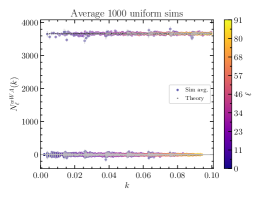
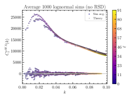
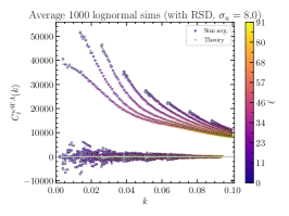
Figure 1: Here we show the SFB power spectrum for a full-sky survey with top-hat redshift bin $750\text{\,}{\mathrm{\text{$h$}}}^{-1}\text{\,}\mathrm{Mpc}1000\text{\,}{\mathrm{\text{$h$}}}^{-1}\text{\,}\mathrm{Mpc}$. In each panel the colored points show the simulations average with the color indicating the $\ell$-mode. Small black points indicate the theoretical calculation results. Left: Shot noise only; Center: Real-space lognormal simulations; Right: Redshift-space lognormal simulations. In all panels the SFB power spectrum modes separates into on-diagonal ($k=k^{\prime}$) and off-diagonal ($k\neq k^{\prime}$) modes. The off-diagonal modes cluster around zero power.

IV.2 FKP weights

The effect of adding arbitrary weights $w({\bm{r}})$, e.g., for optimizing the statistical power similar to Feldman et al. (1994) as in Eq. 7 is the following.

Since in the limit of infinitely many galaxies both the observed number density $n({\bm{r}})$ and the random catalog density $n_{r}({\bm{r}})$ are proportional the window $W({\bm{r}})$, Eq. 7 implies that the observed density contrast is related to the true underlying theoretical density contrast by

$$\delta^{\mathrm{obs}}=wW\delta\,.$$ (24)

However, the window $W({\bm{r}})$ and the weights $w({\bm{r}})$ enter the observed power spectrum differently. In particular, for the clustering signal we simply change $W\to wW$, e.g., in Eq. 19. On the other hand, the shot noise changes from $N\,\propto\,W$ to $N\,\propto\,w^{2}W$. We leave the detailed argument to Appendix B.

IV.3 Local average effect

The local average effect or integral constraint comes from measuring the number density of galaxies from the survey itself. This implies that the observed density contrast in the survey is measured relative to the average true density contrast. That is, $\delta^{\mathrm{obs}}({\bm{r}})\sim\delta({\bm{r}})-\bar{\delta}(z)$, where $\bar{\delta}(z)$ is the average density contrast in a thin redshift bin. This removes power from the largest angular scales. As a result the observed clustering and shot noise power spectra are given by four terms each

$$C^{wWA} =C^{1}-C^{23}-C^{4}\,,$$ (25)

$$N^{wWA} =N^{1}-N^{23}-N^{4}\,,$$ (26)

where the terms on the right-hand side are derived in Appendix C. In practice, all but the $C^{1}$ and $N^{1}$ terms essentially vanish for $\ell\gtrsim 2/f_{\mathrm{sky}}$.

IV.4 Pixel window

With our SuperFaB estimator only angular modes are affected by the HEALPix pixelization scheme Górski et al. (2005). We include the HEALPix pixel window in the theoretical modeling after the window and weights convolution, and before adding the shot noise, since shot noise is not affected by the pixel window.

V Validation with lognormal mocks

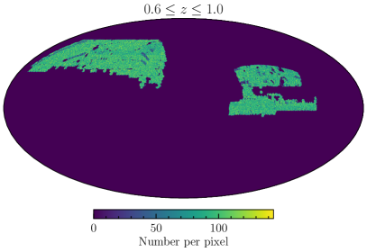
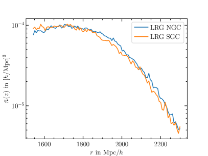
Figure 2: Catalog projection eBOSS DR16 LRGs. Left: angular projection at Healpix resolution $n_{\mathrm{side}}=256$. Right: radial selection function.

In this section we validate our pipeline using our own implementation of lognormal mocks (Coles and Jones, 1991; Xavier et al., 2016). Similar to Agrawal et al. (2017), our lognormals contain linear redshift space distortions, and optionally can have a large Gaussian FoG component.

We start with validating our model calculation on the full sky, then our window convolution and the importance of off-diagonal terms, local average effect, and boundary conditions.

V.1 Full-sky lognormal mocks

In Fig. 1 we start with a full-sky survey in the radial range $750\text{\,}{\mathrm{\text{$h$}}}^{-1}\text{\,}\mathrm{Mpc}1000\text{\,}{\mathrm{\text{$h$}}}^{-1}\text{\,}\mathrm{Mpc}$. The three panels compare our model described in Section IV to the average over $1000$ simulations; the first panel to the left compares the shot noise calculation with the estimator run on a uniform random data catalog; the center panel compares the model with a lognormal simulation in real space; the last panel compares the same in redshift space.

In each panel of Fig. 1, the color indicates the $\ell$-mode. Further, the modes broadly break into those that are on the diagonal $k=k^{\prime}$ and those that are off-diagonal. For the modes shown, the diagonal terms are all above $C_{\ell nn}\gtrsim$1000\text{\,}{\mathrm{\text{$h$}}}^{-3}\text{\,}{\mathrm{Mpc}}^{3}$$, while the off-diagonal $k\neq k^{\prime}$ terms are closer (but not necessarily equal) zero. Crucially, non-zero power is present in the off-diagonal terms even in real space.

V.2 eBOSS DR16 LRG lognormal mocks

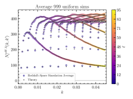
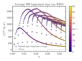
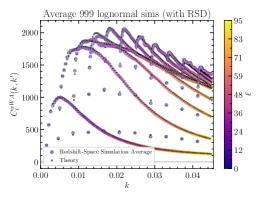
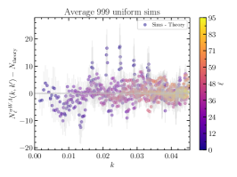
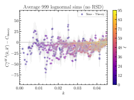
Figure 3: eBOSS-NGC-LRG-sky lognormal mocks. We only display $k=k^{\prime}$ ($\Delta n=0$) modes. The top row of panels displays the power spectrum for the three cases of uniform random mocks (left), lognormal mocks in real space (center), and lognormal mocks in redshift space (right). The bottom row displays the corresponding residuals to the theory.

$\Delta n_{\mathrm{max}}=0$: $\Delta n_{\mathrm{max}}=2$: $\Delta n_{\mathrm{max}}=4$:

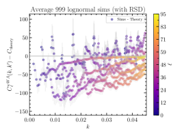
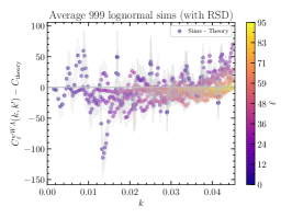
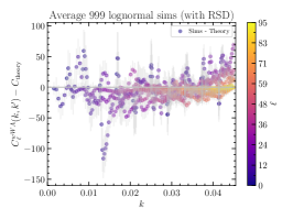
Figure 4: LRG-sky redshift-space lognormals. If the model is calculated only with on-diagonal modes ($k=k^{\prime}$, or $\Delta n=0$), then there is significant discrepancy between the simulation average and the theory model, as shown in the left panel. Even with just 2 off-diagonals included (center panel) the modeling is significantly improved. The right panel shows when modeling with up to $\Delta n_{\mathrm{max}}=4$ off-diagonals.

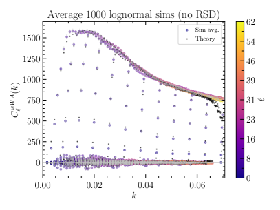
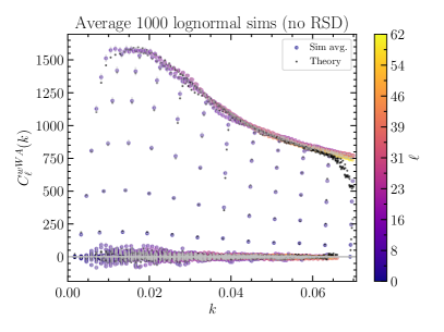
Figure 5: 1/16-th sky, constant radial selection between $500\text{\,}{\mathrm{\text{$h$}}}^{-1}\text{\,}\mathrm{Mpc}1000\text{\,}{\mathrm{\text{$h$}}}^{-1}\text{\,}\mathrm{Mpc}$. Left: theory local-average effect (LAE) calculation up to $\ell_{\mathrm{max}}\lesssim 16$. Right: theory LAE calculation up to $\ell_{\mathrm{max}}\lesssim 32$.

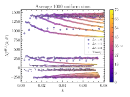
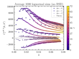
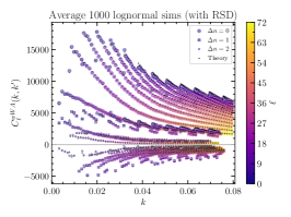
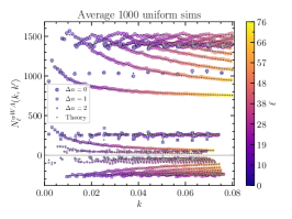
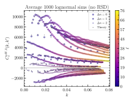
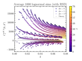
Figure 6: Comparison between potential (top) and velocity (bottom) boundary conditions with lognormal simulations for a thin shell covering half the sky. Top row shows the modes with potential boundaries that ensure a continuous and smooth field at the boundary, bottom row with velocity boundaries that set the vanishing velocity at the boundary.

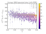
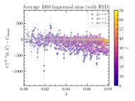
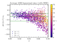
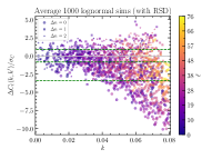
Figure 7: Left column shows the potential boundary modes, right column the velocity boundary modes, and the difference to our theory code for lognormal simulations with RSD. While the lognormals are afflicted by systematics, they are essentially the same whether potential or velocity boundaries are used. See right column of Fig. 6 for the absolute values of the modes.

Next, we validate our pipeline using the eBOSS DR16 LRG mask in the North Galactic Cap (NGC) and its radial selection function. The radial selection and angular windows are estimated from 1000 random catalogs provided by the SDSS collaboration (Zhao et al., 2021). Since we use the estimated window as the exact window for both generating and analysing the lognormal mocks, the details of this window-estimation procedure are irrelevant here, and we defer its description to Section VI.

Suffice to say that the resulting angular window encodes the fraction of each pixel that is observed. On the left of Fig. 2 we show the number of points in each pixel for the random catalog. Both NGC and SGC are shown. However, in this section we only use the NGC. The radial selection is shown on the right of Fig. 2, and it is estimated from the data catalog. We again defer the details to Section VI.

To ensure the presence of the local average effect (Section IV.3), we generate uniform random catalogs that match the radial number density distribution of each “data” catalog in the following way. For each redshift bin we draw exactly the same number of galaxies as in the data catalog. We adhere to the angular varying-depth window at that redshift by first uniformly drawing galaxies on the full sky, then rejecting points with probability proportional to the depth of the window. In this way a random catalog is created with the exact same redshift distribution as the data catalog (within the resolution of the analysis), and an angular distribution matching the angular window at each redshift.

We show our lognormal simulation results in Fig. 3, for uniform random data catalogs (left panels), real-space lognormals (center panels), and redshift-space lognormals (right panels). In addition to the observed power spectrum (convolved with window), we also show the difference to the calculated theory power spectrum. We get generally good agreement. The discrepancy at $k\gtrsim$0.04\text{\,}\mathrm{\text{$h$}}\text{\,}{\mathrm{Mpc}}^{-1}$$ comes from the incomplete window convolution that needs to make use of modes above our maximum $k_{\mathrm{max}}=$0.05\text{\,}\mathrm{\text{$h$}}\text{\,}{\mathrm{Mpc}}^{-1}$$ used in the analysis.

V.2.1 Importance of off-diagonal terms

In Fig. 3 we used off-diagonal $k_{n+\Delta n,\ell}\neq k_{n\ell}$ terms up to $\Delta n_{\mathrm{max}}=4$. As already mentioned for the full-sky case, these off-diagonal terms are important. We explicitly show this in Fig. 4, where we limit $\Delta n_{\mathrm{max}}=0$ (left panel), $\Delta n_{\mathrm{max}}=2$ (center panel), and $\Delta n_{\mathrm{max}}=4$ (right panel) for the redshift-space mocks. The figure shows that the on-diagonal $\Delta n=0$ terms are sufficiently modeled using $\Delta n_{\mathrm{max}}=2$. However, to model the off-diagonal terms as well, we conclude from Figs. 3 and 4 that for the eBOSS DR16 LRG redshift range and radial selection, $\Delta n_{\mathrm{max}}=4$ is needed and sufficient.

V.2.2 Local average effect modeling

Since the calculation for the local average effect in Appendix C is computationally expensive, we perform the calculation only up to some $\ell_{\mathrm{max}}$. In Fig. 5 we show the result when $\ell_{\mathrm{max}}=1/f_{\mathrm{sky}}$ and when it is $\ell_{\mathrm{max}}=2/f_{\mathrm{sky}}$. The residuals only become percent-level with the larger $\ell_{\mathrm{max}}$.

V.2.3 Potential vs. velocity boundaries

While potential boundaries have the property of being able to better model the density field with fewer modes, they have the unfortunate property that a sphere in real space does not stay a sphere in redshift space. Thus, our modeling in Section IV is technically inconsistent. However, those boundary effects are vanishingly small in the case of eBOSS DR16 LRGs, which we show in Fig. 6, where we compare with velocity boundary conditions (Fisher et al., 1995) that set the derivative to vanish on the boundaries, and, thus, a sphere in real space is also a sphere in redshift space. We show the derivation of the basis functions for velocity boundaries (including $k=0$ mode) in Appendix D.

To better assess if there is a relevant difference between the boundary conditions, Fig. 7 shows the difference between them. Since we use lognormal simulations that are inaccurate especially on small scales, we don’t expect the theory and measured average to agree perfectly. However, both potential and velocity boundaries show the same systematics. Thus, we conclude that the difference is insignificant.

VI Validation with EZmocks

To capture the full complexity of the eBOSS data, we use the EZmocks generated by Zhao et al. (2021). This allows us to test several potential sources of systematics that were not included in the lognormal mocks. First, we estimate the window from the 1000 random catalogs provided, and so the randoms are afflicted by a shot noise component. However, we find that this is negligible. Second, the complete EZmocks include redshift-evolution in the growth factor, galaxy bias, and radial dispersion (i.e., FoG and redshift uncertainty) that is lacking in the lognormal mocks. Third, the realistic EZmocks build on the complete EZmocks adding photometric systematics, fiber collisions, and redshift failures (Zhao et al., 2021; Ross et al., 2020; Raichoor et al., 2021; Gil-Marín et al., 2020; Neveux et al., 2020).

We match the cosmology to that used to create the EZmocks: a flat $\Lambda$CDM cosmology with $H_{0}=$67.77\text{\,}\mathrm{km}\text{\,}{\mathrm{s}}^{-1}\text{\,}{\mathrm{Mpc}}^{-1}$$ and $\Omega_{m}=0.307115$. In our fiducial cosmology the LRG redshift range $0.6\leq z\leq 1.0$ corresponds to radial distances $$1540$<\frac{r}{${\mathrm{\text{$h$}}}^{-1}\text{\,}\mathrm{Mpc}$}<$2467$$.

Our procedure for estimating the angular mask/window is as follows. We average over 1000 random catalogs provided by the SDSS collaboration (Zhao et al., 2021). At HEALPix resolution $n_{\mathrm{side}}=256$ and with 554 comoving distance bins, the number of random catalog points is added up for each voxel, to then estimate the number density in each voxel. The angular window is estimated by taking the mean over all redshift bins, and then normalizing. The angular footprint on sky is shown on the left of Fig. 2.

The radial selection function is estimated from the data in each cap separately. First, the data catalog is binned into 40 radial bins of width $\Delta z=0.01$, and then cubically splined. The radial selection function is shown on the right of Fig. 2.

VI.1 Complete EZmocks

Slice 1: $z=0.6-0.645$
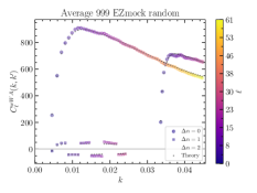
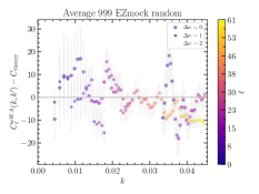
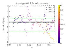
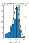
Slice 2: $z=0.655-0.695$
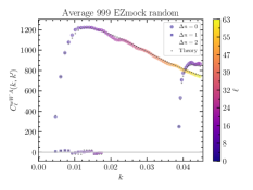
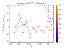
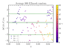
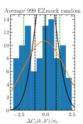
Slice 3: $z=0.705-0.795$
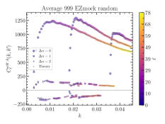
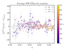
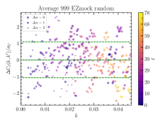
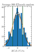
Slice 4: $z=0.805-0.895$
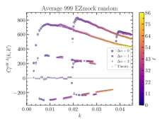
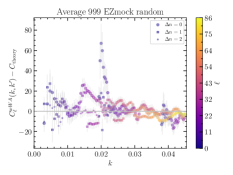
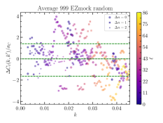
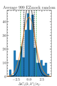
Slice 5: $z=0.905-1.0$

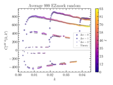
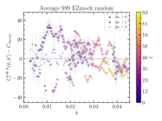
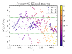
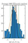
Figure 8: Each row shows the SFB power spectrum measured in each of the redshift slices used to generate the LRG EZmocks in the NGC. We show the full SFB power spectrum in the slice in the left panels, the residual relative to the theory in the center left panels, the same residual rescaled by the standard deviation as measured from the simulations in the center right panels, and a histogram of those standard-deviation-rescaled residuals in the left panels. In the two right-most columns the green dashed lines are the 16, 50, and 84 percentiles. In the right-most column we also show in orange a Gaussian fit, in black solid a Gaussian of unity width with black dashed lines as the corresponding 16, 50, and 84 percentiles. We adjusted the bias parameters to fit each slice. We added a buffer of $\Delta z=0.05$ to each slice in order to avoid leakage due to RSD from neighboring slices.

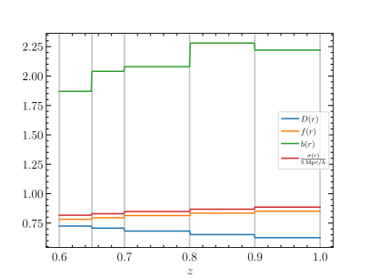
Figure 9: eBOSS DR16 LRG growth factor, growth rate, bias, and FoG evolution.

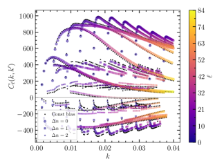
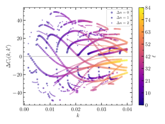
Figure 10: The SFB power spectrum is sensitive to redshift evolution, as exemplified here by comparing the SFB power spectrum with the biases for the 5 redshift slices set equal (black points) with the step-function bias (larger colored points). Both are the theoretical curves.

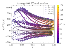
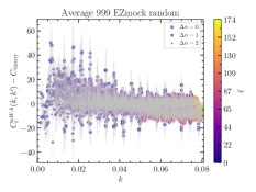
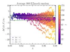
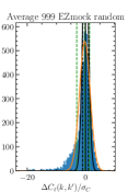
Figure 11: This figure is similar to Fig. 8, except that now the full redshift range over all five slices of the complete LRG NGC EZmocks is used. Without any further fitting of bias and cosmological parameters compared to Fig. 8, we get generally good agreement between the mocks’ average and theory, with a significant discrepancy only on smaller scales, as seen in the center right panel.

To model the evolution of structure and galaxy bias with redshift, the EZmock catalogs for the LRG sample are generated in 5 redshift slices (Zhao et al., 2021). We show SFB measurements from each of these slices in Fig. 8. In order to avoid leakage due to RSD from neighboring slices we chose redshift slices that are thinner by $\Delta z=0.05$ on each side than the original slices used to generate the mocks.

For each redshift slice, the left column of Fig. 8 shows the average over 999 complete EZmock simulations and a theory curve where the linear galaxy bias was adjusted to fit the measurement in that slice. The center left column shows the residuals with the error bars estimated from the 999 EZmocks. The center right column shows the residuals relative to the standard deviation of that mode, ignoring mode-couplings, and dashed horizontal lines indicating the 16th, 50th, and 84th percentiles. The left-most column shows a histogram of those relative residuals as well as a Gaussian fit in orange, and a standard Gaussian in black.

Slices 1 and 2 cover a smaller redshift range and, thus, have fewer modes (and no $\Delta n=2$ modes). Modes are also coupled due to the limited sky coverage, so that the number of degrees of freedom is fairly small, and slice 2, in particular, is quite noisy. Slice 3 contains the most galaxies, and the 16th, 50th, and 84th percentiles are nearly exactly coincident with the 1-$\sigma$ lines.

The linear galaxy biases thus obtained are plotted as step-functions in Fig. 9.

The sensitivity of the SFB power spectrum to the evolution of the linear galaxy bias $b(z)$ is shown in Fig. 10, where we compare theory curves for constant bias and the step-function bias. The difference is on the level of $\sim 5\text{\,}\mathrm{\char 37\relax}$.

Using the bias model in Fig. 9, we now show the comparison with the complete EZmocks with all 5 redshift slices in Fig. 11. In the figure, we extend the range of modes up to $k_{\mathrm{max}}=$0.1\text{\,}\mathrm{\text{$h$}}\text{\,}{\mathrm{Mpc}}^{-1}$$. However, we only show up to $k=$0.08\text{\,}\mathrm{\text{$h$}}\text{\,}{\mathrm{Mpc}}^{-1}$$ because of the incomplete window convolution above that.

As Fig. 11 shows, the model is unbiased on large scales. However, small angular modes with high $\ell$ (yellow points in the figure) are significantly biased relative to their covariance. This comes from the fact that we measured the radial selection function from the data which is afflicted by systematics that are not present in the complete EZmocks. We remedy this situation with the realistic EZmocks in the next section.

VI.2 Realistic EZmocks

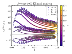
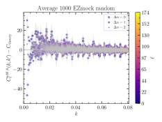
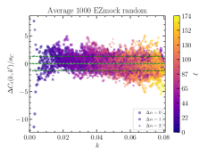
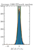
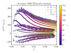
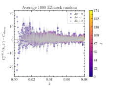
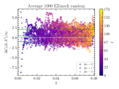
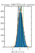
Figure 12: This figure is similar to Fig. 11, except that here we used the realistic EZmocks that include systematics, and we have also included FKP weights in the power spectrum estimation. Furthermore, the top row of panels shows the comparison between mocks’ average and theory for the NGC, and the bottom row for the SGC. The same cosmological and bias parameters were used for NGC and SGC.

Several observational systematics enter the analysis of the eBOSS DR16 ELG samples. Building ontop of the complete EZmocks, the realistic EZmocks add the effects of photometric systematics, close-pair fiber collisions, and redshift failures. Weights to correct for these systematics are provided by the EZmocks.

In addition to the systematic weights we apply FKP weights according to Eq. 6. We chose to apply our own FKP weights instead of those provided by EZmocks, for no other than practical reasons, e.g., to apply them to our lognormal simulations.

Fig. 12 shows the average over the 1000 EZmocks for the NGC in the top panels and for the SGC in the bottom panels of the figure. The simulations and data analysis are fully consistent with each other, and the agreement is within the statistical expectation for both NGC and SGC.

VII MCMC fitting and Covariance matrix

In this section we test our likelihood construction and MCMC fitting. The covariance matrix is estimated from 1000 realistic EZmocks (Zhao et al., 2021). We briefly describe how we invert such a noisy covariance matrix using the eigenvector method outlined in Wang et al. (2020), and then we apply that to a few realizations of the EZmocks.

Assuming the SFB power spectrum modes are Gaussian distributed, we construct the likellihood as follows.

$$-2\ln\mathcal{L} =\mathrm{const}+(\hat{C}-C)^{T}M^{-1}(\hat{C}-C)\,,$$ (27)

where $\hat{C}$ is the vector of measured $C_{\ell nn^{\prime}}$ values, $C$ is the SFB power spectrum model and $M$ is the covariance matrix.

VII.1 On the inversion of noisy convariance matrices

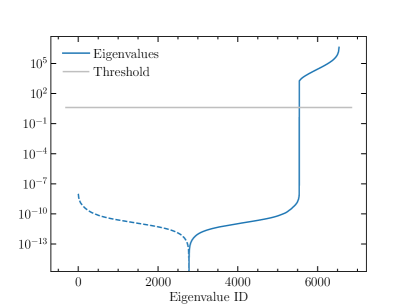
Figure 13: Eigenvalues of the full covariance matrix estimated from 1000 EZmocks, sorted from smallest to largest, dashed means negative. The largest 1000 eigenvalues are well-constrained. The smaller eigenvales are consistent with numerical machine-level noise around a mean of zero. The grey line indicates the cutoff for which we use eigenvalues in the matrix inversion.

A covariance matrix estimated from simulations is afflicted by noise. In our case, the number of modes exceeds the number of simulations. Thus, only 1000 eigenvalues of the covariance matrix are measured from the 1000 simulations, and the rest are zero within machine precision. An example is shown in Fig. 13.

Therefore, the inverse of the measured covariance matrix will be dominated by the noise of the unmeasured eigenvalues. To solve this we use the approach outlined in Wang et al. (2020) that ensures that the inverted matrix is dominated by well-constrained eigenmodes. The assumption is that the eigenvectors with large eigenvalues are the best determined. Thus, only the eigenvectors with the largest eigenvalues are retained.

There are a few unfortunate consequences of this approach. First, the modes that have a small variance and, thus, would contribute most to the likelihood are thrown away. However, here we are interested in the largest scales, and these modes tend to have larger uncertainties due to the limited volume in the survey. Thus, we expect these large modes to be retained in this approach. Second, among the modes with large uncertainties, the noise in the covariance estimate means that there is some stochasticity as to the exact modes that get retained. Some modes will be over estimated, and those will definitely be retained, which merely degrades the constraints. However, it is also possible (e.g., if the numbers of modes is similar to the number of simulations) that some covariance entries get underestimated, in which case we could get biased constraints. We leave a more detailed investigation to a future paper.

The inversion works essentially as a lossy compression algorithm. First, the variable condition number of an eigenmode $i$ is defined as

$$\varrho_{i} =\frac{\lambda_{\mathrm{max}}}{\lambda_{i}}\,,$$ (28)

where $\lambda_{1}\leq\ldots\leq\lambda_{N}=\lambda_{\mathrm{max}}$ are the eigenvalues sorted from smallest to largest. We then keep only the largest eigenvectors starting at the smallest $i_{\mathrm{min}}$ such that $\varrho_{i_{\mathrm{min}}}\geq\varrho_{\mathrm{threshold}}=1000$. The compression matrix $R$ is then constructed from these $J=N-i_{\mathrm{min}}+1$ eigenvectors $\bm{e}_{j}$,

$$R =(\bm{e}_{i_{\mathrm{min}}},\ldots,\bm{e}_{N})^{\dagger}\in\mathbb{C}^{J\times N}\,,$$ (29)

which satisfies $RR^{\dagger}=1$. Then, the compressed data vector is

$$\Delta =R\delta\,,$$ (30)

and the compressed covariance matrix is

$$C =RMR^{\dagger}\,,$$ (31)

which is positive-definite if $M$ is positive-definite. The likelihood analysis is then performed in compressed space with data vector $\Delta$ and covariance matrix $C$.

Wang et al. (2020) have shown that the matrix $R$ can be recycled between iterations of the MCMC fitting procedure as long as the parameter space that is being explored stays in a similar region.

VII.2 MCMC fitting

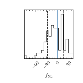
Figure 14: Histogram of best-fit $f_{\mathrm{NL}}$ for 100 simulations. The blue line marks the fiducial $f_{\mathrm{NL}}=0$, the dashed lines the 16th and 84th percentiles.

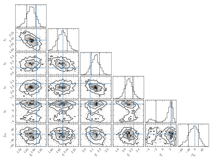
Figure 15: MCMC results for a single EZmock. The blue crosses mark the fiducial value as measured from all EZmocks, the orange point marks the point that had the highest likelihood in the chain. All parameters except the bias $b_{4}$ for the highest redshift slice are reasonably well constrained and consistent with the fiducial.

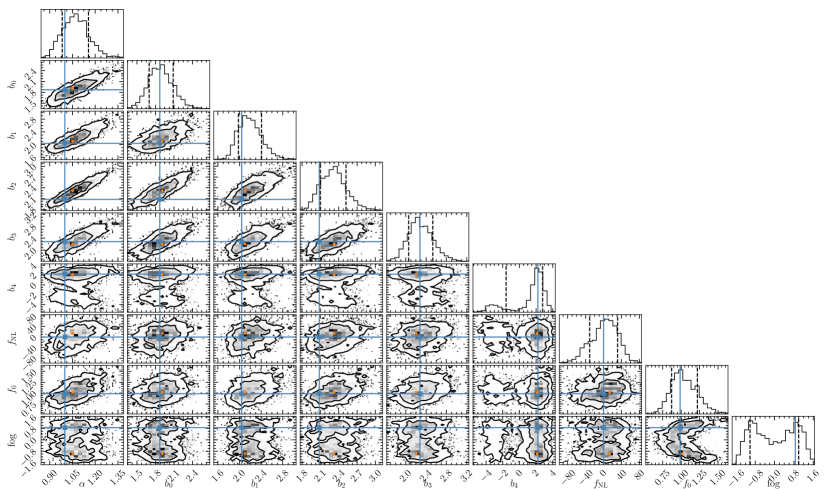
Figure 16: Similar to Fig. 15, except with additional parameters for RSD, FoG, and Alcock-Paczynski.

As a final step in this auto-correlation SFB validation paper, we use single EZmock simulations as data. First, we will measure the bias parameters and $f_{\mathrm{NL}}$ from the average of the simulations, then we include RSD, FoG and single-parameter Alcock-Paczynski.

For our MCMC we developed in Julia an adaptive Metropolis-Hastings sampler (Roberts and Rosenthal, 2009). Adaptive here means that the covariance matrix of the proposal distribution is updated every few steps. Therefore, the chain is Markovian only asymptotically in the limit of a large number of steps. We use the following procedure to get a robust estimate of the errors. The number of steps is a multiple of $M=n(n+1)$, where $n$ is the number of parameters. We first run the chain for $100M$ steps to get an estimate for the maximum likelihood point. Then, we run it again for $100M$ points to get an estimate of the covariance matrix for the parameters. We then run it twice more, each time updating both the starting point with the new maximum lileklihood point and the initial covariance matrix. Finally, we run the adaptive Metropolis-Hastings sampler for $700M$ steps, and these samples will be the ones used as output of the MCMC.

Fig. 14 shows a histogram over 100 sims, fitting only $f_{\mathrm{NL}}$ and keeping all other parameters constant. We used only the NGC, and $\ell\geq 4$, and $k_{\mathrm{max}}=$0.08\text{\,}\mathrm{\text{$h$}}\text{\,}{\mathrm{Mpc}}^{-1}$$. While the noise is large, the set of ensembles is consistent with $f_{\mathrm{NL}}=0$, as we would expect given the input simulations.

Fig. 15 shows an MCMC run with the 5 biases (one for each redshift slice) and $f_{\mathrm{NL}}$ as parameters. The measured bias parameters are essentially the same as when we fix $f_{\mathrm{NL}}=0$, and they are consistent with the average measured from all EZmocks in Section VI.1, generally within the $68\text{\,}\mathrm{\char 37\relax}$ contours.

Finally, Fig. 16 shows an MCMC run for the 5 biases, $f_{\mathrm{NL}}$, Kaiser parameter $f_{0}$, FoG $\sigma_{u}$, and Alcock-Paczynski parameter $\gamma$. The FoG parameter only enters as its square, hence negative values are equally allowed.

While the error contours are large, they are largely unbiased. Crucially, the EZmocks were created with $f_{\mathrm{NL}}=0$, and we successfully recover that from the simulations.

VIII Conclusion

In this paper we validate our pipeline for using the SuperFaB estimator for cosmological inference on the spherical Fourier-Bessel pseudo power spectrum. We develop a reasonably fast SFB power spectrum calculator along the lines of Khek et al. (2022). We derive in detail the shot noise and the local average effect with weights.

We start the validation with full-sky lognormal simulations in real and redshift space (similar to Agrawal et al., 2017), and then progressively add redshift-space distortions, realistic masks, radial selection, and systematic weights using the EZmocks of Zhao et al. (2021). We also verify the use of potential and velocity boundary conditions.

We model the EZmocks bias prescription by steps as shown in Fig. 9. For the NGC and SGC separately, we verify that the model including all systematics is consistent with the measured modes of the EZmocks, Fig. 12.

Finally, we construct a Gaussian likelihood for the power spectrum, we measure the covariance matrix from all $1000$ EZmocks with a large-eigenvalue-inversion, and we verify that the measured $f_{\mathrm{NL}}$ from 100 EZmocks is consistent with zero, Fig. 14, and that all the parameters of the model are consistent with their fiducial values.

For the future we plan to apply the method on the data, improve the covariance estimate, and develop the multi-tracer SFB analysis.

Appendix A Useful formulae

Spherical Bessel functions and spherical harmonics satisfy orthogonality relations

$$\delta^{D}(k-k^{\prime}) =\frac{2kk^{\prime}}{\pi}\int_{0}^{\infty}\mathrm{d}{r}\,r^{2}\,j_{\ell}(kr)\,j_{\ell}(k^{\prime}r)\,,$$ (32)

$$\delta^{K}_{\ell\ell^{\prime}}\delta^{K}_{mm^{\prime}} =\int\mathrm{d}{\Omega}_{{\hat{\bm{r}}}}\,Y_{\ell m}({\hat{\bm{r}}})\,Y^{*}_{\ell^{\prime}m^{\prime}}({\hat{\bm{r}}})\,.$$ (33)

The Laplacian in spherical coordinates is

$$\nabla^{2}f =\frac{1}{r^{2}}\,\frac{\partial}{\partial r}\left(r^{2}\,\frac{\partial f}{\partial r}\right)+\frac{1}{r^{2}\sin\theta}\,\frac{\partial}{\partial\theta}\left(\sin\theta\,\frac{\partial f}{\partial\theta}\right)$$

$$\quad+\frac{1}{r^{2}\sin^{2}\theta}\,\frac{\partial^{2}f}{\partial\phi^{2}}\,.$$ (34)

The SFB transform pair is

$$\delta({\bm{r}}) =\int\mathrm{d}k\,\sum_{\ell m}\left[\sqrt{\frac{2}{\pi}}\,k\,j_{\ell}(kr)\,Y_{\ell m}(\theta,\phi)\right]\delta_{\ell m}(k)\,,$$ (35)

$$\delta_{\ell m}(k) =\int\mathrm{d}^{3}r\left[\sqrt{\frac{2}{\pi}}\,k\,j_{\ell}(kr)\,Y^{*}_{\ell m}({\hat{\bm{r}}})\right]\delta({\bm{r}})\,.$$ (36)

Appendix B Shot noise and FKP Weighting

Here we consider the effect of the weighting on the clustering signal and shot noise. We start with the Poisson statistics of the sampled field (Peebles, 1973; Feldman et al., 1994)

$$\left\langle n({\bm{r}})\,n({\bm{r}}^{\prime})\right\rangle =\bar{n}({\bm{r}})\,\bar{n}({\bm{r}}^{\prime})\left[1+\xi({\bm{r}},{\bm{r}}^{\prime})\right]$$

$$\quad+\bar{n}({\bm{r}})\,\delta^{D}({\bm{r}}-{\bm{r}}^{\prime})\,,$$ (37)

$$\alpha\left\langle n({\bm{r}})\,n_{r}({\bm{r}}^{\prime})\right\rangle =\bar{n}({\bm{r}})\,\bar{n}({\bm{r}}^{\prime})\,,$$ (38)

$$\alpha^{2}\left\langle n_{r}({\bm{r}})\,n_{r}({\bm{r}}^{\prime})\right\rangle =\bar{n}({\bm{r}})\,\bar{n}({\bm{r}}^{\prime})$$

$$\quad+\alpha\,\bar{n}({\bm{r}})\,\delta^{D}({\bm{r}}-{\bm{r}}^{\prime})\,,$$ (39)

where $n({\bm{r}})$ is the number density of the data catalog, $n_{r}({\bm{r}})$ that of the random catalog, and we define ${\bar{n}}({\bm{r}})=\left\langle n({\bm{r}})\right\rangle=\alpha\left\langle n_{r}({\bm{r}})\right\rangle$, and $\alpha$ is the ratio of the number of points in the data catalog to the number of points in the random catalog. With Eq. 7 the correlation function becomes

$$\left\langle\delta^{\mathrm{obs}}({\bm{r}})\,\delta^{\mathrm{obs}}({\bm{r}}^{\prime})\right\rangle =w({\bm{r}})w({\bm{r}}^{\prime})W({\bm{r}})\,W({\bm{r}}^{\prime})\,\xi({\bm{r}},{\bm{r}}^{\prime})$$

$$\quad+(1+\alpha)\,\frac{w^{2}({\bm{r}})W({\bm{r}})\,\delta^{D}({\bm{r}}^{\prime}-{\bm{r}})}{\bar{n}}\,,$$ (40)

where we used the window function $W({\bm{r}})={\bar{n}}({\bm{r}})/{\bar{n}}$, which is how we define it throughout the paper. Eq. 40 shows that there is a difference between the window and the weighting. This difference appears in the shot noise term, which must still include the square of the weighting function, but contains the window only linearly.

The SFB transform of the shot noise term becomes (i.e., Eq. 2)

$$N^{\mathrm{obs}} =\frac{1+\alpha}{\bar{n}}\,\mathrm{SFB}^{2}[w^{2}({\bm{r}})W({\bm{r}})\delta^{D}({\bm{r}}^{\prime}-{\bm{r}})]$$ (41)

$$=\frac{1+\alpha}{\bar{n}}\,(w^{2}W)_{n\ell m}^{n^{\prime}\ell^{\prime}m^{\prime}}\,,$$ (42)

where our notation $(w^{2}W)$ signifies the window convolution matrix Section IV.1, but with $W\to w^{2}W$. The pseudo-power shot noise is

$$N_{\ell nn^{\prime}}^{\mathrm{obs}} =\frac{1+\alpha}{{\bar{n}}}\,\frac{1}{\sqrt{4\pi}}\,\int\mathrm{d}r\,r^{2}\,g_{n\ell}(r)\,g_{n^{\prime}\ell}(r)\,(w^{2}W)_{00}(r)\,.$$ (43)

Eq. 40 also shows that the coupling matrix is modified by calculating it with the substitution $W({\bm{r}})\to w({\bm{r}})W({\bm{r}})$.

In summary, the following changes are introduced by the weighting:

1. In the estimator, each galaxy needs to be multiplied by the weight $w({\bm{r}})$ at its location, see Section III. (If no random catalog is used, then this also means that $W_{\ell n}({\hat{\bm{r}}})$ must be calculated with the substitution $W({\bm{r}})\to w({\bm{r}})W({\bm{r}})$.)

2. The coupling matrix is computed with the substitution $W({\bm{r}})\to w({\bm{r}})W({\bm{r}})$.

3. The shot noise is calculated with the substitution $W({\bm{r}})\to w^{2}({\bm{r}})W({\bm{r}})$.

4. The local average effect changes as a result of the weighting, and we defer the details to Appendix C.

Appendix C Local Average Effect with weighting

In this section we recognize that the average number density ${\bar{n}}$ in Eq. 7 must in practice be measured from the survey itself. This is often called the integral constraint (Beutler et al., 2014; de Mattia and Ruhlmann-Kleider, 2019) or the local average effect (de Putter et al., 2012; Wadekar et al., 2020).

Compared to Grasshorn Gebhardt and Doré (2021) we include a weighting $w({\bm{r}})$. We also consider an extension where ${\bar{n}}(z)$ is independently determined at every redshift (de Mattia and Ruhlmann-Kleider, 2019).

Measuring the average number density is accomplished by dividing the total number of galaxies in the survey (or the total number in each redshift bin) by the effective volume. However, the total number of galaxies in the survey is a stochastic quantity such that the average number density is given by

$${\bar{n}} =\left(1+\bar{\delta}\,\right){\bar{n}}^{\mathrm{true}}\,,$$ (44)

where ${\bar{n}}^{\mathrm{true}}$ is the true density contrast if one were to measure on a much larger survey volume. Defining the effective volume

$$V_{\mathrm{eff}} =\int\mathrm{d}^{3}r\,W({\bm{r}})\,,$$ (45)

the average density contrast within the survey volume is

$$\bar{\delta} =\frac{1}{V_{\mathrm{eff}}}\int\mathrm{d}^{3}{\bm{r}}\,W({\bm{r}})\,\delta({\bm{r}})\,,$$ (46)

or, if we measure the number density as a function of redshift,

$$\bar{\delta}(z) =\frac{1}{4\pi f^{\mathrm{eff}}_{\mathrm{sky}}(z)}\int\mathrm{d}^{2}\hat{r}\,W({\bm{r}})\,\delta({\bm{r}})\,,$$ (47)

where we define the effective sky fraction as

$$f^{\mathrm{eff}}_{\mathrm{sky}}(z) =\frac{1}{4\pi}\int\mathrm{d}^{2}\hat{r}\,W({\bm{r}})\,.$$ (48)

That is, we fold the radial selection $\phi(z)$ into the effective sky fraction. Next, we define the triplet $\mu=(n_{\mu},\ell_{\mu},m_{\mu})$. Then, the average density field in SFB space becomes

$$\bar{\delta}_{\mu} =\delta^{K}_{\ell_{\mu}0}\delta^{K}_{m_{\mu}0}\begin{cases}V_{\mathrm{eff}}^{-1}\,d_{\mu}d^{*}_{\nu}\,W_{\nu\rho}\delta_{\rho}&\text{ for }\bar{\delta}=const\,,\\ \widetilde{W}_{\mu\rho}\delta_{\rho}&\text{ for }\bar{\delta}=\bar{\delta}(z)\,,\end{cases}$$ (49)

where we sum over repeated indices and we defined the SFB transform of a unit uniform field,

$$d_{\mu} =\sqrt{4\pi}\,\delta^{K}_{\ell_{\mu}0}\delta^{K}_{m_{\mu}0}\int\mathrm{d}r\,r^{2}\,g_{n_{\mu}0}(r)\,,$$ (50)

and

$$\widetilde{W}_{\mu\rho} =\int\mathrm{d}^{3}r\,g_{\mu}(r)\,g_{\rho}(r)\,Y^{*}_{\mu}({\hat{\bm{r}}})\,Y_{\rho}({\hat{\bm{r}}})\,\frac{W({\bm{r}})}{f^{\mathrm{eff}}_{\mathrm{sky}}(z)}\,,$$ (51)

which is the mixing matrix if the window is $W/f^{\mathrm{eff}}_{\mathrm{sky}}$ (e.g., Eq. (34) in Grasshorn Gebhardt and Doré, 2021). If the window is separable, then $W/f^{\mathrm{eff}}_{\mathrm{sky}}$ is purely a function of ${\hat{\bm{r}}}$, and $\widetilde{W}$ is proportional the coupling matrix due to the angular window. The Kronecker-deltas in Eq. 49 ensure that $\widetilde{W}$ only needs to be calculated for $\ell_{\mu}=m_{\mu}=0$, and it describes the coupling of the angular DC mode to the higher multipoles for a partial sky.

With our model in Eq. 7, the measured density contrast is (similar to Taruya et al., 2021)

$$\delta^{\mathrm{obs}}({\bm{r}})\equiv\delta^{wWA}({\bm{r}}) =w({\bm{r}})\,W({\bm{r}})\,\frac{\delta({\bm{r}})-\bar{\delta}}{1+\bar{\delta}}\,,$$ (52)

where $\delta({\bm{r}})$ is the true density contrast, the superscript ‘A’ refers to the local average effect, and the superscript ‘W’ refers to the effect of the window convolution.

The SFB transform of Eq. 52 is

$$\delta^{wWA}_{\mu} \simeq(wW)_{\mu\rho}\,[\delta_{\rho}-\bar{\delta}_{\rho}]\,,$$ (53)

to first order in $\bar{\delta}$, and we defined the mixing matrix $(wW)_{\mu\rho}=w_{\mu\sigma}W_{\sigma\rho}$.

The observed weighted correlation function is

$$\left\langle\delta^{wWA}_{\mu}\delta^{wWA,*}_{\nu}\right\rangle =(wW)_{\mu\rho}\Big{[}\left\langle\delta_{\rho}\delta^{*}_{\lambda}\right\rangle-\left\langle\delta_{\rho}\bar{\delta}^{*}_{\lambda}\right\rangle$$

$$\quad-\left\langle\bar{\delta}_{\rho}\delta^{*}_{\lambda}\right\rangle+\left\langle\bar{\delta}_{\rho}\bar{\delta}^{*}_{\lambda}\right\rangle\Big{]}(wW)_{\lambda\nu}\,,$$ (54)

where we used that the mixing matrix is Hermitian, $(wW)^{*}_{\kappa\lambda}=(wW)_{\lambda\kappa}$.

Appendix C contains four terms. The first term is the clustering term,

$$P^{1}_{\mu\nu} =(wW)_{\mu\rho}\left\langle\delta_{\rho}\delta^{*}_{\lambda}\right\rangle(wW)_{\lambda\nu}\,.$$ (55)

The other terms in Appendix C we call $P^{2}_{\mu\nu}$, $P^{3}_{\mu\nu}$, and $P^{4}_{\mu\nu}$ with similar definitions as $P^{1}_{\mu\nu}$, and they are due to the local average effect. The second and third terms are related by taking the adjoint. That is,

$$P^{3}_{\mu\nu} =(wW)_{\mu\rho}\left\langle\bar{\delta}_{\rho}\delta^{*}_{\lambda}\right\rangle(wW)_{\lambda\nu}=P^{2,*}_{\nu\mu}\,.$$ (56)

The second and third terms are the computationally most expensive to calculate. The reason is that the correlation between the two isotropic fields $\delta({\bm{r}})$ and $\bar{\delta}(r^{\prime})$ comes from the anisotropic region on the partial sky defined by the window function. Thus, the correlation $\left\langle\delta({\bm{r}})\bar{\delta}(r^{\prime})\right\rangle$ is anisotropic, and this couples $\ell=0$ modes with higher-$\ell$ modes. Hence, treating $\left\langle\delta_{\rho}\bar{\delta}^{*}_{\lambda}\right\rangle$ as a pseudo-power spectrum with $(\ell_{\rho},m_{\rho})=(\ell_{\lambda},m_{\lambda})$ is inadequate, in general. However, we use the heuristic that only modes up to $\ell_{\rho}\lesssim 1/(2f_{\mathrm{sky}})$ couple to $\ell_{\lambda}=0$, since that is approximately the width of the window function in spherical harmonic space.

We treat the clustering and shot noise terms separately so that $P^{i}=C^{i}+N^{i}$. We define the observed weighted power spectrum and shot noise as

$$C^{wW}_{\mu\nu} =(wW)_{\mu\sigma}C_{\sigma\rho}(wW)_{\rho\nu}\,,$$ (57)

$$N^{wW}_{\sigma\rho} =\frac{1}{{\bar{n}}}\,(w^{2}W)_{\sigma\rho}=\frac{1}{{\bar{n}}}\,w_{\sigma\alpha}W_{\alpha\beta}w_{\beta\rho}\,,$$ (58)

where $C_{\sigma\rho}$ enforces the isotropy condition $\ell_{\sigma}=\ell_{\rho}$ and $m_{\sigma}=m_{\rho}$, and the shot noise is from Eq. 42. Then,

$$P^{1}_{\mu\nu} =C^{wW}_{\sigma\rho}+N^{wW}_{\mu\nu}\,.$$ (59)

To calculate the local average effect terms we treat them in two different ways, depending on whether we consider a constant $\bar{\delta}$ or $\bar{\delta}(z)$. In either case, the result can be separated into clustering and shot noise terms. Furthermore, we will only consider the pseudo-SFB power spectrum.

C.1 Constant average density contrast

Considering a constant $\bar{\delta}$, the result will be written as the matrix equations

$$C^{wWA} =C^{wW}-\widetilde{T}C+\mathrm{tr}(C^{W}D)\,D^{wW}\,,$$ (60)

$$N^{wWA} =N^{wW}-[2{\bar{n}}^{-1}-\mathrm{tr}(N^{W}D)]\,D^{wW}\,,$$ (61)

where $\widetilde{T}$ is given in Eq. 74. The traces are given in Eqs. 78 and 79, and $D^{wW}$ can be calculated efficiently, as shown in Grasshorn Gebhardt and Doré (2021).

Next, we calculate the second term in Appendix C assuming constant $\bar{\delta}$. Using Eq. 49, we write

$$P^{2}_{\mu\nu} =w_{\mu\sigma}W_{\sigma\rho}\left\langle\delta_{\rho}\bar{\delta}^{*}_{\lambda}\right\rangle W_{\lambda\kappa}w_{\kappa\nu}$$ (62)

$$=V_{\mathrm{eff}}^{-1}w_{\mu\sigma}[C^{W}_{\sigma\iota}+N^{W}_{\sigma\iota}]d_{\iota}d^{*}_{\lambda}W_{\lambda\kappa}w_{\kappa\nu}$$

$$=V_{\mathrm{eff}}^{-1}w_{\mu\sigma}[C^{W}_{\sigma\iota}+N^{W}_{\sigma\iota}]d_{\iota}d^{wW,*}_{\nu}$$

$$=V_{\mathrm{eff}}^{-1}w_{\mu\sigma}C^{W}_{\sigma\iota}d_{\iota}d^{wW,*}_{\nu}+{\bar{n}}^{-1}D^{wW}_{\mu\nu}$$

$$=V_{\mathrm{eff}}^{-1}(wW)_{\mu\rho}[C_{\rho\omega}W_{\omega\iota}d_{\iota}d^{*}_{\lambda}](wW)_{\lambda\nu}+{\bar{n}}^{-1}D^{wW}_{\mu\nu}\,,$$ (63)

where we used that $N^{W}_{\sigma\iota}={\bar{n}}^{-1}W_{\sigma\iota}$, and $(wW)_{\mu\rho}$ is the mixing matrix for $w({\bm{r}})W({\bm{r}})$, and we defined

$$D^{wW}_{\mu\nu} =(wW)_{\mu\alpha}\,D_{\alpha\beta}\,(wW)_{\beta\nu}\,,$$ (64)

along with

$$D_{\alpha\beta} =d_{\alpha}\,d^{*}_{\beta}\,.$$ (65)

The term in brackets is

$$[C_{\rho\omega}W_{\omega\iota}d_{\iota}d^{*}_{\lambda}] =\sum_{n_{\omega}}C_{\ell_{\rho}n_{\rho}n_{\omega}}W_{n_{\omega}\ell_{\rho}m_{\rho}}\,d_{\lambda}\,,$$ (66)

where we used

$$d_{n\ell m}^{W} =\sum_{n^{\prime}}W_{n\ell m}^{n^{\prime}00}d_{n^{\prime}00}$$ (67)

$$=\int\mathrm{d}r\,r^{2}\,g_{n\ell}(r)\,W_{\ell m}(r)\int\mathrm{d}r^{\prime}\,r^{\prime 2}\sum_{n^{\prime}}g_{n^{\prime}0}(r)\,g_{n^{\prime}0}(r^{\prime})$$

$$=W_{n\ell m}\,,$$ (68)

and the last step follows from the orthogonality of the basis functions in harmonic space, $\sum_{n}g_{n0}(r)g_{n0}(r^{\prime})=r^{-2}\delta^{D}(r-r^{\prime})$. Thus, we get

$$P^{2}_{\mu\nu} =C^{2,wW}_{\mu\nu}+{\bar{n}}^{-1}D^{wW}_{\mu\nu}\,,$$ (69)

where

$$C^{2,wW}_{\mu\nu} =(wW)_{\mu\rho}\left[V_{\mathrm{eff}}^{-1}\sum_{n_{\omega}}C_{\ell_{\rho}n_{\rho}n_{\omega}}W_{n_{\omega}\ell_{\rho}m_{\rho}}\,d_{\lambda}\right](wW)_{\lambda\nu}$$ (70)

$$=V_{\mathrm{eff}}^{-1}\sum_{n_{\rho}\ell_{\rho}m_{\rho}}(wW)_{n_{\mu}\ell_{\mu}m_{\mu}}^{n_{\rho}\ell_{\rho}m_{\rho}}\sum_{n_{\omega}}W_{n_{\omega}\ell_{\rho}m_{\rho}}C_{\ell_{\rho}n_{\rho}n_{\omega}}$$

$$\quad\times(wW)^{*}_{n_{\nu}\ell_{\nu}m_{\nu}}\,,$$ (71)

where the last line follows again from Eq. 68 and the Hermitian property of $(wW)_{\lambda\nu}$. For the pseudo-power spectrum we set $(\ell_{\mu},m_{\mu})=(\ell_{\nu},m_{\nu})$, and average over $m_{\mu}$,

$$C^{2,wW}_{\ell_{\mu}n_{\mu}n_{\nu}} =\sum_{\ell_{\rho}n_{\rho}n_{\omega}}T_{\ell_{\mu}n_{\mu}n_{\nu}}^{\ell_{\rho}n_{\rho}n_{\omega}}\,C_{\ell_{\rho}n_{\rho}n_{\omega}}\,,$$ (72)

where

$$T_{\ell_{\mu}n_{\mu}n_{\nu}}^{\ell_{\rho}n_{\rho}n_{\omega}} =\frac{1}{V_{\mathrm{eff}}\left(2\ell_{\mu}+1\right)}\sum_{m_{\mu}}(wW)^{*}_{n_{\nu}\ell_{\mu}m_{\mu}}\sum_{m_{\rho}}(wW)_{n_{\mu}\ell_{\mu}m_{\mu}}^{n_{\rho}\ell_{\rho}m_{\rho}}W_{n_{\omega}\ell_{\rho}m_{\rho}}\,.$$ (73)

Further, we use Eq. 56 to calculate both terms two and three in Appendix C,

$$\widetilde{T}_{\ell_{\mu}n_{\mu}n_{\nu}}^{\ell_{\rho}n_{\rho}n_{\omega}} =T_{\ell_{\mu}n_{\mu}n_{\nu}}^{\ell_{\rho}n_{\rho}n_{\omega}}+T_{\ell_{\mu}n_{\nu}n_{\mu}}^{\ell_{\rho}n_{\rho}n_{\omega},*}\,.$$ (74)

The local average effect primarily affects the large scale modes. We recommend calculating $\widetilde{T}$ fully up to $\ell_{\mathrm{max}}\sim 1/f_{\mathrm{sky}}$, and setting $\widetilde{T}=0$ on smaller scales.

For the last term in Appendix C we use Eq. 49 to get

$$P^{4}_{\mu\nu} =w_{\mu\sigma}W_{\sigma\rho}\left\langle\bar{\delta}_{\rho}\bar{\delta}^{*}_{\lambda}\right\rangle W_{\lambda\kappa}w_{\kappa\nu}$$ (75)

$$=w_{\mu\sigma}W_{\sigma\rho}D_{\rho\epsilon}[C^{W}_{\epsilon\alpha}+N^{W}_{\epsilon\alpha}]D^{*}_{\alpha\lambda}W_{\lambda\kappa}w_{\kappa\nu}\,,$$ (76)

where we have avoided needing to calculate the ill-defined $N_{\epsilon\alpha}$. However, the window-convolved $N^{W}_{\epsilon\alpha}$ is well-defined, as shown by Eq. 58 because the weighting matrix $w$ is generally invertible.

To simplify further, we specialize to the case of a constant $\bar{\delta}$. Eq. 65 then allows writing Eq. 76 as

$$P^{4}_{\mu\nu} =\left[C^{W}_{\epsilon\alpha}+N^{W}_{\epsilon\alpha}\right]D_{\alpha\epsilon}\,D^{wW}_{\mu\nu}\,,$$ (77)

where we used the definition Eq. 64. Further, we find

$$[C^{W}_{\epsilon\alpha}D_{\alpha\epsilon}] =\sum_{\ell nn^{\prime}}(2\ell+1)\,C_{\ell nn^{\prime}}D^{W}_{\ell nn^{\prime}}\,,$$ (78)

$$[N^{W}_{\epsilon\alpha}D_{\alpha\epsilon}] ={\bar{n}}^{-1}\sum_{n}V_{\mathrm{eff}}^{-1}d_{n00}d^{W}_{n00}\,.$$ (79)

Then, the power spectrum with local average effect can be calcualted with Eqs. 60 and 61.

C.2 Redshift-dependent average density contrast

For the radial local average effect, we use separate approaches for the clustering and shot noise terms, because each are afflicted by separate computational concerns. For the shot noise it is non-trivial to calculate the window-corrected shot noise $N=W^{-1}/{\bar{n}}$, and using the approach that works for the shot noise would require going to very high $k_{\mathrm{max}}$ for the clustering term.

We start with the fourth term in Appendix C. Using the second line in Eq. 49, we get

$$P^{4}_{\mu\nu} =(wW)_{\mu\rho}\left\langle\bar{\delta}_{\rho}\bar{\delta}^{*}_{\lambda}\right\rangle(wW)_{\lambda\nu}$$ (80)

$$=(wW)_{\mu\rho}\,\delta^{K}_{\ell_{\rho}0}\delta^{K}_{m_{\rho}0}\widetilde{W}_{\rho\sigma}\left\langle\delta_{\sigma}\,\delta^{*}_{\tau}\right\rangle\widetilde{W}_{\tau\lambda}\delta^{K}_{\ell_{\lambda}0}\delta^{K}_{m_{\lambda}0}\,(wW)_{\lambda\nu}\,.$$ (81)

Thus, the fourth clustering and shot noise terms are

$$C^{4}_{\mu\nu} =(wW)_{\mu\rho}\,\delta^{K}_{\ell_{\rho}0}\delta^{K}_{m_{\rho}0}\,C^{\widetilde{W}}_{\rho\lambda}\,\delta^{K}_{\ell_{\lambda}0}\delta^{K}_{m_{\lambda}0}\,(wW)_{\lambda\nu}\,,$$ (82)

$$N^{4}_{\mu\nu} =(wW)_{\mu\rho}\,\delta^{K}_{\ell_{\rho}0}\delta^{K}_{m_{\rho}0}\,N^{\widetilde{W}}_{\rho\lambda}\,\delta^{K}_{\ell_{\lambda}0}\delta^{K}_{m_{\lambda}0}\,(wW)_{\lambda\nu}\,.$$ (83)

To calculate the shot noise term, consider that Eq. 51 implies that

$$\widetilde{W}_{\rho\sigma} =\big{(}f^{\mathrm{eff},-1}_{\mathrm{sky}}\big{)}_{\rho\kappa}\,W_{\kappa\sigma}\,,$$ (84)

where $\big{(}f^{\mathrm{eff},-1}_{\mathrm{sky}}\big{)}_{\rho\kappa}$ is the mixing matrix for $f^{\mathrm{eff},-1}_{\mathrm{sky}}(z)$, and it is proportional to $\delta^{K}_{\ell_{\rho}\ell_{\kappa}}\,\delta^{K}_{m_{\rho}m_{\kappa}}$. Therefore, Eq. 58 implies

$$N^{\widetilde{W}}_{\rho\lambda} ={\bar{n}}^{-1}\big{(}f^{\mathrm{eff},-1}_{\mathrm{sky}}\big{)}_{\rho\kappa}\widetilde{W}_{\kappa\lambda}={\bar{n}}^{-1}\,\widetilde{\widetilde{W}}_{\rho\lambda}\,,$$ (85)

where we defined

$$\widetilde{\widetilde{W}}_{\rho\lambda} =\int\mathrm{d}^{3}r\,g_{\rho}(r)\,g_{\lambda}(r)\,Y^{*}_{\rho}({\hat{\bm{r}}})\,Y_{\lambda}({\hat{\bm{r}}})\,\frac{W({\bm{r}})}{f^{\mathrm{eff,2}}_{\mathrm{sky}}(z)}\,,$$ (86)

in analogy with Eq. 51. However, we will only need the $\ell_{\rho}=\ell_{\lambda}=0$ terms,

$$\widetilde{\widetilde{W}}_{n_{\rho}00}^{n_{\lambda}00} =\int\mathrm{d}r\,r^{2}\,g_{\rho}(r)\,g_{\lambda}(r)\,\frac{1}{f^{\mathrm{eff}}_{\mathrm{sky}}(z)}=\big{(}f^{\mathrm{eff,-1}}_{\mathrm{sky}}\big{)}_{n_{\rho}00}^{n_{\lambda}00}\,,$$ (87)

with the definition Eq. 48. Since $\big{(}f^{\mathrm{eff,-1}}_{\mathrm{sky}}\big{)}_{\rho\lambda}\propto\,\delta^{K}_{\ell_{\rho}\ell_{\lambda}}\delta^{K}_{m_{\rho}m_{\lambda}}$, setting $\ell_{\rho}=0$ will also set $\ell_{\lambda}=0$. Thus, the shot noise term Eq. 83 becomes

$$N^{4}_{\ell_{\mu}n_{\mu}n_{\nu}} ={\bar{n}}^{-1}\sum_{\ell_{\rho}n_{\rho}}\delta^{K}_{\ell_{\rho}0}\,\frac{1}{2\ell_{\mu}+1}\sum_{m_{\mu}m_{\rho}}(wW)_{n_{\mu}\ell_{\mu}m_{\mu}}^{n_{\rho}\ell_{\rho}m_{\rho}}$$

$$\quad\times\sum_{n_{\lambda}\ell_{\lambda}m_{\lambda}}\big{(}f^{\mathrm{eff,-1}}_{\mathrm{sky}}\big{)}_{n_{\rho}00}^{n_{\lambda}\ell_{\lambda}m_{\lambda}}\,(wW)_{n_{\lambda}\ell_{\lambda}m_{\lambda}}^{n_{\nu}\ell_{\mu}m_{\mu}}$$ (88)

$$={\bar{n}}^{-1}\sum_{n_{\rho}}\,\frac{1}{2\ell_{\mu}+1}\sum_{m_{\mu}}(wW)_{n_{\mu}\ell_{\mu}m_{\mu}}^{n_{\rho}00}\,(w\widetilde{W})_{n_{\rho}00}^{n_{\nu}\ell_{\mu}m_{\mu}}\,,$$ (89)

which is what we use to calculate the $N^{4}$ term. Alternatively, Eq. 83 can be written

$$N^{4}_{\ell_{\mu}n_{\mu}n_{\nu}} =\sum_{\ell_{\rho}n_{\rho}n_{\lambda}}\!\!\big{(}\mathcal{M}^{wW}\big{)}_{\ell_{\mu}n_{\mu}n_{\nu}}^{\ell_{\rho}n_{\rho}n_{\lambda}}\,\delta^{K}_{\ell_{\rho}0}\,\big{(}N^{\widetilde{W}}\big{)}_{n_{\rho}00}^{n_{\lambda}00}\,.$$ (90)

Thus, $N^{4}$ is the projection of $1/f^{\mathrm{eff}}_{\mathrm{sky}}(z)$ into the weighted partial sky. which is more readily interpreted as a term projected onto the weighted partial sky. However, it requires going to high frequencies if, e.g., the selection function has a strong redshift-dependence.

$$N^{2}_{\ell_{\mu}n_{\mu}n_{\nu}} =\frac{1}{{\bar{n}}}\,\frac{1}{2\ell_{\mu}+1}\sum_{m_{\mu}}\sum_{n_{\sigma}n_{\lambda}}(wW)_{n_{\mu}\ell_{\mu}m_{\mu}}^{n_{\sigma}00}(f_{\mathrm{sky}}^{-1})_{n_{\sigma}00}^{n_{\lambda}00}\,(wW)_{n_{\lambda}00}^{n_{\nu}\ell_{\mu}m_{\mu}}\,.$$ (91)

The clustering term Eq. 82 pseudo-power is

$$C^{4}_{\ell_{\mu}n_{\mu}n_{\nu}} =\sum_{\ell_{\rho}n_{\rho}n_{\lambda}}\left[\frac{1}{2\ell_{\mu}+1}\sum_{m_{\mu}}(wW)_{n_{\mu}\ell_{\mu}m_{\mu}}^{n_{\rho}00}\,(wW)_{n_{\lambda}00}^{n_{\nu}\ell_{\mu}m_{\mu}}\right]\delta^{K}_{\ell_{\rho}0}\,C^{\widetilde{W}}_{0n_{\rho}n_{\lambda}}$$ (92)

$$=\sum_{\ell_{\rho}n_{\rho}n_{\lambda}}\big{(}\mathcal{M}^{wW}\big{)}_{\ell_{\mu}n_{\mu}n_{\nu}}^{\ell_{\rho}n_{\rho}n_{\lambda}}\,\delta^{K}_{\ell_{\rho}0}\sum_{\ell_{\sigma}n_{\sigma}n_{\tau}}\big{(}\mathcal{M}^{\widetilde{W}}\big{)}_{\ell_{\rho}n_{\rho}n_{\lambda}}^{\ell_{\sigma}n_{\sigma}n_{\tau}}\,C_{\ell_{\sigma}n_{\sigma}n_{\tau}}\,,$$ (93)

where we introduced the pseudo-power coupling matrices $\mathcal{M}^{X}$ that replaces the window with $X$. Symbolically, we may write this as a matrix equation,

$$C^{4} =\mathcal{M}^{wW}\,\delta^{K}_{\ell 0}\,\mathcal{M}^{\widetilde{W}}\,C\,.$$ (94)

The matrix $\mathcal{M}^{\widetilde{W}}$ first couples modes due to the partial sky coverage at each redshift. Then, the Kronecker-delta selects the angular DC mode for the local average effect. Finally, the coupling matrix $\mathcal{M}^{wW}$ projects the power into the observed partial sky with weighting.

The Kronecker-delta may be written in matrix form as

$$(\delta^{K})_{\ell_{\alpha}n_{\alpha}n_{\beta}}^{\ell_{\rho}n_{\rho}n_{\lambda}} =\delta^{K}_{\ell_{\rho}0}[\delta^{K}_{\ell_{\rho}\ell_{\alpha}}\delta^{K}_{n_{\rho}n_{\alpha}}\delta^{K}_{n_{\lambda}n_{\beta}}]$$ (95)

That is, it is the unit matrix, with all elements set to zero where $\ell_{\rho}\neq 0$.

For a full-sky survey $W({\bm{r}})=\phi(r)$, we get $f^{\mathrm{eff}}_{\mathrm{sky}}(z)=\phi(r)$, and so $\widetilde{W}_{\mu\rho}=\delta^{K}_{\mu\rho}$ is the identity. Hence, $\mathcal{M}^{\widetilde{W}}$ is also the identity. Further, $\mathcal{M}^{wW}\propto\,\delta^{K}_{\ell_{\mu}\ell_{\rho}}$, for an FKP-style weighting that only depends on the selection function $\phi(r)$. Thus, $C^{4}\propto\,\delta^{K}_{\ell 0}$, as required.

The simplest case, $f_{\mathrm{sky}}(r)=w({\bm{r}})=W({\bm{r}})=1$, yields

$$C^{4}_{\ell_{\mu}n_{\mu}n_{\nu}} =\delta^{K}_{\ell_{\mu}0}\,C_{0n_{\mu}n_{\nu}}\,.$$ (96)

C.3 $\bar{\delta}(z)$ second and third terms

For the second and third terms in Appendix C in the case of a radial loacl average effect $\bar{\delta}(z)$, we get using Eq. 49

$$P^{2}_{\mu\nu} =(wW)_{\mu\rho}\left\langle\delta_{\rho}\bar{\delta}^{*}_{\lambda}\right\rangle(wW)_{\lambda\nu}$$ (97)

$$=(wW)_{\mu\rho}\left\langle\delta_{\rho}\delta^{*}_{\kappa}\right\rangle\widetilde{W}_{\kappa\lambda}\delta^{K}_{\ell_{\lambda}0}\delta^{K}_{m_{\lambda}0}(wW)_{\lambda\nu}\,.$$ (98)

Thus, the clustering and shot noise terms are

$$C^{2}_{\mu\nu} =(wW)_{\mu\rho}\,C_{\rho\kappa}\,\widetilde{W}_{\kappa\lambda}\delta^{K}_{\ell_{\lambda}0}\delta^{K}_{m_{\lambda}0}(wW)_{\lambda\nu}\,,$$ (99)

$$N^{2}_{\mu\nu} =(wW)_{\mu\rho}\,N_{\rho\kappa}\,\widetilde{W}_{\kappa\lambda}\delta^{K}_{\ell_{\lambda}0}\delta^{K}_{m_{\lambda}0}(wW)_{\lambda\nu}\,.$$ (100)

Since $N={\bar{n}}^{-1}W^{-1}$ [from Eq. 58], and $\widetilde{W}=(f^{\mathrm{eff,-1}}_{\mathrm{sky}})W=W(f^{\mathrm{eff,-1}}_{\mathrm{sky}})$, the pseudo shot noise is equal to the fourth term,

$$N^{2}=N^{3}=N^{4}\,.$$ (101)

The clustering pseudo-power $C^{2}$ becomes

$$C^{2}_{\ell_{\mu}n_{\mu}n_{\nu}} =\frac{1}{2\ell_{\mu}+1}\sum_{m_{\mu}}(wW)_{n_{\mu}\ell_{\mu}m_{\mu}}^{n_{\rho}\ell_{\rho}m_{\rho}}\,C_{\ell_{\rho}n_{\rho}n_{\kappa}}\,\widetilde{W}_{n_{\kappa}\ell_{\rho}m_{\rho}}^{n_{\lambda}00}\,(wW)_{n_{\lambda}00}^{n_{\nu}\ell_{\mu}m_{\mu}}$$ (102)

$$=\sum_{\ell_{\rho}n_{\rho}n_{\kappa}}\left[\frac{1}{2\ell_{\mu}+1}\sum_{m_{\mu}m_{\rho}}(wW)_{n_{\mu}\ell_{\mu}m_{\mu}}^{n_{\rho}\ell_{\rho}m_{\rho}}\sum_{n_{\lambda}}\widetilde{W}_{n_{\kappa}\ell_{\rho}m_{\rho}}^{n_{\lambda}00}\,(wW)_{n_{\lambda}00}^{n_{\nu}\ell_{\mu}m_{\mu}}\right]C_{\ell_{\rho}n_{\rho}n_{\kappa}}\,.$$ (103)

Including the third term $C^{3}$ via Eq. 56, we get

$$C^{2+3}_{\ell_{\mu}n_{\mu}n_{\nu}} =C^{2}_{\ell_{\mu}n_{\mu}n_{\nu}}+\left\langle n_{\mu}\leftrightarrow n_{\nu}\right\rangle^{*}=\sum_{\ell_{\rho}n_{\rho}n_{\kappa}}T_{\ell_{\mu}n_{\mu}n_{\nu}}^{\ell_{\rho}n_{\rho}n_{\kappa}}\,C_{\ell_{\rho}n_{\rho}n_{\kappa}}\,,$$ (104)

where

$$T_{\ell_{\mu}n_{\mu}n_{\nu}}^{\ell_{\rho}n_{\rho}n_{\kappa}} =\frac{1}{2\ell_{\mu}+1}\sum_{n_{\lambda}m_{\rho}}\widetilde{W}_{n_{\kappa}\ell_{\rho}m_{\rho}}^{n_{\lambda}00}\sum_{m_{\mu}}\left[(wW)_{n_{\mu}\ell_{\mu}m_{\mu}}^{n_{\rho}\ell_{\rho}m_{\rho}}\,(wW)_{n_{\lambda}00}^{n_{\nu}\ell_{\mu}m_{\mu}}+(wW)_{n_{\nu}\ell_{\mu}m_{\mu}}^{n_{\rho}\ell_{\rho}m_{\rho}}\,(wW)_{n_{\lambda}00}^{n_{\mu}\ell_{\mu}m_{\mu}}\right],$$ (105)

where we exploit that the elements of $T$ must be real. We also exploit the symmetry $C_{lnn^{\prime}}=C_{ln^{\prime}n}$. This adds the term with $n_{\kappa}$ and $n_{\rho}$ interchanged whenever $n_{\kappa}$ and $n_{\rho}$ are different.

For a full-sky survey, $W({\bm{r}})=\phi(r)$, we have $f^{\mathrm{eff}}_{\mathrm{sky}}(z)=\phi(r)$ and $\widetilde{W}_{\mu\rho}=\delta^{K}_{\mu\rho}$, and $(wW)_{\mu\rho}\propto\,\delta^{K}_{\ell_{\mu}\ell_{\rho}}\delta^{K}_{m_{\mu}m_{\rho}}$. Therefore,

$$T_{\ell_{\mu}n_{\mu}n_{\nu}}^{\ell_{\rho}n_{\rho}n_{\kappa}} =\delta^{K}_{\ell_{\mu}0}\left[\big{(}\mathcal{M}^{wW}\big{)}_{\ell_{\mu}n_{\mu}n_{\nu}}^{\ell_{\rho}n_{\rho}n_{\kappa}}+\big{(}\mathcal{M}^{wW}\big{)}_{\ell_{\mu}n_{\nu}n_{\mu}}^{\ell_{\rho}n_{\rho}n_{\kappa}}\right]\delta^{K}_{\ell_{\rho}0}\,.$$ (106)

This basically suppresses modes with

$$\ell\lesssim\frac{1}{f_{\mathrm{sky}}}\,.$$ (107)

However, to calculate these to high precision, we need to calculate the mixing matrices up to

$$\ell_{\mathrm{max}}\lesssim\frac{2}{f_{\mathrm{sky}}}\,,$$ (108)

or even up to $\frac{3}{f_{\mathrm{sky}}}$.

Appendix D Radial spherical Fourier-Bessel modes with velocity boundary conditions

In this appendix we derive the radial basis functions of the Laplacian with Neumann boundary conditions at $r_{\mathrm{min}}$ and $r_{\mathrm{max}}$. Specifically, we require the derivatives of the basis functions to vanish on the boundary. Fisher et al. (1995) refered to these as velocity boundaries, since it implies that the velocities vanish on the boundary.

The radial part of the Laplacian eigenequation in spherical polar coordinates Eq. 34 is

$$0 =\frac{\mathrm{d}}{\mathrm{d}r}\left(r^{2}\,\frac{\mathrm{d}g_{\ell}(kr)}{\mathrm{d}r}\right)+\big{[}(kr)^{2}-\ell(\ell+1)\big{]}\,g_{\ell}(kr)\,,$$ (109)

where function $g$ depends on $\ell$. Our first aim is to derive the discrete spectrum of $k$ modes for a given $\ell$. We then use that to derive the form of the $g_{\ell}$. Following Fisher et al. (1995), we demand that the orthonormality relation Eq. 4

$$\int_{r_{\mathrm{min}}}^{r_{\mathrm{max}}}\mathrm{d}r\,r^{2}\,g_{n\ell}(r)\,g_{n^{\prime}\ell}(r) =\delta^{K}_{nn^{\prime}}$$ (110)

is satisfied, where we defined $g_{n\ell}(r)=g_{\ell}(k_{n\ell}r)$. However, we modify the approach in Fisher et al. (1995) to integrate from $r_{\mathrm{min}}$ to $r_{\mathrm{max}}$, which will in general add spherical Bessels of the second kind to the solution. Eq. 109 multiplied by $g_{\ell}(kr)$ yields

$$\int_{r_{\mathrm{min}}}^{r_{\mathrm{max}}}\mathrm{d}r\,\frac{\mathrm{d}}{\mathrm{d}r}\left(r^{2}\,\frac{\mathrm{d}g_{\ell}(kr)}{\mathrm{d}r}\right)g_{\ell}(k^{\prime}r)$$

$$=\int_{r_{\mathrm{min}}}^{r_{\mathrm{max}}}\mathrm{d}r\,\big{[}\ell(\ell+1)-(kr)^{2}\big{]}\,g_{\ell}(kr)\,g_{\ell}(k^{\prime}r)\,.$$ (111)

Subtract from this equation the same equation with $k$ and $k^{\prime}$ interchanged,

$$\big{[}k^{\prime 2}-k^{2}\big{]}\int_{r_{\mathrm{min}}}^{r_{\mathrm{max}}}\mathrm{d}r\,r^{2}\,g_{\ell}(kr)\,g_{\ell}(k^{\prime}r)$$

$$=\int_{r_{\mathrm{min}}}^{r_{\mathrm{max}}}\mathrm{d}r\,\bigg{\{}\frac{\mathrm{d}}{\mathrm{d}r}\left(r^{2}\,\frac{\mathrm{d}g_{\ell}(kr)}{\mathrm{d}r}\right)g_{\ell}(k^{\prime}r)$$

$$\quad-\frac{\mathrm{d}}{\mathrm{d}r}\left(r^{2}\,\frac{\mathrm{d}g_{\ell}(k^{\prime}r)}{\mathrm{d}r}\right)g_{\ell}(kr)\bigg{\}}\,.$$ (112)

Partial integration of the terms on the right hand side (r.h.s.) gives

$$\int\mathrm{d}r\,\frac{\mathrm{d}}{\mathrm{d}r}\!\left(kr^{2}g^{\prime}_{\ell}(kr)\right)g_{\ell}(k^{\prime}r)$$

$$=\left.kr^{2}g^{\prime}_{\ell}(kr)g_{\ell}(k^{\prime}r)\right|_{r_{\mathrm{min}}}^{r_{\mathrm{max}}}-kk^{\prime}\int\mathrm{d}r\,r^{2}\,g^{\prime}_{\ell}(kr)g^{\prime}_{\ell}(k^{\prime}r)\,,$$ (113)

where primes denote derivatives with respect to the argument. Then, Eq. 112 becomes

$$\big{[}k^{\prime 2}-k^{2}\big{]}\int_{r_{\mathrm{min}}}^{r_{\mathrm{max}}}\mathrm{d}r\,r^{2}\,g_{\ell}(kr)\,g_{\ell}(k^{\prime}r)$$

$$=\left.kr^{2}g^{\prime}_{\ell}(kr)g_{\ell}(k^{\prime}r)\right|_{r_{\mathrm{min}}}^{r_{\mathrm{max}}}-\left.k^{\prime}r^{2}g^{\prime}_{\ell}(k^{\prime}r)g_{\ell}(kr)\right|_{r_{\mathrm{min}}}^{r_{\mathrm{max}}}\,.$$ (114)

The r.h.s.  will vanish for any $k$ whenever

$$0 =Akr_{\mathrm{max}}^{2}g^{\prime}_{\ell}(kr_{\mathrm{max}})-Br_{\mathrm{max}}^{2}g_{\ell}(kr_{\mathrm{max}})$$

$$\quad-akr_{\mathrm{min}}^{2}g^{\prime}_{\ell}(kr_{\mathrm{min}})+br_{\mathrm{min}}^{2}g_{\ell}(kr_{\mathrm{min}})\,,$$ (115)

for any constants $a$, $b$, $A$, and $B$ (given by $k^{\prime}$).

To choose $a$, $b$, $A$, and $B$, we need to choose boundary conditions. The Neumann boundary conditions are

$$g^{\prime}_{\ell}(kr_{\mathrm{max}}) =0\,,$$ (116)

$$g^{\prime}_{\ell}(kr_{\mathrm{min}}) =0\,.$$ (117)

These will ensure that a spherical boundary in real space remains a spherical boundary in redshift space as long as the observer is at $r=0$. Thus, the theoretical redshift-space modeling will be greatly simplified.

Writing the basis as a combination of spherical Bessel functions of the first and second kinds,

$$g_{\ell}(kr)=c_{n\ell}\,j_{\ell}(kr)+d_{n\ell}\,y_{\ell}(kr)\,,$$ (118)

where we anticipate that the function $g_{\ell}$ will also depend on $n$. Then,

$$0 =c_{n\ell}\,j^{\prime}_{\ell}(k_{n\ell}\,r_{\mathrm{min}})+d_{n\ell}\,y^{\prime}_{\ell}(k_{n\ell}\,r_{\mathrm{min}})\,,$$ (119)

$$0 =c_{n\ell}\,j^{\prime}_{\ell}(k_{n\ell}\,r_{\mathrm{max}})+d_{n\ell}\,y^{\prime}_{\ell}(k_{n\ell}\,r_{\mathrm{max}})\,.$$ (120)

This is equivalent to choosing $B=b=0$ in Eq. 115. Thus, the conditions Eqs. 119 and 120 lead to a set of orthogonal basis functions $g_{n\ell}(r)=g_{\ell}(k_{n\ell}r)$.

Both $j_{\ell}$ and $y_{\ell}$ satisfy the two recurrence relations

$$j^{\prime}_{\ell}(kr) =-j_{\ell+1}(kr)+\frac{\ell}{kr}\,j_{\ell}(kr)\,,$$ (121)

$$j^{\prime}_{\ell}(kr) =j_{\ell-1}(kr)-\frac{\ell+1}{kr}\,j_{\ell}(kr)\,.$$ (122)

Solving both Eqs. 119 and 120 for $d_{n\ell}/c_{n\ell}$,

$$\frac{-kr_{\mathrm{min}}\,j_{\ell+1}(kr_{\mathrm{min}})+\ell\,j_{\ell}(kr_{\mathrm{min}})}{-kr_{\mathrm{min}}\,y_{\ell+1}(kr_{\mathrm{min}})+\ell\,y_{\ell}(kr_{\mathrm{min}})} =\frac{-kr_{\mathrm{max}}\,j_{\ell+1}(kr_{\mathrm{max}})+\ell\,j_{\ell}(kr_{\mathrm{max}})}{-kr_{\mathrm{max}}\,y_{\ell+1}(kr_{\mathrm{max}})+\ell\,y_{\ell}(kr_{\mathrm{max}})}\,,$$ (123)

which needs to be satisfied for $k_{n\ell}$. When $r_{\mathrm{min}}=0$, then $d_{n\ell}=0$ so that the $y_{\ell}$, which diverge as their argument vanishes, do not contribute.

The solution $k_{n\ell}=0$ is valid for $\ell=0$ only, because otherwise the normalization for $g_{n\ell}$ does not exist, see Eq. 118 and the next section.

D.1 Normalization

The normalization of $g_{\ell}$ is obtained by dividing Eq. 114 by $k^{\prime 2}-k^{2}$, and taking the limit $k^{\prime}\to k=k_{n\ell}$,

$$1 =\int_{r_{\mathrm{min}}}^{r_{\mathrm{max}}}\mathrm{d}r\,r^{2}\,g^{2}_{\ell}(kr)=\lim_{k^{\prime}\to k}\frac{-\left.k^{\prime}r^{2}g^{\prime}_{\ell}(k^{\prime}r)g_{\ell}(kr)\right|_{r_{\mathrm{min}}}^{r_{\mathrm{max}}}}{(k^{\prime}-k)(k^{\prime}+k)}\,.$$ (124)

Thus, the key is to calculate

$$\lim_{k^{\prime}\to k_{n\ell}}\frac{g^{\prime}_{\ell}(k^{\prime}R)}{k^{\prime}-k_{n\ell}} =R\,g^{\prime\prime}_{\ell}(k_{n\ell}R)\,,$$ (125)

where $R$ is either $r_{\mathrm{min}}$ or $r_{\mathrm{max}}$, and we expanded $g^{\prime}_{\ell}$ in a Taylor series around $k^{\prime}\sim k_{n\ell}$. Hence,

$$1 =-\frac{1}{2}\left.r^{3}g_{\ell}(k_{n\ell}r)\,g^{\prime\prime}_{\ell}(k_{n\ell}r)\right|_{r_{\mathrm{min}}}^{r_{\mathrm{max}}}\,.$$ (126)

We can evaluate by using

$$g^{\prime\prime}_{\ell}(kr) =\frac{1}{(kr)^{2}}\left[\left(\ell(\ell-1)-(kr)^{2}\right)g_{\ell}(kr)+2kr\,g_{\ell+1}(kr)\right],$$ (127)

which follows from Eqs. 121 and 122.

For the special case $k_{n\ell}=\ell=0$, the normalization is given by

$$\int_{r_{\mathrm{min}}}^{r_{\mathrm{max}}}\mathrm{d}r\,r^{2} =\frac{1}{3}\left(r_{\mathrm{max}}^{3}-r_{\mathrm{min}}^{3}\right).$$ (128)

Choosing $k_{n\ell}$, $c_{n\ell}$, and $d_{n\ell}$ that satisfy Eqs. 123, 120 and 126 guarantees the orthonormality of the $g_{\ell}$,

$$\int_{r_{\mathrm{min}}}^{r_{\mathrm{max}}}\mathrm{d}r\,r^{2}\,g_{\ell}(k_{n\ell}\,r)\,g_{\ell}(k_{n^{\prime}\ell}\,r) =\delta^{K}_{nn^{\prime}}\,.$$ (129)

Note that the condition $\ell=\ell^{\prime}$ is not enforced by the $g_{\ell}$. Instead, $\ell=\ell^{\prime}$ comes from the spherical harmonics, i.e., Eq. 33.