Combating Representation Learning Disparity with Geometric Harmonization

Abstract

Self-supervised learning (SSL) as an effective paradigm of representation learning has achieved tremendous success on various curated datasets in diverse scenarios. Nevertheless, when facing the long-tailed distribution in real-world applications, it is still hard for existing methods to capture transferable and robust representation. Conventional SSL methods, pursuing sample-level uniformity, easily leads to representation learning disparity where head classes dominate the feature regime but tail classes passively collapse. To address this problem, we propose a novel Geometric Harmonization (GH) method to encourage category-level uniformity in representation learning, which is more benign to the minority and almost does not hurt the majority under long-tailed distribution. Specially, GH measures the population statistics of the embedding space on top of self-supervised learning, and then infer an fine-grained instance-wise calibration to constrain the space expansion of head classes and avoid the passive collapse of tail classes. Our proposal does not alter the setting of SSL and can be easily integrated into existing methods in a low-cost manner. Extensive results on a range of benchmark datasets show the effectiveness of GH with high tolerance to the distribution skewness. Our code is available at https://github.com/MediaBrain-SJTU/Geometric-Harmonization.

1 Introduction

Recent years have witnessed a great success of self-supervised learning to learn generalizable representation [7, 9, 15, 63]. Such rapid advances mainly benefit from the elegant training on the label-free data, which can be collected in a large volume. However, the real-world natural sources usually exhibit the long-tailed distribution [50], and directly learning representation on them can lead to the distortion issue of the embedding space, namely, the majority dominates the feature regime [75] and the minority collapses [47]. Thus, it becomes urgent to pay attention to representation learning disparity, especially as fairness of machine learning draws increasing attention [28, 41, 68, 77].

Different from the flourishing supervised long-tailed learning [29, 46, 68], self-supervised learning under long-tailed distributions is still under-explored, since there is no labels available for the calibration. Existing explorations to overcome this challenge mainly resort to the possible tailed sample discovery and provide the implicit bias to representation learning. For example, BCL [77] leverages the memorization discrepancy of deep neural networks (DNNs) on unknown head classes and tail classes to drive an instance-wise augmentation. SDCLR [28] contrasts the feature encoder and its pruned counterpart to discover hard examples that mostly covers the samples from tail classes, and efficiently enhance the learning preference towards tailed samples. DnC [59] resorts to a divide-and-conquer methodology to mitigate the data-intrinsic heterogeneity and avoid the representation collapse of minority classes. Liu et al. [41] adopts a data-dependent sharpness-aware minimization scheme to build support to tailed samples in the optimization. However, few works hitherto have considered the intrinsic limitation of the widely-adopted contrastive learning loss, and design the corresponding balancing mechanism to promote the representation learning parity.

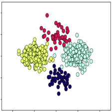
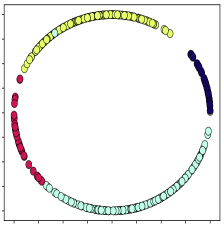
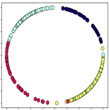
Figure 1: Comparison of Geometric Harmonization and the plain SSL method on a 2-D imbalanced synthetic dataset. (Left) Visualization of the 2-D synthetic dataset. (Middle) The embedding distribution of each category learnt by the vanilla contrastive learning loss is approximately proportional to the number of samples, leading to the undesired representation learning disparity. (Right) GH mitigates the adverse effect of class imbalance and approaches to the category-level uniformity.

We rethink the characteristic of the contrastive learning loss, and try to understand “Why the conventional contrastive learning underperforms in self-supervised long-tailed context?” To answer this question, let us consider two types of representation uniformity: (1) Sample-level uniformity. As stated in [62], the contrastive learning targets to distribute the representation of data points uniformly in the embedding space. Then, the feature span of each category is proportional to their corresponding number of samples. (2) Category-level uniformity. This uniformity pursues to split the region equally for different categories without considering their corresponding number of samples [49, 19]. In the class-balanced scenarios, the former uniformity naturally implies the latter uniformity, resulting in the equivalent separability for classification. However, in the long-tailed distributions, they are different: sample-level uniformity leads to the feature regime that is biased towards the head classes considering their dominant sample quantity and sacrifices the tail classes due to the limited sample quantity. By contrast, category-level uniformity means the equal allocation w.r.t. classes, which balances the space of head and tail classes, and is thus more benign to the downstream classification [17, 19, 37]. Unfortunately, there is no support for promoting category-level uniformity in contrastive learning loss, which explains the question arisen at the beginning.

In this study, we propose a novel method, termed as Geometric Harmonization (GH) to combat representation learning disparity in SSL under long-tailed distributions. Specially, GH uses a geometric uniform structure to measure the uniformity of the embedding space in the coarse granularity. Then, a surrogate label allocation is computed to provide a fine-grained instance-wise calibration, which explicitly compresses the greedy representation space expansion of head classes, and constrain the passive representation space collapse of tail classes. The alternation in the conventional loss refers to an extra efficient optimal-transport optimization that dynamically pursues the category-level uniformity. In Figure 1, we give a toy experiment to visualize the distribution of the embedding space without and with GH. In a nutshell, our contributions can be summarized as follows,

1. To our best knowledge, we are the first to investigate the drawback of the contrastive learning loss in self-supervised long-tailed context and point out that the resulted sample-level uniformity is an intrinsic limitation to the representation parity, motivating us to pursue category-level uniformity with more benign downstream generalization (Section 3.2).

2. We develop a novel and efficient Geometric Harmonization (Figure 2) to combat the representation learning disparity in SSL, which dynamically harmonizes the embedding space of SSL to approach the category-level uniformity with the theoretical guarantee.

3. Our method can be easily plugged into existing SSL methods for addressing the data imbalance without much extra cost. Extensive experiments on a range of benchmark datasets demonstrate the consistent improvements in learning robust representation with our GH.

2 Related Work

Self-Supervised Long-tailed Learning. There are several recent explorations devoted to this direction [40, 28, 59, 41, 77]. BCL [77] leverages the memorization effect of DNNs to automatically drive an instance-wise augmentation, which enhances the learning of tail samples. SDCLR [28] constructs a self-contrast between model and its pruned counterpart to learn more balanced representation. Classic Focal loss [40] leverages the loss statistics to putting more emphasis on the hard examples, which has been applied to self-supervised long-tailed learning [77]. DnC [59] benefits from the parameter isolation of multi-experts during the divide step and the information aggregation during the conquer step to prevent the dominant invasion of majority. Liu et al. [41] proposes to penalize the sharpness surface in a reweighting manner to calibrate class-imbalance learning. Recently, TS [35] employs a dynamic strategy on the temperature factor of contrastive loss, harmonizing instance discrimination and group-wise discrimination. PMSN [2] proposes the power-law distribution prior, replacing the uniform prior, to enhance the quality of learned representations.

Hyperspherical Uniformity. The distribution uniformity has been extensively explored from the physic area, e.g., Thomson problem [58, 53], to machine learning area like some kernel-based extensions, e.g., Riesz s-potential [21, 43] or Gaussian potential [12, 4, 62]. Some recent explorations regarding the features of DNNs [49, 17, 47] discover a terminal training stage when the embedding collapses to the geometric means of the classifier w.r.t. each category. Specially, these optimal class means specify a perfect geometric uniform structure with clear geometric interpretations and generalization guarantees [78, 67, 31]. In this paper, we first extend this intuition into self-supervised learning and leverage the specific structure to combat the representation disparity in SSL.

3 Method

3.1 Problem Formulation

We denote the dataset $\mathcal{D}$, for each data point $({\bm{x}},{\bm{y}})\in\mathcal{D}$, the input ${\bm{x}}\in\mathbb{R}^{m}$ and the associated label ${\bm{y}}\in\{1,\dots,L\}$. Let $N$ denote the number of samples, $\mathrm{R}={N_{max}}/{N_{min}}$ denote the imbalanced ratio (IR), where $N_{max},N_{min}$ is the number of samples in the largest and smallest class, respectively. Let $n_{i}$ denote the number of samples in class $i$. In SSL, the ground-truth ${\bm{y}}$ can not be accessed and the goal is to transform an image to an embedding via DNNs, i.e., $f_{\theta}:\mathbb{R}^{m}\rightarrow\mathbb{R}^{d}$. In the linear probing evaluation, we construct a supervised learning task with balanced datasets. A linear classifier $g(\cdot)$ is built on top of the frozen $f_{\theta}(\cdot)$ to produce the prediction, i.e., $g(f_{\theta}({\bm{x}}))$.

3.2 Geometric Harmonization

As aforementioned, most existing SSL methods in long-tailed context leverage the contrastive learning loss, which encourages the sample-level uniformity in the embedding space. Considering the intrinsic limitation illustrated in Figure 1, we incorporate the geometric clues from the embedding space to calibrate the current loss, enabling our pursuit of category-level uniformity. In the following, we first introduce a specific geometric structure that is critical to Geometric Harmonization.

Definition 3.1.

(Geometric Uniform Structure). Given a set of vertices $\mathbf{M}\in\mathbb{R}^{d\times K}$, the geometric uniform structure satisfies the following between-class duality

$$\mathbf{M}_{i}^{\top}\cdot\mathbf{M}_{j}=C,\ \ \forall i,j\in\{1,2,\ldots,K\},\ i\neq j,$$ (1)

where $\left\lVert\mathbf{M}_{i}\right\rVert=1,\forall i\in\{1,2,\ldots,K\}$, $K$ is the number of geometric vertices and $C$ is a constant.

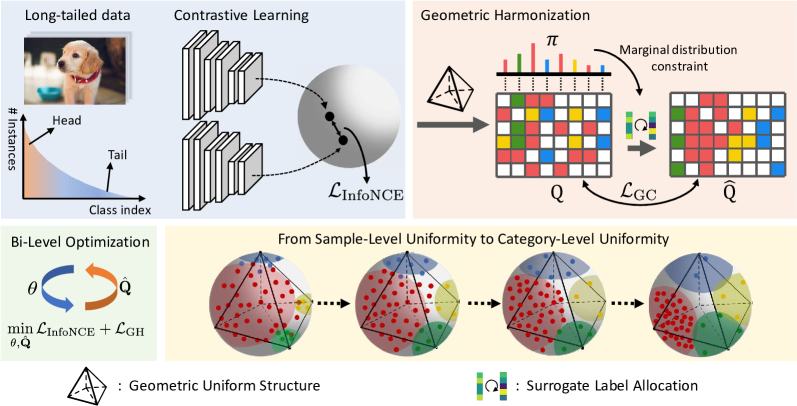
Figure 2: Overview of Geometric Harmonization (w/ InfoNCE). To achieve harmonization with the category-level uniformity, we require ground-truth labels for supervision during training. However, these labels are not available under the self-supervised paradigm. Moreover, estimating surrogate labels directly from the geometric uniform structure is challenging and noisy, especially when the representation is not ideally distributed. To fullfill this gap, we utilize the geometric uniform structure to measure the embedding space, and the captured population statistics are used for an instance-wise calibration by surrogate label allocation, which provides a supervision feedback to counteract the sample-level uniformity. Specially, our method are theoretically grounded to approach category-level uniformity at the loss minimum. The additional model parameters incurred by GH are analytically and empirically demonstrated to be trained in an efficient manner.

Above structure provides a characteristic that any two vectors in $\mathbf{M}$ have the same angle, namely, the unit space are equally partitioned by the vectors in $\mathbf{M}$. This fortunately follows our expectation about category-level uniformity. Specially, if we use $\mathbf{M}$ as a constant classifier to involve into training, and have the oracle label ${\bm{y}}$ of the long-tailed data ($K=L$) to supervise the below prediction

$${\bm{q}}=p({\bm{y}}|f_{\theta}({\bm{x}}),\mathbf{M})=\exp\left(\mathbf{M}_{y}^{\top}\cdot f_{\theta}({\bm{x}})/\gamma_{\mathrm{GH}}\right)\big{/}\left(\sum_{i=1}^{K}\exp\left(\mathbf{M}_{i}^{\top}\cdot f_{\theta}({\bm{x}})/\gamma_{\mathrm{GH}}\right)\right),$$ (2)

then according to the neural collapse theory [49], the representation of all samples will fit the geometric uniform structure of $\mathbf{M}$ in the limit, namely, approach category-level uniformity. However, the technical challenge is the complete absence of annotation ${\bm{y}}$ in our context, making directly constructing the objective $\min\mathbb{E}[{\bm{y}}\log{\bm{q}}]$ with Eq. (2) impossible to combat the representation disparity.

Surrogate Label Allocation. To address the problem of unavailable labels, we explore constructing the surrogate geometric labels $\hat{{\bm{q}}}$ to supervise the training of Eq. (2). Concretely, we utilize the recent discriminative clustering idea [1] to acquire such geometric labels, formulated as follows

$$\min_{\hat{\mathbf{Q}}=[\hat{{\bm{q}}}_{1},\dots,\hat{{\bm{q}}}_{N}]}\mathcal{L}_{\mathrm{GH}}=-\frac{1}{|\mathcal{D}|}\sum_{{\bm{x}}_{i}\sim\mathcal{D}}\hat{{\bm{q}}_{i}}\log{\bm{q}}_{i},\ \ \ \mathrm{s.t.}\ \ \hat{\mathbf{Q}}\cdot\mathbbm{1}_{N}=N\cdot\bm{\pi},\ \hat{\mathbf{Q}}^{\top}\cdot\mathbbm{1}_{K}=\mathbbm{1}_{N},$$ (3)

where $\hat{{\bm{q}}}_{i}$ refers to the soft assignment constrained in a $K$-dimensional probability simplex and $\bm{\pi}\in\mathbb{R}^{K}_{+}$ refers to the distribution constraint. As we are dealing with long-tailed data, we propose to use the geometric uniform structure $\bm{\mathbf{M}}$ to automatically compute the population statistic of the embedding space as $\bm{\pi}$. Finally, Eq. (3) can be analytically solved by Sinkhorn-Knopp algorithm [14] (refer to Appendix D for Algorithm 1). Note that, the above idea builds upon a conjecture: the constructed surrogate geometric labels are mutually correlated with the oracle labels so that they have the similar implication to approach category-level uniformity. We will empirically verify the rationality of such an assumption via normalized mutual information in Section 4.4.

Overall Objective. Eq. (3) can be easily integrated into previous self-supervised long-tailed learning methods for geometric harmonization, e.g., SDCLR [28] and BCL [77]. For simplicity, we take their conventional InfoNCE loss [48] as an example and write the overall objective as follows

$$\min_{\theta,\hat{\mathbf{Q}}}\mathcal{L}=\mathcal{L}_{\mathrm{InfoNCE}}+w_{\mathrm{GH}}\mathcal{L}_{\mathrm{GH}},$$ (4)

where $w_{\mathrm{GH}}$ represents the weight of the geometric harmonization loss. Optimizing Eq. (4) refers to a bi-level optimization style: in the outer-loop, optimize $\min_{\hat{\mathbf{Q}}}\mathcal{L}_{\mathrm{GH}}$ with fixing $\theta$ to compute the surrogate geometric labels; in the inner-loop, optimize $\min_{\theta}\mathcal{L}_{\mathrm{InfoNCE}}+\mathcal{L}_{\mathrm{GH}}$ with fixing $\hat{\mathbf{Q}}$ to learn the representation model. The additional cost compared to the vanilla method primarily arises from from the outer-loop, which will be discussed in Section 3.4 and verified in Section 4.4.

Table 1: Linear probing of vanilla discriminative clustering methods and variants of GH on CIFAR-100-LT.

IR	SimCLR	+SeLA	+SwAV	+GH	w/o GUS	w/o $\bm{\pi}$
100	50.7	50.5	52.2	54.0	53.3	53.1
50	52.2	52.0	53.0	55.4	54.6	54.4
10	55.7	56.0	56.1	57.4	56.7	56.4

Compared with previous explorations [1, 7], the uniqueness of GH lies in the following three aspects: (1) Geometric Uniform Structure. The pioneering works mainly resort to a learnable classifier to perform clustering, which can easily be distorted in the long-tailed scenarios [17]. Built on the geometric uniform classifier, our method is capable to provide high-quality clustering results with clear geometric interpretations. (2) Flexible Class Prior. The class prior $\bm{\pi}$ is assumed to be uniform among the previous attempts. When moving to the long-tailed case, this assumption will strengthen the undesired sample-level uniformity. In contrast, our methods can potentially cope with any distribution with the automatic surrogate label allocation. (3) Theoretical Guarantee. GH is theoretically grounded to achieve the category-level uniformity in the long-tailed scenarios (refer to Section 3.3), which has never been studied in previous methods. To gain more insights into our method, we further compare GH with discriminative clustering methods (SeLA [1], SwAV [7]) and investigate the impact of various components in GH. From the results in Table 1, we can see that GH consistently outperforms the vanilla discriminative clustering baselines in the linear probing evaluation. Notably, we observe that both GUS and the class prior $\bm{\pi}$ play a critical role in our GH.

3.3 Theoretical Understanding

Here, we reveal the theoretical analysis of GH on promoting the representation learning to achieve category-level uniformity instead of sample-level uniformity. Let us begin with a deteriorated case of sample-level uniformity under the extreme imbalance, i.e., minority collapse [17].

Lemma 3.2.

(Minority collapse) Assume the samples follow the uniform distribution $n_{1}=n_{2}=\dots=n_{L_{H}}=n_{H}$, $n_{L_{H}+1}=n_{L_{H}+2}=\dots=n_{L}=n_{T}$ in head and tail classes respectively. Assume $d\geq L$ and $n_{H}/n_{T}\rightarrow+\infty$, the lower bound (Lemma C.1) of $\mathcal{L}_{\mathrm{InfoNCE}}$ achieves the minimum when the class means of the tail classes collapse to an identical vector:

$$\lim\bm{\mu}_{i}-\bm{\mu}_{j}=\mathbf{0}_{L},\ \forall L_{H}\leq i\leq j\leq L,$$

where $\bm{\mu}_{l}=\frac{1}{n_{l}}\sum_{i=1}^{n_{l}}f_{\theta}({\bm{x}}_{l,i})$ denotes the class means and ${\bm{x}}_{l,i}$ is the $i$-th data point with label $l$.

This phenomenon indicates all representations of the minority will collapse completely to one point without considering the category discrepancy, which aligns with our observation regarding the passive collapse of tailed samples in Figure 1. To further theoretically analyze GH, we first quantitatively define category-level uniformity in the following, and then theoretically claim that with the geometric uniform structure (Definition. 3.1) and the perfect aligned allocation (Eq. (3)), we can achieve the loss minimum at the stage of realizing category-level uniformity.

Definition 3.3.

(Categorical-level Uniformity) We define categorical-level uniformity on the embedding space w.r.t the geometric uniform structure $\mathbf{M}$ when it satisfies

$$\bm{\mu}_{k}^{*}=\mathbf{M}_{k},\ \forall k=1,2,\dots,K,$$

where $\bm{\mu}_{k}^{*}=\frac{1}{n_{k}}\sum_{i=1}^{n_{k}}f_{\theta}^{*}({\bm{x}}_{k,i})$ represents the class mean for samples assigned with the surrogate geometric label $k$ in the embedding space.

Theorem 3.4.

(Optimal state for $\mathcal{L}$) Given Eq. (4) under the proper optimization strategy, when it arrives at the category-level uniformity (Definition 3.3) defined on the geometric uniform structure $\mathbf{M}$ (Definition 3.1), we will achieve the minimum of the overall loss $\mathcal{L}^{*}$ as

$$\mathcal{L}^{*}=-2\sum_{l=1}^{L}\bm{\pi}_{l}^{{\bm{y}}}\log\left(1/\left(1+(K-1)\exp(C-1)\right)\right)+\log\left(J/L\right),$$ (5)

where $J$ denotes the size of the collection of the negative samples and $\bm{\pi}^{{\bm{y}}}$ refers to the marginal distribution of the latent ground-truth labels ${\bm{y}}$.

This guarantees the desirable solution with the minimal intra-class covariance and the maximal inter-class covariance under the geometric uniform structure [49, 17], which benefits the downstream generalization. Notably, no matter the data distribution is balanced or not, our method can persistently maintain the theoretical merits on calibrating the class means to achieve category-level uniformity. We also empirically demonstrate the comparable performance with GH on the balanced datasets in Section 4.4, as in this case category-level uniformity is equivalent to sample-level uniformity.

3.4 Implementation and Complexity analysis

In Algorithm 2 of Appendix D, we give the complete implementation of our method. One point that needs to be clarified is that we learn the label allocation $\hat{{\bm{q}}}$ in the mini-batch manner. In addition, the geometric prediction ${\bm{q}}$ and the adjusted $\hat{{\bm{q}}}$ are computed at the beginning of every epoch as the population-level statistic will not change much in a few mini-batches. Besides, we maintain a momentum update mechanism to track the prediction of each sample to stabilize the training, i.e., ${\bm{q}}^{m}\leftarrow\beta{\bm{q}}^{m}+(1-\beta){\bm{q}}$. When combined with the joint-embedding loss, we naturally adopt a cross-supervision mechanism $\min\mathbb{E}[\hat{{\bm{q}}}^{+}\log{\bm{q}}]$ for the reconciliation with contrastive baselines. The proposed method is illustrated in Figure 2 for visualization.

For complexity, assume that the standard optimization of deep neural networks requires forward and backward step in each mini-batch update with the time complexity as $\mathcal{O}(B\Lambda)$, where $B$ is the mini-batch size and $\Lambda$ is the parameter size. At the parameter level, we add an geometric uniform structure with the complexity as $\mathcal{O}(BKd)$, where $K$ is the number of geometric labels and $d$ is the embedding dimension. For Sinkhorn-Knopp algorithm, it only refers to a simple matrix-vector multiplication as shown in Algorithm 1, whose complexity is $\mathcal{O}(E_{s}(B+K+BK))$ with the iteration step $E_{s}$. The complexity incurred in the momentum update is $\mathcal{O}(BK)$. Since $K,d$ and $E_{s}$ are significantly smaller than the model parameter $\Lambda$ of a million scale, the computational overhead involved in GH is negligible compared to $\mathcal{O}(B\Lambda)$. The additional storage for a mini-batch of samples is the matrix $\mathbf{Q}^{m}\in\mathbb{R}^{K\times B}$, which is also negligible to the total memory usage. To the end, GH incurs only a small computation or memory cost and thus can be plugged to previous methods in a low-cost manner. The empirical comparison about the computational cost is summarized in Table 17.

4 Experiments

4.1 Experimental Setup

Baselines. We mainly choose five baseline methods, including (1) plain contrastive learning: SimCLR [9], (2) hard example mining: Focal [40], (3) asymmetric network pruning: SDCLR [28], (4) multi-expert ensembling: DnC [59], (5) memorization-guided augmentation: BCL [77]. Empirical comparisons with more baseline methods can be referred to Section F.3.

Implementation Details. Following previous works [28, 77], we use ResNet-18 [23] as the backbone for small-scale dataset (CIFAR-100-LT [5]) and ResNet-50 [23] for large-scale datasets (ImageNet-LT [44], Places-LT [44]). For experiments on CIFAR-100-LT, we train model with the SGD optimizer, batch size 512, momentum 0.9 and weight decay factor $5\times 10^{-4}$ for 1000 epochs. For experiments on ImageNet-LT and Places-LT, we only train for 500 epochs with the batch size 256 and weight decay factor $1\times 10^{-4}$. For learning rate schedule, we use the cosine annealing decay with the learning rate $0.5\rightarrow 1e^{-6}$ for all the baseline methods. As GH is combined with baselines, a proper warming-up of 500 epochs on CIFAR-100-LT and 400 epochs on ImageNet-LT and Places-LT are applied. The cosine decay is set as $0.5\rightarrow 0.3$, $0.3\rightarrow 1e^{-6}$ respectively. For hyper-parameters of GH, we provide a default setup across all the experiments: set the geometric dimension $K$ as 100, $w_{\mathrm{GH}}$ as 1 and the temperature $\gamma_{\mathrm{GH}}$ as 0.1. In the surrogate label allocation, we set the regularization coefficient $\lambda$ as 20 and Sinkhorn iterations $E_{s}$ as 300. Please refer to Section E.3 for more experimental details.

Evaluation Metrics. Following [28, 77], linear probing on a balanced dataset is used for evaluation. We conduct full-shot evaluation on CIFAR-100-LT and few-shot evaluation on ImageNet-LT and Places-LT. For comprehensive performance comparison, we present the linear probing performance and the standard deviation among three disjoint groups, i.e., [many, medium, few] partitions [44].

4.2 Linear Probing Evaluation

Table 2: Linear probing results on CIFAR-100-LT with different imbalanced ratios (100, 50, 10), ImageNet-LT and Places-LT. Many/Med/Few ($\uparrow$) indicate the average accuracy ($\%$) w.r.t fine-grained partitions according to the class cardinality. Std ($\downarrow$) means the standard deviation of the group-level performance and Avg ($\uparrow$) is the average accuracy ($\%$) of the full test set. Following the previous work [28, 77], Std represents a balancedness measure to quatify the variance among three specified groups. Improv. ($\uparrow$) represents the averaging performance improvements w.r.t. different baseline methods. We report the error bars with the multi-run experiments in Table 12 in Appendix F.

Dataset		SimCLR	+GH	Focal	+GH	SDCLR	+GH	DnC	+GH	BCL	+GH	Improv.
CIFAR-R100	Many	54.97	57.38	54.24	57.01	57.32	57.44	55.41	57.56	59.15	59.50	+1.56
	Med	49.39	52.27	49.58	52.93	50.70	52.85	51.30	53.74	54.82	55.73	+2.35
	Few	47.67	52.12	49.21	51.74	50.45	54.06	50.76	53.26	55.30	57.67	+3.09
	Std	3.82	2.99	2.80	2.76	3.90	2.38	2.54	2.36	2.37	1.89	-0.61
	Avg	50.72	53.96	51.04	53.92	52.87	54.81	52.52	54.88	56.45	57.65	+2.32
CIFAR-R50	Many	56.00	58.88	55.40	57.97	57.50	58.47	56.03	59.04	59.44	60.82	+2.16
	Med	50.48	53.00	51.14	53.55	51.85	53.88	52.68	55.05	54.73	57.58	+2.44
	Few	50.12	54.27	50.02	53.58	52.15	53.58	50.83	54.81	57.30	58.55	+2.87
	Std	3.30	3.09	2.84	2.54	3.18	2.74	2.64	2.38	2.36	1.66	-0.38
	Avg	52.24	55.42	52.22	55.06	53.87	55.34	53.21	56.33	57.18	59.00	+2.49
CIFAR-R10	Many	57.85	59.26	58.18	60.06	58.47	59.21	59.82	61.09	60.41	61.41	+1.26
	Med	55.06	56.91	55.82	56.79	54.79	56.06	56.67	58.33	57.15	59.27	+1.57
	Few	54.03	55.85	54.64	57.24	52.97	55.58	56.21	57.33	59.76	60.30	+1.74
	Std	1.98	1.75	1.80	1.77	2.80	1.97	1.96	1.95	1.73	1.07	-0.35
	Avg	55.67	57.36	56.23	58.05	55.44	56.97	57.59	58.94	59.12	60.34	+1.52
ImageNet-LT	Many	41.69	41.53	42.04	42.55	40.87	41.92	41.70	42.19	42.92	43.22	+0.44
	Med	33.96	36.35	35.02	36.75	33.71	36.53	34.68	36.63	35.89	38.16	+2.23
	Few	31.82	35.84	33.32	36.28	32.07	36.04	33.58	35.86	33.93	36.96	+3.25
	Std	5.19	3.15	4.62	3.49	4.68	3.26	4.41	3.45	4.73	3.32	-1.39
	Avg	36.65	38.28	37.49	38.92	36.25	38.53	37.23	38.67	38.33	39.95	+1.68
Places-LT	Many	31.98	32.46	31.69	32.40	32.17	32.78	32.07	32.51	32.69	33.22	+0.55
	Med	34.05	35.03	34.33	35.14	34.71	35.60	34.51	35.55	35.37	36.00	+0.87
	Few	35.63	36.14	35.73	36.49	35.69	36.18	35.84	35.91	37.18	37.62	+0.45
	Std	1.83	1.89	2.05	2.08	1.82	1.82	1.91	1.87	2.26	2.23	0.00
	Avg	33.61	34.33	33.65	34.42	33.99	34.70	33.90	34.52	34.76	35.32	+0.68

CIFAR-100-LT. In Table 2, we summarize the linear probing performance of baseline methods w/ and w/o GH on a range of benchmark datasets, and provide the analysis as follows.

(1) Overall Performance. GH achieves the competitive results w.r.t the [many, medium, few] groups, yielding a overall performance improvements averaging as 2.32$\%$, 2.49$\%$ and 1.52$\%$ on CIFAR-100-LT with different imbalanced ratios. It is worth noting that on the basis of the previous state-of-the-art BCL, our GH further achieves improvements by 1.20$\%$, 1.82$\%$ and 1.22$\%$, respectively. Our GH consistently improves performance across datasets with varying degrees of class imbalance, demonstrating its potential to generalize to practical scenarios with more complex distributions. Specially, our method does not require any prior knowledge or assumptions about the underlying data distribution, highlighting the robustness and versatility to automatically adapt to the data.

(2) Representation Balancedness. In Section 1, we claim that GH helps compress the expansion of head classes and avoid the passive collapse of tail classes, yielding the more balanced representation distribution. To justify this aspect, we compare the variance in linear probing performance among many/medium/few groups, namely, their groupwise standard deviation. According to Table 2, our GH provides [1.56$\%$, 2.35$\%$, 3.09$\%$], [2.16$\%$, 2.44$\%$, 2.87$\%$] and [1.26$\%$, 1.57$\%$, 1.74$\%$] improvements w.r.t [many, medium, few] groups on CIFAR-100-LT-R100/R50/R10 with more preference to the minority classes for representation balancedness. Overall, GH substantially improves the standard deviation by [0.61, 0.38, 0.35] on different levels of imbalance.

ImageNet-LT and Places-LT. Table 2 shows the comparison of different baseline methods on large-scale dataset ImageNet-LT and Places-LT, in which we have consistent observations. As can be seen, on more challenging real-world dataset, GH still outperforms other methods in terms of overall accuracy, averaging as 1.68$\%$, 0.68$\%$ on ImageNet-LT and Places-LT. Specifically, our method provides [0.44$\%$, 2.23$\%$, 3.25$\%$] and [0.55$\%$, 0.87$\%$, 0.45$\%$] improvements in linear probing w.r.t. [many, medium, few] groups on ImageNet-LT and Places-LT. The consistent performance overhead indicates the robustness of our method to deal with long-tailed distribution with different characteristics. Moreover, the averaging improvement of standard deviation is 1.39 on ImageNet-LT, indicating the comprehensive merits of our GH on the minority classes towards the representation balancedness. However, an interesting phenomenon is that the fine-grained performance exhibits a different trend on Places-LT. As can be seen, the performance of head classes is even worse than that of tail classes. The lower performance of the head partition can be attributed to the fact that it contains more challenging classes. As a result, we observe that the standard deviation of our GH does not significantly decrease on Places-LT, which requires more effort and exploration for improvement alongside GH.

Table 3: Supervised long-tailed learning by finetuning on CIFAR-100-LT, ImageNet-LT and Places-LT. We compare the performance of five self-supervised learning methods as the pre-training stage for downstream supervised logit adjustment [46] method. Improv. ($\uparrow$) represents the averaging performance improvements w.r.t. different baseline methods. Besides, the performance of logit adjustment via learning from scratch is also reported for comparisons.

Dataset	LA	Logit adjustment pretrained with the following SSL methods										Improv.
		SimCLR	+GH	Focal	+GH	SDCLR	+GH	DnC	+GH	BCL	+GH
CIFAR-LT	46.61	49.81	50.84	49.83	51.04	49.79	50.73	49.97	50.84	50.38	51.32	+1.00
ImageNet-LT	48.27	51.10	51.67	51.15	51.82	50.94	51.64	51.31	51.88	51.43	52.06	+0.63
Places-LT	27.07	32.63	33.86	32.69	33.75	32.55	34.03	32.98	34.09	33.15	34.48	+1.24

4.3 Downstream Finetuning Evaluation

Downstream supervised long-tailed learning. Self-supervised learning has been proved to be beneficial as a pre-training stage of supervised long-tailed recognition to exclude the explicit bias from the class imbalance [68, 41, 77].

To validate the effectiveness of our GH, we conduct self-supervised pre-training as the initialization for downstream supervised classification tasks on CIFAR-100-LT-R100, ImageNet-LT and Places-LT. The state-of-the-art logit adjustment [46] is chosen as the downstream baseline. The combination of GH + LA can be interpreted as a compounded method where GH aims at the re-balanced representation extraction and LA targets the classifier debiasing. In Table 3, we can find that the superior performance improvements are achieved by self-supervised pre-training over the plain supervised learning baseline. Besides, our method can also consistently outperform other SSL baselines, averaging as 1.00$\%$, 0.63$\%$ and 1.24$\%$ on CIFAR-100-LT-R100, ImageNet-LT and Places-LT. These results demonstrate that GH are well designed to facilitate long-tailed representation learning and improve the generalization for downstream supervised tasks.

Cross-dataset transfer learning. To further demonstrate the representation transferability of our GH, we conduct more comprehensive experiments on the large-scale, long-tailed dataset CC3M [52] with various cross-dataset transferring tasks, including downstream classification, object detection and instance segmentation. Specifically, we report the finetuning classification performance on ImageNet, Places and fine-grained visual datasets Caltech-UCSD Birds (CUB200) [61], Aircrafts [45], Stanford Cars [33], Stanford Dogs [32], NABirds [60]. Besides, we evaluate the quality of the learned representation by finetuning the model for object detection and instance segmentation on COCO2017 benchmark [39]. As shown in Tables 4 and 6, we can see that our proposed GH consistently outperforms the baseline across various tasks and datasets. It further demonstrates the importance of considering long-tailed data distribution under large-scale unlabeled data in the pretraining stage. This can potentially be attributed to that our geometric harmonization motivates a more balanced and general emebdding space, improving the generalization ability of the pretrained model to a range of real-world downstream tasks.

Table 4: Image classification on ImageNet, Places and fine-grained visual classification on various fine-grained datasets, pretrained on large-scale long-tailed CC3M and then finetuned.

	Image Classification			Fine-Grained Visual Classification
	ImageNet	Places		CUB200	Aircraft	StanfordCars	StanfordDogs	NABirds	Average
SimCLR	52.06	37.65		44.61	65.89	57.63	50.99	46.86	53.20
+GH	53.39	38.47		45.76	68.08	60.24	52.88	47.58	54.91

Table 5: Object detection and instance segmentation with finetuned features on COCO2017 benchmark, pretrained on large-scale long-tailed CC3M.

	Object Detection				Instance Segmentation
	APbbox	AP${}^{bbox}_{50}$	AP${}^{bbox}_{75}$		APmask	AP${}^{mask}_{50}$	AP${}^{mask}_{75}$
SimCLR	31.7	51.0	33.9		30.2	49.8	32.1
+GH	32.7	52.2	35.2		31.1	50.8	33.0

Table 6: Inter-class uniformity ($\uparrow$) and neighborhood uniformity ($\uparrow$) of pretrained features on CIFAR-LT.

	Inter-class Uniformity			Neighborhood Uniformity
	SimCLR	+GH		SimCLR	+GH
C100	1.00	2.80		0.72	2.00
C50	1.23	2.73		0.91	1.94
C10	1.18	2.60		0.85	1.83

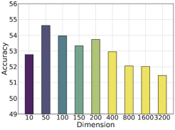
(a) Geometric Dimension

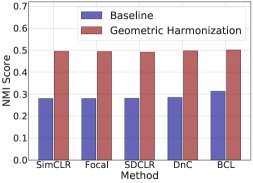
(b) Label Quality

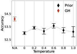
(c) Label-Distribution Prior

Figure 3: (a) Linear probing performance w.r.t. the dimension $K$ of the geometric uniform structure $\mathbf{M}$ (Appendix B) on CIFAR-LT-R100. (b) NMI score between the surrogate geometric labels and the ground-truth labels in the training stage on CIFAR-LT-R100. (c) Average linear probing and the error bars of the surrogate label allocation with variants of the label prior on CIFAR-LT-R100.

Table 7: Linear probing of more SSL variants on CIFAR-100-LT with different imbalanced ratios.

Dataset	SimSiam	+GH	Barlow	+GH	BYOL	+GH	MoCo-v2	+GH	MoCo-v3	+GH
CIFAR-R100	49.01	51.43	48.70	51.23	51.43	52.87	51.49	53.53	54.08	55.82
CIFAR-R50	48.98	53.54	49.29	51.95	52.04	53.84	52.68	55.01	55.34	56.45
CIFAR-R10	55.51	57.03	53.11	56.34	55.86	57.28	58.23	60.11	59.10	60.57

4.4 Further Analysis and Ablation Studies

Dimension of Geometric Uniform Structure. As there is even no category number $L$ available in SSL paradigm, we empirically compare our GH with different geometric dimension $K$ on CIFAR-100-LT-R100, as shown in Figure 3(a). From the results, GH is generally robust to the change of $K$, but slightly exhibits the performance degeneration when the dimension is extremely large or small. Intuitively, when $K$ is extremely large, our GH might pay more attention to the uniformity among sub-classes, while the desired uniformity on classes is not well guaranteed. Conversely, when $K$ is extremely small, the calibration induced by GH is too coarse that cannot sufficiently avoid the internal collapse within each super-class. For discussions of the structure, it can refer to Appendix B.

Surrogate Label Quality Uncovered. To justify the effectiveness of surrogate label allocation, we compare the NMI scores [54] between the surrogate and ground-truth label in Figure 3(b). We observe that GH significantly improves the NMI scores across baselines, indicating that the geometric labels are effectively calibrated to better capture the latent semantic information. Notably, the improvements of the existing works are marginal, which further verifies the superiority of GH.

Exploration with Other Label-Distribution Prior. To further understand $\bm{\pi}$, we assume the ground-truth label distribution is available and incorporate the oracle $\bm{\pi}^{{\bm{y}}}$ into the surrogate label allocation. Comparing the results of the softened variants $\bm{\pi}_{\gamma_{\mathrm{T}}}^{{\bm{y}}}$ with the temperature ${\gamma_{\mathrm{T}}}$ in Figure 3(c), we observe that GH outperforms all the counterparts equipped with the oracle prior. A possible reason is that our method automatically captures the inherent geometric statistics from the embedding space, which is more reconcilable to the self-supervised learning objectives.

Uniformity Analysis. In this part, we conduct experiments with two uniformity metrics [62, 37]:

$$\mathrm{U}=\frac{1}{L(L-1)}\sum_{i=1}^{L}\sum_{j=1,j\neq i}^{L}||\bm{\mu}_{i}-\bm{\mu}_{j}||_{2},\ \ \ \mathrm{U}_{k}=\frac{1}{Lk}\sum_{i=1}^{L}\min_{j_{1},\dots,j_{k}}(\sum_{m=1}^{k}||\bm{\mu}_{i}-\bm{\mu}_{j_{m}}||_{2}),$$

where $j_{1},\dots,j_{k}\neq i$ represent different classes. Specifically, $\mathrm{U}$ evaluates average distances between different class centers and $\mathrm{U}_{k}$ measures how close one class is to its neighbors. As shown in Table 6, our GH outperforms in both inter-class uniformity and neighborhood uniformity when compared with the baseline SimCLR [9]. This indicates that vanilla contrastive learning struggles to achieve the uniform partitioning of the embedding space, while our GH effectively mitigates this issue.

Comparison with More SSL Methods. In Table 7, we present a more comprehensive comparison of different SSL baseline methods, including MoCo-v2 [24], MoCo-v3 [11] and various non-contrastive methods such as SimSiam [10], BYOL [20] and Barlow Twins [71]. From the results, we can see that the combinations of different SSL methods and our GH can achieve consistent performance improvements, averaging as 2.33$\%$, 3.18$\%$ and 2.21$\%$ on CIFAR-100-LT. This demonstrates the prevalence of representation learning disparity under data imbalance in general SSL settings.

Table 8: Linear probing of joint optimization on CIFAR-100-LT with different IRs.

Method	C100	C50	C10
SimCLR	50.72	52.24	55.67
+GH (Joint)	50.18	52.31	54.98
w/ warm-up	51.14	52.75	55.37
+GH (Bi-level)	53.96	55.42	57.36

On Importance of Bi-Level Optimization. In Table 8, we empirically compare the direct joint optimization strategy to Eq. (4). From the results, we can see that the joint optimization (w/ or w/o the warm-up strategy) does not bring significant performance improvement over SimCLR compared with that of our bi-level optimization, probably due to the undesired collapse in label allocation [1]. This demonstrates the necessity of the proposed bi-level optimization for Eq. (4) to stabilize the training.

Qualitative Visualization. We conduct t-SNE visualization of the learned features to provide further qualitative intuitions. For simplity, we randomly selected four head classes and four tail classes on CIFAR-LT to generate the t-SNE plots. Based on the results in Figure 5, the observations are as follows: (1) SimCLR: head classes exhibit a large presence in the embedding space and heavily squeeze the tail classes, (2) GH: head classes reduce their occupancy, allowing the tail classes to have more space. This further indicates that the constructed surrogate labels can serve as the high-quality supervision, effectively guiding the harmonization towards the geometric uniform structure.

Sensitivity Analysis. To further validate the stability of our GH, We conduct empirical comparison with different weight $w_{\mathrm{GH}}$, temperature $\gamma_{\mathrm{GH}}$, regularization coefficient $\lambda$ and Sinkhorn iteration $E_{s}$ on CIFAR-LT, as shown in Figures 5 and 7. From the results, we can see that our GH can consistently achieve satisfying performance with different hyper-parameter.

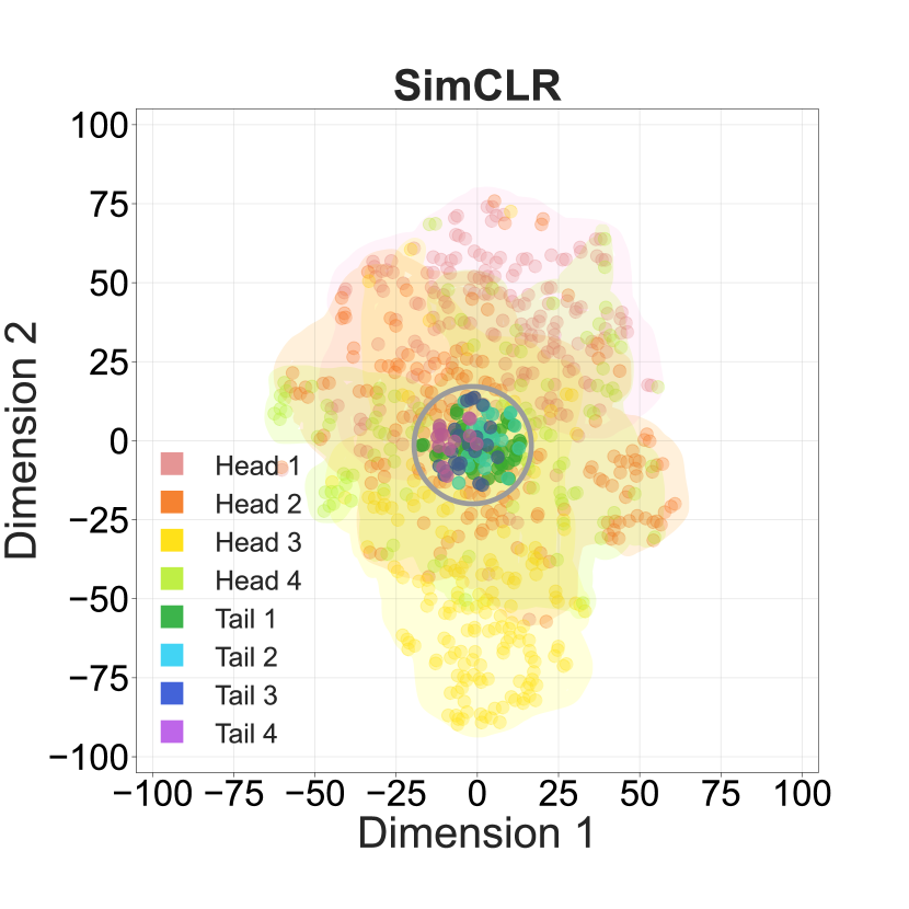
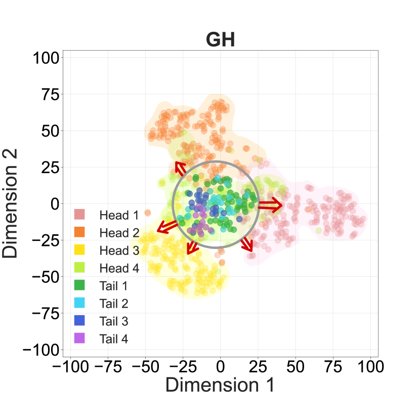
Figure 4: T-SNE visualization of the pretrained features from 8 randomly selected classes w.r.t CIFAR-LT training images.

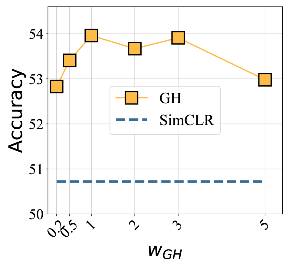
Figure 5: Ablations of $w_{GH}$ on CIFAR-LT.

5 Conclusion

In this paper, we delve into the defects of the conventional contrastive learning in self-supervised long-tail context, i.e., representation learning disparity, motivating our exploration on the inherent intuition for approaching the category-level uniformity. From the geometric perspective, we propose a novel and efficient Geometric Harmonization algorithm to counteract the long-tailed effect on the embedding space, i.e, over expansion of the majority class with the passive collapse of the minority class. Specially, our proposed GH leverages the geometric uniform structure as an optimal indicator and manipulate a fine-grained label allocation to rectify the distorted embedding space. We theoretically show that our proposed method can harmonize the desired geometric property in the limit of loss minimum. It is also worth noting that our method is orthogonal to existing self-supervised long-tailed methods and can be easily plugged into these methods in a lightweight manner. Extensive experiments demonstrate the consistent efficacy and robustness of our proposed GH. We believe that the geometric perspective has the great potential to evolve the general self-supervised learning paradigm, especially when coping with the class-imbalanced scenarios.

Contents

[chapters] [chapters]11em

Reproducibility Statement

We provide our source codes to ensure the reproducibility of our experimental results. Below we summarize several critical aspects w.r.t the reproducible results:

• Datasets. The datasets we used are all publicly accessible, which is introduced in Section E.1. For long-tailed subsets, we strictly follows previous work [29] on CIFAR-100-LT to avoid the bias attribute to the sampling randomness. On ImageNet-LT and Places-LT, we employ the widely-used data split first introduced in [44].

• Source code. Our code is available at https://github.com/MediaBrain-SJTU/Geometric-Harmonization.

• Environment. All the experiments are conducted on NVIDIA GeForce RTX 3090 with Python 3.7 and Pytorch 1.7.

Appendix A Additional Discussions of Related Works

A.1 Supervised Long-tailed Learning

As the explorations on the classifier learning [29, 70] are orthogonal to the self-supervised learning paradigms, we mainly focus on the representation learning in supervised long-tailed recognition. The pioneering work [29] first explores representation and classifier learning with a disentangling mechanisms and shows the merits of instance-balanced sampling strategy on the representation learning stage. Subsequently, Yang and Xu [68] points out the negative impact of label information and proposes to improve the representation learning with semi-supervised learning and self-supervised learning. This motivates a stream of research works diving into the representation learning. Supervised contrastive learning [30, 13] is leveraged with rebalanced sampling or prototypical learning design to pursue a more balanced representation space. Li et al. [37] explicitly regularizes the class centers to a maximum separation structure with similar drives to the balanced feature space.

A.2 Contrastive Learning is Still Vulnerable to Long-tailed Distribution

The prior works [30, 41] point out that contrastive learning can extract more balanced features compared with the supervised learning paradigm. However, several subsequent works [28, 77] empirically observes that contrastive learning is still vulnerable to the long-tailed distribution, which motivates their model-pruning strategy [28] and memorization-oriented augmentation [77] to rebalance the representation learning. In this paper, we delve into the intrinsic limitation of the contrastive learning method in the long-tailed context, i.e, approaching sample-level uniformity to deteriorate the embedding space.

A.3 Unsupervised Clustering

Deep Cluster [6] applies K-Means clustering to generate pseudo-labels for the unlabeled data, which are then iteratively leveraged as the supervised signal to train a classifier. SeLa [1] first casts the pseudo-label generation as an optimal transport problem and leverages a uniform prior to guide the clustering. SwAV [7] adopts mini-batch clustering instead of dataset-level clustering, enhancing the practical applicability of the optimal transport-based clustering method. Subsequently, Li et al. [36] combines clustering and contrastive learning objectives in an Expectation-Maximization framework, recursively updating the data features towards their corresponding class prototypes. In this paper, we propose a novel Geometric Harmonization method that is capable to cope with long-tailed distribution, the uniqueness can be summarized in the following aspects: (1) Geometric Uniform Structure. The pioneering works [1, 7] mainly resort to a learnable classifier to perform clustering, which can easily be distorted in the long-tailed scenarios [17]. Built on the geometric uniform structure, our method is capable to provide high-quality clustering results with clear geometric interpretations. (2) Flexible Class Prior. The class prior in  [1, 7] is assumed to be uniform among the previous attempts. When moving to the long-tailed case, this assumption will strengthen the undesired sample-level uniformity. In contrast, our methods can potentially cope with any distribution with the automatic surrogate label allocation. (3) Theoretical Guarantee. GH is theoretically grounded to achieve the category-level uniformity in the long-tailed scenarios, which has never been studied in previous methods.

A.4 Taxonomy of Self-supervised Long-tailed Methods

We summarize the detailed taxonomy of self-supervised long-tailed methods in Algorithm 1.

Table 9: Taxonomy of self-supervised long-tailed methods.

Method	Aspect	Description
Focal [40]	Sample Reweighting	Hard example mining
rwSAM [41]	Optimization Surface	Data-dependent sharpness-aware minimization
SDCLR [28]	Model Pruning	Model pruning and self-contrast
DnC [59]	Model Capacity	Multi-expert ensemble
BCL [77]	Data Augmentation	Memorization-guided augmentation
GH	Loss Limitation	Geometric harmonization

Appendix B Discussions of Geometric Uniform Structure (Definition 3.1)

B.1 Simplex Equiangular Tight Frame ($K\leq d$)

Neural collapse [47] describes a phenomenon that with the training, the geometric centroid of representation progressively collapses to the optimal classifier parameter w.r.t. each category. The collection of these points builds a special geometric structure, termed as Simplex Equiangular Tight Frame (ETF). Some study that shares the similar spirit is also explored regarding the maximum separation structure [31]. We present its formal definition as follows.

Definition B.1.

A Simplex ETF is a collection of points in $\mathbb{R}^{d}$ specified by the columns of the matrix:

$$\mathbf{M}^{\mathrm{ETF}}=\sqrt{\frac{K}{K-1}}\mathbf{U}(\mathbf{I}_{K}-\frac{1}{K}\mathbbm{1}_{K}\mathbbm{1}^{\mathrm{T}}_{K}),$$ (6)

where $\mathbf{I}_{K}\in\mathbb{R}^{K\times K}$ is the identity matrix and $\mathbbm{1}_{K}$ is the $K$-dimensional ones vector. $\mathbf{U}\in\mathbb{R}^{d\times K}$ is the patial orthogonal matrix such that $\mathbf{U}^{\top}\mathbf{U}=\mathbf{I}_{K}$ and it satisfys $d\geq K$. All vectors in a Simplex ETF have the same pair-wise angle, i.e., $\mathbf{M}^{\mathrm{ETF}}_{i}\mathbf{M}^{\mathrm{ETF}}_{j}=-\frac{1}{K-1},1\leq i\neq j\leq K$. The pioneering work [67] shows Simplex ETF as a linear classifier combined with neural networks is robust to class-imbalanced learning in the supervised setting. On the opposite, our motivation is to make self-supervised learning robust to the class-imbalance data, which requires the pursuit in the embedding space intrinsically switching from the sample-level uniformity to the category-level uniformity. The Simplex ETF is a tool to measure the gap between the category-level uniformity and the sample-level uniformity, which is then transformed as the supervision feedback to the training.

B.2 Alternative Uniform Structure ($K>d$)

For Simplex ETF, there is a hard dimension constraint in Eq. (6), i.e., $K\leq d$. However, if this constraint violates, we do not have such a structure in the hyperspherical space. Alternatively, we can conduct the gradient descent to find an approximation of the maximum separation vertices applied into GH. This refers to minimising the following loss function as demonstrated in [37].

$$\mathcal{L}_{\mathrm{AP}}=\log\sum_{i=1}^{K}\sum_{j=1}^{K}e^{\tilde{\mathbf{M}}_{i}\cdot\tilde{\mathbf{M}}_{j}/\tau_{\mathrm{u}}},\ \ \ \ \mathrm{s.t.}\ \sum_{i=1}^{K}\tilde{\mathbf{M}}_{i}=0\ \text{~{}and~{}}\ \forall i\in K~{}\ \|\tilde{\mathbf{M}}_{i}\|=1,$$ (7)

where the loss term penalizes the pairwise similarity of different vertices [62].

B.3 Choosing Implementations According to the Dimensional Constraints

As mentioned above, computing the geometric uniform structure $\mathbf{M}$ becomes much harder in the regime of the limited dimension ($K>d$) regarding the hypersphere space [19]. To mitigate this issue, we provide both analytical and approximate solutions for adapting to different application scenarios. Concretely, we choose Simplex ETF (Definition B.1) when $K\leq d$ or the approximated alternatives (Eq. (7)) otherwise. More experimental results can be referred to Section F.12.

Appendix C Theoretical Proofs and Discussions

C.1 Warmup

We begin by introducing the following lower bound [64] for analyzing the InfoNCE loss.

Lemma C.1.

(Lower bound for InfoNCE loss). Assume the labels are one-hot and consistent between positive samples: $\forall{\bm{x}},{\bm{x}}^{+}\in p({\bm{x}},{\bm{x}}^{+}),p({\bm{y}}|{\bm{x}})=p({\bm{y}}|{\bm{x}}^{+})$. Let $\mathcal{L}_{CE}^{\bm{\mu}}(f)=\mathbb{E}_{p(x,y)}\left[-\log\frac{\exp\left(f({\bm{x}})^{\top}\bm{\mu}_{\bm{y}}\right)}{\sum^{K}_{i=1}\exp\left(f({\bm{x}})^{\top}\bm{\mu}_{i}\right)}\right]$ denote the mean CE loss. For $\forall f\in\mathcal{F}$, the contrastive learning risk $\mathcal{L}_{\mathrm{InfoNCE}}(f,{\bm{x}},{\bm{x}}^{+})$ can be bounded by the classification risk $\mathcal{L}^{\mu}_{\mathrm{CE}}(f,{\bm{x}})$,

$$\mathcal{L}_{\mathrm{InfoNCE}}(f)\geq\mathcal{L}^{\mu}_{\mathrm{CE}}(f)-\sqrt{\mathrm{Var}\left(f({\bm{x}})|{\bm{y}}\right)}-\mathcal{O}\left(J^{-\frac{1}{2}}\right)+\log\left(\frac{J}{L}\right)$$ (8)

where $\sqrt{\mathrm{Var}\left(f({\bm{x}})|{\bm{y}}\right)}$ denotes the conditional intra-class variance $\mathbb{E}_{p({\bm{y}})}\left[\mathbb{E}_{p({\bm{x}}|{\bm{y}})}\|f({\bm{x}})-\mathbb{E}_{p({\bm{x}}|{\bm{y}})}f({\bm{x}})\|^{2}\right]$, $\mathcal{O}\left(J^{-\frac{1}{2}}\right)$ denotes the Monte Carlo sampling error with $J$ samples and $\log\left(\frac{J}{L}\right)$ is a constant.

Proof.

Let $p({\bm{x}},{\bm{x}}^{+},{\bm{y}})$ denote the joint distribution ${\bm{x}},{\bm{x}}^{+}$ with the label ${\bm{y}},\ {\bm{y}}=1,\dots,L$. Denote the negative sample collections as $\{{\bm{x}}_{i}^{-}\}_{i=1}^{J}$. According to above assumption on label consistency between positive pairs, we have ${\bm{x}}^{+}$ and ${\bm{x}}$ with the same label ${\bm{y}}$. Denote $\bm{\mu}_{{\bm{y}}}$ the class means of class ${\bm{y}}$ in the embedding space. Then we have the following lower bounds of the InfoNCE loss,

$${\mathcal{L}}_{\rm NCE}(f)=-\mathbb{E}_{p({\bm{x}},{\bm{x}}^{+})}f({\bm{x}})^{\top}f({\bm{x}}^{+})+\mathbb{E}_{p({\bm{x}})}\mathbb{E}_{p({\bm{x}}^{-}_{i})}\log\sum_{i=1}^{J}\exp(f({\bm{x}})^{\top}f({\bm{x}}^{-}_{i}))$$

$$= -\mathbb{E}_{p({\bm{x}},{\bm{x}}^{+})}f({\bm{x}})^{\top}f({\bm{x}}^{+})+\mathbb{E}_{p({\bm{x}})}\mathbb{E}_{p({\bm{x}}^{-}_{i})}\log\frac{1}{J}\sum_{i=1}^{J}\exp(f({\bm{x}})^{\top}f({\bm{x}}^{-}_{i}))+\log J$$

$$\stackrel{{\scriptstyle(1)}}{{\geq}} -\mathbb{E}_{p({\bm{x}},{\bm{x}}^{+})}f({\bm{x}})^{\top}f({\bm{x}}^{+})+\mathbb{E}_{p({\bm{x}})}\log\frac{1}{J}\mathbb{E}_{p({\bm{x}}_{i}^{-})}\sum_{i=1}^{J}\exp(f({\bm{x}})^{\top}f({\bm{x}}^{-}_{i}))-A(J)+\log J$$

$$= -\mathbb{E}_{p({\bm{x}},{\bm{x}}^{+})}f({\bm{x}})^{\top}f({\bm{x}}^{+})+\mathbb{E}_{p({\bm{x}})}\log\mathbb{E}_{p({\bm{x}}^{-})}\exp(f({\bm{x}})^{\top}f({\bm{x}}^{-}))-A(J)+\log J$$

$$= -\mathbb{E}_{p({\bm{x}},{\bm{x}}^{+},{\bm{y}})}f({\bm{x}})^{\top}f({\bm{x}}^{+})+\mathbb{E}_{p({\bm{x}})}\log\mathbb{E}_{p({\bm{y}}^{-})}\mathbb{E}_{p({\bm{x}}^{-}|{\bm{y}}^{-})}\exp(f({\bm{x}})^{\top}f({\bm{x}}^{-}))-A(J)+\log J$$

$$\stackrel{{\scriptstyle(2)}}{{\geq}} -\mathbb{E}_{p({\bm{x}},{\bm{x}}^{+},{\bm{y}})}f({\bm{x}})^{\top}f({\bm{x}}^{+})+\mathbb{E}_{p({\bm{x}})}\log\mathbb{E}_{p({\bm{y}}^{-})}\exp(\mathbb{E}_{p({\bm{x}}^{-}|{\bm{y}}^{-})}\left[f({\bm{x}})^{\top}f({\bm{x}}^{-})\right])-A(J)+\log J$$

$$= -\mathbb{E}_{p({\bm{x}},{\bm{x}}^{+},{\bm{y}})}f({\bm{x}})^{\top}({\bm{\mu}}_{{\bm{y}}}+f({\bm{x}}^{+})-{\bm{\mu}}_{\bm{y}})+\mathbb{E}_{p({\bm{x}})}\log\mathbb{E}_{p({\bm{y}}^{-})}\exp(\mathbb{E}_{p({\bm{x}}^{-}|{\bm{y}}^{-})}\left[f({\bm{x}})^{\top}f({\bm{x}}^{-})\right])-A(J)+\log J$$

$${=} -\mathbb{E}_{p({\bm{x}},{\bm{x}}^{+},{\bm{y}})}[f({\bm{x}})^{\top}{\bm{\mu}}_{{\bm{y}}}+f({\bm{x}})^{\top}(f({\bm{x}}^{+})-{\bm{\mu}}_{\bm{y}})]+\mathbb{E}_{p({\bm{x}})}\log\mathbb{E}_{p({\bm{y}}^{-})}\exp(f({\bm{x}})^{\top}{\bm{\mu}}_{{\bm{y}}^{-}})-A(J)+\log J$$

$$\stackrel{{\scriptstyle(3)}}{{\geq}} -\mathbb{E}_{p({\bm{x}},{\bm{x}}^{+},{\bm{y}})}\left[f({\bm{x}})^{\top}{\bm{\mu}}_{{\bm{y}}}+\|(f({\bm{x}}^{+})-{\bm{\mu}}_{\bm{y}})\|\right]+\mathbb{E}_{p({\bm{x}})}\log\mathbb{E}_{p({\bm{y}}^{-})}\exp(f({\bm{x}})^{\top}{\bm{\mu}}_{{\bm{y}}^{-}})-A(J)+\log J$$

$$\stackrel{{\scriptstyle(4)}}{{\geq}} -\mathbb{E}_{p({\bm{x}},{\bm{y}})}f({\bm{x}})^{\top}{\bm{\mu}}_{{\bm{y}}}-\sqrt{\mathbb{E}_{p({\bm{x}},{\bm{y}})}\|f({\bm{x}})-{\bm{\mu}}_{\bm{y}}\|^{2}}+\mathbb{E}_{p({\bm{x}})}\log\mathbb{E}_{p({\bm{y}}^{-})}\exp(f({\bm{x}})^{\top}{\bm{\mu}}_{{\bm{y}}^{-}})-A(J)+\log J$$

$$= -\mathbb{E}_{p({\bm{x}},{\bm{y}})}f({\bm{x}})^{\top}{\bm{\mu}}_{\bm{y}}-\sqrt{\operatorname*{Var}(f({\bm{x}})\mid{\bm{y}})}+\mathbb{E}_{p({\bm{x}})}\log\frac{1}{L}\sum_{k=1}^{L}\exp(f({\bm{x}})^{\top}{\bm{\mu}}_{k})-A(J)+\log J$$

$$= \mathbb{E}_{p({\bm{x}},{\bm{y}})}\big{[}-f({\bm{x}})^{\top}{\bm{\mu}}_{\bm{y}}+\log\sum_{k=1}^{L}\exp(f({\bm{x}})^{\top}{\bm{\mu}}_{k})\big{]}-\sqrt{\operatorname*{Var}(f({\bm{x}})\mid{\bm{y}})}-A(J)+\log(J/L)$$

$$= {\mathcal{L}}^{\bm{\mu}}_{\rm CE}(f)-\sqrt{\operatorname*{Var}(f({\bm{x}})\mid{\bm{y}})}-A(J)+\log(J/L),$$

where (1) follows Lemma C.2; (2) follows the Jensen’s inequality for the convex function $\exp(\cdot)$; (3) follows the hyperspherical distribution $f({\bm{x}})\in{\mathbb{S}}^{m-1}$, we have

$$f({\bm{x}})^{\top}(f({\bm{x}}^{+})-{\bm{\mu}}_{\bm{y}})\leq\left(\frac{f({\bm{x}}^{+})-{\bm{\mu}}_{\bm{y}}}{\|f({\bm{x}}^{+})-{\bm{\mu}}_{\bm{y}}\|}\right)^{\top}(f({\bm{x}}^{+})-{\bm{\mu}}_{\bm{y}})=\|f({\bm{x}}^{+})-{\bm{\mu}}_{\bm{y}}\|;$$ (9)

and (4) follows the Cauchy–Schwarz inequality and the fact that as $p({\bm{x}},{\bm{x}}^{+})=p({\bm{x}}^{+},{\bm{x}})$ holds, ${\bm{x}},{\bm{x}}^{+}$ have the same marginal distribution. ∎

In the above proof, the approximation error of the Monte Carlo estimate [64] can be referred to the following lemma.

Lemma C.2.

(Upper bound of the approximation error by Monte Carlo estimate) For ${\rm LSE}:=\log\mathbb{E}_{p({\bm{z}})}\exp(f({\bm{x}})^{\top}g({\bm{z}}))$, we denote its (biased) Monte Carlo estimate with $J$ random samples ${\bm{z}}_{i}\sim p({\bm{z}}),i=1,\dots,J$ as $\widehat{\rm LSE}_{J}=\log\frac{1}{J}\sum_{i=1}^{J}\exp(f({\bm{x}})^{\top}g({\bm{z}}_{i}))$. Then the approximation error $A(J)$ can be upper bounded in expectation as

$$A(J):=\mathbb{E}_{p({\bm{x}},{\bm{z}}_{i})}|\widehat{\rm LSE}(J)-{\rm LSE}|\leq{\mathcal{O}}(J^{-1/2}).$$ (10)

We can see that the approximation error converges to zero in the order of $1/J^{-1/2}$.

Now we analyze the conditions of Lemma C.1 to strictly achieve its lower bound. In the proof of Lemma C.1, we have four inequality cases and discuss each one as follows:

(1) According to Lemma C.2, we can have the approximation error converges to zero ($A(J)\rightarrow 0$) as the sample population increases to the positive infinity ($J\rightarrow+\infty$). Considering the substantial data amount with regard to the benchmark datasets nowadays, we assume $J$ is large enough and the approximation error can achieve zeros, i.e., $A(J)=0$.

(2) follows the Jensen’s inequality as

$$\mathbb{E}_{p({\bm{x}})}\log\mathbb{E}_{p({\bm{y}}^{-})}\mathbb{E}_{p({\bm{x}}^{-}|{\bm{y}}^{-})}\exp(f({\bm{x}})^{\top}f({\bm{x}}^{-}))\geq\mathbb{E}_{p({\bm{x}})}\log\mathbb{E}_{p({\bm{y}}^{-})}\exp(\mathbb{E}_{p({\bm{x}}^{-}|{\bm{y}}^{-})}\left[f({\bm{x}})^{\top}f({\bm{x}}^{-})\right]).$$ (11)

The equality requires the $\exp(\cdot)$ term as a constant:

$$\mathbb{E}_{p({\bm{x}})}\mathbb{E}_{p({\bm{x}}^{-})}\exp(f({\bm{x}})^{\top}f({\bm{x}}^{-}))\equiv C_{(2)}$$ (12)

(3) The inequality follows

$$f({\bm{x}})^{\top}(f({\bm{x}}^{+})-\bm{\mu}_{{\bm{y}}})\leq\left(\frac{f({\bm{x}}^{+})-\bm{\mu}_{{\bm{y}}}}{\|f({\bm{x}}^{+})-\bm{\mu}_{{\bm{y}}}\|}\right)^{\top}(f({\bm{x}}^{+})-\bm{\mu}_{{\bm{y}}})=\|f({\bm{x}}^{+})-\bm{\mu}_{{\bm{y}}}\|;$$ (13)

where the equality requires $f({\bm{x}})$ has the same direction with $f({\bm{x}}^{+})-\bm{\mu}_{{\bm{y}}}$. Considering the case

$$\mathbb{E}_{p({\bm{x}},{\bm{x}}^{+},y)}\left[f({\bm{x}}^{+})-\bm{\mu}_{{\bm{y}}}\right]\equiv 0,$$ (14)

we should have $\mathbb{E}_{p({\bm{x}},{\bm{x}}^{+},y)}\left[f({\bm{x}})^{\top}(f({\bm{x}}^{+})-\bm{\mu}_{{\bm{y}}})\right]\equiv 0$, so the inequality can be simply eliminated from the proof.

(4) Similar in (3), we can simply remove the term $\|(f({\bm{x}}^{+})-\bm{\mu}_{{\bm{y}}})\|$ in $\mathbb{E}_{p({\bm{x}},{\bm{x}}^{+},y)}\left[f({\bm{x}})^{\top}\bm{\mu}_{{\bm{y}}}+\|(f({\bm{x}}^{+})-\bm{\mu}_{{\bm{y}}})\|\right]$ when $\mathbb{E}_{p({\bm{x}},{\bm{x}}^{+},y)}\left[f({\bm{x}}^{+})-\bm{\mu}_{{\bm{y}}}\right]\equiv 0$.

Note that, Equation 14 requires that all the positive samples approach the class means, i.e., $\forall{\bm{x}}^{+}\sim p({\bm{x}}^{+}),f({\bm{x}}^{+})=\bm{\mu}_{{\bm{y}}}$. We then give the following lemma at the state of category-level uniformity.

Lemma C.3.

When it satisfies the category-level uniformity (Definition 3.3) defined on the geometric uniform structure $\mathbf{J}$ (Definition 3.1) with dimension $K=L$, assume $A(J)=0$, for $\forall f\in\mathcal{F}$, the lower bound (Lemma C.1) is achieved as

$$\mathcal{L}_{\mathrm{InfoNCE}}(f)=\mathcal{L}^{\mu}_{\mathrm{CE}}(f)+\log\left(\frac{J}{L}\right)$$ (15)

Proof.

According to category-level uniformity (Definition 3.3), we should have

$$\begin{split}&\mathbb{E}_{p({\bm{x}})}f({\bm{x}})\equiv\mathbb{E}_{p({\bm{x}}^{+})}f({\bm{x}}^{+})\equiv\bm{\mu}_{y},\\ &\mathbb{E}_{p({\bm{x}})}\mathbb{E}_{p({\bm{x}}^{-})}\exp(f({\bm{x}})^{\top}f({\bm{x}}^{-}))\equiv C\end{split}$$ (16)

where the second term is derived from $f({\bm{x}})^{\top}f({\bm{x}}^{-})=\mathbf{M}_{i}^{\top}\cdot\mathbf{M}_{j}=C,i\neq j$ in Definition 3.3. Note that, the category-level uniformity holds on the joint embedding $p({\bm{x}},{\bm{x}}^{+})$ of contrastive learning in our setup.

In the proof of Lemma C.1, (1) holds as we assume M is large enough and $A(J)=0$, (2) holds according to Equation 16, (3)(4) holds as $\mathbb{E}_{p({\bm{x}}^{+})}\left[f({\bm{x}}^{+})-\bm{\mu}_{{\bm{y}}}\right]\equiv 0$. As above mentioned, the intra-class variance term $\sqrt{\mathrm{Var}\left(f_{\theta}({\bm{x}})|{\bm{y}}\right)}$ is eliminated. We then have the desired results with Equation 15.

∎

C.2 Proof of Theorem 3.4

Proof.

On the basis of Lemma C.3, we can derive our overall loss $\mathcal{L}$ as follows,

$$\begin{split}\mathcal{L}(f_{\theta},{\bm{x}})&=\mathcal{L}_{\mathrm{InfoNCE}}(f_{\theta},{\bm{x}},{\bm{x}}^{+})+\mathcal{L}_{\mathrm{GH}}(f_{\theta},{\bm{x}},\hat{{\bm{q}}})\\ &=\mathcal{L}^{\mu}_{\mathrm{CE}}(f_{\theta},{\bm{x}})+\mathcal{L}_{\mathrm{GH}}(f_{\theta},{\bm{x}},\hat{{\bm{q}}})+\log\left(\frac{J}{L}\right)\end{split}$$ (17)

Now we focus on analyzing the minimization of the first and the second term as $\log\left(\frac{J}{L}\right)$ is a constant. Here, we assume the temperature $\gamma_{\mathrm{GH}}$ for generating surrogate labels is small enough, so that we can obtain the discrete geometric labels $\hat{{\bm{q}}}$ in one-hot probabilities.

For simplicity, we denote the assigned labels as $t$ for all the data points in class $k$, which are consistent as the samples converge to the class means according to Equation 16. Let $\hat{\mathcal{L}}(f_{\theta},{\bm{x}})=\mathcal{L}^{\mu}_{\mathrm{CE}}(f_{\theta},{\bm{x}}_{k},{\bm{y}})+\mathcal{L}_{\mathrm{GH}}(f_{\theta},{\bm{x}}_{k},t)$, we define the optimization problem regarding class $k$ as:

$$\begin{split}&\min\hat{\mathcal{L}}(f_{\theta},{\bm{x}}_{k})=\min\mathcal{L}^{\mu}_{\mathrm{CE}}(f_{\theta},{\bm{x}}_{k})+\mathcal{L}_{\mathrm{GH}}(f_{\theta},{\bm{x}}_{k},t)\\ &\mathrm{s.t.}\ \ \ \|f_{\theta}({\bm{x}}_{k,i})\|^{2}=1,\ \ \ \forall i=1,2,\dots,n_{k}\end{split}$$ (18)

We can then derive

$$\begin{split}\hat{\mathcal{L}}(f_{\theta},{\bm{x}}_{k})&=\mathcal{L}^{\mu}_{\mathrm{CE}}(f_{\theta},{\bm{x}}_{k})+\mathcal{L}_{\mathrm{GH}}(f_{\theta},{\bm{x}}_{k},t)\\ &=-\frac{1}{n_{k}}\sum_{i=1}^{n_{k}}\log\frac{\exp\left(f_{\theta}({\bm{x}}_{k,i})^{\top}\cdot\bm{\mu}_{y}/\gamma_{\rm CL}\right)}{\sum_{j=1}^{K}\exp\left(f_{\theta}({\bm{x}}_{k,i})^{\top}\cdot\bm{\mu}_{j}/\gamma_{\rm CL}\right)}-\frac{1}{n_{k}}\sum_{i=1}^{n_{k}}\log\frac{\exp\left(f_{\theta}({\bm{x}}_{k,i})^{\top}\cdot\mathbf{M}_{t}/\gamma_{\rm GH}\right)}{\sum_{j=1}^{K}\exp\left(f_{\theta}({\bm{x}}_{k,i})^{\top}\cdot\mathbf{M}_{j}/\gamma_{\rm GH}\right)}\\ &=-\log\frac{\exp\left(\bm{\mu}_{k}^{\top}\cdot\bm{\mu}_{k}/\gamma_{\rm CL}\right)}{\sum_{j=1}^{K}\exp\left(\bm{\mu}_{k}^{\top}\cdot\bm{\mu}_{j}/\gamma_{\rm CL}\right)}-\log\frac{\exp\left(\bm{\mu}_{k}^{\top}\cdot\mathbf{M}_{t}/\gamma_{\rm GH}\right)}{\sum_{j=1}^{K}\exp\left(\bm{\mu}_{k}^{\top}\cdot\mathbf{M}_{j}/\gamma_{\rm GH}\right)}\end{split}$$ (19)

According to Equation 16, the constraints of Equation 18 are equivalent with $\|\bm{\mu}_{k}\|^{2}=1$. We can have the Lagrange function as:

$$\tilde{\mathcal{L}}=-\log\frac{\exp\left(\bm{\mu}_{k}^{\top}\cdot\bm{\mu}_{k}/\gamma_{\rm CL}\right)}{\sum_{j=1}^{K}\exp\left(\bm{\mu}_{k}^{\top}\cdot\bm{\mu}_{j}/\gamma_{\rm CL}\right)}-\log\frac{\exp\left(\bm{\mu}_{k}^{\top}\cdot\mathbf{M}_{t}/\gamma_{\rm GH}\right)}{\sum_{j=1}^{K}\exp\left(\bm{\mu}_{k}^{\top}\cdot\mathbf{M}_{j}/\gamma_{\rm GH}\right)}+\eta_{k}(\|\bm{\mu}_{k}\|^{2}-1)$$ (20)

where $\eta_{k}$ is the Lagrange multiplier.

We consider its gradient with respect to $\bm{\mu}_{k}$ as:

$$\begin{split}\frac{\partial\tilde{\mathcal{L}}}{\partial\bm{\mu}_{k}}&=\frac{1}{\gamma_{\rm CL}}\left[-(1-m_{k})\cdot\bm{\mu}_{k}+\sum_{i\neq k}^{K}m_{i}\cdot\bm{\mu}_{i}\right]+\frac{1}{\gamma_{\rm GH}}\left[-(1-n_{k})\cdot\mathbf{M}_{t}+\sum_{i\neq t}^{K}n_{i}\cdot\mathbf{M}_{i}\right]+(\frac{1}{\gamma_{\rm CL}}+2\eta_{k})\bm{\mu}_{k}\\ &=\frac{1}{\gamma_{\rm CL}}\sum_{i\neq k}^{K}m_{i}(\bm{\mu}_{i}-\bm{\mu}_{k})+\frac{1}{\gamma_{\rm GH}}\sum_{i\neq t}^{K}n_{i}(\mathbf{M}_{i}-\mathbf{M}_{t})+(\frac{1}{\gamma_{\rm CL}}+2\eta_{k})\bm{\mu}_{k}\\ \end{split}$$ (21)

where $m_{i}=\frac{\exp\left(\bm{\mu}_{k}^{\top}\cdot\bm{\mu}_{i}/\gamma_{\rm CL}\right)}{\sum_{j=1}^{K}\exp\left(\bm{\mu}_{k}^{\top}\cdot\bm{\mu}_{j}/\gamma_{\rm CL}\right)},\ \ \ n_{i}=\frac{\exp\left(\bm{\mu}_{k}^{\top}\cdot\mathbf{M}_{i}/\gamma_{\rm GH}\right)}{\sum_{j=1}^{K}\exp\left(\bm{\mu}_{k}^{\top}\cdot\mathbf{M}_{j}/\gamma_{\rm GH}\right)}$.

When it satisfies the category-level uniformity (Definition 3.3) defined on the geometric uniform classifier $\mathbf{M}$ (Definition 3.1), we can obtain $\bm{\mu}_{k}=\mathbf{M}_{k}$.

Multiplying $\mathbf{M}_{j}$ over the gradients ($j\neq k,j\neq t$):

$$\begin{split}\frac{\partial\tilde{\mathcal{L}}}{\partial\bm{\mu}_{k}}\cdot\mathbf{M}_{j}&=\frac{1}{\gamma_{\rm CL}}\sum_{i\neq k}m_{i}(\bm{\mu}_{i}\cdot\mathbf{M}_{j}-\bm{\mu}_{k}\cdot\mathbf{M}_{j})+\frac{1}{\gamma_{\rm GH}}\sum_{i\neq t}n_{i}(\mathbf{M}_{i}\cdot\mathbf{M}_{j}-\mathbf{M}_{t}\cdot\mathbf{M}_{j})+(\frac{1}{\gamma_{\rm CL}}+2\eta_{k})\bm{\mu}_{k}\cdot\mathbf{M}_{j}\\ &=\frac{1}{\gamma_{\rm CL}}\sum_{i\neq k}m_{i}(\mathbf{M}_{i}\cdot\mathbf{M}_{j}-\mathbf{M}_{k}\cdot\mathbf{M}_{j})+\frac{1}{\gamma_{\rm GH}}\sum_{i\neq t}n_{i}(\mathbf{M}_{i}\cdot\mathbf{M}_{j}-\mathbf{M}_{t}\cdot\mathbf{M}_{j})+(\frac{1}{\gamma_{\rm CL}}+2\eta_{k})\mathbf{M}_{k}\cdot\mathbf{M}_{j}\\ &=(m_{j}+n_{j})(1-C)+(\frac{1}{\gamma_{\rm CL}}+2\eta_{k})C\end{split}$$ (22)

where $C$ is defined in Definition 3.1. We can have the probabilities $m_{j}$, $n_{j}$ as

$$m_{j}=n_{j}=\frac{1}{1+(K-1)\exp\left(C-1\right)},\ j\neq k$$ (23)

Let $\eta_{k}=\frac{C-1}{C+(L-1)C\exp\left(C-1\right)}-\frac{1}{2\gamma_{\rm CL}}$, we can have $\frac{\partial\tilde{\mathcal{L}}}{\partial\bm{\mu}_{k}}\cdot\mathbf{M}_{j}=0$. With $\mathbf{M}_{j}\neq 0$, we should have $\frac{\partial\tilde{\mathcal{L}}}{\partial\bm{\mu}_{k}}=0$. Similarly applying to other classes, we can have $\frac{\partial\tilde{\mathcal{L}}}{\partial\bm{{\bm{x}}}}=0$.

Eventually, we can obtain the minimizer $\hat{\mathcal{L}}^{*}(f_{\theta},{\bm{x}})$ as:

$$\begin{split}\mathcal{L}^{*}(f_{\theta},{\bm{x}})=-\sum_{k=1}^{K}2\bm{\pi}_{l}^{{\bm{y}}}\log\left(\frac{1}{1+(K-1)\exp(C-1)}\right)+\log\left(\frac{J}{L}\right)\end{split}$$ (24)

∎

C.3 Proof of Lemma 3.2

Proof.

Assume the samples follow the uniform distribution $n_{1}=n_{2}=\dots=n_{L_{H}}=n_{H}$, $n_{L_{H}+1}=n_{L_{H}+2}=\dots=n_{L}=n_{T}$ in head and tail classes respectively. Assume the imbalance ratio $\frac{n_{H}}{n_{T}}\rightarrow+\infty$ and the dimenson satisfies $K\geq L$. As proof in [17], we can have

$$\lim\bm{\mu}_{i}-\bm{\mu}_{j}=\mathbf{0}_{L},\ \forall L_{H}\leq i\leq j\leq L,$$

when the cross-entropy loss achieves the minimizer. Then we can have the lower bound (Lemma C.1) of $\mathcal{L}_{\mathrm{InfoNCE}}$ achieves minimum when the above equation holds, i.e., minority class means collapse to an identical vector.

∎

C.4 Discussions of Lemma 3.2

Intrinsically, Lemma 3.2 is an extreme analysis to characterize the trend under the increasing imbalanced ratios between the majority classes and the minority classes. The staged-wise imbalancing condition is to reach the final compact form about the minority collapse, and more practical long-tailed distribution only reaches the intermediate deduction with much understanding effort, which is even not solved in the current theoretical analysis in supervised long-tailed learning [17]. The $\frac{N_{H}}{N_{t}}\rightarrow+\infty$ binds with the $\lim$ in the equation is for extreme analysis, but is not for the practical requirement.

C.5 Applicability of Theorem 3.4

Our theorem and analyses are specific to contrastive learning. In terms of other non-contrastive SSL methods, we empirically show the superiority of our method on long-tailed data distribution in Table 7. Although it might not be straightforward to extend the theory to non-contrastive SSL methods, an explanation about the consistent superiority is that some non-contrastive methods still exhibit similar representation disparity with their contrastive counterpart, and our proposed method can similarly reallocate the geometric distribution to counteract the distorted embedding space. Specially, the recent study [18] theoretically and emprically explore the equivalence between contrastive and non-contrastive criterion, which may shed light on the intrinsic mechanism of how our GH benefits non-contrastive paradigm.

Appendix D Algorithms

D.1 Algorithm of Surrogate Label Allocation

We summarize surrogate label allocation in Algorithm 1.

Algorithm 1 Surrogate Label Allocation.

Input: geometric cost matrix $\exp(\lambda\log\mathbf{Q})$ with $\mathbf{Q}=[{\bm{q}}_{1},\dots,{\bm{q}}_{N}]$, marginal distribution constraint $\bm{\pi}$, Sinkhorn regularization coefficient $\lambda$, Sinkhorn iteration step $E_{s}$
Output: Surrogate label matrix $\hat{\mathbf{Q}}$

1:  Set scaling vectors ${\bm{u}}\leftarrow\frac{1}{K}\cdot\mathbbm{1}_{K},{\bm{v}}\leftarrow\frac{1}{N}\cdot\mathbbm{1}_{N}$.

2:  Set distribution constraints ${\bm{r}}\leftarrow\frac{1}{N}\cdot\mathbbm{1}_{N},{\bm{c}}\leftarrow\bm{\pi}$.

3:  for iteration $i=0,1,\ldots,E_{s}$ do

4:     ${\bm{u}}\leftarrow\log{\bm{c}}-\log\left(\left(\exp(\lambda\log\mathbf{Q})\right)\cdot\exp({\bm{v}})\right)$.

5:     ${\bm{v}}\leftarrow\log{\bm{r}}-\log\left(\left(\exp(\lambda\log\mathbf{Q})\right)^{\top}\cdot\exp({\bm{u}})\right)$.

6:  end for

7:  return $\hat{\mathbf{Q}}=N\cdot\mathrm{diag}({\bm{u}})\exp(\lambda\log\mathbf{Q})\mathrm{diag}({{\bm{v}}})$

D.2 Algorithm of Geometric Harmonization

We summarize the complete procedure of our GH method in Algorithm 2.

Algorithm 2 Our proposed GH.

Input: dataset $\mathcal{D}$, number of epochs $E$, number of warm-up epochs $E_{w}$, geometric uniform classifier $\mathbf{M}$, a self-supervised learning method $\mathcal{A}$
Output: pretrained model parameter $\theta_{E}$
Initialize: model parameter $\theta_{0}$

1:  Warm up model $\theta$ for $E_{w}$ epochs according to $\mathcal{A}$.

2:  for epoch $e=E_{w},E_{w}+1,\ldots,E$ do

3:     Compute the geometric predictions $\mathbf{Q}$ for input samples.

4:     Compute the surrogate class prior $\bm{\pi}$ on training dataset $\mathcal{D}$.

5:     for mini-batch $k=1,2,\ldots,B$ do

6:        Obtain the surrogate label $\hat{\mathbf{Q}}$ by Algorithm 1.

7:        Compute $\mathcal{L}_{\mathrm{CL}}$ according to $\mathcal{A}$ and the proposed $\mathcal{L}_{\mathrm{GH}}$ according to Equation 4.

8:        Uptate model $\theta$ by minimizing $\mathcal{L}_{\mathrm{CL}}+\mathcal{L}_{\mathrm{GH}}$.

9:     end for

10:  end for

Appendix E Supplementary Experimental Setups

E.1 Dataset Statistics

We conduct experiments on three benchmark datasets for long-tailed learning, including CIFAR-100-LT [5], ImageNet-LT [44] and Places-LT [44]. For small-scale datasets, we adopt the widely-used CIFAR-100-LT with the imbalanced factor of 100, 50 and 10 [5].

In Table 10, we summarize the benchmark datasets used in this paper. Long-tailed versions of CIFAR-100 [34, 16] are constructed following the exponential distribution. For large-scale datasets, ImageNet-LT [44] has 115.8K images with 1000 categories, ranging from 1,280 to 5 in terms of class cardinality and Places-LT [44] contains 62,500 images with 365 categories, with the sample number per category ranging from 4,980 to 5. The large-scale datasets follow Pareto distribution.

As for fine-grained group partitions, we divide each dataset to Many/Medium/Few according to the class cardinality. Concretely, we choose that the largest 34 classes for Many group, the medium 33 classes for Medium group and the smallest 33 classes for Few group on CIFAR-100-LT. On ImageNet-LT and Places-LT, we define Many group with class number over 100, Medium group with 20-100 samples, Few group as under 20 samples [44].

Table 10: Statistics of the benchmark long-tailed datasets. Exp represents exponential distribution.

Dataset	# Class	Type	Imbalanced Ratio	# Train data	# Test data
CIFAR-100-LT-R100	100	Exp	100	10847	10000
CIFAR-100-LT-R50	100	Exp	50	12608	10000
CIFAR-100-LT-R10	100	Exp	10	19573	10000
ImageNet-LT	1000	Pareto	256	115846	50000
Places-LT	365	Pareto	996	62500	36500

E.2 Linear probing statistics on the large-scale dataset

The 100-shot evaluation follows the setting in previous works [28, 77]. As shown in Table 11, full-shot evaluation requires 10x - 30x the amount of data compared with the pre-training dataset, which might not be very practical. In contrast, the scale of 100-shot data is consistent with the pre-training dataset. We also present full-shot evaluation in Section F.13.

Table 11: Statistics of linear probing on the large-scale dataset.

Dataset	# Class	# Training data	# 100-shot data	# full-shot data	# Test data
ImageNet-LT	1000	115,846	100,000	1,261,167	50,000
Places-LT	365	62,500	36,500	1,803,460	36,500

E.3 Implementation Details

Toy Experiments. We use a 2-Layer ReLU network with 20 hidden units and 2 output units for visualization. For Figure 1, the SimCLR algorithm [9] is adopted in the warm-up stage with proper Gaussian noise as augmentation. After the warm-up stage, we train GH according to Equation 4. We use the orthogonal classifier [(1,1),(-1,1),(-1,-1),(1,-1)] as the geometric uniform structure. For Figure 6, only the SimCLR algorithm is adopted for representation learning.

More Experimental Setup for Main Results. (SimCLR, Focal, SDCLR, DnC, BCL) In our experiments, we defaultly set the contrastive learning temperature $\gamma_{\rm CL}$ as 0.2 and the smoothing coefficient $\beta$ as 0.999 for training stability. For updating the marginal distribution constraint $\bm{\pi}$, we compute every 20 epochs on CIFAR-100-LT due to the small data size. On ImageNet-LT and Places-LT, we compute $\bm{\pi}$ every training epoch. Following previous work [28, 77], we adopt a 2-layer MLP as the projector with 128 output dimension. For default data augmentations of contrastive learning, random crop ranging from [0.1, 1], random horizontal flip, color jitter with probability as 0.8 and strength as 0.4 are adopted on CIFAR-100-LT. Random crop ranging from [0.08, 1], random horizontal flip, color jitter with probability as 0.8 and strength as 0.4 and the gaussian blur with probability as 0.5 are adopted on ImageNet-LT and Places-LT.

Linear Probing Evaluation. We follow Zhou et al. [77] to conduct Adam optimizer for 500 epochs based on batch size 128, weight decay factor $5\times 10^{-6}$ and the learning rate decaying from $10^{-2}$ to $10^{-6}$. For few-shot evaluation on ImageNet-LT and Places-LT, we use the same subsampled 100-shot subsets proposed in [77].

E.4 Focal Loss

Focal loss [40] is discussed and compared in [28, 77] in the context of self-supervised long-tailed learning. Specifically, we use the term inside log(·) of SimCLR loss as the likelihood to replace the probabilistic term of the supervised Focal loss and obtain the self-supervised Focal loss as:

$$\mathcal{L}_{focal}=-\frac{1}{|\mathcal{D}|}\sum_{{\bm{x}}\in\mathcal{D}}(1-{\bm{p}})^{\gamma_{\rm F}}\log({\bm{p}}),\ \ \ {\bm{p}}=\frac{\exp\left(f({\bm{x}})^{\top}f({\bm{x}}^{+})/\gamma_{\rm F}\right)}{\sum_{x^{-}\in\mathcal{X}_{b}^{-}\cup\{{\bm{x}}^{+}\}}\exp\left(f({\bm{x}})^{\top}f({\bm{x}}^{-})/\gamma_{\rm F}\right)}$$

where $\gamma_{\rm F}$ is a temperature factor and $\mathcal{X}_{b}$ denotes the negative sample set. We defaultly set $\gamma_{\rm F}$ as 2 in all experiments.

E.5 Toy Experiments on Various Imbalanced Ratios

In Figure 6, we provide a concrete visualization on a 2-D toy dataset that the sample-level uniformity of the contrastive learning loss leads to the more space invasion of head classes and space collapse of tail classes with increasing the imbalance ratios. According to the results, we can observe that the head classes gradually occupy the embedding space as the imbalanced ratios increase. This further demonstrates the importance of designing robust self-supervised learning method to counteract the distorted embedding space in the long-tailed context.

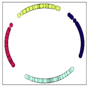
(a) R=1(Balanced)

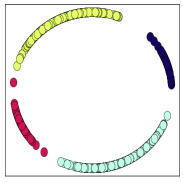
(b) R=4

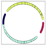
(c) R=16

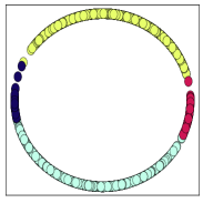
(d) R=64

Figure 6: Visualization of the embedding space learnt by vanilla contrastive learning loss on the 2-D imbalanced synthetic dataset with different imbalanced ratios (1,4,16,64). As the ratio increases, head classes gradually occupy the embedding space with the collapse of the tail classes.

Appendix F Additional Experimental Results and Further Analysis

F.1 Error Bars for the Main Results

In this part, we present main results with error bars calculated over 5 trials.

Table 12: Linear probing results (average accuracy, %) over 5 trials on CIFAR-LT with different imbalanced ratios (100,50,10), ImageNet-LT and Places-LT.

	CIFAR-LT-R100	CIFAR-LT-R50	CIFAR-LT-R10	ImageNet-LT	Places-LT
SimCLR	50.72$\pm$0.26	52.24$\pm$0.31	55.67$\pm$0.44	36.65$\pm$0.16	33.61$\pm$0.12
+GH	53.96$\pm$0.23	55.42$\pm$0.22	57.36$\pm$0.39	38.28$\pm$0.13	34.33$\pm$0.10
Focal	51.04$\pm$0.27	52.22$\pm$0.38	56.23$\pm$0.45	37.49$\pm$0.11	33.65$\pm$0.14
+GH	53.92$\pm$0.19	55.06$\pm$0.28	58.05$\pm$0.28	38.92$\pm$0.14	34.42$\pm$0.17
SDCLR	52.87$\pm$0.22	53.87$\pm$0.21	55.44$\pm$0.25	36.25$\pm$0.18	33.99$\pm$0.14
+GH	54.81$\pm$0.26	55.34$\pm$0.28	56.97$\pm$0.34	38.53$\pm$0.14	34.70$\pm$0.10
DnC	52.52$\pm$0.32	53.21$\pm$0.35	57.59$\pm$0.36	37.23$\pm$0.21	33.90$\pm$0.18
+GH	54.88$\pm$0.23	56.33$\pm$0.31	58.94$\pm$0.25	38.67$\pm$0.19	34.52$\pm$0.23
BCL	56.45$\pm$0.40	57.18$\pm$0.26	59.12$\pm$0.28	38.33$\pm$0.10	34.76$\pm$0.15
+GH	57.65$\pm$0.33	59.00$\pm$0.33	60.34$\pm$0.29	39.95$\pm$0.15	35.32$\pm$0.17

F.2 Convergence of the Surrogate Label Allocation

In Table 13, we provide the experiments to verify the convergence of the Sinkhorn-Knopp algorithm, which adopts the criterion as the stopping reference.

Table 13: The value of $e$ during the convergence of surrogate label allocation on CIFAR-LT-R100.

Iter	0	10	20	30	50	70	100	150
$e$	67.89	4.28	0.53	0.076	0.0054	0.0005	2.08$\times 10^{-5}$	3.58$\times 10^{-7}$

We define the criterion $e=sum(|u./u^{\prime}-1|)$ as the relative changes of one scaling vectors $u$, where $u^{\prime}$ represents the vector in the latest iteration. Then, the algorithm converges as the criterion $e\rightarrow 0$. As shown in Table 13, we can see that the criterion diminishes rapidly. Let $e<10^{-6}$ represent the indicator of the convergence, we further obtain the averaging convergence iterations as $141\pm 45$ (statistics under 1000 runs). In practice, we set the default Sinkhorn iterations as 300 to guarantee the convergence, as detailed in Section 4.1.

F.3 Empirical Comparison with More Baselines

In Table 14, we conduct a range of experiments to compare PMSN[35] and TS [2] with our proposed GH on CIFAR-LT with different imbalanced ratios.

Table 14: Linear probing accuracy of more SSL-LT baselines on CIFAR-100-LT with different imbalanced ratios.

	Method	Many	Med	Few	Avg
CIFAR-R100	SimCLR	54.97	49.39	47.67	50.72
	SimCLR+TS	55.53	50.33	50.06	52.01
	PMSN	55.62	52.12	49.85	52.56
	SimCLR+GH	57.38	52.27	52.12	53.96
	SimCLR+TS+GH	57.44	52.76	51.79	54.03
CIFAR-R50	SimCLR	56.00	50.48	50.12	52.24
	SimCLR+TS	56.44	52.58	51.91	53.67
	PMSN	56.76	52.52	53.09	54.15
	SimCLR+GH	58.88	53.00	54.27	55.42
	SimCLR+TS+GH	58.47	54.61	54.70	55.95
CIFAR-R10	SimCLR	57.85	55.06	54.03	55.67
	SimCLR+TS	58.26	56.24	54.97	56.51
	PMSN	56.91	54.61	55.67	55.74
	SimCLR+GH	59.26	56.91	55.85	57.36
	SimCLR+TS+GH	59.44	57.15	56.48	57.71

From the results, we can see that the proposed method consistently outperforms PMSN[35] and TS [2] across different imbalanced ratios on CIFAR-LT. Besides, we can observe that combining GH and TS [2] consistently improves the performance of contrastive learning on CIFAR-LT.

F.4 Empirical Comparison with K-Means Algorithm

K-means algorithm [22] tends to generate clusters with relatively uniform sizes, which will affect the cluster performance under the class-imbalanced scenarios [38]. To gain more insights, we conduct empirical comparisons using K-means as the clustering algorithm and evaluate the NMI score with ground-truth labels and the linear probing accuracy on CIFAR-LT-R100.

Table 15: Linear probing accuracy and NMI score on CIFAR-100-LT-R100.

Method	Accuracy	NMI score
SimCLR	50.72	0.28
+K-means	51.44	0.35
+GH	53.96	0.50

From the results, we can see that K-means generates undesired assignments with lower NMI score and achieves unsatisfying performance compared with our GH. This observation is consistent with previous studies [38].

F.5 Compatibility on the Class-Balanced Data

In Table 16, we present the results on the balanced dataset CIFAR-100 across different methods.

Table 16: Linear probing on class-balanced CIFAR-100. We report Accuracy($\%$) for comparison.

Method	SimCLR	+GH	Focal	+GH	SDCLR	+GH	DnC	+GH	BCL	+GH
Accuracy	66.75	66.41	66.42	66.79	65.46	66.17	67.78	67.57	69.16	69.33

From the results, we can see that GH shows comparable performance with the baseline methods when the data distribution is balanced. According to the neural collapse theory [49], well-trained neural networks can inherently produce the category-level uniformity on class-balanced data. As expected, our GH will degenerate to the vanilla SSL baselines as the geometric labels can easily be aligned with the latent ground-truth labels. The empirical findings are also consistent with recent explorations [31] in supervised learning context. Besides, the minor decrease in performance could potentially be attributed to some random factors during training or the negligible effect of GH loss as it might not reach an absolute zero value.

F.6 Computational Cost

In Table 17, we present the mini-batch training time of different baseline methods on CIFAR-100-LT, ImageNet-LT and Places-LT.

Table 17: The time cost (seconds) of mini-batch training on CIFAR-100-LT, ImageNet-LT and Places-LT.

Dataset	SimCLR	+GH	Focal	+GH	SDCLR	+GH	DnC	+GH	BCL	+GH
CIFAR-LT	0.38	0.41	0.37	0.40	0.42	0.47	0.39	0.41	0.38	0.41
ImageNet-LT	0.76	0.79	0.75	0.77	0.94	1.01	0.76	0.79	0.76	0.78
Places-LT	0.72	0.75	0.76	0.78	1.00	1.05	0.72	0.76	0.72	0.75

In our runs, the proposed GH only incurs a minor computational overhead on CIFAR-100-LT, ImageNet-LT and Places-LT, respectively, which is relatively lightweight compared to the total computational cost of the contrastive baselines. This indicates the great potential of GH to collaborate with more SSL methods to acquire the robustness on data imbalance in a low-cost manner.

F.7 Ablations on Hyper-parameters

In this part, we present ablation studies w.r.t. temperature $\gamma_{\mathrm{GH}}$, regularization coefficient $\lambda$ and Sinkhorn iteration $E_{s}$ on CIFAR-LT.

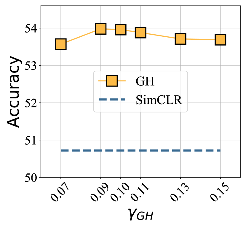
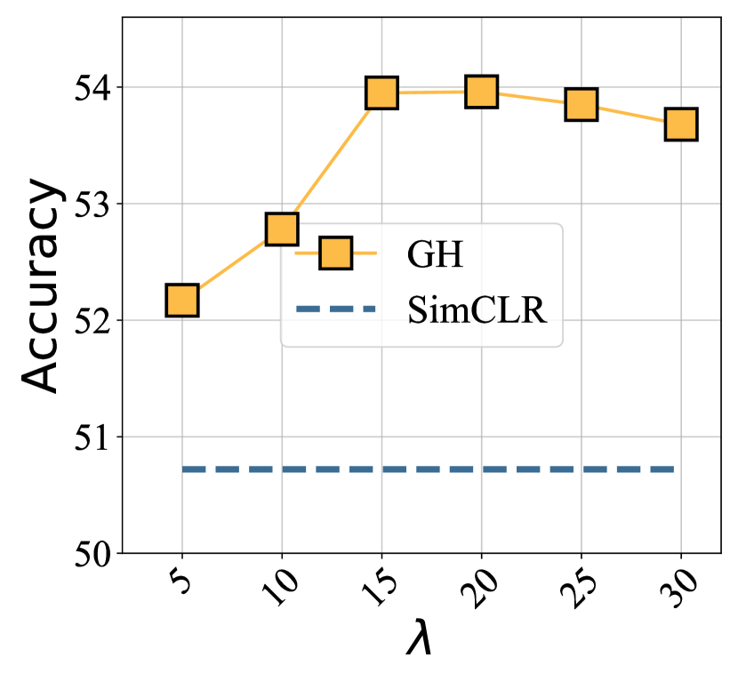
Figure 7: Ablations of temperature $\gamma_{\mathrm{GH}}$, coefficient $\lambda$ and Sinkhorn iteration $E_{s}$ on CIFAR-LT.

F.8 Ablations on the Training Epoch

In Table 18, we present the comparison between SimCLR and SimCLR+GH on CIFAR-LT-R100 under different training epochs.

Table 18: Linear probing results on CIFAR-LT-R100 with different training epochs.

epoch	200	500	1000	1500	2000
SimCLR	49.53	50.32	50.72	50.84	50.27
+GH	50.89	54.00	53.96	53.95	53.91

According to the table, we can see that both methods appropriately reach the saturated performance when the training epochs are larger than 500. To guarantee the converged performance, we thus set the default training epochs as 1000.

F.9 Ablations on the Batch Size

To explore the effect of the training batch size, we conduct the experiments with different batch size on CIFAR-LT-R100 as follows.

Table 19: Linear probing results on CIFAR-LT-R100 w.r.t the methods with different batch size.

Batch size	128	256	512	768	1024
SimCLR	50.14	51.08	50.72	50.25	50.07
+GH	52.72	53.43	53.96	53.95	53.18

Table 20: Linear probing results on ImageNet-LT w.r.t the methods with different batch size.

Batch size	256	384	512	768
SimCLR	36.65	36.97	37.85	38.04
+GH	38.28	39.22	41.06	41.34

From the results, we can see that our GH consistently outperforms the baseline SimCLR. It is worth noting that our method still provides siginificant improvements when the batch size is small (e.g. 2.6% with batch size as 128 on CIFAR-LT), which reflects the robustness of the proposed GH in terms of small batch sizes. Besides, we observe that the performance drops when reducing the batch size for both baseline method and our GH on CIFAR-LT and ImageNet-LT, as shown in Table 19. This can potentially be attributed to the higher probability of encountering situations where certain classes are missing under smaller batch size. Intuitively, it might easily generate biased estimation when there is no support for a certain class in the mini-batch. Then, the cluster quality might be affected by the probability of encountering missing class, which potentially correlates the important factor, i.e., batch size.

F.10 Ablations on Geometric Uniform Structure

In Table 21, we conduct experiments with the geometric uniform structure as the projector on top of the baseline contrastive learning methods. As can be seen, if geometric uniform structure alone is used to balance the representation learning, the improvement is minor and sometimes degrades. This is because the direct estimation from the geometric uniform structure is noisy during training when the representation is not ideally distributed.

Table 21: Ablations of the geometric uniform structure on CIFAR-100-LT with different imbalanced ratios (100, 50, 10).

Method	CIFAR-LT-R100	CIFAR-LT-R50	CIFAR-LT-R10
SimCLR	50.72	52.24	55.67
+GUS	51.10	51.99	55.56
+GH	53.96	55.42	57.36

F.11 Ablations on the Momentum Hyper-parameter

In our proposed GH, the hyper-parameter $\beta$ controls the smoothing degree on the historical statistics regarding the dynamically estimated surrogate label distribution $\bm{\pi}$. We conduct empirical comparison with different $\beta$ to validate the stability of our method, as depicted in Figure 8. From the results, we can see that our GH can achieve consistent performance at the most cases. To guarantee the performance, we thus set the default hyper-parameter $\beta$ as 0.999.

Figure 8: Linear probing w.r.t hyper-parameter $\beta$ on CIFAR-LT-R100.

F.12 Implementations of Geometric Uniform Structure

In Figure 9, we empirically compare the results of analytical geometric uniform structure (Simplex ETF) with those of proxy variants. We thus conduct the sensitivity analysis w.r.t a smaller span of K, ranging from 30 to 220. From the results, we observe that the comparable performance is achieved in both geometric structures. This indicates that our method is effective to two forms of the geometric structure, relaxing the hard dimensional constraints in the analytical solution. It is also worth noting that our method’s efficacy remains unaffected by the dimension of the geometric uniform structure when appropriately choosing the dimension, highlighting its ease of application.

Figure 9: Linear probing performance w.r.t. the dimension $K$ of the geometric uniform structure $\mathbf{M}$ on CIFAR-LT-R100. Analytical or approximate solution are applied according to the dimensional constraints. More details can be referred to Appendix B.

F.13 Full-shot Evaluation on Large-scale Dataset

Here we provide 100-shot evaluation and full-shot evaluation on ImageNet-LT, as shown in Table 22. We observe that the performance improvements and representation balancedness (Std) are consistent with both evaluations, indicating the rationality of the 100-shot evaluation.

Table 22: Full-shot linear evaluation and 100-shot evaluation on ImageNet-LT.

Evaluation	Method	Many	Medium	Few	Std	Avg
100-shot	SimCLR	41.69	33.96	31.82	5.19	36.65
	+GH	41.53	36.35	35.84	3.15	38.28
Full-shot	SimCLR	42.86	35.17	33.13	5.13	37.86
	+GH	44.11	38.59	37.87	3.41	40.62

F.14 Comprehensive Evaluation on More Real-world Scenarios

To further validate the generalization of the proposed method, we conduct more comprehensive comparisons on various datasets with distinct characteristics and tasks, and conduct more experiments as follows:

• Marine-tree dataset [3]: This dataset is a large-scale dataset for marine organism classification. It contains more than 160K images divided into 60 classes with the number of images per class ranging from 14 to 16761.

• IMDB-WIKI-DIR dataset [69]: IMDB-WIKI-DIR (age) dataset is subsampled from IMDB-WIKI dataset [51] to construct the deep imbalanced regression benchmark. It contains 202.5K images with the number of images per bin varied between 1 and 7149.

• CUB-200 [61] and Aircrafts [45] dataset. Caltech-UCSD Birds 200 (CUB-200) and Aircrafts dataset are two fine-grained datasets, which contains 11K images with 200 classes and 10K images with 102 classes, respectively.

Table 23: Linear probing results (average accuracy, %) on Marine-tree dataset.

Marine	Many	Medium	Few	Avg
SimCLR	36.05	47.01	48.80	43.95
+GH	35.70	47.14	51.62	44.82

Table 24: Vanilla finetuning results under the metric of mean average error (MAE [69], lower is better) on IMDB-WIKI-DIR dataset.

IMDB-WIKI-DIR (MAE)	Many	Medium	Few	Avg
SimCLR	8.10	18.31	29.99	9.14
+GH	7.77	17.18	29.29	8.75

Table 25: Vanilla finetuning results under the metric of Geometric Mean (GM [69], lower is better) on IMDB-WIKI-DIR dataset.

IMDB-WIKI-DIR (GM)	Many	Medium	Few	Avg
SimCLR	4.87	15.01	26.61	5.43
+GH	4.64	13.49	24.54	5.14

Table 26: Downstream linear probing results (Top1/Top5 accuracy, %) on CUB-200 dataset.

CUB-200	SimCLR	+GH	Focal	+GH	SDCLR	+GH	DnC	+GH	BCL	+GH
TOP1	28.97	29.89	30.13	30.68	28.98	29.63	29.64	30.46	28.46	28.97
TOP5	57.28	57.92	58.01	58.78	57.34	57.95	57.63	58.55	56.92	57.66

Table 27: Downstream linear probing results (Top1/Top5 accuracy, %) on Aircrafts dataset.

Aircrafts	SimCLR	+GH	Focal	+GH	SDCLR	+GH	DnC	+GH	BCL	+GH
TOP1	29.82	30.63	31.02	31.74	30.99	31.85	31.18	32.05	32.79	35.88
TOP5	56.14	57.95	57.82	58.99	58.09	59.13	58.11	59.42	60.79	63.34

On large-scale dataset (Marine-tree dataset and IMDB-WIKI-DIR dataset), we adopt the training schedule similar to ImageNet-LT and Places-LT, except the training epochs reduced from 500 to about 200 epochs. Besides, we crop the images with the low resolution (112x112) to speed up the training. We conduct linear probing on Marine-tree, CUB-200 and Aircrafts dataset. The former is pretrained with Marine-tree dataset, while the latter is pretrained with ImageNet-LT. As for IMDB-WIKI-DIR dataset, we pretrain the network for initializing the weights of the downstream supervised imbalanced regression task. Specially, the geometric mean (GM) is defined for better prediction fairness [69]. Both the evaluation metrics (MAE, GM) are the smaller the better.

From the results in Tables 23, 24, 25, 26 and 27, we can see that our proposed GH consistently outperforms the baseline methods for all the metrics (linear probing accuracy, finetuning accuracy, MAE and GM) on various datasets/settings. This indicates the potential of GH for adapting to a wide range of real-world data scenarios to counteract the negative impact of the long-tailed distribution.

F.15 More Results on Joint Optimization with Warm-up Strategy

We can potentially adopt warm-up strategy to initialize the weights $\theta$ against the degenerate solutions in the joint optimization. In this subsection, we conduct more comprehenvive experiments on CIFAR-LT-100 with different warm-up epochs to further verify the superiority of the proposed bi-level optimization.

Table 28: Linear probing results of joint optimization on CIFAR-LT-R100 with different warm-up epochs.

Epoch	0	10	50	100	200	300	400
Accuracy	50.18	51.14	50.77	50.97	50.44	50.21	50.57

From the results in Table 28, we can see that the warm-up strategy has the potential to improve the linear probing performance by 1% over the vanilla joint training. However, it seems that this strategy is sensitive to the proper epochs for warming-up, and the overall performance is not better than the bi-level optimization.

Appendix G Broader Impacts

Learning long-tailed data without annotations is a vital element in the deployment of robust deep learning systems in the real-world applications [25, 76, 72, 73]. The attribution is that real-world natural resources inevitably exhibit the long-tailed distribution [50]. The importance of self-supervised long-tailed learning is further emphasized when extended to a range of safety-critical scenarios [8, 26, 27], including medical intelligence [65, 66, 74], autonomous driving [55, 56, 57] and criminal surveillance, where the data imbalance may lead to the distorted representation. In this paper, we study a general and practical research problem in representation learning parity for self-supervised long-tailed learning, considering the intrinsic limitation of conventional contrastive learning that can not adequately address the over-expansion of the majorities and the passive-collapse of the minorities in the embedding space. Our method regularizes long-tailed learning from a geometric perspective and motivates more benign representation, which helps improve the downstream generalization and representation balancedness. Besides, our method has the potential to be applied in fairness research scenarios [42] where both majority and minority classes (or attributes) are present. Given the guidance of label information, we can explicitly constrain a consistent embedding space for each subgroup, thereby promoting category-level uniformity.

Nevertheless, it is important to acknowledge that our method may have negative impact, such as employment disruption, as our study endeavors to reduce annotation costs by enabling robust self-supervised learning on hard-to-collect tail data resources. Specially, if self-supervised learning can extract the tail distribution with sufficient accuracy, the necessity for the human manipulation on the quality of data distribution will diminish.

Appendix H Limitations

Roughly, our design is built upon the intrinsic clustering patterns that can inclusively represent the information for the downstream tasks. Although we demonstrate the appealing performance in the current benchmark, it cannot be always guaranteed in all scenarios. Once such a condition is not satisfied, namely, clustering only captures the task-irrelevant patterns but ignores the task-relevant details, the improvement might be limited or even negative. A potential way to overcome this drawback is using a small auxiliary labeling set to calibrate the clustering dynamic aligned with the downstream tasks, namely, a semi-supervised paradigm. The methods to encourage learning the stable features in the area of causal inference can also be borrowed to this problem to alleviate this dilemma.

References

- Asano et al. [2020] Yuki M. Asano, Christian Rupprecht, and Andrea Vedaldi. Self-labelling via simultaneous clustering and representation learning. In International Conference on Learning Representations (ICLR), 2020.
- Assran et al. [2023] Mido Assran, Randall Balestriero, Quentin Duval, Florian Bordes, Ishan Misra, Piotr Bojanowski, Pascal Vincent, Michael Rabbat, and Nicolas Ballas. The hidden uniform cluster prior in self-supervised learning. In The Eleventh International Conference on Learning Representations, 2023.
- Boone-Sifuentes et al. [2022] Tanya Boone-Sifuentes, Asef Nazari, Imran Razzak, Mohamed Reda Bouadjenek, Antonio Robles-Kelly, Daniel Ierodiaconou, and Elizabeth S Oh. Marine-tree: A large-scale marine organisms dataset for hierarchical image classification. In Proceedings of the 31st ACM International Conference on Information & Knowledge Management, pages 3838–3842, 2022.
- Borodachov et al. [2019] Sergiy V Borodachov, Douglas P Hardin, and Edward B Saff. Discrete energy on rectifiable sets. Springer, 2019.
- Cao et al. [2019] Kaidi Cao, Colin Wei, Adrien Gaidon, Nikos Arechiga, and Tengyu Ma. Learning imbalanced datasets with label-distribution-aware margin loss. Advances in Neural Information Processing Systems, 32:1567–1578, 2019.
- Caron et al. [2018] Mathilde Caron, Piotr Bojanowski, Armand Joulin, and Matthijs Douze. Deep clustering for unsupervised learning of visual features. In Proceedings of the European conference on computer vision (ECCV), pages 132–149, 2018.
- Caron et al. [2020] Mathilde Caron, Ishan Misra, Julien Mairal, Priya Goyal, Piotr Bojanowski, and Armand Joulin. Unsupervised learning of visual features by contrasting cluster assignments. Advances in Neural Information Processing Systems, 33:9912–9924, 2020.
- Chen et al. [2023] Mengxi Chen, Linyu Xing, Yu Wang, and Ya Zhang. Enhanced multimodal representation learning with cross-modal kd. In Proceedings of the IEEE/CVF Conference on Computer Vision and Pattern Recognition, pages 11766–11775, 2023.
- Chen et al. [2020] Ting Chen, Simon Kornblith, Mohammad Norouzi, and Geoffrey Hinton. A simple framework for contrastive learning of visual representations. In International Conference on Machine Learning, pages 1597–1607. PMLR, 2020.
- Chen and He [2021] Xinlei Chen and Kaiming He. Exploring simple siamese representation learning. In Proceedings of the IEEE/CVF Conference on Computer Vision and Pattern Recognition, pages 15750–15758, 2021.
- Chen* et al. [2021] Xinlei Chen*, Saining Xie*, and Kaiming He. An empirical study of training self-supervised vision transformers. arXiv preprint arXiv:2104.02057, 2021.
- Cohn and Kumar [2007] Henry Cohn and Abhinav Kumar. Universally optimal distribution of points on spheres. Journal of the American Mathematical Society, 20(1):99–148, 2007.
- Cui et al. [2021] Jiequan Cui, Zhisheng Zhong, Shu Liu, Bei Yu, and Jiaya Jia. Parametric contrastive learning. In Proceedings of the IEEE/CVF International Conference on Computer Vision, pages 715–724, 2021.
- Cuturi [2013] Marco Cuturi. Sinkhorn distances: Lightspeed computation of optimal transport. Advances in neural information processing systems, 26, 2013.
- Doersch et al. [2015] Carl Doersch, Abhinav Gupta, and Alexei A Efros. Unsupervised visual representation learning by context prediction. In Proceedings of the IEEE International Conference on Computer Vision, pages 1422–1430, 2015.
- Fan et al. [2022] Ziqing Fan, Yanfeng Wang, Jiangchao Yao, Lingjuan Lyu, Ya Zhang, and Qi Tian. Fedskip: Combatting statistical heterogeneity with federated skip aggregation. In 2022 IEEE International Conference on Data Mining (ICDM), pages 131–140. IEEE, 2022.
- Fang et al. [2021] Cong Fang, Hangfeng He, Qi Long, and Weijie J Su. Exploring deep neural networks via layer-peeled model: Minority collapse in imbalanced training. Proceedings of the National Academy of Sciences, 118(43):e2103091118, 2021.
- Garrido et al. [2023] Quentin Garrido, Yubei Chen, Adrien Bardes, Laurent Najman, and Yann LeCun. On the duality between contrastive and non-contrastive self-supervised learning. In The Eleventh International Conference on Learning Representations, 2023.
- Graf et al. [2021] Florian Graf, Christoph Hofer, Marc Niethammer, and Roland Kwitt. Dissecting supervised constrastive learning. In International Conference on Machine Learning, pages 3821–3830. PMLR, 2021.
- Grill et al. [2020] Jean-Bastien Grill, Florian Strub, Florent Altché, Corentin Tallec, Pierre Richemond, Elena Buchatskaya, Carl Doersch, Bernardo Avila Pires, Zhaohan Guo, Mohammad Gheshlaghi Azar, et al. Bootstrap your own latent-a new approach to self-supervised learning. Advances in neural information processing systems, 33:21271–21284, 2020.
- Hardin and Saff [2005] DP Hardin and EB Saff. Minimal riesz energy point configurations for rectifiable d-dimensional manifolds. Advances in Mathematics, 193(1):174–204, 2005.
- Hartigan and Wong [1979] John A Hartigan and Manchek A Wong. Algorithm as 136: A k-means clustering algorithm. Journal of the royal statistical society. series c (applied statistics), 28(1):100–108, 1979.
- He et al. [2016] Kaiming He, Xiangyu Zhang, Shaoqing Ren, and Jian Sun. Deep residual learning for image recognition. In Proceedings of the IEEE Conference on Computer Vision and Pattern Recognition, pages 770–778, 2016.
- He et al. [2020] Kaiming He, Haoqi Fan, Yuxin Wu, Saining Xie, and Ross Girshick. Momentum contrast for unsupervised visual representation learning. In Proceedings of the IEEE/CVF Conference on Computer Vision and Pattern Recognition, pages 9729–9738, 2020.
- Hong et al. [2023] Feng Hong, Jiangchao Yao, Zhihan Zhou, Ya Zhang, and Yanfeng Wang. Long-tailed partial label learning via dynamic rebalancing. In The Eleventh International Conference on Learning Representations, 2023.
- Huang et al. [2022a] Chaoqin Huang, Haoyan Guan, Aofan Jiang, Ya Zhang, Michael Spratling, and Yan-Feng Wang. Registration based few-shot anomaly detection. In European Conference on Computer Vision, pages 303–319. Springer, 2022a.
- Huang et al. [2022b] Chaoqin Huang, Qinwei Xu, Yanfeng Wang, Yu Wang, and Ya Zhang. Self-supervised masking for unsupervised anomaly detection and localization. IEEE Transactions on Multimedia, 2022b.
- Jiang et al. [2021] Ziyu Jiang, Tianlong Chen, Bobak J Mortazavi, and Zhangyang Wang. Self-damaging contrastive learning. In International Conference on Machine Learning, pages 4927–4939. PMLR, 2021.
- Kang et al. [2019] Bingyi Kang, Saining Xie, Marcus Rohrbach, Zhicheng Yan, Albert Gordo, Jiashi Feng, and Yannis Kalantidis. Decoupling representation and classifier for long-tailed recognition. In International Conference on Learning Representations, 2019.
- Kang et al. [2020] Bingyi Kang, Yu Li, Sa Xie, Zehuan Yuan, and Jiashi Feng. Exploring balanced feature spaces for representation learning. In International Conference on Learning Representations, 2020.
- Kasarla et al. [2022] Tejaswi Kasarla, Gertjan Burghouts, Max van Spengler, Elise van der Pol, Rita Cucchiara, and Pascal Mettes. Maximum class separation as inductive bias in one matrix. In Advances in Neural Information Processing Systems, volume 35, pages 19553–19566, 2022.
- Khosla et al. [2011] Aditya Khosla, Nityananda Jayadevaprakash, Bangpeng Yao, and Fei-Fei Li. Novel dataset for fine-grained image categorization: Stanford dogs. In Proc. CVPR Workshop on Fine-Grained Visual Categorization (FGVC), volume 2. Citeseer, 2011.
- Krause et al. [2013] Jonathan Krause, Michael Stark, Jia Deng, and Li Fei-Fei. 3d object representations for fine-grained categorization. In Proceedings of the IEEE international conference on computer vision workshops, pages 554–561, 2013.
- Krizhevsky [2009] A Krizhevsky. Learning multiple layers of features from tiny images. Technical Report TR-2009, University of Toronto, 2009.
- Kukleva et al. [2023] Anna Kukleva, Moritz Böhle, Bernt Schiele, Hilde Kuehne, and Christian Rupprecht. Temperature schedules for self-supervised contrastive methods on long-tail data. In The Eleventh International Conference on Learning Representations, 2023.
- Li et al. [2021] Junnan Li, Pan Zhou, Caiming Xiong, and Steven Hoi. Prototypical contrastive learning of unsupervised representations. In International Conference on Learning Representations, 2021.
- Li et al. [2022] Tianhong Li, Peng Cao, Yuan Yuan, Lijie Fan, Yuzhe Yang, Rogerio S Feris, Piotr Indyk, and Dina Katabi. Targeted supervised contrastive learning for long-tailed recognition. In Proceedings of the IEEE/CVF Conference on Computer Vision and Pattern Recognition, pages 6918–6928, 2022.
- Liang et al. [2012] Jiye Liang, Liang Bai, Chuangyin Dang, and Fuyuan Cao. The -means-type algorithms versus imbalanced data distributions. IEEE Transactions on Fuzzy Systems, 20(4):728–745, 2012.
- Lin et al. [2014] Tsung-Yi Lin, Michael Maire, Serge Belongie, James Hays, Pietro Perona, Deva Ramanan, Piotr Dollár, and C Lawrence Zitnick. Microsoft coco: Common objects in context. In Computer Vision–ECCV 2014: 13th European Conference, Zurich, Switzerland, September 6-12, 2014, Proceedings, Part V 13, pages 740–755. Springer, 2014.
- Lin et al. [2017] Tsung-Yi Lin, Priya Goyal, Ross Girshick, Kaiming He, and Piotr Dollár. Focal loss for dense object detection. In Proceedings of the IEEE International Conference on Computer Vision, pages 2980–2988, 2017.
- Liu et al. [2021] Hong Liu, Jeff Z HaoChen, Adrien Gaidon, and Tengyu Ma. Self-supervised learning is more robust to dataset imbalance. In International Conference on Learning Representations, 2021.
- Liu et al. [2017] Weiyang Liu, Yandong Wen, Zhiding Yu, Ming Li, Bhiksha Raj, and Le Song. Sphereface: Deep hypersphere embedding for face recognition. In Proceedings of the IEEE conference on computer vision and pattern recognition, pages 212–220, 2017.
- Liu et al. [2018] Weiyang Liu, Rongmei Lin, Zhen Liu, Lixin Liu, Zhiding Yu, Bo Dai, and Le Song. Learning towards minimum hyperspherical energy. Advances in neural information processing systems, 31, 2018.
- Liu et al. [2019] Ziwei Liu, Zhongqi Miao, Xiaohang Zhan, Jiayun Wang, Boqing Gong, and Stella X Yu. Large-scale long-tailed recognition in an open world. In Proceedings of the IEEE/CVF Conference on Computer Vision and Pattern Recognition, pages 2537–2546, 2019.
- Maji et al. [2013] Subhransu Maji, Esa Rahtu, Juho Kannala, Matthew Blaschko, and Andrea Vedaldi. Fine-grained visual classification of aircraft. arXiv preprint arXiv:1306.5151, 2013.
- Menon et al. [2021] Aditya Krishna Menon, Sadeep Jayasumana, Ankit Singh Rawat, Himanshu Jain, Andreas Veit, and Sanjiv Kumar. Long-tail learning via logit adjustment. In International Conference on Learning Representations, 2021.
- Mixon et al. [2022] Dustin G Mixon, Hans Parshall, and Jianzong Pi. Neural collapse with unconstrained features. Sampling Theory, Signal Processing, and Data Analysis, 20(2):1–13, 2022.
- Oord et al. [2018] Aaron van den Oord, Yazhe Li, and Oriol Vinyals. Representation learning with contrastive predictive coding. arXiv preprint arXiv:1807.03748, 2018.
- Papyan et al. [2020] Vardan Papyan, XY Han, and David L Donoho. Prevalence of neural collapse during the terminal phase of deep learning training. Proceedings of the National Academy of Sciences, 117(40):24652–24663, 2020.
- Reed [2001] William J Reed. The pareto, zipf and other power laws. Economics letters, 74(1):15–19, 2001.
- Rothe et al. [2018] Rasmus Rothe, Radu Timofte, and Luc Van Gool. Deep expectation of real and apparent age from a single image without facial landmarks. International Journal of Computer Vision, 126(2-4):144–157, 2018.
- Sharma et al. [2018] Piyush Sharma, Nan Ding, Sebastian Goodman, and Radu Soricut. Conceptual captions: A cleaned, hypernymed, image alt-text dataset for automatic image captioning. In Proceedings of the 56th Annual Meeting of the Association for Computational Linguistics (Volume 1: Long Papers), pages 2556–2565, 2018.
- Smale [1998] Steve Smale. Mathematical problems for the next century. The mathematical intelligencer, 20(2):7–15, 1998.
- Strehl and Ghosh [2002] Alexander Strehl and Joydeep Ghosh. Cluster ensembles—a knowledge reuse framework for combining multiple partitions. Journal of machine learning research, 3(Dec):583–617, 2002.
- Sun et al. [2021] Jianhua Sun, Yuxuan Li, Hao-Shu Fang, and Cewu Lu. Three steps to multimodal trajectory prediction: Modality clustering, classification and synthesis. In Proceedings of the IEEE/CVF International Conference on Computer Vision, pages 13250–13259, 2021.
- Sun et al. [2022] Jianhua Sun, Yuxuan Li, Liang Chai, Hao-Shu Fang, Yong-Lu Li, and Cewu Lu. Human trajectory prediction with momentary observation. In Proceedings of the IEEE/CVF Conference on Computer Vision and Pattern Recognition, pages 6467–6476, 2022.
- Sun et al. [2023] Jianhua Sun, Yuxuan Li, Liang Chai, and Cewu Lu. Modality exploration, retrieval and adaptation for trajectory prediction. IEEE Transactions on Pattern Analysis and Machine Intelligence, 2023.
- Thomson [1904] Joseph John Thomson. Xxiv. on the structure of the atom: an investigation of the stability and periods of oscillation of a number of corpuscles arranged at equal intervals around the circumference of a circle; with application of the results to the theory of atomic structure. The London, Edinburgh, and Dublin Philosophical Magazine and Journal of Science, 7(39):237–265, 1904.
- Tian et al. [2021] Yonglong Tian, Olivier J Henaff, and Aäron van den Oord. Divide and contrast: Self-supervised learning from uncurated data. In Proceedings of the IEEE/CVF International Conference on Computer Vision, pages 10063–10074, 2021.
- Van Horn et al. [2015] Grant Van Horn, Steve Branson, Ryan Farrell, Scott Haber, Jessie Barry, Panos Ipeirotis, Pietro Perona, and Serge Belongie. Building a bird recognition app and large scale dataset with citizen scientists: The fine print in fine-grained dataset collection. In Proceedings of the IEEE Conference on Computer Vision and Pattern Recognition, pages 595–604, 2015.
- Wah et al. [2011] Catherine Wah, Steve Branson, Peter Welinder, Pietro Perona, and Serge Belongie. The caltech-ucsd birds-200-2011 dataset. 2011.
- Wang and Isola [2020] Tongzhou Wang and Phillip Isola. Understanding contrastive representation learning through alignment and uniformity on the hypersphere. In International Conference on Machine Learning, pages 9929–9939. PMLR, 2020.
- Wang and Gupta [2015] Xiaolong Wang and Abhinav Gupta. Unsupervised learning of visual representations using videos. In Proceedings of the IEEE International Conference on Computer Vision, pages 2794–2802, 2015.
- Wang et al. [2021] Yifei Wang, Qi Zhang, Yisen Wang, Jiansheng Yang, and Zhouchen Lin. Chaos is a ladder: A new theoretical understanding of contrastive learning via augmentation overlap. In International Conference on Learning Representations, 2021.
- Wu et al. [2022] Chaoyi Wu, Feng Chang, Xiao Su, Zhihan Wu, Yanfeng Wang, Ling Zhu, and Ya Zhang. Integrating features from lymph node stations for metastatic lymph node detection. Computerized Medical Imaging and Graphics, 101:102108, 2022.
- Wu et al. [2023] Chaoyi Wu, Xiaoman Zhang, Ya Zhang, Yanfeng Wang, and Weidi Xie. Towards generalist foundation model for radiology. arXiv preprint arXiv:2308.02463, 2023.
- Yang et al. [2022] Yibo Yang, Liang Xie, Shixiang Chen, Xiangtai Li, Zhouchen Lin, and Dacheng Tao. Do we really need a learnable classifier at the end of deep neural network? arXiv preprint arXiv:2203.09081, 2022.
- Yang and Xu [2020] Yuzhe Yang and Zhi Xu. Rethinking the value of labels for improving class-imbalanced learning. Advances in neural information processing systems, 33:19290–19301, 2020.
- Yang et al. [2021] Yuzhe Yang, Kaiwen Zha, Yingcong Chen, Hao Wang, and Dina Katabi. Delving into deep imbalanced regression. In International Conference on Machine Learning, pages 11842–11851. PMLR, 2021.
- Yao et al. [2023] Jiangchao Yao, Bo Han, Zhihan Zhou, Ya Zhang, and Ivor W Tsang. Latent class-conditional noise model. IEEE Transactions on Pattern Analysis and Machine Intelligence, 2023.
- Zbontar et al. [2021] Jure Zbontar, Li Jing, Ishan Misra, Yann LeCun, and Stéphane Deny. Barlow twins: Self-supervised learning via redundancy reduction. In International Conference on Machine Learning, pages 12310–12320. PMLR, 2021.
- Zhang et al. [2021a] Fei Zhang, Lei Feng, Bo Han, Tongliang Liu, Gang Niu, Tao Qin, and Masashi Sugiyama. Exploiting class activation value for partial-label learning. In International Conference on Learning Representations, 2021a.
- Zhang et al. [2021b] Fei Zhang, Chaochen Gu, Chenyue Zhang, and Yuchao Dai. Complementary patch for weakly supervised semantic segmentation. In Proceedings of the IEEE/CVF international conference on computer vision, pages 7242–7251, 2021b.
- Zhang et al. [2023a] Ruipeng Zhang, Ziqing Fan, Qinwei Xu, Jiangchao Yao, Ya Zhang, and Yanfeng Wang. Grace: A generalized and personalized federated learning method for medical imaging. In International Conference on Medical Image Computing and Computer-Assisted Intervention, pages 14–24. Springer, 2023a.
- Zhang et al. [2023b] Yifan Zhang, Bingyi Kang, Bryan Hooi, Shuicheng Yan, and Jiashi Feng. Deep long-tailed learning: A survey. IEEE Transactions on Pattern Analysis and Machine Intelligence, 2023b.
- Zhou et al. [2023] Yuhang Zhou, Jiangchao Yao, Feng Hong, Ya Zhang, and Yanfeng Wang. Balanced destruction-reconstruction dynamics for memory-replay class incremental learning. arXiv preprint arXiv:2308.01698, 2023.
- Zhou et al. [2022] Zhihan Zhou, Jiangchao Yao, Yan-Feng Wang, Bo Han, and Ya Zhang. Contrastive learning with boosted memorization. In International Conference on Machine Learning, pages 27367–27377. PMLR, 2022.
- Zhu et al. [2021] Zhihui Zhu, Tianyu Ding, Jinxin Zhou, Xiao Li, Chong You, Jeremias Sulam, and Qing Qu. A geometric analysis of neural collapse with unconstrained features. Advances in Neural Information Processing Systems, 34:29820–29834, 2021.
Appendix: Combating Representation Learning Disparity with Geometric Harmonization