2-Form U(1) Spin Liquids: Classical Model and Quantum Aspects

Abstract

We introduce a novel geometrically frustrated classical Ising model, dubbed the “spin vorticity model”, whose ground state manifold is a novel classical spin liquid: a 2-form Coulomb phase. We study the thermodynamics of this model both analytically and numerically, exposing the presence of algebraically decaying correlations and an extensive ground state entropy, and give a comprehensive account of its ground state properties and excitations. Each classical ground state may be decomposed into collections of closed 2-dimensional membranes, supporting fractionalized string excitations attached to the edges of open membranes. At finite temperature, the model can then be described as a gas of closed strings in a background of fluctuating membranes. The emergent gauge structure of this spin liquid is naturally couched in the language of 2-form electrodynamics, which describes 1-dimensional charged strings coupled to a rank-2 anti-symmetric gauge field. After establishing the classical spin vorticity model, we consider perturbing it with quantum exchange interactions, deriving an effective “membrane exchange” model of the quantum dynamics, analogous to ring exchange in quantum spin ice. We demonstrate the existence of a Rokhsar-Kivelson point where the quantum ground state is an equal-weight superposition of all classical ground state configurations, i.e. a quantum spin liquid. The quantum aspects of this spin liquid are exposed by mapping the membrane exchange model to a strongly-coupled frustrated 2-form U(1) lattice gauge theory. We further demonstrate how to quantize the string excitations by coupling a 1-form string field to the 2-form U(1) gauge field, thus mapping a quantum spin model to a 2-form U(1) gauge-Higgs model. We discuss the stability of the gapless deconfined phase of this gauge theory and the possibility of realizing a novel class of quantum phases of matter: 2-form U(1) quantum spin liquids.

I Introduction

A central aim of modern condensed matter physics is the search for and classification of novel phases of matter which challenge traditional notions of order and symmetry breaking [1, 2]. Some of the most experimentally promising routes to realizing such “beyond-Landau” possibilities are spin liquids—magnetic phases in which long-range order is evaded due to strong frustration caused by competing interactions. At the classical level, spin liquids are described by a massively degenerate ground state manifold with an emergent gauge structure and fractionalized excitations [3]. At the quantum level, the ground state of a quantum spin liquid (QSL) is a highly entangled superposition of such classical ground states [4, 5, 6, 7, 8]. Theoretically, QSLs are characterized by emergent gauge fields, which mediate the interactions of deconfined fractionalized excitations [7, 6, 5]. These can be roughly divided into those with a discrete gauge group, which are usually gapped, and those whose gauge group is U(1), which are generically gapless [7]. In the latter case, the gapless excitations may be identified as emergent or “artificial” photons [7, 9].

While in two dimensions we are furnished with a plethora of models which admit exact or near-exact solutions, such as the toric code [10] or Kitaev model [11], the situation for three-dimensional U(1) QSLs is significantly less ideal, with a paucity of cases for which we can conclusively identify quantum spin liquids starting from a realistic microscopic spin model. Significant effort has gone to classification of mean field ground states based on parton ansätze of quasiparticles interacting with a gapless photon [12, 13, 14, 15, 16, 17]. While these classification results are powerful, it remains desirable to have microscopic three-dimensional spin models from which we can directly derive the emergent gauge theory without resorting to either a quasiparticle ansatz or parton mean field approximation.

In this endeavor, the pyrochlore lattice of corner-sharing tetrahedra (Fig. 1(a)) serves as the premier platform for the study of frustrated magnetism and spin liquidity in three dimensions, with a rich interplay of theoretical and experimental developments [18, 19, 20]. In particular, it hosts a U(1) QSL called quantum spin ice (QSI) [21], one of very few 3D QSL’s with a detailed microscopic picture. The QSI phase arises by perturbing the microscopic classical nearest-neighbor spin ice (NNSI) model, with off-diagonal quantum exchange interactions [21, 9, 22, 23, 24]. NNSI is an exemplar model of classical spin liquidity, whose strongly-correlated behavior arises from the geometrically frustrated corner-sharing geometry of the pyrochlore lattice [25]. The classical Ising Hamiltonian imposes a local microscopic constraint on every tetrahedron, such that the low-temperature phase is described by a coarse-grained vector field $\bm{E}$ satisfying a divergence-free condition, $\cramped{\nabla\cdot\bm{E}=0}$ [25, 21, 3, 26, 27, 28, 29]. These local constraints leave a highly-degenerate ground state manifold, in which spins collectively align in a head-to-tail fashion to form a network of closed strings [29, 28, 27], referred to as a Coulomb phase [3, 27] or string condensate [30]. This phase manifests itself in momentum-resolved correlation functions as characteristic “pinch point” singularities [31, 25]. Point-like quasiparticle excitations (spinons) then appear at the ends of open strings of spins, acting as local “electric charges” $Q$ sourcing the divergence of $\bm{E}$ via an emergent Gauss law, $\cramped{\nabla\cdot\bm{E}=Q}$ [28, 32, 33]. Upon quantization, the quantum fluctuations of these strings become a collective gapless photon excitation described by an emergent U(1) gauge field [9, 34, 21]. Thus quantum spin ice realizes emergent quantum electrodynamics (QED), with electric charges (spinons), magnetic monopoles (visons) [9], a gapless photon and an associated fine structure constant [35].

In addition to spin ice, the pyrochlore lattice has been found to host additional spin liquid phases by considering anisotropic spin-spin interactions in the full symmetry-allowed nearest-neighbor pseudospin Hamiltonian [20]. Within the classical phase diagram of this model [36] one may find, in addition to spin ice, the Heisenberg antiferromagnet [25, 31, 26] and so-called pseudo-Heisenberg antiferromagnet [37], both of which are described by three decoupled Coulomb phases. Additionally, two “exotic” spin liquids have been identified—the so-called “pinch-line spin liquid” [38] and the “rank-2 U(1) spin liquid” [39], both of which are described in the coarse-grained approximation by emergent tensor gauge fields. The latter is of particularly broad interest, because it is described by a symmetric rank-2 tensor gauge field, which are fundamental to theories of fractons [40], excitations that can only move on subdimensional spaces [41, 42, 43], which have close connections to the theory of elasticity [44] and linearized gravity [45, 46]. For all of these classical spin liquids arising from nearest-neighbor spin models on the pyrochlore lattice, the essential physics can be understood as a consequence of local constraints enforced on each tetrahedron, which endow the system with a very large highly-correlated ground state manifold. In principle, quantum fluctuations may turn these classical spin liquids into exotic QSLs. However, to do so in a controlled manner, one would generally hope to construct a map from the microscopic spin model to an appropriate lattice gauge theory, as can be done to study quantum spin ice [9, 24]. Unfortunately such a map is currently not known for the pinch-line spin liquid or rank-2 U(1) spin liquid models, and it is desirable to find exotic spin liquids for which such an analysis can be carried out.

In each of the pyrochlore spin liquids discussed thus far, violations of the local constraints may be viewed as charges localized at the center of a tetrahedron. Even in the “exotic” tensor spin liquids, the excitations are zero-dimensional charged quasiparticles coupled to gauge fields by emergent Gauss laws, i.e. the charge density acts as the source of an appropriate divergence of the gauge field [8]. One may then wonder whether there are spin liquid phases falling beyond the framework of point-like quasiparticles coupled by a Gauss law to a gauge field. Upon brief thought, taking inspiration from Maxwell electromagnetism, we are presented with another possibility: replacing the Gauss law with an emergent Ampere-like law. This idea might seem peculiar at first glance—the Gauss law is a constraint enforced by gauge symmetry, while the Ampere’s law is a dynamical consequence of the equations of motion. However, from a field theory point of view, this does not prevent us from asking a simple question: can a three-dimensional classical spin liquid exist described by an emergent coarse-grained vector field ${\bm{E}}$ with a suppressed curl, ${\nabla\times\bm{E}=0}$, and if so, what happens when one adds quantum fluctuations to it? Such a spin liquid would naturally have vortex excitations—string-like “currents” acting as sources of the vorticity of the emergent field, rather than point-like charges.

Motivated by this simple question, and guided by the intuition leveraged from the physics of NNSI, we introduce in this paper (Section III) a classical Ising model on the pyrochlore lattice, which is explicitly constructed to enforce a “zero-curl” constraint on every hexagonal plaquette of the lattice at zero temperature, rather than enforcing a zero-divergence constraint on every tetrahedron. We dub this the “spin vorticity model” since its fundamental excitations are violations of a zero-curl constraint, i.e. sources of vorticity. We study this classical model both analytically and numerically to verify that it hosts a classical spin liquid ground state, characterized by the presence of flat bands in the Hamiltonian interaction matrix, an extensive zero-temperature entropy, and singularities in the spin-spin correlation functions. Interestingly, Monte Carlo simulations find that this model exhibits an unusual weak symmetry-breaking transition at finite temperature, at which a very small but extensive fraction of the system appears to develop long range order. Nevertheless, we find that the ground state entropy remains extensive, remarkably close to that of NNSI, with correlation functions showing the distinct pinch point features of a spin liquid.

We elucidate the classical topological order [29] (Section IV) of this spin liquid and find that the ground state manifold of the spin vorticity model can be described as a condensate of closed membranes. Its fractionalized excitations are 1-dimensional string objects, attached to the edges of open membranes. We thus demonstrate the existence of a novel type of spin liquid stabilised by further-neighbor interactions which has no point-like quasiparticle excitations, but instead has extended string objects as minimal excitations. We then consider the emergent gauge structure of the spin vorticity model, constructing an electrodynamics analogy and associated U(1) gauge field description. Doing so exemplifies this spin liquid’s novelty: whereas spin ice realizes an emergent Maxwell electrodynamics [25, 3, 29, 27], the spin vorticity model realizes the generalization of Maxwell theory to a theory of charged strings, called 2-form electrodynamics [47]. Briefly, a differential $p$-form is a rank-$p$ antisymmetric tensor field, an object which can be naturally integrated over $p$-dimensional surfaces (thus, roughly, a $p$-form is a “$p$-dimensional density”). In electrodynamics, the prototypical U(1) gauge theory, the vector potential is a 1-form whose line integral along the 1-dimensional worldline of a point charge encodes the rotation of the internal U(1) phase of the charge in the presence of the gauge field. In $p$-form electrodynamics [47], a U(1) $p$-form gauge field encodes the change in internal phase carried by a $(p-1)$-dimensional charged object as it traces out a $p$-dimensional “worldsheet” in spacetime. Spin liquids are generally characterized by emergent 1-form gauge fields which encode the statistics and interactions of their fractionalized 0-dimensional charged quasiparticles [7].‘ The membrane condensate of the spin vorticity model, by contrast, realizes 2-form U(1) electrodynamics, where charged string excitations couple to an emergent 2-form U(1) gauge field.

With a clear view of the 2-form gauge structure of the classical spin vorticity model in hand, we then turn to constructing a hypothetical novel phase of quantum matter: a 2-form U(1) QSL (Section V). By perturbing the classical model with quantum (non-Ising) exchange interactions, we derive at second order in perturbation theory a membrane exchange model which drives quantum tunnelling between the classical ground states, a direct analog of the ring exchange model of QSI [9]. We demonstrate that this model maps directly to a (frustrated) 2-form U(1) lattice gauge theory. The proposed 2-form U(1) QSL then corresponds to the deconfined phase of this gauge theory. Our primary aim in this work is to elucidate the qualitative gauge-theoretic features of this phase, while direct verification of its stability will require significant future work. Toward that end, we demonstrate how to embed the spin Hilbert space within the larger Hilbert space of a Higgs-like model by augmenting the system with a 1-form “string field” which is slaved to the 2-form gauge field by a generalized Gauss law when restricting to the physical spin Hilbert space. In principle, this allows for a gauge mean field [24, 48, 49, 50] treatment. We discuss the stability of this putative 2-form U(1) QSL, whose fate is ultimately dependent on the effects of the same sorts of magnetic instantons that are present in 1-form U(1) QSLs in one lower dimension. Recalling that a U(1) QSL, the Dirac spin liquid [51, 52, 53, 54, 55, 56], is currently strongly believed to be stable in two spatial dimensions, we argue that a 2-form U(1) QSL could likely be stabilized in three spatial dimensions as well. In summary, we establish the existence of a 2-form classical spin liquid, and lay the ground work for the detailed study of a novel phase of quantum magnetic matter: 2-form U(1) QSLs. Finally, we briefly discuss in Section VI the prospects of experimentally realizing 2-form spin liquids such as theoretically proposed in this work.

\begin{overpic}[width=143.09538pt]{Figures/pyro_diamond_1a.pdf} \put(47.0,0.0){(a)} \put(146.0,0.0){(b)} \put(244.0,0.0){(c)} \end{overpic}

\begin{overpic}[width=143.09538pt]{Figures/pyro_diamond_1b.pdf} \put(60.0,55.0){1} \put(55.0,74.0){4} \put(76.0,65.0){2} \put(72.0,78.0){3} \put(28.3,75.0){$A$} \put(15.5,90.0){$B$} \end{overpic}

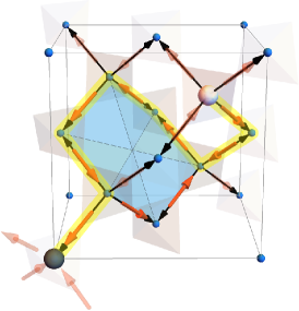
Figure 1: (a) The pyrochlore lattice of corner sharing tetrahedra, along with its parent diamond lattice. The diamond lattice is illustrated with light blue vertices at tetrahedron centers connected by thick black bonds. Each Ising spin (red arrow) sits at a pyrochlore site (black dots) at the midpoint of a diamond bond. The two states of the Ising variable $\sigma_{i}^{z}=\pm 1$ correspond to the two orientations of a classical spin-1/2 vector aligned along each bond, $\bm{S}_{i}=(\hbar/2)\sigma_{i}^{z}\hat{\bm{z}}_{i}$. Here, we show a portion of a 2-in-2-out ground state of the NNSI model, satisfying $Q_{t}=0$ on each tetrahedron. An open chain of five head-to-tail spins is highlighted (green). (b) Black arrowheads at the ends of each diamond bond in panels (b) and (c) indicate our convention for the quantization axes $\hat{\bm{z}}_{i}$, which point from the diamond $A$ to diamond $B$ sublattice. Flipping the open chain of spins creates a pair of opposite charges (Eq. 2) with $Q_{t}=+1$ (white) and $Q_{t}=-1$ (black) at the endpoints, connected by an electric flux string (yellow). The position of this string is only uniquely defined relative to the ground state in (a). One plaquette of the diamond lattice, a buckled hexagon, is shaded (blue). The six spins on the boundary of this plaquette form a closed chain (green). (c) Flipping the closed (green) chain of head-to-tail spins around the plaquette in (b) costs zero energy, and may be seen as moving the flux string (yellow) by effectively “reconfiguring the vacuum”. The minimal six-spin loop flips are precisely those generated in the ring exchange model of quantum spin ice [9].

II Preliminaries

To set the stage for this new spin model, we begin by briefly reviewing the physics of NNSI and its emergent gauge structure, which will serve as a crucial point of contrast throughout the rest of this paper. We then discuss its coarse-grained description to motivate an alternative mechanism for spin liquidity. In NNSI, $N_{\text{spin}}$ Ising spins are arranged on the sites of the pyrochlore lattice of corner-sharing tetrahedra, shown in Fig. 1(a). The centers of the tetrahedra (light blue spheres) form a bipartite diamond lattice, and each pyrochlore site (small black sphere) is located at the midpoint of a bond of this diamond lattice (thick black lines). The Ising spins (red arrows) are constrained to point in one of the two directions along the diamond bond, corresponding to the eigenstates of the spin-1/2 operator $\cramped{S^{z}_{i}\equiv\bm{S}_{i}\cdot\hat{\bm{z}}_{i}\equiv(\hbar/2)\sigma_{i}^{z}}$, where $\hat{\bm{z}}_{i}$ is the local quantization (cubic $[111]$ crystalline) axis at site $i$ and $\sigma_{i}^{z}$ is the Pauli-$z$ operator with eigenvalues $\pm 1$ [20]. We take the convention that the quantization axes point from the $A$ to $B$ diamond sublattices, represented in Fig. 1(b,c) as black arrowheads at the ends of the diamond bonds (Section A.1).

II.1 The Gauge Structure of NNSI

The NNSI Hamiltonian reads

$$H_{\text{NNSI}}=J\sum_{\langle ij\rangle}\sigma_{i}^{z}\sigma_{j}^{z},$$ (1)

where the sum is over nearest-neighbor sites of the pyrochlore lattice and $J>0$ sets the (antiferromagnetic) exchange energy scale. The essential physics of this model is exposed by defining a local lattice divergence [9, 3, 57] at each tetrahedron center (i.e. diamond vertex) $t$,

$$Q_{t}\equiv\frac{1}{2}(-1)^{t}(\sigma_{1}^{z}+\sigma_{2}^{z}+\sigma_{3}^{z}+\sigma_{4}^{z})_{t},$$ (2)

where $(-1)^{t}$ is positive (negative) on the $A$ ($B)$ diamond sublattices so that the divergence is positive, $\cramped{Q_{t}>0}$, when the majority of spins point “out” from the vertex $t$, such as illustrated in Fig. 1(b) on the tetrahedron carrying labels 1,2,3,4. By construction $Q_{t}$ takes values $0,\pm 1,\pm 2$, where the $+1$ ($-1$) configuration is illustrated in Fig. 1(b,c) on the tetrahedron carrying a white (black) sphere. In terms of $Q_{t}$, Eq. 1 takes the form

$$H_{\text{NNSI}}=E_{0}+2J\sum_{t}Q_{t}^{2},$$ (3)

where the sum is over all tetrahedra (diamond vertices) $t$, and $E_{0}=-JN_{\text{spin}}$ is the ground state energy. Ground states must satisfy the local zero-divergence constraint $Q_{t}=0$ everywhere (two spins “in” and two “out” of each tetrahedron, the “ice rules” [58]). Figure 1(a) shows a portion of such a 2-in-2-out ground state spin configuration, with spins denoted by red arrows. In these ground states, spins may be viewed as aligning head-to-tail to form closed strings [29, 27]. Flipping such a closed string of spins costs zero energy because it does not change $Q_{t}$ anywhere. The number of such degenerate ground states is exponentially large in the system size and, consequently, NNSI has an extensive entropy at zero temperature [59, 60, 27, 61, 58].

Minimal energy excitations are created by flipping a single spin, which produces a pair of defective tetrahedra with opposite divergence $Q_{t}=\pm 1$. More generally, flipping an open chain of head-to-tail spins, such as the five spins highlighted in green in Fig. 1(a), creates a pair of defective tetrahedra located at the two ends of the chain, as shown in Fig. 1(b). If we take the view that Eq. 2 is a Gauss law on the lattice [9, 24, 3], we may treat these excitations as fictional 0-dimensional point charges located on the diamond vertices at the centers of the tetrahedra (black and white spheres), which act as sources and sinks of the divergence of the spin configuration. These two charges appear to be connected by an open string of head-to-tail spins, shown in yellow in Fig. 1(b). The spin ice literature commonly describes these excitations as “monopole-antimonopole” pairs connected by “Dirac strings”, since they appear as sources of magnetization [28]. We shall utilize the dual perspective, more natural for the gauge theory description, viewing them as electric charge pairs connected by a 1-dimensional string of electric flux [9, 21].

Crucially, the positions of these closed and open electric strings are not observable. The decomposition of each spin configuration into a collection of strings is not unique [29]. The open (yellow) string shown in Fig. 1(b) is only defined relative to the ground state spin configuration in Fig. 1(a), and there are many possible strings one can find connecting a pair of charges. Having identified one such string, it can be deformed by flipping an “attached” closed loop of spins [29, 27]. This is demonstrated in Fig. 1(c), where the closed (green) string of six spins in Fig. 1(b) has been flipped, thereby deforming the open (yellow) string connecting the two charges. In a sense, the string between two charges is delocalized throughout a fluctuating vacuum of background ground state configurations, analogous to how the field of a point charge spreads over all space. This unobservability of the individual string positions characterizes the emergent gauge structure of the NNSI spin liquid as a string condensate [29, 27, 30].

II.2 A Different Kind of Spin Liquid

We now proceed to propose a new type of spin liquid lying beyond the description of charged quasiparticles connected by electric strings. To motivate its construction, let us recall that the long-wavelength description of the NNSI spin liquid is a Coulomb phase [3], described by a coarse-grained vector field $\bm{E}$ governed by a free energy of the form [31, 25, 26, 3, 29, 27]

$$F=\int\mathrm{d}^{3}r\;\big{(}\kappa|\bm{E}|^{2}+\xi^{2}|\nabla\cdot\bm{E}|^{2}\big{)},$$ (4)

where $\xi$ is a temperature-dependent lengthscale (with the density of defects $\rho\propto\xi^{-3}$ [3]). The quantity $\kappa$ is a stiffness parameter, which arises entropically (rather than energetically) from the fact that the spin length is bounded and thus the field strength cannot grow arbitrarily large [25, 3, 26, 29]. The Coulomb phase is obtained at zero temperature, at which point $\xi\to\infty$ and the divergence of $\bm{E}$ is fully suppressed [3, 27]. The correlation functions $\cramped{\langle E^{\alpha}(\bm{r})E^{\beta}(\bm{0})\rangle}$ then decay algebraically with the same $\cramped{1/r^{3}}$ form as a physical dipole-dipole interaction [31, 25, 26, 3, 27].

The vector field $\bm{E}$ can be decomposed into three components, known as the Helmholtz decomposition, with

$$\bm{E}=\nabla\phi+\nabla\times\bm{A}+\bm{E}_{0},$$ (5)

where $\phi$ is a scalar function, $\bm{A}$ is another vector field, and $\bm{E}_{0}$ satisfies Laplace’s equation. The three terms in Eq. 5 may be referred to as the irrotational (zero curl), rotational (zero divergence), and harmonic (both curl-free and divergence-free) components of $\bm{E}$, respectively. In the Coulomb phase, $\bm{E}$ has vanishing irrotational component ($\cramped{\nabla\phi=0}$), while the fluctuations of the rotational and harmonic degrees of freedom, each satisfying $\cramped{\nabla\cdot\bm{E}=0}$, are controlled by the Gaussian stiffness term in Eq. 4, $\cramped{\kappa|\bm{E}|^{2}}$. One may heuristically associate the irrotational component of $\bm{E}$ as sourced by the $\cramped{Q_{t}\neq 0}$ defects by a Gauss law, while the Gaussian-distributed rotational and harmonic component correspond to the degenerate ice manifold of closed-string configurations [57], with the harmonic component associated to strings that wind around the periodic boundaries [62].

At this juncture, with Eqs. 4 and 5 in mind, one may naturally wonder whether a microscopic lattice spin model analogous to NNSI exists for which the coarse-grained description takes the converse form,

$$\tilde{F}\sim\int\mathrm{d}^{3}r\;\big{(}\tilde{\kappa}|\bm{E}|^{2}+\tilde{\xi}^{2}|\nabla\times\bm{E}|^{2}\big{)}.$$ (6)

If such a model were to exist, it would naïvely have a degenerate ground state manifold consisting of all configurations with zero rotational component of the coarse-grained field $\bm{E}$. The excitations would be sources of the curl of $\bm{E}$ which, in Maxwell electrodynamics, would be a current-carrying wire—a string-like object—coupled by an emergent Ampere’s law, rather than the point-charge sources of the divergence of $\bm{E}$ in spin ice.

III The Spin Vorticity Model

To construct a microscopic spin model motivated by the coarse-grained form of Eq. 6, we consider reverse-engineering the spin ice Hamiltonian Eq. 3 by replacing the lattice divergence $Q_{t}$ with an appropriate definition of lattice curl, such that $\nabla\cdot\bm{E}$ in Eq. 4 is replaced with $\nabla\times\bm{E}$ in Eq. 6. To this end, we first define the vorticity, denoted $\omega_{p}$, on each hexagonal plaquette $p$ of the diamond lattice (buckled blue hexagon in Fig. 2) as the circulation of the spins around the plaquette boundary,

$$\omega_{p}=\frac{1}{2}(-1)^{p}(\sigma_{1}^{z}-\sigma_{2}^{z}+\sigma_{3}^{z}-\sigma_{4}^{z}+\sigma_{5}^{z}-\sigma_{6}^{z})_{p}.$$ (7)

Here, the spins are indexed sequentially around the perimeter of the plaquette as shown in Fig. 2. The alternating signs account for the alternating orientations of the quantization axes $\hat{\bm{z}}_{i}$ (small black arrowheads), so that $\omega_{p}$ is maximum when the six spins (red arrows) are oriented head-to-tail around the hexagon, as shown. The sign $(-1)^{p}$ depends on the chosen orientation of the plaquette (yellow plaquette normal arrow), so that $\omega_{p}$ is positive when the circulation has the same sense as the plaquette orientation by the right hand rule, analogous to the sign $(-1)^{t}$ in Eq. 2. By construction, $\omega_{p}$ takes values $0,\pm 1,\pm 2,\pm 3$, where the $+3$ configuration is illustrated in Fig. 2.

\begin{overpic}[width=346.89731pt]{Figures/hexagon.pdf} \put(33.0,48.0){$J_{3b}$} \put(67.0,48.0){$J_{2}$} \put(80.0,15.0){$J_{3a}$} \put(60.0,79.0){1} \put(25.0,77.0){2} \put(15.0,44.0){3} \put(38.0,18.0){4} \put(72.0,21.5){5} \put(82.0,53.0){6} \end{overpic}

Figure 2: A single hexagonal plaquette of the diamond lattice and corresponding hexagonal arrangement of tetrahedra in the pyrochlore lattice. The $A$ to $B$ orientation of the diamond edges is indicated with black arrowheads. A spin configuration (six red arrows) with vorticity $\omega_{p}=+3$ (Eq. 7) with respect to the orientation indicated by the yellow arrow is shown. Second neighbors are indicated by $J_{2}$ and the two types of third neighbors are indicated by $J_{3a}$ and $J_{3b}$.

We now define a new spin model, the spin vorticity model, by replacing $Q_{t}$ with $\omega_{p}$ in Eq. 3, i.e.

$$H_{\text{SV}}=\tilde{E}_{0}+J\sum_{p}\omega_{p}^{2},$$ (8)

where the sum is now over all hexagonal edge-sharing plaquettes $p$. Plugging Eq. 7 into Eq. 8 and expanding $\omega_{p}^{2}$, we obtain bilinear spin-spin interactions between all spins around each hexagon, i.e. first, second, and third-type-$b$ neighbors indicated in Fig. 2. The classical ground state energy $\cramped{\tilde{E}_{0}=-(3/2)JN_{\text{spin}}}$ has been added to cancel all single-site terms $\cramped{(\sigma_{i}^{z})^{2}=1}$. The spin vorticity Hamiltonian can then be written as

$$H_{\text{SV}}=-J\sum_{\mathclap{\langle ij\rangle}}\sigma_{i}^{z}\sigma_{j}^{z}+\frac{J}{2}\sum_{\langle ij\rangle_{\,\mathrlap{{2}}}}\sigma_{i}^{z}\sigma_{j}^{z}-\frac{J}{2}\sum_{\langle ij\rangle_{\,\mathrlap{3b}}}\sigma_{i}^{z}\sigma_{j}^{z}.$$ (9)

The reason the nearest-neighbor exchange energy is twice that of the further-neighbors is that every nearest-neighbor pair of spins belongs to two plaquettes (Section B.1). By construction, ground states of this Hamiltonian (with $\cramped{J>0}$) must satisfy the “zero-curl” condition $\cramped{\omega_{p}=0}$ on every plaquette, just as NNSI ground states obey the zero-divergence condition $\cramped{Q_{t}=0}$ at every diamond lattice vertex. Note that the nearest-neighbor exchange (first term in Eq. 9) is ferromagnetic with $J>0$, implying that this model is not adiabatically connected to NNSI. To demonstrate that this model indeed hosts a stable spin liquid, we next turn to analyzing its thermodynamic properties, before studying its emergent gauge structure.

III.1 SCGA Band Analysis

The self-consistent Gaussian approximation (SCGA) is a standard technique to study paramagnetic phases of spin models whose Hamiltonian takes the form (for Ising spins) $\cramped{H=(1/2)\sum_{ij}\sigma_{i}^{z}\mathcal{J}_{ij}\sigma_{i}^{z}}$, a method that has proven successful as a starting point for the analysis of spin liquids  [25, 31, 26, 63, 64, 65, 66]. Within the SCGA, the $\sigma_{i}^{z}$ are treated as continuous real variables and Lagrange multipliers $\lambda_{i}(\sigma_{i}^{z})^{2}$ are added to the Hamiltonian, subject to the average spin length constraints $\cramped{\langle(\sigma_{i}^{z})^{2}\rangle=1}$ (Section B.2). The resulting Gaussian theory is entirely controlled by the spectral decomposition of the interaction matrix $\mathcal{J}$, whose eigenvalues form four bands in reciprocal space for pyrochlore Ising models. Most classical spin liquids can be associated to a set of flat bands at the bottom of the spectrum of the interaction matrix, with the zero-temperature correlation matrix, $\cramped{\lim_{T\to 0}\langle\sigma_{i}^{z}\sigma_{j}^{z}\rangle}$, being proportional to the projector to the space spanned by the eigenvectors of the flat bands [8, 67].

For NNSI, $\mathcal{J}$ has two degenerate flat bands at the bottom of its spectrum [68, 31, 69, 26, 66] with a three-fold band touching point at the zone center, shown in Fig. 3(a) in the high-symmetry $(hhl)$ plane of reciprocal space (Section A.1). Performing a long-wavelength expansion of the interaction matrix for NNSI, one obtains an effective theory of the form Eq. 4 [26], revealing that the gapless band dispersing quadratically upwards from the band touching point corresponds to the irrotational component of the coarse-grained field $\bm{E}$, while the two dispersionless flat bands correspond to its rotational components (Section B.3).

\begin{overpic}[width=138.76157pt]{Figures/Bands_NNSI.pdf} \put(22.0,-6.0){$X$} \put(40.0,-8.0){$U$} \put(60.0,-3.0){$K$} \put(80.0,3.0){$L$} \put(-22.0,90.0){(a)} \put(-22.0,-24.0){(c)} \put(-22.0,-220.0){(e)} \put(114.0,90.0){(b)} \put(114.0,-24.0){(d)} \put(114.0,-220.0){(f)} \end{overpic}\begin{overpic}[width=156.10345pt]{Figures/Bands_Vorticity.pdf} \put(26.0,-6.0){$X$} \put(46.0,-8.0){$U$} \put(68.0,-2.0){$K$} \put(91.0,4.0){$L$} \end{overpic}

\begin{overpic}[width=433.62pt]{Figures/StructureFactor_SCGA_column.pdf} \end{overpic}

\begin{overpic}[width=164.77771pt]{Figures/pinchpoints_NNSI_3D.pdf} \end{overpic}\begin{overpic}[width=164.77771pt]{Figures/pinchpoints_Vorticity_3D.pdf} \end{overpic}

Figure 3: (a,b) The bands of the interaction matrix for (a) NNSI and (b) the spin vorticity model in the $(hhl)$ plane of reciprocal space. The flat rotational bands of NNSI (blue) correspond to the dispersive bands of the spin vorticity model and the dispersive irrotational bands of NNSI (red) correspond to the flat bands of the spin vorticity model. In both models the total bandwidth is $8J$. (c,d) The spin structure factor in the $(hhl)$ plane, computed in the SCGA for (c) NNSI and (d) the spin vorticity model at $T/J=0.01$, demonstrating that the correlations of these two models are “reciprocal”, with high and low intensity regions swapped, corresponding to swapping a suppressed divergence for a suppressed curl. (e,f) The pinch point at (002) for (e) NNSI and (f) the spin vorticity model, in the region indicted by the red circles in (c,d), showing that while the NNSI correlations are pinched along $\bm{q}$ (along $(00l)$), the vorticity correlations are pinched transverse to $\bm{q}$.

Figure 3(b) shows the bands of the interaction matrix for the spin vorticity Hamiltonian, Eq. 9. As in NNSI, there are two degenerate flat bands throughout the zone, indicative of a potential spin liquid ground state, and two degenerate dispersive bands and a fourfold band touching point at the zone center, already presaging significant contrast compared to NNSI. Performing a long-wavelength expansion of the spin vorticity model interaction matrix demonstrates that the two degenerate dispersing bands correspond to the two rotational components of the coarse-grained field $\bm{E}$ (Section B.3), while the flat bands correspond to the irrotational components. The long-wavelength form of the spin vorticity Hamiltonian Eq. 9 therefore has the desired form of the coarse-grained theory proposed in Eq. 6.

The relationship between the NNSI and spin vorticity models may be understood by observing first that the interaction matrices for these two models commute. Therefore they share eigenvectors, and one can continuously interpolate between them, changing the shape of the bands (the eigenvalues) but preserving the distinction of rotational and irrotational bands. Doing so (Fig. 14 in Section B.4) demonstrates that the flat rotational bands of NNSI continuously deform to the dispersive bands of the spin vorticity model (blue bands in Fig. 3(a,b)), while the dispersive irrotational bands of NNSI deform to the flat bands of the spin vorticity model (red bands). In other words, the rotational and irrotational modes exchange roles in the two models—the flat and dispersive bands of the spin vorticity model are irrotational and rotational, respectively. Thus, within the SCGA, the correlation matrices of the NNSI and spin vorticity models are projectors to complementary subspaces, and sum to the identity, except at $\bm{q}=\bm{0}$, where the two models share three eigenvectors at the threefold band touching point.

This “recipocality” of the spin ice and spin vorticity models is strikingly exposed in the low-temperature SCGA spin-spin correlation functions, encoded in the spin structure factor,

$$S(\bm{q})=\frac{1}{L^{3}}\sum_{ij}\langle\sigma_{i}^{z}\sigma_{j}^{z}\rangle\,e^{-i\bm{q}\cdot(\bm{r}_{j}-\bm{r}_{i})},$$ (10)

where $\bm{r}_{i}$ is the position of spin $i$ in the lattice and $L^{3}$ is the number of primitive FCC unit cells, assuming periodic boundary conditions. Figure 3(c) and (d) show $S(\bm{q})$ for NNSI and the spin vorticity model, respectively, computed using the SCGA. They appear “inverted” relative to each other: the pinch points in NNSI reflect the thermal extinction of the irrotational component of the coarse-grained field [3, 26], while the inverted intensity of the pinches of the spin vorticity model reflects the thermal depopulation of the rotational component of the field. This is most clearly seen in the three-dimensional structure of the pinch points, as shown in Fig. 3(e,f) for $\bm{q}=(002)$. For NNSI, the pinch is along $\bm{q}$, i.e. the longitudinal (irrotational) mode is suppressed, while for the spin vorticity model the pinch is orthogonal to $\bm{q}$, i.e. the transverse (rotational) modes are suppressed.

\begin{overpic}[width=86.72267pt]{Figures/SpecificHeat.pdf} \put(6.5,85.0){\footnotesize{Vorticity}} \put(8.0,25.0){\footnotesize{NNSI}} \put(44.0,31.0){\tiny{$T/J$}} \put(28.0,-6.0){$T/J$} \put(4.0,102.0){Specific Heat Per Spin} \put(29.0,-17.0){(a)} \put(105.5,-17.0){(b)} \put(163.5,-17.0){(c)} \put(220.0,-17.0){(d)} \put(289.0,-17.0){(e)} \end{overpic} \begin{overpic}[width=247.16656pt]{Figures/Structure_Factors_MC_SCGA.pdf} \put(16.0,55.0){\scriptsize{$T/J=2.0$}} \put(47.2,55.0){\scriptsize{$T/J=1.2$}} \put(78.6,55.0){\scriptsize{$T/J=0$}} \put(7.9,23.5){\footnotesize{SCGA}} \put(7.9,27.5){\footnotesize{MC}} \end{overpic} \begin{overpic}[width=86.72267pt]{Figures/Entropy.pdf} \put(11.0,102.0){Entropy per Spin} \put(35.0,68.0){\footnotesize{Vorticity}} \put(13.0,63.0){\footnotesize{NNSI}} \put(44.0,10.0){\tiny{$T/J$}} \put(28.0,-6.0){$T/J$} \end{overpic}

Figure 4: (a) The specific heat per spin as a function of temperature, $c(T)$, for the spin vorticity (blue) and NNSI (yellow) models measured in Monte Carlo simulations with $\cramped{L=32}$, with all results averaged over $10^{4}$ sample configurations per temperature. The spin vorticity model shows a sharp anomaly near $\cramped{T_{*}/J\approx 1.15}$ while NNSI only has a smooth crossover associated to the thermal depopulation of the tetrahedra that violate the two-in/two-out ice rules. (b,c,d) The $\cramped{L=32}$ spin structure factor $S(\bm{q})$ for the spin vorticity model at (b) $\cramped{T/J=2.0}$, (c) $\cramped{T/J=1.2}$ and (d) $\cramped{T/J=0}$, showing Monte Carlo data in the top panels and SCGA data below at a temperature chosen to match the diffuse intensity. The Monte Carlo correlations are consistent with the SCGA, but with the formation of weak Bragg peaks below $T_{*}$. The intensity of the peaks in (d) at (000), (111), and (002) are in the ratio $\cramped{(4:1:0)}$, respectively, consistent with all-in-all-out (AIAO) symmetry breaking (Section C.2). The color scale is linear from 0 to 8, matching Fig. 3(c,d), and logarithmic from 8 onward, to demonstrate that the Bragg peaks contain a negligible fraction of the total spectral weight. No interpolation or symmetrization has been applied to the data. Line cuts are provided in Section C.3. Note that at $T/J=0$, the pinch point intensity at (002) in the Monte Carlo simulation (top panel of Fig. 4(d)) is zero, while it is not in the SCGA (bottom panel of Fig. 4(d)), indicative of a lack of topological sector fluctuations using only local updates (Section IV.4.1). (e) The entropy per spin for the spin vorticity and NNSI models as a function of temperature, obtained by integrating $c(T)/T$, demonstrating that the spin vorticity model has an extensive ground state entropy remarkably close to that of NNSI.

III.2 Monte Carlo Analysis

The SCGA analysis indicates that the spin vorticity model may indeed host an extensive ground state and a novel spin liquid phase quite distinct from that of NNSI. While the SCGA is known to provide a good qualitative description of NNSI, it is only the first term in a large-$N$ expansion [70], where $N$ is the number of spin components. It remains to be demonstrated that the putative spin liquid phase implied by the flat bands of the interaction matrix survives in the Ising limit $N=1$, as it does in NNSI [31]. To do so, we perform classical Monte Carlo simulations of the spin vorticity Hamiltonian, Eq. 9, with $4L^{3}$ spins on an $\cramped{L\times L\times L}$ FCC lattice with periodic boundaries. We also simulate NNSI for comparison using a highly efficient cluster algorithm introduced in Ref. [71]. Details of our Monte Carlo procedures are provided in Section C.1.

In order to access low temperatures, we introduce a zero-energy cluster move for the spin vorticity model. In NNSI, a single spin flip in a ground state generates two tetrahedra with $\cramped{Q_{t}=\pm 1}$, and occurs with a probability exponentially suppressed by the Boltzmann factor $\exp(-4J/T)$. The ground state manifold of NNSI can instead be explored by flipping closed loops of spins discussed in Section II.1 [60, 72]. The minimal such “loop move” consists of flipping six spins around a hexagon as illustrated in Fig. 1(b,c). For the spin vorticity model, an analogous minimal cluster move is to flip four spins in an all-in or all-out tetrahedron, i.e. one with $Q_{t}=\pm 2$. We refer to this as a star move, since the four diamond bonds emanating from a single diamond vertex form a “star”. Each hexagonal plaquette of the diamond lattice (Fig. 2) shares either two spins with a given star or none. For each plaquette $p$ touching a given flippable star, the two spins contributing to $\omega_{p}$ are consecutive in Eq. 7 and satisfy $\cramped{\sigma_{1}^{z}=\sigma_{2}^{z}}$, i.e. both spins are in or both spins are out. They therefore contribute $\cramped{\sigma_{1}^{z}-\sigma_{2}^{z}=0}$ in Eq. 7, so that flipping them both does not change $\omega_{p}$ for that plaquette. Flipping all four spins in a star therefore does not change $\omega_{p}$ on any plaquette, and thus costs zero energy. We will discuss these zero energy star updates in more detail in the next section. We utilize both star moves and single spin flips in our Monte Carlo simulations of the spin vorticity model, with the primary results presented in Fig. 4.

III.3 Spin Liquid and Partial Long Range Order

Figure 4(a) shows the specific heat per spin, $c(T)$, as a function of temperature $T$ for both NNSI and the spin vorticity model. In NNSI, the specific heat displays a broad Schottky-like peak corresponding to the thermal depopulation of the minimal $\cramped{Q_{t}=\pm 1}$ excitations with energy cost of $2J$ [59, 60, 27, 73, 74]. In contrast, we observe a significant departure from this behavior in the spin vorticity model in the form of a sharp anomaly at $\cramped{T_{*}/J\sim 1.15}$, strongly suggestive of a finite-temperature phase transition that is not predicted by the SCGA. As we will see just below, however, this does not preclude the co-existence of a low-temperature classical spin liquid phase with extensive ground state entropy and critical correlations.

To investigate in more detail the potential spin liquidity and the nature of this specific heat anomaly, we track the evolution of the spin structure factor $S(\bm{q})$ (Eq. 10) with temperature, shown in Fig. 4(b-d) with Monte Carlo data in the top panels and the SCGA comparisons below. Starting with Fig. 4(b) at $\cramped{T/J=2.0}$, well above $T_{*}$, the spin-spin correlations are highly consistent with those computed within the SCGA, showing the formation of pinch point features (indicated by the white arrows) broadened at finite temperature. Moving to lower temperature, Fig. 4(c) shows $S(\bm{q})$ at $\cramped{T/J=1.2}$, just above $T_{*}\sim 1.15J$. The pinch points continue to sharpen, but we begin to see a deviation from the SCGA in the form of Lorentzian peaks (red) forming near the zone center ($\cramped{\bm{q}=\bm{0}}$).

Going below $T_{*}$, we can continue to thermalize all the way to zero temperature using the zero-energy star moves, shown in Fig. 4(d). Here we observe the formation of Bragg peaks characteristic of long-range order. This strongly suggests that the specific heat anomaly at $T_{*}$ is indeed a thermodynamic phase transition, with the pattern of peak intensities consistent with all-in-all-out (AIAO) symmetry breaking (Section C.2). However, the peak intensity is only about $0.4\%$ of the value that would be expected for a fully saturated AIAO order, $\cramped{S(\bm{0})=16L^{3}}$ (setting $\cramped{\sigma_{i}^{z}=1}$ in Eq. 10). Moreover, the diffuse “tails” beneath the Bragg peaks retain a Lorentzian intensity profile with finite width all the way to $\cramped{T=0}$ (see Section C.3 for line cuts of $S(\bm{q})$). Together, these observations imply that the phase transition at $T_{*}$ is not a transition to a “rigid” low-entropy phase. Rather, it is a “weak” symmetry breaking with the majority of the system maintaining predominant liquid-like correlations below $T_{*}$ all the way to zero temperature. This conclusion is evident in the diffuse intensity away from the Bragg peaks, which contains the vast majority of the spectral weight and remains highly consistent with the SCGA down to $T=0$. Thus the structure factor data implies that the low-temperature phase is a spin liquid, which coexists with a very weak long-range order.

Note that the possibility of a spin liquid coexisting with long-range order is not entirely novel. Indeed, the partial AIAO symmetry breaking we observe in the spin vorticity model is reminiscent of the phenomenon of “fragmentation” in spin ice, whereby a rigid crystalline arrangement of $Q_{t}=\pm 1$ charges is formed, but an extensive number of degrees of freedom continue to fluctuate as a spin liquid [75, 57]. We can rule out the presence of such a rigid charge crystal in the spin vorticity model, however, since such a crystal has magnetic Bragg peaks with $25\%$ of the intensity of full AIAO order [75], whereas those in Fig. 4(d) are only about $0.4\%$ of the fully saturated value.

\begin{overpic}[width=125.74689pt]{Figures/diamond_dual_interpenetrating2.pdf} \put(48.0,-13.0){(a)} \put(156.0,-13.0){(b)} \put(273.0,-13.0){(c)} \end{overpic} \begin{overpic}[width=125.74689pt]{Figures/diamond_dual_hexagons.pdf} \put(82.0,40.0){$\mathcal{A}$} \put(82.0,72.0){$\mathcal{B}$} \end{overpic}

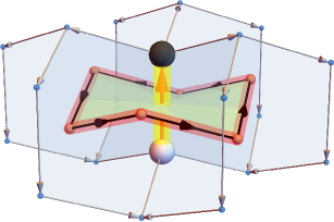
Figure 5: (a) A partial illustration of the relation between the direct diamond lattice—with blue vertices, white edges, and four blue plaquettes surrounding a three-dimensional volume—and the dual diamond lattice—with white vertices (spheres) and black edges shown. The dual diamond lattice has an associated along with a portion of the associated dual pyrochlore lattice (dark gray tetrahedra). (b) Illustration of the interpenetrating diamond and associated pyrochlore lattices, labeled $\mathcal{A}$ (direct) and $\mathcal{B}$ (dual), corresponding to the $\mathcal{A}_{2}\mathcal{B}_{2}\mathrm{O}_{7}$ oxide structure [18]. Each edge (plaquette) of the direct diamond lattice is dual to a plaquette (edge) of the dual diamond lattice. Each physical Ising spin (red arrow) is associated to an edge of the direct diamond lattice, and may equivalently be viewed as associated to a plaquette (green) of the dual diamond lattice. (c) The minimal excitation of the spin vorticity model is produced by flipping a single spin, which creates six defective plaquettes in the direct diamond lattice (light blue hexagons) with non-zero vorticity $\omega_{p}$ (indicated by thin gray arrows). The non-zero vorticity appears to be sourced by a loop of current (a string, red) “flowing” around the boundary of a dual (green) plaquette. Thus, in the spin vorticity model, each spin is fractionalized into a loop of current (red string) in the dual lattice, attached to a flux membrane (green). This contrasts with NNSI, where each spin is fractionalized into a pair of charges (black and white spheres) attached by a flux string (yellow). One may notice that these are the two fundamental representations of a dipole: a loop of current or a pair of charges.

III.4 Pinch Points and Ground State Entropy

It remains to assess if the pinch points become singular at $\cramped{T=0}$, in Fig. 4(d), reflecting the algebraic direct-space correlations of a Coulomb phase [3]. There are two symmetry-inequivalent pinch points, at the $\{002\}$ and $\{111\}$ positions. The width of the pinch points at the $\{111\}$ positions cannot be readily assessed, as they are hidden beneath the Bragg peaks (red) and appear broadened by the Lorentzian tails beneath the peak. On the other hand, the pinch point at the $\{002\}$ position is not covered by a Bragg peak, since this peak is forbidden for AIAO order (Section C.2). The shape of the (002) pinch point found in the Monte Carlo simulations, seen in Fig. 4(d), is highly consistent with the SCGA, which is most clearly seen from line cut comparisons (Section C.3). There is, however, one notable difference: in the Monte Carlo data, the intensity of the structure factor precisely at $\cramped{\bm{q}=(002)}$ is exactly zero. This can be seen by closely inspecting the top panel of Fig. 4(d) at the location marked by the two white arrows, comparing to the SCGA result at $(00\bar{2})$ in the bottom panel. In spin ice, the intensity at this point is related to the fluctuations of topological sectors [76]. We will return to clarify the origin of this “missing” intensity in Section IV.4.1 after developing an understanding of the emergent gauge structure of the ground state manifold.

To conclude our discussion of the thermodynamics of the spin vorticity model, we turn finally to the determination of the ground state degeneracy. Before doing so numerically, let us see how to construct a set of ground states exponentially large in the system size utilizing the zero-energy star moves (flipping four spins in an all-in or all-out tetrahedron). First, setting every $\sigma_{i}^{z}=+1$ or $-1$ in Eq. 7 demonstrates that the two AIAO configurations satisfy $\omega_{p}=0$ on every plaquette, and so are ground states of the spin vorticity model. Next, note that in these configurations every star is flippable and, in particular, all $L^{3}$ stars on a single diamond sublattice may be flipped independently. This generates $2^{L^{3}}$ ground states, and therefore gives a lower bound on the ground state entropy per spin of $\cramped{\ln(2)/4\approx 0.173k_{\text{B}}}$. Figure 4(e) shows the entropy per spin measured in Monte Carlo as a function of temperature for both NNSI and the spin vorticity model, which is computed by integrating the $\cramped{L=32}$ specific heat data from Fig. 4(a) (see Section C.4 for numerical integration details). We find that the zero-point entropy of the spin vorticity model is approximately $0.2055k_{\text{B}}$ per spin, remarkably close to that of NNSI [61]. We therefore conclude, based on the extensive ground state entropy, the diffuse paramagnetic correlations, and the pinched singularities in the structure factor, that the spin vorticity model with Ising ($\cramped{N=1}$) spins, Eq. 9, does indeed host a classical spin liquid ground state satisfying the local constraints $\omega_{p}=0$, albeit one that coexists with a weak AIAO symmetry breaking.

IV 2-Form Classical Spin Liquid

We now proceed to give a microscopic description of the ground state spin liquid, its fractionalized excitations, and its emergent gauge structure. To set the stage, recalling the discussion in Section II, let us quickly demonstrate how these properties can be deduced in NNSI, following from the local constraint $Q_{t}=0$. Starting from a ground state where the constraint holds, flipping a single spin creates the minimal excitation—a pair of equal and opposite charges on neighboring tetrahedra. In other words, each spin is fractionalized into a “dumbbell” of charges [28, 29]. Treating these dumbbells as “building blocks”, we imagine inserting them into the lattice one-by-one to construct a ground state. In order to ensure that $Q_{t}=0$ is satisfied, they must be placed in a head-to-tail fashion until they form a closed loop, so that all the charges cancel pairwise. This implies that every NNSI ground state can be decomposed (non-uniquely) into a collection of closed strings and, furthermore, that excitations (un-cancelled charges) appear at the ends of open strings. In this section, we will parallel this approach to expose the fractionalization and gauge structure of the spin vorticity model. In order to do so, we first need to introduce the dual diamond lattice, which will play a central role in the description of this physics and in the rest of this paper.

IV.1 Dual Diamond Lattice

The physical spin degrees of freedom are located on the sites of the pyrochlore lattice, and may equivalently be viewed as residing at the midpoints of the nearest-neighbor bonds of a diamond lattice. We call this the direct diamond lattice, illustrated in Fig. 1 with light blue vertices, thick black edges, and with a single plaquette (buckled hexagon) colored blue. Four of these plaquettes together form the surface of a three-dimensional volume of the direct diamond lattice, illustrated in Fig. 5(a), with the direct lattice edges now colored white for visualization convenience.

The dual lattice (or dual cell structure [77]) construction replaces each $p$-dimensional element of the direct lattice (vertex, edge, plaquette, volume) with a $\cramped{(d-p)}$-dimensional element of the dual lattice, where $d$ is the dimension of space. The dual lattice of the diamond lattice is another diamond lattice. It is illustrated in Fig. 5(a), with the dual vertices indicated by white spheres and the dual edges colored black. Note that the dual vertex ($\cramped{p=0}$, white) sits at the center of the direct lattice volume ($\cramped{p=3}$, blue), and each direct plaquette ($\cramped{p=2}$, blue) is pierced by a black dual edge ($\cramped{p=1}$, black).

Associated to the dual diamond lattice is a dual pyrochlore lattice, shown in Fig. 5(a) with dark gray tetrahedra, where each dual diamond vertex (white sphere) sits in the center of a dual pyrochlore tetrahedron. We note that in the common $\mathcal{A}$2$\mathcal{B}$2O7 pyrochlore oxide compounds, the direct pyrochlore lattice sites are occupied by the $\mathcal{A}$ ions and the dual pyrochlore sites are occupied by the $\mathcal{B}$ ions [18]. This is further illustrated in Fig. 5(b), which shows how the plaquettes of the dual diamond lattice (green) relate to the plaquettes of the direct diamond lattice (blue) and how the corresponding pyrochlore lattices (labeled $\mathcal{A}$ and $\mathcal{B}$) interpenetrate one another. Each edge of the dual diamond lattice (black line) pierces a plaquette of the direct diamond lattice (blue hexagon) and each edge of the direct lattice (gray line) pierces a dual plaquette (green hexagon), so that the plaquettes “link” each other, as shown. We can now make a key observation: each microscopic Ising spin (red arrow), located at a site of the direct ($\mathcal{A}$) pyrochlore lattice may be viewed either as a 1-dimensional flux along a direct diamond lattice edge, as in NNSI, or as a 2-dimensional flux through a dual lattice plaquette. We will see that the latter perspective is required to understand the emergent gauge structure of the spin vorticity model.

\begin{overpic}[width=130.08731pt]{Figures/flux_cancellation.pdf} \put(41.0,-8.0){(a)} \put(160.0,-8.0){(b)} \put(277.0,-8.0){(c)} \end{overpic}

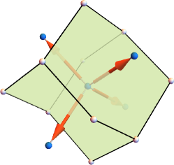
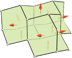
Figure 6: (a) Ground states are formed by arranging spins in such a way that all of the “currents” running around the dual plaquettes cancel. This is achieved when the spins form a closed, oriented surface. The smallest such closed membrane is the one shown in (b), corresponding to a “star” of the direct diamond lattice. A larger membrane with ten spins is shown in (c). Flipping a collection of spins forming such a closed membrane costs zero energy, directly analogous to the flipping of closed loops in NNSI.

IV.2 String Fractionalization

Starting from any ground state satisfying $\omega_{p}=0$ on every direct plaquette (Fig. 2), consider flipping a single spin. After the flip, six direct plaquettes have non-zero vorticity, $\omega_{p}=\pm 1$, illustrated in Fig. 5(c) by the six lightly shaded blue hexagons, costing a total energy $6J$ (one $J$ for each hexagon coming from Eq. 8). Thus a single spin flip is at first glance fractionalized into six excitations. However, interpreting the vorticity $\omega_{p}$ as the lattice curl on direct plaquette $p$ (i.e. the circulation around the boundary of the plaquette), we may imagine that it is sourced by a “current” via an emergent Ampere’s law, where the current is “flowing” along the 1-dimensional dual edge piercing direct plaquette $p$. Together, the six defect plaquettes carrying $\omega_{p}\neq 0$ after the single spin flip then appear to be sourced by a closed loop of current running around the boundary of the green dual plaquette, indicated in Fig. 5(c) by a red string, with black arrowheads indicating the direction of flow. Note that, as we will see in more detail in Section IV.5, these string objects are better thought of as string charges rather than currents, i.e. there is really nothing flowing along the string. We utilize the current description only to draw analogy with the intuition of Maxwell electrodynamics.

We conclude that in the spin liquid of the spin vorticity model, spins are fractionalized into closed strings. These may be viewed as fictional currents “flowing” along the edges of the dual lattice, acting as sources of the spin vorticity via an emergent Ampere’s law. The spins may be thus be viewed as fluxes through the 2-dimensional dual plaquettes, shown in green in Fig. 5(b,c), attached to oriented strings on their boundaries. This contrasts with the fractionalization of NNSI, where each spin acts as a short string of electric flux along a direct diamond edge, attached to a pair (i.e. dumbbell) of opposite electric charges, which act as (fictional) sources of divergence of the spin configurations [28]. These two perspectives are juxtaposed in Fig. 5(c): The spin ice dumbbell is shown as a pair of charges (black and white) attached to the ends of a 1-dimensional flux string along a direct lattice edge (yellow); the equivalent fractionalized object in the spin vorticity is an oriented string on the boundary of a dual plaquette (red), attached to a 2-dimensional flux membrane (green). These two pictures are naturally complementary—they correspond to the two classical representations of a dipole: either a pair of opposite charges, or a loop of current. In NNSI, each spin (dipole) is fractionalized in the former way, while in the spin vorticity model they fractionalize in the latter way.

\begin{overpic}[width=121.41306pt]{Figures/membrane_string_tiling3.pdf} \put(45.0,-25.0){(a)} \put(165.0,-25.0){(b)} \put(300.0,-25.0){(c)} \end{overpic}

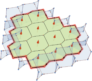
Figure 7: (a) Single spin flips create a small string-loop excitation in the dual lattice attached to a two-dimensional flux (Fig. 5(c)), and general excitations are created by flipping a collection of spins which tile an open surface, such that the strings (red) cancel in the interior of the surface, leaving a single string circulating around the boundary. (b) A string excitation created by flipping twelve spins. Each direct plaquette (blue) pierced by the string carries non-zero vorticity, $\omega_{p}\neq 0$. The energy of the string is $J$ times the number of defect plaquettes, i.e. the length of the string. In the direct lattice, there is a net circulation of the spins along any closed contour that links the string(Appendix D). (c) The membrane attached to a given string is not observable, it is only well-defined relative to a fixed ground state configuration, just as is the case for the strings in spin ice (see Fig. 1). Here we show two possible membranes attached to the same string (spins are not shown for clarity). Flipping one or the other differs by flipping the closed membrane formed by gluing them together.

IV.3 Ground State Manifold: Topological Membrane Condensate

In order to construct a ground state, we imagine placing the spins into the lattice one by one, each thought of according to Fig. 5(c) as a 2-dimensional flux through a dual plaquette with a 1-dimensional current running around around its boundary. To form a ground state, these plaquettes must be placed so that all of the currents along their boundary edges cancel pairwise, meaning that there are no direct plaquettes with $\omega_{p}\neq 0$. This is achieved when they are arranged to form a closed oriented surface in the dual lattice, meaning that the total flux through the surface is maximally polarized. The minimal such arrangement is achieved with four plaquettes, illustrated in Fig. 6(a). This implies that every ground state of the spin vorticity model is decomposable, non-uniquely, into a collection of closed, oriented membranes. We conclude that the spin vorticity model spin liquid ground state may be described as a membrane condensate, generalizing the string condensate of NNSI.

The smallest such membrane consists of four plaquettes shown in Fig. 6(b), with the four spins pointing all-out or all-in, and a larger membrane consisting of ten spins is shown in Fig. 6(c). Flipping all of the spins forming one of these closed membranes, no matter its size or shape, produces another configuration with the same energy, analogous to flipping closed loops of spins in spin ice [78, 60]. This is because the circulation around any loop of direct-lattice edges piercing the membrane is unchanged by this collective spin flip—such a loop passes “in” and “out” of the membrane an equal number of times, and so flipping a membrane does not change $\omega_{p}$ anywhere (Appendix D). Notice that the minimal membrane (green) shown in Fig. 6(b) is precisely the “star” of four spins surrounding a direct diamond lattice vertex, corresponding to an all-in or all-out tetrahedron of the pyrochlore lattice. Thus the star moves, described in Section III.2 and used to generate the Monte Carlo results in Fig. 4, are precisely the smallest possible membrane flipping update.

Note that flipping any membrane that is the surface of a 3-dimensional volume is equivalent to applying a star move to every minimal membrane (i.e. every star or tetrahedron) contained inside the volume. Therefore, using only the minimal star move updates in our Markov chain Monte Carlo is equivalent, after a sufficient number of such updates, to finding and flipping large membranes which bound a three-dimensional volume. On the other hand, there are topologically non-trivial surfaces which wind around the periodic boundaries (or around any hole), which are not the boundary of any volume. Flipping such a non-contractible membrane is never equivalent to any sequence of local flips of topologically trivial membranes. The ground state manifold is therefore divided into topological sectors, which are connected by flipping non-contractible membranes. This parallels the topological sectors of NNSI, which are connected by flipping non-contractible strings [63, 72]. Notice that a star move (flipping an all-in to all-out tetrahedron or vice versa) does not change the net magnetization, from which it follows that flipping a contractible membrane conserves the net magnetization of the system, $\sum_{i}\bm{S}_{i}$. On the other hand, flipping a flat surface of all-down spins winding around the periodic boundaries to all-up clearly changes the magnetization (see Section C.5 for further details). We conclude that the topological sectors differ by their net magnetization.

Why we obtain membranes from a zero-curl condition can be understood via the Helholtz-Hodge decomposition, Eq. 5. Any vector field configuration with zero rotational component can be written as a gradient of a scalar function (neglecting boundaries), such that the vector field always points orthogonal to the equipotential surfaces. This implies that the ground states of the spin vorticity model in the zero-magnetization sector may be expressed as an integer-valued function $\phi$ on the diamond lattice vertices, whose value $\phi_{t}$ increases or decreases by 1 across each diamond link, such that the spin on the edge connecting $t$ to $t^{\prime}$ has value $\sigma^{z}_{tt^{\prime}}=\phi_{t^{\prime}}-\phi_{t}$. Thus each topologically-trivial ground state configuration can be decomposed into a collection of equipotential surfaces in the dual diamond lattice, along which the spins all point in the same direction, such as illustrated in Fig. 6(b,c). This may be viewed as a 3D version of a height-representation [79, 3], with $\phi$ the “height” field. Ground states in a non-trivial topological sector configuration (one with non-zero net magnetization) must be expressed as a combination of $\phi_{t}$ plus an extra piece, the harmonic component of the decomposition. This may be done by fixing the spins on a set of non-contractible membranes, which fixes a topological sector, effectively dividing the system into a set of contractible domains with spins fixed along their boundaries, within each of which the remaining spins can be represented as the gradient of $\phi$. The topological sector is determined by the winding number $w[C]:=\sum_{i\in C}(-1)^{i}S_{i}^{z}$ along non-contractible loops $C$ which link one of the three handles of the torus, where $(-1)^{i}$ alternates along the loop. These winding numbers can only change in a ground state by flipping a non-contractible membrane of spins, but are ill defined in the presence of excitations. The analogous winding number in spin ice are the net flux through three planes of the lattice [9]. See Appendix D for further details.

In summary, the ground states of the spin vorticity model can be decomposed into a collection of closed, oriented membranes, directly analogous to how ground states of spin ice can be decomposed into a collection of closed, oriented strings [72]. Such a decomposition is not unique, thus characterizing this phase as a condensate of membranes. Flipping one of these closed membranes costs zero energy because it does not change the vorticity $\omega_{p}$ on any plaquette, analogous to how flipping a closed loop in spin ice does not change the charge $Q_{t}$ on any tetrahedron [78, 60]. The ground state manifold is divided into topological sectors, differing by net magnetization and connected by flipping of non-contractible membranes.

\begin{overpic}[width=433.62pt]{Figures/winding.pdf} \put(47.0,30.0){(a)} \put(47.0,-5.0){(b)} \end{overpic}

Figure 8: (a) In spin ice, the topological sector can fluctuate by creation of a pair of charges, running one around the periodic boundaries, and re-annihilating the pair, equivalent to flipping a non-contractible string. (b) In the spin vorticity model, the equivalent mechanism is to nucleate a single string, grow it to the size of the system, then re-contract it around the periodic boundaries until it annihilates itself, equivalent to flipping a non-contractible membrane.

IV.4 Excitations: String Charges

The minimal excitation, created by flipping a single spin, is a small string (or “current loop”) in the dual diamond lattice, shown in Fig. 5(c). More generally, excitations are created by flipping a collection of spins forming an open surface, such as shown in Fig. 7(a) with three spins. The string segments in the interior of the surface cancel each other, while the uncancelled edges on the boundary of the surface carry a longer 1-dimensional string excitation, attached to a two-dimensional flux membrane in the interior of the surface. Figure 7(b) shows a string excitation created by flipping twelve spins forming a flat open membrane. Each direct plaquette (blue) pierced by the string carries a non-zero vorticity, $\omega_{p}$. The net circulation around any loop in the direct lattice which links the string in the dual lattice is non-zero (Appendix D). There is no unique open membrane attached to a given string excitation, just as the closed membranes are not uniquely defined. Having identified an open membrane attached to a string, it may be deformed by flipping a closed membrane that touches it. This parallels how flipping closed loops in NNSI deforms the position of the string connecting a pair of charges, shown in Fig. 1(b,c). Figure 7(c) depicts two different membranes attached to the same string. Given a spin configuration, there are many possible membranes one can find, of arbitrary size and shape, connected to the same string.

These extended string excitations cost energy proportional to their length, specifically $J$ times the number of direct plaquettes pierced by the string, which have $\omega_{p}=\pm 1$ in the dilute limit. For a plaquette pierced by two overlapping strings with the same local orientation, so that $\omega_{p}=\pm 2$, the energy cost on that plaquette is $4J$. This is higher than the $2J$ energy cost of two separate single-defect plaquettes, meaning there is an extra energy cost associated to parallel strings which overlap. Thus, strings with the same local orientation energetically repel each other, and may be considered to have the same charge. On the other hand, strings with opposite local orientation may fuse, annihilating along their overlap and thus lowering the total energy by minimizing the total string length. Thus there is an energetic attraction between anti-parallel strings, and they may be considered to have opposite charges. This is quite distinct from NNSI, where the point charge excitations come in two species, either positive or negative. By contrast, the strings of the spin vorticity model do not come in two charge species, instead they come with an orientation, and the relative charge of two local string segments is determined by their relative orientations. A pair of strings may be locally parallel and thus repelling in one place, but anti-parallel and thus attracting in another, and indeed a single string can interact with itself. Although these are only local contact interactions, it would be interesting to study in more detail the entropic interaction of these strings, which yields a $1/r$ Coulomb potential between charges in NNSI [28, 29], as well as how further-neighbor interactions can be tuned to control the interaction potential between strings [80, 81].

IV.4.1 Topological Sector Ergodicity

The fact that the energy of a string scales with its length highlights a crucial qualitative distinction between the spin vorticity model and spin ice. In spin ice, the topological sector can be changed by nucleating a pair of charges out of a ground state, costing a total energy $4J$, moving one around the handle of the torus, and annihilating them, costing no additional energy. This process is illustrated in Fig. 8(a), which effectively inserts a string of flux around the periodic boundaries. In the spin vorticity model on the other hand, the analogous operation is to nucleate a single string, grow it to the size of the torus until it wraps around the periodic boundaries, then re-contract it to annihilate itself, as illustrated in Fig. 8(b). However, a string the size of the torus costs energy proportional to the linear size of the system, and is thus forbidden in the thermodynamic limit. This observation implies that the spin vorticity model loses topological sector ergodicity with only local dynamics at sufficiently low temperatures, when the density of string defects and their average length falls below some threshold.

This loss of topological sector ergodicity explains naturally why the pinch point intensity of the structure factor measured in the Monte Carlo simulations, shown in Fig. 4(d), is exactly zero at the $(002)$ point at $T=0$. Since our algorithm utilizes only local updates, the lack of topological sector fluctuations at low temperatures means that the net magnetization freezes, resulting in an extinction of the zone-center pinch point intensities (see Section C.5 for further details). It would be interesting to investigate whether there is a critical temperature associated with a percolation threshold for the strings, i.e. a critical average density and string length at which the strings form a percolating network, and whether it is related to the thermodynamic transition observed in the Monte Carlo simulations.

Figure 9: The classical spin liquid Coulomb phase of the spin vorticity model is described by 2-form electrodynamics, with charged string excitations interacting with a 2-form gauge field. This has properties not shared by the emergent 1-form Coulomb phase of NNSI, where charges are always created in positive-negative pairs connected by a string of electric flux (Fig. 1). Each string (red) of the spin vorticity model carries local charge but is globally charge-neutral, which is reflected in the fact that many strings may be connected by a single flux membrane (green). Here we show three such strings.

IV.5 2-Form Electrodynamics & Coulomb Spin Liquid

Recall that we initially set out to invert the rotational-irrotational description of the Coulomb phase of spin ice, by replacing the divergence in Eq. 4 with a curl in Eq. 6. What has been achieved in the process is to raise the dimension of the microscopic charged particles and flux strings of NNSI by one, to charged strings and flux membranes, respectively. Whereas NNSI realizes a Coulomb phase where charged particles couple to an electric field whose field lines are strings, the spin vorticity model realizes a generalized Coulomb phase, where charged strings couple to an electric field whose “field lines” are membranes.

A natural language to describe such “generalized” Coulomb phases can be found in the formalism of so-called “$p$-form electrodynamics”, developed by Henneaux and Teitelboim [47]. This is a natural generalization of Maxwell electrodynamics to $(p-1)$-dimensional electrically charged objects interacting with a rank-$p$ antisymmetric tensor electric field, called a $p$-form. In differential geometry, $p$-forms are the natural objects which can be sensibly integrated over a $p$-dimensional surface. A brief semi-technical introduction to $p$-form electrodynamics is provided in Appendix G. The case $p=1$ describes traditional Maxwell electrodynamics of point charges interacting with a 1-form (vector) electric field, which describes the emergent point charges attached to 1-dimensional electric flux lines in spin ice. The case $p=2$ describes string charges interacting with a 2-form electric field, and is the appropriate description for the emergent generalized Coulomb phase of the spin vorticity model described in this section, which hosts charged string excitations attached to 2-dimensional electric flux membranes.

A hallmark feature of $p$-form electrodynamics is that the charged excitations for $p>1$ are charge-neutral, i.e. extended charged objects are their own “anti-particles” [47]. We can clearly see this in the spin vorticity model, because flipping a single spin creates only one string excitation, rather than a pair of opposite-charged excitations. Correspondingly, an isolated string can shrink and vanish into the vacuum without having to annihilate with another string. Furthermore, the 2-dimensional electric flux membranes can connect a single charged string to itself, such as depicted in Fig. 7(b). As we discussed in Section IV.4, the charge is defined by the local orientation of the string, such that locally parallel string segments may be considered to have the same charge while locally anti-parallel string segments may be considered to have opposite charge. This behavior contrasts with the 1-form Coulomb physics of spin ice, where point charges can only ever be created in positive-negative pairs at the ends of an open string, i.e connected by a line of electric flux. In the spin vorticity model, since a membrane may have an arbitrary number of boundary components (holes), a single electric membrane may connect an arbitrary number of charged strings together, such as the three strings connected by a single membrane shown in Fig. 9.

We conclude that the spin vorticity model realizes a classical 2-form spin liquid, i.e. an emergent 2-form Coulomb phase. To the best of our knowledge, this is the first example of a lattice spin model realizing such a phase. We note that it is not strictly necessary to use the pyrochlore lattice to define a spin vorticity model, since the vorticity, Eq. 7, can be defined for various line graph lattices in three dimensions [3]. Our main motivation for having used the pyrochlore lattice is to establish a direct juxtaposition with the physics of NNSI, for which the emergent (1-form) electrodynamics has been extensively studied, both technically and experimentally in the past twenty-five years.

V 2-Form U(1) Quantum Spin Liquids

Up to this point we have considered the classical spin vorticity model defined by the Hamiltonian Eq. 9, and demonstrated that it realizes an emergent 2-form Coulomb phase, i.e. a 2-form classical spin liquid. Specifically, in the language of 2-form electrodynamics [47], the membranes are 2-form electric fluxes, which are attached to emergent, fractionalized, charged string excitations. This classical model is interesting in its own right, and could potentially be realized at finite temperatures in a materials setting. We now move to study the effects of perturbing it with weak quantum exchange interactions, which can drive tunneling between the classical ground states. Such considerations raise the possibility for a novel class of quantum critical phases: 2-form U(1) quantum spin liquids.

As a minimal definition of what such a liquid is, we search for a quantum model whose ground state is a coherent superposition of the classical ground states of the classical spin vorticity model. In this section, we demonstrate in broad strokes how to construct such a “quantum spin vorticity” (QSV) model. We will show that the resulting model maps at second order in perturbation theory to a 2-form U(1) lattice gauge theory, which can be tuned with a four-spin interaction to a point where the desired superposition ground state is achieved. This serves as a proof of concept for the 2-form U(1) QSL, thus laying the groundwork for deeper study of such higher-form quantum spin liquids. Building on this, we demonstrate how the string excitations may be treated within the lattice gauge theory framework, and end with a discussion of the stability of 2-form U(1) QSL phases, placing these phases within the context of well-known U(1) superfluid and spin liquid phases. In the remainder of this section, we switch to quantum spin-1/2 operators $S^{z}_{i}=(\hbar/2)\sigma^{z}_{i}$, along with the local transverse spin components $S_{i}^{x}$ and $S_{i}^{y}$ defined with the standard symmetry convention [20] (Section A.1), and work in units with $\hbar=1$.

V.1 Quantum Membrane Exchange Dynamics

In addition to the Ising $\cramped{S_{i}^{z}S_{j}^{z}}$ terms appearing in the classical Hamiltonian, there are generically three other possible two-spin interactions allowed by symmetry at nearest-neighbor on the pyrochlore lattice, which have the form $\cramped{S_{i}^{\pm}S_{j}^{\mp}}$, $\cramped{S_{i}^{z}S_{j}^{\pm}}$, or $\cramped{S_{i}^{\pm}S_{j}^{\pm}}$, where $\cramped{S^{\pm}=S^{x}\pm iS^{y}}$ [20]. Treating these terms within degenerate perturbation theory generates operators acting on up to $2n$ spins at order $n$. We are then interested in the lowest order operators that have matrix elements connecting one classical ground state to another. When perturbing the NNSI model, the most important term is the $\cramped{S_{i}^{\pm}S_{j}^{\mp}}$, which at third order generates the effective ring exchange model of quantum spin ice (QSI) [9]. The ring exchange term flips fully-polarized loops of six spins, as illustrated in Fig. 1(b,c), generating quantum dynamics within the classical ground state manifold and driving the quantum spin liquidity. In this section we consider the effects of quantum perturbations to the classical spin vorticity model.

We consider now perturbing the classical spin vorticity model with the three above-mentioned terms. In this case, as we will see, the important leading-order effect is generated by the $\cramped{S_{i}^{\pm}S_{j}^{\pm}}$ term. We thus consider a minimal “quantum spin vorticity model” with Hamiltonian given by

$$H_{\text{QSV}}=H_{\text{SV}}+J_{\pm\pm}\sum_{\langle ij\rangle}(S_{i}^{+}S_{j}^{+}+S_{i}^{-}S_{j}^{-}).$$ (11)

At second order in degenerate perturbation theory, one obtains quantum tunneling between two classical ground states, via the flipping of four spins shown in Fig. 10. This process defines an effective Hamiltonian given by

$$H_{\text{ME}} =J_{\text{mem}}\sum_{t}(S_{1}^{-}S_{2}^{-}S_{3}^{-}S_{4}^{-}+S_{1}^{+}S_{2}^{+}S_{3}^{+}S_{4}^{+})_{t}\,,$$

$$\equiv J_{\text{mem}}\sum_{\vbox{\hbox{\includegraphics[height=8.67204pt]{Figures/volume_tiny.pdf}}}}\left(\,\,\ket{\vbox{\hbox{\includegraphics[height=20.2355pt]{Figures/mem_in.pdf}}}}\bra{\vbox{\hbox{\includegraphics[height=20.2355pt]{Figures/mem_out.pdf}}}}+\ket{\vbox{\hbox{\includegraphics[height=20.2355pt]{Figures/mem_out.pdf}}}}\bra{\vbox{\hbox{\includegraphics[height=20.2355pt]{Figures/mem_in.pdf}}}}\,\,\right),$$ (12)

where $\cramped{J_{\text{mem}}\propto J_{\pm\pm}^{2}/J>0}$, and the numbering is over the four spins in a tetrahedron (see Fig. 1(b)). In the second line of Eq. (12), we have pictorially represented the operator in terms of Fig. 6(b), as flipping a single minimal membrane from an all-out to an all-in configuration or vice versa. In other words, this operator precisely implements the star move, thereby generating local quantum dynamics for the membranes. Thus we call the effective Hamiltonian in Eq. 12 a membrane exchange (ME) model, directly analogous to the ring exchange model of QSI [9, 34, 21].

\begin{overpic}[width=433.62pt]{Figures/membrane_exchange_generation_SpmSpm.pdf} \put(31.0,29.0){$S_{i}^{\pm}S_{j}^{\pm}$} \put(64.0,-2.0){$S_{k}^{\pm}S_{l}^{\pm}$} \end{overpic}

Figure 10: Applying $S_{i}^{\pm}S_{j}^{\pm}$ from Eq. 11 twice to a classical ground state creates an intermediate excited state with a string costing energy $8J$, then annihilates it to generate another classical ground state with four spins flipped, thus generating membrane exchange.

The membrane exchange model gives an intuitive picture for the quantum dynamics of the proposed 2-form quantum spin liquid phase, but we can go further. By adding to the Hamiltonian a generalization of the Rokhsar-Kivelson (RK) term [9, 82, 21, 83], which acts as a chemical potential for flippable membranes, we can tune the model to an exactly-solvable point. The RK term includes interactions of four spins on each tetrahedron, given by

$$H_{\text{RK}} =V\sum_{t}\left[\sum_{\eta=\pm 1}\prod_{i\in t}\left(\frac{1}{2}+\eta S_{i}^{z}\right)\right]\,,$$

$$\equiv V\sum_{\vbox{\hbox{\includegraphics[height=8.67204pt]{Figures/volume_tiny.pdf}}}}\left(\,\,\ket{\vbox{\hbox{\includegraphics[height=20.2355pt]{Figures/mem_in.pdf}}}}\bra{\vbox{\hbox{\includegraphics[height=20.2355pt]{Figures/mem_in.pdf}}}}+\ket{\vbox{\hbox{\includegraphics[height=20.2355pt]{Figures/mem_out.pdf}}}}\bra{\vbox{\hbox{\includegraphics[height=20.2355pt]{Figures/mem_out.pdf}}}}\,\,\right),$$ (13)

which counts the number of flippable stars (i.e. minimal closed membranes), with $V>0$. The RK operator is diagonal in the $S^{z}$ basis, with positive entries $V$ times the number of flippable stars, while the membrane exchange term Eq. 12 is off-diagonal with positive matrix elements $J_{\text{mem}}$. The sign of $J_{\text{mem}}$ can be changed via a unitary transformation, by applying a $\pi$ rotation about the local $z$-axis to every spin on a single pyrochlore sublattice (Section A.1), which changes $S_{i}^{\pm}\to-S_{i}^{\pm}$ in Eq. 12 for exactly one spin on every tetrahedron. This makes all of the off-diagonal matrix elements of the Hamiltonian non-positive. Tuning $V\to J_{\text{mem}}$, the Hamiltonian can then be written as a sum of projectors

$$H_{\text{RK}-\text{ME}}=V\sum_{\vbox{\hbox{\includegraphics[height=8.67204pt]{Figures/volume_tiny.pdf}}}}\left(\,\ket{\vbox{\hbox{\includegraphics[height=20.2355pt]{Figures/mem_in.pdf}}}}-\ket{\vbox{\hbox{\includegraphics[height=20.2355pt]{Figures/mem_out.pdf}}}}\,\right)\,\left(\,\bra{\vbox{\hbox{\includegraphics[height=20.2355pt]{Figures/mem_in.pdf}}}}-\bra{\vbox{\hbox{\includegraphics[height=20.2355pt]{Figures/mem_out.pdf}}}}\,\right).$$ (14)

Since this Hamiltonian is a projector, with eigenvalues $0$ or $V$, any state it annihilates is a ground state. The ground state is then an equal-weight superposition of every classical closed-membrane ground state [82, 9, 83],

$$\ket{0}_{\text{RK}}=\mathcal{P}\,\prod_{i}\,\frac{1}{\sqrt{2}}\left(\ket{S_{i}^{z}=+\tfrac{1}{2}}+\ket{S_{i}^{z}=-\tfrac{1}{2}}\right),$$ (15)

where $\mathcal{P}$ is the projector to the classical ground state manifold of closed-membrane configurations, and the state it acts on is an equal-weight superposition of all classical configurations . This demonstrates the existence of a fine-tuned point whose quantum ground state may be described as a 2-form QSL, i.e. a massive coherent superposition of the classical 2-form spin liquid ground states. Note that the RK point is generically unstable to the addition of relevant perturbations—in the ring exchange model of QSI it corresponds to the boundary between the QSL and an ordered phase [9, 34, 84, 21]. We take the existence of the RK point in the membrane exchange model as a proof of concept that a Hamiltonian with a 2-form QSL ground state exists, leaving an in-depth analytical and numerical study for future work. The issue of the stability of the putative QSL ground state away from the fined-tuned RK point is discussed further in Section V.5.

In the next section we will discuss how to map the membrane exchange model to a 2-form lattice gauge theory but, before moving on, the existence of an RK point naturally begs the question of whether 2-form spin liquids, either quantum or classical, can be described using dimer models, which play an important role in our understanding of strongly correlated liquid phases [82, 85, 86, 79, 83, 21]. Spin ice can be mapped to a dimer model by replacing the two Ising spin states, $\sigma_{i}^{z}=\pm 1$, with the presence or absence of a dimer on the corresponding diamond lattice edge, such that the constraint $Q_{t}=0$ translates to having two dimers touching at every diamond vertex, such that every spin ice ground state corresponds to a dimer loop covering of the diamond lattice [21], with similar loop-gas descriptions widely utilized for studying Coulomb phases [83, 3]. Naïvely applying this map to the spin vorticity model, the constraint $\omega_{p}$ translates to a non-local constraint on dimers sitting on the edges of the direct lattice hexagonal plaquettes. A more natural description would involve replacing 1-dimensional dimers by 2-dimensional hard plaquettes on the dual lattice, which then touch at each dual edge. One then seeks a basis for which the constraint $\cramped{\omega_{p}=0}$ translates to the constraint that exactly three hard plaquettes touch at each dual edge. However, we show in Appendix E that no such basis exists. Further work is required to determine if either dimer or hard-plaquette [87] models with local constraints can faithfully describe 2-form spin liquids.

V.2 2-Form U(1) Lattice Gauge Theory

We now demonstrate how to map the membrane-exchange Hamiltonian, Eq. 12, to a lattice gauge theory, in parallel to the ring exchange model of QSI [9]. The key difference is that the membrane exchange model maps to a 2-form U(1) gauge theory, while the ring exchange model maps to a conventional 1-form gauge theory. This means that for the membrane exchange model, the electric field $E$ and canonically conjugate compact U(1) gauge potential $A$ are plaquette (2-form) operators on the dual lattice, whereas for the ring exchange model they are link (1-form) operators on the direct lattice.

While 2-form gauge theory may seem esoteric, its study dates back to seminal work by Kalb and Ramond [88] in string theory to describe interactions of strings. It serves as an important framework to describe the interaction of vortex strings in superfluids [89, 90, 91, 92, 93, 94, 95, 96] as well as to the radiation of cosmic strings resulting from symmetry breaking in the early universe [97, 98]. Recently, higher-form gauge fields are gaining significant attention in the context of “generalized symmetries”—symmetries acting on extended $p$-dimensional objects [99, 2, 100]. These higher-form symmetries and gauge fields play an increasingly important role in the understanding of topological phases [101, 102, 103, 104, 105, 106, 107, 108, 2], for example through higher-form generalizations of Berry phases [109, 110, 111]. For the interested reader, a brief overview of continuum 2-form U(1) gauge theory is provided in Appendix G. We now proceed to demonstrate how the effective membrane exchange Hamiltonian, Eq. 12, maps to a 2-form U(1) lattice gauge theory [112].

From here forward, we use the notation $\ell$ to denote an oriented link of the direct diamond lattice, and $p$ to denote an oriented plaquette of the direct diamond lattice. We will use a tilde, $\tilde{\ell}$ and $\tilde{p}$, to indicate the oriented links and plaquettes of the dual diamond lattice. We use a minus sign to denote the same object with the opposite orientation, e.g. $-\ell$ denotes the reversed orientation of link $\ell$. Lastly, we use the notation $\partial$ to denote the $(d-1)$-dimensional boundary of a $d$-dimensional cell. For example, the boundary of a 2-dimensional oriented direct plaquette $p$, denoted $\cramped{\partial p}$, consists of six direct links $\ell$, each oriented to form a clockwise circulation by the right-hand rule relative to the plaquette orientation, such as illustrated in Fig. 2. This allows us to write the vorticity, Eq. 7, in the simple and compact form

$$\omega_{p}=\sum_{\mathclap{\ell\in\partial p}}S_{\ell}^{z},$$ (16)

where $\cramped{\ell\in\partial p}$ is to be read “oriented links $\ell$ on the boundary of oriented plaquette $p$”, and we identify $S_{-\ell}^{z}=-S_{\ell}^{z}$. Equation 16 is a more intrinsic, basis-independent way of writing $\omega_{p}$, whereas Eq. 7 is specifically for the $A$ to $B$ orientation convention, with the alternating signs accounting for alternating orientations of the edges going around the boundary of the hexagonal plaquette. Equation 16 may be read intuitively as a discrete (lattice) analog of the line integral

$$\omega_{p}\sim\oint_{\partial p}\bm{S}\cdot\mathrm{d}\bm{\ell}.$$ (17)

To map the membrane exchange Hamiltonian, Eq. 12, to a lattice gauge theory, we associate each spin to an oriented plaquette $\tilde{p}$ of the dual diamond lattice, identifying the $S^{z}$ component as the 2-form electric field and the corresponding raising and lowering operators $S^{\pm}$ to the 2-form gauge potential, via the mapping

$$S^{z}_{\tilde{p}}\to E_{\tilde{p}},\quad S^{\pm}_{\tilde{p}}\to e^{\pm iA_{\tilde{p}}},$$ (18)

where the electric field $E$ and gauge potential $A$ satisfy the canonical commutation relation $\cramped{[A_{\tilde{p}},E_{\tilde{p}}]=i}$. We associate the reversal of the plaquette orientation ($\cramped{\tilde{p}\to-\tilde{p}}$) to the following transformation of spin and corresponding gauge field operators,

$$S_{-\tilde{p}}^{z} \equiv-S_{\tilde{p}}^{z}\quad \Rightarrow\quad E_{-\tilde{p}} \equiv-E_{\tilde{p}},$$

$$S^{\pm}_{-\tilde{p}} \equiv S_{\tilde{p}}^{\mp}\quad \Rightarrow\quad A_{-\tilde{p}} \equiv-A_{\tilde{p}}.$$ (19)

The compact U(1) vector potential operators $A_{\tilde{p}}$ have eigenvalues in $\cramped{[0,2\pi)}$. In standard lattice gauge theory the electric field operators would then have integer eigenvalues, but the physical spin states correspond to $\cramped{E_{\tilde{p}}=\pm 1/2}$, so the electric field must take half-odd-integer values, $\cramped{E_{\tilde{p}}\in\mathbbm{Z}+1/2}$, meaning that the gauge field is frustrated [9], or “odd” [21].

Applying the map Eq. 18 to the membrane exchange Hamiltonian, Eq. 12, we obtain a compact 2-form lattice gauge field Hamiltonian,

$$H_{2\text{-LGT}}=\frac{U}{2}\sum_{\tilde{p}}E_{\tilde{p}}^{2}-K\sum_{\vbox{\hbox{\includegraphics[height=8.67204pt]{Figures/volume_tiny.pdf}}}}\cos\left[B(\vbox{\hbox{\includegraphics[height=8.67204pt]{Figures/volume_tiny.pdf}}})\right],$$ (20)

where the second term comes directly from Eq. 12, with $\cramped{K\sim J_{\text{mem}}}$, and the first term is added to control the fluctuations of the electric field. Here, $B$ is the generalized magnetic field, a 3-form associated to each 3-dimensional cell, given by

$$B({\vbox{\hbox{\includegraphics[height=8.67204pt]{Figures/volume_tiny.pdf}}}})\,\,=\sum_{\mathclap{\tilde{p}\,\in\,\partial\,\vbox{\hbox{\includegraphics[height=8.67204pt]{Figures/volume_tiny.pdf}}}}}A_{\tilde{p}}.$$ (21)

Here, the sum is taken over the four oriented plaquettes $\tilde{p}$ making up the boundary ($\partial$) of the oriented 3-dimensional dual cell . This may be thought of as the discrete equivalent of the integral of the 2-form $A$ over the surface of the cell. The original spin-1/2 membrane exchange model corresponds to the strong-coupling limit, $U\to\infty$, of this compact 2-form gauge theory, which forces the frustrated electric field to take the values $E_{\tilde{p}}=\pm 1/2$.

The Hamiltonian Eq. 20 is invariant under a gauge transformation of the 2-form gauge potential,

$$A_{\tilde{p}}\to A_{\tilde{p}}-\sum_{\mathclap{\cramped{\tilde{\ell}\in\partial\tilde{p}}}}\theta_{\tilde{\ell}}\,,$$ (22)

where the sum is over the six dual links $\tilde{\ell}$ on the boundary of the dual plaquette $\tilde{p}$ with appropriate orientation (six black arrows surrounding the green plaquette in Fig. 5(c)), and the $\theta_{\tilde{\ell}}\in[0,2\pi)$ are arbitrary compact 1-form variables. The gauge invariance of the Hamiltonian enforces that physical states are created by gauge-invariant operators. Since $A_{\tilde{p}}$ generates the creation and annihilation of the electric field, gauge-invariant electric field eigenstates are therefore generated by “Wilson surface” operators of the form

$$W[\tilde{\Sigma}]=\exp(i\sum_{\tilde{p}\in\tilde{\Sigma}}A_{\tilde{p}}),$$ (23)

where $\tilde{\Sigma}$ is a closed surface in the dual lattice, such as those depicted in Fig. 6(b,c). The Hilbert space thus contains only closed electric membrane configurations. Equivalently, this gauge symmetry enforces a generalized Gauss law—the net 2-form electric flux emanating from each dual link $\tilde{\ell}$ is zero. This can be stated as

$$\sum_{\tilde{p}\in\partial^{\dagger}\tilde{\ell}}E_{\tilde{p}}=0,$$ (24)

where the sum is over all plaquettes in the “coboundary” ($\partial^{\dagger}$) of dual link $\tilde{\ell}$, which is defined by $\partial^{\dagger}\tilde{\ell}=\cramped{\{\tilde{p}|\tilde{\ell}\in\partial\tilde{p}\}}$, to be read “the coboundary of oriented dual link $\tilde{\ell}$ is the set of all oriented dual plaquettes $\tilde{p}$ which contain $\tilde{\ell}$ in their oriented boundary”. An example of the coboundary of a link can be seen in Fig. 5(c), which shows six oriented direct (not dual) plaquettes (blue) forming the coboundary of the central oriented direct link. In the direct lattice, Eq. 24 is precisely the statement that the vorticity, Eq. 16, is zero.

The 2-form U(1) quantum spin liquid corresponds to the deconfined phase of the 2-form compact U(1) gauge theory defined by the Hamiltonian Eq. 20, in which there is a long-wavelength gapless excitation that generalizes the photon of the 1-form compact U(1) gauge theory [9, 34]. At the mean field level of the unfrustrated lattice gauge theory, this occurs at small $U/K$ [113] which, in line with the arguments put forward in the QSI case [9], may survive in the large-$U/K$ limit in the frustrated model [9]. From here, one could proceed to derive the dispersion of this excitation in the low-energy limit under the assumption that the cosine in Eq. 20 can be expanded to quadratic order (i.e. that the compactness of the gauge field can be ignored), and compute the associated inelastic neutron scattering cross section, similar to what was done for QSI in Ref. [34].

V.3 2-Form U(1) Gauge-Higgs Model

Let us now consider how to treat the string excitations of the spin model within the lattice gauge theory description. The corresponding objects in QSI are the electric charges (spinons), which can be explicitly treated in the lattice gauge theory formalism by embedding the spin Hilbert space in an auxiliary Hilbert space, supplemented with additional bosonic degrees of freedom located on the vertices of the diamond lattice which represent the charge. In other words, the $Q_{t}$ in Eq. 2 are treated as independent degrees of freedom. Projecting back to the physical subspace where Eq. 2 is satisfied [50], now interpreted as a Gauss law coupling the charges to the gauge field, one effectively maps the QSI model onto a gauge-Higgs model [114, 94, 115].

Since the analogue of spinons in the spin vorticity model are strings (Section IV.4), we must take a modified approach to make these strings manifest. We augment the spin Hilbert space with a bosonic 1-form field taking integer eigenvalues, denoted $\mathscr{j}_{\tilde{\ell}}$, on the oriented dual links $\tilde{\ell}$, with canonically conjugate compact operators $\mathscr{a}_{\tilde{\ell}}\in[0,2\pi)$ satisfying $\cramped{[\mathscr{a}_{\tilde{\ell}},\mathscr{j}_{\tilde{\ell}}]=i}$. The integer eigenvalues of $\mathscr{j}_{\tilde{\ell}}$ count the number of strings on each dual link, or equivalently the vorticity $\omega_{p}$ on the corresponding direct plaquette pierced by $\tilde{\ell}$. This 1-form “string field” is then coupled to the original spins by treating the strings as sources of the spin vorticity, Eq. 16, or equivalently as sources of the 2-form electric field, via the constraint

$$\sum_{\mathclap{\ell\in\partial p}}S^{z}_{\ell}=\mathscr{j}_{\tilde{\ell}}\quad\Leftrightarrow\quad\,\,\sum_{\tilde{p}\in\partial^{\dagger}\tilde{\ell}}\,\,E_{\tilde{p}}\,\,=\mathscr{j}_{\tilde{\ell}}\,,$$ (25)

where $\tilde{\ell}$ is the link dual to plaquette $p$. The first formulation states that the vorticity (circulation of $S^{z}$ around the boundary of direct plaquette $p$) is equal to the number of strings piercing the plaquette, i.e. it reads “$\nabla\times\bm{S}^{z}=\bm{\mathscr{j}}$”. In this form, the constraint reads as an Ampere-like law, with a “current” acting as source of the circulation of a field. The second, equivalent, formulation is a generalized Gauss law, enforcing that the amount of 2-form electric flux emanating from the dual link $\tilde{\ell}$ is equal to the total string charge on that link, generalizing Eq. 24 in the presence of charged sources. We will refer to this as a 2-form Gauss law, taking in the continuum the form $\partial_{\mu}E_{\mu\nu}=\mathscr{j}_{\nu}$ (Appendix G).

We can now map the spin Hamiltonian into the enlarged Hilbert space of a 2-form gauge-Higgs model [113], via the map

$$S_{\tilde{p}}^{z}\to E_{\tilde{p}}^{z},\quad S_{\tilde{p}}^{\pm}\to e^{\pm iA_{\tilde{p}}}\prod_{\tilde{\ell}\in\partial\tilde{p}}e^{\pm i\mathscr{a}_{\tilde{\ell}}}.$$ (26)

An intuitive picture follows by connecting Eq. 26 to Fig. 5(c): the product of $e^{i\mathscr{a}_{\tilde{\ell}}}$ on the links surrounding the dual plaquette (green) creates a unit charged string on the plaquette boundary (red), while $e^{iA_{\tilde{p}}}$ inserts a unit electric flux through the plaquette. The combination of the two is invariant under the combined 1-form gauge transformation

$$\mathscr{a}_{\tilde{\ell}}\to\mathscr{a}_{\tilde{\ell}}+\theta_{\tilde{\ell}}\quad A_{\tilde{p}}\to A_{\tilde{p}}-\sum_{\tilde{\ell}\in\partial\tilde{p}}\theta_{\tilde{\ell}},$$ (27)

for an arbitrary compact 1-form $\theta_{\tilde{\ell}}$. Gauge invariance then enforces that physical states are created by gauge-invariant “dressed Wilson surface” operators of the form

$$W[\tilde{\Sigma}]=\exp(i\sum_{\tilde{p}\in\tilde{\Sigma}}A_{\tilde{p}}\,+\,i\sum_{\tilde{\ell}\in\partial\tilde{\Sigma}}\mathscr{a}_{\tilde{\ell}})\equiv\prod_{\tilde{p}\in\tilde{\Sigma}}S^{+}_{\tilde{p}},$$ (28)

where $\tilde{\Sigma}$ can be any open surface in the dual lattice. In other words, the gauge symmetry effectively “glues” the 1-dimensional strings to the 2-form electric flux membranes, enforcing the Gauss law constraint Eq. 25—a string always comes attached to the edge of an open electric membrane and, conversely, electric membranes can only end on strings. This is analogous to the ordinary gauge symmetry of the equivalent formulation of QSI, which glues the electric field lines to the charged spinons [24].

The 2-form gauge-Higgs model, built from the operators in Eq. 26, comes with an additional gauge symmetry not present in ordinary 1-form gauge theory. In addition to the 1-form gauge transformation in Eq. 27, there is a 0-form gauge symmetry of the string field,

$$\mathscr{a}_{\tilde{\ell}}\to\mathscr{a}_{\tilde{\ell}}-\sum_{\tilde{t}\in\partial\tilde{\ell}}\lambda_{\tilde{t}},$$ (29)

where $\lambda$ is an arbitrary compact 0-form, taking values on the vertices $\tilde{t}$ of the dual diamond lattice. Note that this does not require any compensating transformation of the 2-form gauge field $A_{\tilde{p}}$ as in Eq. 27. This extra 0-form gauge symmetry enforces an additional “ordinary” (i.e. zero-divergence) Gauss law for the string field at every dual diamond vertex $\tilde{t}$ (centers of the $\mathcal{B}$ tetrahedra in Fig. 5(b)),

$$\sum_{\tilde{\ell}\in\partial^{\dagger}\tilde{t}}\,\,\mathscr{j}_{\tilde{\ell}}=0,$$ (30)

where the sum is over links in the coboundary of $\tilde{t}$, i.e. all oriented dual links $\tilde{\ell}$ which end at dual vertex $\tilde{t}$. This says that the number of strings entering a vertex is equal to the number of strings leaving a vertex, thus enforcing that the strings are always closed, i.e. they cannot have open ends (see for example Fig. 7), or in other words, $\nabla\cdot\bm{\mathscr{j}}=0$.

V.4 Spin Models as 2-Form Gauge-Higgs Models

We have now demonstrated, via Eq. 26, how to map a general pyrochlore spin model to a (frustrated) 2-form gauge-Higgs model. Let us therefore consider perturbing the classical spin vorticity Hamiltonian, Eq. 8, with various possible symmetry-allowed nearest-neighbor interactions [20] (of which Eq. 11 is only one possibility). Consider a Hamiltonian of the form

$$H=H_{\text{SV}} +J_{\pm\pm}\sum_{\langle ij\rangle}(S_{i}^{+}S_{j}^{+}+S_{i}^{-}S_{j}^{-})$$

$$-J_{\pm}\sum_{\langle ij\rangle}(S_{i}^{+}S_{j}^{-}+S_{i}^{-}S_{j}^{+})$$

$$+J_{z\pm}\sum_{\langle ij\rangle}(S_{i}^{+}S_{j}^{z}+S_{i}^{z}S_{j}^{-})+\cdots.$$ (31)

The map Eq. 26 converts this Hamiltonian into a 2-form gauge-Higgs model, i.e. a collection of gauge-invariant operators which insert or remove fluxes and create or destroy strings. We now discuss how these terms act to create and transport the string excitations.

First note that, by the 2-form Gauss law Eq. 25, the unperturbed spin vorticity Hamiltonian maps to

$$H_{\text{SV}}\to J\sum_{\tilde{\ell}}{\mathscr{j}_{\tilde{\ell}}}^{2}.$$ (32)

This demonstrates that the classical spin vorticity is indeed a model of closed strings on the dual diamond lattice, subject to the closed-string condition (1-form string Gauss law), Eq. 30.  Note that since $J$ is, by assumption, the largest energy scale in the Hamiltonian, the 1-form string field is deep in its confined phase. This is equivalent to the statement that the strings cost energy proportional to their length, i.e. they carry a positive string tension, as discussed in Section IV.4.

V.4.1 Quantum String Dynamics

We now consider how the various spin-spin interaction terms in Eq. 31 generate and act on string excitations. We already considered the $S_{i}^{\pm}S_{j}^{\pm}$ term in Eq. 11. Acting on a ground state, this generates a single string surrounding two plaquettes with energy $8J$, and upon a second application, it generates the membrane exchange term discussed in Section V.1, as illustrated in Fig. 10, effectively by creating a string, wrapping it around a closed surface, and re-annihilating it. This perturbatively generates the magnetic field term, as appears in Eq. 20, in the gauge-Higgs theory.

\begin{overpic}[width=303.53267pt]{Figures/SpmSmp.pdf} \put(-10.0,50.0){(a)} \put(-10.0,-20.0){(b)} \put(43.0,54.0){$S_{i}^{\pm}S_{j}^{\mp}$} \end{overpic}

\begin{overpic}[width=303.53267pt]{Figures/SpmSmp2.pdf} \put(43.0,54.0){$S_{i}^{\pm}S_{j}^{\mp}$} \end{overpic}

Figure 11: (a) Acting on a ground state, the $S_{i}^{\pm}S_{j}^{\mp}$ term flips two spins, creating a pair of strings on adjacent plaquettes with opposite circulation. This is a highly energetic state with energy $16J$, since the two strings have the same charge on their overlap on two dual edges, illustrated with two arrowheads and a thicker red line. (b) Acting on a configuration with a single minimal string, this term hops the string by one plaquette, generating the string kinetic energy.

Next, consider the $S^{\pm}S^{\mp}$ term. Acting on a ground state with no string excitations, this creates a pair of minimal strings on neighboring plaquettes with opposite circulation, illustrated in Fig. 11(a). This state has classical energy energy $16J$, due to the extra energy of two strings overlapping. For this reason, application of this term alone does not generate tunneling between classical ground states at a low order in perturbation theory. On the other hand, acting on a state with a single minimal string, this term serves to hop the string to a neighboring plaquette, as illustrated in Fig. 11(b). Thus this term generates kinetic energy for the strings. Note, however, that kinetic energy of the strings is not strictly well-defined, since strings are extended objects which have internal configurational (i.e. “vibrational”) modes. It may be possible to define a band dispersion for the shortest strings, treated as particles hopping on the direct pyrochlore lattice sites (centers of dual lattice plaquettes), plus broadening corrections from longer string configurations.

The last term in Eq. 31, $S_{i}^{z}S_{j}^{\pm}$, may be interpreted as a sort of transverse field, albeit weighted by the surrounding spin configuration, i.e. it can be written using operators $S_{i}^{\pm}(\sum_{j@i}S_{j}^{z})$, where the second sum is over all neighbors of site $i$. An effective, albeit random, transverse field term may also be generated in non-Kramers systems via quenched crystalline disorder splitting the ionic ground state doublet [117, 118]. Such transverse field terms serve simply to create and destroy minimal strings by flipping individual spins. Further terms in Eq. 31 could include next-neighbor spin-spin interactions or three-spin or higher interactions, all of which map to gauge-invariant operators in the gauge-Higgs language. Beyond the minimal strings, any operator that flips spins can act to create or destroy strings, to make strings longer or shorter, to deform a string, or to merge or split strings, by flipping spins on plaquettes touching the string.

V.4.2 Gauge Mean Field Theory

After mapping a spin model of the form of Eq. 31 to a 2-form gauge-Higgs model via Eq. 26, one may, in principle, attempt a mean field decoupling to obtain a mean field ground state phase diagram for the spin Hamiltonian, an approach dubbed gauge mean field theory [24, 48, 49, 50]. In the equivalent mapping utilized for QSI [24], each $S_{\ell}^{\pm}$ (treated as 1-form operators) decomposes into three operators—one on the link and two on the endpoints—such that after substitution into the quadratic spin Hamiltonian, one obtains terms with up to six operators [48]. In the mapping given by Eq. 26, on the other hand, each $S_{\tilde{p}}^{\pm}$ (treated as 2-form operators) decomposes into seven operators—one on the plaquette and six on the boundary links—such that one obtains terms containing up to fourteen operators, making the mean field decoupling considerably more difficult. Notwithstanding the complexity of implementing such a program, we have demonstrated how to map, via Eq. 26, a spin model to a 2-form U(1) gauge-Higgs model, with the putative 2-form U(1) QSL phase corresponding to the deconfined phase of this gauge theory. Neighboring ordered phases may then be interpreted either as confined phases of the gauge field, or Higgs phases where the string field condenses. It is interesting to note a special feature of a 2-form gauge-Higgs model, which is that condensing (Higgsing) the 1-form string field corresponds to driving it to a deconfined phase, which may imply that it is possible to drive a 2-form U(1) QSL through a phase transition to a 1-form U(1) QSL.

Table 1: Here we organize the various gapless U(1) phases, classified by their low-energy description in terms of compact $p_{\mathrm{e}}$-form fields in $D$ spacetime dimensions. The case $p_{\mathrm{e}}=0$ is a compact scalar, $\cramped{p_{\mathrm{e}}=1}$ is a U(1) 1-form gauge field, and $\cramped{p_{\mathrm{e}}=2}$ is the U(1) 2-form gauge field appearing in Eq. 20, which describes the low-energy limit of the putative U(1) 2-form quantum spin liquid phase. A compact scalar ($\cramped{p_{\mathrm{e}}=0}$) is equivalent on a lattice to an XY model. For each case, we give the dimension $\cramped{p_{\mathrm{m}}=D-(p_{\mathrm{e}}+2)}$ of the magnetic topological defects of the compact field. On the diagonal, $\cramped{p_{\mathrm{m}}=0}$, and the defect is an instanton. Below the diagonal, $\cramped{p_{\mathrm{m}}=1}$, and the defect is the worldline of the “magnetic” particle—a vortex in 2+1 dimensions, and the Dirac monopole in 3+1 dimensions. At bottom left, $p_{\mathrm{m}}=2$, and the defect is the worldsheet of a vortex string, such as those that appear in superfluids and superconductors in 3+1 dimensions. Abelian bosonic dualities relate theories by switching $p_{\mathrm{e}}$ and $p_{\mathrm{m}}$, such that the electric string charges of the 2-form U(1) spin liquid are dual to the vortex strings in the 3D superfluid (Section G.5).

V.5 Magnetic Sector: Instantons and Stability

Beyond the mean field level, there are non-perturbative objects in the spectrum of the 2-form U(1) gauge theory—and thus of 2-form U(1) QSLs—the vortices of the gauge potential $A$. These are the magnetic excitations, topological defects in the gauge field, directly analogous to the famous Dirac magnetic monopoles in 1-form quantum electrodynamics (QED). Consider a compact $p_{\mathrm{e}}$-form field (“$\mathrm{e}$” for “electric”), e.g. a compact scalar ($p_{\mathrm{e}}=0$) or compact vector potential $(p_{\mathrm{e}}=1)$. Compactness allows the field to wind non-trivially around a $(p_{\mathrm{e}}+2)$-dimensional surface, creating a vortex. These vortices are $p_{\mathrm{m}}$-dimensional topological defects, where $p_{\mathrm{m}}=D-(p_{\mathrm{e}}+2)$ in $D$ spacetime dimensions, and are referred to as magnetic excitations [119]. In standard 1-form quantum electrodynamics in $\cramped{D=3+1}$ dimensions, $p_{\mathrm{m}}=4-(1+2)=1$, and these vortices are the worldlines of the Dirac monopoles, whose analogue in QSI are called visons [9, 21]. In the quantum theory they are disorder operators, which act to disorder the electric configurations, meaning that there is a competition between electric and magnetic charge [120].

For the spin vorticity model 2-form U(1) QSL, described by a ($p_{\mathrm{e}}=2$)-form U(1) lattice gauge theory in $\cramped{D=3+1}$ spacetime dimensions, we have $p_{\mathrm{m}}=0$, meaning that these non-perturbative defects are instantons, i.e. instantaneous changes in $B(\vbox{\hbox{\includegraphics[height=8.67204pt]{Figures/volume_tiny.pdf}}})$. Their appearance in 2-form U(1) gauge theory in $\cramped{D=3+1}$ dimensions is directly analogous to the case of QED in $\cramped{D=2+1}$ dimensions, called QED₃, where Polyakov famously demonstrated that these instantons destabilize the deconfined phase, gapping the ground state [121]. These instantons may therefore destabilize the gapless 2-form U(1) QSL, preventing the system from having a gapless deconfined phase and instead driving the system to a relatively trivial ground state. It is worth noting, however, that interesting quantum-coherent effects associated to the putative 2-form U(1) QSL may also be observable at finite temperature even if the ground state is trivial, as appears to occurs in (2+1)-dimensional QSI [122] and $\mathrm{QED}_{3}$ [123].

Unfrustrated lattice 2-form U(1) gauge theory was studied in Refs. [124, 125] on the cubic (rather than diamond) lattice, where it was found to lack a deconfined phase. However, we are not aware of any studies of the frustrated 2-form U(1) gauge theory. Note that in frustrated 1-form U(1) lattice gauge theory (describing QSI), the deconfined phase persists all the way to infinite coupling, where the unfrustrated theory is deep in the confined phase, thus frustration generically is expected to help stabilize the deconfined phase [9]. Therefore the fact that 2-form U(1) gauge theory in $\cramped{D=3+1}$ is susceptible to instanton effects does not immediately preclude the possibility of realizing a stable 2-form U(1) QSL. In the end, a determination of the stability of this phase, whether in the quantum spin vorticity model discussed here or in other models, will require detailed theoretical and numerical study in order to assess the effects of frustration, symmetries, and other mechanisms in the proliferation of instantons and stability of the gapless 2-form U(1) QSL.

V.6 How 2-Form U(1) Quantum Spin Liquids Fit In

Beyond the quantum spin vorticity model discussed so far, let us take a broader perspective and place 2-form U(1) QSLs in the wider context of gapless U(1) liquid phases. Table 1 organizes $p_{\mathrm{e}}$-form U(1) field theories in various spacetime dimensions $D$. Each cell of the table gives the corresponding gapless liquid phase, the dimension $p_{\mathrm{m}}$ of the magnetic topological defect, and a description of this defect. We note for the sake of completeness that Abelian dualities relate theories by swapping $p_{\mathrm{e}}$ and $p_{\mathrm{m}}$ [126, 92, 127, 128], see Section G.5 for a brief overview. In particular the electric strings of the bosonic 2-form spin liquid are dual to the vortex strings of a superfluid.

Starting at the bottom left, we have the $\cramped{D=3+1}$, $p_{\mathrm{e}}=0$ compact scalar (or XY model), which describes a gapless superfluid. Here, the magnetic object with $p_{\mathrm{m}}=2$ is the worldsheet of a vortex string. Just below the diagonal are the cases with $p_{\mathrm{m}}=1$. The $\cramped{D=2+1}$ compact scalar also describes a superfluid, where the magnetic excitation is the worldline of a vortex, underlying the so-called particle-vortex duality [126]. The $\cramped{D=3+1}$ 1-form U(1) gauge theory describes the deconfined Coulomb phase of QED and the quantum spin ice 1-form U(1) QSL, where the magnetic object is the worldline of the Dirac monopole (also called a ‘t Hooft line) [119], or equivalently of the vison quasiparticle in QSI [9, 21, 129, 130]. On the diagonal are those cases with $p_{\mathrm{m}}=0$, i.e. where the magnetic defect is an instanton: the compact scalar (XY model) in $\cramped{D=2}$, the 1-form U(1) gauge theory in $\cramped{D=3}$, and the 2-form U(1) gauge theory in $\cramped{D=4}$ (highlighted green). The presence of instantons makes these theories unstable but, at least in the previously-studied $D=2$ and $D=3$ cases, this instability can be overcome to stabilize rather exotic phases. Let us now examine these unstable instanton cases in more detail.

Starting with $\cramped{D=1+1}$, we have the compact scalar field, or the two-dimensional XY model. Here the instantons are the vortices of the XY model. Despite their presence, a stable gapless phase survives via the Berezinskii-Kosterlitz-Thouless (BKT) mechanism [131, 132]. This mechanism may be viewed as arising from the fact that $p_{\mathrm{e}}$ is also zero, meaning that both the electric and magnetic excitations are instantons which compete with each other, yielding the KT phase transition to a stable gapless quantum spin liquid where the magnetic instantons become confined.

In $\cramped{D=3}$, the pure-gauge (i.e. without matter) QED₃ is permanently confined by magnetic instanton proliferation (referred to as the Polyakov mechanism) [121], which gaps the photon and yields a relatively trivial ground state. This effect can be overcome, however, by adding a sufficient number of gapless electric charges, in the form of Dirac fermions [133, 51]. Heuristically, the electric and magnetic charges compete, so a sufficient amount of gapless electric charge suppresses the magnetic instantons at low energy, stabilizing the deconfined Coulomb phase and its gapless photon. QED₃ is important as a theory describing deconfined quantum critical points [134, 135, 136], and more importantly it serves as the low-energy effective theory of the Dirac spin liquid in two-dimensional frustrated magnets [51, 52, 53, 137, 54, 55]. If the Dirac QSL is indeed stable, then a U(1) QSL exists in $\cramped{D=2+1}$ despite the presence of magnetic instantons. Note that the fermionic Luttinger liquid phase in $\cramped{D=1+1}$, closely related to the KT phase [138], may also be viewed as the one-dimensional analog of the Dirac spin liquid [53].

Placed in the proper context of other gapless U(1) liquid phases, we come to the final case, $\cramped{p=2}$ in $\cramped{D=3+1}$, the putative 2-form U(1) QSL discussed in this paper. Given that in $\cramped{D=1+1}$ and $\cramped{D=2+1}$ the effects of instantons can be overcome to stabilize a gapless spin liquid, it is plausible that a gapless 2-form U(1) QSL can also be stabilized. Even if the spin vorticity model introduced in this paper turns out not to support a gapless QSL, it serves as an entry point and minimal model to launch a search for mechanisms to stabilize a 2-form U(1) QSL. In particular, based on the stability of the Luttinger liquid in $D=1+1$ and the Dirac spin liquid in $D=2+1$, we propose that a promising direction for such a search would be to attempt to construct a 2-form U(1) QSL with fermionic strings, a hypothetical three-dimensional version of the Dirac spin liquid. We do not currently know the nature of a continuum string field theory [139] generalizing QED₃ would serve to describe such a phase.

One significant reason that the Dirac QSL is so important is that it serves as a parent phase for many competing orders, which arise from different patterns of electric or magnetic charge condensation [52, 53, 137]. We expect that 2-form U(1) QSLs serve an analogous role in $\cramped{D=3+1}$. Whether or not the spin vorticity QSL on the pyrochlore lattice discussed in this paper is destabilized by instantons, it will undoubtedly control the structure of the surrounding phase diagram for quantum pyrochlores with further-neighbor interactions. Furthermore, recent work has discovered a two-dimensional spin-Peierls instability when coupling the DSL to phonons [140], and it is possible that a three-dimensional spin-Peirels instability might be obtained from a three-dimensional DSL. In the context of its position as the final unexplored case in Table 1, it would be surprising if the detailed study of 2-form U(1) QSLs does not prove to be a highly fruitful endeavor, given the importance of all of the other cases for modeling condensed matter phenomena.

VI Experimental Research Avenues

At this juncture, it is natural to ask what experimental settings might provide an opportunity for exploring the physics described in this paper. To this end, we identify three main points of interest which we address in order: spin vorticity models, 2-form classical spin liquids, and 2-form U(1) quantum spin liquids.

We begin with the spin vorticity model, defined abstractly by Eq. 8 to minimize an appropriate lattice notion of curl. Although we have in this paper focused on a version of the spin vorticity model defined on the pyrochlore lattice, realized in many rare earth magnetic compounds [18, 19, 20], generalizations to other lattice geometries are straightforward. In particular, it is worthwhile to take a moment to discuss the possibility of experimentally realizing versions of the vorticity model in two spatial dimensions. As we discuss in Appendix F, these models are exactly dual to ice models, which can be traced to the duality of divergence and curl in two dimensions [3]. A vortex in two dimensions is a point object, and thus the excitations of 2D vorticity models are dual to the point charges of an ice model, which may be viewed as a simple but elegant classical realization of particle-vortex duality [126]. Given the broad interest in so-called artificial spin ice [141]—2D synthetically engineered mesoscopic systems which satisfy a local zero-divergence constraint and are amenable to direct experimental control and study—it would be worthwhile to pursue the construction and exploration of artificial spin vorticity models, as they are naturally dual to artificial spin ices and thus provide an experimental platform to study particle-vortex duality.

Next, let us consider the prospects of experimentally realizing classical 2-form spin liquids in three spatial dimensions, starting with pyrochlore compounds [18, 19, 20]. In the model considered in this paper, the spin liquid characterized by vanishing vorticity is engendered by a precise set of fine-tuned first, second and third (type $3b$) nearest-neighbor Ising exchange couplings in Eq. (9). The necessity to have fine-tuned interactions up to third nearest-neighbor interactions that are of very similar magnitude and competing sign is much more stringent than the corresponding situation for spin ice where the spin liquid results solely from a nearest-neighbor Hamiltonian [3, 29, 58]. While natural fine-tuning is seemingly unlikely, the geometric nature of the couplings across a hexagon could potentially be achieved by exchange pathways mediated by a central atom on the $\mathcal{B}$ pyrochlore sites at the center of each hexagon, or in systems with a magnetic $\mathcal{B}$ pyrochlore lattice such as the pyrochlore iridates [142, 143] and molybdates [144, 18]. It may also be simpler to realize a spin vorticity model in other lattice geometries, such as the octochlore lattice of corner-sharing octahedra which is realized in the antiperovskite structure [145]. This lattice only requires fine tuning of first and second neighbors, since the plaquettes are squares rather than hexagons.

Even if a given material did not have its Ising interactions exactly satisfying the ratios defined by Eq. (9), for a material with its couplings “sufficiently close” to those in Eq. (9) such that the spin liquid manifold is still nearly degenerate, a finite-temperature cooperative paramagnetic region should exist. Furthermore, for such a system nearby the spin vorticity model, the strong frustration coming from a nearly-degenerate spin liquid manifold would likely result in the system falling out of equilibrium at low temperatures, which may prevent observation of long range order, as is known to occur in the classical spin ice compounds where it results in remarkable non-equilibrium dynamics [32, 146, 147, 148]. Thus novel physics stemming from proximity to a spin vorticity 2-form spin liquid may remain observable over a rather broad range of parameters at finite temperatures.

Finally, let us address the possibilities for 2-form U(1) quantum spin liquids. Here solid state systems, presumably requiring Ising interactions fine-tuned to a degree smaller than the scale of the perturbative quantum exchange terms such as in Eq. 11, are rather unlikely. On the other hand, the fact that the membrane exchange term in Eq. 12 comes about at second order in the quantum perturbations, rather than at third order as in QSI [9], means that the window for quantum spin liquidity should in principle be wider than that in QSI. Perhaps a more promising route for experimentally exploring 2-form spin liquid described in this paper with effective Ising degrees of freedom are trapped ion systems where the $J_{ij}$ Ising interactions can be engineered [149, 150, 151]. It is interesting to note that trapped ions also afford to generate quantum perturbations to the Ising pairwise interactions in the form of an effective transverse field [151]. Moreover, recent progress has been made that also allows to generate (quantum) transverse exchange couplings of the form $S_{i}^{\pm}S_{j}^{\mp}$ [152], with the possibility of creating other anisotropic quantum terms, such as the second term in Eq. 11, a topic of current research. However, the system sizes that are currently available with such platform are not sufficiently large to encode the $J_{ij}$ interactions of the (embedded) three-dimensional nature of Eq. (9) and the interacting vorticity field $\omega_{p}$ living on the hexagons of Fig. 2.

Admittedly, at this time, we are not aware of any systems for which the microscopic classical and quantum models of Eq. 9 and Eq. 11, respectively, constitute a reasonably close physical description. Discovery of real materials harboring the physics describe herein or the development of synthetic platforms to explore it will likely have to wait. However, one notes that Ref. [9] investigating weak quantum fluctuations in frustrated pyrochlore Ising antiferromagnets was also not motivated by any specific microscopic Ising system of interest at the time of its publication. It is only in subsequent works that the prospects of realizing the type of quantum spin liquid kindred to that theoretically identified in Ref. [9], in either solid state magnetic systems [22, 23, 153] or in Rydberg atom experiments [154], were put forward. One may hope that the models and ideas discussed in this paper will find a realization in one experimental context or another in a timely fashion.

VII Discussion and Conclusion

In this paper, we have introduced the spin vorticity model on the pyrochlore lattice, Eq. 9, which is constructed to enforce a zero-curl condition on every plaquette at zero temperature, generalizing the zero-divergence condition of spin ice. The interaction matrix of this bilinear spin model contains two topological flat bands in its spectrum, and the self-consistent Gaussian approximation predicts the presence of a classical spin liquid ground state characterized by inverted pinch points, shown in Fig. 3. We confirmed the existence of this classical spin liquid numerically via classical Monte Carlo simulation, as indicated by an extensive ground state entropy and sharp pinch point features shown in Fig. 4. Curiously, we have found that this spin liquid coexists with a weak breaking of inversion symmetry, reflected by a singularity in the specific heat and the presence of Bragg peaks in the structure factor below the critical temperature, which contain less than $1\%$ of the total spectral weight at zero temperature. The ground state topological order of this classical spin liquid can be understood as a membrane condensate: each spin is fractionalized into a flux-membrane on a plaquette of the dual diamond lattice, attached to a string excitation on its boundary, as shown in Fig. 5(c). In the spin liquid ground states, the spins, treated as fluxes, organize themselves to form closed surfaces–membrane, on which all spins are oriented in the same direction. Flipping such a membrane costs zero energy. The fractionalized excitations are non-local 1-dimensional string charges, created by flipping an open flux membrane along its edge. The gauge theory description of this phase is given by 2-form electrodynamics, thus establishing it as a novel classical 2-form spin liquid.

We have further illustrated how quantum perturbations of the classical spin vorticity model map at second order in degenerate perturbation theory to a membrane exchange model, generalizing the ring exchange model of quantum spin ice [9, 21]. The effective membrane-exchange model, Eq. 12, maps to a 2-form U(1) lattice gauge theory. To our knowledge, this is the first known spin liquid described by an emergent 2-form U(1) gauge theory—previously studied spin liquids are described by emergent 1-form gauge fields. We demonstrate that a Rohksar-Kivelson point exists for this model, where the ground state is an exact massive superposition of all classical ground states, thus establishing an exactly soluble point exhibiting a ground state rightly deserving to be called a 2-form U(1) quantum spin liquid (QSL). Moreover, we showed how to map a general quantum spin Hamiltonian near the spin vorticity model to a 2-form U(1) gauge-Higgs model, by treating the string excitations as a 1-form U(1) gauge field coupled to the 2-form U(1) gauge field.

The spin vorticity model therefore serves as a minimal model which could potentially host a 2-form U(1) QSL. However, we showed that 2-form U(1) QSLs are susceptible to the effects of instantons, which act to destabilize the gapless deconfined phase. Detailed analytical and numerical studies will be required to assess mechanisms that suppress the instantons and the range of stability of this phase. While we have presented here a 2-form lattice gauge theory description for the quantum spin vorticity model involving only bosonic fields, perhaps the most interesting theoretical outlook of our work is that it possibly suggests the existence of a fermionic analog which parallels the Dirac spin liquid. The door is now open to explore and categorize 2-form U(1) QSLs, to assess their stability, and to search for potential material or synthetic platforms for their experimental study. Our work lays the groundwork to launch the study of a novel hypothetical phase of matter—2-form U(1) spin liquids—both in the spin vorticity model presented in this work, as well as other incarnations that remain to be discovered.

Appendix A Conventions and Interaction Matrices

In these appendices we provide supplementary calculations, explain methodology, and provide a few introductory remarks for interested readers on 2-form gauge theory. Note that these appendices are structured to be easily readable in a sequential fashion, such that they do not all appear in the same order they are referenced in the main text.

This appendix lays out our lattice and Fourier transform conventions, and provides the general definition of the interaction matrix for spin models on the pyrochlore lattice.

A.1 Lattice Conventions

The pyrochlore lattice can be described as a face-centered cubic (FCC) lattice decorated with tetrahedra, i.e. with a four-site basis. In Cartesian coordinates, we take the FCC primitive lattice vectors to be given by

$$\bm{a}_{1}=\frac{a_{0}}{2}(\hat{\bm{x}}+\hat{\bm{y}}),\quad\bm{a}_{2}=\frac{a_{0}}{2}(\hat{\bm{x}}+\hat{\bm{z}}),\quad\bm{a}_{3}=\frac{a_{0}}{2}(\hat{\bm{y}}+\hat{\bm{z}}),$$ (33)

where $a_{0}$ is the cubic conventional cell edge length. We then define the pyrochlore sublattice positions within each FCC unit cell as

$$\bm{c}_{1}=\bm{0},\quad\bm{c}_{2}=\bm{a}_{1}/2,\quad\bm{c}_{3}=\bm{a}_{2}/2,\quad\bm{c}_{4}=\bm{a}_{3}/2,\quad$$ (34)

which form a tetrahedron. The pyrochlore lattice positions $\bm{r}_{i}$ are then given by combinations

$$\bm{r}_{i}=\sum_{k=1}^{3}n_{k}\bm{a}_{k}+\bm{c}_{\mu}\quad(n_{k}\in\mathbbm{Z}_{L}),$$ (35)

where the three integers $n_{k}\in\{0,1,\cdots,L-1\}$ specify the FCC unit cell and $\mu\in\{1,2,3,4\}$ indexes the sublattice. The index $i\in\{1,\cdots 4L^{3}\}$ specifies a single pyrochlore site, for example we could take

$$i=(\mu-1)L^{3}+n_{1}L^{2}+n_{2}L+n_{3}+1,$$

though this choice of indexing is irrelevant for our purposes.

There are two tetrahedra per FCC cell, one centered at

$$\bm{\delta}=\frac{1}{4}\sum_{\mu}\bm{c}_{\mu},$$ (36)

and the other centered at $-\bm{\delta}$. We refer to the former as the $A$ tetrahedra and the latter as the $B$ tetrahedra. The local 3-fold easy axes connect the centers of neighboring tetrahedra, and we take our quantization axes $\hat{\bm{z}}_{\mu}$ to consistently point from the $A$ tetrahedron to the $B$ tetrahedron, i.e from the center of the $A$ tetrahedra to each of its corners, given by

$$\hat{\bm{z}}_{\mu}=\frac{\bm{c}_{\mu}-\bm{\delta}}{|\bm{c}_{\mu}-\bm{\delta}|}.$$ (37)

A.2 Fourier Transforms and Reciprocal Space

Figure 12: A three-dimensional depiction of the first Brillouin zone of the FCC lattice with high symmetry points, lines, and planes indicated, in particular the $(hk0)$ plane (orange) and $(hhl)$ plane (blue). Using $\{hkl\}$ to denote the set of symmetry-equivalent points to $(hkl)$, we have $X=\{001\}$, $U=\{\tfrac{1}{4}\tfrac{1}{4}1\}$, $L=\{\tfrac{1}{2}\tfrac{1}{2}\tfrac{1}{2}\}$, $K=\{\tfrac{3}{4}\tfrac{3}{4}0\}$, $W=\{\tfrac{1}{2}10\}$, and $\Gamma=(000)$.

We assume throughout an $L\times L\times L$ FCC lattice with periodic boundaries, i.e. $n_{k}\in\mathbbm{Z}\text{ mod }L$, containing $4L^{3}$ pyrochlore sites. We define the Fourier transformed spin variables

$$\sigma_{\mu}^{z}(\bm{q})\equiv\frac{1}{\sqrt{L^{3}}}\sum_{i\in\mu}\sigma_{i}^{z}e^{-i\bm{q}\cdot\bm{r}_{i}},$$ (38)

where the sum is over all pyrochlore sites $i$ belonging to sublattice $\mu$. For matrix quantities $\mathcal{M}_{ij}$, we define the Fourier transform as

$$\mathcal{M}_{\mu\nu}(\bm{q},\bm{q}^{\prime})\equiv\frac{1}{L^{3}}\sum_{i\in\mu}\sum_{j\in\nu}\mathcal{M}_{ij}\,e^{-i\bm{q}\cdot\bm{r}_{i}}e^{i\bm{q}\cdot\bm{r}_{j}},$$ (39)

where $\mu,\nu\in\{1,2,3,4\}$ index the four sublattices. If $\mathcal{M}_{ij}$ is translationally-invariant, then it is $4\times 4$ block diagonal in the Fourier basis,

$$\mathcal{M}_{\mu\nu}(\bm{q},\bm{q}^{\prime}) =\mathcal{M}_{\mu\nu}(\bm{q})\delta_{\bm{q},\bm{q}^{\prime}},$$

$$\mathcal{M}_{\mu\nu}(\bm{q}) =\sum_{j\in\nu}\mathcal{M}_{ij}e^{i\bm{q}\cdot\bm{r}_{j}}\quad(i\in\mu),$$ (40)

where the sum is over all sites $j$ in sublattice $\nu$ with an arbitrary fixed site $i$ in sublattice $\mu$. The allowed wavevectors commensurate with periodic boundaries are given by

$$\bm{q}=\sum_{k=1}^{3}m_{k}\frac{\bm{b}_{k}}{L}\quad(m_{k}\in\mathbbm{Z}),$$ (41)

where $\bm{b}_{k}$ are the reciprocal lattice vectors of the FCC primitive vectors $\bm{a}_{k}$, satisfying ${\bm{a}_{k}\cdot\bm{b}_{l}=2\pi\delta_{kl}}$, which point orthogonal to the planes of the FCC lattice. Then $\bm{b}_{k}/L$ are the reciprocal lattice vectors for the “super-lattice” primitive vectors $L\bm{a}_{i}$ (the repeating super cell). The $L^{3}$ wavevectors in the first Brillouin zone (FBZ) are given by taking $m_{k}\in\{0,\cdots,L-1\}$. It is convenient to use Miller indices relative to the cubic conventional unit cell (rather than the FCC primitive cell) to indicate points in reciprocal space, where a wavevector is given by

$$\bm{q}=\frac{2\pi}{a_{0}}\left(h\hat{\bm{x}}+k\hat{\bm{y}}+l\hat{\bm{z}}\right)\equiv(hkl).$$ (42)

Figure 12 shows the FBZ of the FCC lattice, with high-symmetry points, lines, and planes indicated.

A.3 Interaction Matrix

For a bilinear Ising Hamiltonian of the form

$$H=\frac{1}{2}\sum_{ij}\sigma_{i}^{z}\mathcal{J}_{ij}\sigma_{j}^{z},$$ (43)

where the sum is over all lattice sites $i,j$, we refer to $\mathcal{J}$ as the interaction matrix. Note that $\mathcal{J}_{ij}=\mathcal{J}_{ji}$, and $\mathcal{J}_{ii}=0$, so the prefactor of 1/2 in Eq. 43 removes double counting. It is convenient to express the interaction matrix in terms of further-neighbor interaction matrices, defined as

$$\mathcal{A}^{(n)}_{ij}=\begin{cases}1&\quad\text{$i,j$ are $n$'th nearest-neighbors},\\ 0&\quad\text{otherwise}.\end{cases}$$ (44)

The interaction matrix is then a linear combination

$$\mathcal{J}_{ij}=\sum_{n}J_{n}\mathcal{A}_{ij}^{(n)},$$ (45)

with some exchange energies $J_{n}$. Note that the index $n$ distinguishes between neighbors which are of the same (Euclidean) distance apart but are not related by symmetry, for example there are two types of third nearest-neighbors which are inequivalent by symmetry and so can have different $J_{n}$. The nearest-neighbor spin ice (NNSI) model is given by

$$J_{1}=J\quad(\text{NNSI}),$$ (46)

with an energy scale $J>0$, while the spin vorticity model defined in Eq. 9 in the main text is given by

$$J_{1}=-J,\quad J_{2}=\frac{J}{2},\quad J_{3b}=-\frac{J}{2}\quad(\text{spin vorticity}),$$ (47)

and all others zero. See Section B.1 for the derivation of Eq. 9 and see Fig. 2 for the second and third neighbor relative positions.

Since $\mathcal{J}$ is translationally invariant, its eigenvalues form four bands in reciprocal space. We give below the Fourier transformed adjacency matrices for the three $\mathcal{A}_{ij}^{(n)}$ which appear in the spin vorticity interaction matrix, following the sublattice conventions laid out in Section A.1. For nearest-neighbors,

$$\mathcal{A}_{\mu\nu}^{(1)}(\bm{q})=2\,\begin{pmatrix}0&c_{xy}&c_{xz}&c_{yz}\\ c_{xy}&0&c_{y\overline{z}}&c_{x\overline{z}}\\ c_{xz}&c_{y\overline{z}}&0&c_{x\overline{y}}\\ c_{yz}&c_{x\overline{z}}&c_{x\overline{y}}&0\end{pmatrix}\,,$$ (48)

and for second neighbors,

$$\mathcal{A}_{\mu\nu}^{(2)}(\bm{q})=4\,\begin{pmatrix}0&c_{zz}\,c_{x\overline{y}}&c_{yy}\,c_{x\overline{z}}&c_{xx}\,c_{y\overline{z}}\\ c_{zz}\,c_{x\overline{y}}&0&c_{xx}\,c_{yz}&c_{yy}\,c_{xz}\\ c_{yy}\,c_{x\overline{z}}&c_{xx}\,c_{yz}&0&c_{zz}\,c_{xy}\\ c_{xx}\,c_{y\overline{z}}&c_{yy}\,c_{xz}&c_{zz}\,c_{xy}&0\end{pmatrix}\,,\\$$ (49)

with $\cramped{c_{ab}\equiv\cos(\frac{q_{a}+q_{b}}{4})}$, $c_{a\bar{b}}\equiv\cos(\frac{q_{a}-q_{b}}{4})$, where $q_{a},q_{b}$ refer to the Cartesian components of the wavevector $q_{x}$, $q_{y}$, $q_{z}$ in units of $a_{0}^{-1}$. For type-$b$ third neighbors,

$$\begin{split}\mathcal{A}_{\mu\nu}^{(3b)}(\bm{q})&=2\,\begin{pmatrix}C_{\scriptscriptstyle-\,-\,-}&0&0&0\\ 0&C_{\scriptscriptstyle-\,+\,+}&0&0\\ 0&0&C_{\scriptscriptstyle+\,+\,-}&0\\ 0&0&0&C_{\scriptscriptstyle+\,-\,+}\end{pmatrix}\,,\end{split}$$ (50)

with $C_{\pm\pm\pm}=\cos(\frac{q_{x}\pm q_{y}}{2})+\cos(\frac{q_{y}\pm q_{z}}{2})+\cos(\frac{q_{z}\pm q_{x}}{2})$. The Fourier transformed interaction matrix is then given by

$$\mathcal{J}_{\mu\nu}(\bm{q})=\sum_{n}J_{n}\mathcal{A}_{\mu\nu}^{(n)}(\bm{q}).$$ (51)

Appendix B SCGA Analysis of the Spin Vorticity Model

This Appendix provides details of the self-consistent Gaussian approximation (SCGA) analysis of the spin vorticity model which are described in the main text Section III.1.

B.1 Spin Vorticity Model Hamiltonian

In the main text, Eq. 7, we defined the vorticity on each plaquette,

$$\omega_{p}=\frac{1}{2}(-1)^{p}(\sigma_{1}^{z}-\sigma_{2}^{z}+\sigma_{3}^{z}-\sigma_{4}^{z}+\sigma_{5}^{z}-\sigma_{6}^{z})_{p},$$ (52)

and the spin vorticity Hamiltonian, Eq. 8, as

$$H_{\text{SV}}=E_{0}+J\sum_{p}\omega_{p}^{2},$$ (53)

where $E_{0}$ is the ground state energy. Squaring $\omega_{p}$ generates bilinear couplings between all spins in a hexagonal plaquette. Nearest-neighbor terms are ferromagnetic, such as $-\sigma_{1}^{z}\sigma_{2}^{z}$, second-neighbor terms are antiferromagnetic, such as $+\sigma_{1}^{z}\sigma_{3}^{z}$, and third-type-$b$-neighbors are ferromagnetic, such as $-\sigma_{1}^{z}\sigma_{4}^{z}$. Every spin also appears squared, such as $(\sigma_{1}^{z})^{2}$. Therefore, we can expand Eq. 53 as

$$H_{\text{SV}}=E_{0}+\frac{J}{4}\sum_{p}\left[\sum_{i,j\in p}\sigma_{i}^{z}\left(\delta_{ij}-\mathcal{A}^{(1)}_{ij}+\mathcal{A}^{(2)}_{ij}-\mathcal{A}^{(3b)}_{ij}\right)\sigma_{j}^{z}\right].$$ (54)

Now, we need only account for the fact that when we sum over all plaquettes $p$, every nearest-neighbor pair appears twice—each nearest-neighbor pair (equivalently, each tetrahedron edge in the pyrochlore lattice) is a member of two plaquettes. Furthermore, each individual spin is a member of six plaquettes, which can be seen in Fig. 5(c) in the main text. With these combinatorial factors, we obtain

$$H_{\text{SV}}=E_{0}+\frac{J}{4}\sum_{ij}\sigma_{i}^{z}\left(6\delta_{ij}-2\mathcal{A}^{(1)}_{ij}+\mathcal{A}^{(2)}_{ij}-\mathcal{A}^{(3b)}_{ij}\right)\sigma_{j}^{z},$$ (55)

where the double sum is over all pyrochlore sites $i,j$. Setting $E_{0}=-(3/2)JN_{\text{spin}}$ cancels the constant term coming from the diagonal $\delta_{ij}$ terms (using $(\sigma_{i}^{z})^{2}=1$), so that we obtain a bilinear spin model with no on-site interaction terms,

$$H_{\text{SV}}=\frac{J}{2}\sum_{ij}\sigma_{i}^{z}\left(-\mathcal{A}^{(1)}_{ij}+\frac{1}{2}\mathcal{A}^{(2)}_{ij}-\frac{1}{2}\mathcal{A}^{(3b)}_{ij}\right)\sigma_{j}^{z}.$$ (56)

Comparing to Eq. 43, we can read off the spin vorticity interaction matrix,

$$\mathcal{J}_{ij}^{(\text{SV})}=J\left(-\mathcal{A}^{(1)}_{ij}+\frac{1}{2}\mathcal{A}^{(2)}_{ij}-\frac{1}{2}\mathcal{A}^{(3b)}_{ij}\right)\,.$$ (57)

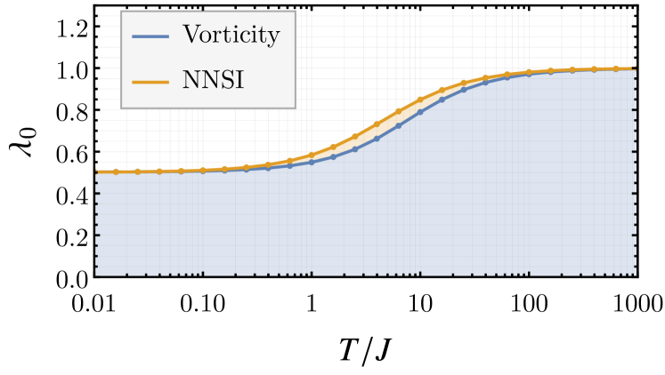
a

Figure 13: Evolution of the Lagrange multiplier $\lambda_{0}$ for both NNSI and the spin vorticity model, smoothly interpolating from 1 at high temperature to 1/2 at low temperature.

B.2 Self-Consistent Gaussian Approximation

We utilize the self-consistent Gaussian approximation (SCGA) to compute the spin-spin correlation functions, from which we obtain the spin structure factor (Eq. 10) shown in Fig. 3 of the main text. Starting from a bilinear Hamiltonian of the form of Eq. 43, we treat the $\sigma_{i}^{z}$ as real variables and add to the Hamiltonian Lagrange multipliers $\lambda_{i}T(\sigma_{i}^{z})^{2}/2$ to control the spin length, where the temperature $T$ is included for convenience. The SCGA effective Hamiltonian is then

$$H_{\text{SCGA}}=\frac{1}{2}\sum_{ij}\sigma_{i}^{z}(\lambda_{i}T\delta_{ij}+\mathcal{J}_{ij})\sigma_{j}^{z},$$ (58)

where $\delta_{ij}$ is the Kronecker delta and the $\lambda_{i}$ will be determined self-consistently by the requirement $\langle(\sigma_{i}^{z})^{2}\rangle=1$. The partition function can then be expressed as

$$Z_{\text{SCGA}}=\int\mathcal{D}\sigma_{i}^{z}\,\exp(-\frac{1}{2}\sum_{ij}\sigma_{i}^{z}(\lambda_{i}\delta_{ij}+\beta\mathcal{J}_{ij})\sigma_{j}^{z}),$$ (59)

where $\beta=1/T$. This is simply a multivariate Gaussian, and the correlation matrix can be read off,

$$\mathcal{G}_{ij}\equiv\langle\sigma_{i}^{z}\sigma_{j}^{z}\rangle=(\Lambda+\beta\mathcal{J})^{-1}_{ij},$$ (60)

with $\Lambda_{ij}\equiv\lambda_{i}\delta_{ij}$. The self-consistency conditions are then given by the requirements $\mathcal{G}_{ii}=1$. Since every site in the pyrochlore lattice is equivalent by symmetry and $\mathcal{J}$ respects the symmetries of the lattice, the solutions must be the same on every site, $\lambda_{i}\equiv\lambda$, and we only need to determine the single constant $\lambda$. Therefore, we have $\Lambda=\lambda\mathbbm{1}$ in Eq. 60, and the self-consistency condition can then be expressed as

$$\sum_{i}\langle(\sigma_{i}^{z})^{2}\rangle=\Tr\mathcal{G}=4L^{3},$$ (61)

which fixes the average total spin length squared per spin to 1. The trace is computed in the Fourier basis where $\mathcal{J}$ is $4\times 4$ block diagonal, such that

$$\Tr\mathcal{G}=\sum_{\bm{q}\in\text{FBZ}}\Tr\mathcal{G}(\bm{q}),$$ (62)

where $\mathcal{G}(\bm{q})$ is the $4\times 4$ block of $\mathcal{G}$ at wavevector $\bm{q}$ (see Eq. 40),

$$\mathcal{G}_{\mu\nu}(\bm{q})\equiv\langle\sigma_{\mu}^{z}(-\bm{q})\sigma_{\nu}^{z}(\bm{q})\rangle=(\lambda\openone_{4\times 4}+\beta\mathcal{J}(\bm{q}))_{\mu\nu}^{-1}.$$ (63)

It is furthermore convenient to shift the minimum eigenvalue of $\mathcal{J}$ to zero by defining

$$\tilde{\mathcal{J}}\equiv\mathcal{J}-\epsilon_{0}\mathbbm{1},\quad\lambda_{0}\equiv\lambda+\beta\epsilon_{0},$$ (64)

where $\epsilon_{0}$ is the minimum eigenvalue of $\mathcal{J}$. This has no influence on the physics, in particular Eq. 60 is unchanged simultaneously replacing $\lambda\to\lambda_{0}$ and $\mathcal{J}\to\tilde{\mathcal{J}}$. For NNSI, $\epsilon_{0}=-2J$, and for the spin vorticity model, $\epsilon_{0}=-6J$.

In Fig. 13, we show the evolution of $\lambda_{0}$ for NNSI and the spin vorticity model. In both cases it interpolates monotonically from $\lambda_{0}=1$ as $T\to\infty$ to $\lambda_{0}=1/2$ as $T\to 0$. At zero temperature, the correlation matrix $\mathcal{G}$ is the proportional to the projector to the flat bands. To see this, let $\bm{\psi}_{n}$ denote the $n$’th eigenvector of $\tilde{\mathcal{J}}$, with corresponding eigenvalue $\tilde{\epsilon}_{n}\geq 0$. Then, performing a spectral decomposition of $\mathcal{G}$, we obtain

$$\lim_{T\to 0}\mathcal{G}=\lim_{\beta\to\infty}\sum_{n=1}^{4L^{3}}\frac{\bm{\psi}_{n}\bm{\psi}_{n}^{\dagger}}{\lambda_{0}+\beta\tilde{\epsilon}_{n}}\to\lambda_{0}^{-1}\sum_{\mathclap{\{n|\tilde{\epsilon}_{n}=\,0\}}}\bm{\psi}_{n}\bm{\psi}_{n}^{\dagger},$$ (65)

where the final sum is over all eigenvectors with zero eigenvalue. In other words, at zero temperature $\mathcal{G}$ becomes $\lambda_{0}^{-1}$ times the projector to the null space of $\tilde{\mathcal{J}}$, which by definition is the set of its smallest eigenvalues. In NNSI and the spin vorticity model, the null space is precisely the space spanned by the eigenvectors of the flat bands, including the band touching point at $\bm{q}=\bm{0}$.

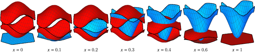
Figure 14: The bands of the interpolated interaction matrix Eq. 75, where $x=0$ gives the bands of the NNSI model and $x=1$ gives the bands of the spin vorticity model. The flat bands of NNSI (blue) become dispersive in the spin vorticity model, while the dispersive bands of NNSI (red) become flat in the spin vorticity model. This demonstrates that the two models are in a sense “reciprocal” or “complementary”, as reflected in the fact that one minimizes a divergence while the other minimizes a curl (see the discussions in Section III.1 and Section B.3). The total bandwidth at $x=0$ and $x=1$ is $8J$.

B.3 Coarse-Grained Field Theory

We can obtain a coarse-grained theory directly from the Hamiltonian, following the method of Conlon and Chalker [26], by performing a long-wavelength expansion of the interaction matrix. Expanding the vorticity interaction matrix (Eq. 51 using the parameters from Eq. 47) to quadratic order in $\bm{q}$, we obtain (denoting $|\bm{q}|^{2}\equiv q^{2}$)

$$\frac{\tilde{\mathcal{J}}^{(\text{SV})}_{\mu\nu}(\bm{q})}{J}\approx\frac{a_{0}^{2}}{2}\begin{pmatrix}q^{2}-q_{x}q_{y}-q_{y}q_{z}-q_{z}q_{x}&q_{x}q_{y}-q_{z}^{2}&q_{x}q_{z}-q_{y}^{2}&q_{y}q_{z}-q_{x}^{2}\\ q_{x}q_{y}-q_{z}^{2}&q^{2}-q_{x}q_{y}+q_{y}q_{z}+q_{z}q_{x}&-q_{y}q_{z}-q_{x}^{2}&-q_{x}q_{z}-q_{y}^{2}\\ q_{x}q_{z}-q_{y}^{2}&-q_{y}q_{z}-q_{x}^{2}&q^{2}+q_{x}q_{y}+q_{y}q_{z}-q_{z}q_{x}&-q_{x}q_{y}-q_{z}^{2}\\ q_{y}q_{z}-q_{x}^{2}&-q_{y}q_{z}-q_{x}^{2}&-q_{x}q_{z}-q_{y}^{2}&q^{2}+q_{x}q_{y}-q_{y}q_{z}+q_{z}q_{x}\end{pmatrix}.$$ (66)

We then introduce the new variables

$$Q(\bm{q}) \equiv\frac{1}{2}\sum_{\mu}\sigma_{\mu}^{z}(\bm{q}),$$ (67)

$$\bm{E}(\bm{q}) \equiv\frac{\sqrt{3}}{2}\sum_{\mu}\sigma_{\mu}^{z}(\bm{q})\hat{\bm{z}}_{\mu},$$ (68)

where $\hat{\bm{z}}_{\mu}$ are the local $[111]$ axes given by Eq. 37. Note that $Q(\bm{0})$ is the all-in-all-out (AIAO) order parameter, maximized when all $\sigma_{i}^{z}=1$, and $\bm{E}(\bm{0})$ is effectively the bulk magnetization. These variables correspond to the following unitary change of basis [26]

$$\begin{pmatrix}Q(\bm{q})\\ E^{x}(\bm{q})\\ E^{y}(\bm{q})\\ E^{z}(\bm{q})\end{pmatrix}=\frac{1}{2}\begin{pmatrix}1&1&1&1\\ 1&-1&-1&1\\ 1&-1&1&-1\\ 1&1&-1&-1\end{pmatrix}\begin{pmatrix}\sigma^{z}_{1}(\bm{q})\\ \sigma^{z}_{2}(\bm{q})\\ \sigma^{z}_{3}(\bm{q})\\ \sigma^{z}_{4}(\bm{q})\end{pmatrix}.$$ (69)

Transforming Eq. 66 to this basis, it becomes simply

$$\tilde{\mathcal{J}}^{(\text{SV})}_{\rho\sigma}(\bm{q})\approx Ja_{0}^{2}\begin{pmatrix}0&0&0&0\\ 0&q_{y}^{2}+q_{z}^{2}&-q_{x}q_{y}&-q_{x}q_{z}\\ 0&-q_{x}q_{y}&q_{x}^{2}+q_{z}^{2}&-q_{y}q_{z}\\ 0&-q_{x}q_{z}&-q_{y}q_{z}&q_{x}^{2}+q_{y}^{2}\end{pmatrix},$$ (70)

where we use $\rho,\sigma$ to denote the components in the $(Q,\bm{E})$ basis given by Eq. 69. Note that the non-zero $3\times 3$ block has matrix elements $q^{2}(\delta_{ab}-q_{a}q_{b}/q^{2})$, i.e. $q^{2}$ times the projector transverse to $\bm{q}$.

Plugging this into the SCGA effective Hamiltonian Eq. 58, accounting for Eq. 64, we obtain the effective long-wavelength (coarse-grained) theory

$$\beta H_{\text{SCGA}}^{(\text{SV})}\!\approx\!\frac{1}{2}\int\!\!\mathrm{d}^{3}\bm{q}\left[\lambda_{0}(Q^{2}+|\bm{E}|^{2})+\xi^{2}q^{2}|\hat{\bm{q}}\times\bm{E}|^{2}\right]\!,$$ (71)

with $\xi^{2}\equiv\beta Ja_{0}^{2}$. The equivalent expression for NNSI is [26]

$$\cramped{\beta H_{\text{SCGA}}^{(\text{SI})}\!\approx\!\frac{1}{2}\int\!\!\mathrm{d}^{3}\bm{q}\left[8\beta JQ^{2}+\lambda_{0}(Q^{2}+|\bm{E}|^{2})+\xi^{2}q^{2}|\hat{\bm{q}}\cdot\bm{E}|^{2}\right]\!.}$$ (72)

There are two key differences between the two coarse-grained theories. The most important is in the last term of each equation with coefficient $q^{2}$. For NNSI, the last term in Eq. 72 tells us that the single band that disperses away from the three-fold band touching point at $\bm{q}=\bm{0}$ (c.f. Fig. 3(a)) corresponds to the longitudinal component of the coarse-grained field, $\hat{\bm{q}}\cdot\bm{E}(\bm{q})$. For the spin vorticity model, the last term in Eq. 71 tells us that the two degenerate quadratically dispersing bands (c.f Fig. 3(b)) correspond to the two transverse components of the coarse-grained field, $\hat{\bm{q}}\times\bm{E}(\bm{q})$. The nature of the flat bands is revealed by separating the field into longitudinal and transverse components,

$$|\bm{E}|^{2}=|\hat{\bm{q}}\cdot\bm{E}|^{2}+|\hat{\bm{q}}\times\bm{E}|^{2},$$ (73)

and substituting back into Eqs. 71 and 72. In NNSI the two transverse components lack dispersion and thus correspond to the two flat bands, while in the spin vorticity model both the longitudinal component of $\bm{E}$ as well as the scalar $Q$ lack dispersion, thus constituting the two flat bands.

The second difference is the role of $Q$, which in NNSI corresponds to the upper band that is gapped at zone center with maximum energy $8J$. Since it is gapped in NNSI, it can be integrated out entirely and ignored in the coarse-grained theory describing the low-energy description [26]. In the spin vorticity model, by contrast, the AIAO state maximizing $Q(\bm{0})$ is a ground state, along with the three fully-polarized configurations maximizing $\bm{E}(\bm{0})$, corresponding to the fourfold degeneracy at $\bm{q}=\bm{0}$ in the bands of the spin vorticity model interaction matrix (see Fig. 3(b)).

B.4 Interpolation to NNSI

To visualize the “reciprocal” relationship between the spin vorticity model to the nearest-neighbor spin ice (NNSI) model, we can look at how their bands evolve as we interpolate between them. The NNSI interaction matrix is proportional to the nearest-neighbor adjacency matrix of the pyrochlore lattice,

$$\mathcal{J}_{ij}^{(\text{NNSI})}=J\mathcal{A}_{ij}^{(1)}.$$ (74)

We define a continuum of models interpolating from NNSI to the spin vorticity model defined by the interaction matrices

$$\tilde{\mathcal{J}}^{\text{interp}}(x)=(1-x)\tilde{\mathcal{J}}^{(\text{NNSI})}+x\,\tilde{\mathcal{J}}^{(\text{SV})},$$ (75)

where for convenience we keep the minimum eigenvalue at zero according to Eq. 64. In Fig. 14, we show the evolution of the bands as $x$ varies from $0$ (NNSI) to 1 (vorticity model). The blue bands are flat and degenerate in the NNSI model, corresponding to the extensively degenerate ground state of closed head-to-tail configurations with zero divergence (the rotational component of the Helmholtz decomposition). Conversely, the red bands are flat and degenerate in the spin vorticity model, corresponding to the irrotational (curl-free) component of the Helmholtz decomposition and the degenerate ground states of the spin vorticity model made of closed membranes. One may directly verify that $\tilde{\mathcal{J}}^{(\text{NNSI})}$ and $\tilde{\mathcal{J}}^{(\text{SV})}$ commute, and thus share a common eigenbasis. Therefore, only the eigenvalues of $\tilde{\mathcal{J}}^{\text{interp}}(x)$ vary as a function of $x$, and not the eigenvectors, meaning that the character of the bands as either irrotational (red) or rotational (blue) does not change as the bands deform.

Appendix C Monte Carlo Simulations

This Appendix provides details of the Monte Carlo simulations and data analysis described in the main text Section III.2.

C.1 Sampling and Star Moves

We compute spin-spin correlation functions and other thermodynamic observables by averaging over $N_{\text{samp}}$ sample configurations at each temperature, generated by Markov chain Monte Carlo simulations performed for an $L\times L\times L$ FCC lattice with periodic boundaries, containing $4L^{3}$ spins. Simulations for NNSI are performed using the extremely efficient algorithm introduced by Otsuka [71], see therein for details. This algorithm splits the entire spin configuration into closed and open strings, which are flipped with 50/50 probability. Since the autocorrelation times are extremely short, we take a sample after each iteration of the algorithm.

For the spin vorticity model, we utilize both single spin flips and “star moves” (Section III.2) to thermalize the system. A star move flips an all-out tetrahedron to an all-in tetrahedron or vice-versa—for the spin vorticity Hamiltonian, this cluster move costs zero energy. For single spin flips, we choose a random spin to flip, accepting or rejecting according to the Metropolis condition, i.e. with probability $\text{min}[1,\exp(-\beta\Delta E)]$, where $\beta$ is inverse temperature and $\Delta E$ is the change in the total energy due to the flip. For star moves, we pick a random tetrahedron and flip it if it is all-in or all-out—this move satisfies detailed balance since the before and after configurations have the same energy and the transition probability in either direction is the same. We take a sample configuration after each sweep of the lattice, where a single sweep means applying $4L^{3}$ single spin flip attempts and $2L^{3}$ star move attempts. At temperatures well below the minimum excitation energy scale of $6J$, where the vorticity spin liquid phase is well-formed, single spin flips are exponentially suppressed.

C.2 Partial AIAO Order

The pattern of Bragg peak intensities in the structure factor $S(\bm{q})$ (Eq. 10) seen in Fig. 4(d) is indicative of all-in-all-out (AIAO) ordering. To see this, first note that for a fully-ordered AIAO configuration, i.e. one with every $\sigma_{i}^{z}=1$, we can directly compute $S(\bm{q})$. Splitting the sum over pyrochlore sites $i$ into a sum over FCC and sublattice positions (Eq. 35), the double sum over FCC vectors yields a Kronecker delta restricting $\bm{q}$ to be a reciprocal lattice vector,

$$S_{\text{AIAO}}(\bm{q})=\left(L^{3}\sum_{\mu,\nu}e^{i\bm{q}\cdot(\bm{c}_{\nu}-\bm{c}_{\mu})}\right)\delta_{\bm{q},\sum_{k}m_{k}\bm{b}_{k}}\quad(m_{k}\in\mathbbm{Z}).$$ (76)

The intensity at each zone center can differ due to interference of the sublattice phase factors, yielding three symmetry-distinct zone centers Bragg peak intensities. Inserting Eq. 34, we find

$$S_{\text{AIAO}}(\bm{q})=\begin{cases}16L^{3}&\quad\bm{q}=(000),\\ 4L^{3}&\quad\bm{q}=(111),\\ 0&\quad\bm{q}=(002).\end{cases}$$ (77)

As observed in the main text Fig. 4(d) as well as in Fig. 15, the zero-temperature Bragg peak intensities measured in Monte Carlo for the spin vorticity model satisfy precisely the ratios (4:1:0) expected for AIAO order, but with the peak intensities only about $0.4\%$ of those given in Eq. 77.

\begin{overpic}[width=398.9296pt]{Figures/linecuts.pdf} \put(-4.0,80.0){(a)} \put(-4.0,53.0){(b)} \put(-4.0,26.0){(c)} \put(-4.0,-3.0){(d)} \put(51.0,-3.0){(e)} \end{overpic}

\begin{overpic}[width=182.1196pt]{Figures/lc_reference.pdf} \put(-2.0,1.5){$\bar{4}$} \put(-2.0,18.2){$\bar{2}$} \put(-2.0,35.5){0} \put(-2.0,53.0){2} \put(-2.0,70.0){4} \put(1.5,-3.0){$\bar{4}$} \put(25.5,-3.0){$\bar{2}$} \put(50.5,-3.0){0} \put(74.5,-3.0){2} \put(98.5,-3.0){4} \end{overpic}

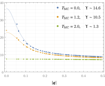
Figure 15: (a,b,c): Line cuts of the spin structure factor $S(\bm{q})$ for the spin vorticity model at three temperatures. Filled dots show Monte Carlo data for temperatures $T_{\text{MC}}=2.0,1.2,0.0$, averaged over $10^{5}$ samples at each temperature with $L=32$. The Bragg peaks are noted with arrows indicating their intensities. As noted in the main text, $S(\bm{0})$ is only about $0.4\%$ of the expected value for complete AIAO order of $16L^{3}=524\,288$ for this system size. Thick transparent lines show the SCGA result for temperatures $T_{\text{SCGA}}=2.0,0.63,0.001$, chosen to quantitatively match the diffuse intensity. Note that in the SCGA, $S(\bm{q})$ is constant along the highest-symmetry lines $(00h)$ and $(hhh)$. (d) $S(\bm{q})$ in the $(hhl)$ plane from which the line cuts above were taken, with the five cut lines indicated. (e) Lorentzian fits of the tails surrounding the $\bm{q}=\bm{0}$ Bragg peak, in the region $|\bm{q}|\lesssim 0.5$, at the same three temperatures as (a,b,c)

C.3 Line Cuts of Structure Factors

In Fig. 15, we provide line cuts of the Monte Carlo measurement of the spin structure factor $S(\bm{q})$ (Eq. 10) appearing in Fig. 4(b,c,d) in the main text. Monte Carlo data points are shown by colored points, connected by thin solid lines as a guide to the eye. For comparison, we also show the same line cuts computed in the SCGA, shown as thick transparent lines. Note that because of the "softening" of the spin length constraint in the SCGA, observables computed at a fixed temperature $T$ in both SCGA and Monte Carlo will not necessarily agree, since the “hard” Ising spin length constraint in Monte Carlo means there is a finite energy gap to excitations, while in the SCGA the soft spins can fluctuate continuously. Thus we compare Monte Carlo data at temperature $T_{\text{MC}}$ with SCGA data at a temperature $T_{\text{SCGA}}$, the latter of which is chosen to give a good quantitative fit of the structure factor in the diffuse regions away from zone centers.

The primary feature differentiating the Monte Carlo results from the SCGA is the presence of the sharp Bragg peaks surrounded by Lorentzian-like “tails”. These tails begin to form above $T_{*}$, and maintain a finite width all the way to zero temperature, despite the formation of delta-function Bragg peaks. We emphasize that the SCGA tracks the development of the diffuse correlations of the spin liquid, away from the Bragg peaks, to a high degree of precision at all temperatures, i.e. we can always find an SCGA temperature $T_{\text{SCGA}}$ at which the SCGA quantitatively agrees with the Monte Carlo data in the diffuse region. The second difference between the SCGA and Monte Carlo data is the loss of pinch point intensity at the (002) position in the Monte Carlo data at the lowest temperature. This loss of intensity is visible in the $(hh2)$ cut (yellow) at $h=0$, in the $(hh0)$ cut (red) at $h=\pm 2$, and in the $(00h)$ cut (green) at $h=\pm 2$. We argued in Section IV.4.1 that this loss is due to the lack of topological sector fluctuations at low temperatures, since we do not have at hand an explicit cluster move that changes the topological sector.

In the bottom right panel of Fig. 15 we also show the shape of the tails surrounding the zone-center Bragg peak as a function of $|\bm{q}|$ in units of $2\pi/a_{0}$ in the long-wavelength region $|\bm{q}|\lesssim 0.5$. The tails can be fit to Lorentzians of the form

$$f(\bm{q})=C+\frac{A}{1+\Upsilon^{2}|\bm{q}|^{2}},$$ (78)

where $C$ accounts for the near-constant background intensity which is predicted by the SCGA. The quantity $\Upsilon$ may be interpreted as a correlation length, which saturates to a value on the order of $\Upsilon\sim 10^{1}$ at low temperature. This lengthscale does not diverge at the transition, increasing monotonically from zero at high temperature to a finite value at $T=0$, without diverging at the transition temperature $T_{*}$.

C.4 Specific Heat and Entropy

For the specific heat data shown in the main text Fig. 4(a), $N_{\text{samp}}=10^{5}$ samples were averaged at each temperature for a system with $L=32$. The specific heat is measured as the variance of the energy divided by temperature squared,

$$c(T)=\frac{1}{4L^{3}}\frac{\langle E^{2}\rangle-\langle E\rangle^{2}}{T^{2}}.$$ (79)

Uncertainties in the statistical averages are estimated via Jackknife resampling.

The entropy per spin, $s(T)$, is computed by integrating $c/T$ as

$$s(T)=s(\infty)+\int_{\infty}^{100J}\mathrm{d}T^{\prime}\frac{c(T^{\prime})}{T^{\prime}}+\int_{100J}^{T}\mathrm{d}T^{\prime}\frac{c(T^{\prime})}{T^{\prime}},$$ (80)

where $s(\infty)=\ln(2)$. The first integral in Eq. 80 contains the entropy released between $T/J=\infty$ and $T/J=100$, the highest temperature measured, which is estimated as follows. Over this range, the specific heat is approximated by its higher-temperature series form,

$$c(T)\approx aT^{-2}+bT^{-3},$$ (81)

where the leading term goes as $T^{-2}$ since the variance of the energy in Eq. 79 is constant at high temperature. We therefore fit $c(T)T^{2}$ versus $T^{-1}$ between $T/J=50$ and $T/J=100$ to a linear function $a+bx$ (where $x=T^{-1}$) to extract the values of $a$ and $b$, from which we obtain

$$\int_{\infty}^{100J}\mathrm{d}T^{\prime}\frac{c(T^{\prime})}{T^{\prime}}\approx-\frac{150a+b}{3\times 10^{6}}$$ (82)

$$\qquad=\begin{cases}-(2.59\pm.02)\times 10^{-4}&\quad\text{vorticity},\\ -(1.47\pm.02)\times 10^{-4}&\quad\text{NNSI}.\end{cases}$$ (83)

The remaining entropy release below $T/J=100$ (the second integral in Eq. 80) is computed by interpolating the $c(T)$ data and integrating numerically.

The uncertainties in the integrated quantities are computed by resampling the data: each data point whose average and standard deviation is measured in Monte Carlo is treated as a random Gaussian variable to generate $N_{\text{resamp}}$ new $c(T)$ data sets, for each of which $s(T)$ is computed by numerical integration. The resulting values are averaged and their standard deviation is taken as the uncertainty, indicated by the error bars in Fig. 4(b) in the main text. We find that the averages and uncertainties have converged well for $N_{\text{resamp}}\sim 10^{2}$, and the reported values are given for $N_{\text{resamp}}=10^{3}$.

C.5 Pinch Points and Topological Sector Fluctuations

As noted in the main text, the intensity of the structure factor $S(\bm{q})$ for the spin vorticity model at the $\bm{q}=(002)$ pinch point location is zero at low temperatures in our Monte Carlo simulations. In Section IV.4.1 we argued that this is because our star move algorithm is not fully ergodic, since it is not capable of changing the topological sector of a configuration. The topological sectors are indexed by $\bm{E}(\bm{q}=\bm{0})$ (Eq. 68), which is proportional to the bulk magnetization. To see this, first define the net moment of a single tetrahedron,

$$\bm{E}_{t}\equiv\frac{\sqrt{3}}{2}\sum_{i\in t}\sigma_{i}^{z}\hat{\bm{z}}_{i},$$ (84)

in terms of which the bulk moment is

$$\bm{E}(\bm{0})=\frac{1}{2}\sum_{t}\bm{E}_{t},$$ (85)

where the factor of 1/2 accounts for double counting. Consider first a zero-magnetization all-in-all-out configuration, e.g. every $\sigma_{i}^{z}=+1$, which is a ground state of the spin vorticity model and has $\bm{E}_{t}=\bm{0}$ on every tetrahedron. The minimal membrane move is the star move, flipping an all-out tetrahedron to an all-in tetrahedron or vice versa, and this clearly does not affect $\bm{E}(\bm{0})$ since $\bm{E}_{t}=\bm{0}$ for this tetrahedron before and after. Next, note that any non-winding closed membrane flip is equivalent to a sequence of star moves on every tetrahedron inside the membrane, so these also cannot change $\bm{E}(\bm{0})$. Now consider a membrane which winds around the periodic boundaries, for example a flat plane orthogonal to $[111]$ cutting one of the triangular sublattices of the pyrochlore lattice (Fig. 7(b) in the main text shows a portion of such a flat membrane). For each tetrahedron on either side of this membrane, the moment becomes $\bm{E}_{t}=\sqrt{3}\hat{\bm{z}}_{1}/2$, so the net moment becomes $\bm{E}(\bm{0})=N_{\Delta}\sqrt{3}\hat{\bm{z}}_{1}$, where $N_{\Delta}$ is the number of plaquettes in the membrane (i.e. the number of flipped spins). We conclude that the value of $\bm{E}(\bm{0})$ depends only on the topological sector

The intensity of the pinch point at $(002)$, where there is no AIAO Bragg peak, is proportional to $\langle|E^{z}(\bm{0})|^{2}\rangle$. To see this, first note that the spin structure factor, Eq. 10 in the main text, can be expressed as

$$S(\bm{q})=4\langle|Q(\bm{q})|^{2}\rangle,$$ (86)

with $Q(\bm{q})$ defined in Eq. 67. Now note that from Eq. 38,

$$\sigma_{\mu}(\bm{q}+\bm{k})=\sigma_{\mu}^{z}(\bm{q})e^{-i\bm{k}\cdot\bm{c}_{\mu}},$$ (87)

so that we can expand Eq. 67,

$$Q((002)+\bm{k}) =\frac{1}{2}\sum_{\mu}\sigma_{\mu}^{z}(\bm{k})e^{-i(002)\cdot\bm{c}_{\mu}}$$ (88)

$$=\frac{1}{2}\sum_{\mu}\sigma_{\mu}^{z}(\bm{k})(-\sqrt{3}\hat{\bm{z}}\cdot\hat{\bm{z}}_{\mu})$$ (89)

$$=-\hat{\bm{z}}\cdot\bm{E}(\bm{k}),$$ (90)

where $\hat{\bm{z}}$ is the global Cartesian $z$-axis unit vector along [001]. We thus conclude that

$$S((002)+\bm{k})=4\langle|E^{z}(\bm{k})|^{2}\rangle,$$ (91)

and, in particular,

$$S((002))=4\langle|E^{z}(\bm{0})|^{2}\rangle.$$ (92)

Thus the pinch point intensity of $S(\bm{q})$ at the $(002)$ zone center is proportional to the fluctuation of $E^{z}(\bm{0})$, which measures the fluctuation between topological sectors. Its extinction in Fig. 4(d) in the main text is indicative of the lack of topological sector updates at low temperature using only local single spin flip and star move updates.

\begin{overpic}[width=368.57964pt]{Figures/gauss_law_flux.pdf} \put(50.0,0.0){(a)} \put(50.0,-100.0){(b)} \end{overpic}

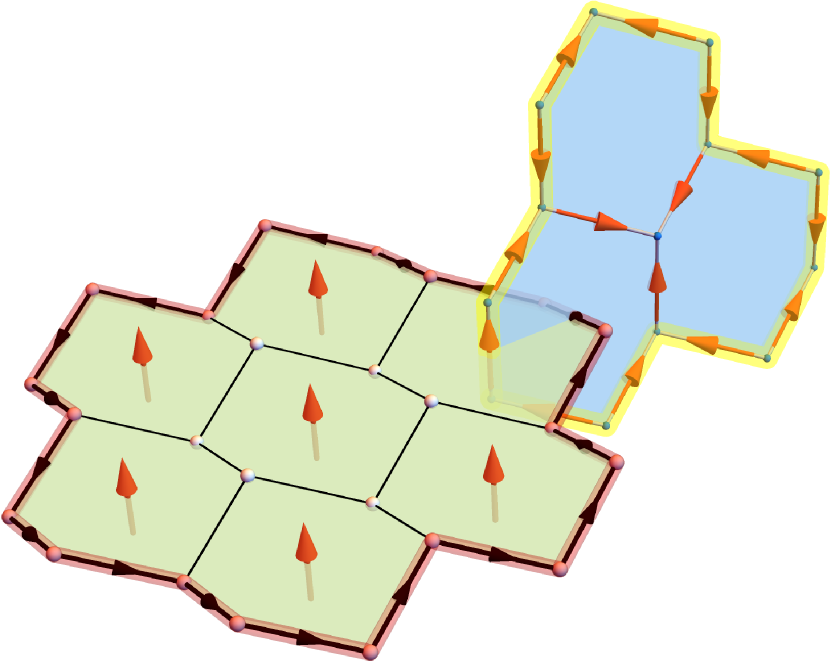
Figure 16: (a) In spin ice, the charge excitations are detected by integrating the amount of flux through a closed surface in the dual lattice. The string (yellow) attached to the charge is not uniquely defined, but the intersection number of the string in the direct lattice and the closed surface in the dual lattice counts the amount of charge enclosed, independent of the string position. (b) In the spin vorticity model, the excitations are charged strings (red), and these are detected by integrating the circulation of the spins around a loop in the direct lattice (yellow). This loop links the string excitations and pierces the flux membranes (green). The signed intersection of the loop with the membrane counts the number of string excitations linked by the loop.

Appendix D Topological Strings and Membranes on the Lattice

The strings of spin ice and the membranes of the spin vorticity model play complementary roles in the two models. In spin ice, the constraint $Q_{t}=0$ enforces that the electric strings cannot have open ends, while its violation is sourced by a charge at each open end of a string. In Maxwell theory, the presence of the charge is detected by integrating the Gauss law $\nabla\cdot\bm{E}=\rho$ (with $\rho$ the charge density) over a volume $V$, which by Gauss’s theorem is equivalent to

$$\iiint_{V}(\nabla\cdot\bm{E})\,\mathrm{d}V\equiv\oiint_{\partial V}\bm{E}\cdot\mathrm{d}\bm{S}=Q_{\text{enc}},$$ (93)

where $Q_{\text{enc}}$ is the charge enclosed by the surface $\partial V$ which bounds $V$, and the surface is oriented “out”. Thus a positive charge within the volume corresponds to a net flux of electric field lines out through its surface.

In the lattice, these surfaces necessarily should live in the dual lattice, such that they surround the vertices of the direct lattice and are pierced by the links of the direct lattice. This is depicted in Fig. 16(a), which shows a closed surface in the dual lattice (green) surrounding a point charge (black) at the end of an electric string (yellow) in the direct lattice. Using the notation introduced in Eq. 19, we can write the lattice equivalent of Eq. 93,

$$\sum_{\tilde{p}\in\partial{\tilde{V}}}S^{z}_{\tilde{p}}=\sum_{t\in\tilde{V}}Q_{t},$$ (94)

where $\tilde{V}$ is a volume in the dual lattice. Note that the position of the electric string is not uniquely defined, but the signed intersection number of the electric string and the closed surface counts the number of charges inside the surface, where the signed intersection of a $k$-dimensional objects and a $(d-k)$-dimensional object ($d$ being the dimension of space) is $+1$ if they intersect with the same orientation and $-1$ if they intersection with opposite orientation.

In the spin vorticity model, the constraint $\omega_{p}=0$ enforces that the spins arrange into closed electric membranes. Violations of this constraint appear as closed charged strings in the dual lattice, which are detected by computing the circulation of the spins around a closed loop which links the string. In Maxwell theory, these strings may be considered analogous to a loop of current, coupled to the field by an Ampere’s law,

$$\nabla\times\bm{E}=\bm{\mathscr{j}},$$ (95)

which reads in integral form

$$\oint_{\partial U}\bm{E}\cdot\mathrm{d}\bm{\ell}=\iint_{U}\bm{\mathscr{j}}\cdot\mathrm{d}\bm{S},$$ (96)

where $U$ is any surface. This equation tells us that the circulation of the field around any closed loop counts the amount of current flowing through a surface $U$ which has that loop as its boundary. To write the lattice version of the Ampere law Eq. 96, we utilize Eq. 16 and sum the vorticity over all plaquettes forming a surface $\Sigma$ in the direct lattice to obtain

$$\sum_{\ell\in\partial\Sigma}S_{\ell}^{z}=\sum_{p\in\Sigma}\omega_{p},$$ (97)

and identify $\omega_{p}=\mathscr{j}_{\tilde{\ell}}$. This equation then states that the circulation of the spins around $\partial\Sigma$ is equal to the number of strings piercing the surface $\Sigma$, i.e. linking $\partial\Sigma$. This is depicted in Fig. 16(b), which shows a single string (red) in the dual lattice attached to a membrane (green). It is linked by a closed contour (yellow) in the direct lattice, on the boundary of a surface $\Sigma$ (blue). The circulation of $S^{z}$ around the yellow contour counts the number of strings piercing the blue surface $\Sigma$, which is the signed intersection number of the surface with the string.

Utilizing these microscopic definitions, we can define topological winding numbers for both spin ice and the vorticity model ground states. In spin ice, where ground state configurations have zero divergence, the topological sector is determined by the number of electric strings piercing a topologically non-trivial surface $\Sigma$ in the dual lattice,

$$w[\Sigma]:=\sum_{\tilde{p}\in\Sigma}S^{z}_{\tilde{p}},$$ (98)

which depends only on the homology class of $\Sigma$ [77], i.e. which of the three holes of the torus $\Sigma$ winds around, and is invariant under the flipping of a contractible loop of head-to-tail spins. The number $w[\Sigma]$ is zero if $\Sigma$ is contractible, since it is equivalent by Eq. 94 to the total divergence inside the volume bounded by $\Sigma$. In the vorticity model, the topological sector of a ground state is defined by the winding number around non-contractible loops $C$ in the direct lattice,

$$w[C]:=\sum_{\ell\in C}S_{\ell}^{z},$$ (99)

which depends only on the homology class of $C$, i.e. which hole it winds around, and is invariant under the flipping of contractible membranes. The number $w[C]$ is zero if $C$ is contractible, since by Eq. 97 it is equal to the total vorticity on a set of plaquettes forming a surface bounded by $C$.

\begin{overpic}[width=281.85034pt]{Figures/hard_hexagons.pdf} \put(-15.0,80.0){(a)} \put(-15.0,-25.0){(b)} \end{overpic}

\begin{overpic}[width=281.85034pt]{Figures/incommensurability.pdf} \put(16.0,65.0){$\omega_{p}=+2$} \put(43.0,27.0){$\omega_{p}=-3$} \put(63.0,65.0){$\omega_{p}=+3$} \end{overpic}

Figure 17: (a) Spin configurations can be mapped to hard-plaquette coverings of the dual diamond lattice by identifying the two Ising states (indicated with red arrows) relative to a reference orientation (black arrowheads) with the presence or absence of a hard hexagon (dark gray). (b) In order to turn the ground state constraint $\omega_{p}=0$ into a local constraint on edge-touching of hard hexagons, one should choose a reference orientation where every hexagon is fully polarized with $|\omega_{p}|=3$. However, there is no such spin orientation due to the way that the direct-lattice hexagons touch at their corners. Here we show a configuration with two fully-polarized hexagons, which forbids the third hexagon from being fully polarized.

\begin{overpic}[width=433.62pt]{Figures/kagome_vorticity_duality.pdf} \put(22.0,-2.0){(a)} \put(75.8,-2.0){(b)} \end{overpic}

Figure 18: (a) A portion of the kagomé lattice with Ising spins represented by red arrows oriented along the parent honeycomb lattice edges. Comparing to Fig. 1(a), the kagomé lattice plays the role of the pyrochlore lattice while the honeycomb lattice plays the role of the diamond lattice. Defining a kagomé version of the vorticity model whose Hamiltonian is given by Eq. 8 with vorticity defined on each hexagonal plaquette (one highlighted blue) according to Eq. 7 (relative to an AIAO basis), ground states have zero circulation around each plaquette. The spin configuration shown here satisfies the ground state constraint on the five shown hexagons. The dual lattice of the honeycomb is a triangular lattice, shown transparent in the background. The analog of a closed membrane in two dimensions in a closed curve. The green string highlighted on the dual triangular lattice intersects five spins, all of which point “out”, analogous to the closed membranes in Fig. 6(b,c). Flipping these spins does not change the circulation around any plaquette and thus does not change the energy, analogous to the membrane flips in the 3D spin vorticity model. Thus in a 2D spin vorticity model, the analog of the two-dimensional membranes are one-dimensional strings. (b) This model can be mapped to an ice model on the dual triangular lattice by simply rotating each spin vector by ninety degrees in the plane so that they point along the edges of the triangular lattice. The zero-vorticity constraint then becomes a zero divergence constraint in the dual model, i.e. a 3-in-3-out ice rule, which can be visually seen to be satisfied at the five vertices in the interior, each with six surrounding spins. The green string in the vorticity model in (a) becomes a string of head-to-tail spins in the ice model in (b), and flipping this string does not change the divergence at any triangular lattice vertex. This is because curl and divergence are dual operations in two dimensions. Thus two-dimensional spin vorticity models are dual to two-dimensional spin ice models.

Appendix E Dimers versus Hard-Plaquette Coverings

It is worth considering how to think of the spin vorticity model in terms of dimer models, which play an important role in the understanding of liquid phases based on resonating valence bonds as well as in spin ice [83]. This is done by mapping the two spin states with respect to a chosen reference configuration to the presence or absence of a dimer. In NNSI, we take the reference configuration to be an AIAO state, with the dimers covering the bonds of the diamond lattice. Then the two-in/two-out constraint $Q_{t}=0$ translates to the constraint that exactly two dimers touch at each vertex (diamond site), such that the ground states of NNSI are in one-to-one correspondence with closed-string coverings of the diamond lattice with dimers [21, 83]. It turns out that no such mapping exists for the spin vorticity model, which we now demonstrate.

The dimer language to express the constraint $\omega_{p}=0$ in the spin vorticity model is more complicated than its usage in the NNSI case. Let us take the AIAO configuration as our reference state, so that $\sigma_{i}^{z}=+1$ ($-1)$ corresponds to the presence (absence) of a dimer on each edge. Separating the six edges direct diamond edges around the hexagonal plaquette in Fig. 2 into the even and odd subsets, the constraint $\omega_{p}=0$ translates to covering an equal number of even and odd edges by a dimer. Expressed in this way, the constraint appears non-local and ad-hoc, and one may wonder whether there is a more natural description. In spin ice, the dimer-touching constraint corresponds to the local zero-charge constraint $Q_{t}=0$ at each diamond vertex, so it is natural to search for a similar touching constraint equivalent to $\omega_{p}=0$, but located on the dual diamond lattice edges, where the string excitations live. Thus we consider mapping the Ising states $\sigma_{i}^{z}=\pm 1$ to the presence or absence of a hard plaquette on the corresponding dual plaquette, rather than a dimer on the corresponding direct edge. This is illustrated in Fig. 17(a), with six spins forming a $|\omega_{p}|=3$ configuration which map, relative to all-in-all-out configuration (indicated by small black arrowheads), to the presence of three hard hexagons (dark gray).

Switching from dimers to hard hexagons does not solve the issue of the ad-hoc constraint by itself, instead we need to choose a different basis in which the constraint $\omega_{p}=0$ translates to the constraint that three hard hexagons touch at each dual edge. For a single plaquette $p$, this is achieved precisely when we choose the reference configuration to be one of the two maximally-circulating $\omega_{p}=\pm 3$ configurations, relative to which an $\omega_{p}=0$ configuration corresponds to choosing any three of the six $\sigma_{i}^{z}$ on the hexagon to be $-1$. Then the constraint says that exactly three hard hexagons touch at the dual lattice edge passing through plaquette $p$. This is exactly analogous to spin ice, where the reference configuration is one of the two all-in all-out configurations and the constraint $Q_{t}=0$ says that any two of the $\sigma_{i}^{z}$ on a tetrahedron are chosen to be $-1$. However, unlike the all-in-all-out configuration for which every tetrahedron satisfies $|Q_{t}|=2$, there is no spin configuration for which every plaquette satisfies $|\omega_{p}|=3$. This is illustrated in Fig. 17(b), which shows that two adjacent hexagons can be chosen to have opposite maximal circulation, but a third hexagon sharing a spin with both of them cannot be assigned a maximal circulation configuration. Thus there is no hard-hexagon mapping where the constraint $\omega_{p}=0$ becomes a simple local constraint that three hard-hexagons touch at each dual lattice edge, such that the system is at half filling in the ground state.

Appendix F 2D Vorticity Models: Duality with Ice Models

One may wonder why the spin vorticity model we defined in Eq. 8 and discussed throughout this section should be defined in three spatial dimensions. One can indeed define a spin vorticity model on a 2D lattice such as the kagomé. It is straightforward to see that the resulting model is in fact dual to an ice model, due to a duality in two dimensions of curl and divergence, and thus does not result in 2-form spin liquidity.

To see this, consider an Ising model on the kagomé lattice, shown in LABEL:fig:kagom\'e_vorticity_duality(a) with arrows (red) indicating the directions of the local spins. For each plaquette $p$ of the parent honeycomb lattice, one of which is colored blue, we can define the vorticity $\omega_{p}$ identical to Eq. 7, and a spin vorticity model with Hamiltonian given by Eq. 8 which includes first, second, and third neighbor interactions whose ground states minimize the circulation around every plaquette. The dual lattice of the parent honeycomb lattice is a triangular lattice, shown transparent in the background. A “membrane” in the dual triangular lattice is traced (green) which intersects five spins, all of which point “out”, but clearly in two spatial dimensions this is in fact a 1-dimensional string, not a 2-dimensional surface. Flipping this “membrane” generates another configuration with the same energy since it does not change the circulation around any plaquette.

Indeed, these strings are in fact the strings of a spin ice model defined on the dual lattice. Each spin configuration in LABEL:fig:kagom\'e_vorticity_duality(a) may be mapped to a configuration of spins sitting on the links of a triangular lattice, by simply rotating every red arrow by ninety degrees in the plane, shown in LABEL:fig:kagom\'e_vorticity_duality(b). Each direct plaquette with zero vorticity becomes a vertex with zero divergence in the dual system. This can be seen in LABEL:fig:kagom\'e_vorticity_duality, where the blue plaquette has zero circulation in (a), and the corresponding vertex satisfies a 3-in-3-out ice rule in (b). This is a natural consequence of the fact that in two dimensions, the curl and divergence operators are dual [3]. Given a vector field $\bm{E}=E_{x}\hat{\bm{x}}+E_{y}\hat{\bm{y}}$, define its dual field $\bm{E}^{\prime}=-E_{y}\hat{\bm{x}}+E_{x}\hat{\bm{y}}$, then $\nabla\cdot\bm{E}=\nabla\times\bm{E}^{\prime}$ and $\nabla\times\bm{E}=-\nabla\cdot\bm{E}^{\prime}$, where the two-dimensional curl is a scalar defined by $\nabla\times\bm{E}=\partial_{x}E_{y}-\partial_{y}E_{x}$. This curl-divergence duality was utilized in Ref. [156] to study 2D ice models, and is also utilized to define height model representations of 2D lattice Coulomb phases [79, 3]. We conclude that in two dimensions, there is a natural duality between spin vorticity models, which enforce a zero-curl constraint, and ice models, which enforce a zero-divergence constraint—both result in traditional Coulomb phases [3]. In the spin ice model the excitations are charges, while in the spin vorticity model they are vortices, so this may be viewed as a simple manifestation of the phenomenon of particle-vortex duality [126].

Appendix G p-Form Gauge Theory

In this Appendix, we summarize for the interested reader some basic concepts of higher-form gauge theory in comparison to the more familiar 1-form gauge theory. We first provide a very brief elementary description of differential forms and exterior calculus. The primary mathematical idea the reader should be aware of is that (i) a $p$-form is a rank-$p$ antisymmetric tensor field, and (ii) a $p$-form can be integrated in a well-defined way over a $p$-dimensional surface. The overarching physical principle of $p$-form gauge theory is that a U(1) $p$-form gauge potential $A$ encodes the parallel transport of a charged $(p-1)$-dimensional object, which sweeps out a $p$-dimensional worldline through spacetime [47].

In the familiar case $p=1$, a 1-form gauge potential encodes the total phase accumulated by a charged point particle traversing through the gauge field along its worldline $c$, given by $\exp(i\int_{c}A)$. In the case $p=2$, a 2-form gauge potential encodes the phase accumulated by a string moving through a generalized electromagnetic field, $\exp(i\iint A)$, where the surface integral is taken over the worldsheet of the string [47]. Because there is no notion of a path ordering for surfaces or higher-dimensional “branes”, $p$-form gauge fields with $p>1$ must have Abelian gauge groups [47], unless one replaces the gauge group with a generalized object called a higher group [157].

G.1 Differential Forms and Exterior Calculus

We start with a brief overview of differential forms, a more detailed account can be found in differential geometry textbooks, for example, see Chapters 5 and 7 of Nakahara [158]. A 0-form is simply a scalar function, while a 1-form may be equated to a vector field. In three-dimensional space, a 2-form may be equated to a pseudovector field and a 3-form to a pseudoscalar function (pseudo indicating that these change sign under spatial inversions). In Maxwell electrodynamics, the electric vector field $\bm{E}$ is naturally integrated along a 1-dimensional contour, and is properly viewed as a 1-form, $\cramped{E\equiv\bm{E}\cdot\mathrm{d}\bm{\ell}}$; the magnetic vector field $\bm{B}$ is naturally integrated over a 2-dimensional surface, and is properly viewed as a 2-form, $\cramped{B\equiv\bm{B}\cdot\mathrm{d}\bm{S}}$; and the charge density $\rho$ is naturally integrated over a volume, and is properly viewed as a 3-form, $\cramped{\rho\,\mathrm{d}V}$.

Consider a set of $d$ basis 1-forms, denoted $\mathrm{d}x^{\mu}$, $\mu=1,\ldots d$ where $d$ is the dimension of space. One may think of this as a set of $d$ linearly independent vector fields. We can expand a 1-form, a 2-form, and a 3-form in this basis in terms of their components as

$$\alpha =\phantom{\frac{1}{2!}}\,\alpha_{\mu}\,\mathrm{d}x^{\mu},$$

$$\beta =\frac{1}{2!}\,\beta_{\mu\nu}\,\cramped{\mathrm{d}x^{\mu}\wedge\mathrm{d}x^{\nu}},$$

$$\gamma =\frac{1}{3!}\,\gamma_{\mu\nu\rho}\,\cramped{\mathrm{d}x^{\mu}\wedge\mathrm{d}x^{\nu}\wedge\mathrm{d}x^{\rho}},$$ (100)

with implied summation over repeated indices. The components of a $p$-form, e.g. $\gamma_{\mu\nu\rho}$ for $p=3$, are a collection of $p!$ functions of position, completely antisymmetric with respect to exchanging indices. A 0-form is just a single function. The wedge product $\wedge$ is the anti-symmetrized tensor product, meaning that

$$\cramped{\mathrm{d}x^{\mu}\wedge\mathrm{d}x^{\nu}}=-\cramped{\mathrm{d}x^{\nu}\wedge\mathrm{d}x^{\mu}}.$$ (101)

The basis elements $\cramped{\mathrm{d}x^{1}\wedge\cdots\wedge\mathrm{d}x^{p}}$ play the role of the $p$-dimensional infinitesimal integration measures, such as $\mathrm{d}\bm{\ell}$, $\mathrm{d}\bm{S}$, and $\mathrm{d}V$. The complete antisymmetry of these basis elements encodes a reversal of sign under a reversal of orientation. The factorial prefactors remove over-counting of the contracted components and basis elements, since for example $\cramped{\beta_{12}\mathrm{d}x^{1}\wedge\mathrm{d}x^{2}=\beta_{21}\mathrm{d}x^{2}\wedge\mathrm{d}x^{1}}$.

We now introduce the exterior derivative, which may be viewed as a generalized notion of gradient for $p$-forms. The exterior derivative $\mathrm{d}_{p}$ sends a $p$-form $\omega$ to a $(p+1)$-form, denoted $\mathrm{d}_{p}\omega$, whose components are given by gradients of the components of $\omega$,

$$\mathrm{d}_{p}\omega=\frac{1}{p!}\partial_{\mu_{1}}\omega_{\mu_{2}\cdots\mu_{p+1}}\,\cramped{\mathrm{d}x^{\mu_{1}}\wedge\cdots\wedge\mathrm{d}x^{\mu_{p+1}}},$$ (102)

where $\partial_{\mu}=\partial/\partial x^{\mu}$. Note that, because partial derivatives commute, i.e. $\partial_{\mu}\partial_{\nu}$ is symmetric, it follows that $\mathrm{d}_{p+1}\mathrm{d}_{p}=0$ for any $p$, since the contraction of a symmetric and anti-symmetric object is zero. The subscript on the derivative is generally dropped when the rank of the form it acts on is clear, and we simply say that $\mathrm{d}^{2}=0$.

Utilizing the exterior derivative, we can finally state Stoke’s theorem,

$$\int_{\partial U}\omega=\int_{U}\mathrm{d}\omega,$$ (103)

where $\omega$ is a $p$-form, $U$ is a $(p+1)$-dimensional surface, and $\partial U$ is its $p$-dimensional boundary. Stoke’s theorem essentially tells us that the exterior derivative $\mathrm{d}$ is adjoint to the geometric boundary relation $\partial$, and thus the boundary relation fully characterizes the properties of the derivative. It may be viewed as a higher-dimensional generalization of the fundamental theorem of calculus, to which it reduces in the case $p=0$. Note that by Stoke’s theorem, the identity $\mathrm{d}^{2}=0$ translates to the geometric statement that “the boundary of a boundary is empty”, i.e. $\partial^{2}=0$.

In three dimensions, comparing Eq. 103 to the fundamental theorem of calculus, the curl theorem, and the divergence theorem (sometimes called Stoke’s and Gauss’ theorems, respectively), we can deduce that

$$\mathrm{d}_{0}\sim\mathrm{grad},\quad\mathrm{d}_{1}\sim\mathrm{curl},\quad\mathrm{d}_{2}\sim\mathrm{div}\quad(d=3).$$ (104)

Note that the identity $\mathrm{d}^{2}=0$ encodes the well-known identities $\mathrm{curl}\,\mathrm{grad}=0$ and $\mathrm{div}\,\mathrm{curl}=0$.

Lastly, we introduce the Hodge star operator, which maps a $p$-form to a $(d-p)$-form on a $d$-dimensional manifold equipped with a (pseudo-)Riemannian metric. Given a $p$-form $\omega$, its Hodge dual is a $(d-p)$-form denoted $*\omega$, whose components are given by

$$(*\omega)_{\mu_{1}\cdots\mu_{d-p}}=\frac{\sqrt{|g|}}{p!}\omega^{\nu_{1}\cdots\nu_{p}}\,\epsilon_{\nu_{1}\cdots\nu_{p}\mu_{1}\cdots\mu_{d-p}},$$ (105)

where $g$ is the metric determinant, $\epsilon$ is the fully-antisymmetric Levi-Civita symbol, satisfying $\epsilon_{12\cdots d}=+1$, and

$$\omega^{\nu_{1}\cdots\nu_{p}}=\omega_{\rho_{1}\cdots\rho_{p}}g^{\rho_{1}\nu_{1}}\cdots g^{\rho_{p}\nu_{p}},$$ (106)

where $g^{\mu\nu}$ are the components of the inverse metric, satisfying $g^{\mu\nu}g_{\nu\rho}={\delta^{\mu}}_{\rho}$. The Hodge star defines an isomorphism between $p$-forms $(d-p)$-forms, when applied twice it yields a $p$-form given by

$$**\omega=\mathrm{sign}(g)(-1)^{p(d-p)}\omega,$$ (107)

where $\mathrm{sign}(g)=+1$ for a Riemannian (e.g. Euclidean) metric and $-1$ for a Lorentzian metric. Thus the Hodge star operator is invertible. It is convenient to define the “coexterior derivative” $\mathrm{d}^{\dagger}$ as

$$\mathrm{d}^{\dagger}_{p}\equiv\mathrm{sign}(g)(-1)^{dp+p+1}\,*\,\mathrm{d}_{d-p}\,*\,,$$ (108)

which maps $p$-forms to $(p-1)$-forms. The subscript $p$ is generally suppressed. The co-exterior derivative acts just like the exterior derivative but in a descending manner on forms. In particular, for a 3-dimensional Euclidean manifold, $\mathrm{d}_{3}^{\dagger}\sim\mathrm{grad}$, $\mathrm{d}_{2}^{\dagger}\sim\mathrm{curl}$, and $\mathrm{d}_{1}^{\dagger}\sim\mathrm{div}$. The coexterior derivative satisfies the identity

$$\int_{M}\alpha\wedge*\mathrm{d}\beta=\int_{M}\mathrm{d}^{\dagger}\alpha\wedge*\beta,$$ (109)

where $M$ is all of space, assuming space has no boundary.

G.2 1-Form U(1) Gauge Theory

Let us recall the basic facts of usual 1-form gauge theory in three spatial dimensions, i.e. Maxwell electrodynamics. Here we only discuss the spatial components of the fields, to parallel the Hamiltonian formulation of lattice gauge theory discussed in Section V of the main text. The vector potential $A$ and electric field $E$ are 1-forms,

$$A=A_{\mu}\mathrm{d}x^{\mu}\qquad E=E_{\mu}\mathrm{d}x^{\mu},$$ (110)

with $\mu=1,2,3$. Quantum mechanically, they are canonically conjugate,

$$[A_{\mu}(x),E_{\nu}(y)]=i\delta_{\mu\nu}\delta(x-y).$$ (111)

The magnetic field is a 2-form, given by the curl of $A$,

$$B=\mathrm{d}A=\frac{1}{2}(\partial_{\mu}A_{\nu}-\partial_{\nu}A_{\mu})\cramped{\mathrm{d}x^{\mu}\wedge\mathrm{d}x^{\nu}}.$$ (112)

Since $\mathrm{d}^{2}=0$, different $A$’s yield the same magnetic field configuration, we have the 0-form gauge redundancy $\cramped{A\to A+\mathrm{d}\lambda}$ for a 0-form $\lambda$, which leaves the physical magnetic field invariant,

$$\mathrm{d}(A+\mathrm{d}\lambda)=\mathrm{d}A+\mathrm{d}^{2}\lambda=\mathrm{d}A=B,$$ (113)

or in components,

$$A_{\mu}\to A_{\mu}+\partial_{\mu}\lambda.$$ (114)

In the pure gauge theory (without charged matter), this gauge invariance enforces the Gauss law, which states that electric field lines cannot end. This follows from the fact that the Wilson line operator,

$$W[C]=\exp(i\int_{C}A),$$ (115)

is the creation operator for a line of electric flux along the curve $C$. If $C$ has endpoints, say $x$ and $y$, then under a gauge transformation the Wilson line transforms as (by Stoke’s theorem)

$$W[C]\to\exp(i\int_{x}^{y}(A+\mathrm{d}\lambda))=W[C]e^{i\lambda(y)-i\lambda(x)}.$$ (116)

Thus the Wilson line is not gauge invariant unless $x=y$, i.e. $C$ is a closed contour. Demanding that physical states are gauge invariant therefore enforces that only states with closed electric field lines are physical. We can also see this by noting that the gauge transformation $A\to A+\mathrm{d}\lambda$ is implemented by the operator

$$G[\lambda]=\exp(i\int E\wedge*\mathrm{d}\lambda)=\exp(i\int\mathrm{d}^{\dagger}E\wedge*\lambda).$$ (117)

This must act as the identity on physical states, which implies that physical states satisfy

$$\mathrm{d}^{\dagger}E=-\partial^{\mu}E_{\mu}=0,$$ (118)

which is precisely the Gauss law, arising as a consequence of gauge invariance.

G.3 2-Form U(1) Gauge Theory

Now consider a 2-form vector potential and electric field,

$$A=\frac{1}{2}\,A_{\mu\nu}\,\cramped{\mathrm{d}x^{\mu}\wedge\mathrm{d}x^{\nu}},\quad E=\frac{1}{2}E_{\mu\nu}\,\cramped{\mathrm{d}x^{\mu}\wedge\mathrm{d}x^{\nu}}.$$ (119)

satisfying (anti-symmetrized) commutation relations

$$[A_{\mu\nu}(x),E_{\rho\sigma}(y)]=i(\delta_{\mu\rho}\delta_{\nu\sigma}-\delta_{\mu\sigma}\delta_{\nu\rho})\delta(x-y).$$ (120)

The generalization of the magnetic field is a 3-form (c.f. Eq. 21),

$$B=\mathrm{d}A=\frac{1}{2}\partial_{\mu}A_{\nu\rho}\cramped{\mathrm{d}x^{\mu}\wedge\mathrm{d}x^{\nu}\wedge\mathrm{d}x^{\rho}}.$$ (121)

There is now a 1-form gauge redundancy in the definition of $B$, $A\to A+\mathrm{d}\lambda$, where $\lambda$ is a 1-form. In components, this reads (c.f. Eq. 22)

$$A_{\mu\nu}\to A_{\mu\nu}+(\partial_{\mu}\lambda_{\nu}-\partial_{\nu}\lambda_{\mu}).$$ (122)

The generalization of the Wilson line is a Wilson surface (c.f. Eq. 23),

$$W[\Sigma]=\exp(i\iint_{\Sigma}A),$$ (123)

which is the creation operator for an electric membrane on the surface $\Sigma$. Under the gauge transformation in Eq. 122, it becomes

$$W[\Sigma]\to W[\Sigma]e^{i\oint_{\partial\Sigma}\lambda},$$ (124)

so it is only gauge invariant if the surface $\Sigma$ is closed. Gauge invariance therefore enforces that the electric membranes have no edges. The operator implementing gauge transforms is again given by Eq. 117, replacing the 0-form $\lambda$ with the 1-form $\lambda$, which enforces

$$\mathrm{d}^{\dagger}E=-\partial^{\mu}E_{\mu\nu}\mathrm{d}x^{\mu}=0.$$ (125)

This is the 2-form gauge theory analogue of Gauss’ law, enforcing that electric flux membranes cannot end.

G.4 Lagrangian Formulation of p-Form Gauge Theory

In the relativistic formulation, we work in $D=d+1$ dimensional Minkowski space with a $p$-form vector potential $A$. The field strength $(p+1)$-form is defined as $F=\mathrm{d}A$. The equations which govern the dynamics are [47]

$$\mathrm{d}F =j_{\text{m}},$$ (126)

$$\mathrm{d}^{\dagger}F =j_{\text{e}},$$ (127)

where $j_{\text{e}}$ is the $p$-form electric current density and $j_{\text{m}}$ is the $(p+2)$-form magnetic current density. Since $F=\mathrm{d}A$ we must have that $\mathrm{d}F=0$ for smooth field configurations of $A$ (since $\mathrm{d}^{2}A=0$ for twice-differentiable configurations), meaning that magnetic charges and currents are singular topological defects in the gauge field $A$, such that $\mathrm{d}^{2}A\neq 0$ [47, 119]. These configurations appear naturally in U(1) lattice gauge theories due to the discreteness of the lattice, as discussed in Section V.5.

In the absence of magnetic defects, i.e. with $j_{\text{m}}=0$, the Eq. 126 reads $\mathrm{d}F=0$, which is the Bianchi identity. In an orthonormal basis we can separate the field strength $F$ it into space and time components, thus defining the electric field $E$ and magnetic flux $B$,

$$F=E\wedge\mathrm{d}t+B,$$ (128)

where $E$ is a space-like $p$-form and $B$ is a space-like $(p+1)$-form. The Bianchi identity separates into time-like and space-like components, which read respectively

$$\mathrm{d}_{s}E+\dot{B}=0 \qquad(\text{Faraday's Law}),$$ (129)

$$\mathrm{d}_{s}B=0 \qquad(\text{no ``magnetic monopoles''}),$$ (130)

where $\mathrm{d}_{s}$ refers to the exterior derivative with respect to only the spatial coordinates (i.e. on a constant-time slice). In the Maxwell case $D=3+1$ and $p=1$, $\mathrm{d}_{s}B=\mathrm{div}\,B$ and $\mathrm{d}_{s}E=\mathrm{curl}\,E$, thus two of Maxwell’s equations are captured by the Bianchi identity.

The remaining two of Maxwell’s equations follow from the Maxwell action [47],

$$S_{\text{Maxwell}}=-\frac{1}{2}\int F\wedge*F-\int A\wedge*j_{\text{e}}.$$ (131)

Minimizing with respect to variations of $A$ yields the equations of motion, Eq. 127. Separating the current into time and space components defines the electric charge density $(p-1)$-form $\rho_{\text{e}}$ and electric current $p$-form $J_{\text{e}}$,

$$j_{\text{e}}=\rho_{\text{e}}\wedge\mathrm{d}t+J_{\text{e}}.$$ (132)

Separating the equations of motion into time-like and space-like components we obtain

$$\mathrm{d}_{s}^{\dagger}B-\dot{E}=J_{\text{e}} \qquad(\text{Ampere's Law}),$$ (133)

$$\mathrm{d}_{s}^{\dagger}E=\rho_{\text{e}} \qquad(\text{Gauss' Law}).$$ (134)

In the Maxwell case $D=3+1$ and $p=1$, $\mathrm{d}_{s}^{\dagger}E=\mathrm{div}\,E$ and $\mathrm{d}_{s}^{\dagger}B=\mathrm{curl}\,B$, and thus we recover the last two of Maxwell’s equations. Written in terms of differential forms, these equations apply equally well to to arbitrary $p$-form Maxwell theory in any dimension.

In the particular case $p=2$ in $D=3+1$, i.e. 2-form electrodynamics in three spatial dimensions, they read

$$\mathrm{div}\,E+\dot{B} =0_{\phantom{\text{e}}}\quad(\text{Faraday}),$$ (135)

$$\mathrm{grad}\,B-\dot{E} =J_{\text{e}}\quad(\text{Ampere}),$$ (136)

$$\mathrm{curl}\,E =\rho_{\text{e}}\quad(\text{Gauss}),$$ (137)

where $\rho_{\text{e}}$ is a 1-form corresponding to the density of electric strings, and $J_{\text{e}}$ is a 2-form corresponding to the string current. Notably, there is no analog of the no-magnetic-monopole law $\mathrm{d}_{s}B=0$—since $B$ is a 3-form in three-dimensional space, it satisfies $\mathrm{d}_{s}B=0$ trivially. This corresponds to the fact that $D=p+2$ and there are magnetic instantons in this case. They appear in the magnetic current $4$-form $j_{\text{m}}$, which is purely timelike, i.e. $j_{\text{m}}=\rho_{\text{m}}\wedge\mathrm{d}t$ where $\rho_{\text{m}}$ is a spacelike 3-form. The instantons thus appear in Faraday’s law as $\mathrm{div}\,E+\dot{B}=\rho_{\text{m}}$. There is no spatial current $J_{\text{m}}$ associated to magnetic instantons since they are instantaneous events in space-time.

G.5 Electric-Magnetic Dualities

For the sake of completeness, here we review the role of electric-magnetic duality in the context of the bosonic versions of the theories tabulated in Table 1. In the context of Abelian field theories, there is a duality between $p_{\mathrm{e}}$-form U(1) field theory and $p_{\mathrm{m}}$-form U(1) field theory, which swaps the electric and magnetic sectors of the two theories [91, 159, 126]. Such Abelian dualities are closely related to the famous Kramers-Wannier duality of the 2D Ising model [128, 94, 160]. In this appendix we sketch the derivation of the duality and how the fields of one theory act as disorder operators [120] in the dual theory.

Consider a theory of a compact $p_{\mathrm{e}}$-form field $\theta$, governed by the action

$$S[\theta]=\frac{K}{2}\int_{M}\mathrm{d}\theta\wedge*\mathrm{d}\theta,$$ (138)

where $M$ is spacetime, with partition function (imaginary time path integral) $Z=\int\mathcal{D}\theta\exp(-S[\theta])$. We can add a background compact $(p_{\mathrm{e}}+1)$-form gauge field $A$ by replacing $\mathrm{d}\theta\to\mathrm{d}\theta-A$. In order to preserve the physics of the original model we demand that $A$ be pure gauge, i.e. it must satisfy $\mathrm{d}A=0$. This is achieved by inserting a delta function in the partition function, which can be represented by adding an auxiliary compact $(p_{\mathrm{e}}+2)$-form field $\phi$ governed by the action

$$S[\theta,A,\phi]=\int_{M}\frac{K}{2}(\mathrm{d}\theta-A)\wedge*(\mathrm{d}\theta-A)+\frac{i}{2\pi}\mathrm{d}A\wedge*\phi,$$ (139)

which is gauge invariant under $\theta\to\theta+\vartheta$ and $A\to A+\mathrm{d}\vartheta$. Integrating over $\phi$ enforces the delta constraint $\mathrm{d}A=0$, such that $A$ can be removed by a gauge transformation to re-obtain Eq. 138, thus these two theories are equivalent.

The field $\phi$ plays a key role in the original theory. Consider inserting the operator $\mathrm{exp}(i\int_{w}*\phi)$ into the path integral, where $w$ is a $p_{\mathrm{m}}$-dimensional surface ($p_{\mathrm{m}}=D-(p+2)$). We can write this as $\mathrm{exp}(i\int_{M}\delta_{w}\wedge*\phi)$, where $\delta_{w}$ is an appropriate generalized $(p+2)$-form delta function Poincaré dual to $w$ [161], which is equivalent to changing the action to

$$S\xrightarrow{\exp(i\int_{w}*\phi)}\int_{M}\frac{K}{2}(\mathrm{d}\theta-A)^{2}+\frac{i}{2\pi}(\mathrm{d}A-2\pi\delta_{w})\wedge*\phi.$$ (140)

Integrating $\phi$ now generates a delta function enforcing that $\mathrm{d}A=2\pi\delta_{w}$, i.e. it inserts a $2\pi$ flux of $A$ along $w$. In the $A=0$ gauge this then leaves a vortex singularity in $\theta$, i.e. $\mathrm{d}^{2}\theta\neq 0$, which winds around $w$. Thus the operator $\mathrm{exp}(i\int_{w}*\phi)$ inserts a topological vortex defect in $\theta$ on the surface $w$, in the sense that given a $(p_{\mathrm{e}}+1)$-sphere $S$ linking $w$, we have that $\int_{S}(\mathrm{d}\theta-A)=2\pi$. These are precisely the worldlines of the magnetic defects of the original theory, which are disorder operators [120] for the Wilson operators $\mathrm{exp}(i\int_{U}(\mathrm{d}\theta-A))$ for $U$ a $(p_{\mathrm{e}}+1)$-dimensional surface.

To obtain the dual theory, we start from Eq. 139. We can fix a gauge with $\mathrm{d}\theta=0$, then perform the Gaussian functional integration over $A$, obtaining the dual action

$$S_{\text{dual}}=\frac{K^{\prime}}{2}\int_{M}\mathrm{d}\varphi\wedge*\mathrm{d}\varphi,$$ (141)

where $\varphi=*\phi$ and $K^{\prime}=1/4\pi^{2}K$, which is a compact $p_{\mathrm{m}}$-form theory, thus establishing the duality. The above manipulations are formal, at the level of the path integral, and we have been cavalier about the singular topological defects of the original $\theta$ theory in the integration. Properly taking these singularities into account, they become a Higgs field in the dual theory [126, 127].

Now let us see how this duality functions in the context of Table 1. The simplest case is the $D=2+1$ $p_{\mathrm{e}}=0$ compact boson, which has a global U(1) symmetry which is spontaneously broken in the superfluid phase and restored in the normal fluid phase. When it is spontaneously broken, topological vortices are stable defects and a gapless Goldstone boson is present. Since $p_{\mathrm{m}}=1$, it is dual to a compact 1-form Abelian-Higgs model. The gapless superfluid phase is dual to the Coulomb phase, the Goldstone boson is dual to the photon, and the vortices are dual to the electric Higgs charges, known as particle-vortex duality [126, 92]. Specifically, however, the compact boson is dual to the Abelian-Higgs model without magnetic instantons [126], which would destabilize the Coulomb phase [121].

In the special case that $p_{\mathrm{e}}=p_{\mathrm{m}}$, a theory is self-dual [47], including the $D=2$ compact scalar (i.e. the 2D XY model) with $p_{\mathrm{e}}=p_{\mathrm{m}}=0$, and the $D=4$ 1-form U(1) gauge theory (i.e. Maxwell electromagnetism) with $p_{\mathrm{e}}=p_{\mathrm{m}}=1$. In the latter case, known simply as electric-magnetic duality, the electric charge and magnetic monopole switch roles. This duality has been utilized for certain computational purposes and in the discussion of vison quasiparticles in quantum spin ice [9, 34].

Lastly, we have the $D=3+1$ compact boson. Similar to the $D=2+1$ case, there is a gapped normal fluid and gapless superfluid phase, the difference being that the stable topological defects are strings since $p_{\mathrm{m}}=2$. The dual theory is that of the 2-form U(1) gauge field coupled to a 1-form Higgs field, albeit without magnetic instantons [92]. The superfluid phase is dual to the deconfined phase (stable in the absence of instantons), while the normal fluid phase is dual to the deconfined phase.

References

- Wen [2004] X.-G. Wen, Quantum Field Theory of Many-Body Systems: From the Origin of Sound to an Origin of Light and Electrons, Oxford Graduate Texts (Oxford University Press, Oxford, New York, 2004).
- McGreevy [2023] J. McGreevy, “Generalized Symmetries in Condensed Matter,” Annual Review of Condensed Matter Physics 14, 57–82 (2023).
- Henley [2010] C. L. Henley, “The “Coulomb Phase” in Frustrated Systems,” Annual Review of Condensed Matter Physics 1, 179–210 (2010).
- Mila [2000] F. Mila, “Quantum spin liquids,” Eur. J. Phys. 21, 499–510 (2000).
- Zhou et al. [2017] Y. Zhou, K. Kanoda, and T.-K. Ng, “Quantum spin liquid states,” Rev. Mod. Phys. 89, 025003 (2017).
- Broholm et al. [2020] C. Broholm, R. J. Cava, S. A. Kivelson, D. G. Nocera, M. R. Norman, and T. Senthil, “Quantum spin liquids,” Science 367, eaay0668 (2020).
- Savary and Balents [2016] L. Savary and L. Balents, “Quantum spin liquids: A review,” Rep. Prog. Phys. 80, 016502 (2016).
- Yan et al. [2023a] H. Yan, O. Benton, R. Moessner, and A. H. Nevidomskyy, “Classification of Classical Spin Liquids: Typology and Resulting Landscape,” (2023a), arxiv:2305.00155 .
- Hermele et al. [2004a] M. Hermele, M. P. A. Fisher, and L. Balents, “Pyrochlore photons: The U(1) spin liquid in a S=1/2 three-dimensional frustrated magnet,” Phys. Rev. B 69, 064404 (2004a).
- Kitaev [2003] A. Yu. Kitaev, “Fault-tolerant quantum computation by anyons,” Annals of Physics 303, 2–30 (2003).
- Kitaev [2006] A. Kitaev, “Anyons in an exactly solved model and beyond,” Annals of Physics January Special Issue, 321, 2–111 (2006).
- Wang and Senthil [2016] C. Wang and T. Senthil, “Time-Reversal Symmetric U(1) Quantum Spin Liquids,” Phys. Rev. X 6, 011034 (2016).
- Huang et al. [2017] B. Huang, Y. B. Kim, and Y.-M. Lu, “Interplay of nonsymmorphic symmetry and spin-orbit coupling in hyperkagome spin liquids: Applications to Na4Ir3O8,” Phys. Rev. B 95, 054404 (2017).
- Zou et al. [2018] L. Zou, C. Wang, and T. Senthil, “Symmetry enriched U(1) quantum spin liquids,” Phys. Rev. B 97, 195126 (2018).
- Hering et al. [2019] M. Hering, J. Sonnenschein, Y. Iqbal, and J. Reuther, “Characterization of quantum spin liquids and their spinon band structures via functional renormalization,” Phys. Rev. B 99, 100405 (2019).
- Liu et al. [2021] C. Liu, G. B. Halász, and L. Balents, “Symmetric U(1) and 2 spin liquids on the pyrochlore lattice,” Phys. Rev. B 104, 054401 (2021).
- Chern and Kim [2021] L. E. Chern and Y. B. Kim, “Theoretical study of quantum spin liquids in S=1/2 hyper-hyperkagome magnets: Classification, heat capacity, and dynamical spin structure factor,” Phys. Rev. B 104, 094413 (2021).
- Gardner et al. [2010] J. S. Gardner, M. J. P. Gingras, and J. E. Greedan, “Magnetic pyrochlore oxides,” Rev. Mod. Phys. 82, 53 (2010).
- Hallas et al. [2018] A. M. Hallas, J. Gaudet, and B. D. Gaulin, “Experimental Insights into Ground-State Selection of Quantum XY Pyrochlores,” Annual Review of Condensed Matter Physics 9, 105–124 (2018).
- Rau and Gingras [2019] J. G. Rau and M. J. Gingras, “Frustrated Quantum Rare-Earth Pyrochlores,” Annual Review of Condensed Matter Physics 10, 357–386 (2019).
- Gingras and McClarty [2014] M. J. P. Gingras and P. A. McClarty, “Quantum spin ice: A search for gapless quantum spin liquids in pyrochlore magnets,” Rep. Prog. Phys. 77, 056501 (2014).
- Molavian et al. [2007] H. R. Molavian, M. J. P. Gingras, and B. Canals, “Dynamically Induced Frustration as a Route to a Quantum Spin Ice State in Tb2Ti2O7 via Virtual Crystal Field Excitations and Quantum Many-Body Effects,” Phys. Rev. Lett. 98, 157204 (2007).
- Onoda and Tanaka [2010] S. Onoda and Y. Tanaka, “Quantum Melting of Spin Ice: Emergent Cooperative Quadrupole and Chirality,” Phys. Rev. Lett. 105, 047201 (2010).
- Savary and Balents [2012] L. Savary and L. Balents, “Coulombic Quantum Liquids in Spin-1/2 Pyrochlores,” Phys. Rev. Lett. 108, 037202 (2012).
- Henley [2005] C. L. Henley, “Power-law spin correlations in pyrochlore antiferromagnets,” Phys. Rev. B 71, 014424 (2005).
- Conlon and Chalker [2010] P. H. Conlon and J. T. Chalker, “Absent pinch points and emergent clusters: Further neighbor interactions in the pyrochlore Heisenberg antiferromagnet,” Phys. Rev. B 81, 224413 (2010).
- Moessner [2021] R. Moessner, “Spin Ice As a Coulomb Liquid: From Emergent Gauge Fields to Magnetic Monopoles,” in Spin Ice, Springer Series in Solid-State Sciences, edited by M. Udagawa and L. Jaubert (Springer International Publishing, Cham, 2021) pp. 37–70.
- Castelnovo et al. [2008] C. Castelnovo, R. Moessner, and S. L. Sondhi, “Magnetic monopoles in spin ice,” Nature 451, 42–45 (2008).
- Castelnovo et al. [2012] C. Castelnovo, R. Moessner, and S. Sondhi, “Spin Ice, Fractionalization, and Topological Order,” Annual Review of Condensed Matter Physics 3, 35–55 (2012).
- Levin and Wen [2005] M. A. Levin and X.-G. Wen, “String-net condensation: A physical mechanism for topological phases,” Phys. Rev. B 71, 045110 (2005).
- Isakov et al. [2004] S. V. Isakov, K. Gregor, R. Moessner, and S. L. Sondhi, “Dipolar spin correlations in classical pyrochlore magnets,” Phys. Rev. Lett. 93, 167204 (2004).
- Jaubert and Holdsworth [2009] L. D. C. Jaubert and P. C. W. Holdsworth, “Signature of magnetic monopole and Dirac string dynamics in spin ice,” Nature Physics 5, 258–261 (2009).
- Morris et al. [2009] D. J. P. Morris, D. A. Tennant, S. A. Grigera, B. Klemke, C. Castelnovo, R. Moessner, C. Czternasty, M. Meissner, K. C. Rule, J.-U. Hoffmann, K. Kiefer, S. Gerischer, D. Slobinsky, and R. S. Perry, “Dirac Strings and Magnetic Monopoles in the Spin Ice Dy2Ti2O7,” Science 326, 411–414 (2009).
- Benton et al. [2012] O. Benton, O. Sikora, and N. Shannon, “Seeing the light: Experimental signatures of emergent electromagnetism in a quantum spin ice,” Phys. Rev. B 86, 075154 (2012).
- Pace et al. [2021] S. D. Pace, S. C. Morampudi, R. Moessner, and C. R. Laumann, “Emergent Fine Structure Constant of Quantum Spin Ice is Large,” Phys. Rev. Lett. 127, 117205 (2021).
- Yan et al. [2017] H. Yan, O. Benton, L. Jaubert, and N. Shannon, “Theory of multiple-phase competition in pyrochlore magnets with anisotropic exchange with application to Yb2Ti2O7, Er2Ti2O7, Er2Sn2O7,” Phys. Rev. B 95, 094422 (2017).
- Taillefumier et al. [2017] M. Taillefumier, O. Benton, H. Yan, L. D. C. Jaubert, and N. Shannon, “Competing Spin Liquids and Hidden Spin-Nematic Order in Spin Ice with Frustrated Transverse Exchange,” Phys. Rev. X 7, 041057 (2017).
- Benton et al. [2016] O. Benton, L. D. C. Jaubert, H. Yan, and N. Shannon, “A spin-liquid with pinch-line singularities on the pyrochlore lattice,” Nature Communications 7, 11572 (2016).
- Yan et al. [2020] H. Yan, O. Benton, L. D. C. Jaubert, and N. Shannon, “Rank-2 U(1) Spin Liquid on the Breathing Pyrochlore Lattice,” Phys. Rev. Lett. 124, 127203 (2020).
- Pretko et al. [2020] M. Pretko, X. Chen, and Y. You, “Fracton phases of matter,” Int. J. Mod. Phys. A 35, 2030003 (2020).
- Pretko [2017a] M. Pretko, “Generalized electromagnetism of subdimensional particles: A spin liquid story,” Phys. Rev. B 96, 035119 (2017a).
- Pretko [2017b] M. Pretko, “Subdimensional particle structure of higher rank U(1) spin liquids,” Phys. Rev. B 95, 115139 (2017b).
- Pretko [2018] M. Pretko, “The fracton gauge principle,” Phys. Rev. B 98, 115134 (2018).
- Pretko and Radzihovsky [2018] M. Pretko and L. Radzihovsky, “Fracton-Elasticity Duality,” Physical Review Letters 120, 195301 (2018).
- Pretko [2017c] M. Pretko, “Emergent gravity of fractons: Mach’s principle revisited,” Phys. Rev. D 96, 024051 (2017c).
- Bertolini et al. [2023] E. Bertolini, A. Blasi, A. Damonte, and N. Maggiore, “Gauging Fractons and Linearized Gravity,” Symmetry 15, 945 (2023).
- Henneaux and Teitelboim [1986] M. Henneaux and C. Teitelboim, “P-Form electrodynamics,” Foundations of Physics 16, 593–617 (1986).
- Lee et al. [2012] S. B. Lee, S. Onoda, and L. Balents, “Generic quantum spin ice,” Physical Review B 86, 104412 (2012).
- Savary and Balents [2013] L. Savary and L. Balents, “Spin liquid regimes at nonzero temperature in quantum spin ice,” Phys. Rev. B 87, 205130 (2013).
- Savary and Balents [2021] L. Savary and L. Balents, “Quantum Coherence: Quantum Spin Ice and Lattice Gauge Theory,” in Spin Ice, Springer Series in Solid-State Sciences, edited by M. Udagawa and L. Jaubert (Springer International Publishing, Cham, 2021) pp. 239–271.
- Hermele et al. [2004b] M. Hermele, T. Senthil, M. P. A. Fisher, P. A. Lee, N. Nagaosa, and X.-G. Wen, “Stability of U(1) spin liquids in two dimensions,” Phys. Rev. B 70, 214437 (2004b).
- Hermele et al. [2005] M. Hermele, T. Senthil, and M. P. A. Fisher, “Algebraic spin liquid as the mother of many competing orders,” Phys. Rev. B 72, 104404 (2005).
- Song et al. [2019] X.-Y. Song, C. Wang, A. Vishwanath, and Y.-C. He, “Unifying description of competing orders in two-dimensional quantum magnets,” Nature Communications 10, 4254 (2019).
- Wietek et al. [2023] A. Wietek, S. Capponi, and A. M. Läuchli, “Quantum Electrodynamics in 2+1 Dimensions as the Organizing Principle of a Triangular Lattice Antiferromagnet,” (2023), arxiv:2303.01585 .
- Kiese et al. [2023] D. Kiese, F. Ferrari, N. Astrakhantsev, N. Niggemann, P. Ghosh, T. Müller, R. Thomale, T. Neupert, J. Reuther, M. J. P. Gingras, S. Trebst, and Y. Iqbal, “Pinch-points to half-moons and up in the stars: The kagome skymap,” Phys. Rev. Res. 5, L012025 (2023).
- Zou et al. [2021] L. Zou, Y.-C. He, and C. Wang, “Stiefel Liquids: Possible Non-Lagrangian Quantum Criticality from Intertwined Orders,” Phys. Rev. X 11, 031043 (2021).
- Lhotel et al. [2020] E. Lhotel, L. D. C. Jaubert, and P. C. Holdsworth, “Fragmentation in Frustrated Magnets: A Review,” Journal of Low Temperature Physics 201, 710–737 (2020).
- Bramwell and Gingras [2001] S. T. Bramwell and M. J. P. Gingras, “Spin ice state in frustrated magnetic pyrochlore materials,” Science 294, 1495–1501 (2001).
- Ramirez et al. [1999] A. P. Ramirez, A. Hayashi, R. J. Cava, R. Siddharthan, and B. S. Shastry, “Zero-point entropy in ‘spin ice’,” Nature 399, 333–335 (1999).
- Melko and Gingras [2004] R. G. Melko and M. J. P. Gingras, “Monte Carlo studies of the dipolar spin ice model,” J. Phys.: Condens. Matter 16, R1277 (2004).
- Singh and Oitmaa [2012] R. R. P. Singh and J. Oitmaa, “Corrections to Pauling residual entropy and single tetrahedron based approximations for the pyrochlore lattice Ising antiferromagnet,” Phys. Rev. B 85, 144414 (2012).
- Bramwell [2017] S. T. Bramwell, “Harmonic phase in polar liquids and spin ice,” Nature Communications 8, 2088 (2017).
- Lantagne-Hurtubise et al. [2018] É. Lantagne-Hurtubise, J. G. Rau, and M. J. P. Gingras, “Spin-Ice Thin Films: Large-N Theory and Monte Carlo Simulations,” Phys. Rev. X 8, 021053 (2018).
- Plumb et al. [2019] K. W. Plumb, H. J. Changlani, A. Scheie, S. Zhang, J. W. Krizan, J. A. Rodriguez-Rivera, Y. Qiu, B. Winn, R. J. Cava, and C. L. Broholm, “Continuum of quantum fluctuations in a three-dimensional S = 1 Heisenberg magnet,” Nature Physics 15, 54–59 (2019).
- Zhang et al. [2019] S. Zhang, H. J. Changlani, K. W. Plumb, O. Tchernyshyov, and R. Moessner, “Dynamical Structure Factor of the Three-Dimensional Quantum Spin Liquid Candidate NaCaNi2F7,” Phys. Rev. Lett. 122, 167203 (2019).
- Chung et al. [2022] K. T. K. Chung, J. S. K. Goh, A. Mukherjee, W. Jin, D. Lozano-Gómez, and M. J. P. Gingras, “Probing Flat Band Physics in Spin Ice Systems via Polarized Neutron Scattering,” Phys. Rev. Lett. 128, 107201 (2022).
- Yan et al. [2023b] H. Yan, O. Benton, A. H. Nevidomskyy, and R. Moessner, “Classification of Classical Spin Liquids: Detailed Formalism and Suite of Examples,” (2023b), arxiv:2305.19189 .
- Gingras and Den Hertog [2001] M. J. P. Gingras and B. C. Den Hertog, “Origin of spin-ice behavior in Ising pyrochlore magnets with long-range dipole interactions: An insight from mean-field theory,” Canadian Journal of Physics 79, 1339–1351 (2001).
- Isakov et al. [2005] S. V. Isakov, R. Moessner, and S. L. Sondhi, “Why Spin Ice Obeys the Ice Rules,” Phys. Rev. Lett. 95, 217201 (2005).
- Garanin [1996] D. A. Garanin, “The 1/D expansion for classical magnets: Low-dimensional models with magnetic field,” J Stat Phys 83, 907–931 (1996).
- Otsuka [2014] H. Otsuka, “Cluster algorithm for Monte Carlo simulations of spin ice,” Phys. Rev. B 90, 220406 (2014).
- Jaubert et al. [2011] L. D. C. Jaubert, M. Haque, and R. Moessner, “Analysis of a Fully Packed Loop Model Arising in a Magnetic Coulomb Phase,” Phys. Rev. Lett. 107, 177202 (2011).
- Applegate et al. [2012] R. Applegate, N. R. Hayre, R. R. P. Singh, T. Lin, A. G. R. Day, and M. J. P. Gingras, “Vindication of Yb2Ti2O7 as a Model Exchange Quantum Spin Ice,” Phys. Rev. Lett. 109, 097205 (2012).
- Lin et al. [2014] T. Lin, X. Ke, M. Thesberg, P. Schiffer, R. G. Melko, and M. J. P. Gingras, “Nonmonotonic residual entropy in diluted spin ice: A comparison between Monte Carlo simulations of diluted dipolar spin ice models and experimental results,” Phys. Rev. B 90, 214433 (2014).
- Brooks-Bartlett et al. [2014] M. E. Brooks-Bartlett, S. T. Banks, L. D. C. Jaubert, A. Harman-Clarke, and P. C. W. Holdsworth, “Magnetic-Moment Fragmentation and Monopole Crystallization,” Phys. Rev. X 4, 011007 (2014).
- Jaubert et al. [2013] L. D. C. Jaubert, M. J. Harris, T. Fennell, R. G. Melko, S. T. Bramwell, and P. C. W. Holdsworth, “Topological-Sector Fluctuations and Curie-Law Crossover in Spin Ice,” Phys. Rev. X 3, 011014 (2013).
- Hatcher [2002] A. Hatcher, Algebraic Topology (Cambridge University Press, 2002).
- Melko et al. [2001] R. G. Melko, B. C. den Hertog, and M. J. P. Gingras, “Long-Range Order at Low Temperatures in Dipolar Spin Ice,” Phys. Rev. Lett. 87, 067203 (2001).
- Huse et al. [2003] D. A. Huse, W. Krauth, R. Moessner, and S. L. Sondhi, “Coulomb and Liquid Dimer Models in Three Dimensions,” Phys. Rev. Lett. 91, 167004 (2003).
- Rau and Gingras [2016] J. G. Rau and M. J. P. Gingras, “Spin slush in an extended spin ice model,” Nature Communications 7, 12234 (2016).
- Mizoguchi et al. [2018] T. Mizoguchi, L. D. C. Jaubert, R. Moessner, and M. Udagawa, “Magnetic clustering, half-moons, and shadow pinch points as signals of a proximate Coulomb phase in frustrated Heisenberg magnets,” Phys. Rev. B 98, 144446 (2018).
- Rokhsar and Kivelson [1988] D. S. Rokhsar and S. A. Kivelson, “Superconductivity and the Quantum Hard-Core Dimer Gas,” Phys. Rev. Lett. 61, 2376 (1988).
- Moessner and Raman [2011] R. Moessner and K. S. Raman, “Quantum Dimer Models,” in Introduction to Frustrated Magnetism: Materials, Experiments, Theory, Springer Series in Solid-State Sciences, edited by C. Lacroix, P. Mendels, and F. Mila (Springer, Berlin, Heidelberg, 2011) pp. 437–479.
- Shannon et al. [2012] N. Shannon, O. Sikora, F. Pollmann, K. Penc, and P. Fulde, “Quantum Ice: A Quantum Monte Carlo Study,” Phys. Rev. Lett. 108, 067204 (2012).
- Moessner et al. [2001] R. Moessner, S. L. Sondhi, and E. Fradkin, “Short-ranged resonating valence bond physics, quantum dimer models, and Ising gauge theories,” Phys. Rev. B 65, 024504 (2001).
- Moessner and Sondhi [2003] R. Moessner and S. L. Sondhi, “Three-dimensional resonating-valence-bond liquids and their excitations,” Phys. Rev. B 68, 184512 (2003).
- Pankov et al. [2007] S. Pankov, R. Moessner, and S. L. Sondhi, “Resonating singlet valence plaquettes,” Phys. Rev. B 76, 104436 (2007).
- Kalb and Ramond [1974] M. Kalb and P. Ramond, “Classical direct interstring action,” Phys. Rev. D 9, 2273 (1974).
- Lund and Regge [1976] F. Lund and T. Regge, “Unified approach to strings and vortices with soliton solutions,” Phys. Rev. D 14, 1524–1535 (1976).
- Kao and Lee [1995] H. C. Kao and K. Lee, “Quantum nucleation of vortex string loops,” Physical Review D 52, 6050–6056 (1995).
- Quevedo and Trugenberger [1997a] F. Quevedo and C. A. Trugenberger, “Phases of antisymmetric tensor field theories,” Nuclear Physics B 501, 143–172 (1997a).
- Năstase [2019] H. Năstase, “Particle–Vortex Duality in Three Dimensions, Particle–String Duality in Four Dimensions, and p-Form Fields in Four Dimensions,” in Classical Field Theory (Cambridge University Press, Cambridge, 2019) pp. 330–337.
- Fischer [1998] U. R. Fischer, “On the theory of vortex quantum tunnelling in the dense Bose superfluid helium II,” Physica B: Condensed Matter 255, 41–54 (1998).
- Savit [1980] R. Savit, “Duality in field theory and statistical systems,” Rev. Mod. Phys. 52, 453 (1980).
- Davis and Shellard [1989] R. L. Davis and E. P. S. Shellard, “Global strings and superfluid vortices,” Phys. Rev. Lett. 63, 2021 (1989).
- Orland [1994] P. Orland, “Extrinsic curvature dependence of Nielsen-Olesen strings,” Nuclear Physics B 428, 221–232 (1994).
- Battye and Shellard [1994] R. A. Battye and E. P. S. Shellard, “Global string radiation,” Nuclear Physics B 423, 260–304 (1994).
- Quevedo and Trugenberger [1997b] F. Quevedo and C. A. Trugenberger, “Condensation of p-Branes and Generalized Higgs/Confinement Duality,” Int. J. Mod. Phys. A 12, 1227–1235 (1997b).
- Gaiotto et al. [2015] D. Gaiotto, A. Kapustin, N. Seiberg, and B. Willett, “Generalized global symmetries,” J. High Energ. Phys. 2015, 172 (2015).
- Pace [2023] S. D. Pace, “Emergent generalized symmetries in ordered phases,” (2023), arxiv:2308.05730 .
- Hansson et al. [2004] T. H. Hansson, V. Oganesyan, and S. L. Sondhi, “Superconductors are topologically ordered,” Annals of Physics 313, 497–538 (2004).
- Cho and Moore [2011] G. Y. Cho and J. E. Moore, “Topological BF field theory description of topological insulators,” Annals of Physics 326, 1515–1535 (2011).
- Kapustin and Thorngren [2014] A. Kapustin and R. Thorngren, “Topological field theory on a lattice, discrete theta-angles and confinement,” Adv. Theor. Math. Phys. 18, 1233–1247 (2014).
- Kapustin and Thorngren [2017] A. Kapustin and R. Thorngren, “Higher Symmetry and Gapped Phases of Gauge Theories,” in Algebra, Geometry, and Physics in the 21st Century: Kontsevich Festschrift, Progress in Mathematics, edited by D. Auroux, L. Katzarkov, T. Pantev, Y. Soibelman, and Y. Tschinkel (Springer International Publishing, Cham, 2017) pp. 177–202.
- Yoshida [2016] B. Yoshida, “Topological phases with generalized global symmetries,” Phys. Rev. B 93, 155131 (2016).
- Dubinkin et al. [2020] O. Dubinkin, A. Rasmussen, and T. L. Hughes, “Higher-form gauge symmetries in multipole topological phases,” Annals of Physics 422, 168297 (2020).
- Verresen et al. [2022] R. Verresen, U. Borla, A. Vishwanath, S. Moroz, and R. Thorngren, “Higgs Condensates are Symmetry-Protected Topological Phases: I. Discrete Symmetries,” (2022), arxiv:2211.01376 .
- Thorngren et al. [2023] R. Thorngren, T. Rakovszky, R. Verresen, and A. Vishwanath, “Higgs Condensates are Symmetry-Protected Topological Phases: II. U(1) Gauge Theory and Superconductors,” (2023), arxiv:2303.08136 .
- Palumbo and Goldman [2019] G. Palumbo and N. Goldman, “Tensor Berry connections and their topological invariants,” Phys. Rev. B 99, 045154 (2019).
- Kapustin and Spodyneiko [2020] A. Kapustin and L. Spodyneiko, “Higher-dimensional generalizations of Berry curvature,” Phys. Rev. B 101, 235130 (2020).
- Hsin et al. [2020] P.-S. Hsin, A. Kapustin, and R. Thorngren, “Berry phase in quantum field theory: Diabolical points and boundary phenomena,” Phys. Rev. B 102, 245113 (2020).
- Lipstein and Reid-Edwards [2014] A. E. Lipstein and R. A. Reid-Edwards, “Lattice gerbe theory,” J. High Energ. Phys. 2014, 34 (2014).
- Rey [1989] S.-J. Rey, “Higgs mechanism for Kalb-Ramond gauge field,” Phys. Rev. D 40, 3396 (1989).
- Fradkin and Shenker [1979] E. Fradkin and S. H. Shenker, “Phase diagrams of lattice gauge theories with Higgs fields,” Phys. Rev. D 19, 3682 (1979).
- Lozano and García-Compeán [2019] L. Lozano and H. García-Compeán, “Emergent Kalb-Ramond fields from a dimer model,” Phys. Rev. D 100, 066015 (2019).
- Chandrasekharan and Wiese [1997] S. Chandrasekharan and U.-J. Wiese, “Quantum Link Models: A Discrete Approach to Gauge Theories,” Nuclear Physics B 492, 455–471 (1997).
- Savary and Balents [2017] L. Savary and L. Balents, “Disorder-Induced Quantum Spin Liquid in Spin Ice Pyrochlores,” Physical Review Letters 118, 1–5 (2017).
- Benton [2018] O. Benton, “Instabilities of a U(1) Quantum Spin Liquid in Disordered Non-Kramers Pyrochlores,” Physical Review Letters 121, 37203 (2018).
- Teitelboim [1986] C. Teitelboim, “Monopoles of higher rank,” Physics Letters B 167, 69–72 (1986).
- Fradkin [2017] E. Fradkin, “Disorder Operators and Their Descendants,” J Stat Phys 167, 427–461 (2017).
- Polyakov [1977] A. M. Polyakov, “Quark confinement and topology of gauge theories,” Nuclear Physics B 120, 429–458 (1977).
- Henry and Roscilde [2014] L.-P. Henry and T. Roscilde, “Order-by-Disorder and Quantum Coulomb Phase in Quantum Square Ice,” Phys. Rev. Lett. 113, 027204 (2014).
- Grignani et al. [1996] G. Grignani, G. Semenoff, and P. Sodano, “Confinement-deconfinement transition in three-dimensional QED,” Phys. Rev. D 53, 7157 (1996).
- Orland [1982] P. Orland, “Instantons and disorder in antisymmetric tensor gauge fields,” Nuclear Physics B 205, 107–118 (1982).
- Pearson [1982] R. B. Pearson, “Phase structure of antisymmetric tensor gauge fields,” Phys. Rev. D 26, 2013–2017 (1982).
- Seiberg et al. [2016] N. Seiberg, T. Senthil, C. Wang, and E. Witten, “A duality web in 2+1 dimensions and condensed matter physics,” Annals of Physics 374, 395–433 (2016).
- Banks et al. [1977] T. Banks, R. Myerson, and J. Kogut, “Phase transitions in Abelian lattice gauge theories,” Nuclear Physics B 129, 493–510 (1977).
- Drühl and Wagner [1982] K. Drühl and H. Wagner, “Algebraic formulation of duality transformations for abelian lattice models,” Annals of Physics 141, 225–253 (1982).
- Szabó and Castelnovo [2019] A. Szabó and C. Castelnovo, “Seeing beyond the light: Vison and photon electrodynamics in quantum spin ice,” Phys. Rev. B 100, 014417 (2019).
- Kwasigroch [2020] M. P. Kwasigroch, “Vison-generated photon mass in quantum spin ice: A theoretical framework,” Physical Review B 102, 125113 (2020).
- Kosterlitz and Thouless [1973] J. M. Kosterlitz and D. J. Thouless, “Ordering, metastability and phase transitions in two-dimensional systems,” J. Phys. C: Solid State Phys. 6, 1181 (1973).
- José et al. [1977] J. V. José, L. P. Kadanoff, S. Kirkpatrick, and D. R. Nelson, “Renormalization, vortices, and symmetry-breaking perturbations in the two-dimensional planar model,” Phys. Rev. B 16, 1217–1241 (1977).
- Kleinert et al. [2003] H. Kleinert, F. S. Nogueira, and A. Sudbø, “Kosterlitz-Thouless-like deconfinement mechanism in the (2+1)-dimensional Abelian Higgs model,” Nuclear Physics B 666, 361–395 (2003).
- Grover and Vishwanath [2013] T. Grover and A. Vishwanath, “Quantum phase transition between integer quantum Hall states of bosons,” Phys. Rev. B 87, 045129 (2013).
- Lu and Lee [2014] Y.-M. Lu and D.-H. Lee, “Quantum phase transitions between bosonic symmetry-protected topological phases in two dimensions: Emergent QED3 and anyon superfluid,” Phys. Rev. B 89, 195143 (2014).
- Janssen and He [2017] L. Janssen and Y.-C. He, “Critical behavior of the QED3-Gross-Neveu model: Duality and deconfined criticality,” Phys. Rev. B 96, 205113 (2017).
- Song et al. [2020] X.-Y. Song, Y.-C. He, A. Vishwanath, and C. Wang, “From Spinon Band Topology to the Symmetry Quantum Numbers of Monopoles in Dirac Spin Liquids,” Phys. Rev. X 10, 011033 (2020).
- Giamarchi [2003] T. Giamarchi, “Luttinger Liquids,” in Quantum Physics in One Dimension (Oxford University Press, 2003) pp. 70–99.
- Erbin [2021] H. Erbin, String Field Theory: A Modern Introduction, Lecture Notes in Physics, Vol. 980 (Springer International Publishing, Cham, 2021).
- Seifert et al. [2023] U. F. P. Seifert, J. Willsher, M. Drescher, F. Pollmann, and J. Knolle, “Spin-Peierls instability of the U(1) Dirac spin liquid,” (2023), arxiv:2307.12295 [cond-mat, physics:hep-th] .
- Nisoli et al. [2013] C. Nisoli, R. Moessner, and P. Schiffer, “Colloquium: Artificial spin ice: Designing and imaging magnetic frustration,” Rev. Mod. Phys. 85, 1473–1490 (2013).
- Jacobsen et al. [2020] H. Jacobsen, C. D. Dashwood, E. Lhotel, D. Khalyavin, P. Manuel, R. Stewart, D. Prabhakaran, D. F. McMorrow, and A. T. Boothroyd, “Strong quantum fluctuations due to competition between magnetic phases in a pyrochlore iridate,” Phys. Rev. B 101, 104404 (2020).
- Pearce et al. [2022] M. J. Pearce, K. Götze, A. Szabó, T. S. Sikkenk, M. R. Lees, A. T. Boothroyd, D. Prabhakaran, C. Castelnovo, and P. A. Goddard, “Magnetic monopole density and antiferromagnetic domain control in spin-ice iridates,” Nat Commun 13, 444 (2022).
- Dunsiger et al. [1996] S. R. Dunsiger, R. F. Kiefl, K. H. Chow, B. D. Gaulin, M. J. P. Gingras, J. E. Greedan, A. Keren, K. Kojima, G. M. Luke, W. A. MacFarlane, N. P. Raju, J. E. Sonier, Y. J. Uemura, and W. D. Wu, “Muon spin relaxation investigation of the spin dynamics of geometrically frustrated antiferromagnets Yb2Mo2O7 and Tb2Mo2O7,” Phys. Rev. B 54, 9019–9022 (1996).
- Szabó et al. [2022] A. Szabó, F. Orlandi, and P. Manuel, “Fragmented Spin Ice and Multi-$k$ Ordering in Rare-Earth Antiperovskites,” Phys. Rev. Lett. 129, 247201 (2022).
- Matsuhira [2021] K. Matsuhira, “Dynamics,” in Spin Ice, Springer Series in Solid-State Sciences, edited by M. Udagawa and L. Jaubert (Springer International Publishing, Cham, 2021) pp. 71–91.
- Samarakoon et al. [2022] A. M. Samarakoon, S. A. Grigera, D. A. Tennant, A. Kirste, B. Klemke, P. Strehlow, M. Meissner, J. N. Hallén, L. Jaubert, C. Castelnovo, and R. Moessner, “Anomalous magnetic noise in an imperfectly flat landscape in the topological magnet Dy2Ti2O7,” Proceedings of the National Academy of Sciences 119, e2117453119 (2022).
- Hallén et al. [2022] J. N. Hallén, S. A. Grigera, D. A. Tennant, C. Castelnovo, and R. Moessner, “Dynamical fractal and anomalous noise in a clean magnetic crystal,” Science 378, 1218–1221 (2022).
- Mølmer and Sørensen [1999] K. Mølmer and A. Sørensen, “Multiparticle Entanglement of Hot Trapped Ions,” Phys. Rev. Lett. 82, 1835 (1999).
- Kim et al. [2009] K. Kim, M.-S. Chang, R. Islam, S. Korenblit, L.-M. Duan, and C. Monroe, “Entanglement and Tunable Spin-Spin Couplings between Trapped Ions Using Multiple Transverse Modes,” Phys. Rev. Lett. 103, 120502 (2009).
- Monroe et al. [2021] C. Monroe, W. C. Campbell, L.-M. Duan, Z.-X. Gong, A. V. Gorshkov, P. W. Hess, R. Islam, K. Kim, N. M. Linke, G. Pagano, P. Richerme, C. Senko, and N. Y. Yao, “Programmable quantum simulations of spin systems with trapped ions,” Rev. Mod. Phys. 93, 025001 (2021).
- Kotibhaskar et al. [2023] N. Kotibhaskar, C.-Y. Shih, S. Motlakunta, A. Vogliano, L. Hahn, Y.-T. Chen, and R. Islam, “Programmable XY-type couplings through parallel spin-dependent forces on the same trapped ion motional modes,” (2023), arxiv:2307.04922 .
- Ross et al. [2011] K. A. Ross, L. Savary, B. D. Gaulin, and L. Balents, “Quantum Excitations in Quantum Spin Ice,” Phys. Rev. X 1, 021002 (2011).
- Glaetzle et al. [2014] A. W. Glaetzle, M. Dalmonte, R. Nath, I. Rousochatzakis, R. Moessner, and P. Zoller, “Quantum Spin-Ice and Dimer Models with Rydberg Atoms,” Phys. Rev. X 4, 041037 (2014).
- Wills et al. [2002] A. S. Wills, R. Ballou, and C. Lacroix, “Model of localized highly frustrated ferromagnetism: The kagome spin ice,” Phys. Rev. B 66, 144407 (2002).
- Nisoli [2021] C. Nisoli, “Gauge-free duality in pure square spin ice: Topological currents and monopoles,” AIP Advances 11, 105313 (2021).
- Baez and Huerta [2011] J. C. Baez and J. Huerta, “An invitation to higher gauge theory,” Gen Relativ Gravit 43, 2335–2392 (2011).
- Nakahara [2003] M. Nakahara, Geometry, Topology and Physics, 2nd ed. (Taylor & Francis Group, Boca Raton, 2003).
- Peskin [1978] M. E. Peskin, “Mandelstam-’t Hooft duality in abelian lattice models,” Annals of Physics 113, 122–152 (1978).
- Savit [1982] R. Savit, “Duality transformations for general abelian systems,” Nuclear Physics B 200, 233–248 (1982).
- Bott and Tu [1982] R. Bott and L. W. Tu, Differential Forms in Algebraic Topology, Graduate Texts in Mathematics, Vol. 82 (Springer, New York, NY, 1982).