Simulation-based Inference of Reionization Parameters from 3D Tomographic 21 cm Light-cone Images - II: Application of Solid Harmonic Wavelet Scattering Transform
Abstract
The information regarding how the intergalactic medium is reionized by astrophysical sources is contained in the tomographic three-dimensional 21 cm images from the epoch of reionization. In Zhao et al. (2022a) (“Paper I”), we demonstrated for the first time that density estimation likelihood-free inference (DELFI) can be applied efficiently to perform a Bayesian inference of the reionization parameters from the 21 cm images. Nevertheless, the 3D image data needs to be compressed into informative summaries as the input of DELFI by, e.g., a trained 3D convolutional neural network (CNN) as in Paper I (DELFI-3D CNN). Here in this paper, we introduce an alternative data compressor, the solid harmonic wavelet scattering transform (WST), which has a similar, yet fixed (i.e. no training), architecture to CNN, but we show that this approach (i.e. solid harmonic WST with DELFI) outperforms earlier analyses based on 3D 21 cm images using DELFI-3D CNN in terms of credible regions of parameters. Realistic effects, including thermal noise and residual foreground after removal, are also applied to the mock observations from the Square Kilometre Array (SKA). We show that under the same inference strategy using DELFI, the 21 cm image analysis with solid harmonic WST outperforms the 21 cm power spectrum analysis. This research serves as a proof of concept, demonstrating the potential to harness the strengths of WST and simulation-based inference to derive insights from future 21 cm light-cone image data.
1 Introduction
The intensity mapping of the 21 cm line associated with the spin-flip transition of H I atoms is a promising probe of the epoch of reionization (EoR; Furlanetto et al. 2006). It contains information regarding when and how the intergalactic medium (IGM) was heated and reionized by the first luminous objects. Upper limits of the 21 cm power spectrum from the EoR (Paciga et al., 2013; Parsons et al., 2014; Jacobs et al., 2015; Mertens et al., 2020; Trott et al., 2020; Yoshiura et al., 2021; Abdurashidova et al., 2022) have been placed by ongoing interferometric array experiments, including the Precision Array for Probing the Epoch of Reionization (PAPER; Parsons et al., 2010), the Murchison Widefield Array (MWA; Tingay et al., 2013), the LOw Frequency ARray (LOFAR; van Haarlem et al., 2013), and the Giant Metrewave Radio Telescope (GMRT; Intema et al., 2017). In the foreseeable future, the first measurements of the 21 cm power spectrum from the EoR will be very likely achieved by upcoming array experiments including the Hydrogen Epoch of Reionization Array (HERA; DeBoer et al., 2017) and the Square Kilometre Array (SKA; Mellema et al., 2013). Furthermore, the SKA will have the exciting promise of mapping the three-dimensional (3D) tomographic light-cone images of the 21 cm brightness temperature from the EoR with high sensitivity.
The 21 cm signal is non-Gaussian due to reionization patchiness. Therefore, the 3D light-cone images of the 21 cm signal contain more information than the power spectrum statistic, which is unlike the traditionally well-studied case of Gaussian signals in the cosmic microwave background (CMB). As such, it is of key importance for 21 cm observers to understand how to optimally extract the information in the 3D 21 cm images. The 3D image data needs to be compressed into informative summaries inevitably because it is technically very challenging to process the high-dimensional image data directly. For this purpose, several works have proposed to apply the convolutional neural networks (CNNs) to compress the 2D 21 cm image slices (Gillet et al., 2019) or 3D 21 cm light-cone images (Zhao et al. 2022a, hereafter referred to as “Paper I”; Prelogović et al. 2022; Neutsch et al. 2022) into data summaries. However, the practical applications of CNN-based methods are generically computationally expensive both in generating a large volume of simulation data that are needed for training the networks and in the process of training and optimization itself. Even with so much “engineering”, the fine-tuned networks may still be sub-optimal (see, e.g. Paper I; Prelogović et al. 2022).
To mitigate these problems, it has been proposed to inject the inductive bias into CNNs with scattering transform (Mallat, 2012a; Allys et al., 2019; Cheng et al., 2020; Pedersen et al., 2022) and utilize the scattering transform to construct scattering or wavelet networks (Gauthier et al., 2021; Pedersen et al., 2022). The scattering transform employs the filters that have well-behaved mathematical structures, e.g. the Morlet filters (Mallat, 2012a; Trott, 2016), and under its unique definition, exploits the modulus nonlinearities and hierarchical structures — similar to the multi-layers in the CNN — which allows it to extract information across multi-scales. Compared with CNNs, the scattering transform has fixed filter parameters, and therefore do not need to be trained, which is a significant advantage against the CNNs. Recently, the scattering transform has been extended to 3D applications. For example, the harmonic-related wavelets are introduced to infer the molecular properties (Eickenberg et al., 2017, 2018), cosmological parameters (Saydjari et al., 2021; Valogiannis & Dvorkin, 2022; Chung, 2022; Eickenberg et al., 2022), and the CMB B-mode (Jeffrey et al., 2022). Specifically, Eickenberg et al. (2022) employs the first-order wavelet-based features and shows the advantage of harmonic wavelets against the isotropic and oriented ones. In the context of extracting the information from the 3D 21 cm light-cone (i.e. “light-cuboids”), in this paper, we apply the solid harmonic wavelet scattering transform (WST; Eickenberg et al., 2017, 2018) to compress the 3D image data. The solid harmonic WST injects the inductive bias into 3D CNNs with both 3D solid harmonic wavelets and the scattering transform which outputs multiple-order wavelet-based features.
Traditionally, the posterior distributions for the parameters of the reionization model (hereafter referred to as “reionization parameters”) can be inferred from the measurements of statistical observables of the 21 cm signal — i.e. informative summaries from the data scientific point of view — with the Monte Carlo Markov Chain (MCMC) analysis that uses an explicit (e.g. Gaussian) likelihood approximation (see the 21CMMC code; Greig & Mesinger, 2015, 2017, 2018). However, the inference using the explicit likelihood approximation in 21 cm analysis may find itself either biased if the assumption in likelihood function is not exact or the covariance matrices in the likelihood neglect the off-diagonal elements between different wavenumbers and different redshifts, or computationally too expensive if all elements of covariance matrices are properly accounted for (Zhao et al. 2022b, hereafter referred to as Z22b; Prelogović & Mesinger 2023). To address this issue of intractable likelihood, the so-called “implicit likelihood inference” (ILI; Alsing et al., 2018, 2019; Papamakarios, 2019; Cranmer et al., 2020; Tejero-Cantero et al., 2020), aka “simulation-based inference” (SBI) or “likelihood-free inference” (LFI), has been recently proposed to “learn” the density of the likelihood or posterior directly from data, using advanced methods in deep learning, e.g. conditional masked autoregressive flows (CMAFs; Papamakarios et al., 2017) which is a variant of normalizing flows (Papamakarios et al., 2021).
In Paper I, we introduced the density estimation likelihood-free inference (DELFI) to the 21 cm analysis for the first time and performed the posterior inference of reionization parameters from the 3D tomographic 21 cm light-cone images. The 3D CNNs were adopted therein to compress the 3D 21 cm images into informative summaries. In this paper, we improve the data compressor of 3D 21 cm images and replace the 3D CNNs in Paper I with the solid harmonic WST111The solid harmonic WST is implemented with the Kymatio package (Andreux et al. 2018; https://www.kymat.io)., but otherwise still perform the Bayesian inference of reionization parameters in the framework of DELFI. This new approach (i.e. solid harmonic WST with DELFI) is dubbed “3D ScatterNet” herein. We will compare the inference results using 3D ScatterNet and those using DELFI-3D CNN, in order to demonstrate the improvement of the data compressor. In addition, we will compare the inference results from the 21 cm images using 3D ScatterNet and those from the 21 cm power spectrum analysis using 21cmDELFI-PS (Z22b), both in the framework of DELFI, in order to demonstrate whether solid harmonic WST can extract more information from the 21 cm images than the power spectrum statistic. Similar to the analysis in Z22b, realistic effects, including thermal noise and residual foreground after removal with the singular value decomposition (SVD; Stewart, 1993; Wolz et al., 2015; Masui et al., 2013), are applied to the mock observations from the SKA.
The rest of this paper is organized as follows. The 3D ScatterNet methodology is introduced in Section 2. We describe the simulations and the application of realistic effects in Section 3, present the inference results in Section 4, and make concluding remarks in Section 5. Some technical details are left to Appendix A (on the effect of angular frequency), Appendix B (on the effect of smoothing scales), Appendix C (on the dependence of light-cone volumes), and Appendix D (on the network setting and sample size). Some of our results were previously summarized by us in a conference paper (Zhao et al., 2023b). Our code is publicly available on GitHub \faGithub.
2 The 3D ScatterNet methodology
2.1 Solid Harmonic Wavelet Scattering Transform
We briefly summarize the solid harmonic WST in this subsection, following Eickenberg et al. (2017, 2018).
Solid harmonic WST convolves the original fields with a cascade of solid harmonic wavelets, performs non-linear moduli on these convolved fields, and integrates over the coordinate space. The solid harmonic wavelet is defined as the solid harmonic multiplying a Gaussian
| (1) |
where is the solid harmonic, evaluated at the coordinate . The Gaussian part serves as localizing the wavelet support around zero. Here we omit the further normalization factors for simplicity. In order to capture features of the field at multiple scales, the mother solid harmonic wavelet in Equation (1) is dilated at the scale222Without loss of clarity, we refer to the expression of “at the scale ” as “at the scale ” hereafter for simplicity. , i.e.
| (2) |
The Euclidean norm as the modulus operator, also dubbed “first-order modulus coefficient” herein, is defined by
| (3) |
where the field is convolved (denoted by “” in Equation 3) by the dilated solid harmonic wavelets at the scale with the angular frequency band . The additional rotational phase subspace information represented by is aggregated to produce coefficients that are covariant to rotation. The translational covariance is also guaranteed by the convolution operation.
The first-order solid harmonic wavelet scattering coefficient is given by
| (4) |
where the modulus is raised by the power , which results in the coefficients that are sensitive to the amplitude of the field, in that the small (large) value of gives more weight to the small (large) non-zero values of the integral. Note that the point-wise transformation by the power does not change the covariance property. By integrating these coefficients over the position , we get the coefficients that are invariant to both translation and rotation.
In order to capture the information across multiple scales, the first-order modulus coefficient is convolved with another wavelet at a different scale with but with the same angular frequency band , i.e. the second-order modulus coefficient is defined as
| (5) |
The covariance property is also maintained.
The second-order solid harmonic wavelet scattering coefficient is defined by integration over the coordinate space, similar to Equation (4),
| (6) |
which is also invariant to both translation and rotation.
In principle, successive similar operations can be applied to define the higher-order solid harmonic wavelet scattering coefficients333Without loss of clarity, we refer to the phrase “solid harmonic wavelet scattering coefficients” as “scattering coefficients” hereafter for simplicity.. In this paper, we neglect the information encoded in the higher-order scattering coefficients and only consider the zeroth-, first- and second-order scattering coefficients, following Allys et al. (2019); Cheng et al. (2020). In the same spirit as in Equations (4) and (6), the zeroth-order scattering coefficient is defined as the sum of all pixel values raised by the power , i.e.
| (7) |
Basically, the first-order modulus coefficients gather the specific geometric feature in the original field at the scale , and therefore the second-order modulus coefficients capture the mode mixing of the features between different scales and . As such, while the zeroth-order scattering coefficients highlight the amplitude of the field , the first-order scattering coefficients separate the information of the field into different scales and the second-order scattering coefficients represent the information of nonlinear mode mixing between different scales. These nonlinear operations obviously extract a richer set of information than the power spectrum analysis that only characterizes the features at separate Fourier modes. In addition, not only does the WST capture the local spatial information with the localized wavelets, but also it saves some large-scale information because of the long tail of the wavelets, similar to the Morlet transform (Trott, 2016). Furthermore, the scattering coefficients are naturally invariant to translation and rotation. Also, they are Lipschitz continuous to deformations (Mallat, 2012b), meaning that they are approximately proportional to small deformations of the original field.
Solid harmonic WST is very analogous to 3D CNN in three aspects as follows. Firstly, the modulus operators work similarly to the nonlinear functions in the latter. Secondly, the integration of the modulus coefficients over the coordinate space is essentially the pooling operation. Thirdly, the orders in scattering coefficients are similar to the layers in the CNN. However, solid harmonic WST has fixed kernels in wavelets, so unlike the CNN, it does not need to be trained in order to output the scattering coefficients. Also, large kernels are usually avoided in the CNN because otherwise, this would require a huge set of training parameters, but large kernels can be applied to solid harmonic WST efficiently.
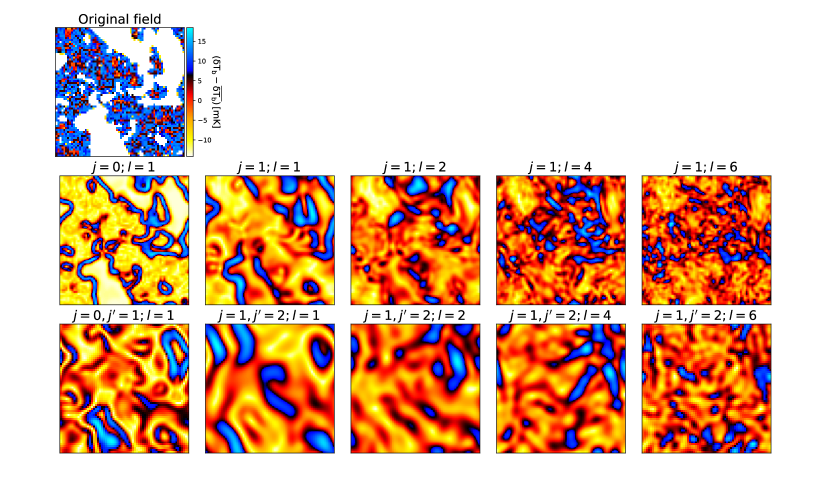
Figure 1 presents the visualization of selected modulus coefficients. Each coefficient reflects some features of the original field. For example, the first-order modulus coefficients with (, ) highlight the boundaries of H II bubbles, while the second-order modulus coefficients with (, , ) show more complex structures. Also, as increases (from the left to right in Figure 1), the modulus coefficients encode the information of small structures of the original field. Note that wavelets with are Gaussian, while wavelets with nonzero can encode rich structures such as filaments.
To compute the scattering coefficients, we choose the maximum scale and maximum angular frequency , and select the value of the modulus power , , or for the first and second-order scattering coefficients. The half-width parameter (i.e. standard deviation in the Gaussian factor) of the mother solid harmonic wavelets is set to be unity, so the maximum scale corresponds to the width of , which matches the number of simulation cells (66 on each side, as will be shown in Section 3.1). For a given (with ) and , the number of the first order coefficients is since takes the value of and the number of the second order coefficients is since and take the value of , ; , ; etc. To keep the dimension of coefficients reasonably low, in this paper, we simply average the information over different for a given . (We will discuss the effect of angular frequencies on the parameter inference in Appendix A.) Therefore, the first and second-order coefficients have a total of components for three values of power , , and .
The zeroth-order coefficient is ill-defined if because the field value at a single pixel can be negative. Also, the zeroth-order coefficient is zero if because it is simply the global sum of the field in this case which is zero for the 21 cm signal by definition (see Section 3.1). Therefore, instead of or , we choose (arbitrarily) three higher modulus power , , and in this paper for the zeroth-order coefficients.
Altogether, the final concatenated coefficient vector has a dimension of , which can be adjusted if necessary. Furthermore, following Allys et al. (2019), we take the logarithms of those coefficients with base 2 as our new coefficients. (If a component is negative, we take the logarithm of the absolute value but keep the sign of the component.) The advantage of adopting these new coefficients is that they behave linearly with and . Hereafter the phrase “scattering coefficients” refers to their logarithms.
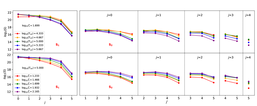
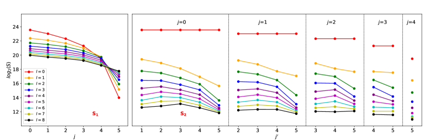
We show the representative values of scattering coefficients in Figure 2. We vary the reionization parameters (see their definitions in Section 3.1), and find that the coefficients are generically suppressed (enhanced) as () increases. This implies that the scattering coefficients are sensitive to the reionization parameters.
2.2 Simulation-based inference with CMAFs
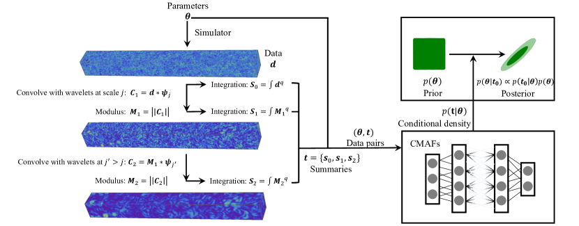
Figure 3 shows the workflow of 3D ScatterNet. The scattering coefficients extracted by the solid harmonic WST serve as the input summaries of the CMAFs444The CMAFs are implemented with pydelfi (Alsing et al. 2019; https://github.com/justinalsing/pydelfi)., which is a variant of the neural density estimators (NDEs) that perform the implicit likelihood inference. We refer interested readers to Paper I for an in-depth description of the DELFI and the CMAFs. The detailed settings of NDEs are given in Appendix D. In this paper, we set two neural layers of a single transform and 50 neurons per layer for CMAFs. We also use the ensembles of CMAFs to improve the performance. The number of transforms and the configuration of ensembles are chosen based on the performance of posterior validation.
2.3 Validation of the posterior
As the final step of inference, we validate both marginalized and joint posteriors. In the posterior validation, hypothesis tests are made to check if the posteriors from CMAFs are self-consistent statistically. Note that the posterior validation is sometimes referred to as “posterior calibration”. However, this step is not to calibrate the trained networks, but simply an indication of whether the network complexity and training data are adequate to learn the conditional density accurately in a statistical manner. We follow Appendix A of Paper I and recap the validation statistics in this subsection.
For the marginalized posterior, the probability integral transform (PIT; Gneiting et al. 2007; Mucesh et al. 2021) is defined as
| (8) |
i.e. the cumulative distribution function (CDF) of the inferred marginal distribution at the true value . If the inferred posteriors are accurate, then the PIT should be uniformly distributed.
For the joint posteriors, there are two statistics. The first one is the copula probability integral transformation (copPIT; Ziegel & Gneiting 2014; Mucesh et al. 2021) which is defined as
| (9) |
Here “Pr” represents the probability and is the CDF of the inferred joint distribution. The copPIT is the multivariate extension of PIT.
The second statistic is the highest probability density (HPD; Harrison et al. 2015) which is defined as
| (10) |
The HPD describes the plausibility of under the distribution . A small value of HPD indicates high plausibility. Similar to the PIT, the copPIT and HPD should be also uniformly distributed if the posteriors are accurate.
In order to check the uniformity, we adopt two metrics, the Kolmogorov-Smirnov (KS; Kolmogorov, 1992) test and Cramér-von Mises (CvM; Anderson, 1962) test, which focus on different aspects of distribution. While the KS test is sensitive to the median, the CvM test captures the tails of a distribution. If the -value from a test is larger than the preset value of significance level, typically 0.01 or 0.05 (Željko Ivezić et al., 2014), then the null hypothesis that these statistics follow a uniform distribution is accepted. Throughout this paper, we adopt the significance level of 0.01 and report the results only if the -value is larger than 0.01 unless stated otherwise.
3 Data preparation
3.1 Cosmic 21 cm Signal
The 21 cm brightness temperature relative to the CMB temperature at position can be written (Furlanetto et al., 2006) as
| (11) |
where in units of mK, is the neutral fraction, and is the matter overdensity, at position . We assume the cold dark matter can be traced by the baryon perturbation on large scales, so . In this paper, we focus on the limit where spin temperature , likely valid soon after reionization begins, though this assumption is strongly model-dependent. As such, we can neglect the dependence on spin temperature. Also, as a demonstration of concept, we ignore the effect of peculiar velocity; such an effect can be readily incorporated in forward simulations by the algorithm introduced by Mao et al. (2012).
In this paper, we use the publicly available code 21cmFAST555https://github.com/andreimesinger/21cmFAST (Mesinger & Furlanetto, 2007; Mesinger et al., 2011), which can be used to perform semi-numerical simulations of reionization, as the simulator to generate the datasets. Our simulations were performed on a cubic box of 100 comoving Mpc on each side, with grid cells. Following the interpolation approach in Paper I, the snapshots at nine different redshifts of the same simulation box (i.e., with the same initial condition) are interpolated to construct a light-cone 21 cm data cube within the comoving distance of a simulation box along the line of sight (LOS). We concatenate 10 such light-cone boxes, each simulated with different initial conditions in density fields but with the same reionization parameters, together to form a full light-cone datacube666We investigate the contributions of individual waveband to parameter inference in Appendix C. of the size comoving (or grid cells) in the redshift range . To mimic the observations from radio interferometers, we subtract from the light-cone field the mean of the 2D slice for each 2D slice perpendicular to the LOS, because radio interferometers cannot measure the mode with .
We parametrize our reionization model as follows, and refer interested readers to Paper I for a detailed explanation of their physical meanings.
(1) , the ionizing efficiency, which is a combination of several parameters related to ionizing photons. In our paper, we vary as .
(2) , the minimum virial temperature of halos that host ionizing sources. In our paper, we vary this parameter as .
Cosmological parameters are fixed in this paper as (, , , , , ) = (0.692, 0.308, 0.0484, 0.968, 0.815, 0.678) (Planck Collaboration et al., 2016).
3.2 Thermal noise and residual foreground
To apply the realistic effects to the 21 cm signal, we first compute the coverage map at each of a total of 660 frequency channels. The coverage map can be used to suppress the thermal noise and calculate the telescope response to the cosmic 21 cm signal and foreground. We then generate the thermal noise with a 1000-hour observation. For the thermal noise estimation in this paper, we employ the Tools21cm777https://github.com/sambit-giri/tools21cm (Giri et al., 2020) code to simulate the expected thermal noise in the 3D 21 cm light-cone images as observed with the SKA1-Low. We list our basic assumptions of the SKA configuration in Table 1. We assume the same telescope response for both the case with thermal noise and that without (i.e. only cosmic 21 cm signal). The signal of a pixel in the space is kept unchanged for non-zero coverage but otherwise set to zero if the pixel is outside the coverage. In order to suppress the noise, we smooth the map with a relatively small baseline of 1 km888Giri et al. (2018); Giri & Mellema (2021); Bianco et al. (2021) choose to smooth with a baseline of 2 km, which corresponds to the size of the central area of SKA1-Low. We discuss the effect of smoothing scales in Appendix B., which roughly corresponds to the size of the core area of SKA1-Low. Specifically, we convolve the map with a Gaussian filter in the angular direction and a top-hat filter in the LOS direction. The FWHM of the Gaussian filter corresponds to the size of the 1-km baseline and the width of the top-hat filter also matches that FWHM.
| Parameters | Values |
|---|---|
| System temperature | |
| Effective collecting area | |
| Integration time | 10 seconds |
| Observation hours per day | 6 hours |
| Total observation time | 1000 hours |
To mock the foreground contamination, we employ the pygsm999https://github.com/telegraphic/pygsm package that is based on the GSM-building model (Zheng et al., 2017), which interpolates the sky maps with 29 sky map observations using an improved principal component analysis (PCA) method. We then use these foreground maps to interpolate our images on the grid for each frequency slice. In order to prevent overfitting, we assign a random patch of sky (except for the North and South poles) to model each foreground image. Finally, we employ the SVD technique for foreground removal. Specifically, we remove the largest six singular value modes.
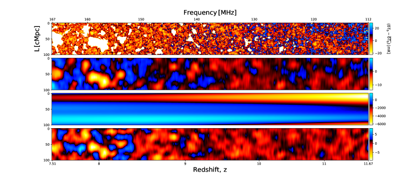
For visualization purposes, we show the mock 21 cm observation with realistic effects in Figure 4. When the cosmic 21 cm signal is applied with the thermal noise of SKA and/or the residual foreground, the features at small scales are washed out but those at the very large scales are still retained.
| Pure signal | SKA noise | SKA noise + residual foreground | ||||||
|---|---|---|---|---|---|---|---|---|
| Parameter | True value | DELFI-3DCNN | 21cmDELFI-PS | 3D ScatterNet | 21cmDELFI-PS | 3D ScatterNet | 21cmDELFI-PS | 3D ScatterNet |
| 4.699 | ||||||||
| 1.477 | ||||||||
| Pure signal | SKA noise | SKA noise + residual foreground | ||||||
|---|---|---|---|---|---|---|---|---|
| Parameter | True value | DELFI-3DCNN | 21cmDELFI-PS | 3D ScatterNet | 21cmDELFI-PS | 3D ScatterNet | 21cmDELFI-PS | 3D ScatterNet |
| 5.477 | ||||||||
| 2.301 | ||||||||
| Pure signal | SKA noise | SKA noise + residual foreground | |||||
| 21cmDELFI-PS | 3D ScatterNet | 21cmDELFI-PS | 3D ScatterNet | 21cmDELFI-PS | 3D ScatterNet | ||
| aafootnotemark: | 0.9989 | 0.9997 | 0.9336 | 0.9647 | 0.7981 | 0.8348 | |
| 0.9978 | 0.9990 | 0.9353 | 0.9604 | 0.8028 | 0.8254 | ||
| bbfootnotemark: | |||||||
| Pure signal | SKA noise | SKA noise + residual foreground | ||||||||||
|---|---|---|---|---|---|---|---|---|---|---|---|---|
| 21cmDELFI-PS | 3D ScatterNet | 21cmDELFI-PS | 3D ScatterNet | 21cmDELFI-PS | 3D ScatterNet | |||||||
| Statistics | KS | CoM | KS | CoM | KS | CoM | KS | CoM | KS | CoM | KS | CoM |
| PIT () | 0.37 | 0.13 | 0.80 | 0.65 | 0.01 | 0.02 | 0.20 | 0.52 | 0.19 | 0.17 | 0.42 | 0.37 |
| PIT () | 0.14 | 0.05 | 0.92 | 0.75 | 0.05 | 0.05 | 0.78 | 0.65 | 0.01 | 0.02 | 0.18 | 0.24 |
| copPIT | 0.54 | 0.39 | 0.67 | 0.92 | 0.01 | 0.03 | 0.64 | 0.85 | 0.53 | 0.31 | 0.46 | 0.46 |
| HPD | 0.04 | 0.01 | 0.63 | 0.48 | 0.01 | 0.01 | 0.41 | 0.47 | 0.74 | 0.67 | 0.05 | 0.03 |
4 Results
For each approach of data compression, we first perform the inference for two representative mock observations — the “Faint Galaxies Model” and the “Bright Galaxies Model”, defined in Tables 2 and 3 (see the “True value” therein), respectively, following the convention of Greig & Mesinger (2017) (see, also, Paper I and Z22b). They are selected as two illustrative examples with extreme parameter values which are nevertheless fine-tuned for these models to have similar global reionization histories. We further perform the posterior validation of the trained NDEs using another set of 300 independent samples that are randomly drawn from the allowed region in the parameter space in which the mean neutral fraction satisfies at , corresponding to the credible region as constrained by the IGM damping wing of ULASJ1120+0641 (Greig et al., 2017).
4.1 3D ScatterNet vs 3D CNN
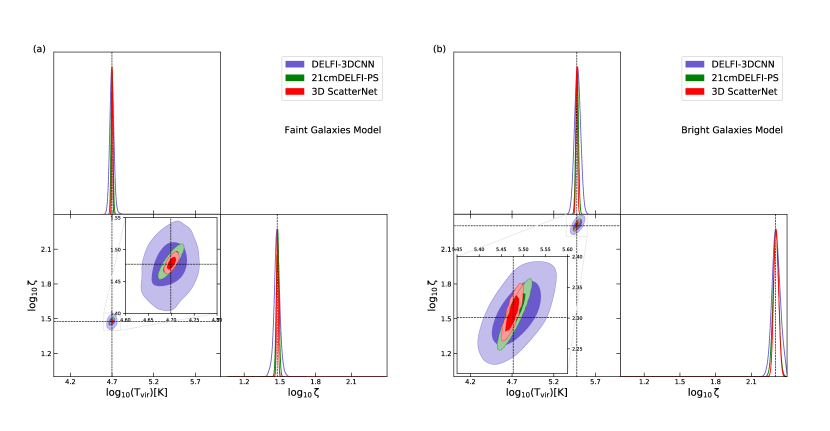
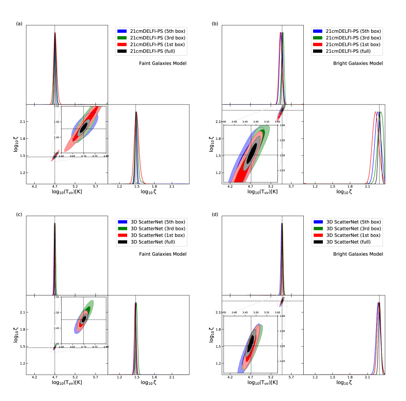
We compare the results using 3D ScatterNet and using DELFI-3D CNN in this subsection. For simplicity, here we only consider the case of cosmological 3D 21 cm images without realistic effect applied except that the mode is removed from each 2D slice perpendicular to the LOS (i.e. “pure signal”). Figure 5 shows the credible regions ( and , or 0.68 and 0.95 levels) for the “Faint Galaxies Model” and the “Bright Galaxies Model”, with quantitative comparisons in terms of medians and (16th and 84th percentile) errors presented in Tables 2 and 3.
The results from DELFI-3DCNN were taken from Paper I, in which the ILI was performed with data compression made by a trained 3D CNN. Paper I used a set of 9,000 samples for training and validation of the 3D CNN and another set of 9,000 samples for training and validation of the density estimators. Nevertheless, if the training sample size was doubled, the results for the “Faint Galaxies Model” and the “Bright Galaxies Model” were not improved, which implies that the inference accuracy might be limited by some intrinsic properties in experimental choices (including the network architecture, characteristics in training datasets, and other hyper-parameter choices) for training the 3D CNN. However, when we replace the data compression from 3D CNN to solid harmonic WST, we find that the inference results are significantly improved in terms of the location and size of credible regions in the posterior distributions for the reionization parameters, as shown in Figure 5 and Tables 2 and 3. Also, the degeneracy of these two parameters is clearly revealed in the credible region for 3D ScatterNet, which indicates that this degeneracy is intrinsic in the theoretical modeling.
Now that the solid harmonic WST represents a better approach to data compression than 3D CNN, we will focus on the 3D ScatterNet in the remainder of this paper.
4.2 3D ScatterNet vs 21cmDELFI-PS
Z22b shows that for the power spectrum analysis, the DELFI approach (i.e. 21cmDELFI-PS) outperforms the standard MCMC analysis. In this subsection, therefore, we compare the results using 3D ScatterNet and 21cmDELFI-PS, both under the same inference strategy using DELFI. On this same footing, we can investigate whether data compression using solid harmonic WST extracts more information from the 3D 21 cm light-cone images than the power spectrum statistic.
4.2.1 Pure Signal
We first consider the “pure signal” case for the comparison, with the credible regions for the “Faint Galaxies Model” and the “Bright Galaxies Model” shown in Figure 5 and quantitative results listed in Tables 2 and 3. For the “Faint Galaxies Model”, the systematic shift (i.e. relative errors of the predicted medians with respect to the true values) and the statistical errors are () for with 3D ScatterNet (21cmDELFI-PS), respectively101010Here for this mock observation, the predicted median with 3D ScatterNet has slightly more deviation (but still within the credible region) from the true value than that with 21cmDELFI-PS. However, testing the medians with 300 samples, we find that the predicted medians using 3D ScatterNet are statistically closer to the true values than those using 21cmDELFI-PS., and () for with 3D ScatterNet (21cmDELFI-PS), respectively. The estimated statistical errors using 3D ScatterNet are about times smaller than using 21cmDELFI-PS. The similar results hold generically for the “Bright Galaxies Model”, too.
Next, we test the trained NDEs on 300 samples. Table 4 shows the coefficient of determination, where and are the true value and the predicted median in a sample for the parameter (e.g. and in this paper), respectively, and the summation is over all testing samples. is the average of the true value over all testing samples. A score of close to unity indicates an overall good inference performance of this parameter. For the case of “pure signal”, both 3D ScatterNet and 21cmDELFI-PS give very high score, but the 3D ScatterNet slightly outperforms the 21cmDELFI-PS.
Table 4 also presents the credible interval of the probability density distribution of , the fractional errors of the deduced parameter in the linear scale (e.g. and in this paper). The fractional error refers to that of the predicted median with respect to the true value, i.e. . For the case of “pure signal”, the typical fractional error (represented by the length of the interval) of 3D ScatterNet is about 1.50 times smaller than that of 21cmDELFI-PS for , and 1.75 times smaller for .
Lastly, we perform the posterior validation. Table 5 shows the -value for some hypothesis tests using 300 testing samples. Note that all -values are larger than 0.01 and most are larger than 0.5, which implies that our results are at least reliable with a significance of 0.01. Also, the -values of 3D ScatterNet are generically larger than those of 21cmDELFI-PS.
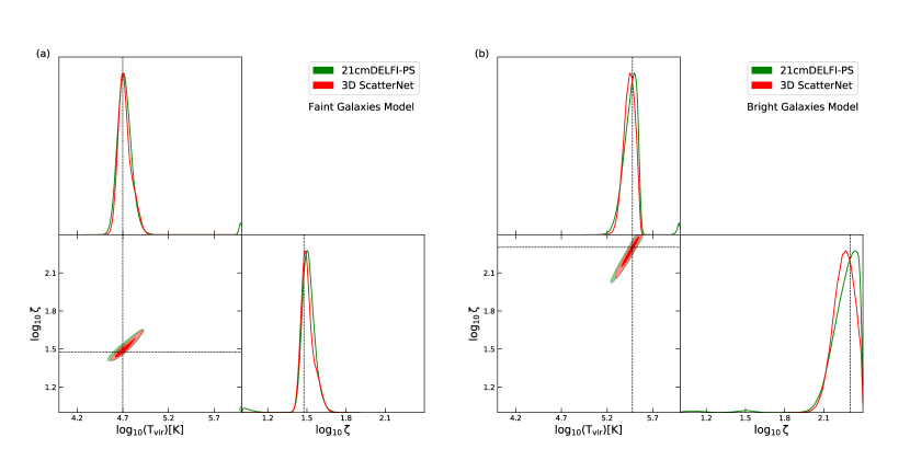
4.2.2 SKA Noise and Residual Foreground
We now consider the case of “SKA noise” which refers to the mock SKA observations of the 3D 21 cm images with total noise (with the contributions from thermal noise and sample variance errors) yet without foreground contamination. Since the images after smoothing with 1-km baseline lose small-scale information, we discard the components of scattering coefficients with and hence the final scattering coefficients have the dimension of 48. For the power spectrum, we also discard the largest -modes in a single box and generate the final power spectrum vector with a dimension of 120.
For the case of “SKA noise”, Figure 6 shows the credible regions for the “Faint Galaxies Model” and the “Bright Galaxies Model”, with quantitative comparisons in terms of medians and errors presented in Tables 2 and 3. The inference results of the “SKA noise” case have larger uncertainties than those of “pure signal”, which is reasonable, given the noise. The statistical errors of 3D ScatterNet are smaller than those of 21cmDELFI-PS. This improvement is also verified by Table 4: the values of 3D ScatterNet are larger than those of 21cmDELFI-PS, and the typical fractional error of the former is about () times smaller for () than that of the latter.
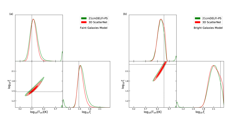
Lastly, we consider the case of “SKA noise + residual foreground” which refers to the mock SKA observations of the 3D 21 cm images with total noise and residual foreground after the foreground is removed with the SVD technique. For the same reason of smoothing as in the “SKA noise” case, we reduce the dimension of the scattering coefficients to be 48 by discarding the components with . For the power spectrum, in order to train reliable NDEs, we have to further discard more large- modes with the upper limit and the final vector of power spectrum has the dimension of 70. In this case, the information for parameter inference is only from large-scale modes because the images are smoothed with a rather coarse resolution.
For the case of “SKA noise + residual foreground”, Figure 7 shows the inference results for two mock observations, with the medians and errors listed in Tables 2 and 3. As expected, given more uncertainties due to residual foreground, the posteriors have larger errors in this case than those of “SKA noise”. The statistical errors of 3D ScatterNet are on average smaller than those of 21cmDELFI-PS. This improvement is also verified by Table 4: the values of 3D ScatterNet are higher than those of 21cmDELFI-PS, and the typical fractional error of the former is about () times smaller for () than that of the latter.
Regarding the posterior validation, all -values are larger than 0.01 both for the “SKA noise” case and the case of “SKA noise + residual foreground”, which implies that our results are at least reliable with a significance of 0.01. Also, the -values of 3D ScatterNet are generically larger than those of 21cmDELFI-PS.
In sum, for all cases of different assumptions in noise and residual foreground, 3D ScatterNet outperforms the 21cmDELFI-PS. Our results demonstrate that the solid harmonic WST can extract the information from the 3D 21 cm light-cone images in a more effective way than the power spectrum statistic itself.
4.3 Discussions
In this subsection, we attempt to provide some insights regarding why the solid harmonic WST outperforms the 3D CNN (trained with the particular set of experimental choices in Paper I) in compressing the 3D 21 cm light-cone images, and the limitations of the 3D CNN configurations in Paper I.
The solid harmonic WST is analogous to a 3D CNN, but unlike the latter, it essentially gives a fixed kernel without the training process. Furthermore, the resulting scattering coefficients are naturally invariant to translations and rotations and are Lipschitz continuous to deformations (Mallat, 2012b). These properties are particularly useful for 3D 21 cm light-cone images because the data summaries have the translational invariance in the angular direction and the rotational invariance along the LOS111111In practice, we obtain approximate invariance that is limited by the boundaries and the discrete sampling of images., and can be stable under slight deformations due to variations in the initial density fields. These intrinsic invariance properties can enhance conditional density learning of the solid harmonic WST.
In principle, thanks to the similarity between solid harmonic WST and 3D CNN, a deep and/or wide 3D CNN should perform at least as well as the WST in extracting information, as long as three conditions are all met — training data is adequate, network is sufficiently expressive, and training process is successful. Our results imply that the 3D CNN configurations in Paper I might have limitations in these three aspects.
The first limitation is insufficient training data. A dataset that samples the complete parameter-data distribution is required to train a robust neural network. For training a 2D CNN (Gillet et al., 2019), a dataset comprising 9,000 training samples might suffice, but the same number of training samples is likely not adequate for 3D CNN. While we find that the results for the “Faint Galaxies Model” and the “Bright Galaxies Model” were not improved if the training sample size was doubled, a thorough scaling test on the number of training samples is necessary to make a robust diagnosis.
The second limitation is the insufficient complexity of neural network architectures. While the solid harmonic WST exploits its intrinsic invariance properties, the standard CNNs cannot because they are not invariant to rotations due to inherent architecture. Thus the architecture in CNNs needs to be fine-tuned during the training. Alternatively, a likely more effective approach is to integrate additional inductive biases into the architecture (Kauderer-Abrams, 2017; Semih Kayhan & van Gemert, 2020; Weiler et al., 2018a, b). In these variants of CNNs, the invariance properties can be enhanced, which might optimize the network architecture.
The third limitation is the sub-optimal network training process. Network optimization involves refined practices for neural network initialization and learning rate determination (DeZoort & Hanin, 2023).
While the 3D CNN configurations in Paper I might be improved in these three aspects, we leave a thorough exploration along these lines to future work.
5 Summary
In this paper, we introduce the solid harmonic WST for compressing the 3D image data and generating meaningful low-dimensional summaries. We apply this technique to the data compression of 3D tomographic 21 cm light-cone images and use the resulting scattering coefficients as the input summaries of the DELFI. With DELFI, we perform the Bayesian inference of the reionization parameters where the likelihood is implicitly defined by the forward simulations. This new technique, dubbed 3D ScatterNet (i.e. solid harmonic WST with DELFI), recovers accurate posterior distributions for the reionization parameters.
We compare the inference results with two different approaches of data compression, the solid harmonic WST and the 3D CNN, for two representative mock observations in the “pure signal” case, and demonstrate that the 3D ScatterNet outperforms the DELFI-3D CNN significantly. Our results imply that the solid harmonic WST extracts the information from the 3D 21 cm light-cone images in a more informative manner than a 3D CNN given reasonable fine-tuning. We also offer insights into enhancing the 3D CNN regarding the datasets, network architecture, and training process. Moreover, the solid harmonic WST has fixed kernels in wavelets, which means that it does not need to be trained in order to output the data summaries. This highlights its robustness and efficiency, which is another advantage of the solid harmonic WST over the 3D CNN.
We then make another comparison of the inference results between data compression using the solid harmonic WST (3D ScatterNet) and using the power spectrum statistic (21cmDELFI-PS), both under the same inference strategy using DELFI. The comparisons were made for three cases with different assumptions on the noise and residual foreground — “pure signal”, “SKA noise” and “SKA noise + residual foreground”. We find that the 3D ScatterNet outperforms the 21cmDELFI-PS in all cases. This implies that the summaries compressed with the solid harmonic WST contain more (i.e. non-Gaussian) information from the 3D 21 cm light-cone images than the power spectrum analysis.
Our results demonstrate that combining a WST (3D solid harmonic WST in this paper) with the simulation-based inference will be a promising tool for the scientific interpretation of future 21 cm light-cone image observation data. Based on the findings of this paper, there is room for improvement with regard to the design of summary statistics from solid harmonic WST or new WST. For example, instead of treating the light-cone as a whole to build a statistic, a variant approach might be to treat discrete boxes separately and concatenate the scattering coefficients of each box together as the data summaries. In this way, the correlations between different stages of reionization can be exploited by the CMAFs. Nevertheless, this will increase the dimension of data summaries and therefore incur higher computational costs, so the trade-off between accuracy and efficiency in the solid harmonic WST is yet to be further explored. Also, further cross-correlation between scales resulting from re-scaling the phase information is likely to be exploited in a 3D extension of the wavelet phase harmonics (WPH; Mallat et al. 2019; Allys et al. 2020) for the 2D case. On the other hand, when scaling the similar analysis to a high-dimensional parameter and/or data space, the diffusion model (Luo, 2022; Legin et al., 2023; Zhao et al., 2023a) is a promising alternative to the CMAFs, or other normalizing flows, to perform the simulation-based inference because of its simplified training objective. We leave the exploration of these directions to future works.
Note. – In the final stage of preparing this manuscript, Greig et al. (2022); Eickenberg et al. (2022) were posted on arXiv. These papers applied the scattering transform (or wavelet moments, varied band-limited first-order scattering coefficients defined in the Fourier space, in Eickenberg et al. 2022) for parameter inference, but both used the Fisher matrix formalism. In comparison, we apply the scattering transform for parameter inference using simulation-based inference in this paper. In addition, Greig et al. (2022) focuses on the reionization parameter estimation using the 2D 21 cm images; Eickenberg et al. (2022) focuses on the cosmological parameter estimation using the 3D cosmological density fields. In comparison, our paper has a distinct focus, i.e. on the reionization parameter estimation using the 3D 21 cm light-cone images.
Acknowledgements
This work is supported by the National SKA Program of China (grant No. 2020SKA0110401), NSFC (grant No. 11821303), and the National Key R&D Program of China (grant No. 2018YFA0404502). BDW acknowledges support from the Simons Foundation. We thank Sihao Cheng, Paulo Montero-Camacho, and Bohua Li for their useful discussions and help. We acknowledge the Tsinghua Astrophysics High-Performance Computing platform at Tsinghua University for providing computational and data storage resources that have contributed to the research results reported within this paper.
Appendix A The effect of angular frequency
In the main text of this paper, the scattering coefficients are averaged over with . In this section, we explore the effect of the angular frequency on the parameter inference.
Figure 8 shows the scattering coefficients evaluated at given values of . While the first-order scattering coefficients show tilting when varying , the second-order scattering coefficients decrease in overall amplitude as increases. Also, for (i.e. Gaussian wavelets), the scattering coefficients are flat at the scale of .
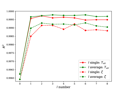
We construct two sets of experiments of posterior inference over 300 testing samples and show the coefficient of determination of the predicted medians in Figure 9. In the first set of experiments (“ single”), the scattering coefficients are evaluated at each single value of . We find that using the information has the smallest values of . When using the information at larger , the value increases and then slightly decreases. This implies that the solid harmonic wavelet has better performance than the Gaussian wavelet (i.e. the case with ). In the second set of experiments (“ average”), the scattering coefficients are averaged over for a given value of . Comparing these two scenarios, we find that the combined information (“ average”) gets a higher value of generically than the single information (“ single”). When increasing the value of , in the case of “ average”, the value increases and then slightly decreases, with the peak at . For this reason, in the main text of this paper, we choose the “ average” scenario with .
Appendix B The effect of smoothing scales
In the main text of this paper, the images are smoothed with the scale corresponding to the size of the 1 km baseline. In this section, we test the effect of smoothing scales on parameter inference. We compute the values of and typical fractional error for the predicted medians of 300 testing samples. Table 6 shows that smoothing with the 1-km baseline has a larger value and smaller fractional error than smoothing with the 2-km baseline. This is because the smoothed images in the former have higher S/N although in coarser resolution. This result is the reason why we chose the size of the 1-km baseline for smoothing in this paper.
| SKA noise | SKA noise + residual foreground | ||||
| 1 km | 2 km | 1 km | 2 km | ||
| 0.9647 | 0.8808 | 0.8348 | 0.7853 | ||
| 0.9604 | 0.9153 | 0.8254 | 0.8212 | ||
| 21cmDELFI-PS | 3D ScatterNet | ||||||||
|---|---|---|---|---|---|---|---|---|---|
| First | Third | Fifth | Full | First | Third | Fifth | Full | ||
| *† | 0.9948 | 0.9863 | 0.9989 | 0.9991 | 0.9987 | 0.9978 | 0.9997 | ||
| * | 0.9909 | 0.9754 | 0.9978 | 0.9960 | 0.9953 | 0.9924 | 0.9990 | ||
| * | |||||||||
| * | |||||||||
Appendix C The dependence of light-cone volumes
In the main text of this paper, the full light-cone images, which concatenate ten light-cone boxes, are exploited for parameter inference. In this section, we investigate whether the information from one of these boxes dominates over the others. (If this were the case, then observations could be optimized targeting at the “sweet-spot” redshift.)
For this purpose, we perform the parameter inference from discrete boxes, both using the power spectrum and using scattering coefficients as summaries. Figure 10 shows the posteriors for two mock observations and Table 7 shows the results of recovery performance for the predicted medians of 300 testing samples. For the 3D ScatterNet, the box at the low-redshift results in better inference performance in terms of larger , smaller typical fractional error, and smaller credible region for mock observations than that at the high-redshift. However, no single box appears to dominate the information, because the full light-cone images always yield the optimal result that is significantly better than any of the single boxes. These results hold similarly for the 21cmDELFI-PS. We conclude that there is no optimal redshift. As such, the full light-cone images, which gather the complete information, provide the parameter inference with the best performance.
Appendix D The NDE setting and sample size
In this section, we give the details of the networks as follows. We choose the MAFs as the NDEs throughout of this paper. In all architectures, we set two neural layers of a single transform with 50 neurons per layer. We also use the ensembles of NDEs. The final posterior is the stacked one from individual posteriors with weights according to their training errors. We fine-tune the training sample size and the CMAFs architecture for every method and experiment based on the outcomes of posterior validation (calibration). The guiding principle behind this fine-tuning is that data (summaries) with greater uncertainties might require more intricate CMAFs, such as increased transformations within a single CMAF. Meanwhile, data (summaries) of higher dimensions might necessitate a more substantial training sample due to the vast feature space.
The procedure for scattering coefficients is as follows.
-
(1)
The scattering coefficients for the “pure signal” case with mode removed. We use 18,000 light-cone images and an ensemble of 8 NDEs , which means that we have two NDE blocks, each having the NDE with the number of transformations 5, 6, 7, and 8, respectively. Hereafter we use the same terminology. Notice that the final performance can be further enhanced with double the size of the light-cone images. To fairly compare with 21cmDELFI-PS, we use 18,000 images for reports in the paper.
-
(2)
We use 36,000 light-cone images and the coefficients from pure discrete boxes. We use 27,000 samples. The ensembles for the first, third, and fifth boxes: , , , respectively.
-
(3)
We use 36,000 light-cone images and the coefficients with the information of averaged from pure boxes. The ensembles from to : , , , , , , , , respectively.
-
(4)
The coefficients with the information of single from pure boxes. The ensembles from to : , , , , , , , , , respectively.
-
(5)
The coefficients from the signal with SKA noise. We use 27,000 samples. The ensembles for the signal with 1-km smoothing: , and 2-km smoothing: , respectively.
-
(6)
The coefficients from the signal with SKA noise and residual foreground. The ensembles for the signal with 1-km smoothing: , and 2-km smoothing: , respectively.
The procedure for the power spectrum is as follows.
-
(1)
The power spectrum from pure signal with mode removed. We use 18,000 samples and the ensembles .
-
(2)
The power spectrum from pure discrete boxes. For the first box, we use 32,596 samples and the ensembles ; for the third box, we use 34,044 samples and the ensembles ; and for the fifth box, we use 27,000 samples and the ensembles .
-
(3)
The power spectrum from the signal with SKA noise. We use 27,000 samples and the ensembles .
-
(4)
The power spectrum from the signal with SKA noise and residual foreground. We use 36,000 samples and the ensembles .
References
- Abadi et al. (2016) Abadi, M., Barham, P., Chen, J., et al. 2016, in Proceedings of the 12th USENIX Conference on Operating Systems Design and Implementation, OSDI’16 (Berkeley, CA: USENIX Association), 265–283
- Abdurashidova et al. (2022) Abdurashidova, Z., Aguirre, J. E., Alexander, P., et al. 2022, ApJ, 925, 221, doi: 10.3847/1538-4357/ac1c78
- Allys et al. (2019) Allys, E., Levrier, F., Zhang, S., et al. 2019, A&A, 629, A115, doi: 10.1051/0004-6361/201834975
- Allys et al. (2020) Allys, E., Marchand, T., Cardoso, J. F., et al. 2020, Phys. Rev. D, 102, 103506, doi: 10.1103/PhysRevD.102.103506
- Alsing et al. (2019) Alsing, J., Charnock, T., Feeney, S., & Wandelt, B. 2019, MNRAS, 488, 4440, doi: 10.1093/mnras/stz1960
- Alsing et al. (2018) Alsing, J., Wandelt, B., & Feeney, S. 2018, MNRAS, 477, 2874, doi: 10.1093/mnras/sty819
- Anderson (1962) Anderson, T. W. 1962, The Annals of Mathematical Statistics, 33, 1148 , doi: 10.1214/aoms/1177704477
- Andreux et al. (2018) Andreux, M., Angles, T., Exarchakis, G., et al. 2018, arXiv e-prints, arXiv:1812.11214. https://arxiv.org/abs/1812.11214
- Astropy Collaboration et al. (2013) Astropy Collaboration, Robitaille, T. P., Tollerud, E. J., et al. 2013, A&A, 558, A33, doi: 10.1051/0004-6361/201322068
- Astropy Collaboration et al. (2018) Astropy Collaboration, Price-Whelan, A. M., Sipőcz, B. M., et al. 2018, AJ, 156, 123, doi: 10.3847/1538-3881/aabc4f
- Bianco et al. (2021) Bianco, M., Giri, S. K., Iliev, I. T., & Mellema, G. 2021, Monthly Notices of the Royal Astronomical Society, 505, 3982, doi: 10.1093/mnras/stab1518
- Cheng et al. (2020) Cheng, S., Ting, Y.-S., Ménard, B., & Bruna, J. 2020, MNRAS, 499, 5902, doi: 10.1093/mnras/staa3165
- Chung (2022) Chung, D. T. 2022, MNRAS, 517, 1625, doi: 10.1093/mnras/stac2662
- Cranmer et al. (2020) Cranmer, K., Brehmer, J., & Louppe, G. 2020, Proceedings of the National Academy of Sciences, 117, 30055, doi: 10.1073/pnas.1912789117
- de Oliveira-Costa et al. (2008) de Oliveira-Costa, A., Tegmark, M., Gaensler, B. M., et al. 2008, MNRAS, 388, 247, doi: 10.1111/j.1365-2966.2008.13376.x
- DeBoer et al. (2017) DeBoer, D. R., Parsons, A. R., Aguirre, J. E., et al. 2017, Publications of the Astronomical Society of the Pacific, 129, 045001. http://stacks.iop.org/1538-3873/129/i=974/a=045001
- DeZoort & Hanin (2023) DeZoort, G., & Hanin, B. 2023, arXiv e-prints, arXiv:2306.11668, doi: 10.48550/arXiv.2306.11668
- Eickenberg et al. (2017) Eickenberg, M., Exarchakis, G., Hirn, M., & Mallat, S. 2017, in Proceedings of the 31st International Conference on Neural Information Processing Systems, NIPS’17 (Red Hook, NY, USA: Curran Associates Inc.), 6543–6552
- Eickenberg et al. (2018) Eickenberg, M., Exarchakis, G., Hirn, M., Mallat, S., & Thiry, L. 2018, The Journal of chemical physics, 148, 241732
- Eickenberg et al. (2022) Eickenberg, M., Allys, E., Moradinezhad Dizgah, A., et al. 2022, arXiv e-prints, arXiv:2204.07646, doi: 10.48550/arXiv.2204.07646
- Furlanetto et al. (2006) Furlanetto, S. R., Oh, S. P., & Briggs, F. H. 2006, Physics Reports, 433, 181, doi: 10.1016/j.physrep.2006.08.002
- Gauthier et al. (2021) Gauthier, S., Thérien, B., Alsène-Racicot, L., et al. 2021, arXiv e-prints, arXiv:2107.09539, doi: 10.48550/arXiv.2107.09539
- Gillet et al. (2019) Gillet, N., Mesinger, A., Greig, B., Liu, A., & Ucci, G. 2019, MNRAS, 484, 282, doi: 10.1093/mnras/stz010
- Giri & Mellema (2021) Giri, S. K., & Mellema, G. 2021, MNRAS, 505, 1863, doi: 10.1093/mnras/stab1320
- Giri et al. (2018) Giri, S. K., Mellema, G., & Ghara, R. 2018, MNRAS, 479, 5596, doi: 10.1093/mnras/sty1786
- Giri et al. (2020) Giri, S. K., Mellema, G., & Jensen, H. 2020, Journal of Open Source Software, 5, 2363, doi: 10.21105/joss.02363
- Gneiting et al. (2007) Gneiting, T., Balabdaoui, F., & Raftery, A. E. 2007, Journal of the Royal Statistical Society: Series B (Statistical Methodology), 69, 243, doi: https://doi.org/10.1111/j.1467-9868.2007.00587.x
- Górski et al. (2005) Górski, K. M., Hivon, E., Banday, A. J., et al. 2005, ApJ, 622, 759, doi: 10.1086/427976
- Greig & Mesinger (2015) Greig, B., & Mesinger, A. 2015, MNRAS, 449, 4246, doi: 10.1093/mnras/stv571
- Greig & Mesinger (2017) —. 2017, MNRAS, 472, 2651, doi: 10.1093/mnras/stx2118
- Greig & Mesinger (2018) —. 2018, MNRAS, 477, 3217, doi: 10.1093/mnras/sty796
- Greig et al. (2017) Greig, B., Mesinger, A., Haiman, Z., & Simcoe, R. A. 2017, MNRAS, 466, 4239, doi: 10.1093/mnras/stw3351
- Greig et al. (2022) Greig, B., Ting, Y.-S., & Kaurov, A. A. 2022, arXiv e-prints, arXiv:2204.02544. https://arxiv.org/abs/2204.02544
- Harris et al. (2020) Harris, C. R., Millman, K. J., van der Walt, S. J., et al. 2020, Nature, 585, 357, doi: 10.1038/s41586-020-2649-2
- Harrison et al. (2015) Harrison, D., Sutton, D., Carvalho, P., & Hobson, M. 2015, MNRAS, 451, 2610, doi: 10.1093/mnras/stv1110
- Hunter (2007) Hunter, J. D. 2007, Computing in Science & Engineering, 9, 90, doi: 10.1109/MCSE.2007.55
- Intema et al. (2017) Intema, H. T., Jagannathan, P., Mooley, K. P., & Frail, D. A. 2017, A&A, 598, A78, doi: 10.1051/0004-6361/201628536
- Jacobs et al. (2015) Jacobs, D. C., Pober, J. C., Parsons, A. R., et al. 2015, ApJ, 801, 51, doi: 10.1088/0004-637X/801/1/51
- Jeffrey et al. (2022) Jeffrey, N., Boulanger, F., Wandelt, B. D., et al. 2022, MNRAS, 510, L1, doi: 10.1093/mnrasl/slab120
- Kauderer-Abrams (2017) Kauderer-Abrams, E. 2017, arXiv e-prints, arXiv:1801.01450. https://arxiv.org/abs/1801.01450
- Kolmogorov (1992) Kolmogorov, A. 1992, On the Empirical Determination of a Distribution Function, ed. S. Kotz & N. L. Johnson (New York, NY: Springer New York), 106–113, doi: 10.1007/978-1-4612-4380-9_10
- Legin et al. (2023) Legin, R., Ho, M., Lemos, P., et al. 2023, arXiv e-prints, arXiv:2304.03788, doi: 10.48550/arXiv.2304.03788
- Lewis (2019) Lewis, A. 2019. https://arxiv.org/abs/1910.13970
- Luo (2022) Luo, C. 2022, arXiv e-prints, arXiv:2208.11970, doi: 10.48550/arXiv.2208.11970
- Mallat (2012a) Mallat, S. 2012a, Communications on Pure and Applied Mathematics, 65, 1331, doi: https://doi.org/10.1002/cpa.21413
- Mallat (2012b) —. 2012b, Communications on Pure and Applied Mathematics, 65, 1331, doi: https://doi.org/10.1002/cpa.21413
- Mallat et al. (2019) Mallat, S., Zhang, S., & Rochette, G. 2019, Information and Inference: A Journal of the IMA, 9, 721, doi: 10.1093/imaiai/iaz019
- Mao et al. (2012) Mao, Y., Shapiro, P. R., Mellema, G., et al. 2012, MNRAS, 422, 926, doi: 10.1111/j.1365-2966.2012.20471.x
- Masui et al. (2013) Masui, K. W., Switzer, E. R., Banavar, N., et al. 2013, ApJ, 763, L20, doi: 10.1088/2041-8205/763/1/L20
- Mellema et al. (2013) Mellema, G., Koopmans, L. V. E., Abdalla, F. A., et al. 2013, Experimental Astronomy, 36, 235, doi: 10.1007/s10686-013-9334-5
- Mertens et al. (2020) Mertens, F. G., Mevius, M., Koopmans, L. V. E., et al. 2020, MNRAS, 493, 1662, doi: 10.1093/mnras/staa327
- Mesinger & Furlanetto (2007) Mesinger, A., & Furlanetto, S. 2007, ApJ, 669, 663, doi: 10.1086/521806
- Mesinger et al. (2011) Mesinger, A., Furlanetto, S., & Cen, R. 2011, MNRAS, 411, 955, doi: 10.1111/j.1365-2966.2010.17731.x
- Mucesh et al. (2021) Mucesh, S., Hartley, W. G., Palmese, A., et al. 2021, MNRAS, 502, 2770, doi: 10.1093/mnras/stab164
- Neutsch et al. (2022) Neutsch, S., Heneka, C., & Brüggen, M. 2022, MNRAS, 511, 3446, doi: 10.1093/mnras/stac218
- Paciga et al. (2013) Paciga, G., Albert, J. G., Bandura, K., et al. 2013, MNRAS, 433, 639, doi: 10.1093/mnras/stt753
- Papamakarios (2019) Papamakarios, G. 2019, arXiv e-prints, arXiv:1910.13233. https://arxiv.org/abs/1910.13233
- Papamakarios et al. (2021) Papamakarios, G., Nalisnick, E., Rezende, D. J., Mohamed, S., & Lakshminarayanan, B. 2021, Journal of Machine Learning Research, 22, 1. http://jmlr.org/papers/v22/19-1028.html
- Papamakarios et al. (2017) Papamakarios, G., Pavlakou, T., & Murray, I. 2017, in Proceedings of the 31st International Conference on Neural Information Processing Systems, NIPS’17 (Red Hook, NY, USA: Curran Associates Inc.), 2335
- Parsons et al. (2010) Parsons, A. R., Backer, D. C., Foster, G. S., et al. 2010, ApJ, 139, 1468. http://stacks.iop.org/1538-3881/139/i=4/a=1468
- Parsons et al. (2014) Parsons, A. R., Liu, A., Aguirre, J. E., et al. 2014, The Astrophysical Journal, 788, 106, doi: 10.1088/0004-637X/788/2/106
- Pedersen et al. (2022) Pedersen, C., Ho, S., & Eickenberg, M. 2022, in Machine Learning for Astrophysics, 40
- Pedregosa et al. (2011) Pedregosa, F., Varoquaux, G., Gramfort, A., et al. 2011, Journal of Machine Learning Research, 12, 2825
- Planck Collaboration et al. (2016) Planck Collaboration, Ade, P. A. R., Aghanim, N., et al. 2016, A&A, 594, A13, doi: 10.1051/0004-6361/201525830
- Prelogović & Mesinger (2023) Prelogović, D., & Mesinger, A. 2023, arXiv e-prints, arXiv:2305.03074, doi: 10.48550/arXiv.2305.03074
- Prelogović et al. (2022) Prelogović, D., Mesinger, A., Murray, S., Fiameni, G., & Gillet, N. 2022, MNRAS, 509, 3852, doi: 10.1093/mnras/stab3215
- Ramachandran & Varoquaux (2011) Ramachandran, P., & Varoquaux, G. 2011, Computing in Science and Engg., 13, 40–51, doi: 10.1109/MCSE.2011.35
- Saydjari et al. (2021) Saydjari, A. K., Portillo, S. K. N., Slepian, Z., et al. 2021, ApJ, 910, 122, doi: 10.3847/1538-4357/abe46d
- Semih Kayhan & van Gemert (2020) Semih Kayhan, O., & van Gemert, J. C. 2020, in 2020 IEEE/CVF Conference on Computer Vision and Pattern Recognition (CVPR) (Piscataway, NJ: IEEE), 14262, doi: 10.1109/CVPR42600.2020.01428
- Stewart (1993) Stewart, G. W. 1993, SIAM Rev., 35, 551–566, doi: 10.1137/1035134
- Tejero-Cantero et al. (2020) Tejero-Cantero, A., Boelts, J., Deistler, M., et al. 2020, Journal of Open Source Software, 5, 2505, doi: 10.21105/joss.02505
- Tingay et al. (2013) Tingay, S. J., Goeke, R., Bowman, J. D., et al. 2013, Publications of the Astronomical Society of Australia, 30, e007, doi: 10.1017/pasa.2012.007
- Trott (2016) Trott, C. M. 2016, MNRAS, 461, 126, doi: 10.1093/mnras/stw1310
- Trott et al. (2020) Trott, C. M., Jordan, C. H., Midgley, S., et al. 2020, MNRAS, 493, 4711, doi: 10.1093/mnras/staa414
- Valogiannis & Dvorkin (2022) Valogiannis, G., & Dvorkin, C. 2022, Phys. Rev. D, 105, 103534, doi: 10.1103/PhysRevD.105.103534
- van Haarlem et al. (2013) van Haarlem, M. P., Wise, M. W., Gunst, A. W., et al. 2013, A&A, 556, A2, doi: 10.1051/0004-6361/201220873
- Van Rossum & Drake (2009) Van Rossum, G., & Drake, F. L. 2009, Python 3 Reference Manual (Scotts Valley, CA: CreateSpace)
- Van Rossum & Drake Jr (1995) Van Rossum, G., & Drake Jr, F. L. 1995, Python reference manual (Centrum voor Wiskunde en Informatica Amsterdam)
- Virtanen et al. (2020) Virtanen, P., Gommers, R., Oliphant, T. E., et al. 2020, Nature Methods, 17, 261, doi: 10.1038/s41592-019-0686-2
- Waskom (2021) Waskom, M. L. 2021, Journal of Open Source Software, 6, 3021, doi: 10.21105/joss.03021
- Weiler et al. (2018a) Weiler, M., Geiger, M., Welling, M., Boomsma, W., & Cohen, T. S. 2018a, in Advances in Neural Information Processing Systems, ed. S. Bengio, H. Wallach, H. Larochelle, K. Grauman, N. Cesa-Bianchi, & R. Garnett, Vol. 31 (Curran Associates, Inc.). https://proceedings.neurips.cc/paper_files/paper/2018/file/488e4104520c6aab692863cc1dba45af-Paper.pdf
- Weiler et al. (2018b) Weiler, M., Hamprecht, F. A., & Storath, M. 2018b, in 2018 IEEE/CVF Conference on Computer Vision and Pattern Recognition, 849–858, doi: 10.1109/CVPR.2018.00095
- Wolz et al. (2015) Wolz, L., Abdalla, F. B., Alonso, D., et al. 2015, PoS, AASKA14, 035, doi: 10.22323/1.215.0035
- Yoshiura et al. (2021) Yoshiura, S., Pindor, B., Line, J. L. B., et al. 2021, MNRAS, 505, 4775, doi: 10.1093/mnras/stab1560
- Zhao et al. (2022a) Zhao, X., Mao, Y., Cheng, C., & Wandelt, B. D. 2022a, ApJ, 926, 151, doi: 10.3847/1538-4357/ac457d
- Zhao et al. (2022b) Zhao, X., Mao, Y., & Wandelt, B. D. 2022b, arXiv e-prints, arXiv:2203.15734. https://arxiv.org/abs/2203.15734
- Zhao et al. (2023a) Zhao, X., Ting, Y.-S., Diao, K., & Mao, Y. 2023a, MNRAS, 526, 1699, doi: 10.1093/mnras/stad2778
- Zhao et al. (2023b) Zhao, X., Zuo, S., & Mao, Y. 2023b, arXiv e-prints, arXiv:2307.09530, doi: 10.48550/arXiv.2307.09530
- Zheng et al. (2017) Zheng, H., Tegmark, M., Dillon, J. S., et al. 2017, MNRAS, 464, 3486, doi: 10.1093/mnras/stw2525
- Ziegel & Gneiting (2014) Ziegel, J. F., & Gneiting, T. 2014, Electronic Journal of Statistics, 8, 2619 , doi: 10.1214/14-EJS964
- Zonca et al. (2019) Zonca, A., Singer, L., Lenz, D., et al. 2019, Journal of Open Source Software, 4, 1298, doi: 10.21105/joss.01298
- Željko Ivezić et al. (2014) Željko Ivezić, Connolly, A. J., VanderPlas, J. T., & Gray, A. 2014, Statistics, Data Mining, and Machine Learning in Astronomy: A Practical Python Guide for the Analysis of Survey Data (Princeton University Press), doi: doi:10.1515/9781400848911