SPA: A Graph Spectral Alignment Perspective for
Domain Adaptation

Abstract

Unsupervised domain adaptation (UDA) is a pivotal form in machine learning to extend the in-domain model to the distinctive target domains where the data distributions differ. Most prior works focus on capturing the inter-domain transferability but largely overlook rich intra-domain structures, which empirically results in even worse discriminability. In this work, we introduce a novel graph SPectral Alignment (SPA) framework to tackle the tradeoff. The core of our method is briefly condensed as follows: (i)-by casting the DA problem to graph primitives, SPA composes a coarse graph alignment mechanism with a novel spectral regularizer towards aligning the domain graphs in eigenspaces; (ii)-we further develop a fine-grained message propagation module — upon a novel neighbor-aware self-training mechanism — in order for enhanced discriminability in the target domain. On standardized benchmarks, the extensive experiments of SPA demonstrate that its performance has surpassed the existing cutting-edge DA methods. Coupled with dense model analysis, we conclude that our approach indeed possesses superior efficacy, robustness, discriminability, and transferability. Code and data are available at: https://github.com/CrownX/SPA.

1 Introduction

Domain adaptation (DA) problem is a widely studied area in computer vision field [20, 19, 73, 65, 40], which aims to transfer knowledge from label-rich source domains to label-scare target domains where dataset shift [32] or domain shift [72] exists. The existing unsupervised domain adaptation (UDA) methods usually explore the idea of learning domain-invariant feature representations based on the theoretical analysis [3]. These methods can be generally categorized several types, i.e., moment matching methods [44, 51, 70], and adversarial learning methods [18, 66, 19, 52].

The most essential challenge of domain adaptation is how to find a suitable utilization of intra-domain information and inter-domain information to properly align target samples. More specifically, it is a trade-off between discriminating data samples of different categories within a domain to the greatest extent possible, and learning transferable features across domains with the existence of domain shift. To achieve this, adversarial learning methods implicitly mitigate the domain shift by driving the feature extractor to extract indistinguishable features and fool the domain classifier. The adversarial DA methods have been increasingly developed and followed by a series of works [14, 45, 8]. However, it is very unexpected that the remarkable transferability of DANN [18] is enhanced at the expense of worse discriminability [10, 38].

To mitigate this problem, there is a promising line of studies that explore graph-based UDA algorithms [9, 87, 54]. The core idea is to establish correlation graphs within domains and leverage the rich topological information to connect inter-domain samples and decrease their distances. In this way, self-correlation graphs with intra-domain information are constructed, which exhibits the homophily property whereby nearby samples tend to receive similar predictions [55]. There comes the problem that is how to transfer the inter-domain information with these rich topological information. Graph matching is a direct solution to inter-domain alignment problems. Explicit graph matching methods are usually designed to find sample-to-sample mapping relations, requiring multiple matching stages for nodes and edges respectively [9], or complicated structure mapping with an attention matrix [54]. Despite the promise, we find that such a point-wise matching strategy can be restrictive and inflexible. In effect, UDA does not require an exact mapping plan from one node to another one in different domains. Its expectation is to align the entire feature space such that label information of source domains can be transferred and utilized in target domains.

In this work, we introduce a novel graph spectral alignment perspective for UDA, hierarchically solving the aforementioned problem. In a nutshell, our method encapsulates a coarse graph alignment module and a fine-grained message propagation module, jointly balancing inter-domain transferability and intra-domain discriminability. Core to our method, we propose a novel spectral regularizer that projects domain graphs into eigenspaces and aligns them based on their eigenvalues. This gives rise to coarse-grained topological structures transfer across domains but in a more intrinsic way than restrictive point-wise matching. Thereafter, we perform the fine-grained message passing in the target domain via a neighbor-aware self-training mechanism. By then, our algorithm is able to refine the transferred topological structure to produce a discriminative domain classifier.

We conduct extensive evaluations on several benchmark datasets including DomainNet, OfficeHome, Office31, and VisDA2017. The exprimental results show that our method consistently outperforms existing state-of-the-art domain adaptation methods, improving the accuracy on 8.6% on original DomainNet dataset and about 2.6% on OfficeHome dataset. Furthermore, the comprehensive model analysis demonstrates the the superiority of our method in efficacy, robustness, discriminability and transferability.

2 Preliminaries

Problem Description. Given source domain data $\mathcal{D}_{s}=\left\{\left(x_{i}^{s},y_{i}^{s}\right)\right\}_{i=1}^{N_{s}}$ of $N_{s}$ labeled samples associated with $C_{s}$ categories from $\mathcal{X}_{s}\times\mathcal{Y}_{s}$ and target domain data $\mathcal{D}_{t}=\left\{x_{i}^{t}\right\}_{i=1}^{N_{t}}$ of $N_{t}$ unlabeled samples associated with $C_{t}$ categories from $\mathcal{X}_{t}$. We assume that the domains share the same feature and label space but follow different marginal data distributions, following the Covariate Shift [67]; that is, $P\left(\mathcal{X}_{s}\right)\neq P\left(\mathcal{X}_{t}\right)$ but $P\left(\mathcal{Y}_{s}\mid\mathcal{X}_{s}\right)=P\left(\mathcal{Y}_{t}\mid\mathcal{X}_{t}\right)$. Domain adaptation just occurs when the underlying distributions corresponding to the source and target domains in the shared label space are different but similar enough to make sense the transfer [15]. The goal of unsupervised domain adaptation is to predict the label $\left\{y_{i}^{t}\right\}_{i=1}^{N_{t}}$ in the target domain, where $y_{i}^{t}\in\mathcal{Y}_{t}$, and the source task is $\mathcal{X}_{s}\rightarrow\mathcal{Y}_{s}$ assumed to be the same with the target task $\mathcal{X}_{t}\rightarrow\mathcal{Y}_{t}$.

Adversarial Domain Adaptation. The family of adversarial domain adaptation methods, e.g., Domain Adversarial Neural Network (DANN) [18] have become significantly influential in domain adaptation. The fundamental idea behind is to learn transferable features that explicitly reduce the domain shift. Similar to standard supervised classification methods, these approaches include a feature extractor $F(\cdot)$ and a category classifier $C(\cdot)$. Additionally, a domain classifier $D(\cdot)$ is trained to distinguish the source domain from the target domain and meanwhile the feature extractor $F(\cdot)$ is trained to confuse the domain classifier and learn domain-invariant features. The supervised classification loss $\mathcal{L}_{cls}$ and domain adversarial loss $\mathcal{L}_{adv}$ are presented as bellow:

$$\begin{split}\mathcal{L}_{cls}&=\mathbb{E}_{\left(x_{i}^{s},y_{i}^{s}\right)\sim\mathcal{D}_{\mathcal{S}}}\mathcal{L}_{ce}\left(C\left(F\left(x_{i}^{s}\right)\right),y_{i}^{s}\right)\\ \mathcal{L}_{adv}&=\mathbb{E}_{F\left(x_{i}^{s}\right)\sim\tilde{\mathcal{D}}_{s}}\log\left[D\left(F\left(x_{i}^{s}\right)\right)\right]\\ &+\mathbb{E}_{F\left(x_{i}^{t}\right)\sim\tilde{\mathcal{D}}_{t}}\log\left[1-D\left(F\left(x_{i}^{t}\right)\right)\right]\end{split}$$ (1)

where $\tilde{\mathcal{D}}_{s}$ and $\tilde{\mathcal{D}}_{t}$ denote the induced feature distributions of $\mathcal{D}_{s}$ and $\mathcal{D}_{t}$ respectively, and $\mathcal{L}_{ce}(\cdot,\cdot)$ is the cross-entropy loss function.

3 Methodology

In this section, we will give a specific introduction to our approach. The overall pipeline is shown in Figure 1. Our method is able to effectively utilize both intra-domain and inter-domain relations simultaneously for domain adaptation tasks. Specifically, based on our constructed dynamic graphs in Section 3.1, we propose a novel framework that utilizes graph spectra to align inter-domain relations in Section 3.2, and leverages intra-domain relations via neighbor-aware propagation mechanism in Section 3.3. Our approach enables us to effectively capture the underlying domain distributions while ensuring that the learned features are transferable across domains.

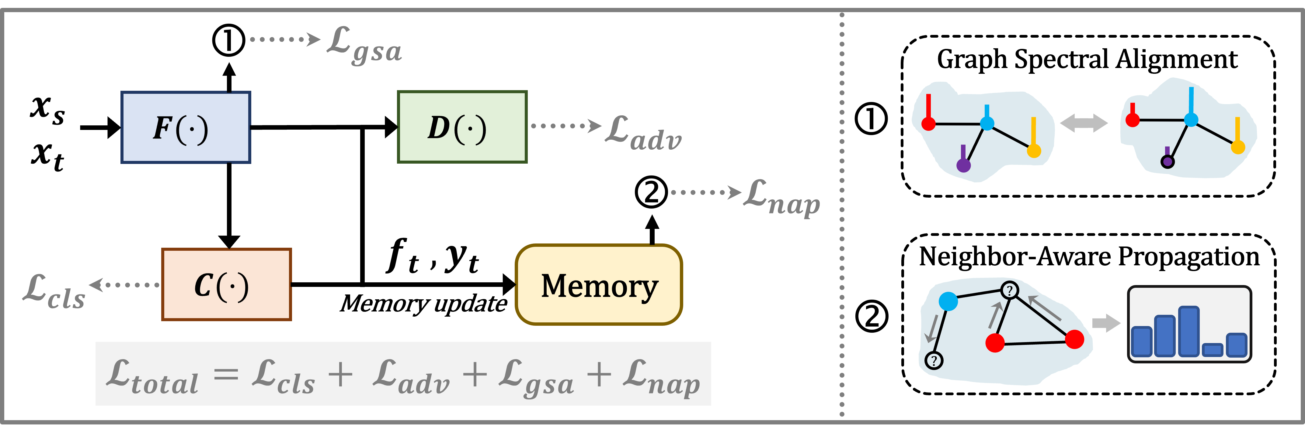
Figure 1: The overall architecture. The final objective integrates supervised classification loss $\mathcal{L}_{cls}$, domain adversarial loss $\mathcal{L}_{adv}$, neighbor-aware propagation loss $\mathcal{L}_{nap}$, and graph spectral alignment loss $\mathcal{L}_{spa}$.

3.1 Dynamic Graph Construction

Images and text data inherently contain rich sequential or spatial structures that can be effectively represented using graphs. By constructing graphs based on the data, both intra-domain relations and inter-domain relations can be exploited. For instance, semantic and spatial relations among detected objects in an image [43], cross-modal relations among images and sentences [11], cross-domain relations among images and texts [9, 27] have been successfully modeled using graph-based representations. In this paper, leveraging self-correlation graphs enables us to model the relations between different samples within domain and capture the underlying data distributions.

Our self-correlation graphs are constructed on source features and target features respectively. A feature extractor $F(\cdot)$ can be designed to learn source features $f_{s}$ and target features $f_{t}$ from source domain samples $\mathbf{x}_{s}$ and target domain samples $\mathbf{x}_{t}$ respectively, i.e., $f_{s}=F(x_{s})$ and $f_{t}=F(x_{t})$. Given the extracted features $f_{s}$, we aim to construct a undirected and weighted graph $\mathcal{G}_{s}=(\mathcal{V}_{s},\mathcal{E}_{s})$. Each vertex $v_{i}\in\mathcal{V}_{s}$ is represented by a feature vector $f_{i}^{s}$. Each weighted edge $e_{i,j}\in\mathcal{E}_{s}$ can be formulated as a relation between a pair of entities $\delta(f_{i}^{s},f_{j}^{s})$, where $\delta(\cdot)$ denotes a metric function. With the extracted features $f_{t}$, another graph $\mathcal{G}_{s}=(\mathcal{V}_{t},\mathcal{E}_{t})$ can be constructed in the same way. Note that both $f_{s}$ and $f_{t}$ keep evolving along with the update of parameter $\theta$ during the training process. Their adjacency matrices are denoted as $\mathbf{A}_{s}$ and $\mathbf{A}_{t}$ respectively. As is well-known, the adjacency matrix of a graph contains all of its topological information. By representing these graphs in domain adaptation tasks, we can directly obtain the intra-domain relations and regard inter-domain alignment as a graph matching problem [9].

3.2 Graph Spectral Alignment

In this section, we will introduce how to align inter-domain relations for source domain graphs and target domain graphs. In domain adaptation scenarios where domain shift exits, if we directly construct a graph with source and target domain features together, we can only obtain a graph beyond the homophily assumption. In this way, a necessary domain alignment comes out.

As stated in Section 3.1, based on our correlation graphs, the inter-domain alignment can be regard as a graph matching problem. Explicit graph matching methods aim to find a one-to-one correspondence between nodes or edges of two graphs and typically involve solving a combinatorial optimization problem for node matching and edge matching respectively [9]. Nevertheless, our goal is often to align the distributions of the source and target domains and learn domain-invariant features, instead of requiring such an complicated matching approach. Therefore, we prefer a implicit graph alignment method, avoiding multiple stages of explicit graph matching.

The distance between the spectra of graphs is able to measure how far apart the spectrum of a graph with $n$ vertices can be from the spectrum of any other graph with $n$ vertices [1, 69, 22], leading to a simplification of measuring the discrepancy of graphs. Inspired by this, we give the definitions of graph laplacians and spectral distances:

Definition 1.

(Graph Laplacians [77]). Let $\mathcal{G}=(\mathcal{V},\mathcal{E})$ be a finite graph with vertices $\mathcal{V}$ and weighted edges $\mathcal{E}$. Let $\phi:\mathcal{V}\rightarrow\mathcal{R}$ be a function of the vertices taking values in a ring and $\gamma:\mathcal{E}\rightarrow\mathcal{R}$ be a weighting function of weighed edges. Then, the graph Laplacian $\Delta$ acting on $\phi$ and $\gamma$ is defined by

$$(\Delta_{\gamma}\phi)(v)=\sum_{w:d(w,v)=1}\gamma_{wv}[\phi(v)-\phi(w)]$$

where $d(w,v)$ is the graph distance between vertices $w$ and $v$, and $\gamma_{wv}$ is the weight value on the edge $wv\in\mathcal{E}$.

Definition 2.

(Spectral Distances) . Given two simple and nonisomorphic graphs $\mathcal{G}_{s}$ and $\mathcal{G}_{t}$ on $n$ vertices with the spectra of Laplacians $\Lambda_{s}=\left\{\lambda_{i}^{s}\right\}_{i=1}^{n}$ with $\lambda_{1}^{s}\geq\lambda_{2}^{s}\geq\cdots\geq\lambda_{n}^{s}$ and $\Lambda_{t}=\left\{\lambda_{i}^{t}\right\}_{i=1}^{n}$ with $\lambda_{1}^{t}\geq\lambda_{2}^{t}\geq\cdots\geq\lambda_{n}^{t}$ respectively. Define the spectral distance between $\mathcal{G}_{s}$ and $\mathcal{G}_{t}$ as

$$\sigma(\mathcal{G}_{s},\mathcal{G}_{t})=\|\Lambda_{s}-\Lambda_{t}\|_{p},\quad p\geq 1$$

For a simple undirected graph with a finite number of vertices and edges, the definition 1 is just identical to the Laplacian matrix. With the adjacency matrix $\mathbf{A}_{s}$ of source domain graph $\mathcal{G}_{s}$, we can obtain its Laplacian matrix $\mathbf{L}_{s}$ and its Laplacian eigenvalues $\Lambda_{s}$. Similarly, we yield Laplacian matrix $\mathbf{L}_{t}$ and Laplacian eigenvalues $\Lambda_{t}$. Following the definition Def.2, we can calculate the spectral distances between source domain graph $\mathcal{G}_{s}$ and target domain $\mathcal{G}_{t}$, and thus the graph spectral penalty is defined as bellow:

$$\begin{split}\mathcal{L}_{gsa}&=\sigma(\mathcal{G}_{s},\mathcal{G}_{t})\end{split}$$ (2)

This spectral penalty measures the discrepancy of two graphs on spectrum space. Minimizing this penalty decreases the distance of source domain graphs and target domain graphs. It can also be regarded as a regularizer and easy to combine with existing domain adaptation methods.

More Insights. Graph Laplacian filters are a type of signal processing filter to apply a smoothing operation to the signal on a graph by taking advantage of the local neighborhood structure of the graph represented by the Laplacian matrix [6]. A graph filter can be denoted as $(f*g)_{\mathcal{G}}=Ug_{\Lambda}U^{T}f$, where $f$ is a signal on graph $\mathcal{G}$, and $\Lambda$ and $U$ is the eigenvalues and eigenvectors of Laplacian matrix $L=U\Lambda U^{T}$. This filer is also the foundation of classic graph neural networks [7, 16, 36] and usually infers the labels of unlabeled nodes with the information from the labeled ones in a graph. Similar to the hypothesis in [91], source features and target features will be aligned into the same eigenspace along with the learning process and finally only differs slightly in the eigenvalues $g_{\Lambda}$.

3.3 Neighbor-aware Propagation Mechanism

In this section, we will introduce how to exploit intra-domain relations within target domain graphs. The well-trained source domain naturally forms tight clusters in the latent space. After aligning via the aforementioned graph spectral penalty, the rich topological information is coarsely transferred to the target domain. To perform the fine-grained intra-domain alignment, we take a further step by encouraging message propagation within the target domain graph.

Intuitively, we adopt the weighted $k$-Nearest-Neighbor (KNN) classification algorithm [83] to generate pseudo-label for target domain graph. We focus on unlabelled target samples $\left\{x_{i}^{t}\right\}_{i=1}^{N_{t}}$ and thus omit the domain subscript $t$ for clarity. Let $p_{i}=C\left(F\left(x_{i}\right)\right)$ denotes the $C_{t}$-dimensional prediction of unlabelled target domain sample $x_{i}$ and $p_{i}^{m}$ denotes its mapped probability stored in the memory bank. A vote is obtained from the top $k$ nearest labelled samples for each unlabelled sample $x_{i}\in\mathbf{x}$, which is denoted as $\mathcal{N}_{i}$. The vote of each neighbor $j\in\mathcal{N}_{i}$ is weighted by the corresponding predicted probabilities $p_{j,c}$ that data sample $x_{j}$ will be identified as category $c$. Therefore, the voted probability $p_{i,c}$ of data sample $x_{i}$ corresponding to class $c$ can be defined as $q_{i,c}=\textstyle\sum_{j\neq i,j\in\mathcal{N}_{i}}p^{m}_{j,c}$. and we yield the normalized probability $\hat{q}_{i,c}=q_{i,c}/\textstyle\sum_{m=1}^{C_{t}}q_{i,m}$ and the pseudo-label $\hat{y}$ for data sample $x_{i}$ can be calculated as $\hat{y}_{i}=\mathop{\arg\max}_{c}\hat{q}_{i,c}$. Considering different neighborhoods $\mathcal{N}_{i}$ lie in different local density, we should expect a larger weight for the target data in higher local density [48]. Obviously, a larger $\hat{q}_{i,c}$ means the data sample $x_{i}$ lies in a neighborhood of higher density. In this way, we directly utilize the category-normalized probability $\hat{q}_{i,c}$ as the confidence value for each pseudo-label and thus the weighted cross-entropy loss based on the pseudo-labels is formulated as:

$$\begin{split}\mathcal{L}_{nap}&=-\alpha\cdot\frac{1}{N_{t}}\textstyle\sum_{i=1}^{N_{t}}\hat{q}_{i,\hat{y}_{i}}\log p_{i,\hat{y}_{i}}\end{split}$$ (3)

where $\alpha$ is the coefficient term properly designed to grow along with iterations to mitigate the noises in the pseudo-labels at early iterations and avoid the error accumulation [39]. Note that our neighbor-aware propagation loss only depends on unlabeled target data samples, just following the classic self-training method [31].

Memory Bank. We design the memory bank to store prediction probabilities and their associated feature vectors mapped by their target data indices. Before storing them, we firstly apply the sharpening technique to fix the ambiguity in the predictions of target domain data [5, 24]:

$$\begin{split}\tilde{p}_{j,c}&=p_{j,c}^{-\tau}/\textstyle\sum_{x=1}^{C_{t}}p_{j,x}^{-\tau}\end{split}$$ (4)

where $\tau$ is the temperature to scale the prediction probabilities. As $\tau\rightarrow 0$, the probability will collapse to a point mass [39]. Then, we utilize L2-norm to normalize feature vectors $f_{i}$. Finally, we store the sharpened prediction $\tilde{p}_{i}$ and its associated normalized feature $\|f_{i}\|$ to the memory bank via $\beta$-exponential moving averaging (EMA) strategy, updating them for each iteration. The predictions stored in the memory bank $p_{i}^{m}$ are utilized to approximate real-time probability for pseudo-label generation, and the feature vectors $f_{i}^{m}$ stored in the memory bank are employed to construct graphs before neighbor-aware propagation.

The Final Objective. At the end of our approach, let us integrate all of these losses together, i.e, supervised classification loss $\mathcal{L}_{cls}$ and domain adversarial loss $\mathcal{L}_{adv}$ descried in Eq.1, the loss of neighbor-aware propagation mechanism $\mathcal{L}_{nap}$ in Eq.3, and the loss of graph spectral alignment $\mathcal{L}_{gsa}$ in Eq.2. Finally, we can obtain the final objective as follows:

$$\begin{split}\mathcal{L}_{total}&=\mathcal{L}_{cls}+\mathcal{L}_{adv}+\mathcal{L}_{gsa}+\mathcal{L}_{nap}\end{split}$$ (5)

For the sake of simplicity, we leave out the loss scale for $\mathcal{L}_{adv}$ and $\mathcal{L}_{gsa}$ here. Just as the coefficient term $\alpha$ in $\mathcal{L}_{nap}$, these two losses are also adjusted with specific scales in the implementation. For more detailed implementation specifics, please refer to our source code. Note that we only describe the problem of unsupervised domain adaptation here our approach can easily to extend to semi-supervised domain adaptation scenario. Concerning the labeled data, we employ the standard cross-entropy loss with label-smoothing regularization [71] in our implementation. We also give different trials of similarity metrics and graph laplacians. More concrete details are in the following section.

4 Experiments

In this section, we present our main empirical results to show the effectiveness of our method. To evaluate the effectiveness of our architecture, we conduct comprehensive experiments under unsupervised domain adaptation, semi-supervised domain adaptation settings. The results of other compared methods are directly reported from the original papers. More experiments can be found in the Appendix.

4.1 Experimental Setups

Datasets. We conduct experiments on 4 benchmark datasets: 1) Office31 [63] is a widely-used benchmark for visual DA. It contains 4,652 images of 31 office environment categories from three domains: Amazon (A), DSLR (D), and Webcam (W), which correspond to online website, digital SLR camera and web camera images respectively. 2) OfficeHome [76] is a challenging dataset that consists of images of everyday objects from four different domains: Artistic (A), Clipart (C), Product (P), and Real-World (R). Each domain contains 65 object categories in office and home environments, amounting to 15,500 images around. Following the typical settings [10], we evaluate methods on one-source to one-target domain adaptation scenario, resulting in 12 adaptation cases in total. 3) VisDA2017 [58] is a large-scale benckmark that attempts to bridge the significant synthetic-to-real domain gap with over 280,000 images across 12 categories. The source domain has 152,397 synthetic images generated by rendering from 3D models. The target domain has 55,388 real object images collected from Microsoft COCO [49]. Following the typical settings [56], we evaluate methods on synthetic-to-real task and present test accuracy for each category. 4) DomainNet [57] is a large-scale dataset containing about 600,000 images across 345 categories, which span 6 domains with large domain gap: Clipart (C), Infograph (I), Painting (P), Quickdraw (Q), Real (R), and Sketch (S). Following the settings in [28], we compare various methods for 12 tasks among C, P, R, S domains on the original DomainNet dataset.

Implementation details. We use PyTorch and tllib toolbox [28] to implement our method and fine-tune ResNet pre-trained on ImageNet [25, 26]. Following the standard protocols for unsupervised domain adaptation in previous methods [48, 56], we use the same backbone networks for fair comparisons. For Office31 and OfficeHome dataset, we use ResNet-50 as the backbone network. For VisDA2017 and DomainNet dataset, we use ResNet-101 as the backbone network. We adopt mini-batch stochastic gradient descent (SGD) with a momentum of 0.9, a weight decay of 0.005, and an initial learning rate of 0.01, following the same learning rate schedule in [48].

4.2 Result Comparisons

In this section, we compare SPA with various state-of-the-art methods for unsupervised domain adaptation (UDA) scenario, and Source Only in UDA task means the model trained only using labeled source data. We also extend SPA to semi-suerpervised domain adaptation (SSDA) scenario and conduct experiments on 1-shot and 3-shots setting. With the page limits, see supplementary material for details.

Table 1: Classification Accuracy (%) on DomainNet for unsupervised domain adaptation (inductive), using ResNet101 as backbone. The best accuracy is indicated in bold and the second best one is underlined. Note that we compare methods on the original DomainNet dataset with train/test splits in target dataset, leading to an inductive scenario.

Method	C$\rightarrow$P	C$\rightarrow$R	C$\rightarrow$S	P$\rightarrow$C	P$\rightarrow$R	P$\rightarrow$S	R$\rightarrow$C	R$\rightarrow$P	R$\rightarrow$S	S$\rightarrow$C	S$\rightarrow$P	S$\rightarrow$R	Avg.
Source Only [25]	32.7	50.6	39.4	41.1	56.8	35.0	48.6	48.8	36.1	49.0	34.8	46.1	43.3
DAN [51]	38.8	55.2	43.9	45.9	59.0	40.8	50.8	49.8	38.9	56.1	45.9	55.5	48.4
DANN [18]	37.9	54.3	44.4	41.7	55.6	36.8	50.7	50.8	40.1	55.0	45.0	54.5	47.2
BCDM [45]	38.5	53.2	43.9	42.5	54.5	38.5	51.9	51.2	40.6	53.7	46.0	53.4	47.3
MCD [66]	37.5	52.9	44.0	44.6	54.5	41.6	52.0	51.5	39.7	55.5	44.6	52.0	47.5
ADDA [73]	38.4	54.1	44.1	43.5	56.7	39.2	52.8	51.3	40.9	55.0	45.4	54.5	48.0
CDAN [52]	39.9	55.6	45.9	44.8	57.4	40.7	56.3	52.5	44.2	55.1	43.1	53.2	49.1
MCC [31]	40.1	56.5	44.9	46.9	57.7	41.4	56.0	53.7	40.6	58.2	45.1	55.9	49.7
JAN [53]	40.5	56.7	45.1	47.2	59.9	43.0	54.2	52.6	41.9	56.6	46.2	55.5	50.0
MDD [42]	42.9	59.5	47.5	48.6	59.4	42.6	58.3	53.7	46.2	58.7	46.5	57.7	51.8
SDAT [62]	41.5	57.5	47.2	47.5	58.0	41.8	56.7	53.6	43.9	58.7	48.1	57.1	51.0
Leco [80]	44.1	55.3	48.5	49.4	57.5	45.5	58.8	55.4	46.8	61.3	51.1	57.7	52.6
SPA (Ours)	54.3	70.9	56.1	59.3	71.5	51.8	64.6	59.6	52.1	66.0	57.4	70.6	61.2

Table 1 (DomainNet) show the results on DomainNet dataset. We compare SPA with the various state-of-the-art methods for inductive UDA scenario on this large-scale dataset. The inductive setting refers that we use the train/test splits of target domain data as the original dataset [57]. During the training process, we can use the train split of target domain data and then we use the test split of target domain data for testing. This setting is relatively more difficult than others with the large-scale data amount and inductive learning. Only a few of works follows this setting while we give a result comparison in this setting here. The experiments shows SPA consistently ourperforms than various of DA methods with the average accuracy of 61.2%, which is 8.6% higher than the recent work Leco [80], demonstrating the superiority of SPA in this inductive setting.

Table 2: Classification Accuracy (%) on OfficeHome for unsupervised domain adaptation, using ResNet50 as backbone. The best accuracy is indicated in bold and the second best one is underlined.

Method	A$\rightarrow$C	A$\rightarrow$P	A$\rightarrow$R	C$\rightarrow$A	C$\rightarrow$P	C$\rightarrow$R	P$\rightarrow$A	P$\rightarrow$C	P$\rightarrow$R	R$\rightarrow$A	R$\rightarrow$C	R$\rightarrow$P	Avg.
Source Only [25]	34.9	50.0	58.0	37.4	41.9	46.2	38.5	31.2	60.4	53.9	41.2	59.9	46.1
DANN [18]	45.6	59.3	70.1	47.0	58.5	60.9	46.1	43.7	68.5	63.2	51.8	76.8	57.6
CDAN [52]	50.7	70.6	76.0	57.6	70.0	70.0	57.4	50.9	77.3	70.9	56.7	81.6	65.8
BSP [10]	52.0	68.6	76.1	58.0	70.3	70.2	58.6	50.2	77.6	72.2	59.3	81.9	66.3
NPL [39]	54.1	74.1	78.4	63.3	72.8	74.0	61.7	51.0	78.9	71.9	56.6	81.9	68.2
GVB [14]	57.0	74.7	79.8	64.6	74.1	74.6	65.2	55.1	81.0	74.6	59.7	84.3	70.4
MCC [31]	56.3	77.3	80.3	67.0	77.1	77.0	66.2	55.1	81.2	73.5	57.4	84.1	71.0
BNM [13]	56.7	77.5	81.0	67.3	76.3	77.1	65.3	55.1	82.0	73.6	57.0	84.3	71.1
MetaAlign [82]	59.3	76.0	80.2	65.7	74.7	75.1	65.7	56.5	81.6	74.1	61.1	85.2	71.3
ATDOC [48]	58.3	78.8	82.3	69.4	78.2	78.2	67.1	56.0	82.7	72.0	58.2	85.5	72.2
FixBi [56]	58.1	77.3	80.4	67.7	79.5	78.1	65.8	57.9	81.7	76.4	62.9	86.7	72.7
SDAT [62]	58.2	77.1	82.2	66.3	77.6	76.8	63.3	57.0	82.2	74.9	64.7	86.0	72.2
NWD [8]	58.1	79.6	83.7	67.7	77.9	78.7	66.8	56.0	81.9	73.9	60.9	86.1	72.6
SPA (Ours)	60.4	79.7	84.5	73.6	81.3	82.1	72.2	58.0	85.2	77.4	61.0	88.1	75.3

Table 3: Classification Accuracy (%) on (a) Office31 and (b) VisDA2017 for unsupervised domain adaptation, using ResNet50 and ResNet101 as backbone respectively. For VisDA2017, all the results are based on ResNet101 except those with mark ^†, which are based on ResNet50. The best accuracy is indicated in bold and the second best one is underlined. See supplementary material for more details.

(a) Office31

Method	A$\rightarrow$D	A$\rightarrow$W	D$\rightarrow$A	D$\rightarrow$W	W$\rightarrow$A	W$\rightarrow$D	Avg.
Source Only [25]	78.3	70.4	57.3	93.4	61.5	98.1	76.5
DANN [18]	79.7	82.0	68.2	96.9	67.4	99.1	82.2
CDAN [52]	92.9	94.1	71.0	98.6	69.3	100.	87.7
MixMatch [5]	88.5	84.6	63.3	96.1	65.0	99.6	75.4
BSP [10]	93.0	93.3	73.6	98.2	72.6	100.	88.5
NPL [39]	88.7	89.1	65.8	98.1	66.6	99.6	84.7
GVB [14]	95.0	94.8	73.4	98.7	73.7	100.	89.3
MCC [31]	92.1	94.0	74.9	98.5	75.3	100.	89.1
BNM [13]	92.2	94.0	74.9	98.5	75.3	100.	89.2
MetaAlign [82]	93.0	94.5	73.6	98.6	75.0	100.	89.2
ATDOC [48]	95.4	94.6	77.5	98.1	77.0	99.7	90.4
FixBi [56]	95.0	96.1	78.7	99.3	79.4	100.	91.4
NWD [8]	95.4	95.2	76.4	99.1	76.5	100.	90.4
SPA (Ours)	95.0	97.2	78.0	99.0	79.4	99.8	91.4

(b) VisDA2017

Method	Avg.
Source Only [25]	52.4
DANN [18]	57.4
CDAN [52]	73.7
MixMatch [5]	70.4
BSP [10]	75.9
NPL [39]	74.7
GVB [14]	75.3†
MCC [31]	78.8
BNM [13]	79.5
ATDOC [48]	86.3
FixBi [56]	87.2
SDAT [62]	82.1
NWD [8]	83.7
SPA (Ours)	87.7

Table 2, Table 3(a), and Table 3(b) show the results on OfficeHome, Office31, and VisDA2017 datasets respectively. We compare SPA with the various state-of-the-art methods for transductive UDA scenario on these three public benchmarks. Table 2 (OfficeHome) shows the average accuracy of SPA is 75.3%, achieving the best accuracy, which is 2.6% higher than the second highest method FixBi [56] and 2.7% higher than the recent work NWD [8]. Note that the average accuracy reported by NWD is based on MCC [31] and SPA is based on DANN [18]. Table 3(a) (Office31) shows the results on the small-sized Office31 dataset, the average accuracy of SPA is 91.4%, which outperforms most of domain adaptation methods and comparable with FixBi [56]. SPA also shows a significant performance improvement over the baseline DANN. Table 3(b) (VisDA2017) shows the results on VisDA2017. This is a large-scale dataset with only 12 classes. SPA based on DANN achieves the accuracy of 83.7%, which have already been superior than lots of methods. However, for fair comparisons, we follow the setting of ATDOC [48] and report the accuracy based on MixMatch [5], which achieve the best accuracy of 87.7%, 0.5% better than FixBi, and 1.4% better than ATDOC.

4.3 Model Analysis

Table 4: Classification Accuracy (%) on OfficeHome for unsupervised domain adaptation. The table is divided into three sections corresponding to the three analysis of ablation study, robustness analysis, and parameter sensitivity, each separated by a double horizontal line. More studies on other datasets are in supplementary material.

Method	A$\rightarrow$C	A$\rightarrow$P	A$\rightarrow$R	C$\rightarrow$A	C$\rightarrow$P	C$\rightarrow$R	P$\rightarrow$A	P$\rightarrow$C	P$\rightarrow$R	R$\rightarrow$A	R$\rightarrow$C	R$\rightarrow$P	Avg.
w/o $\mathcal{L}_{gsa}$, $\mathcal{L}_{nap}$	54.6	74.1	78.1	63.0	72.2	74.1	61.6	52.3	79.1	72.3	57.3	82.8	68.5
w/o $\mathcal{L}_{gsa}$	59.0	80.1	81.5	66.2	77.8	76.7	69.2	57.7	83.0	74.0	64.1	85.8	72.9
w/o $\mathcal{L}_{nap}$	59.0	78.2	81.0	63.5	76.5	76.2	64.7	57.3	82.1	73.6	61.4	85.7	71.6
w/ $\mathcal{L}_{gsa}$, $\mathcal{L}_{nap}$	59.9	79.1	84.4	74.9	79.1	81.9	72.4	58.4	84.9	77.9	61.2	87.7	75.1
$\beta$ = 0.1	58.3	79.2	83.2	72.8	79.3	80.4	73.3	58.2	84.5	79.0	61.4	87.3	74.7
$\beta$ = 0.3	59.0	79.5	83.8	73.6	80.6	81.7	73.5	58.0	84.9	78.2	61.3	87.7	75.1
$\beta$ = 0.5	59.3	79.5	84.1	73.3	80.6	81.7	73.1	58.0	84.9	78.2	62.2	87.4	75.2
$\beta$ = 0.7	59.9	79.4	84.0	73.6	80.5	82.0	72.7	57.3	84.8	77.9	61.9	87.3	75.1
$\beta$ = 0.9	59.7	79.6	84.7	72.9	78.7	82.2	71.2	57.5	84.5	77.2	61.7	87.5	74.8
$\mathbf{L}_{rwk}$ w/ $cos$	60.6	79.4	84.1	72.5	79.2	81.8	71.9	57.1	84.8	76.3	61.8	87.4	74.7
$\mathbf{L}_{rwk}$ w/ $gauss$	60.4	79.7	84.5	73.6	81.3	82.1	72.2	58.0	85.2	77.4	61	88.1	75.3
$\mathbf{L}_{sym}$ w/ $cos$	60.7	79.5	83.8	72.7	80.0	81.8	71.5	57.2	84.8	76.3	61.9	87.4	74.8
$\mathbf{L}_{sym}$ w/ $gauss$	59.4	79.5	84.5	73.6	81.0	81.7	72.2	57.6	84.8	77.5	61.8	87.8	75.1
$\mathbf{L}_{rwk}$ w/ $k$ = 3	59.0	80.6	83.9	72.4	79.6	81.7	71.5	56.5	84.7	76.4	62.0	87.7	74.7
$\mathbf{L}_{rwk}$ w/ $k$ = 5	60.4	79.7	84.5	73.6	81.3	82.1	72.2	58.0	85.2	77.4	61	88.1	75.3
$\mathbf{L}_{sym}$ w/ $k$ = 3	59.2	80.1	84.0	72.6	81.6	81.5	71.2	57.5	84.7	76.3	61.5	87.4	74.8
$\mathbf{L}_{sym}$ w/ $k$ = 5	59.4	79.5	84.5	73.6	81.0	81.7	72.2	57.6	84.8	77.5	61.8	87.8	75.1

Ablation Study. To verify the effectiveness of different components of SPA, we design several variants and compare their classification accuracy. As shown in the first section in Table 4, the w/ $\mathcal{L}_{nap}$, $\mathcal{L}_{gsa}$ method is based on CDAN [52]. The difference between these variants is whether it utilize the loss of pseudo-labelling and graph spectral penalty or not. The results illustrate that both the loss of pseudo-labelling and graph spectral penalty can improve the performance of baseline, and further combining these two losses together yields better outcomes, which is comparable with cutting-edge methods.

Parameter Sensitivity. To analyze the stability of SPA, we design experiments on the hyperparameter $\beta$ of exponential moving averaging strategy for memory updates. The experimental results of $\beta$ = 0.1, 0.3, 0.5, 0.7, 0.9 is shown in the second section of Table 4. These results are based on CDAN [52]. From the series of results, we can find that in OfficeHome dataset, the choice of $\beta$ = 0.5 outperforms than others. In addition, the differences between these results are within 0.5%, which means that SPA is insensitive to this hyperparameter.

Robustness Analysis. To further identify the robustness of SPA to different graph structures, we conduct experiments on different types of Laplacian matrix, similarity metric of graph relations, and $k$ number of nearest neighbors of KNN classification methods. Here are the two types of commonly-used Laplacian matrix [77]: the random walk laplacian matrix $\mathbf{L}_{rwk}=\mathbf{D}^{-1}\mathbf{A}$, and the symmetrically normalized Laplacian matrix $\mathbf{L}_{sym}=\mathbf{I}-\mathbf{D}^{-1/2}\mathbf{A}\mathbf{D}^{-1/2}$, where $\mathbf{D}$ denotes the degree matrix based on the adjacency matrix $\mathbf{A}$. In addition, the similarity metric are chosen from cosine similarity and Gaussian similarity, and different $k=3,5$ when applying KNN classification algorithm. The results are shown in the second section of Table 4. We can find that different types of Laplacian matrix still lead to comparable results. As for the similarity metric, the Gaussian similarity brings better performance than cosine similarity and the results also presents that 5-NN graphs is superior than 3-NN graphs in OfficeHome dataset. For all these aforementioned experiments results, the differences between them are within 1% around, confirming the robustness of SPA.

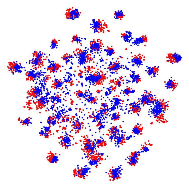
(a) DANN

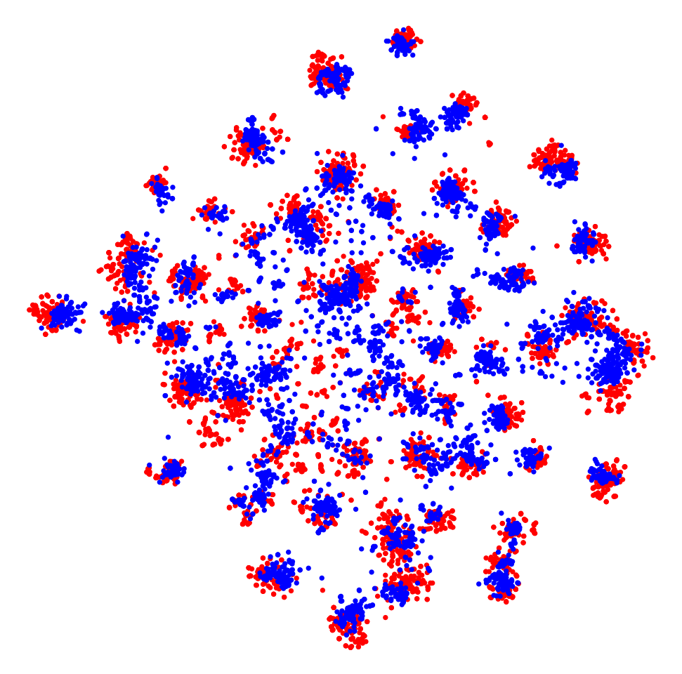
(b) BSP

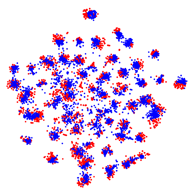
(c) NPL

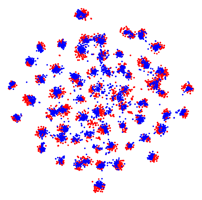
(d) SPA

Figure 2: Feature Visualization. the t-SNE plot of DANN [18], BSP [10], NPL [39], and SPA features on OfficeHome dataset in the C $\rightarrow$ R setting. We use red markers for source domain features and blue markers for target domain features.

Feature Visualization. To demonstrate the learning ability of SPA, we visualize the features of DANN [18], BSP [10], NPL [39] and SPA with the t-SNE embedding [17] under the C $\rightarrow$ R setting of OfficeHome Dataset. BSP is a classic domain adaptation method which also use matrix decomposition and NPL is a classic pseudo-labeling method which also use high-confidence predictions on unlabeled data as true labels. Thus, we choose them as baselines to compare. The results are shown in Figure 2. Comparing Figure 2(d) with Figure 2(a), Figure 2(b) and Figure 2(c) respectively, we make some important observations: (i)-we find that the clusters of features in Figure 2(d) are more compact, or say less diffuse than others, which suggests that the features learned by SPA are able to attain more desirable discriminative property; (ii)-we observe that red markers are more closer and overlapping with blue markers in Figure 2(d), which suggests that the source features and target features learned by SPA are transferred better. These observations imply the superiority of SPA over discriminability and transferability in unsupervised domain adaptation scenario.

5 Related Work

Domain Adaptation. Domain adaptation (DA) problem is a specific subject of transfer learning [90, 29], and also a widely studied area in computer vision field [18, 20, 19, 73, 52, 65, 66, 40, 44, 70, 51], By the label amount of target domain, domain adaptation can be divided into unsupervised domain adaptation, and semi-supervised domain adaptation etc. Unsupervised domain adaptation methods are very effective at aligning feature distributions of source and target domains without any target supervision but perform poorly when even a few labeled examples are available in the target. Our approach mainly focus on unsupervised domain adaptation, achieving the cutting-edge performance. It can also be extended to semi-supervised domain adaptation with comparable results.

There are more specifics of our baselines. Inspired by random walk [77] in graph theory, MCC [31] proposes a self-training method by optimizing the class confusion matrix. BNM [13] formulates the loss of nuclear norm, i.e, the sum of singular values based on the prediction outputs. NWD [8] calculates the difference between the nuclear norm of source prediction matrix and target prediction matrix. The aforementioned three methods all focus on the prediction outputs and establish class-to-class relations. Besides, there are two works focusing on the features, CORAL [70], measuring the difference of covariance, and BSP [10], directly performing singular value decomposition on features and calculate top $k$ singular values. BNM, NWD and BSP are similar to our method with the use of singular values. However, our eigenvalues comes out from the graph laplacians, which contains graph topology information [12]. For example, the second-smallest non-zero laplacian eigenvalue is called as the algebraic connectivity, and its magnitude just reflects how connected graph is [12]. As we know, we are the first to propose a graph spectral alignment perspective for domain adaptation scenarios.

Self-training. Self-training is a semi-supervised learning method that enhances supervised models by generating pseudo-labels for unlabeled data based on model predictions, which has been explored in lots of works [27, 39, 50, 83, 84, 68]. These methods pick up the class with the maximum predicted probability as true labels each time the weights are updated. With filtering strategies and iterative approaches employed to improve the quality of pseudo labels, this self-training technique has also been applied to some domain adaptation methods [48, 88, 81, 37]. This kind of methods proves beneficial when the labeled data is limited. However, it relies on an assumption of the unlabeled data following the same distribution with the labeled data and requires accurate initial model predictions for precise results [59, 2]. The intra-domain alignment in our approach helps the neighbor-aware self-training mechanism generate more precise labels. The interaction between components of our approach brings our impressive results in DA scenarios.

Graph Data Mining. Graphs are widely applied in real-world applications to model pairwise interactions between objects in numerous domains such as biology [78], social media [60] and finance [86]. Because of their rich value, graph data mining has long been an important research direction [7, 16, 36, 75]. It also plays a significant role in computer vision tasks such as image retrieval [34], object detection [46], and image classification [74]. Bruna et al.[7] first introduce the graph convolution operation based on spectral graph theory. The graph filter and the eigen-decomposition of the graph Laplacian matrix inspire us to propose our graph spectral alignment.

6 Conclusion

In this paper, we present a novel spectral alignment perspective for balancing inter-domain transferability and intra-domain discriminability in UDA. We first leveraged graph structure to model the topological information of domain graphs. Next, we aligned domain graphs in their eigenspaces and propagated neighborhood information to generate pseudo-labels. The comprehensive model analysis demonstrates the superiority of our method. The current method for constructing graph spectra is only a starting point and may be inadequate for more difficult scenarios such as universal domain adaptation. Additionally, this method is currently limited to visual classification tasks , and more sophisticated and generic methods to object detection or semantic segmentation are expected in the future. Furthermore, we believe that graph data mining methods and the well-formulated properties of graph spectra should have more discussion in both domain adaptation and computer vision field.

7 Acknowledgement

This work is majorly supported in part by the National Key Research and Development Program of China (No. 2022YFB3304100), the NSFC under Grants (No. 62206247), and by the Fundamental Research Funds for the Central Universities (No. 226-2022-00028). JZ also thanks the sponsorship by CAAI-Huawei Open Fund.

Appendix A More Setups

Hardware and Software Configurations. All experiments are conducted on a server with the following configurations:

• Operating System: Ubuntu 20.04.4 LTS

• CPU: Intel(R) Xeon(R) Platinum 8358P CPU @ 2.60GHz, 32 cores, 128 processors

• GPU: NVIDIA GeForce RTX 3090

More Implementation Details. We use PyTorch and tllib toolbox [28] to implement our method and fine-tune ResNet pre-trained on ImageNet [25, 26]. Following the standard protocols for unsupervised domain adaptation in previous methods [48, 56], we use the same backbone networks for fair comparisons. For Office31 and OfficeHome dataset, we use ResNet-50 as the backbone network. For VisDA2017 and DomainNet dataset, we use ResNet-101 as the backbone network. Following previous work [48], we adopt mini-batch stochastic gradient descent (SGD) to learn the feature encoder by fine-tuning from the ImageNet pre-trained model with the learning rate 0.001, and new layers, as bottleneck layer and classification layer. The learning rates of the layers trained from scratch are set to be 0.01. We use the the same learning rate schedule in [48, 52], including a learning rate scheduler with a momentum of 0.9, a weight decay of 0.005, the bottleneck size of 256, and batch size of 32.

We report main experimental results with the average accuracy over 5 random trials with the initial seed 0. For transductive unsupervised domain adaptation, the reported accuracy is computed on the complete unlabeled target data, following established protocol for UDA [18, 52, 31, 10, 48]. For inductive unsupervised domain adaptation on DomainNet, the reported accuracy is computed on the provided test dataset.. We use a standard batch size of 32 for both source and target in all experiments and for all variants of our method. The reverse validation [47, 89] is conducted to select hyper-parameters. For both unsupervised domain adaptation (UDA) and semi-supervised domain adaptation (SSDA) scenarios, we fix the coefficient of $\mathcal{L}_{nap}$ as 0.2 and the coefficient of $\mathcal{L}_{gsa}$ as 1.0, while we will offer a sensitivity analysis for this two coefficients in the following section. More details refer to our code in the supplemental materials.

Appendix B More Experiments

B.1 Unsupervised Domain Adaptation

In the main paper, we present the classification accuracy results on VisDA2017 dataset for unsupervised domain adaptation and leave out per-category accuracy details. In the appendix, Table 5, we give the full table on VisDA2017, using ResNet101 as backbone. Looking into this table, we can find that our SPA model consistently outperforms most of domain adaptation methods. For classic baselines, we improve DANN [18] by 30.3%, and CDAN [52] by 14 %. For recent and state-of-the-art baselines, our results is 4% higher than NWD [8] and 0.5 % better than FixBi [56]. Our SPA model ranks top in 6 out of 12 categories, ranks top 2 in 9 out of 12 categories, and SPA also achieves the best classification accuracy in total.

Furthermore, in the main paper, we present the classification accuracy results on original DomainNet with 365 categories. While the original DomainNet dataset has noisy labels, the previous work [64] use a subset of it that contains 126 categories from C, P, R and S, 4 domains in total, which we refer to as DomainNet126. In the appendix, Table 6, we show the results on DomainNet126. Our SPA model consistently ranks top among 12 tasks across 4 domains and achieves the best accuracy of 77.1 %, which is 12.3 % better than the second one. For classic baselines, we improve DANN [18] by 20.2 %, and CDAN [52] by 16 %.

Table 5: Per-category Accuracy (%) on VisDA2017 for unsupervised domain adaptation, using ResNet101 as backbone. All the results are based on ResNet101 except those with mark ^†, which are based on ResNet50. The best accuracy is indicated in bold and the second best one is underlined.

Method	aero	bike	bus	car	horse	knife	motor	person	plant	skate	train	truck	Avg.
Source Only [25]	55.1	53.3	61.9	59.1	80.6	17.9	79.7	31.2	81.0	26.5	73.5	8.5	52.4
DANN [18]	81.9	77.7	82.8	44.3	81.2	29.5	65.1	28.6	51.9	54.6	82.8	7.8	57.4
CDAN [52]	85.2	66.9	83.0	50.8	84.2	74.9	88.1	74.5	83.4	76.0	81.9	38.0	73.7
MixMatch [5]	93.9	71.8	93.5	82.1	95.3	0.7	90.8	38.1	94.5	96.0	86.3	2.2	70.4
BSP [10]	92.4	61.0	81.0	57.5	89.0	80.6	90.1	77.0	84.2	77.9	82.1	38.4	75.9
NPL [39]	90.9	74.6	73.2	55.8	89.6	64.6	86.8	68.7	90.7	64.8	89.5	47.7	74.7
GVB [14]	-	-	-	-	-	-	-	-	-	-	-	-	75.3†
MCC [31]	92.2	82.9	76.8	66.6	90.9	78.5	87.9	73.8	90.1	76.1	87.1	41.0	78.8
BNM [13]	93.6	68.3	78.9	70.3	91.1	82.8	93.0	78.7	90.9	76.5	89.1	40.9	79.5
ATDOC [48]	95.3	84.7	82.4	75.6	95.8	97.7	88.7	76.6	94.0	91.7	91.5	61.9	86.3
FixBi [56]	96.1	87.8	90.5	90.3	96.8	95.3	92.8	88.7	97.2	94.2	90.9	25.7	87.2
SDAT [62]	94.8	77.1	82.8	60.9	92.3	95.2	91.7	79.9	89.9	91.2	88.5	41.2	82.1
NWD [8]	96.1	82.7	76.8	71.4	92.5	96.8	88.2	81.3	92.2	88.7	84.1	53.7	83.7
SPA (Ours)	98.5	92.2	86.3	63.0	97.5	95.4	93.5	80.7	97.2	95.2	91.1	61.4	87.7

Table 6: Classification Accuracy (%) on DomainNet126 for unsupervised domain adaptation, using ResNet101 as backbone. The best accuracy is indicated in bold and the second best one is underlined.

Method	C$\rightarrow$P	C$\rightarrow$R	C$\rightarrow$S	P$\rightarrow$C	P$\rightarrow$R	P$\rightarrow$S	R$\rightarrow$C	R$\rightarrow$P	R$\rightarrow$S	S$\rightarrow$C	S$\rightarrow$P	S$\rightarrow$R	Avg.
Source Only [25]	38.4	50.9	43.9	50.3	66.7	39.9	54.6	57.9	43.7	52.5	43.5	48.3	49.2
DANN [18]	46.5	58.2	51.6	52.7	64.2	52.9	61.7	60.3	53.9	62.7	56.7	61.6	56.9
MCD [66]	43.7	55.7	47.6	51.9	67.8	45.0	52.9	57.3	40.4	56.3	50.8	56.8	52.3
BSP [10]	45.7	58.7	55.5	48.6	65.2	48.6	55.2	60.8	48.6	56.8	55.8	61.4	55.1
CDAN [52]	50.9	61.6	54.8	59.4	68.5	55.5	70.4	66.9	57.7	64.2	59.1	64.3	61.1
SAFN [85]	50.0	58.7	52.4	56.3	73.7	53.5	55.8	64.8	48.5	60.7	59.5	64.3	58.2
RSDA [23]	45.5	56.6	46.6	45.7	60.4	48.6	54.6	61.5	50.9	56.1	54.0	58.6	53.4
PAN [79]	58.8	65.2	54.6	57.5	70.5	53.1	67.6	66.7	55.9	64.4	60.2	66.6	61.8
MemSAC [33]	53.6	66.5	58.8	63.2	71.2	58.1	73.2	70.5	61.5	68.8	64.1	67.6	64.8
SPA (Ours)	73.5	84.0	70.6	76.5	85.9	71.9	76.6	77.0	69.8	78.3	76.8	83.9	77.1

Table 7: Classification Accuracy (%) on DomainNet126 for 1-shot and 3-shot semi-supervised domain adaptation, using ResNet34 as backbone. The best accuracy is indicated in bold and the second best one is underlined.

Method	C$\rightarrow$S		P$\rightarrow$C		P$\rightarrow$R		R$\rightarrow$C		R$\rightarrow$P		R$\rightarrow$S		S$\rightarrow$P		Avg.
	1-	3-	1-	3-	1-	3-	1-	3-	1-	3-	1-	3-	1-	3-	1-	3-
S + T [25]	54.8	57.9	59.2	63.0	73.7	75.6	61.2	63.9	64.5	66.3	52.0	56.0	60.4	62.2	60.8	63.6
DANN [18]	52.8	55.4	70.3	72.2	56.3	59.6	58.2	59.8	61.4	62.8	52.2	54.9	57.4	59.9	58.4	60.7
ENT [21]	54.6	60.0	65.4	71.1	75.0	78.6	65.2	71.0	65.9	69.2	52.1	61.1	59.7	62.1	62.6	67.6
MME [64]	56.3	61.8	69.0	71.7	76.1	78.5	70.0	72.2	67.7	69.7	61.0	61.9	64.8	66.8	66.4	68.9
APE [35]	56.7	63.1	72.9	76.7	76.6	79.4	70.4	76.6	70.8	72.1	63.0	67.8	64.5	66.1	67.6	71.7
BiAT [30]	57.9	61.5	71.6	74.6	77.0	78.6	73.0	74.9	68.0	68.8	58.5	62.1	63.9	67.5	67.1	69.7
MixMatch [5]	59.3	62.7	66.7	68.7	74.8	78.8	69.4	72.6	67.8	68.8	62.5	65.6	66.3	67.1	66.7	69.2
NPL [39]	62.5	64.5	67.6	70.7	78.3	79.3	70.9	72.9	69.2	70.7	62.0	64.8	67.0	68.6	68.2	70.2
BNM [13]	58.4	62.6	69.4	72.7	77.0	79.5	69.8	73.7	69.8	71.2	61.4	65.1	64.1	67.6	67.1	70.3
MCC [31]	56.8	60.5	62.8	66.5	75.3	76.5	65.5	67.2	66.9	68.1	57.6	59.8	63.4	65.0	64.0	66.2
ATDOC [48]	65.6	66.7	72.8	74.2	81.2	81.2	74.9	76.9	71.3	72.5	65.2	64.6	68.7	70.8	71.4	72.4
AESL [61]	59.5	65.2	74.6	76.2	72.4	74.1	74.8	77.3	79.4	80.5	66.2	69.5	66.6	69.6	70.5	73.2
SPA (Ours)	65.9	67.0	74.8	76.5	81.1	82.3	75.3	76.0	71.8	72.2	65.8	67.2	69.8	71.1	72.1	73.2

Table 8: Classification Accuracy (%) on OfficeHome for 1-shot and 3-shot semi-supervised domain adaptation, using ResNet34 as backbone. The best accuracy is indicated in bold and the second best one is underlined.

Method (1-shot)	A$\rightarrow$C	A$\rightarrow$P	A$\rightarrow$R	C$\rightarrow$A	C$\rightarrow$P	C$\rightarrow$R	P$\rightarrow$A	P$\rightarrow$C	P$\rightarrow$R	R$\rightarrow$A	R$\rightarrow$C	R$\rightarrow$P	Avg.
S + T [25]	52.1	78.6	66.2	74.4	48.3	57.2	69.8	50.9	73.8	70.0	56.3	68.1	63.8
DANN [18]	53.1	74.8	64.5	68.4	51.9	55.7	67.9	52.3	73.9	69.2	54.1	66.8	62.7
ENT [21]	53.6	81.9	70.4	79.9	51.9	63.0	75.0	52.9	76.7	73.2	63.2	73.6	67.9
MME [64]	61.9	82.8	71.2	79.2	57.4	64.7	75.5	59.6	77.8	74.8	65.7	74.5	70.4
APE [35]	60.7	81.6	72.5	78.6	58.3	63.6	76.1	53.9	75.2	72.3	63.6	69.8	68.9
CDAC [41]	61.9	83.1	72.7	80.0	59.3	64.6	75.9	61.2	78.5	75.3	64.5	75.1	71.0
SPA (Ours)	62.3	76.7	79.0	66.6	77.3	76.4	65.7	59.1	80.7	71.4	65.2	84.1	72.0
Method (3-shot)	A$\rightarrow$C	A$\rightarrow$P	A$\rightarrow$R	C$\rightarrow$A	C$\rightarrow$P	C$\rightarrow$R	P$\rightarrow$A	P$\rightarrow$C	P$\rightarrow$R	R$\rightarrow$A	R$\rightarrow$C	R$\rightarrow$P	Avg.
S + T [25]	55.7	80.8	67.8	73.1	53.8	63.5	73.1	54.0	74.2	68.3	57.6	72.3	66.2
DANN [18]	57.3	75.5	65.2	69.2	51.8	56.6	68.3	54.7	73.8	67.1	55.1	67.5	63.5
ENT [21]	62.6	85.7	70.2	79.9	60.5	63.9	79.5	61.3	79.1	76.4	64.7	79.1	71.9
MME [64]	64.6	85.5	71.3	80.1	64.6	65.5	79.0	63.6	79.7	76.6	67.2	79.3	73.1
APE [35]	66.4	86.2	73.4	82.0	65.2	66.1	81.1	63.9	80.2	76.8	66.6	79.9	74.0
CDAC [41]	67.8	85.6	72.2	81.9	67.0	67.5	80.3	65.9	80.6	80.2	67.4	81.4	74.2
SPA (Ours)	63.1	81.0	80.2	68.5	81.7	77.5	69.5	65.2	82.0	73.9	67.2	87.0	74.7

B.2 Semi-supervised Domain Adaptation

We also extend our SPA model to semi-superivsed domain adaptation (SSDA) scenario and conduct experiments on 1-shot and 3-shot setting, and S + T in SSDA task means the model trained only by the labeled source and target data.

We present the classificaition accuracy results on DomainNet126 and OfficeHome datasets for SSDA scenario in the Table 7 and Table 8 respectively. Looking at the details, Table 7 shows the classification results for 1-shot and 3-shot SSDA setting on DomainNet126 dataset. For the 1-shot setting, our SPA model can improve DANN [18] by 13.7 % and ENT [21] by 9.5 %. our SPA consistently ranks top among 4 out of 7 tasks and ranks top 2 among all tasks, achieving the best accuracy of 72.1 %, which is better 1.6 % then the second one. For the 3-shot setting, our SPA model can improve DANN [18] by 12.5 % and ENT [21] by 5.6 %. SPA achieves the best accuracy of 73.2 %, comparable with recent work AESL [61].

Furthermore, Table 8 shows the classification results for 1-shot and 3-shot SSDA setting on OfficeHome dataset. To verify that our SPA model can also generalize to SSDA scenario, we compare SPA with several classic and recent baselines. The first section of the table shows our SPA model can improve DANN [18] by 9.3 % and ENT [21] by 4.1 % in the 1-shot setting. The second section shows our SPA model can improve DANN [18] by 11.2 % and ENT [21] by 2.8 % in the 3-shot setting. This shows that our SPA model can greatly improve the classic baselines and achieve comparable results with CDAC [41].

B.3 Model Analysis

Robustness Analysis. In the main paper, we have already verified the robustness of SPA to different graph structures on OfficeHome dataset. In the appendix, we further show the experimental results on Office31 dataset in Table 9. Similarly, we conduct experiments on different types of Laplacian matrix, similarity metric of graph relations, and $k$ number of nearest neighbors of KNN classification methods. The Laplacian matrices are chosen from the random walk laplacian matrix $\mathbf{L}_{rwk}=\mathbf{D}^{-1}\mathbf{A}$, and the symmetrically normalized Laplacian matrix $\mathbf{L}_{sym}=\mathbf{I}-\mathbf{D}^{-1/2}\mathbf{A}\mathbf{D}^{-1/2}$, where $\mathbf{D}$ denotes the degree matrix based on the adjacency matrix $\mathbf{A}$. In addition, the similarity metrics are chosen from cosine similarity and Gaussian similarity, and different $k=3,5$ when applying KNN classification algorithm. From Table 9, We can find that different types of Laplacian matrix still lead to comparable results. As for the similarity metric, the Gaussian similarity brings better performance than cosine similarity. On Office31 dataset, 5-NN graphs is superior than 3-NN graphs when combining with $\mathbf{L}_{rwk}$, and comparable when combining with $\mathbf{L}_{sym}$. For all these aforementioned experiments results, the differences between them are within 1% around, confirming the robustness of SPA.

Table 9: Classification Accuracy (%) on OfficeHome for unsupervised domain adaptation. The table is divided into three sections corresponding to robustness analysis, and parameter sensitivity, each separated by a double horizontal line.

Method	A$\rightarrow$D	A$\rightarrow$W	D$\rightarrow$A	D$\rightarrow$W	W$\rightarrow$A	W$\rightarrow$D	Avg.
$\beta$ = 0.1	94.2	95.1	76.6	98.9	78.6	99.6	90.5
$\beta$ = 0.3	94.0	96.2	76.9	98.9	79.3	99.8	90.8
$\beta$ = 0.5	94.0	96.4	77.9	99.0	78.0	99.8	90.8
$\beta$ = 0.7	94.4	96.0	79.0	98.6	80.3	100.	91.4
$\beta$ = 0.8	94.2	95.7	76.1	98.6	78.3	99.8	90.5
$\mathbf{L}_{rwk}$ w/ $cos$	93.8	95.0	76.3	98.6	79.7	100.	90.6
$\mathbf{L}_{rwk}$ w/ $gauss$	95.0	95.6	78.2	98.6	80.0	99.8	91.2
$\mathbf{L}_{sym}$ w/ $cos$	93.8	93.8	78.5	98.6	79.9	100.	90.8
$\mathbf{L}_{sym}$ w/ $gauss$	93.8	95.6	79.4	98.6	78.8	99.8	91.0
$\mathbf{L}_{rwk}$ w/ $k$ = 3	93.8	95.2	78.3	98.9	80.4	99.8	91.1
$\mathbf{L}_{rwk}$ w/ $k$ = 5	93.8	95.0	76.3	98.6	79.7	100.	90.6
$\mathbf{L}_{sym}$ w/ $k$ = 3	94.0	95.8	75.2	99.0	80.5	100.	90.7
$\mathbf{L}_{sym}$ w/ $k$ = 5	93.8	93.8	78.5	98.6	79.9	100.	90.8

Parameter Sensitivity. In the main paper, we have already analyzed the experiments on the hyperparameter $\beta$ of exponential moving averaging strategy for memory updates and verify that SPA is insensitive to this hyperparameter. Here, we show the experimental results on Office31 dataset in Table 9. Similarly, we design experiments on the hyperparameter $\beta$ of exponential moving averaging strategy for memory updates, choosing $\beta$ = 0.1, 0.3, 0.5, 0.7, 0.9 respectively. These results are based on DANN [18]. From the series of results, we can find that in Office31 dataset, the choice of $\beta$ = 0.7 outperforms than others. In addition, the differences between these results are within 1.0%, which means that SPA is relatively stable to this hyperparameter.

Furthermore, we design experiments for the coefficient of $\mathcal{L}_{nap}$ and the coefficient of $\mathcal{L}_{gsa}$ to analyze the stability of SPA. The experimental results are shown in the Figure 3. These results are based on DANN [18]. Fixing the coefficient of $\mathcal{L}_{nap}$ = 0.2, the coefficient of $\mathcal{L}_{gsa}$ changes from 0.1 to 0.9. Fixing the coefficient of $\mathcal{L}_{gsa}$ = 1.0, the coefficient of $\mathcal{L}_{nap}$ changes from 0.1 to 0.9. From the series of results, we can find that in OfficeHome dataset, the choice of different coefficients result in similar results, which means that SPA is insensitive to these coefficients.

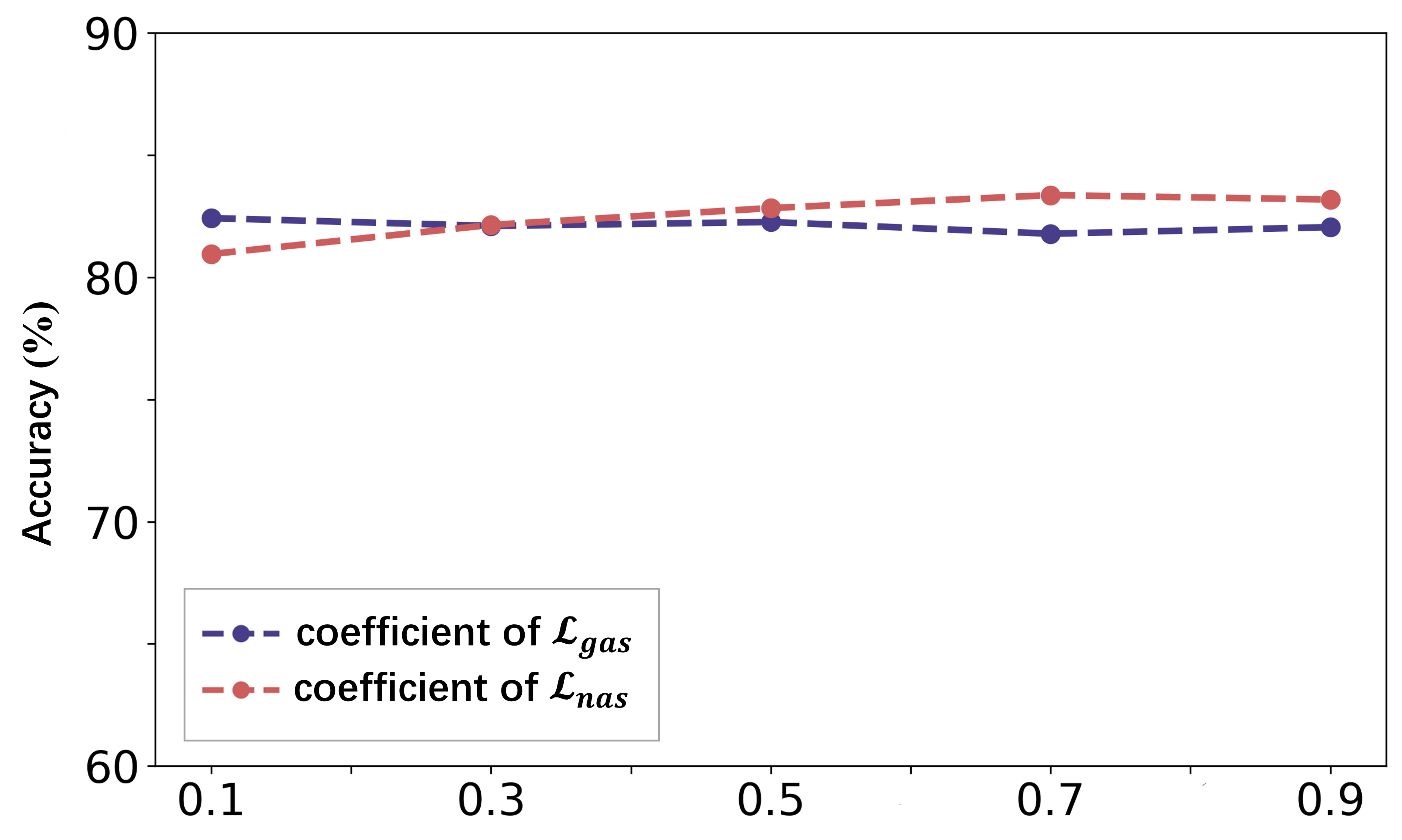
(a) A $\rightarrow$ C

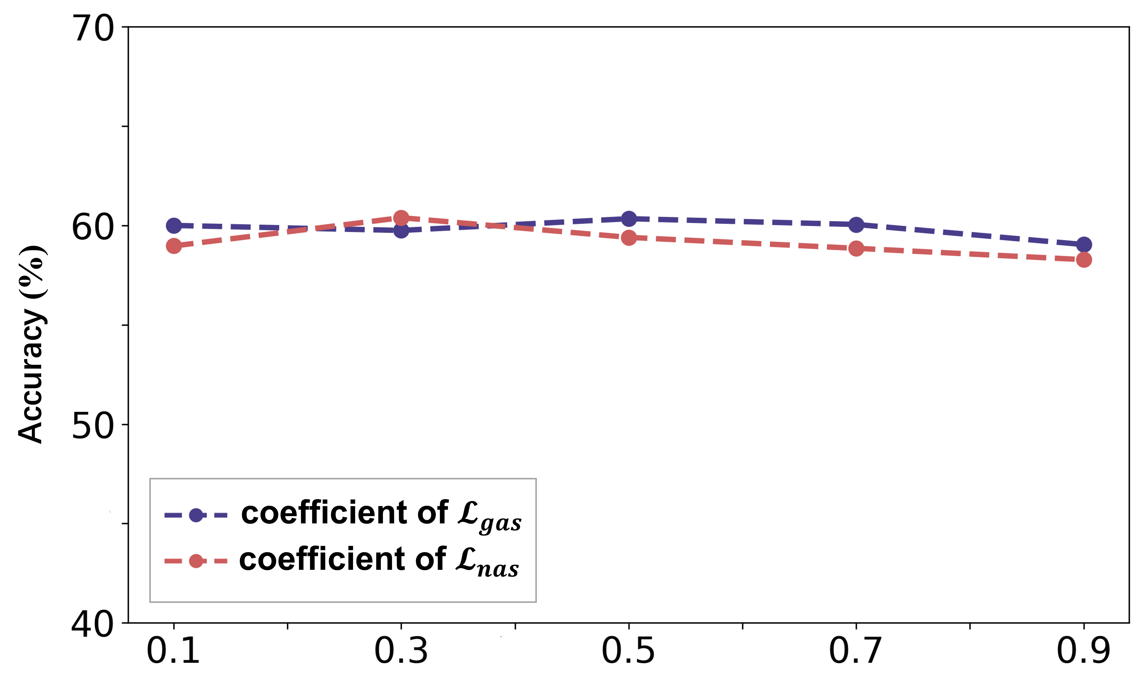
(b) C $\rightarrow$ R

Figure 3: Parameter Sensitivity. The line plot of the coefficient of $\mathcal{L}_{nap}$ and the coefficient of $\mathcal{L}_{gsa}$ change from 0.1 to 0.9, leading to different accuracy results. The experiments are conducted on OfficeHome dataset, where (a) is A $\rightarrow$ C setting and (b) is C $\rightarrow$ R setting.

Transferability and Discriminability. The $\mathcal{A}$-distance [4] measures the distribution discrepancy that is defined as $d_{\mathcal{A}}=2\left(1-2\epsilon\right)$, where $\epsilon$ is the classifier loss to discriminate the souce and target domains. Smaller $\mathcal{A}$-distance indicates better domain-invariant features. Figure 4(a) shows that SPA can achieve a lower $d_{\mathcal{A}}$, implying a lower generalization error. Furthermore, following previous work [10], we further offer the source accuracy and target accuracy specifically, in Figure 4(b) and Figure 4(c). We can find that various methods achieve similar results of source accuracy, and SPA can always achieve higher target accuracy. Combined with the experimental results in Figure 4(a), this reveals that SPA enhances transferability while still keep a strong discriminability. Back to our Introduction, this means that SPA can find a more suitable utilization of intra-domain information and inter-domain information to properly align target samples.

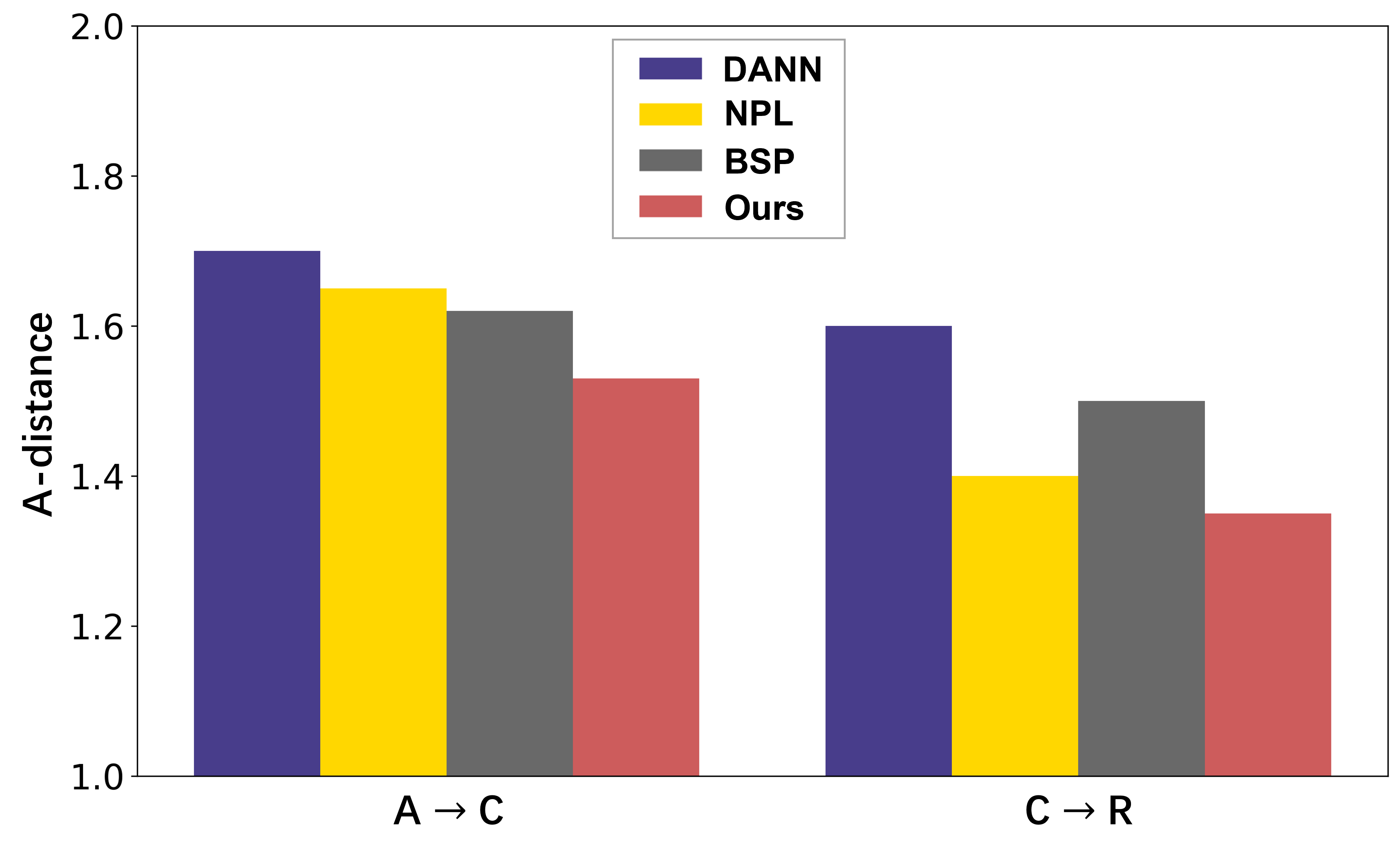
(a) A-distance

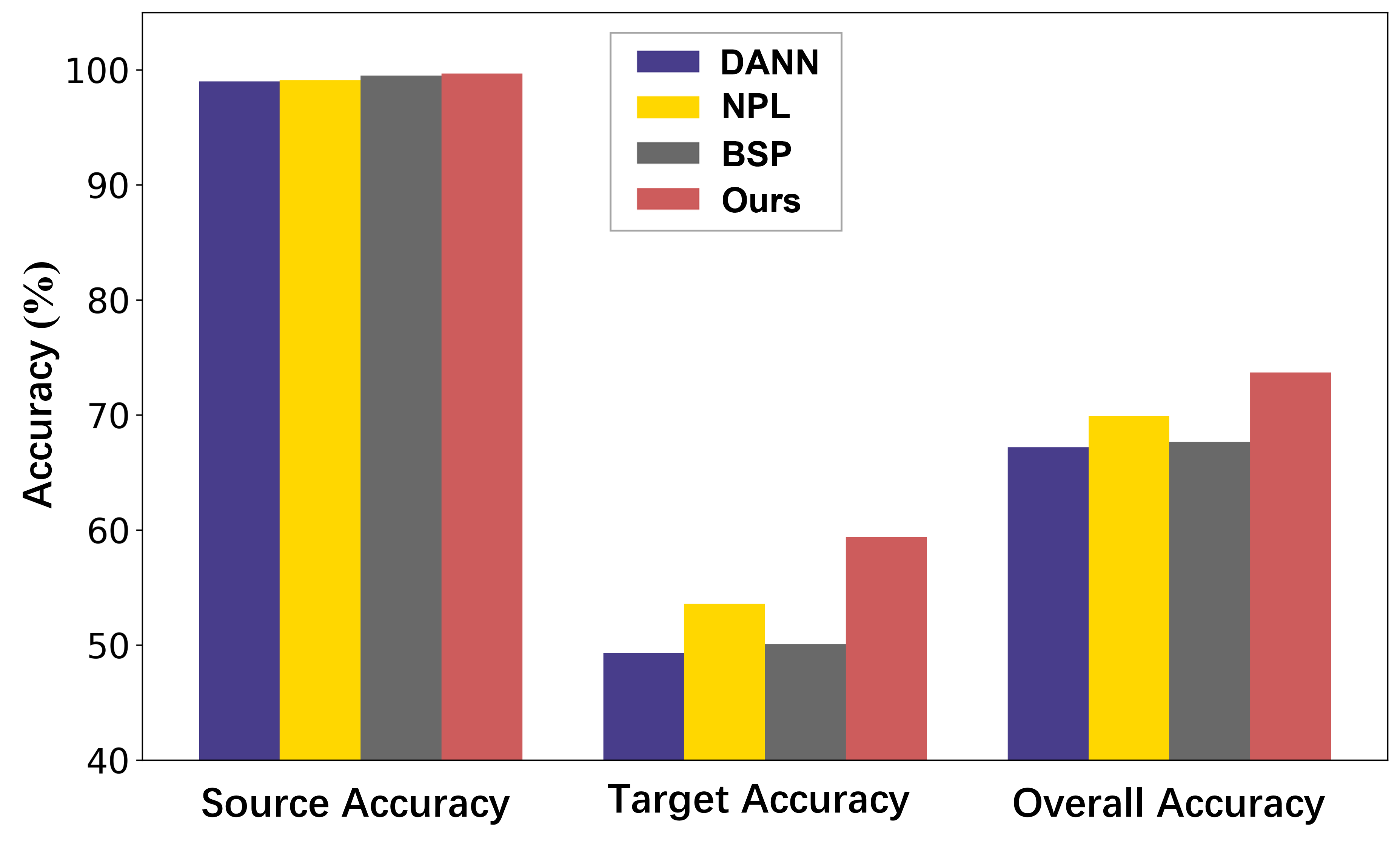
(b) A $\rightarrow$ C

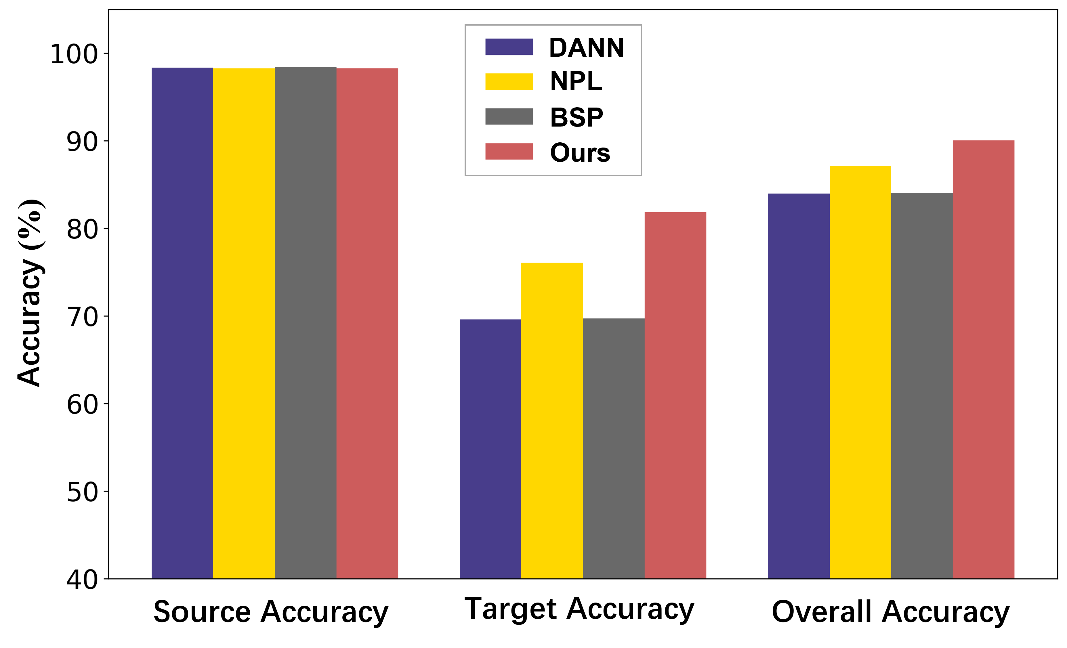
(c) C $\rightarrow$ R

Figure 4: Transferability and Discriminability. We compare SPA with DANN [18], BSP [10] and NPL [39] on OfficeHome dataset, where (a) is $\mathcal{A}$-distance in A $\rightarrow$ C and C $\rightarrow$ R setting, (b) is accuracy results in A $\rightarrow$ C setting and (c) is accuracy results in C $\rightarrow$ R setting.

Feature Visualization. To demonstrate the learning ability of SPA, we visualize the features of DANN [18], BSP [13], NPL [39] and SPA with the t-SNE embedding [17] under the C $\rightarrow$ R setting of OfficeHome Dataset in the main paper, referred as Figure 2. In the appendix, we offer more visualization figures, including Figure 5 in A $\rightarrow$ D setting and Figure 6 in A $\rightarrow$ W setting on Office31 dataset, Figure 7 in A $\rightarrow$ C setting on OfficeHome dataset. According to all the figures, the observations are consistent that the source features and target features learned by SPA are transferred better. These observations imply the superiority of SPA over discriminability and transferability in unsupervised domain adaptation scenario.

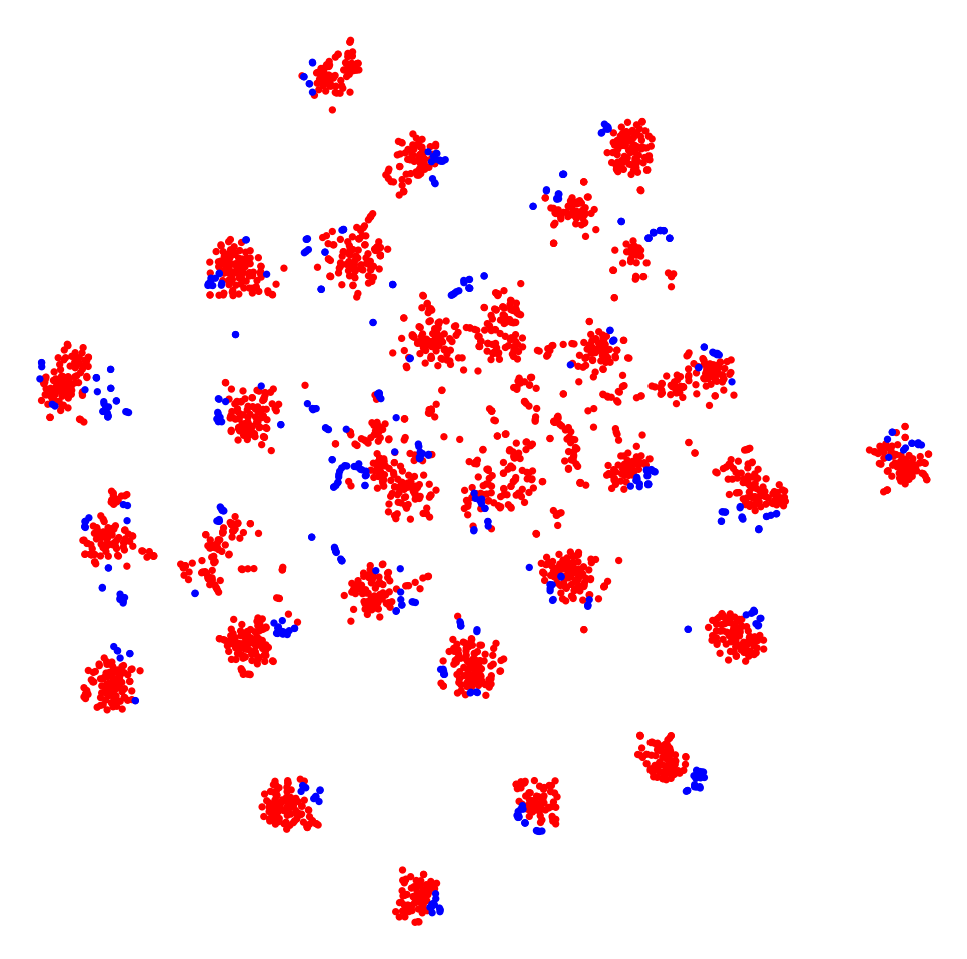
(a) DANN

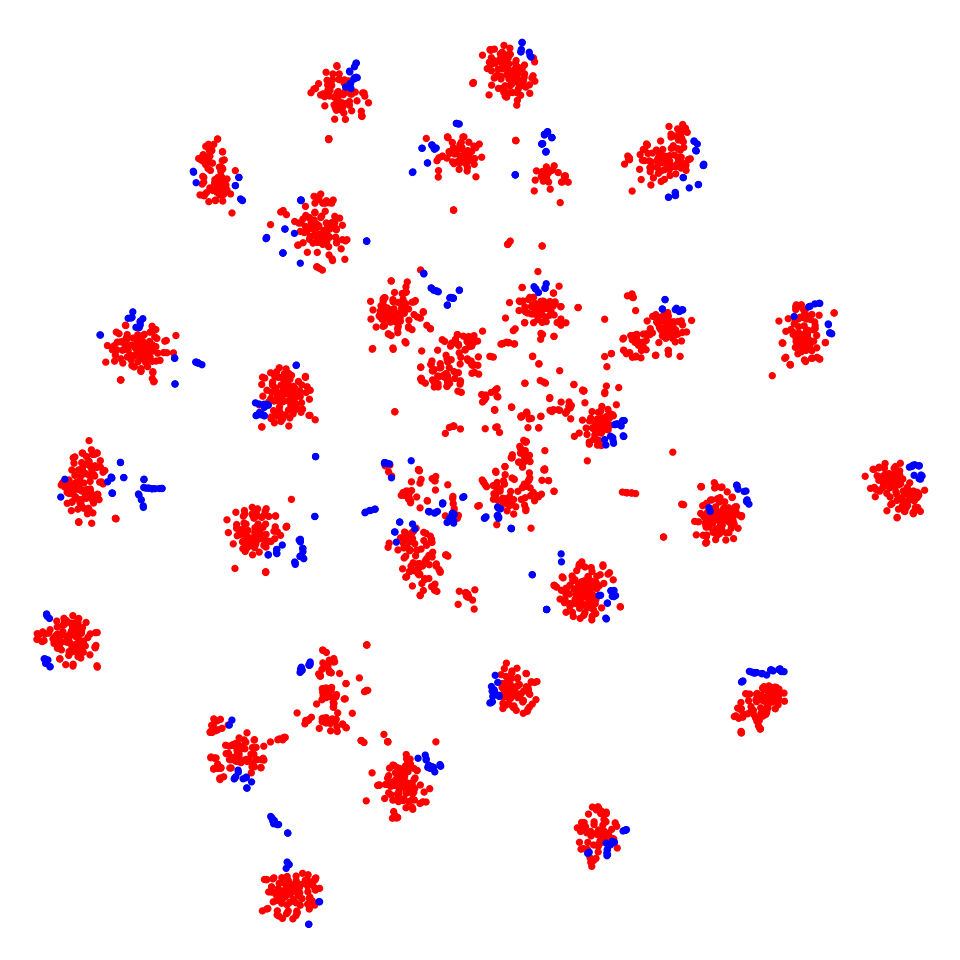
(b) BSP

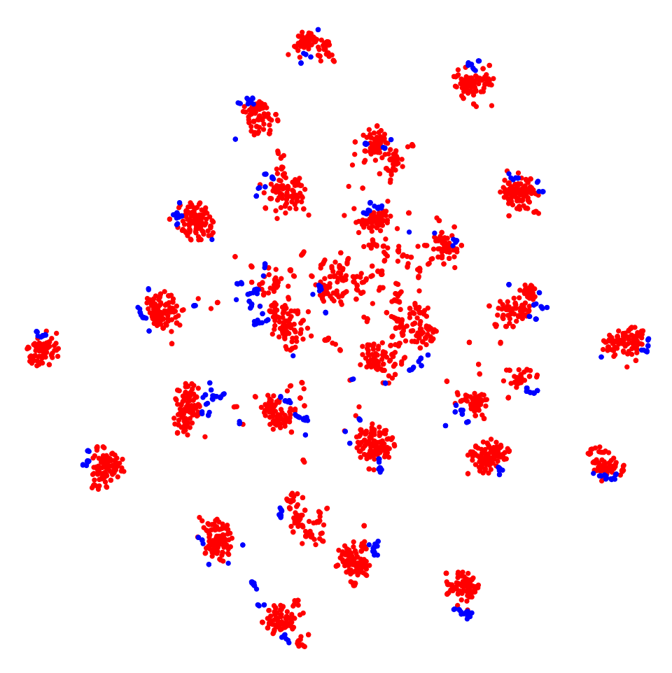
(c) NPL

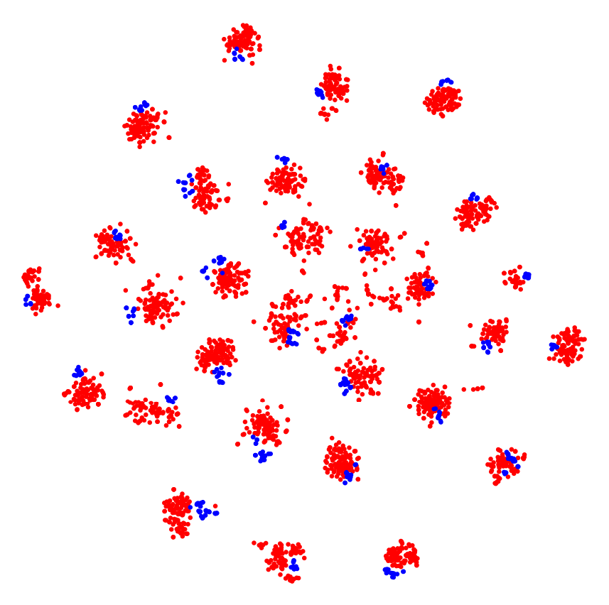
(d) SPA

Figure 5: Feature Visualization. the t-SNE plot of DANN [18], BSP [13], NPL [39], and SPA features on office31 dataset in the A $\rightarrow$ D setting. We use red markers for source domain features and blue markers for target domain features.

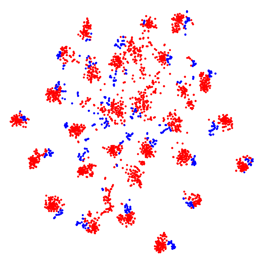
(a) DANN

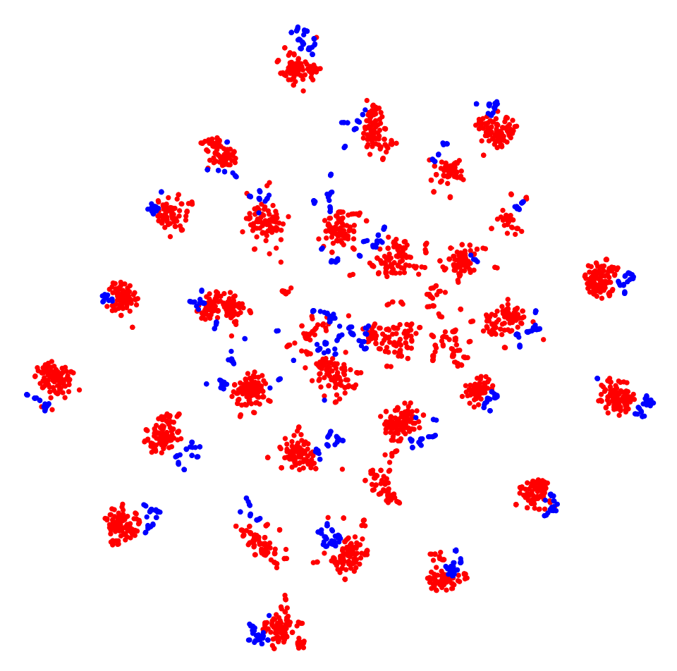
(b) BSP

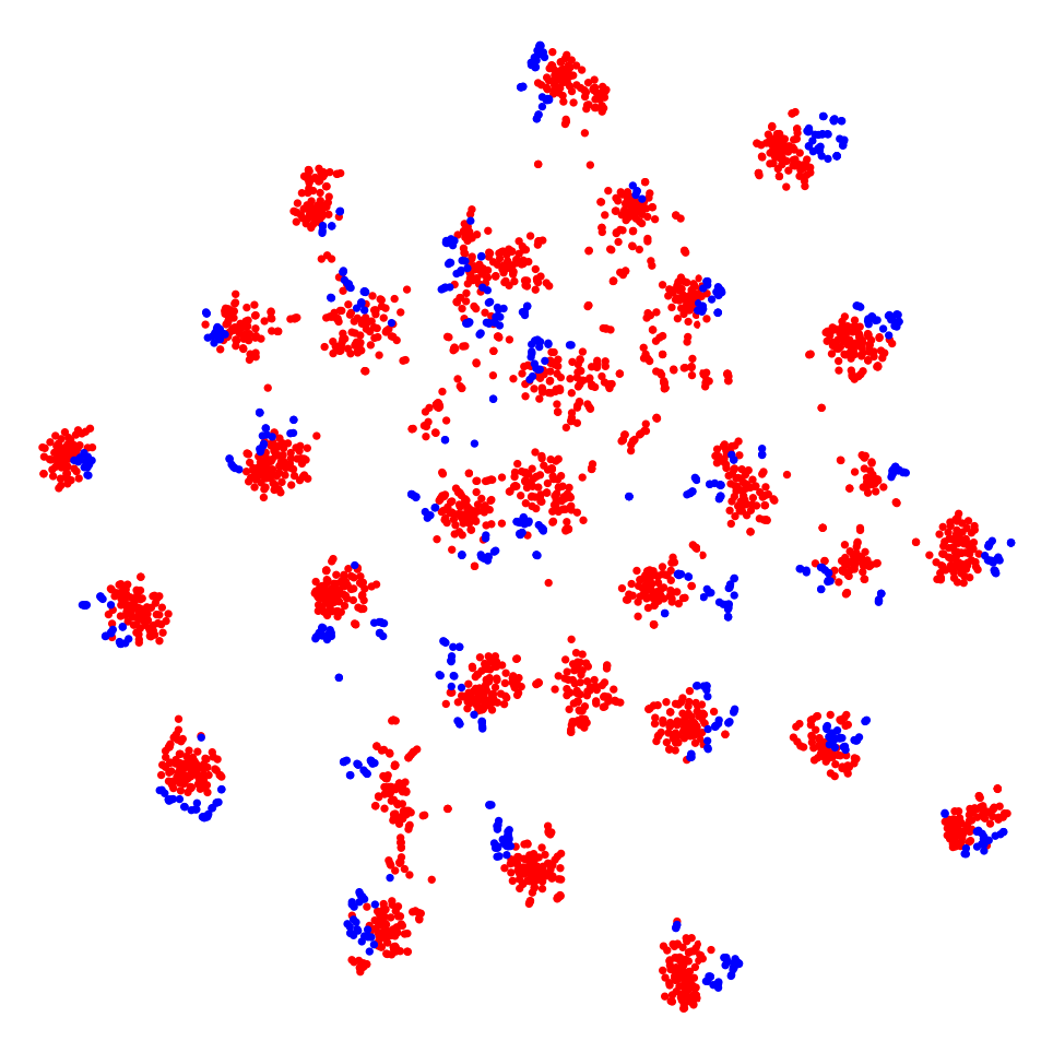
(c) NPL

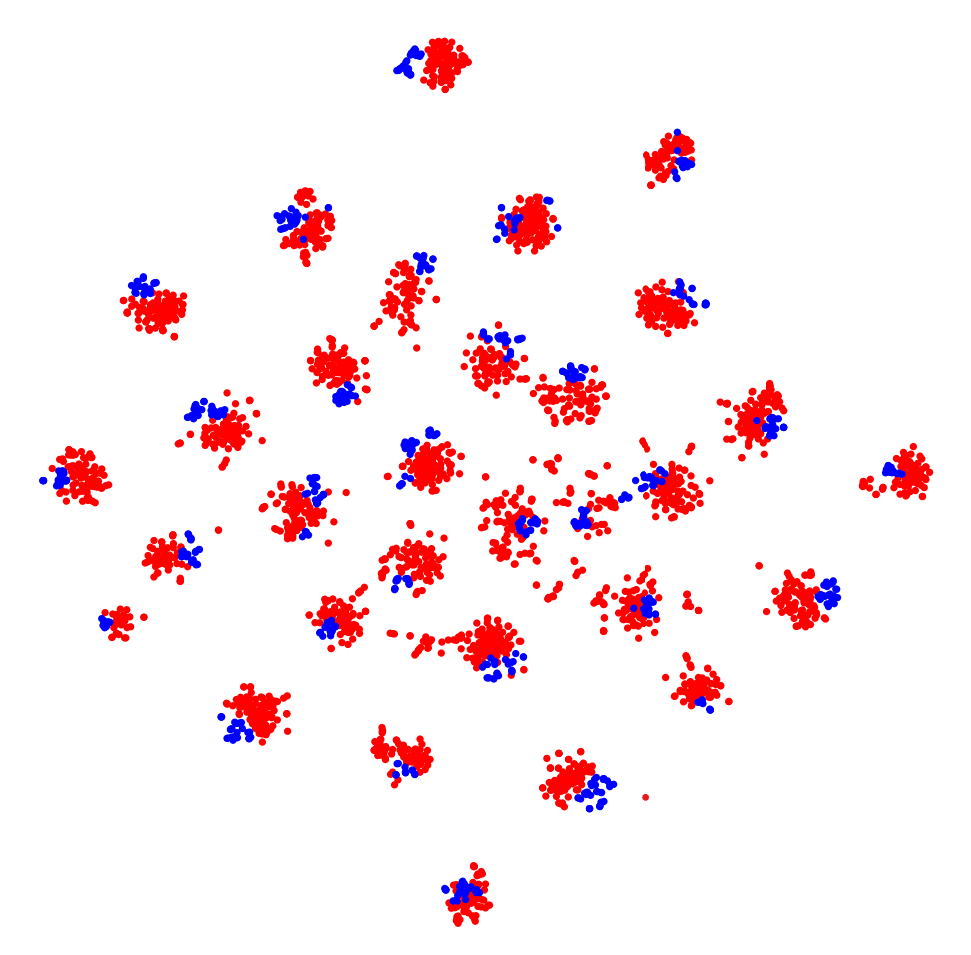
(d) SPA

Figure 6: Feature Visualization. the t-SNE plot of DANN [18], BSP [13], NPL [39], and SPA features on Office31 dataset in the A $\rightarrow$ W setting. We use red markers for source domain features and blue markers for target domain features.

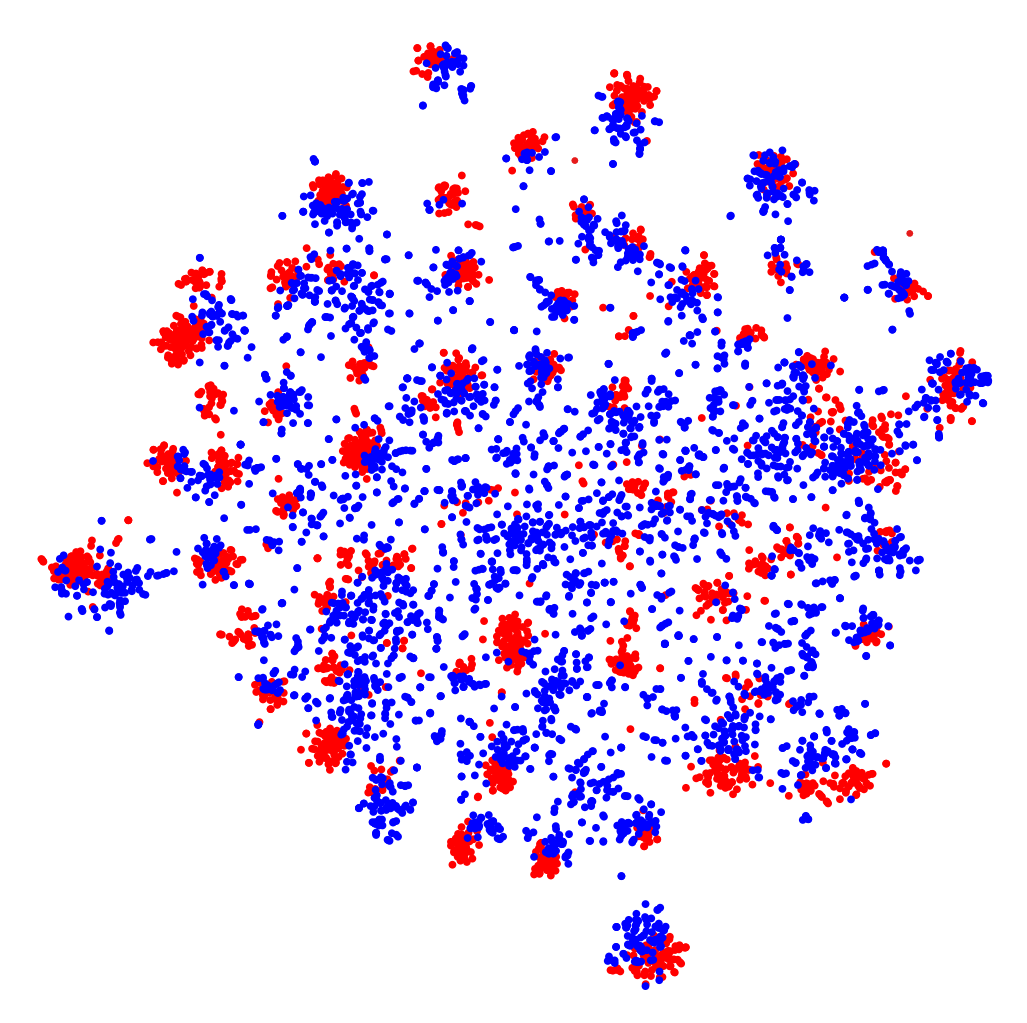
(a) DANN

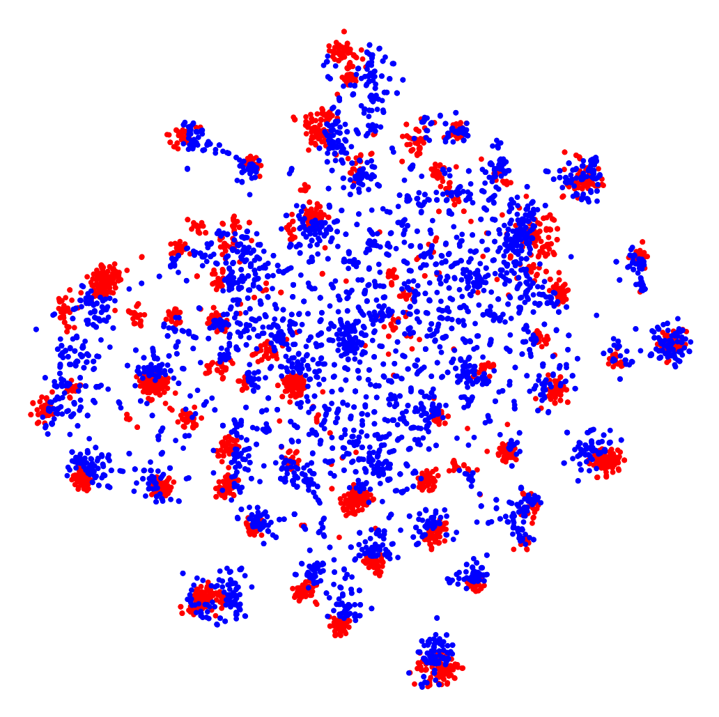
(b) BSP

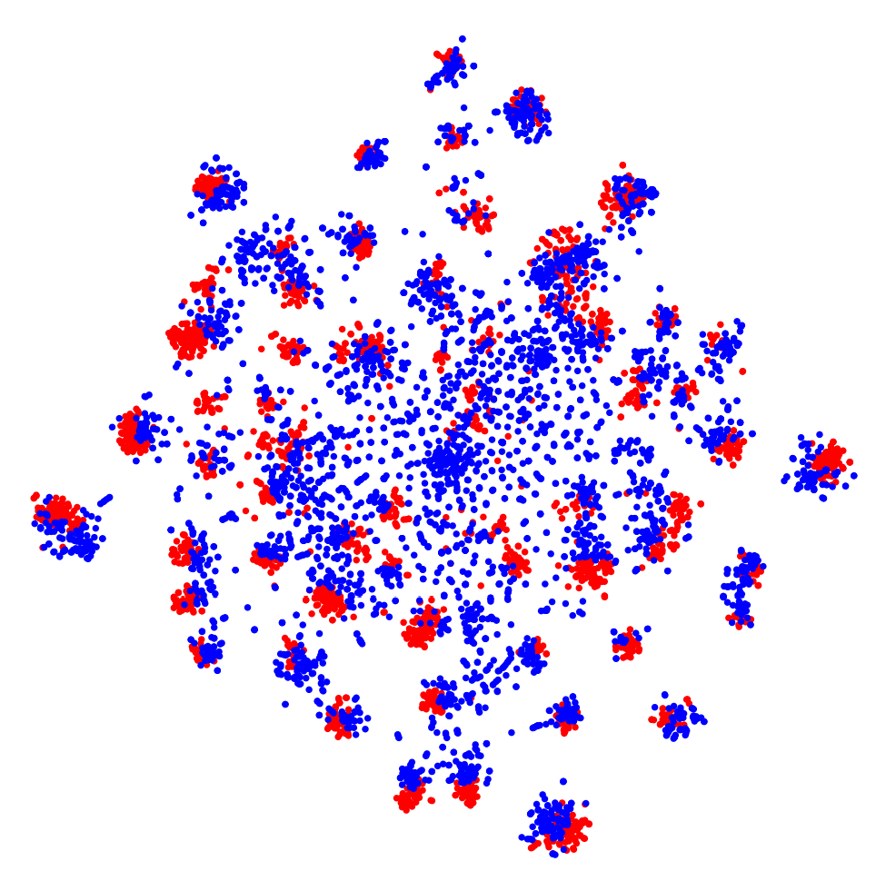
(c) NPL

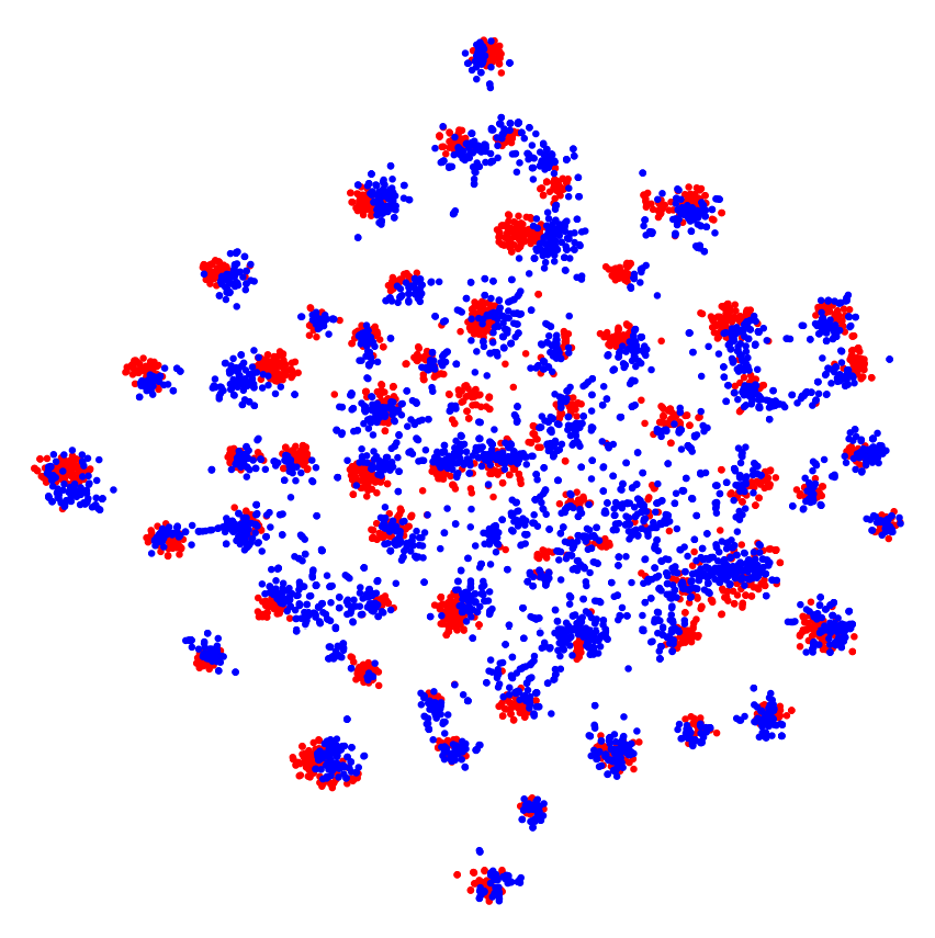
(d) SPA

Figure 7: Feature Visualization. the t-SNE plot of DANN [18], BSP [13], NPL [39], and SPA features on OfficeHome dataset in the A $\rightarrow$ C setting. We use red markers for source domain features and blue markers for target domain features.

Convergence Analysis. To demonstrate the convergence of SPA, we visualize the changes of accuracy and training loss respectively during the training process. As shown in Figure 8, the red curve is the changes of accuracy and the blue curve is the changes of training loss. The experiments are conducted on OfficeHome dataset, where 8(a) and 8(b) are in A $\rightarrow$ P setting, 8(c) and 8(d) are in R $\rightarrow$ A setting. Based on our experiments, it is evident that the model demonstrates satisfactory convergence properties. Through multiple iterations and varied initial settings, the model consistently approached and reached a stable state,

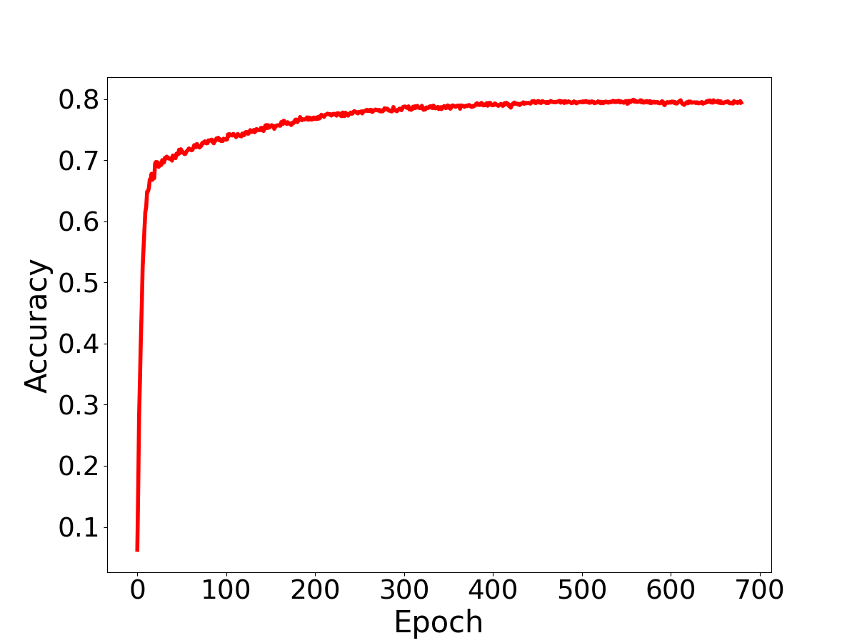
(a) The curve of accuracy under A $\rightarrow$ P

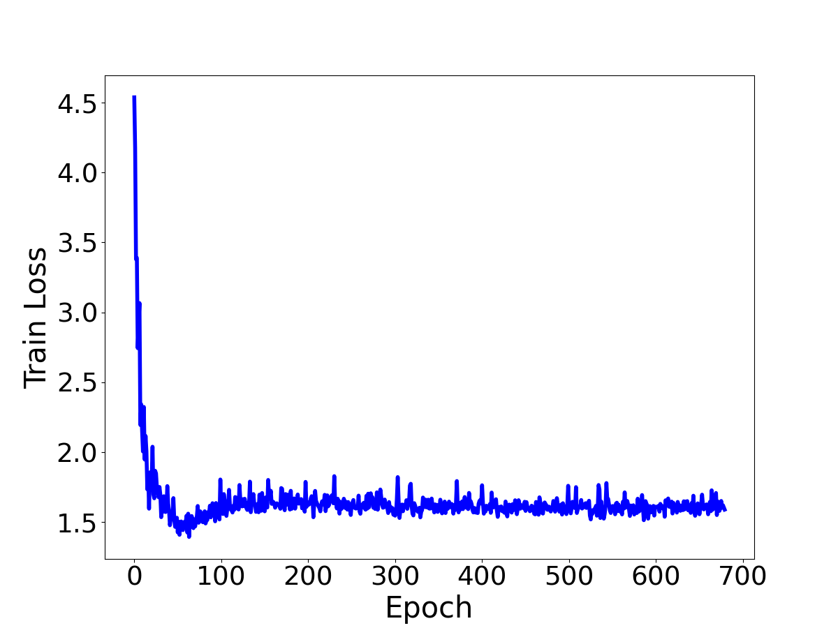
(b) The curve of training loss under A $\rightarrow$ P

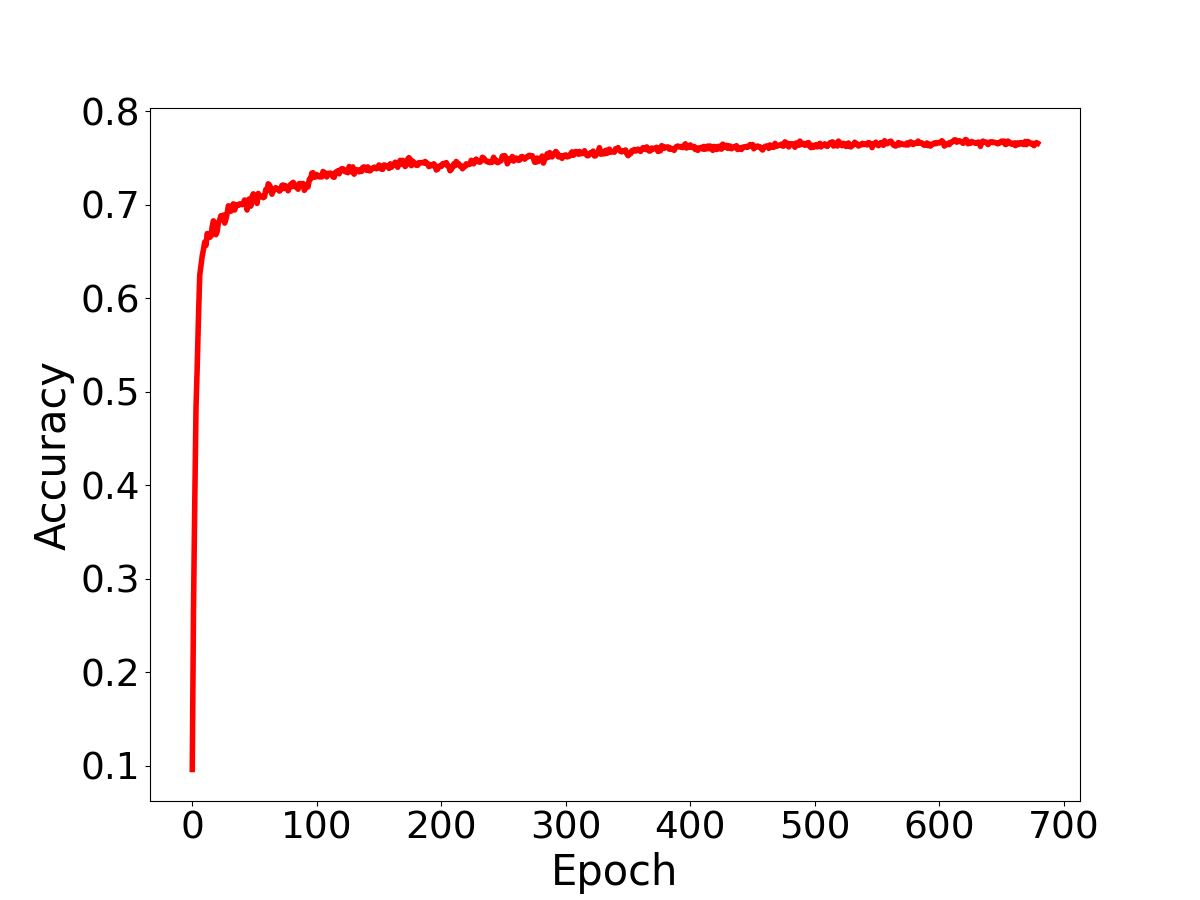
(c) The curve of accuracy under R $\rightarrow$ A

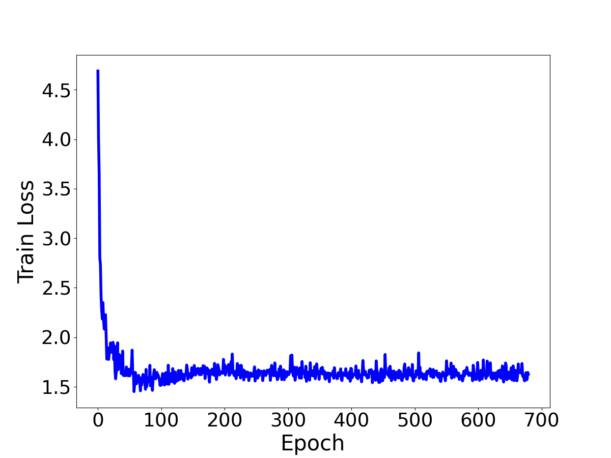
(d) The curve of training loss under R $\rightarrow$ A

Figure 8: Convergence. The red curve is the changes of accuracy during the training process and the blue curve is the changes of training loss. The experiments are conducted on OfficeHome dataset, where (a) and (b) are in A $\rightarrow$ P setting, (c) and (d) are in R $\rightarrow$ A setting.

References

- [1] Mustapha Aouchiche and Pierre Hansen. Distance spectra of graphs: a survey. Linear algebra and its applications, 458:301–386, 2014.
- [2] Eric Arazo, Diego Ortego, Paul Albert, Noel E O’Connor, and Kevin McGuinness. Pseudo-labeling and confirmation bias in deep semi-supervised learning. In International Joint Conference on Neural Networks (IJCNN). IEEE, 2020.
- [3] Shai Ben-David, John Blitzer, Koby Crammer, and Fernando Pereira. Analysis of representations for domain adaptation. In Advances in Neural Information Processing Systems (NeurIPS), volume 19, 2006.
- [4] Shai Ben-David, John Blitzer, Koby Crammer, and Fernando Pereira. Analysis of representationsfor domain adaptation. In Advances in Neural Information Processing Systems (NeurIPS), page 137–144, 2007.
- [5] David Berthelot, Nicholas Carlini, Ian J. Goodfellow, Nicolas Papernot, Avital Oliver, and Colin A Raffel. Mixmatch: A holistic approach to semi-supervised learning. In Advances in Neural Information Processing Systems (NeurIPS), volume 32, pages 5050–5060, 2019.
- [6] Andries E. Brouwer and Willem H. Haemers. Spectra of graphs. Springer Science and Business Media, 2011.
- [7] Joan Bruna, Wojciech Zaremba, Arthur Szlam, and Yann LeCun. Spectral networks and locally connected networks on graphs. In International Conference on Learning Representations (ICLR), 2014.
- [8] Lin Chen, Huaian Chen, Zhixiang Wei, Xin Jin, Xiao Tan, Yi Jin, and Enhong Chen. Reusing the task-specific classifier as a discriminator: Discriminator-free adversarial domain adaptation. In Proceedings of the IEEE Conference on Computer Vision and Pattern Recognition (CVPR), pages 7181–7190. IEEE, 2022.
- [9] Liqun Chen, Zhe Gan, Yu Cheng, Linjie Li, Lawrence Carin, and Jingjing Liu. Graph optimal transport for cross-domain alignment. In Proceedings of the 37th International Conference on Machine Learning (ICML), pages 1542–1553. PMLR, 2020.
- [10] Xinyang Chen, Sinan Wang, Mingsheng Long, and Jianmin Wang. Transferability vs. discriminability: Batch spectral penalization for adversarial domain adaptation. In Proceedings of the 36th International Conference on Machine Learning (ICML), pages 1081–1090. PMLR, 2019.
- [11] Yuhao Cheng, Xiaoguang Zhu, Jiuchao Qian, Fei Wen, and Peilin Liu. Cross-modal graph matching network for image-text retrieval. ACM Transactions on Multimedia Computing, Communications, and Applications, 18(4):1–23, 2022.
- [12] Fan RK Chung. Spectral graph theory. American Mathematical Society, 92, 1997.
- [13] Shuhao Cui, Shuhui Wang, Junbao Zhuo, Liang Li, Qingming Huang, and Qi Tian. Towards discriminability and diversity: Batch nuclear-norm maximization under label insufficient situations. In Proceedings of the IEEE Conference on Computer Vision and Pattern Recognition (CVPR), pages 3941–3950. IEEE, 2020.
- [14] Shuhao Cui, Shuhui Wang, Junbao Zhuo, Chi Su, Qingming Huang, and Qi Tian. Gradually vanishing bridge for adversarial domain adaptation. In Proceedings of the IEEE Conference on Computer Vision and Pattern Recognition (CVPR), pages 12452–12461. IEEE, 2020.
- [15] Shai Ben David, Tyler Lu, Teresa Luu, and David Pal. Impossibility theorems for domain adaptation. In Proceedings of the 13th International Conference on Artificial Intelligence and Statistics (AISTATS), pages 129–136. PMLR, 2010.
- [16] Michaël Defferrard, Xavier Bresson, and Pierre Vandergheynst. Convolutional neural networks on graphs with fast localized spectral filtering. In Advances in Neural Information Processing Systems (NeurIPS), volume 29, pages 3837–3845, 2016.
- [17] Laurens Van der Maaten and Geoffrey Hinton. Visualizing data using t-sne. The Journal of Machine Learning Research (JMLR), 9(11), 2008.
- [18] Yaroslav Ganin and Victor Lempitsky. Unsupervised domain adaptation by back propagation. In Proceedings of the 32th International Conference on Machine Learning (ICML), pages 1180–1189. PMLR, 2015.
- [19] Yaroslav Ganin, Evgeniya Ustinova, Hana Ajakan, Pascal Germain, Hugo Larochelle, François Laviolette, Mario Marchand, and Victor S. Lempitsky. Domain-adversarial training of neural networks. The Journal of Machine Learning Research (JMLR), 17:59:1–59:35, 2016.
- [20] Boqing Gong, Yuan Shi, Fei Sha, and Kristen Grauman. Geodesic flow kernel for unsupervised domain adaptation. In Proceedings of the IEEE Conference on Computer Vision and Pattern Recognition (CVPR), pages 2066–2073. IEEE, 2012.
- [21] Yves Grandvalet and Yoshua Bengio. Semi-supervised learning by entropy minimization. In Advances in Neural Information Processing Systems (NeurIPS), 2004.
- [22] Jiao Gu, Bobo Hua, and Shiping Liu. Spectral distances on graphs. Discrete Applied Mathematics, 190:56–74, 2015.
- [23] Xiang Gu, Jian Sun, and Zongben Xu. Spherical space domain adaptation with robust pseudo-label loss. In Proceedings of the IEEE Conference on Computer Vision and Pattern Recognition (CVPR), pages 9101–9110. IEEE, 2020.
- [24] Chuan Guo, Geoff Pleiss, Yu Sun, and Kilian Q. Weinberger. On calibration of modern neural networks. In Proceedings of the 34th International Conference on Machine Learning (ICML), pages 1321–1330. PMLR, 2017.
- [25] Kaiming He, Xiangyu Zhang, Shaoqing Ren, and Jian Sun. Deep residual learning for image recognition. In Proceedings of the IEEE Conference on Computer Vision and Pattern Recognition (CVPR), pages 770–778. IEEE, 2016.
- [26] Kaiming He, Xiangyu Zhang, Shaoqing Ren, and Jian Sun. Identity mappings in deep residual networks. In the 14th European Conference on Computer Vision (ECCV), volume 9908, pages 630–645. Springer, 2016.
- [27] Ahmet Iscen, Giorgos Tolias, Yannis Avrithis, and Ondrej Chum. Label propagation for deep semi-supervised learning. In Proceedings of the IEEE Conference on Computer Vision and Pattern Recognition (CVPR), pages 5070–5079. IEEE, 2019.
- [28] Junguang Jiang, Baixu Chen, Bo Fu, and Mingsheng Long. Transfer-learning-library. https://github.com/thuml/Transfer-Learning-Library, 2020.
- [29] Junguang Jiang, Yang Shu, Jianmin Wang, and Mingsheng Long. Transferability in deep learning: A survey. CoRR, abs/2201.05867, 2022.
- [30] Pin Jiang, Aming Wu, Yahong Han, Yunfeng Shao, Meiyu Qi, and Bingshuai Li. Bidirectional adversarial training for semi-supervised domain adaptation. In Proceedings of the 29th International Joint Conference on Artificial Intelligence (IJCAI), page 934–940, 2020.
- [31] Ying Jin, Ximei Wang, Mingsheng Long, and Jianmin Wang. Minimum class confusion for versatile domain adaptation. In the 16th European Conference on Computer Vision (ECCV), volume 12366, pages 464–480. Springer, 2020.
- [32] Quinonero-Candela Joaquin, Masashi Sugiyama, Anton Schwaighofer, and Neil D. Lawrence. Dataset shift in machine learning. Mit Press, 2008.
- [33] Tarun Kalluri, Astuti Sharma, and Manmohan Chandraker. Memsac: Memory augmented sample consistency for large scale domain adaptation. In the 17th European Conference on Computer Vision (ECCV), pages 550–568. Springer, 2022.
- [34] Andrej Karpathy and Fei-Fei Li. Deep visual-semantic alignments for generating image descriptions. In Proceedings of the IEEE Conference on Computer Vision and Pattern Recognition (CVPR), pages 3128–3137. IEEE, 2015.
- [35] Taekyung Kim and Changick Kim. Attract, perturb, and explore: Learning a feature alignment network for semisupervised domain adaptation. In the 16th European Conference on Computer Vision (ECCV), pages 591–607. Springer, 2020.
- [36] Thomas N. Kipf and Max Welling. Semi-supervised classification with graph convolutional networks. In International Conference on Learning Representations (ICLR), 2017.
- [37] Jogendra Nath Kundu, Suvaansh Bhambri, Akshay Kulkarni, Hiran Sarkar, Varun Jampani, and R. Venkatesh Babu. Subsidiary prototype alignment for universal domain adaptation. In Advances in Neural Information Processing Systems (NeurIPS), volume 35, 2022.
- [38] Jogendra Nath Kundu, Akshay R Kulkarni, Suvaansh Bhambri, Deepesh Mehta, Shreyas Anand Kulkarni, Varun Jampani, and Venkatesh Babu Radhakrishnan. Balancing discriminability and transferability for source-free domain adaptation. In Proceedings of the 39th International Conference on Machine Learning (ICML), volume 162, pages 11710–11728. PMLR, 2022.
- [39] Dong-Hyun Lee. Pseudo-label: The simple and efficient semi-supervised learning method for deep neural networks. In Workshop on challenges in representation learning, ICML, page 896, 2013.
- [40] Seungmin Lee, Dongwan Kim, Namil Kim, and Seong-Gyun Jeong. Drop to adapt: Learning discriminative features for unsupervised domain adaptation. In Proceedings of the IEEE International Conference on Computer Vision (ICCV), pages 91–100. IEEE, 2019.
- [41] Jichang Li, Guanbin Li, Yemin Shi, and Yizhou Yu. Cross-domain adaptive clustering for semi-supervised domain adaptation. In Proceedings of the IEEE Conference on Computer Vision and Pattern Recognition (CVPR), pages 2505–2514, 2021.
- [42] Jingjing Li, Erpeng Chen, Dingm Zhengming, Lei Zhy, Ke Lu, and Heng Tao Shen. Maximum density divergence for domain adaptation. IEEE transactions on pattern analysis and machine intelligence (TPAMI), 11(43):3918–3930, 2020.
- [43] Linjie Li, Zhe Gan, Yu Cheng, and Jingjing Liu. Relation-aware graph attention network for visual question answering. In Proceedings of the IEEE International Conference on Computer Vision (ICCV), pages 10312–10321. IEEE, 2019.
- [44] Mengxue Li, Yi-Ming Zhai, You-Wei Luo, Peng-Fei Ge, and Chuan-Xian Ren. Enhanced transport distance for unsupervised domain adaptation. In Proceedings of the IEEE conference on computer vision and pattern recognition (CVPR), pages 13936–13944. IEEE, 2020.
- [45] Shuang Li, Fangrui Lv, Binhui Xie, Chi Harold Liu, Jian Liang, and Chen Qin. Bi-classifier determinacy maximization for unsupervised domain adaptation. In Proceedings of 35th AAAI Conference on Artificial Intelligence, pages 8455–8464. AAAI Press, 2021.
- [46] Wuyang Li, Xinyu Liu, and Yixuan Yuan. SIGMA: semantic-complete graph matching for domain adaptive object detection. In Proceedings of the IEEE Conference on Computer Vision and Pattern Recognition (CVPR), pages 5281–5290. IEEE, 2022.
- [47] Jian Liang, Ran He, Zhenan Sun, and Tieniu Tan. Exploring uncertainty in pseudo-label guided unsupervised domain adaptation. Pattern Recognition, 96, 2019.
- [48] Jian Liang, Dapeng Hu, and Jiashi Feng. Domain adaptation with auxiliary target domain-oriented classifier. In Proceedings of the IEEE Conference on Computer Vision and Pattern Recognition (CVPR), pages 16632–16642. IEEE, 2021.
- [49] Tsung-Yi Lin, Michael Maire, Serge Belongie, Lubomir Bourdev, Ross Girshick, James Hays, Pietro Perona, Deva Ramanan, C. Lawrence Zitnick, and Piotr Dollár. Microsoft coco: Common objects in context. In the 13th European Conference on Computer Vision (ECCV), pages 740–755. Springer, 2014.
- [50] Yanbin Liu, Juho Lee, Minseop Park, Saehoon Kim, Eunho Yang, Sungju Hwang, and Yi Yang. Learning to propagate labels: Transductive propagation network for few-shot learning. In International Conference on Learning Representations (ICLR), 2019.
- [51] Mingsheng Long, Yue Cao, Jianmin Wang, and Michael I. Jordan. Learning transferable features with deep adaptation networks. In Proceedings of the 32th International Conference on Machine Learning (ICML), pages 97–105. PMLR, 2015.
- [52] Mingsheng Long, Zhangjie Cao, Jianmin Wang, and Michael I. Jordan. Conditional adversarial domain adaptation. In Advances in Neural Information Processing Systems (NeurIPS), volume 31, pages 1647–1657, 2018.
- [53] Mingsheng Long, Han Zhu, Jianmin Wang, and Michael I. Jordan. Deep transfer learning with joint adaptation networks. In Proceedings of the 34th International Conference on Machine Learning (ICML), pages 2208–2217. PMLR, 2017.
- [54] Lingkun Luo, Liming Chen, and Shiqiang Hu. Attention regularized laplace graphfor domain adaptation. In Proceedings of 31th IEEE International Conference on Image Processing (ICIP), pages 7322–7337. IEEE, 2022.
- [55] Miller McPherson, Lynn SmithLovin, and James M Cook. Birds of a feather: Homophily in social networks. Annual review of socialogy, 27(1):415–444, 2001.
- [56] Jaemin Na, Heechul Jung, Hyung Jin Chang, and Wonjun Hwang. Fixbi: Bridging domain spaces for unsupervised domain adaptation. In Proceedings of the IEEE Conference on Computer Vision and Pattern Recognition (CVPR), pages 1094–1103. IEEE, 2021.
- [57] Xingchao Peng, Qinxun Bai, Xide Xia, Zijun Huang, Kate Saenko, and Bo Wang. Moment matching for multi-source domain adaptation. In Proceedings of the IEEE International Conference on Computer Vision (ICCV), pages 1406–1415. IEEE, 2019.
- [58] Xingchao Peng, Ben Usman, Neela Kaushik, Dequan Wang, Judy Hoffman, and Kate Saenko. Visda: A synthetic-to-real benchmark for visual domain adaptation. In Proceedings of the IEEE Conference on Computer Vision and Pattern Recognition Workshops (CVPR Workshops), pages 2021–2026. IEEE, 2018.
- [59] Hieu Pham, Zihang Dai, Qizhe Xie, and Quoc V. Le. Meta pseudo labels. In Proceedings of the IEEE Conference on Computer Vision and Pattern Recognition (CVPR), pages 11557–11568. IEEE, 2021.
- [60] Zhenyu Qiu, Wenbin Hu, Jia Wu, ZhongZheng Tang, and Xiaohua Jia. Noise-resilient similarity preserving network embedding for social networks. In Proceedings of the 28nd International Joint Conference on Artificial Intelligence (IJCAI), pages 3282–3288, 2019.
- [61] Md Mahmudur Rahman, Rameswar Panda, and Mohammad Arif Ul Alam. Semi-supervised domain adaptation with auto-encoder via simultaneous learning. Proceedings of the IEEE Winter Conference on Applications of Computer Vision, 2023.
- [62] Harsh Rangwani, Sumukh K Aithal, Mayank Mishra, Arihant Jain, and R. Venkatesh Babu. A closer look at smoothness in domain adversarial training. In Proceedings of the 39th International Conference on Machine Learning (ICML). PMLR, 2022.
- [63] Kate Saenko, Brian Kulis, Mario Fritz, and Trevor Darrell. Adapting visual category models to new domains. In the 11th European Conference on Computer Vision (ECCV), pages 213–226. Springer, 2010.
- [64] Kuniaki Saito, Donghyun Kim, Stan Sclaroff, Trevor Darrell, and Kate Saenko. Semi-supervised domain adaptation via minimax entropy. Proceedings of the IEEE International Conference on Computer Vision (ICCV), pages 8050–8058, 2019.
- [65] Kuniaki Saito, Donghyun Kim, Stan Sclaroff, and Kate Saenko. Universal domain adaptation through self supervision. In Advances in Neural Information Processing Systems (NeurIPS), volume 33, 2020.
- [66] Kuniaki Saito, Kohei Watanabe, Yoshitaka Ushiku, and Tatsuya Harada. Maximum classifier discrepancy for unsupervised domain adaptation. In Proceedings of the IEEE Conference on Computer Vision and Pattern Recognition (CVPR), pages 3723–3732. IEEE, 2018.
- [67] Hidetoshi Shimodaira. Improving predictive inference under covariate shift by weighting the log-likelihood function. Journal of Statistical Planning and Inference, 90(2):227––244, 2000.
- [68] Tiberiu Sosea and Cornelia Caragea. Leveraging training dynamics and self-training for text classification. In Findings of the Association for Computational Linguistics: EMNLP, pages 4750–4762. ACL, 2022.
- [69] Dragan Stevanović. Research problems from the aveiro workshop on graph spectra. Linear Algebra and its Applications, 423(1):172–181, 2007. Special Issue devoted to papers presented at the Aveiro Workshop on Graph Spectra.
- [70] Baochen Sun and Kate Saenko. Deep coral: Correlation alignment for deep domain adaptation. In ECCV 2016 Workshops, 2016.
- [71] Christian Szegedy, Vincent Vanhoucke, Sergey Ioffe, Jonathon Shlens, and Zbigniew Wojna. Rethinking the inception architecture for computer vision. In Proceedings of the IEEE Conference on Computer Vision and Pattern Recognition (CVPR), pages 2818–2826. IEEE, 2016.
- [72] Tatiana Tommasi, Martina Lanzi, Paolo Russo, and Barbara Caputo. Learning the roots of visual domain shift. In Gang Hua and Hervé Jégou, editors, ECCV 2016 Workshops, volume 9915 of Lecture Notes in Computer Science, pages 475–482, 2016.
- [73] Eric Tzeng, Judy Hoffman, Kate Saenko, and Trevor Darrell. Adversarial discriminative domain adaptation. In Proceedings of the IEEE Conference on Computer Vision and Pattern Recognition (CVPR), pages 2962–2971. IEEE, 2017.
- [74] Varun Vasudevan, Maxime Bassenne, Md Tauhidul Islam, and Lei Xing. Image classification using graph neural network and multiscale wavelet superpixels. Pattern Recognition Letters, 166:89–96, 2023.
- [75] Petar Veličković, Guillem Cucurull, Arantxa Casanova, Adriana Romero, Pietro Liò, and Yoshua Bengio. Graph attention networks. International Conference on Learning Representations (ICLR), 2018.
- [76] Hemanth Venkateswara, Jose Eusebio, Shayok Chakraborty, and Sethuraman Panchanathan. Deep hashing network for unsupervised domain adaptation. In Proceedings of the IEEE Conference on Computer Vision and Pattern Recognition (CVPR), pages 5018–5027. IEEE, 2017.
- [77] Ulrike von Luxburg. A tutorial on spectral clustering. Statistics and Computing, 17(4):395–416, 2007.
- [78] Bo Wang, Armin Pourshafeie, Marinka Zitnik, Junjie Zhu, Carlos D Bustamante, Serafim Batzoglou, and Jure Leskovec. Network enhancement as a general method to denoise weighted biological networks. Nature communications, 9(1):1–8, 2018.
- [79] Sinan Wang, Xinyang Chen, Yunbo Wang, Mingsheng Long, and Jianmin Wang. Progressive adversarial networks for fine-grained domain adaptation. In Proceedings of the IEEE conference on computer vision and pattern recognition (CVPR), pages 9213–9222, 2020.
- [80] Xiaodong Wang, Junbao Zhuo, Mengru Zhang, Shuhui Wang, and Yuejian Fang. Revisiting unsupervised domain adaptation models: a smoothness perspective. In Proceedings of the Asian Conference on Computer Vision (ACCV), pages 1504–1521, 2022.
- [81] Yuxi Wang, Junran Peng, and ZhaoXiang Zhang. Uncertainty-aware pseudo label refinery for domain adaptive semantic segmentation. In Proceedings of the IEEE International Conference on Computer Vision (ICCV), pages 9092–9101. IEEE, 2021.
- [82] Guoqiang Wei, Cuiling Lan, Wenjun Zeng, and Zhibo Chen. Metaalign: Coordinating domain alignment and classification for unsupervised domain adaptation. In Proceedings of the IEEE Conference on Computer Vision and Pattern Recognition (CVPR), pages 16643–16653. IEEE, 2021.
- [83] Zhirong Wu, Yuanjun Xiong, Stella Yu, and Dahua Lin. Unsupervised feature learning via non-parametric instancediscrimination. In Proceedings of the IEEE Conference on Computer Vision and Pattern Recognition (CVPR), pages 3733–3742. IEEE, 2018.
- [84] Sang Michael Xie, Ananya Kumar, Robbie Jones, Fereshte Khani, Tengyu Ma, and Percy Liang. In-n-out: Pre-training and self-training using auxiliary information for out-of-distribution robustness. In International Conference on Learning Representations (ICLR), 2021.
- [85] Ruijia Xu, Guanbin Li, Jihan Yang, and Liang Lin. Larger norm more transferable: An adaptive feature norm approach for unsupervised domain adaptation. In Proceedings of the IEEE International Conference on Computer Vision (ICCV), pages 1426–1435, 2019.
- [86] Rex Ying, Ruining He, Kaifeng Chen, Pong Eksombatchai, William L. Hamilton, and Jure Leskovec. Graph convolutional neural networks for web-scale recommender systems. In Proceedings of the 24th ACM SIGKDD International Conference on Knowledge Discovery and Data Mining., pages 974–983. ACM, 2018.
- [87] Yue Zhang, Shun Miao, and Rui Liao. Structural domain adaptation with latent graph alignment. In Proceedings of 25th IEEE International Conference on Image Processing (ICIP), pages 3753–3757. IEEE, 2018.
- [88] Zijun Zhang, Xiao Cao, Yuan Liu, and Mingsheng Long. Progressive graph learning for open-set domain adaptation. In Proceedings of the 37th International Conference on Machine Learning (ICML), pages 6468–6478. PMLR, 2020.
- [89] Erheng Zhong, Wei Fan, Qiang Yang, Olivier Verscheure, and Jiangtao Ren. Cross validation framework to choose amongst models and datasets for transfer learning. In Machine Learning and Knowledge Discovery in Databases, European Conference, ECML PKDD, volume 6323 of Lecture Notes in Computer Science, pages 547–562. Springer, 2010.
- [90] Fuzhen Zhuang, Zhiyuan Qi, Keyu Duan, Dongbo Xi, Yongchun Zhu, Hengshu Zhu, Hui Xiong, and Qing He. A comprehensive survey on transfer learning. Proceedings of the IEEE, 109(1):43–76, 2021.
- [91] Zhijian Zhuo, Yifei Wang, Jinwen Ma, and Yisen Wang. Towards a unified theoretical understanding of non-contrastive learning via rank differential mechanism. In International Conference on Learning Representations (ICLR), 2023.