Scalar Cosmological Perturbations from Quantum Gravitational Entanglement

Abstract

A major challenge at the interface of quantum gravity and cosmology is to explain how the large-scale structure of the Universe emerges from physics at the Planck scale. In this letter, we take an important step in this direction by extracting the dynamics of scalar isotropic cosmological perturbations from full quantum gravity, as described by the causally complete Barrett-Crane group field theory model. From the perspective of the underlying quantum gravity theory, cosmological perturbations are represented as nearest-neighbor two-body entanglement of group field theory quanta. Their effective dynamics is obtained via mean-field methods and described relationally with respect to a physical Lorentz frame causally coupled to the quantum geometry. We quantitatively study these effective dynamical equations and show that at low energies they are perfectly consistent with those of General Relativity, while for trans-Planckian scales quantum effects become important. These results therefore not only provide crucial insights into the potentially purely quantum gravitational nature of cosmological perturbations, but also offer rich phenomenological implications for the physics of the early Universe.

The extraction of cosmology from full quantum gravity (QG) constitutes a fundamental objective shared across all quantum gravity approaches Blumenhagen et al. (2013); Percacci (2017); Reuter and Saueressig (2019); Bonanno et al. (2020); Ambjorn et al. (2012); Hamber (2009); Surya (2019); Rovelli (2004, 2011); Perez (2013); Asante et al. (2022); Ashtekar and Lewandowski (2004); Thiemann (2007); Freidel (2005); Oriti (2011); Carrozza (2013); Gurau (2016a, b). This endeavor holds the promise of addressing longstanding open questions of the $\Lambda$CDM model Aghanim et al. (2020), in particular concerning the origin of primordial perturbations, and subjecting quantum gravity theories to the testing ground of cosmological observations. Achieving this goal, however, presents a formidable challenge, particularly in approaches with fundamentally discrete geometric degrees of freedom that differ significantly from the continuum gravitational field at the heart of standard cosmology. This challenge involves the definition of a robust coarse-graining procedure to identify macroscopic geometric and matter degrees of freedom, and to define time evolution and spatiotemporal localization in the absence of a conventional spacetime manifold.

Group field theories (GFTs) Freidel (2005); Oriti (2006, 2011) provide a rich and versatile framework to tackle both of these challenges. They are non-local quantum field theories of spacetime, the fundamental excitations of which correspond to discrete quantum geometric building blocks. GFTs are closely related to other QG approaches such as loop quantum gravity Oriti (2016); Ashtekar and Lewandowski (2004), spin foam models Perez (2013), simplicial lattice gravity Bonzom (2009); Baratin and Oriti (2012, 2011) and dynamical triangulations Ambjorn et al. (2012); Loll (2020, 1998).

Spatially homogeneous and flat cosmological dynamics have been successfully recovered from the mean-field dynamics of GFT condensate states Gielen et al. (2013, 2014); Oriti et al. (2016); Gielen and Sindoni (2016); Pithis and Sakellariadou (2019); Marchetti and Oriti (2021a); Jercher et al. (2022a), representing the simplest form of coarse-graining of the underlying quantum gravitational dynamics. The existence of such states has recently been supported by a Landau-Ginzburg mean-field analysis of Lorentzian GFTs Marchetti et al. (2023a, b). Moreover, a special class of condensate states, called coherent peaked states (CPSs) Marchetti and Oriti (2021b, a, 2022), provides a solution to the aforementioned localization problem by allowing the construction of effective relational observables.

Deriving the dynamics of cosmological perturbations from GFTs has been commenced in Gielen and Oriti (2018); Gielen (2019); Gerhardt et al. (2018); Gielen and Mickel (2023) and in particular pushed forward in Marchetti and Oriti (2022), where the classical perturbation equations of General Relativity (GR) have been recovered in the super-horizon limit of large perturbation wavelengths. However, deviations from classical results occur there for non-negligible wave vectors, which we here argue to arise from an insufficient coupling between the physical reference frame and the underlying causal structure.

In this letter, we advance this program and derive cosmological perturbation equations from GFT quantum gravity that agree with classical results at sub-Planckian scales and are subject to quantum corrections in the trans-Planckian regime. This is achieved by: (i) utilizing the rich causal structure of the completion Jercher et al. (2022a, b) of Barrett-Crane (BC) GFT model Barrett and Crane (2000); Perez and Rovelli (2001a, b) to causally couple for the first time a physical Lorentzian reference frame to the GFT model; and (ii) encoding inhomogeneities of cosmological observables as the (relational) nearest-neighbor two-body entanglement of microscopic degrees of freedom, hence concretely realizing the general expectation that non-trivial geometries are associated with quantum gravitational entanglement Ryu and Takayanagi (2006); Bianchi and Myers (2014); Cao et al. (2017); Swingle (2018); Colafrancheschi (2022).

I The BC model with Lorentzian Frame

In this letter, we consider a minimal extension of the BC GFT model based on spacelike ($+$) and timelike ($-$) tetrahedra Jercher et al. (2022b), which is described by two fields $\varphi_{\pm}\equiv\varphi(g_{v},X_{\alpha},\boldsymbol{\Phi})$ with $\alpha\in\{+,-\}$. Here, $g_{v}=(g_{1},g_{2},g_{3},g_{4})\in\text{SL$(2,\mathbb{C})$}^{4}$ and $X_{\alpha}\in\text{SL$(2,\mathbb{C})$}/\mathrm{U}^{(\alpha)}$ is a normal vector, where $\mathrm{U}^{(+)}=\mathrm{SU}(2)$ and $\mathrm{U}^{(-)}=\mathrm{SU}(1,1)$. Finally, $\boldsymbol{\Phi}=(\phi_{1},\dots,\phi_{n})\in\mathbb{R}^{n}$ represents $n$ minimally coupled free massless scalar fields Li et al. (2017). Closure and simplicity constraints are imposed by requiring the fields $\varphi_{\pm}$ to satisfy

$$\varphi(g_{v},X_{\alpha}) =\varphi(g_{v}h^{-1},h\cdot X_{\alpha}),\quad\forall h\in\text{SL$(2,\mathbb{C})$},$$ (1)

$$\varphi(g_{v},X_{\alpha}) =\varphi(g_{v}u_{v},X_{\alpha}),\quad\forall u_{1},...,u_{4}\in\mathrm{U}_{X_{\alpha}},$$ (2)

respectively, where $\mathrm{U}_{X_{\alpha}}\simeq\mathrm{U}^{(\alpha)}$ is $X_{\alpha}$-stabilizer subgroup of SL$(2,\mathbb{C})$. In bi-vector representation, the geometric interpretation of the fields as spacelike and timelike tetrahedra becomes transparent Jercher et al. (2022b).

The dynamics of the model are specified by an action $S[\bar{\varphi},\varphi]=K[\bar{\varphi},\varphi]+V[\bar{\varphi},\varphi]$, where $K$ and $V$ represent kinetic and interaction terms. In particular, $K=K_{+}+K_{-}$, with

$$K_{\pm}=\bar{\varphi}_{\pm}\cdot\mathcal{K}^{(X)}_{\pm}\cdot\varphi_{\pm}\,,$$ (3)

where $\cdot$ represents an integration over the full GFT field domain $\text{SL$(2,\mathbb{C})$}^{4}\times\text{SL$(2,\mathbb{C})$}/\mathrm{U}^{(\alpha)}\times\mathbb{R}^{n}$. The kinetic kernels

$$\mathcal{K}^{(X)}_{\pm}=\delta(X^{(v)}_{\pm}-X^{(w)}_{\pm})\mathcal{K}_{\pm}(g_{v},g_{w};\Delta_{vw}^{2}\boldsymbol{\Phi})\,,$$ (4)

where $\Delta^{2}_{vw}\boldsymbol{\Phi}\equiv((\phi_{1,v}-\phi_{1,w})^{2},\dots,(\phi_{n,v}-\phi_{n,w})^{2})$, encode information about the propagation of geometry and matter data between neighbouring tetrahedra (denoted $v$ and $w$) and clearly show that the $X_{\alpha}$ are non-dynamical. For further details, see Jercher et al. .

The interaction $V$ is non-local in the group theoretic variables and represents any possible gluing of five tetrahedra with arbitrary signature to form a $4$-simplex. Scalar fields $\boldsymbol{\Phi}$ are discretized on dual vertices and therefore enter as local data in the interaction kernel Li et al. (2017).

The Fock space $\mathcal{F}$ of the model can be constructed by tensoring the Fock spaces associated to the two different sectors, i.e. $\mathcal{F}\equiv\mathcal{F}_{+}\otimes\mathcal{F}_{-}$, with

$$\mathcal{F}_{\pm}\equiv\bigoplus_{N=0}^{\infty}\mathrm{sym}\left(\mathcal{H}_{\pm}^{(1)}\otimes...\otimes\mathcal{H}_{\pm}^{(N)}\right),$$ (5)

constructed out of the one-particle Hilbert spaces,

$$\mathcal{H}_{\pm}\equiv L^{2}\left(\text{SL$(2,\mathbb{C})$}^{4}\times\text{SL$(2,\mathbb{C})$}/\mathrm{U}^{(\pm)}/\sim_{\pm}\right).$$ (6)

The $\mathcal{F}_{\pm}$ can be generated by repeated action of the creation operator $\hat{\varphi}^{\dagger}_{\pm}\equiv\hat{\varphi}^{\dagger}_{\pm}\otimes\mathbbm{1}_{\mp}$ on the Fock vacua $\ket{\emptyset}_{\pm}$ annihilated by $\hat{\varphi}_{\pm}$. Creation and annihilation operators satisfy

$$\commutator{\hat{\varphi}_{\pm}(\boldsymbol{\Phi})}{\hat{\varphi}_{\pm}^{\dagger}(\boldsymbol{\Phi}^{\prime})}=\delta^{(n)}(\boldsymbol{\Phi}-\boldsymbol{\Phi}^{\prime})\mathbbm{1}_{\pm}\,,$$ (7)

where $\mathbbm{1}_{\pm}$ represents the identity on $\mathcal{F}_{\pm}$ satisfying closure and simplicity constraints, and where we have left explicit only the matter field dependence for simplicity.

From here on, we focus on $n=5$ scalar fields, out of which $4$ (denoted by $\chi^{\mu}$ with $\mu\in\{0,...,3\}$) will be used to construct a physical Lorentzian reference frame, allowing us to describe the system in a relational manner. More precisely, $\chi^{0}$ serves as a relational clock and $\chi^{i}$ with $i\in\{1,2,3\}$ serve as relational rods. The remaining scalar field $\phi$ will be assumed to dominate the energy-momentum budget of the system, being slightly inhomogeneous with respect to the rods.

Importantly, the manifestly causal nature of the minimally extended BC GFT model allows us, for the first time, to consistently implement the Lorentzian properties of the physical frame at the QG level. Indeed, at a classical, discrete geometric level, a clock propagates along timelike dual edges, while rods propagate along spacelike dual edges. These conditions can be imposed strongly at the quantum gravity level by requiring that

$$\mathcal{K}_{+} =\mathcal{K}_{+}\bigl{(}g_{v},g_{w};(\chi^{0}_{v}-\chi^{0}_{w})^{2},(\phi_{v}-\phi_{w})^{2}\bigr{)},$$ (8a)

$$\mathcal{K}_{-} =\mathcal{K}_{-}\bigl{(}g_{v},g_{w};\absolutevalue{{\bf\it\chi}_{v}-{\bf\it\chi}_{w}}^{2},(\phi_{v}-\phi_{w})^{2}\bigr{)}.$$ (8b)

Note that no such restriction is assumed for the matter field $\phi$.

II Entangled coherent peaked states

Building on a series of previous results Oriti et al. (2016); Marchetti and Oriti (2021a); Jercher et al. (2022a) connecting coherent states to macroscopic cosmological geometries, in this letter we suggest that the dynamics of scalar cosmological perturbations can be extracted from the above quantum gravity model by considering states of the form

$$\ket{\Delta;x^{0},{\bf\it x}}=\mathcal{N}_{\Delta}e^{\hat{\sigma}\otimes\mathbbm{1}_{-}+\mathbbm{1}_{+}\otimes\hat{\tau}+\hat{\delta\Phi}\otimes\mathbbm{1}_{-}+\hat{\delta\Psi}+\mathbbm{1}_{+}\otimes\hat{\delta\Xi}}\ket{\emptyset},$$ (9)

where $\mathcal{N}_{\Delta}$ is a normalization factor and $\ket{\emptyset}=\ket{\emptyset}_{+}\otimes\ket{\emptyset}_{-}$ is the $\mathcal{F}$-vacuum. In the above expression,

$$\hat{\sigma}\equiv\sigma_{{\bf\it\xi}_{+};x^{0},p_{\phi}}\cdot\hat{\varphi}^{\dagger}_{+},\qquad\hat{\tau}\equiv\tau_{{\bf\it\xi}_{-};x^{0},{\bf\it x},p_{\phi}}\cdot\hat{\varphi}^{\dagger}_{-},$$ (10)

generate a background condensate state in the extended Fock space of the form

$$\ket{\sigma;x^{0},p_{\phi}}\otimes\ket{\tau;x^{0},{\bf\it x},p_{\phi}}=\mathcal{N}_{\sigma}\mathcal{N}_{\tau}\textrm{e}^{\hat{\sigma}\otimes\mathbbm{1}+\mathbbm{1}\otimes\hat{\tau}}\ket{\emptyset},$$ (11)

with $\ket{\sigma;x^{0},p_{\phi}}$ and $\ket{\tau;x^{0},{\bf\it x},p_{\phi}}$ representing spacelike and timelike condensates, respectively. The spacelike $\sigma_{{\bf\it\xi}_{+};x^{0},p_{\phi}}$ and timelike $\tau_{{\bf\it\xi}_{-};x^{0},{\bf\it x},p_{\phi}}$ condensate wavefunctions are localized around $\chi^{0}=x^{0}$ and $\chi^{0}=x^{0},{\bf\it\chi}={\bf\it x}$, respectively. Furthermore, they are similarly localized in $\phi$-Fourier space ($\phi\rightarrow\pi_{\phi}$) around an arbitrary scalar field momentum $p_{\phi}$. In practice, this is achieved by assuming that they both factorize into fixed (Gaussian, see Marchetti and Oriti (2022)) peaking functions and into reduced condensate wavefunctions, $\tilde{\sigma}$ and $\tilde{\tau}$, respectively. The peaking properties of the states are collectively represented by the multi-labels ${\bf\it\xi}_{+}=(\epsilon^{+},\pi_{0}^{+},\delta_{\pi})$ and ${\bf\it\xi}_{-}=(\epsilon^{-},\pi_{0}^{-},\delta,\pi_{x},\delta_{\pi})$, respectively, the meaning of which is explained in Jercher et al. (2023).

Requiring $\tilde{\sigma}$ (resp. $\tilde{\tau}$) to contain only gauge-invariant data, the spacelike (resp. timelike) condensate wavefunction can be seen as a distribution of geometric and matter data on a $3$–surface (resp. $(2+1)$–surface) localized at relational time $x^{0}$ (resp. relational point $(x^{0},{\bf\it x}))$. Therefore, averages of operators on such relationally localized states can be seen as effective relational observables Marchetti and Oriti (2021a). Relational homogeneity of the background structures is then imposed by assuming that $\tilde{\sigma}$ and $\tilde{\tau}$ only depend on the clock variable $\chi^{0}$. Furthermore, isotropy is imposed by requiring $\tilde{\sigma}$ and $\tilde{\tau}$ to depend only on a single spacelike representation label $\rho\in\mathbb{R}$. Under these assumptions, we have $\tilde{\sigma}=\tilde{\sigma}_{\rho}(\chi^{0},\pi_{\phi})$ and $\tilde{\tau}=\tilde{\tau}_{\rho}(\chi^{0},\pi_{\phi})$.

Inhomogeneities are encoded in (9) at the level of the operators $\hat{\delta\Phi}\otimes\mathbbm{1}_{-},\hat{\delta\Psi},$ and $\mathbbm{1}_{+}\otimes\hat{\delta\Xi}$. These are in general $n$-body operators, with $n>1$, and produce quantum entanglement within and between the spacelike and timelike sectors. From now on we will consider $\hat{\delta\Phi}$, $\hat{\delta\Psi}$ and $\hat{\delta\Xi}$ to be $2$-body operators:

$$\hat{\delta\Phi} =\hat{\varphi}^{\dagger}_{+}\cdot\delta\Phi\cdot\hat{\varphi}^{\dagger}_{+},$$ (12a)

$$\hat{\delta\Psi} =\hat{\varphi}^{\dagger}_{+}\cdot\delta\Psi\cdot\hat{\varphi}^{\dagger}_{-},$$ (12b)

$$\hat{\delta\Xi} =\hat{\varphi}^{\dagger}_{-}\cdot\delta\Xi\cdot\hat{\varphi}^{\dagger}_{-}\,.$$ (12c)

The kernels $\delta\Phi$, $\delta\Psi$ and $\delta\Xi$ are in general bi-local, non-factorized (hence entangling) functions of the respective GFT field domains. Imposing isotropy and gauge-invariance, the kernels take the form $\delta\Psi=\delta\Psi_{\rho_{v}\rho_{w}}(\chi^{\mu}_{v},\chi^{\mu}_{w},\phi_{v},\phi_{w})$, similarly for $\delta\Phi$ and $\delta\Xi$.

As we will see explicitly below, the above kernels, together with the reduced condensate wavefunctions, describe slightly inhomogeneous cosmological geometries. Their dynamics are derived via a mean-field approximation of the full quantum dynamics, i.e.

$$\expectationvalue{\functionalderivative{S[\hat{\varphi}_{\pm},\hat{\varphi_{\pm}}^{\dagger}]}{\hat{\varphi}(g_{v},X_{\pm},x^{\mu},\phi)}}{\Delta;x^{0},{\bf\it x}}=0.$$ (13)

From here on we restrict ourselves to a mesoscopic regime of negligible GFT interactions Oriti et al. (2016); Marchetti and Oriti (2021a) where only a single representation label $\rho_{o}$ dominates Gielen (2016); Jercher et al. (2022a). Thus, we will suppress any explicit dependence of functions on representation labels. Finally, since we are interested in small inhomogeneities represented by the kernels in (12), we study the mean-field equations (13) perturbatively by working with linearized states

$$\ket{\Delta;x^{0},{\bf\it x}}\approx\mathcal{N}_{\Delta}\left(\mathbbm{1}+\hat{\delta\Phi}+\hat{\delta\Psi}+\hat{\delta\Xi}\right)e^{\hat{\sigma}\otimes\mathbbm{1}_{-}+\mathbbm{1}_{+}\otimes\hat{\tau}}\ket{\emptyset}.$$ (14)

Neglecting interactions and simultaneously working perturbatively collapses the whole set of Schwinger-Dyson equations to the lowest order equations (13), see Jercher et al. (2023). As we will discuss below, this will result in a dynamical freedom at the level of perturbations.

At the background level, and in the limit of negligible interactions, equations for the spacelike and timelike sectors exactly decouple. Following from the peaking in $\pi_{\phi}$ and in the frame variables, the equations of motion of the spacelike $\tilde{\sigma}$ and timelike $\tilde{\tau}$ reduced condensate wavefunctions become second order differential equations in relational time. In the limit in which the modulus of these reduced condensate wavefunctions is large (associated with late relational times and classical behavior, see Oriti et al. (2016); Pithis and Sakellariadou (2017); Marchetti and Oriti (2021b)), solutions to the equations of motion are given by

$$\tilde{\sigma}(x^{0},p_{\phi}) =\tilde{\sigma}_{0}\textrm{e}^{(\mu_{+}+i\tilde{\pi}_{0}^{+})x^{0}},$$ (15a)

$$\tilde{\tau}(x^{0},p_{\phi}) =\tilde{\tau}_{0}\textrm{e}^{(\mu_{-}+i\tilde{\pi}_{0}^{-})x^{0}},$$ (15b)

where $\mu_{\pm}=\mu_{\pm}(p_{\phi})$ are in general functions of the peaking value of the matter field momentum.

At first order in perturbations, we obtain two differential equations for the three kernels $\delta\Psi$, $\delta\Phi$ and $\delta\Xi$. This dynamical freedom cannot be reduced beyond mean-field as long as interactions are negligible and the above kernels are small. However, it can be completely fixed by requiring a low-energy agreement with classical physics, as will be seen below. We parametrize this freedom by

$$\delta\Phi(\chi^{\mu},\pi_{\phi})=\mathrm{f}(\chi^{\mu})\delta\Psi(\chi^{\mu},\pi_{\phi}),$$ (16)

with the complex function $\mathrm{f}$ given by

$$\mathrm{f}(\chi^{0},{\bf\it\chi})=f(\chi^{0})\textrm{e}^{i\theta_{f}(\chi^{0})}\absolutevalue{\eta_{\delta}(\absolutevalue{{\bf\it\chi}-{\bf\it x}})}\textrm{e}^{2i\pi_{0}^{+}\chi^{0}},$$ (17)

where $f$ and $\theta_{f}$ are arbitrary real functions of $\chi^{0}$ and $\eta_{\delta}$ is a Gaussian peaking function with width $\delta$. Moreover, from now on, we consider correlations that belong to the same relationally localized $4$-simplex and are $\pi_{\phi}$-conserving, i.e.

$$\delta\Psi=\delta\Psi(\chi^{\mu},\pi_{\phi})\delta^{(4)}(\chi^{\mu}-\chi^{\prime\mu})\delta(\pi_{\phi}-\pi_{\phi}^{\prime}).$$ (18)

Setting $\epsilon^{+}=\epsilon^{-}$, $\pi_{0}^{+}=-\pi_{0}^{-},$ the perturbation equations simplify considerably. In particular, the kernel $\delta\Psi$ entangling timelike and spacelike sectors, satisfies an equation of the form

$$0=\delta\Psi^{\prime\prime}+t_{1}\delta\Psi^{\prime}+t_{0}\delta\Psi+s_{2}\nabla_{{\bf\it x}}^{2}\delta\Psi,$$ (19)

where primes denote relational time derivatives and $t_{i}\equiv t_{i}[f,\theta_{f}](x^{0},p_{\phi})$ and $s_{2}[f,\theta_{f}](x^{0},p_{\phi})$ are complex quantities depending on the functions $f$ and $\theta_{f}$.

III Effective dynamics of cosmological scalar perturbations

As mentioned above, at late times, quantum fluctuations of extensive operators acting on Fock space $\mathcal{F}$ are small Marchetti and Oriti (2021b). In this regime, which we consider from here on, one can to associate classical cosmological quantities $\mathcal{O}$ with expectation values of appropriate one-body GFT operators $\hat{\mathcal{O}}$ on the states (14), defined as

$$\mathcal{O}(x^{0},{\bf\it x}) \equiv\expectationvalue{\hat{\mathcal{O}}}{\Delta;x^{0},{\bf\it x}}$$

$$=\bar{\mathcal{O}}(x^{0})+\delta\mathcal{O}(x^{0},{\bf\it x}).$$ (20)

The above expectation value is effectively localized in relational spacetime, and thus should be compared to a corresponding classical relational Goeller et al. (2022) (or, equivalently, harmonic gauge-fixed) observable Gielen (2018). By construction, (III) splits into a background, $\bar{\mathcal{O}}$, and a perturbation, $\delta\mathcal{O}$.

A crucial example of such operators is the spatial $3$-volume $\hat{V}$ Oriti et al. (2016), the expectation value of which splits into $\bar{V}(x^{0},p_{\phi})=v\absolutevalue{\tilde{\sigma}(x^{0},p_{\phi})}^{2}$ and

$$\delta V(x^{0},p_{\phi})=2v\real\{F[\delta\Psi](x^{\mu},p_{\phi})\}]\,,$$ (21)

where $v$ is a volume eigenvalue Jercher et al. (2022a) scaling as $v\sim\rho_{o}^{3/2}$ and $F$ is a functional depending on background wavefunctions as well as the functions $f$ and $\theta_{f}$. The background volume satisfies

$$\frac{\bar{V}^{\prime}}{3\bar{V}}=\frac{2}{3}\mu_{+}(p_{\phi}),\qquad\left(\frac{\bar{V}^{\prime}}{3\bar{V}}\right)^{\prime}=0,$$ (22)

which matches classical flat Friedmann dynamics in harmonic gauge if $\mu_{+}(p_{\phi})=3\bar{\pi}_{\phi}/(8M_{\mathrm{Pl}}^{2})$ Oriti et al. (2016); de Cesare and Sakellariadou (2017); Marchetti and Oriti (2022). Since the spacelike and timelike sector decouple at background level, contributions of timelike tetrahedra drop out for spacelike observables.

A similar matching can be performed for the perturbations by rewriting $\delta\Psi=Re^{i\Theta}$ and fixing $\Theta=n\pi/2$, $\theta_{f}=\frac{\pi}{2}+2\tilde{\pi}_{0}^{+}x^{0}$ and

$$f=-\alpha a^{-4}\frac{\tilde{\tau}_{0}}{\tilde{\sigma}_{0}}\textrm{e}^{(\mu_{-}-\mu_{+})x^{0}},$$ (23)

where $\alpha$ is a constant and $a$ is the scale factor of the Universe. In this way, the perturbed volume dynamics take the simple form

$$\left(\frac{\delta V}{\bar{V}}\right)^{\prime\prime}+a^{4}k^{2}\left(\frac{\delta V}{\bar{V}}\right)=-3\mathcal{H}\left(\frac{\delta V}{\bar{V}}\right)^{\prime},$$ (24)

where $\mathcal{H}=\bar{V}^{\prime}/(3\bar{V})$ is the Hubble parameter and $k$ is the Fourier mode relative to ${\bf\it x}$. The harmonic term entering with $a^{4}$ constitutes an essential improvement compared to previous work Marchetti and Oriti (2022) and is a combined consequence of the Lorentzian reference frame and the use of entangled CPSs. The right-hand side of Eq. (24) is reminiscent of a friction term, which may be associated with a macroscopic dissipation phenomenon into the quantum gravitational microstructure (as suggested e.g. in Perez and Sudarsky (2019)).

Note that as a consequence of Eq. (23), $\delta\Xi$ is only time-dependent. This in turn implies that one can reabsorb perturbations in the number of timelike quanta in the background component.

Analogously, one can study expectation values of the scalar field operators $\hat{\Upphi}_{\pm}$ (and their conjugate momenta $\hat{\Pi}_{\pm}$), defined on each of the two sectors Jercher et al. (2023), to identify a matter scalar field $\phi_{\Delta}$. Since classically the matter field is an intensive quantity, we combine the expectation values $\Upphi_{\pm}$ of the scalar field operators $\hat{\Upphi}_{\pm}$ through the following weighted sum

$$\phi_{\Delta}=\Upphi_{+}\frac{N_{+}}{N}+\Upphi_{-}\frac{N_{-}}{N},$$ (25)

where $N$ is the total (average) number of quanta, and $N_{\pm}$ are the (average) number of quanta in each sector. The above quantity can then be split in a background, $\bar{\phi}$, and perturbed component, $\delta\phi$.

At the background level, one can show that by requiring $\mu_{+}>\mu_{-}$ and $\bar{\Upphi}_{\pm}$ to be intensive quantities, $\bar{\phi}=\bar{\Upphi}_{+}$ is completely captured by spacelike data at late times and satisfies the classical equation of motion $\bar{\phi}^{\prime\prime}=0$. Moreover, the background matter analysis unambiguously identifies the peaking momentum value $p_{\phi}$ with the classical background momentum of the scalar field, $\bar{\pi}_{\phi}$ Marchetti and Oriti (2022).

At first order in perturbations, and under the same assumptions as above, one can write

$$\delta\phi=\left(\frac{\delta N_{+}}{\bar{N}_{+}}\right)\bar{\phi}=\left(\frac{\delta V}{\bar{V}}\right)\bar{\phi},$$ (26)

so that, using (24) and $\bar{\phi}^{\prime\prime}=0$, we obtain

$$\delta\phi^{\prime\prime}+a^{4}k^{2}\delta\phi=J_{\phi},$$ (27)

with the source term $J_{\phi}$ given in Eq. (40a).

A crucial quantity in classical cosmology is the comoving curvature perturbation $\mathcal{R}$ Lyth (1985), proportional to the so-called Mukhanov-Sasaki variable Mukhanov (1988); Mukhanov et al. (1992); Sasaki (1986). This can be obtained by combining matter and geometric (non-exclusively volume) information in a gauge-invariant way. Restricting the geometric data to volume only, one can define an analogous “curvature-like” variable

$$\tilde{\mathcal{R}}\equiv-\frac{\delta V}{3\bar{V}}+\mathcal{H}\frac{\delta\phi}{\bar{\phi}^{\prime}},$$ (28)

which is perturbatively gauge-invariant only in the super-horizon limit. The “curvature-like” variable $\tilde{\mathcal{R}}$ can be constructed within our framework by combining equations (24) and (27) and satisfies

$$\tilde{\mathcal{R}}^{\prime\prime}+a^{4}k^{2}\tilde{\mathcal{R}}=J_{\tilde{\mathcal{R}}},$$ (29)

where $J_{\tilde{\mathcal{R}}}$ is presented in Eq. (40b).

Alternatively, Eq. (29) can be recast in conformal time, commonly used in standard cosmology, by introducing a harmonic parametrization of the reference fields and changing to conformal time $\tau$ via $\differential{\tau}=a^{2}\differential{x^{0}}$, yielding

$$\derivative[2]{\tilde{\mathcal{R}}}{\tau}+2H\derivative{\tilde{\mathcal{R}}}{\tau}+k^{2}\tilde{\mathcal{R}}=J_{\tilde{\mathcal{R}}}(\tau,k),$$ (30)

where $H$ is the conformal Hubble parameter and $J_{\tilde{\mathcal{R}}}(\tau,k)$ is given in Eq. (A.2).

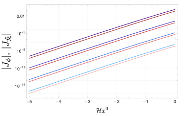
Figure 1: Absolute value of source terms $J_{\phi}$ (blue) and $J_{\tilde{\mathcal{R}}}$ (red) with $c=0.1$ for modes $k/M_{\mathrm{Pl}}\in\{10^{-3},\>10^{-2},\>10^{-1},\>10^{0}\}$ in the vicinity of the trans Planckian regime where darker colors correspond to larger modes. In the trans-Planckian regime $k/M_{\mathrm{Pl}}\sim 1$, $J_{\phi}$ and $J_{\tilde{\mathcal{R}}}$ become of order one at late times, while they remain small at all times in the sub-Planckian regime.

Comparing equations (27) and (29) with their classical GR counterparts (36) and (38), we notice that they in general contain an additional source term, $J_{\phi}$ and $J_{\tilde{\mathcal{R}}}$, respectively. The intrinsically quantum gravitational nature of these terms can be made manifest by solving first Eq. (24) under the requirement that solutions match the GR ones in the super-horizon limit. Indeed, in this case we can write

$$J_{\phi}=c\left(\frac{a^{2}k}{M_{\mathrm{Pl}}}\right)j_{\phi}[\bar{\phi}]\,,\qquad J_{\tilde{\mathcal{R}}}=c\left(\frac{a^{2}k}{M_{\mathrm{Pl}}}\right)j_{\tilde{\mathcal{R}}}[\bar{\phi}]\,,$$ (31)

where $c$ is the initial ratio of perturbed and background volume (and thus required to be small) and $j_{\phi}$ and $j_{\tilde{\mathcal{R}}}$ are functions depending on the background field $\bar{\phi}$ and the mode $k$. Visualized in Fig. 1, effects of the source terms remain small at all times in the sub-Planckian regime $k/M_{\mathrm{Pl}}\ll 1$ such that classical dynamics are recovered. Effects of the source terms become important in the trans-Planckian regime, $k/M_{\mathrm{Pl}}\gtrsim 1$, and therefore represent genuine quantum gravity effects.

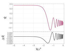
Figure 2: Top: Curvature-like perturbation $\tilde{\mathcal{R}}_{\mathrm{GFT}}$ (blue) and $\tilde{\mathcal{R}}_{\mathrm{GR}}$ (dashed red) for a fixed mode $k/M_{\mathrm{Pl}}=10^{2}$ in the trans-Planckian regime. Bottom: Difference of the blue and red dashed curves above, $\Delta\tilde{\mathcal{R}}\equiv\tilde{\mathcal{R}}_{\mathrm{GFT}}-\tilde{\mathcal{R}}_{\mathrm{GR}}$. For both plots, the ratio of $\delta V/\bar{V}$ and $\delta\phi$ at initial time has been set to $c=0.1$.

An exemplary solution of Eq. (29), together with a comparison to the classical GR counterpart is depicted in Fig. 2. As it is clear from the plots, QG corrections are only relevant for highly trans-Planckian modes, which are many orders of magnitude larger than the typical momentum scales of interest in cosmology ($\sim\text{Mpc}^{-1}$).

IV Conclusions

In this letter, we concretely realized the general expectation that non-trivial geometries emerge from quantum gravity entanglement Ryu and Takayanagi (2006); Bianchi and Myers (2014); Cao et al. (2017); Swingle (2018); Colafrancheschi (2022), by describing cosmological inhomogeneities in terms of relational nearest-neighbor two-body correlations between GFT quanta, encoded in entangled GFT coherent states. Our results therefore offer crucial insights into the potential intrinsically quantum gravitational nature of cosmological perturbations. More precisely, we show that these correlations produce macroscopic inhomogeneities in the expectation values of collective observables on the above states, such as the perturbed volume, $\delta V$, matter, $\delta\phi$, and the curvature-like perturbation $\tilde{\mathcal{R}}$. As the main result of this work, we extracted the dynamics of these cosmological perturbations from full QG (as described by the causally complete BC model), and showed that there are modifications with respect to the classical results. Crucially, these modifications, captured by the source terms $J_{\phi}$ and $J_{\tilde{\mathcal{R}}}$, are negligible on sub-Planckian scales and show relevance only in the trans-Planckian regime. Consequently, the modifications constitute genuine quantum effects arising from the microscopic spacetime structure. Although further work is needed to extend our analysis to: (i) non-isotropic and non-scalar perturbations, (ii) a more realistic matter content and (iii) to early relational times close to the quantum bounce Oriti et al. (2016, 2017); Marchetti and Oriti (2021a); Jercher et al. (2022a), this letter represents a substantial step towards constraining the underlying QG model with cosmological observations.

Finally, note that the extended causal structure of the complete BC model plays a crucial role in the derivation of the above results. Indeed, it is not only important for the construction of the entangled CPS, but it also allows for a consistent coupling of the physical Lorentzian reference frame, whose causal properties are a necessary ingredient to recover the classical dynamics in a low-energy limit. Seen in a broader context, these results strengthen the arguments for models that incorporate a causally complete set of discrete geometries such as CDT Loll (2020), causal sets Surya (2019) or Lorentzian spin foams Conrady and Hnybida (2010); Conrady (2010); Simão and Steinhaus (2021); Han et al. (2022a, b); Asante et al. (2021, 2022). Given the strong relations between GFT and these approaches, we hope that our results serve as an encouragement to employ a physical Lorentzian reference frame and to explore the relation between quantum geometric entanglement and cosmological perturbations in the latter.

Appendix A Appendix

A.1 Classical perturbation equations in harmonic gauge

The line element of scalar perturbations around a flat FLRW background in harmonic coordinates is given by

$$\differential{s}^{2}=-a^{6}(1+2A)\differential{t}^{2}+a^{4}\partial_{i}B\differential{t}\differential{x^{i}}+a^{2}\left((1-2\psi)\delta_{ij}+2\partial_{i}\partial_{j}E\right)\differential{x}^{i}\differential{x}^{j}.$$ (32)

Via the local spatial volume element, we identify the background and perturbed volume as

$$\bar{V}=a^{3},\qquad\frac{\delta V}{\bar{V}}=-3\psi+\nabla^{2}E.$$ (33)

Together with a minimally coupled massless scalar field $\phi=\bar{\phi}+\delta\phi$ with conjugate momentum $\pi_{\phi}$, background and perturbed equations of motion of the volume and the scalar field are given by

$$3\left(\frac{\bar{V}^{\prime}}{3\bar{V}}\right)^{2}=\frac{1}{2M_{\mathrm{Pl}}^{2}}\bar{\pi}_{\phi}^{2},$$ (34)

and

$$\left(\frac{\delta V}{\bar{V}}\right)^{\prime\prime}-a^{4}\nabla^{2}\left(\frac{\delta V}{\bar{V}}\right) =0,$$ (35)

$$\delta\phi^{\prime\prime}-a^{4}\nabla^{2}\delta\phi =0,$$ (36)

respectively.

To compare classical dynamics with that of GFT, we define the curvature-like perturbation $\tilde{\mathcal{R}}$

$$\tilde{\mathcal{R}}\equiv-\frac{\delta V}{3\bar{V}}+\mathcal{H}\frac{\delta\phi}{\bar{\phi}^{\prime}},$$ (37)

obeying

$$\tilde{\mathcal{R}}^{\prime\prime}-a^{4}\nabla^{2}\tilde{\mathcal{R}}=0.$$ (38)

Notice that in classical GR, $\tilde{\mathcal{R}}$ is explicitly gauge-dependent.

A.2 Source terms

Depicted in Fig. 1, the source terms entering the perturbed matter and curvature-like equations, (27) and (29), respectively, are given by

$$J_{\phi} =\left(-3\mathcal{H}\bar{\phi}+2\bar{\phi}^{\prime}\right)\left(\frac{\delta V}{\bar{V}}\right)^{\prime},$$ (39a)

$$J_{\tilde{\mathcal{R}}} =\left[3\mathcal{H}-\frac{1}{4M_{\mathrm{Pl}}^{2}}\left(\bar{\phi}^{2}\right)^{\prime}\right]\left(\frac{\delta V}{\bar{V}}\right)^{\prime}.$$ (39b)

For solutions of $\delta V/\bar{V}$ that match GR in the super-horizon limit, these terms explicitly evaluate to

$$J_{\phi}=-c\left(\frac{a^{2}k}{M_{\mathrm{Pl}}}\right)\bar{\phi}^{\prime}\left[-\frac{3}{\sqrt{6}}\bar{\phi}+2M_{\mathrm{Pl}}\right]\Gamma\left(\frac{7}{4}\right)$$

$$\quad\>\times\left(\frac{4\mathcal{H}}{a^{2}k}\right)^{3/4}J_{7/4}\left(\frac{a^{2}k}{2\mathcal{H}}\right)\,,$$ (40a)

$$J_{\tilde{\mathcal{R}}}=-c\left(\frac{a^{2}k}{M_{\mathrm{Pl}}}\right)\bar{\phi}^{\prime}\left[\frac{3}{\sqrt{6}}-\frac{\bar{\phi}}{2M_{\mathrm{Pl}}}\right]\Gamma\left(\frac{7}{4}\right)$$

$$\quad\>\times\left(\frac{4\mathcal{H}}{a^{2}k}\right)^{3/4}J_{7/4}\left(\frac{a^{2}k}{2\mathcal{H}}\right),$$ (40b)

where $c$ is an initial condition and $J_{\alpha}$ are Bessel functions of the first kind.

Alternatively, the source terms can be expressed in terms of conformal-longitudinal coordinates. In particular, $J_{\tilde{\mathcal{R}}}(\tau,k)$ is given by

$$J_{\tilde{\mathcal{R}}}(\tau,k)=\left[3H-\frac{1}{4M_{\mathrm{Pl}}^{2}}\derivative{\tau}\left(\bar{\phi}^{2}\right)\right]\derivative{\tau}\left(\frac{\delta V}{\bar{V}}\right),$$ (41)

which, upon solutions of $\delta V/\bar{V}$, is defined as

$$J_{\tilde{\mathcal{R}}}(\tau,k) =-c\left(\frac{k}{M_{\mathrm{Pl}}}\right)\derivative{\bar{\phi}}{\tau}\left[\frac{3}{\sqrt{6}}-\frac{\bar{\phi}}{2M_{\mathrm{Pl}}}\right]\Gamma\left(\frac{7}{4}\right)$$

$$\times\left(\frac{2}{k\tau}\right)^{3/4}J_{7/4}(k\tau).$$ (42)

References

- Blumenhagen et al. (2013) R. Blumenhagen, D. Lüst, and S. Theisen, Basic concepts of string theory, Theoretical and Mathematical Physics (Springer, Heidelberg, Germany, 2013).
- Percacci (2017) R. Percacci, An Introduction to Covariant Quantum Gravity and Asymptotic Safety (World Scientific, 2017) https://www.worldscientific.com/doi/pdf/10.1142/10369 .
- Reuter and Saueressig (2019) M. Reuter and F. Saueressig, Quantum Gravity and the Functional Renormalization Group: The Road towards Asymptotic Safety, Cambridge Monographs on Mathematical Physics (Cambridge University Press, 2019).
- Bonanno et al. (2020) A. Bonanno, A. Eichhorn, H. Gies, J. M. Pawlowski, R. Percacci, M. Reuter, F. Saueressig, and G. P. Vacca, Front. in Phys. 8, 269 (2020), arXiv:2004.06810 [gr-qc] .
- Ambjorn et al. (2012) J. Ambjorn, A. Goerlich, J. Jurkiewicz, and R. Loll, Phys. Rept. 519, 127 (2012), arXiv:1203.3591 [hep-th] .
- Hamber (2009) H. W. Hamber, Quantum Gravitation (Springer, Berlin, Heidelberg, 2009).
- Surya (2019) S. Surya, Living Rev. Rel. 22, 5 (2019), arXiv:1903.11544 [gr-qc] .
- Rovelli (2004) C. Rovelli, Quantum gravity, Cambridge Monographs on Mathematical Physics (Univ. Pr., Cambridge, UK, 2004).
- Rovelli (2011) C. Rovelli, PoS QGQGS2011, 003 (2011), arXiv:1102.3660 [gr-qc] .
- Perez (2013) A. Perez, Living Rev. Rel. 16, 3 (2013), arXiv:1205.2019 [gr-qc] .
- Asante et al. (2022) S. K. Asante, B. Dittrich, and S. Steinhaus, (2022), arXiv:2211.09578 [gr-qc] .
- Ashtekar and Lewandowski (2004) A. Ashtekar and J. Lewandowski, Class. Quant. Grav. 21, R53 (2004), arXiv:gr-qc/0404018 .
- Thiemann (2007) T. Thiemann, Modern Canonical Quantum General Relativity, Cambridge Monographs on Mathematical Physics (Cambridge University Press, 2007).
- Freidel (2005) L. Freidel, Int. J. Theor. Phys. 44, 1769 (2005), arXiv:hep-th/0505016 .
- Oriti (2011) D. Oriti, in Foundations of Space and Time: Reflections on Quantum Gravity (2011) pp. 257–320, arXiv:1110.5606 [hep-th] .
- Carrozza (2013) S. Carrozza, Tensorial methods and renormalization in Group Field Theories, Ph.D. thesis, Orsay, LPT (2013), arXiv:1310.3736 [hep-th] .
- Gurau (2016a) R. Gurau, SIGMA 12, 094 (2016a), arXiv:1609.06439 [hep-th] .
- Gurau (2016b) R. Gurau, Random Tensors (Oxford University Press, 2016).
- Aghanim et al. (2020) N. Aghanim et al. (Planck), Astron. Astrophys. 641, A6 (2020), [Erratum: Astron.Astrophys. 652, C4 (2021)], arXiv:1807.06209 [astro-ph.CO] .
- Oriti (2006) D. Oriti, , 310 (2006), arXiv:gr-qc/0607032 .
- Oriti (2016) D. Oriti, Class. Quant. Grav. 33, 085005 (2016), arXiv:1310.7786 [gr-qc] .
- Bonzom (2009) V. Bonzom, Phys. Rev. D 80, 064028 (2009), arXiv:0905.1501 [gr-qc] .
- Baratin and Oriti (2012) A. Baratin and D. Oriti, Phys. Rev. D 85, 044003 (2012), arXiv:1111.5842 [hep-th] .
- Baratin and Oriti (2011) A. Baratin and D. Oriti, New J. Phys. 13, 125011 (2011), arXiv:1108.1178 [gr-qc] .
- Loll (2020) R. Loll, Class. Quant. Grav. 37, 013002 (2020), arXiv:1905.08669 [hep-th] .
- Loll (1998) R. Loll, Living Rev. Rel. 1, 13 (1998), arXiv:gr-qc/9805049 .
- Gielen et al. (2013) S. Gielen, D. Oriti, and L. Sindoni, Phys. Rev. Lett. 111, 031301 (2013), arXiv:1303.3576 [gr-qc] .
- Gielen et al. (2014) S. Gielen, D. Oriti, and L. Sindoni, JHEP 06, 013 (2014), arXiv:1311.1238 [gr-qc] .
- Oriti et al. (2016) D. Oriti, L. Sindoni, and E. Wilson-Ewing, Class. Quant. Grav. 33, 224001 (2016), arXiv:1602.05881 [gr-qc] .
- Gielen and Sindoni (2016) S. Gielen and L. Sindoni, SIGMA 12, 082 (2016), arXiv:1602.08104 [gr-qc] .
- Pithis and Sakellariadou (2019) A. G. A. Pithis and M. Sakellariadou, Universe 5, 147 (2019), arXiv:1904.00598 [gr-qc] .
- Marchetti and Oriti (2021a) L. Marchetti and D. Oriti, JHEP 05, 025 (2021a), arXiv:2008.02774 [gr-qc] .
- Jercher et al. (2022a) A. F. Jercher, D. Oriti, and A. G. A. Pithis, JCAP 01, 050 (2022a), arXiv:2112.00091 [gr-qc] .
- Marchetti et al. (2023a) L. Marchetti, D. Oriti, A. G. A. Pithis, and J. Thürigen, JHEP 02, 074 (2023a), arXiv:2209.04297 [gr-qc] .
- Marchetti et al. (2023b) L. Marchetti, D. Oriti, A. G. A. Pithis, and J. Thürigen, Phys. Rev. Lett. 130, 141501 (2023b), arXiv:2211.12768 [gr-qc] .
- Marchetti and Oriti (2021b) L. Marchetti and D. Oriti, Front. Astron. Space Sci. 8, 683649 (2021b), arXiv:2010.09700 [gr-qc] .
- Marchetti and Oriti (2022) L. Marchetti and D. Oriti, JCAP 07, 004 (2022), arXiv:2112.12677 [gr-qc] .
- Gielen and Oriti (2018) S. Gielen and D. Oriti, Phys. Rev. D 98, 106019 (2018), arXiv:1709.01095 [gr-qc] .
- Gielen (2019) S. Gielen, JCAP 02, 013 (2019), arXiv:1811.10639 [gr-qc] .
- Gerhardt et al. (2018) F. Gerhardt, D. Oriti, and E. Wilson-Ewing, Phys. Rev. D 98, 066011 (2018), arXiv:1805.03099 [gr-qc] .
- Gielen and Mickel (2023) S. Gielen and L. Mickel, Universe 9, 29 (2023), arXiv:2211.04500 [gr-qc] .
- Jercher et al. (2022b) A. F. Jercher, D. Oriti, and A. G. A. Pithis, Phys. Rev. D 106, 066019 (2022b), arXiv:2206.15442 [gr-qc] .
- Barrett and Crane (2000) J. W. Barrett and L. Crane, Class. Quant. Grav. 17, 3101 (2000), arXiv:gr-qc/9904025 .
- Perez and Rovelli (2001a) A. Perez and C. Rovelli, Phys. Rev. D 64, 064002 (2001a), arXiv:gr-qc/0011037 .
- Perez and Rovelli (2001b) A. Perez and C. Rovelli, Phys. Rev. D 63, 041501 (2001b), arXiv:gr-qc/0009021 .
- Ryu and Takayanagi (2006) S. Ryu and T. Takayanagi, Phys. Rev. Lett. 96, 181602 (2006), arXiv:hep-th/0603001 .
- Bianchi and Myers (2014) E. Bianchi and R. C. Myers, Class. Quant. Grav. 31, 214002 (2014), arXiv:1212.5183 [hep-th] .
- Cao et al. (2017) C. Cao, S. M. Carroll, and S. Michalakis, Phys. Rev. D 95, 024031 (2017), arXiv:1606.08444 [hep-th] .
- Swingle (2018) B. Swingle, Annual Review of Condensed Matter Physics 9, 345 (2018).
- Colafrancheschi (2022) E. Colafrancheschi, Emergent spacetime properties from entanglement, Ph.D. thesis, University of Nottingham (2022).
- Li et al. (2017) Y. Li, D. Oriti, and M. Zhang, Class. Quant. Grav. 34, 195001 (2017), arXiv:1701.08719 [gr-qc] .
- (52) A. F. Jercher, R. Dekhil, and A. G. A. Pithis, work in progress .
- Jercher et al. (2023) A. F. Jercher, L. Marchetti, and A. G. A. Pithis, (2023), arXiv:2308.13261 [gr-qc] .
- Gielen (2016) S. Gielen, Class. Quant. Grav. 33, 224002 (2016), arXiv:1604.06023 [gr-qc] .
- Pithis and Sakellariadou (2017) A. G. A. Pithis and M. Sakellariadou, Phys. Rev. D 95, 064004 (2017), arXiv:1612.02456 [gr-qc] .
- Goeller et al. (2022) C. Goeller, P. A. Hoehn, and J. Kirklin, (2022), arXiv:2206.01193 [hep-th] .
- Gielen (2018) S. Gielen, Universe 4, 103 (2018), arXiv:1808.10469 [gr-qc] .
- de Cesare and Sakellariadou (2017) M. de Cesare and M. Sakellariadou, Phys. Lett. B 764, 49 (2017), arXiv:1603.01764 [gr-qc] .
- Perez and Sudarsky (2019) A. Perez and D. Sudarsky, Phys. Rev. Lett. 122, 221302 (2019), arXiv:1711.05183 [gr-qc] .
- Callen (1985) H. Callen, Thermodynamics and an Introduction to Thermostatistics (John Wiley & Sons, 1985).
- Lyth (1985) D. H. Lyth, Phys. Rev. D 31, 1792 (1985).
- Mukhanov (1988) V. F. Mukhanov, Sov. Phys. JETP 67, 1297 (1988).
- Mukhanov et al. (1992) V. Mukhanov, H. Feldman, and R. Brandenberger, Physics Reports 215, 203 (1992).
- Sasaki (1986) M. Sasaki, Progress of Theoretical Physics 76, 1036 (1986), https://academic.oup.com/ptp/article-pdf/76/5/1036/5152623/76-5-1036.pdf .
- Oriti et al. (2017) D. Oriti, L. Sindoni, and E. Wilson-Ewing, Class. Quant. Grav. 34, 04LT01 (2017), arXiv:1602.08271 [gr-qc] .
- Conrady and Hnybida (2010) F. Conrady and J. Hnybida, Class. Quant. Grav. 27, 185011 (2010), arXiv:1002.1959 [gr-qc] .
- Conrady (2010) F. Conrady, Class. Quant. Grav. 27, 155014 (2010), arXiv:1003.5652 [gr-qc] .
- Simão and Steinhaus (2021) J. D. Simão and S. Steinhaus, (2021), arXiv:2106.15635 [gr-qc] .
- Han et al. (2022a) M. Han, W. Kaminski, and H. Liu, Phys. Rev. D 105, 084034 (2022a), arXiv:2110.01091 [gr-qc] .
- Han et al. (2022b) M. Han, Z. Huang, H. Liu, and D. Qu, Phys. Rev. D 106, 044005 (2022b), arXiv:2110.10670 [gr-qc] .
- Asante et al. (2021) S. K. Asante, B. Dittrich, and J. Padua-Arguelles, Class. Quant. Grav. 38, 195002 (2021), arXiv:2104.00485 [gr-qc] .