Using Buckingham’s $\pi$ Theorem for Multi-System Learning Transfer:
a Case-study with 3 Vehicles Sharing a Database

Abstract

Learning schemes for planning and control are limited by the difficulty of collecting large amounts of experimental data or having to rely on high-fidelity simulations. This paper explores the potential of a proposed learning scheme that leverages dimensionless numbers based on Buckingham’s $\pi$ theorem to improve data efficiency and facilitate knowledge sharing between similar systems. A case study using car-like robots compares traditional and dimensionless learning models on simulated and experimental data to validate the benefits of the new dimensionless learning approach. Preliminary results show that this new dimensionless approach could accelerate the learning rate and improve the accuracy of the model and should be investigated further.

I Introduction

The typical approach to solving motion control problems for autonomous vehicles and other types of robotic systems is to use a physics-based kinematic or dynamic model of the system to plan trajectories and establish feedback laws [1][2][3]. With the rise of efficient machine learning algorithms, much effort has gone into using learning in planners and controllers so that autonomous vehicles can learn from experience and improve over time[4][5][6]. However, major difficulties limit the success of the learning scheme when it comes to controlling real physical platforms. One of the major challenges is the difficulty of collecting the large amount of experimental data required for advanced learning schemes such as deep-learning [6][7]. A popular solution is to generate data using high-fidelity simulations instead of experiments. Nevertheless, this approach also has multiple challenges, such as the difficulty of capturing certain behaviors in a simulator and transferring the results to the real world [8]. All in all, data efficiency is a critical bottleneck.

Sharing learned data and policies across multiple systems could help solve the problem of collecting huge amounts of data. For example, instead of having to start learning from scratch, a centralized database for a fleet of vehicles would enable the newly deployed vehicle to use knowledge based on thousands of hours of motion data collected by hundreds of vehicles. However, this is difficult to achieve when the studied systems do not share identical characteristics as their behavior, and therefore the appropriate control policy, differs. This paper investigates the potential of leveraging dimentionless number and the Buckingham’s $\pi$ theorem to help learning more general models. Section II presents some related work and discusses the original contribution of this paper. Section III defines the problem used as the case study in this paper. Section IV presents the learning results based on simulated data and section V presents the learning results based on an experimental validation with three small scale vehicles shown at Fig. 1 .

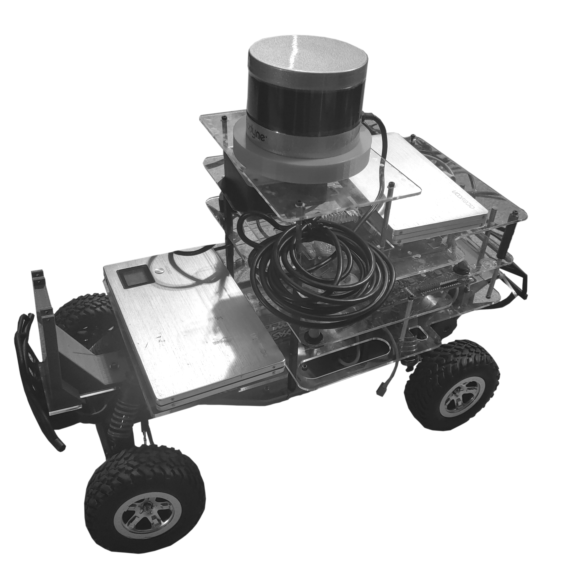
(a) Small vehicle

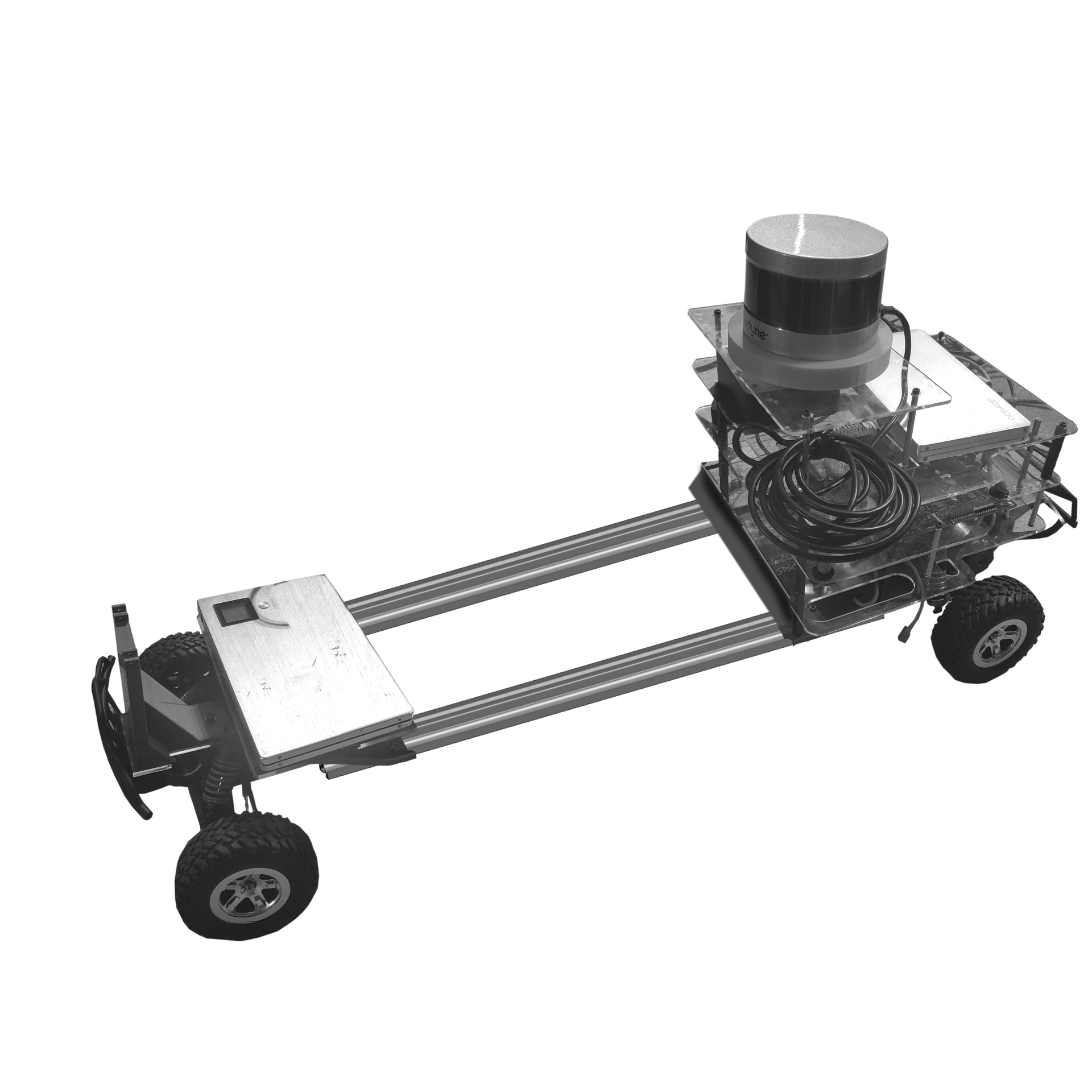
(b) Long vehicle

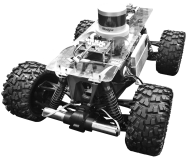
(c) Large vehicle

Figure 1: Small scale platforms of various dimensions used for experimental validation.

II Background

Multi-task transfer learning has received significant research attention recently [9][10][11]. This paper focuses on multi-system transfer where the objective is to share knowledge between similar systems that accomplish the same task. Specifically for multi-system transfer, an interesting approach is presented in [12] where a shared database can outperform a robot-specific training approach that uses 4x-20x more data. In [13], the authors address the problem of inappropriate transfer, which can result in a decrease in performance. By assessing how similar two systems are, it is possible to know with which systems the transfer learning would be most beneficial. The closest related work is probably [14], where the authors rather tackle the problem directly by guiding the policies network with a representation vector built from information regarding the hardware. This approach is similar to the one presented in this work, but instead of two vectors, one containing the states and the other containing the characteristics of the hardware, a single vector is built based on these features with the intention of reducing the dimensions of the system to zero by using the Buckingham’s $\pi$ theorem.

Dimensional analysis [15], i.e. the Buckingham’s $\pi$ theorem, is a useful tool to simplify input/output relationships that involved physical quantities. It is used extensively in the field of fluid mechanics to minimize the number of experiments required to characterize a behaviour. Also, there is a renew interest in using dimensional analysis in the context of learning [16] [17] [18]. However, dimensional analysis it still very seldomly explored in the field of motion control and robotics, to our knowledge only a few projects used that concept. In the case of an in-lane collision avoidance system, [19] created dimensionless indices, based on a vehicle’s relative longitudinal velocity, road surface conditions and terminal lateral distance, which were used in the selection of the most efficient maneuver and timing for an intervention. The use of these indices was shown to be computationally efficient. The authors of [20] proposed an improved method for kinematic calibration based on dimensionless error mapping matrices (EMMs). Simulation results show that the residual pose errors with the proposed dimensionless EMMs were lower than with the conventional EMM in various units. Finally, [21] discuss the notion that similar dynamic systems must have an equivalent optimal policy when expressed in dimensionless form.

Here in this paper, the novelty is to leverage dimensional analysis to improve data efficiency for learning motion models of similar vehicles. The contributions are: 1) A new way to describe a system using an Augmented Buckingham’s $\pi$ theorem based model is presented. 2) A demonstration of how that dimensionless model can be a way to generalize learning in the context of motion control by being able to share knowledge with different systems is made. 3) A case study with robotic vehicles is used to show through simulations and experiments that this dimensionless learning scheme is advantageous compared to baseline approaches.

III Problem definition for the case-study

The main goal of this paper is to validate whether a learning scheme can benefit from a dimensionless mapping of its inputs and outputs. These benefits could take the form of an increase in learning speed, a reduction in mean absolute error (MAE) and the possibility of sharing knowledge between similar systems. To do so, different optimized distributed gradient boosting (XGBoost) models have been trained with simulated and experimental data and compared using their respective MAE. Two dimensionless learning schemes have been created and compared with a baseline traditional dimensional model. The first one is based on applying the Buckingham’s $\pi$ theorem to the input/output relationship that is modeled. The second, called the Augmented Buckingham’s $\pi$ theorem based model, is also based on the Buckingham’s $\pi$ theorem but with additionnal dimensionless inputs (hand crafted features based on expert knowledge of the system’s physics).

Inspired by the challenges of learning good control policies for emergency braking maneuvers on various ground conditions (snow, ice, etc.), such as explored in [22], the presented case study is the prediction of the final relative position of a vehicle after a sudden emergency maneuver, based on initial conditions, control inputs (braking and steering), and environmental parameters. The learned model could be then used in a control pipeline to select the best maneuver in an emergency braking situation for instance. To simplify the case study a few assumptions are made. Firstly, the control inputs are constant throughout a maneuver, i.e. the steering angle $\delta$ and braking action (constant deceleration rate $a$ imposed on both rear wheels) are decided once at the start of the maneuver and remain constant until the vehicle comes to a complete stop. Also, only the final position of the vehicle is predicted, not the complete trajectory. Furthermore, the environment is always a horizontal surface and only 2D planar motion is taken into account. The simulation only consider a kinematic motion model, while for the experimental data the dynamics of the system is taken into account, neglecting any roll or pitch effects and considering the complex soil-tire relationship simply as a constant coefficient of friction $\mu$. Table I shows the main variables involved in this case study.

TABLE I: Variables used throughout this paper

Variables	Descriptions	Units [Dimensions]
State variables
$X$	Position of the vehicle in X-axis of world frame	m [L]
$Y$	Position of the vehicle in Y-axis of world frame	m [L]
$\theta$	Yaw of the vehicle in world frame	rad
Environment related variables
$\mu$	Friction coefficient wheels/road	-
$v$	Longitudinal velocity of the vehicle	m/s [LT-1]
$g$	Gravitational acceleration	m/s2 [LT-2]
maneuvers related variables
$a$	Deceleration of the wheel	m/s2 [LT-2]
$\delta$	Steering angle of front wheels	rad
Vehicles related variables
$N_{f}$	Normal force on front wheels	N [MLT-2]
$N_{r}$	Normal force on rear wheels	N [MLT-2]
$l$	Length between vehicle’s axles	m [L]

Three small scale car-like vehicles of various dimension are used for both validation processes (simulation and experimentation). Vehicle 1, shown in figure 1a, is a modified 1:10 scale platform based on a Traxxas SLASH. The vehicle 2, shown in figure 1b, is also a modified 1:10 scale platform based on a Traxxas SLASH with the chassis modified to have a longer wheelbase. Finally, vehicle 3, shown in figure 1c, is a modified 1:5 scale platform based on a Traxxas X-MAXX. From now on, they will be referred to as small vehicle, long vehicle and large vehicle respectively. Their specifications are summarized in table II. Since the simulation only takes kinematics into account, only the wheelbase length l of these vehicles is used to describe them in that particular section.

TABLE II: Specifications of all vehicles

Vehicle	$l$	$N_{f}$	$N_{r}$
	(m)	(N)	(N)
Small	0.345	37.77	28.84
Long	0.853	22.74	52.89
Large	0.475	71.12	71.12

IV Learning with simulated data

IV-A Simulator presentation

This section presents an analysis in which the proposed learning approach is evaluated using data generated in a simplified simulated environment. The simulation was based on the kinematic bicycle model frequently used in the literature. The non-linear equations for the bicycle model are shown at 1.

$$\begin{bmatrix}\dot{X}\\ \dot{Y}\\ \dot{\theta}\\ \dot{v}\\ \end{bmatrix}=\begin{bmatrix}vcos(\theta)\\ vsin(\theta)\\ \frac{vtan(\delta)}{l}\\ a\\ \end{bmatrix}$$ (1)

For all three vehicles presented at figure 1, 5 500 simulations were conducted with the initial values and maneuvers shown at table III

TABLE III: Values for the simulations for all 3 vehicles

$v_{i}$	$a$	$\delta$
(m/s)	(m/s2)	(rad)
From 0.1	From -0.1 g	From 0.0000
to 5.0	to -1.0 g	to 0.7854
by 0.1	by -0.1 g	by 0.0785
50 values	10 values	11 values

All simulations start with the vehicle at position [X,Y] = (0,0), orientation $\theta$ = 0 rad and initial speed $v_{i}$. The maneuver starts right away with deceleration $a$ and steering angle $\delta$. The simulation stops when the vehicle reach zero velocity and the final position and orientation are noted.

IV-B Learning model types for the simulation

IV-B1 Traditional dimensionalized learning model

The nonlinear equations describing the kinematic bicycle model used for the simulation presented at 1 can be written in the form of 2.

$$\begin{bmatrix}X,Y,\theta\end{bmatrix}=f(v_{i},a,\delta,l)$$ (2)

Thus, the dimensionalized parameters for the initial velocity $v_{i}$, the decelaration a, the steering angle $\delta$ and the length of the wheelbase l are used as inputs to the XGBoost algorithm to predict the final pose [X,Y,$\theta$] of the vehicle. This traditional dimensionalized learning scheme is illustrated at figure 2

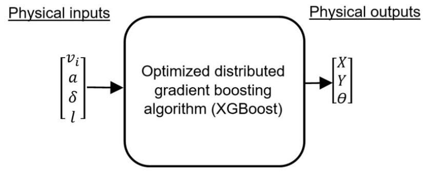
Figure 2: Baseline learning scheme for simulated data

IV-B2 Buckingham’s $\pi$ theorem based model

According to Buckingham’s $\pi$ theorem, with N dimensionalized variables and P independent dimensions, we obtain m = N - P dimensionless numbers. Here, N = 7 [$X$, $Y$, $\theta$, $v_{i}$, $a$, $\delta$, $l$] and P = 2 [L,T]. We thus have five dimensionless numbers. By using the distance between the two axles $l$ [M] and the initial velocity of the vehicle $v_{i}$ [MT^-1] as repeated variables, we can create the five dimensionless numbers. The inputs and ouputs of the XGBoost algorithm used to predict the outcome of a maneuver are shown on figure 3.

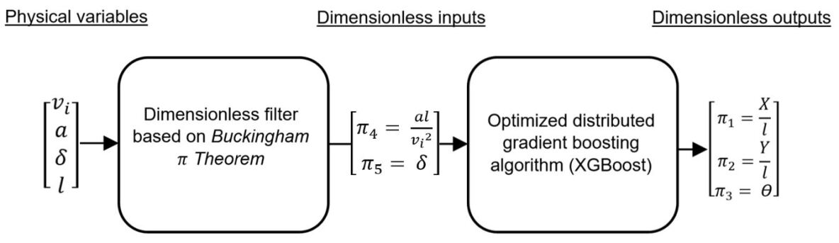
Figure 3: Buckingham’s $\pi$ theorem based model for simulated data

IV-B3 Augmented Buckingham’s $\pi$ theorem based model

Based on the mathematical shape of the nonlinear equation for $\dot{\theta}$ presented at equation 1, we obtain the arbitrary dimensionless number $\pi_{6}$ derived at 3. The inputs and ouputs of the Augmented Buckingham’s $\pi$ theorem based model used to predict the outcome of a maneuver are shown on figure 4.

$$\dot{\theta}=\frac{vtan(\delta)}{l}\hskip 2.84544pt;\hskip 14.22636pt\pi_{6}=\frac{{v^{2}}tan(\delta)}{al}$$ (3)

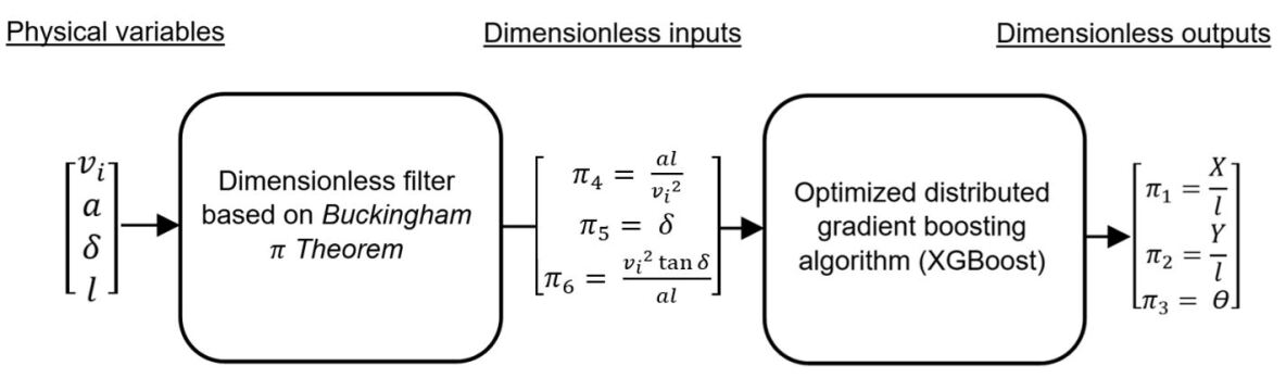
Figure 4: Augmented Buckingham’s $\pi$ theorem based model for simulated data

IV-C Results

The results for the three model types will be examined from two perspectives. On the one hand, we will study the MAEs of self-predictions, cross-predictions and shared-predictions for each model type. On the other hand, we will examine the effect of the size of the training set on the convergence of the MAEs for self-predictions, or the so-called the learning rate of the models.

IV-C1 Mean absolute error

The MAE is one of the most widely used metrics for regression algorithms since it has the same units as the model’s dependent variables which makes the results easier to understand. Equation 4 shows how MAE is calculated, where N is the number of tests used, $y_{i}$ are the actual result values and $\hat{y}_{i}$ are the predicted values. Since the output values for both dimensionless models are $\pi_{1}$ = $\frac{X}{l}$, $\pi_{2}$ = $\frac{Y}{l}$ and $\pi_{3}$ = $\theta$, $\pi_{1}$ and $\pi_{2}$ are multiplied by the wheelbase $l$ of the tested vehicle before computing the MAE so that all resultats share the same units.

$$MAE=\frac{1}{N}\sum_{i=1}^{N}|(y_{i}-\hat{y}_{i})|$$ (4)

80$\%$ of the simulated data were used to train a model of each type for the three vehicles. The remaining 20$\%$ is used to test the models. Table IV contains the results of the traditional dimensionalized model, the results of the model based on Buckingham’s $\pi$ theorem are presented in table V and table VI shows the results of the Augmented Buckingham model. For all three tables, the light gray cells correspond to the results of what we call self-predictions, i.e. predictions that use a vehicle’s test set in its own trained model. The white cells correspond to the results of a vehicle’s test set in another vehicle’s trained model, known as cross-predictions. Finally, the dark gray cells are the results of shared predictions. For shared predictions, the test set of a particular vehicle is ran in a model that has been trained with data from all three vehicles.

TABLE IV: MAEs for the traditional dimensionalized model (X and Y are in meters and $\theta$ in rad)

Models	Data Vehicle 1	Data Vehicle 2	Data Vehicle 3
	(Small)	(Long)	(Large)
Model	X: 0.0494	X: 0.3703	X: 0.1601
Vehicle 1	Y: 0.0466	Y: 0.3071	Y: 0.1459
(Small)	$\theta$: 0.0587	$\theta$: 0.9851	$\theta$: 0.4502
Model	X: 0.3653	X: 0.0316	X: 0.2622
Vehicle 2	Y: 0.3032	Y: 0.0257	Y: 0.2061
(Long)	$\theta$: 0.9919	$\theta$: 0.0238	$\theta$: 0.5369
Model	X: 0.1667	X: 0.2679	X: 0.0414
Vehicle 3	Y: 0.1440	Y: 0.2125	Y: 0.0362
(Large)	$\theta$: 0.4599	$\theta$: 0.5324	$\theta$: 0.0422
Model	X: 0.0467	X: 0.0433	X: 0.0514
MERGED	Y: 0.0465	Y: 0.0368	Y: 0.0498
(All 3)	$\theta$: 0.0457	$\theta$: 0.0302	$\theta$: 0.0431

TABLE V: MAEs for the Buckingham’s $\pi$ theorem based model (X and Y are in meters and $\theta$ in rad)

Models	Data Vehicle 1	Data Vehicle 2	Data Vehicle 3
	(Small)	(Long)	(Large)
Model	X: 0.0204	X: 0.0144	X: 0.0125
Vehicle 1	Y: 0.0261	Y: 0.0102	Y: 0.0099
(Small)	$\theta$: 0.0331	$\theta$: 0.0109	$\theta$: 0.0159
Model	X: 0.0354	X: 0.0145	X: 0.0303
Vehicle 2	Y: 0.0394	Y: 0.0176	Y: 0.0262
(Long)	$\theta$: 0.2007	$\theta$: 0.0127	$\theta$: 0.0917
Model	X: 0.0153	X: 0.0103	X: 0.0190
Vehicle 3	Y: 0.0162	Y: 0.0095	Y: 0.0182
(Large)	$\theta$: 0.0666	$\theta$: 0.0097	$\theta$: 0.0241
Model	X: 0.0080	X: 0.0087	X: 0.0083
MERGED	Y: 0.0086	Y: 0.0087	Y: 0.0083
(All 3)	$\theta$: 0.0143	$\theta$: 0.0080	$\theta$: 0.0115

TABLE VI: MAEs for the Augmented Buckingham’s $\pi$ theorem based model (X and Y are in meters and $\theta$ in rad)

Models	Data Vehicle 1	Data Vehicle 2	Data Vehicle 3
	(Small)	(Long)	(Large)
Model	X: 0.0126	X: 0.0117	X: 0.0104
Vehicle 1	Y: 0.0121	Y: 0.0090	Y: 0.0077
(Small)	$\theta$: 0.0131	$\theta$: 0.0043	$\theta$: 0.0063
Model	X: 0.0271	X: 0.0103	X: 0.0219
Vehicle 2	Y: 0.0286	Y: 0.0134	Y: 0.0222
(Long)	$\theta$: 0.1407	$\theta$: 0.0052	$\theta$: 0.0591
Model	X: 0.0130	X: 0.0090	X: 0.0117
Vehicle 3	Y: 0.0133	Y: 0.0091	Y: 0.0129
(Large)	$\theta$: 0.0389	$\theta$: 0.0038	$\theta$: 0.0098
Model	X: 0.0045	X: 0.0055	X: 0.0046
MERGED	Y: 0.0050	Y: 0.0061	Y: 0.0051
(All 3)	$\theta$: 0.0060	$\theta$: 0.0028	$\theta$: 0.0035

Table VII summarizes the three previous tables (IV, V and VI). For self-predictions, we can see that the Buckingham’s $\pi$ theorem based model and the Augmented Buckingham model are respectively 1.93 times and 3.60 times more precise than the traditional model. These numbers climb to 11.76 times and 15.80 times for cross-predictions. Finaly, the Buckingham’s $\pi$ theorem based model and the Augmented Buckingham model are respectively 4.80 times and 9.17 times more precise than the traditional model in shared-predictions.

TABLE VII: MAEs comparison for all models trained with simulated data (X and Y are in meters and $\theta$ in rad)

Prediction	Traditional	Buckingham’s	Augmented
types	dimensionalized	$\pi$ theorem	Buckingham’s
	model	based model	$\pi$ model
SELF	X: 0.0408	X: 0.0180	X: 0.0115
Predictions	Y: 0.0362	Y: 0.0206	Y: 0.0128
	$\theta$: 0.0416	$\theta$: 0.0233	$\theta$: 0.0094
CROSS	X: 0.2654	X: 0.0197	X: 0.0155
Predictions	Y: 0.2198	Y: 0.0186	Y: 0.0128
	$\theta$: 0.6594	$\theta$: 0.0659	$\theta$: 0.0422
SHARED	X: 0.0471	X: 0.0083	X: 0.0049
Predictions	Y: 0.0444	Y: 0.0085	Y: 0.0054
	$\theta$: 0.0397	$\theta$: 0.0113	$\theta$: 0.0041

IV-C2 Learning rate

The amount of data required to obtain an operational predictive function for self-predictions for all model types is then investigated. Figure 5 shows the MAE convergence for the final longitudinal position $X$, final lateral position $Y$ and final yaw $\theta$ of the three model types with the large vehicle’s self-predictions. For all outputs, the Augmented Buckingham model converges the fastest, followed by the Buckingham’s $\pi$ theorem based model. More data would be required to achieve full convergence of the final $X$ and $Y$ positions for the traditional dimensionalized model. Only the data for the large vehicle is presented to avoid any redundancy since all curves were alike.

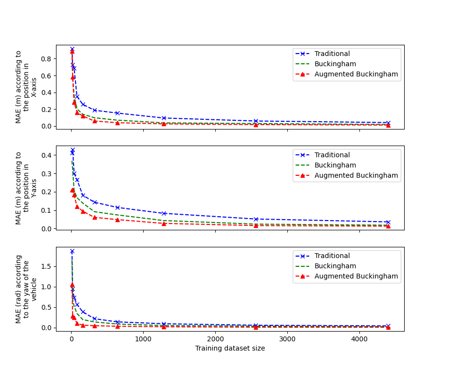
Figure 5: MAE convergence according to training size for the simulated data of the large vehicle

V Learning with experimental data

V-A Tests used for generating the data

For all three vehicles, 540 experimental tests were carried out with the initial values and maneuvers shown in table VIII. All tests start with the vehicle in position (0,0), orientation 0 rad, initial speed $v_{i}$ and ground/tire friction coefficient $\mu$. The maneuver begins immediately with deceleration $a$ and steering angle $\delta$. The test stops when the vehicle has come to a complete stop, and the final position and orientation are recorded using a VICON triangulation camera system.

TABLE VIII: Values for the experimental tests for all 3 vehicles

$\mu$	$v_{i}$	$a$	$\delta$
	(m/s)	g (9.81 m/s2)	(rad)
0.2	From 1.0	From 0.1	0.0000
0.4	to 3.5	to 1.0	0.3927
0.9	by 0.5	by 0.1	0.7854
3 values	6 values	10 values	3 values

V-B Learning model types for the experimental validation

V-B1 Traditional dimensionnalized learning model

With the assumptions made in section III and based on table I, the equation 5 can be written for the experimental end position [$X$,$Y$,$\theta$]. The baseline learning scheme for the experimental validation is illustrated at figure 6.

$$\begin{bmatrix}X,Y,\theta\end{bmatrix}=f(\mu,v_{i},g,a,\delta,N_{f},N_{r},l)$$ (5)

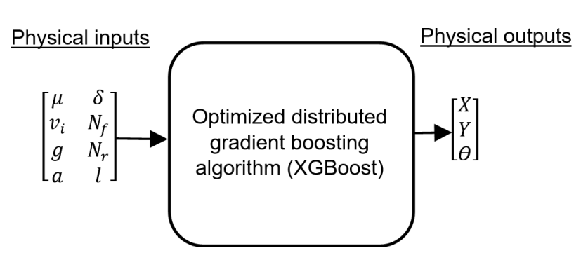
Figure 6: Baseline learning scheme for experimental data

V-B2 Buckingham $\pi$ theorem based model

According to Buckingham $\pi$ theorem, N = 11 [$\mu$, $v_{i}$, $g$, $a$, $\delta$, $N_{f}$, $N_{r}$ , $l$, $X$, $Y$, $\theta$] and P = 3 [M,L,T]. We thus have eight dimensionless numbers. By using the distance between the two axles $l$ [M], the initial velocity of the vehicle $v_{i}$ [MT^-1] and the normal force on front wheels $N_{f}$ [MLT^-2] as repeated variables, we get the eight dimensionless numbers. The inputs and ouputs of the XGBoost algorithm are used to predict the outcome of a maneuver are shown on figure 7.

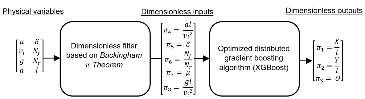
Figure 7: Buckingham’s $\pi$ theorem based model for experimental data

V-B3 Augmented Buckingham $\pi$ theorem based model for experimental data

By simple manipulations of the same physical variables used in previous models, the limits in longitudinal force $\pi_{9}$ and lateral force $\pi_{10}$ before sliding can be introduced using equations 6 and 7. An infinite number of corrective dimensionless numbers could be created depending on the system under study to minimize the output error of the Augmented Buckingham model. However, these two numbers have been arbitrarily chosen for their high dynamic significance.

$$\pi_{9}=\frac{F_{limit}}{F_{x_{maneuver}}}=\frac{N_{r}\mu}{ma}=\frac{N_{r}\mu g}{(N_{f}+N_{r})a}$$ (6)

$$\pi_{10}=\frac{F_{limit}}{F_{y_{maneuver}}}=\frac{N_{r}\mu}{\frac{mv^{2}}{R}}=\frac{g\mu R}{v^{2}}=\frac{g\mu l}{v^{2}\tan\delta}$$ (7)

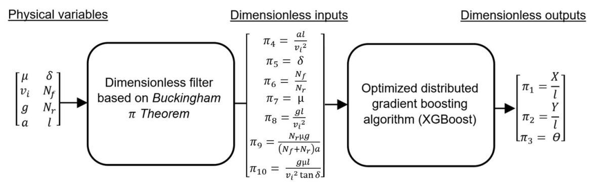
Figure 8: Augmented Buckingham’s $\pi$ theorem based model for experimental data

V-C Results

V-C1 Mean Absolute Error

To avoid any redudancy, only the summarizing table IX for self, cross and shared-predictions is presented for the experimental data. For self-predictions, we can see that the Buckingham’s $\pi$ theorem based model and the Augmented Buckingham model are respectively 1.11 times and 1.14 times more precise than the traditional model on average. These numbers drop to 1.05 times and 1.07 times more precise for cross-predictions. Finaly, the Buckingham’s $\pi$ theorem based model and the Augmented Buckingham model are respectively 1.11 times and 1.28 times more precise than the traditional model in shared-predictions.

TABLE IX: MAE comparison for all models trained with experimental data (X and Y are in meters and $\theta$ in rad)

Prediction	Traditional	Buckingham’s	Augmented
types	dimensionalized	$\pi$ theorem	Buckingham’s
	model	based model	$\pi$ model
SELF	X: 0.1229	X: 0.1228	X: 0.1197
Predictions	Y: 0.0488	Y: 0.0321	Y: 0.0335
	$\theta$: 0.0482	$\theta$: 0.0596	$\theta$: 0.0554
CROSS	X: 0.3027	X: 0.3752	X: 0.3775
Predictions	Y: 0.2198	Y: 0.0186	Y: 0.0128
	$\theta$: 0.2007	$\theta$: 0.1494	$\theta$: 0.1454
SHARED	X: 0.0539	X: 0.0507	X: 0.0400
Predictions	Y: 0.0130	Y: 0.0105	Y: 0.0089
	$\theta$: 0.0193	$\theta$: 0.0187	$\theta$: 0.0187

V-C2 Learning rate

Figure 9 shows the MAE convergence for the final longitudinal position $X$, final lateral position $Y$ and final yaw $\theta$ of the three model types with the large vehicle’s experimental self-predictions. For all outputs, all three models follow a similar learning curve. More training data (limited here by the number of experimental test conducted) would be required to fully converge since all curves keep on improving at a relatively high rate.

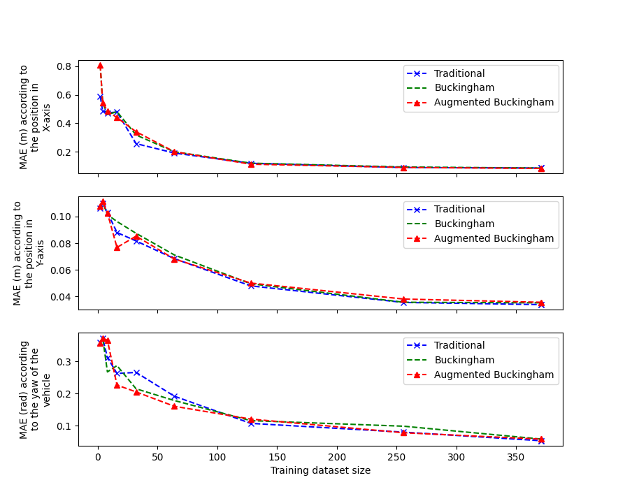
Figure 9: MAE convergence according to training size for the experimental data of the large vehicle

VI Conclusion

To conclude, this paper presents a new dimensionless learning scheme based on Bucking’s $\pi$ theorem. The results with data based on kinematic simulations show that the proposed dimensionless models are much more accurate when using a shared database, and have faster learning rates than a traditional dimensional model. The experimental validation also shown some advantage with the proposed dimensionless scheme over a baseline approach in a complex dynamical context, but the gain was less significant ($\approx$10% compared to 10x for the kinematic behavior in simulation), probably due to a discrepancy between the assumptions made (i.e. when selecting the list of input variables for the dimensional analysis) and the high complexity of the tire dynamics involved in the experiments. All in all, the early results presented in this case-study show that leveraging Bucking’s $\pi$ theorem can minimize the experimental data required to train a learning algorithm modelling a physical phenomena. Hence, this novel approach should be investigated further to better understand its full potential and limitation.

References

- [1] N. H. Amer, H. Zamzuri, K. Hudha, and Z. A. Kadir, “Modelling and control strategies in path tracking control for autonomous ground vehicles: A review of state of the art and challenges,” vol. 86, no. 2, pp. 225–254. [Online]. Available: http://link.springer.com/10.1007/s10846-016-0442-0
- [2] B. Paden, M. Čáp, S. Z. Yong, D. Yershov, and E. Frazzoli, “A Survey of Motion Planning and Control Techniques for Self-Driving Urban Vehicles,” IEEE Transactions on Intelligent Vehicles, vol. 1, no. 1, pp. 33–55, Mar. 2016.
- [3] C. Katrakazas, M. Quddus, W.-H. Chen, and L. Deka, “Real-time motion planning methods for autonomous on-road driving: State-of-the-art and future research directions,” vol. 60, pp. 416–442. [Online]. Available: https://linkinghub.elsevier.com/retrieve/pii/S0968090X15003447
- [4] S. Aradi, “Survey of deep reinforcement learning for motion planning of autonomous vehicles,” vol. 23, no. 2, pp. 740–759, conference Name: IEEE Transactions on Intelligent Transportation Systems.
- [5] R. H. Crites and A. G. Barto, “Improving elevator performance using reinforcement learning,” p. 7.
- [6] X. Di and R. Shi, “A survey on autonomous vehicle control in the era of mixed-autonomy: From physics-based to AI-guided driving policy learning,” vol. 125, p. 103008. [Online]. Available: https://linkinghub.elsevier.com/retrieve/pii/S0968090X21000401
- [7] B. M. Lake, T. D. Ullman, J. B. Tenenbaum, and S. J. Gershman, “Building machines that learn and think like people,” vol. 40, publisher: Cambridge University Press. [Online]. Available: http://www.cambridge.org/core/journals/behavioral-and-brain-sciences/article/building-machines-that-learn-and-think-like-people/A9535B1D745A0377E16C590E14B94993
- [8] Y. Liu, H. Xu, D. Liu, and L. Wang, “A digital twin-based sim-to-real transfer for deep reinforcement learning-enabled industrial robot grasping,” vol. 78, p. 102365. [Online]. Available: https://linkinghub.elsevier.com/retrieve/pii/S0736584522000539
- [9] S. Dey, S. Boughorbel, and A. F. Schilling, “Learning a shared model for motorized prosthetic joints to predict ankle-joint motion.” [Online]. Available: http://arxiv.org/abs/2111.07419
- [10] O. M. Andrychowicz, B. Baker, M. Chociej, R. Józefowicz, B. McGrew, J. Pachocki, A. Petron, M. Plappert, G. Powell, A. Ray, J. Schneider, S. Sidor, J. Tobin, P. Welinder, L. Weng, and W. Zaremba, “Learning dexterous in-hand manipulation,” vol. 39, no. 1, pp. 3–20, publisher: SAGE Publications Ltd STM. [Online]. Available: https://doi.org/10.1177/0278364919887447
- [11] A. Nagabandi, I. Clavera, S. Liu, R. S. Fearing, P. Abbeel, S. Levine, and C. Finn, “Learning to adapt in dynamic, real-world environments through meta-reinforcement learning.” [Online]. Available: http://arxiv.org/abs/1803.11347
- [12] S. Dasari, F. Ebert, S. Tian, S. Nair, B. Bucher, K. Schmeckpeper, S. Singh, S. Levine, and C. Finn, “RoboNet: Large-scale multi-robot learning.” [Online]. Available: http://arxiv.org/abs/1910.11215
- [13] M. J. Sorocky, S. Zhou, and A. P. Schoellig, “Experience selection using dynamics similarity for efficient multi-source transfer learning between robots.” [Online]. Available: http://arxiv.org/abs/2003.13150
- [14] T. Chen, A. Murali, and A. Gupta, “Hardware conditioned policies for multi-robot transfer learning,” in Advances in Neural Information Processing Systems, vol. 31. Curran Associates, Inc. [Online]. Available: https://proceedings.neurips.cc/paper/2018/hash/b8cfbf77a3d250a4523ba67a65a7d031-Abstract.html
- [15] M. E. Buckingham, “On Physically Similar Systems; Illustrations of the Use of Dimensional Equations,” Physical Review, Oct. 1914, publisher: American Physical Society (APS). [Online]. Available: https://www.scienceopen.com/document?vid=805fe995-1849-413a-b228-3fe616732290
- [16] J. Bakarji, J. Callaham, S. L. Brunton, and J. N. Kutz, “Dimensionally consistent learning with Buckingham Pi,” Nature Computational Science, vol. 2, no. 12, pp. 834–844, Dec. 2022. [Online]. Available: https://www.nature.com/articles/s43588-022-00355-5
- [17] K. Fukami and K. Taira, “Robust machine learning of turbulence through generalized Buckingham Pi-inspired pre-processing of training data,” p. A31.004, Jan. 2021, conference Name: APS Division of Fluid Dynamics Meeting Abstracts ADS Bibcode: 2021APS..DFDA31004F. [Online]. Available: https://ui.adsabs.harvard.edu/abs/2021APS..DFDA31004F
- [18] X. Xie, A. Samaei, J. Guo, W. K. Liu, and Z. Gan, “Data-driven discovery of dimensionless numbers and governing laws from scarce measurements,” Nature Communications, vol. 13, no. 1, p. 7562, Dec. 2022, number: 1 Publisher: Nature Publishing Group. [Online]. Available: https://www.nature.com/articles/s41467-022-35084-w
- [19] A. S. P. Singh and N. Osamu, “Nondimensionalized indices for collision avoidance based on optimal control theory,” in 36th FISITA World Automotive Congress, 2016, September 26, 2016 - September 30, 2016, ser. FISITA 2016 World Automotive Congress - Proceedings. FISITA.
- [20] X. Luo, F. Xie, X.-J. Liu, and Z. Xie, “Kinematic calibration of a 5-axis parallel machining robot based on dimensionless error mapping matrix,” vol. 70, p. 102115. [Online]. Available: https://linkinghub.elsevier.com/retrieve/pii/S0736584521000016
- [21] A. Girard, “Dimensionless policies based on the buckingham theorem: Is it a good way to generalize numerical results?” 2023.
- [22] O. Lecompte, W. Therrien, and A. Girard, “Experimental investigation of a maneuver selection algorithm for vehicles in low adhesion conditions,” vol. 7, no. 3, pp. 407–412, conference Name: IEEE Transactions on Intelligent Vehicles.