Exact lattice chiral symmetry in 2d gauge theory

Abstract

We construct symmetry-preserving lattice regularizations of 2d QED with one and two flavors of Dirac fermions, as well as the ‘$3450$’ chiral gauge theory, by leveraging bosonization and recently-proposed modifications of Villain-type lattice actions. The internal global symmetries act just as locally on the lattice as they do in the continuum, the anomalies are reproduced at finite lattice spacing, and in each case we find a sign-problem-free dual formulation.

Introduction. Numerical Monte Carlo simulations of quantum field theories (QFTs) discretized on Euclidean spacetime lattices are one of the few known non-perturbative techniques to study strongly coupled QFTs. However, it is famously difficult to discretize fermions while preserving all of their symmetries Kaplan (2009). For example, a free massless Dirac fermion has the internal global symmetry $\left[(U(1)_{V}\times U(1)_{A})/\mathbb{Z}_{2}\right]\rtimes(\mathbb{Z}_{2})_{C}$ for even $d$. The continuous symmetries have a mixed ’t Hooft anomaly, and standard lattice regularizations do not preserve the continuum version of the chiral symmetry at finite lattice spacing $a$.

If we integrate out a massless Dirac fermion in a Euclidean QFT, we obtain the path integral

$$Z=\int\mathcal{D}\phi\det\left[\not{D}(\phi)\right]e^{-S(\phi)}$$ (1)

where $\not{D}(\phi)=\gamma^{\mu}D_{\mu}(\phi)$ is the Dirac operator and $\phi$ stands for an appropriate set of bosonic fields with path integral measure $\mathcal{D}\phi$ and Euclidean action $S(\phi)$. The starting point for lattice Monte Carlo studies is a discretization of $Z$ that preserves as much of the internal symmetry of the QFT as possible.

Replacing the massless continuum Dirac operator by a simple lattice difference operator on a (hyper)-cubic lattice does not give the desired symmetries and anomalies. Instead, it yields $2^{d}$ massless Dirac fermions in the continuum limit with the symmetry charges of the ‘doubler’ fermions such that the chiral anomaly cancels Karsten and Smit (1981); Kawamoto and Smit (1981). The Nielsen-Ninomiya theorem Nielsen and Ninomiya (1981a, b, c); Friedan (1982) states that in fact there is no lattice Dirac operator which is simultaneously local, has the desired continuum limit with just one massless Dirac fermion, and is consistent with a locally-acting chiral symmetry $\{\Gamma,\not{D}\}=0$ where $\{\Gamma,\gamma^{\mu}\}=0$.

The standard ways around this ‘fermion doubling problem’ all give up some desirable features of the continuum theory. Wilson fermions remove the doublers but explicitly break chiral symmetry Wilson (1977); Karsten and Smit (1981); Kawamoto and Smit (1981). Staggered fermions Kogut and Susskind (1975); Susskind (1977); Banks et al. (1976); Sharatchandra et al. (1981); Burden and Burkitt (1987) do not remove all the doublers . Domain-wall and overlap fermions Kaplan (1992); Shamir (1993); Furman and Shamir (1995); Narayanan and Neuberger (1993, 1994, 1995); Neuberger (1998a, b); Clancy et al. (2023), which satisfy the Ginsparg-Wilson relation $\{\Gamma,\not{D}\}=a\not{D}\Gamma\not{D}$ Ginsparg and Wilson (1982), remove all of the undesired doubler modes at the cost of making both chiral symmetry transformations and the Dirac operator itself non-local at finite lattice spacing Luscher (1998).

This was historically viewed as an unavoidable consequence of anomalies, which in popular textbook presentations are characterized as solely arising from subtleties in regularizing fermions. Relatedly, there is a belief that ’t Hooft anomalies are necessarily absent in lattice theories with locally acting symmetries Nielsen and Ninomiya (1981a); Karsten and Smit (1981); Nielsen and Ninomiya (1981b); Ginsparg and Wilson (1982); Kaplan (2009), so that the overlap formulation is the best one can do Kaplan (1992); Shamir (1993); Furman and Shamir (1995); Narayanan and Neuberger (1993, 1994, 1995); Neuberger (1998a, b); Clancy et al. (2023).

However, anomalies are not restricted to fermionic systems, and it has recently become appreciated that there exist lattice discretizations in which anomalies of locally-acting symmetries can appear even at finite lattice spacing Sulejmanpasic and Gattringer (2019); Gorantla et al. (2021); Fazza and Sulejmanpasic (2023); Nguyen and Singh (2023); Cheng and Seiberg (2023); Seifnashri (2023). We show that these results straightforwardly lead to lattice discretizations of Dirac fermions coupled to abelian gauge fields in $d=2$ which preserve the internal symmetries and anomalies exactly, with chiral symmetries acting locally even at finite lattice spacing. Our approach is to first apply abelian bosonization to $N_{f}$ Dirac fermions, and then discretize the resulting bosonic theory using an appropriate modified Villain action . We discuss how this works in 2d QED with $N_{f}=1$ and $N_{f}=2$ charge $Q$ fermions and in the “$3450$” abelian chiral gauge theory. We also discuss a related spatial lattice Hamiltonian for the $N_{f}=1$ QED in the Supplemental MaterialEvan Berkowitz (2023).

Bosonization. Consider the charge $Q$ Schwinger model: 2d QED with a massless Dirac fermion coupled to a $U(1)$ gauge field $a_{\mu}$ with electric charge $Q\in\mathbb{Z}$ Schwinger (1962a, b); Coleman et al. (1975); Coleman (1976); Iso and Murayama (1990); Gross et al. (1996); Anber and Poppitz (2018a, b); Misumi et al. (2019); Funcke et al. (2020); Komargodski et al. (2021); Cherman and Jacobson (2021); Cherman et al. (2022, 2023); Honda et al. (2022). We normalize $a_{\mu}$ such that $\frac{1}{4\pi}\int_{M}d^{2}x\,\epsilon^{\mu\nu}f_{\mu\nu}\in\mathbb{Z}$, where $f_{\mu\nu}=\partial_{\mu}a_{\nu}-\partial_{\nu}a_{\mu}$, and write the action as

$$S=\int d^{2}x\left[\frac{1}{4e^{2}}f_{\mu\nu}f^{\mu\nu}+\bar{\psi}\gamma^{\mu}(\partial_{\mu}-iQa_{\mu})\psi\right].$$ (2)

The Nielsen-Ninomiya theorem constrains discretizations of $\not{D}$, but does not directly constrain $\det\not{D}$. We thus aim to circumvent this theorem by discretizing $\det\not{D}$ directly, by using the fact that in $d=2$ Coleman (1975a); Coleman et al. (1975); Coleman (1975b, 1976)

$$\det(\not{D}(a_{\mu})) =$$ (3)

$$\int\mathcal{D}\varphi\exp\bigg{[} -\int d^{2}x\,\bigg{(}\frac{1}{8\pi}\partial_{\mu}\varphi\partial^{\mu}\varphi+\frac{iQ}{2\pi}\epsilon^{\mu\nu}a_{\mu}\partial_{\nu}\varphi\bigg{)}\bigg{]}\,.$$

In this ‘bosonized’ action $\varphi$ is a compact real scalar field $\varphi\equiv\varphi+2\pi$ and the mapping of the $U(1)_{V},U(1)_{A}$ currents is $\bar{\psi}\gamma^{\mu}\psi\leftrightarrow-\frac{1}{2\pi}\epsilon^{\mu\nu}\partial_{\nu}\varphi$, $\bar{\psi}\gamma^{\mu}\gamma^{5}\psi\leftrightarrow\frac{i}{4\pi}\partial_{\mu}\varphi$.

The ABJ anomaly is encoded at tree level in (3), where it is clear that the $0$-form symmetry counting chiral charges of local operators is $(\mathbb{Z}_{Q})_{A}$, acting as $\varphi\to\varphi+2\pi k/Q$, rather than $U(1)_{A}$. There is also a $1$-form Gaiotto et al. (2015) ‘electric’ symmetry $(\mathbb{Z}_{Q})_{\rm e}$ which counts the charges of Wilson loops modulo $Q$, as well as a mixed ’t Hooft anomaly between $(\mathbb{Z}_{Q})_{A}$ and $(\mathbb{Z}_{Q})_{\rm e}$ which is matched by the spontaneous breaking of both symmetries, with the walls separating chiral vacua carrying electric charge Anber and Poppitz (2018a, b); Misumi et al. (2019); Komargodski et al. (2021); Cherman and Jacobson (2021); Cherman et al. (2022, 2023). The spectrum in each degenerate discrete chiral vacuum consists of a single free massive scalar field with mass $m_{\gamma}=eQ/\pi$, often called the Schwinger boson.

Modified Villain discretization. We will work with an $N\times N$ periodic Euclidean spacetime lattice with spacing $a=1$, with sites $s$, links $\ell$, and plaquettes $p$. The corresponding simplices on the dual lattice are denoted by $\tilde{s},\tilde{\ell},\tilde{p}$. Following Villain Villain (1975), we represent the continuum $U(1)$ gauge field $a_{\mu}$ by a pair of lattice fields $\{a_{\ell}\in\mathbb{R},r_{p}\in\mathbb{Z}\}$ and the compact scalar field by the pair $\{\varphi_{\tilde{s}}\in\mathbb{R},n_{\tilde{\ell}}\in\mathbb{Z}\}$ on the dual lattice. We adopt the modified Sulejmanpasic and Gattringer (2019); Gorantla et al. (2021) Villain formulation, and also introduce an auxiliary field $\chi_{s}\in\mathbb{R}$ which can be viewed as the T-dual of $\varphi_{\tilde{s}}$. See Fig. 1 for an illustration.

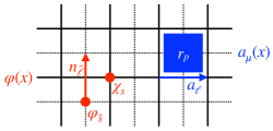
Figure 1: The setting for the field content of our lattice action (4). The solid grid is the primary lattice with sites $s$, links $\ell$, and plaquettes $p$. The dotted grid is the dual lattice with sites $\tilde{s}$, links $\tilde{\ell}$, and plaquettes $\tilde{p}$. The three red fields $\varphi$, $\chi$, and $n$ are associated with the continuum $\varphi$. The two blue fields $a$ and $r$ correspond to the continuum $a_{\mu}$.

The action for our discretization of $N_{f}=1$ QED is

$$S_{N_{f}=1} =\frac{\beta}{2}\left[(da)_{p}-2\pi r_{p}\right]^{2}+\frac{\kappa}{2}\left[(d\varphi)_{\tilde{\ell}}-2\pi n_{\tilde{\ell}}\right]^{2}$$ (4)

$$-i\chi_{s}(dn)_{\star s}+\frac{iQ}{2\pi}\varphi_{\star p}\left[(da)_{p}-2\pi r_{p}\right]-iQa_{\ell}\,n_{\star\ell}$$

where repeated indices are summed and $d$ is the lattice exterior derivative $(d\omega)_{c^{r+1}}=\sum_{c^{r}\in\partial c^{r+1}}\omega_{c^{r}}$ where $c^{r}$ is an $r$-cell, so that, for example, $(d\chi)_{\ell}=\chi_{s+\hat{\ell}}-\chi_{s}$, and $d^{2}=0$. The Hodge star $\star$ maps an $r$-cell $c^{r}$ on the lattice to the $(d-r)$-cell $(\star c)^{d-r}$ on the dual lattice which pierces $c^{r}$. 

The gauge redundancies of the lattice action (4) are

$$a_{\ell} \to a_{\ell}+(d\lambda)_{\ell}+2\pi m_{\ell}\,,\;r_{p}\to r_{p}+(dm)_{p}$$ (5a)

$$\varphi_{\tilde{s}} \to\varphi_{\tilde{s}}+2\pi k_{\tilde{s}}\,,\;n_{\tilde{\ell}}\to n_{\tilde{\ell}}+(dk)_{\tilde{\ell}}$$ (5b)

$$\chi_{s} \to\chi_{s}+Q\lambda_{s}+2\pi h_{s}$$ (5c)

where $\{\lambda_{s}\in\mathbb{R},m_{\ell},k_{\tilde{s}},h_{s}\in\mathbb{Z}\}$ are gauge parameters. They ensure that $\{a,r\}$ and $\{\chi,\varphi,n\}$ describe a $U(1)$ gauge field and a $2\pi$-periodic boson with a conserved winding charge, with the topological properties one expects in the continuum. For example, the instanton number on the spacetime torus $I=-\tfrac{1}{2\pi}\sum_{p}\left[(da)_{p}-2\pi r_{p}\right]=\sum_{p}r_{p}$ is an integer. The path integral over $\chi_{s}$ implies that $(dn)_{\tilde{p}}=0$ on shell, the $\frac{iQ}{2\pi}$ in the lattice action (4) term is the analog of the continuum $\frac{iQ}{2\pi}$ term (3), and the last contribution to the lattice action (4) is necessary to maintain gauge invariance Gorantla et al. (2021).

Given that $\beta=1/(2e^{2}a^{2})$, to get a continuum limit with fixed $Le$, where $L$ is the physical box size $L=Na$, we should take $N\to\infty$ with $\beta/N^{2}$ fixed. While naively one should also set $\kappa=1/(4\pi)$ to reach the continuum (3), this parameter value is not protected by any symmetries of the lattice theory, and can receive some finite renormalization Kosterlitz (1974); Villain (1975); Janke and Nather (1993). Varying $\kappa$ amounts to varying the coefficient of the marginal Thirring term $(\bar{\psi}\gamma^{\mu}\psi)^{2}$.

The lattice action (4) has precisely the desired global symmetries of the continuum (2). There is no continuous $U(1)_{A}$ symmetry, but thanks to the quantization of instanton number, there is a remnant $(\mathbb{Z}_{Q})_{A}$ symmetry that acts as as $\varphi_{\tilde{s}}\to\varphi_{\tilde{s}}+2\pi q/Q$ with $q\in\mathbb{Z}$. This reproduces the expected ABJ chiral anomaly. The $(\mathbb{Z}_{Q})_{\rm e}$ symmetry acts as $a_{\ell}\to a_{\ell}+\frac{2\pi}{Q}v_{\ell}$ with $v\in\mathbb{Z}$ and $dv=0$, also matching the continuum.

To see the ’t Hooft anomaly between $(\mathbb{Z}_{Q})_{\rm e}$ and $(\mathbb{Z}_{Q})_{A}$ on the lattice, it is easiest to linearize the quadratic terms in the action by integrating in auxiliary fields $\zeta_{\ell},\xi_{\tilde{s}}\in\mathbb{R}$ and summing by parts, turning the original action (4) into 

$$S^{\prime}_{N_{f}=1} =\left(\frac{1}{2\kappa}\zeta_{\ell}^{2}+i\zeta_{\ell}\left[(d\varphi)_{\star\ell}-2\pi n_{\star\ell}\right]\right)$$ (6)

$$+\left(\frac{1}{2\beta}\xi_{\star p}^{2}+i\xi_{\star p}\left[(da)_{p}-2\pi r_{p}\right]\right)$$

$$+\frac{iQ}{2\pi}\varphi_{\star p}\left[(da)_{p}-2\pi r_{p}\right]-in_{\star\ell}\left[Qa_{\ell}-(d\chi)_{\ell}\right]\,.$$

The generators of the axial $(\mathbb{Z}_{Q})_{A}$ and electric $(\mathbb{Z}_{Q})_{\rm e}$ symmetries are topological line and local operators on the lattice and dual lattice, respectively:

$$(U_{A})[C]=e^{i\sum_{\ell\in C}\left(a_{\ell}+\frac{2\pi}{Q}\zeta_{\ell}\right)}\,,\;(U_{\rm e})_{\tilde{s}}=e^{i\left(\varphi_{\tilde{s}}+\frac{2\pi}{Q}\xi_{\tilde{s}}\right)}\,,$$ (7)

where $C$ is a closed curve. The fact that $(U_{A})[C]$ is charged under $(\mathbb{Z}_{Q})_{\rm e}$ and $(U_{\rm e})_{p}$ is charged under $(\mathbb{Z}_{Q})_{A}$ encodes the mixed ’t Hooft anomaly of these symmetries, just as in the continuum.

Absence of a sign problem. Direct numerical Monte Carlo with the complex lattice actions (4) and (6) would face a severe sign problem. We now show that this can be eliminated by a change of variables.

Path integrating over $n_{\tilde{\ell}},r_{p}$ in the auxiliary-field action (6) yields constraints that can be solved by setting

$$\zeta_{\ell}=\frac{1}{2\pi}(d\chi)_{\ell}-\frac{Q}{2\pi}a_{\ell}-u_{\ell}\,,\;\xi_{\tilde{s}}=-\frac{Q}{2\pi}\varphi_{\tilde{s}}+t_{\tilde{s}}$$ (8)

with $u_{\ell},t_{\tilde{s}}\in\mathbb{Z}$ which transform as $t_{\tilde{s}}\to t_{\tilde{s}}+Qk_{\tilde{s}}$ and $u_{\ell}\to u_{\ell}+(dh)_{\ell}-Qm_{\ell}$ under discrete gauge transformations. The field $u$ also transforms under $(\mathbb{Z}_{Q})_{\rm e}$ transformations $u_{\ell}\to u_{\ell}-2\pi v_{\ell}/Q$, while $t$ transforms under $(\mathbb{Z}_{Q})_{A}$ as $t_{\tilde{s}}\to t_{\tilde{s}}+q$. Plugging the constraints (8) into the action (6) and dropping total derivatives and integer multiples of $2\pi i$, we obtain an action

$$\frac{1}{2\kappa}\left[\frac{1}{2\pi}(d\chi)_{\ell}-\frac{Q}{2\pi}a_{\ell}-u_{\ell}\right]^{2}+\frac{Q^{2}}{2\beta(2\pi)^{2}}\left[\varphi_{\tilde{s}}-\frac{2\pi t_{\tilde{s}}}{Q}\right]^{2}$$

$$-\frac{i}{2\pi}\left(Qa_{\ell}+2\pi u_{\ell}\right)(d\varphi)_{\star\ell}+it_{\star p}(da)_{p}\,.$$ (9)

Shifting $a\to a+\frac{1}{Q}d\chi-\frac{2\pi}{Q}u$ and dropping a total derivative gives

$$\frac{1}{2\kappa}\left(\frac{Q}{2\pi}a_{\ell}\right)^{2}+\frac{Q^{2}}{2\beta(2\pi)^{2}}\left[\varphi_{\tilde{s}}-\frac{2\pi t_{\tilde{s}}}{Q}\right]^{2}$$

$$-\frac{i}{2\pi}Qa_{\ell}(d\varphi)_{\star\ell}+it_{\star p}\left[(da)_{p}-\frac{2\pi}{Q}(du)_{p}\right]\,,$$ (10)

and subsequently integrating over $a$ yields

$$S_{N_{f}=1,\rm dual} =\frac{\kappa}{2}\left[(d\varphi)_{\tilde{\ell}}-\frac{2\pi}{Q}(dt)_{\tilde{\ell}}\right]^{2}$$ (11)

$$+\frac{1}{2\beta}\left(\frac{Q}{2\pi}\right)^{2}\left(\varphi_{\tilde{s}}-\frac{2\pi}{Q}t_{\tilde{s}}\right)^{2}-\frac{2\pi i}{Q}t_{\star p}(du)_{p}$$

This action describes $Q$ copies (‘universes’ Hellerman et al. (2007); Anber and Poppitz (2018a); Komargodski et al. (2021); Cherman and Jacobson (2021); Cherman et al. (2022); Hellerman and Sharpe (2011); Sharpe (2014, 2019); Robbins et al. (2020); Sharpe (2021)) of a free massive scalar particle, as expected from continuum arguments. Adding a fermion mass term in the original action (2) corresponds to adding $\sum_{\tilde{s}}\cos(\varphi_{\tilde{s}})$ to the dual action (11), which would lead to strong coupling in general.

The sole imaginary term in the dual action (11) involves $u$, but summing over $u$ just gives the constraint $(dt)_{\tilde{\ell}}=0\textrm{ mod }Q$. One can thus avoid the sign problem entirely by proposing updates for $t_{\tilde{s}}$ that satisfy $(dt)_{\tilde{p}}=0\textrm{ mod }Q$ in a Monte Carlo calculation, see Ref. Gattringer et al. (2018) as well as the Supplemental MaterialEvan Berkowitz (2023).

2d QED with $N_{f}=2$. Let us now consider 2d QED with two flavors of massless Dirac fermions $\psi,\hat{\psi}$ with a common charge $Q$. The global flavor symmetry is

$$G_{N_{f}=2}=\frac{SU(2)_{L}\times SU(2)_{R}}{\mathbb{Z}_{2}}\times(\mathbb{Z}_{2})_{G}\times(\mathbb{Z}_{Q})_{A}$$

where $SU(2)_{L,R}$ act on the left and right-handed components of $\psi,\hat{\psi}$, the quotient is by the gauge transformation $\psi,\hat{\psi}\to-\psi,-\hat{\psi}$, $(\mathbb{Z}_{2})_{G}$ is $G$-parity Lee and Yang (1956), and the discrete axial symmetry $(\mathbb{Z}_{Q})_{A}$ is the same as before. There is also a $(\mathbb{Z}_{Q})_{e}$ 1-form symmetry. This model is believed to be equivalent to a self-dual $c=1$ compact boson CFT plus a decoupled massive Schwinger boson Coleman et al. (1975); Coleman (1976); Gepner (1985); Affleck (1986). Mass terms and other perturbations can make this model strongly coupled, and so this field theory has been a popular testing ground for analytic and numeric approaches to confining gauge theories Harada et al. (1994); Shifman and Smilga (1994); Hetrick et al. (1995); Delphenich and Schechter (1997); Narayanan (2012); Lohmayer and Narayanan (2013); Tanizaki and Tachibana (2017); Anber and Poppitz (2018a, b); Armoni and Sugimoto (2019); Misumi et al. (2019); Georgi (2020, 2022); Hirtler and Gattringer (2022); Gattringer et al. (2015); Albergo et al. (2022); Hirtler and Gattringer (2022); Delmastro et al. (2021); Delmastro and Gomis (2023); Dempsey et al. (2023, 2022); Okuda (2023); Itou et al. (2023); Castellanos et al. (2023); Funcke et al. (2023); Ohata (2023a).

Abelian bosonization maps $\psi,\hat{\psi}$ to a pair of $2\pi$-periodic compact bosons $\varphi,\hat{\varphi}$, so we can discretize it in a parallel way to the one-flavor case (4):

$$S_{N_{f}=2} =\frac{\beta}{2}\left[(da)_{p}-2\pi r_{p}\right]^{2}$$ (12)

$$+\frac{\kappa}{2}\left(\left[(d\varphi)_{\star\ell}-2\pi n_{\star\ell}\right]^{2}+\left[(d\hat{\varphi})_{\star\ell}-2\pi\hat{n}_{\star\ell}\right]^{2}\right)$$

$$+\frac{iQ}{2\pi}\left(\varphi_{\star p}+\hat{\varphi}_{\star p}\right)\left[(da)_{p}-2\pi r_{p}\right]$$

$$-iQ(n_{\star\ell}+\hat{n}_{\star\ell})a_{\ell}+in_{\star\ell}(d\chi)_{\ell}+i\hat{n}_{\star\ell}(d\hat{\chi})_{\ell}\,.$$

where $a,\varphi,\hat{\varphi},\chi,\hat{\chi}\in\mathbb{R}$, $n,\hat{n},r\in\mathbb{Z}$, and gauge transformations act as in the one-flavor case (5) plus the analogous shifts of $\hat{\varphi}$, $\hat{n}$, and $\hat{\chi}$ with $\hat{k},\hat{h}\in\mathbb{Z}$.

As before, the lattice parameter $\beta=1/(2e^{2}a^{2})$ and the continuum limit requires the same scaling as in $N_{f}=1$ QED. However, we will see below that now $\kappa=1/4\pi$ is associated with an enhanced symmetry of the action (12), and thus we can set $\kappa=1/4\pi$ on the lattice and be sure that the lattice theory will flow precisely to $N_{f}=2$ charge $Q$ massless QED in the continuum limit without any Thirring terms.

The abelian subgroup of $G_{N_{f}=2}$ is manifestly respected by the two-flavor action (12), and we will argue below that the theory flows to a continuum limit where all of $G_{N_{f}=2}$ is preserved. Following a similar dualization procedure to the $N_{f}=1$ case (see Supplemental MaterialEvan Berkowitz (2023)) we reach

$$S_{N_{f}=2,\textrm{ dual}} =\frac{1}{4\kappa(2\pi)^{2}}\left[(d\sigma)_{\ell}-2\pi u_{\ell}\right]^{2}+i\phi_{\star p}(du)_{p}$$

$$+\frac{\kappa}{4}\left[(d\eta)_{\tilde{\ell}}-\frac{2\pi}{Q}(dt)_{\tilde{\ell}}\right]^{2}-\frac{2\pi i}{Q}\hat{u}_{\ell}(dt)_{\star\ell}$$

$$+\frac{1}{2\beta}\left(\frac{Q}{2\pi}\right)^{2}\left(\eta_{\tilde{s}}-\frac{2\pi}{Q}t_{\tilde{s}}\right)^{2}$$ (13)

where the fields $u,\hat{u},t\in\mathbb{Z}$ emerge during the dualization process, and

$$\sigma=\chi-\hat{\chi}\,,\ \eta=\varphi+\hat{\varphi}\,,\ \phi=\frac{\hat{\varphi}}{2}-\frac{\varphi}{2}-\frac{\pi}{Q}t$$

are real. The gauge redundancies are

$$\sigma_{s} \to\sigma_{s}+2\pi h_{s}\,,\ u_{\ell}\to u_{\ell}+(dh)_{\ell}\,,$$ (14a)

$$\eta_{\tilde{s}} \to\eta_{\tilde{s}}+2\pi k_{\tilde{s}}\,,\ t_{\tilde{s}}\to t_{\tilde{s}}+Qk_{\tilde{s}}\,,$$ (14b)

$$\phi_{\tilde{s}} \to\phi_{\tilde{s}}+2\pi\hat{h}_{\tilde{s}}\,,\ \hat{u}_{\ell}\to\hat{u}_{\ell}+(dw)_{\ell}+Qg_{\ell}\,,$$ (14c)

with all gauge parameters taking values in $\mathbb{Z}$. Finally, the terms with factors of $i$ simply impose constraints [$(du)_{p}=0$ and $(dt)_{\tilde{\ell}}=0$ mod $Q$], and solving these constraints when generating field configurations in a Monte Carlo calculation avoids the sign problem; see again Appendix B.

The dual formulation (13) shows that in the massless limit, our lattice theory decomposes into two decoupled sectors. The top line of (13) is simply the modified Villain discretization of the compact boson $\sigma$. But when we set $\kappa=1/(4\pi)$, the effective radius of $\sigma$ makes the theory self-dual under Poisson resummation on $u_{\ell}$, which implements T-duality on the lattice Gorantla et al. (2021). This implies the existence of a topological line operator which is absent for generic $\kappa$ Kapustin and Tikhonov (2009); Choi et al. (2022), so that the $\kappa=1/(4\pi)$ point is protected by an enhanced symmetry against quantum corrections! The continuum limit is thus guaranteed to be the self-dual $c=1$ compact boson CFT with non-abelian $[SU(2)\times SU(2)]/\mathbb{Z}_{2}$ global symmetry. The decoupled ‘Schwinger boson’ QFT in the lower lines of the dual action (13) matches the remaining symmetries:

$$(\mathbb{Z}_{2})_{G} : \eta_{\tilde{s}}\to-\eta_{\tilde{s}},\ \phi_{\tilde{s}}\to\phi_{\tilde{s}}+\frac{2\pi}{Q}t,$$

$$\hat{u}_{\ell}\to-\hat{u}_{\ell}+u_{\ell},\ t_{\tilde{s}}\to-t_{\tilde{s}}$$ (15)

$$(\mathbb{Z}_{Q})_{A} : \eta_{\tilde{s}}\to\eta_{\tilde{s}}+\frac{2\pi q}{Q},\ t_{\tilde{s}}\to t_{\tilde{s}}+q_{\tilde{s}},q\in\mathbb{Z}$$

$$(\mathbb{Z}_{Q})_{e} : \hat{u}_{\ell}\to\hat{u}_{\ell}+\frac{2\pi}{Q}v_{\ell},\ v_{\ell}\in\mathbb{Z},(dv)_{p}=0\,.$$

Chiral gauge theory. We now turn to a popular example Halliday et al. (1986); Eichten and Preskill (1986); Narayanan and Neuberger (1997); Kikukawa et al. (1998, 1997); Bhattacharya et al. (2006); Giedt and Poppitz (2007); Chen et al. (2013); Poppitz and Shang (2007, 2009, 2010); Chen et al. (2013); Wang and Wen (2023, 2019); Tong (2022); Zeng et al. (2022); Wang and You (2022); Wang (2022); Seifnashri (2023) of a 2d abelian chiral gauge theory, namely the ‘$3450$’ model, which has two left-handed Weyl fermions $\psi_{L},\hat{\psi}_{L}$ coupled to a $U(1)$ gauge field with charges $3,4$ as well as two right-handed Weyl fermions $\psi_{R},\hat{\psi}_{R}$ with charges $5,0$.  This QFT satisfies the gauge anomaly cancellation condition $(Q_{L})^{2}+(\hat{Q}_{L})^{2}=(Q_{R})^{2}+(\hat{Q}_{R})^{2}$ as well as the gravitational ’t Hooft anomaly cancellation condition on the left and right central charges $c_{L}=c_{R}$. After repackaging the matter into two Dirac fermions $\psi=(\psi_{R},\psi_{L}){}^{\top},\hat{\psi}=(\hat{\psi}_{R},\hat{\psi}_{L}){}^{\top}$, the gauge field couples to the vector and axial currents of $\psi,\hat{\psi}$ with charges $Q_{V}=8,Q_{A}=-2,\hat{Q}_{V}=4,\hat{Q}_{A}=4\,,$ and the gauge anomaly cancellation condition becomes $Q_{V}Q_{A}+\hat{Q}_{V}\hat{Q}_{A}=0$.

We will study the variant of the $3450$ model with a gauged $(-1)^{F}$ symmetry to avoid dealing with the Arf invariant Thorngren (2020); Karch et al. (2019). Our discretization takes the form

$$S_{3450} =\frac{\beta}{2}\left[(da)_{p}-2\pi r_{p}\right]^{2}$$ (16)

$$+\frac{\kappa}{2}\bigg{(}\left[(d\varphi)_{\tilde{\ell}}-Q_{A}a_{f(\tilde{\ell})}-2\pi n_{\tilde{\ell}}\right]^{2}$$

$$\phantom{=\frac{\kappa}{2}\bigg{(}}+\left[(d\hat{\varphi})_{\tilde{\ell}}-\hat{Q}_{A}a_{f(\tilde{\ell})}-2\pi\hat{n}_{\tilde{\ell}}\right]^{2}\bigg{)}$$

$$+\frac{i}{2\pi}\left(Q_{V}\varphi_{\star p}+\hat{Q}_{V}\hat{\varphi}_{\star p}\right)\left[(da)_{p}-2\pi r_{p}\right]$$

$$-i(Q_{V}n_{\star\ell}+\hat{Q}_{V}\hat{n}_{\star\ell})a_{\ell}+in_{\star\ell}(d\chi)_{\ell}+i\hat{n}_{\star\ell}(d\hat{\chi})_{\ell}$$

$$-ir_{f(\star s)}(Q_{A}\chi_{s}+\hat{Q}_{A}\hat{\chi}_{s})\,.$$

where $f:s\to s+\tfrac{1}{2}(\hat{x}+\hat{y})$ shifts cells from the lattice to the dual lattice, and the gauge redundancies are

$$a_{\ell} \to a_{\ell}+(d\lambda)_{\ell}+2\pi m_{\ell}\,,\;r_{p}\to r_{p}+(dm)_{p}$$ (17)

$$\varphi_{\tilde{s}} \to\varphi_{\tilde{s}}+Q_{A}\lambda_{f(\tilde{s})}+2\pi k_{\tilde{s}},\hat{\varphi}_{\tilde{s}}\to\hat{\varphi}_{\tilde{s}}+\hat{Q}_{A}\lambda_{f(\tilde{s})}+2\pi\hat{k}_{\tilde{s}}$$

$$n_{\tilde{\ell}} \to n_{\tilde{\ell}}+(dk)_{\tilde{\ell}}-Q_{A}m_{f(\tilde{\ell})}\,,\hat{n}_{\tilde{\ell}}\to\hat{n}_{\tilde{\ell}}+(d\hat{k})_{\tilde{\ell}}-\hat{Q}_{A}m_{f(\tilde{\ell})}$$

$$\chi_{s} \to\chi_{s}+Q_{V}\lambda_{s}+2\pi h_{s}\,,\hat{\chi}_{s}\to\hat{\chi}_{s}+\hat{Q}_{V}\lambda_{s}+2\pi\hat{h}_{s}\,.$$

Modulo $2\pi i$ and total derivative terms, the gauge variation of $S_{3450}$ is

$$\Delta S_{3450}=i(Q_{V}Q_{A}+\hat{Q}_{V}\hat{Q}_{A})\Bigg{[}m_{\ell}a_{f^{-1}(\star\ell)}$$ (18)

$$+\lambda_{s}\Big{(}\frac{1}{2\pi}(da)_{f^{-1}(\star s)}-r_{f^{-1}(\star s)}-r_{f(\star s)}-(dm)_{f(\star s)}\Big{)}\Bigg{]}$$

which vanishes precisely when the charges satisfy the anomaly cancellation condition.

The presence of the function $f$ in (16) appears to break $\mathbb{Z}_{4}$ lattice rotation symmetry. Also, $\textrm{Im}S_{3450}\neq 0$, leading to an apparent sign problem. However, following the same method as in $N_{f}=1,2$ vector-like QED, one can derive (see Supplemental MaterialEvan Berkowitz (2023)) a dual representation which both avoids the sign problem and shows that $\mathbb{Z}_{4}$ lattice rotation symmetry is actually preserved, since it is manifest in the dual variables. This dual representation can be written as

$$S_{3450,\textrm{ dual}}=\frac{\kappa}{2}\frac{1}{5}\left((d\phi)_{\star\ell}-2\pi v_{\star\ell}\right)^{2}\\ +\frac{1}{2\kappa}\frac{1}{20(2\pi)^{2}}\left(2(d\psi)_{\tilde{\ell}}-2\pi((dy)_{\tilde{\ell}}-4v_{\tilde{\ell}})\right)^{2}\\ +\frac{1}{2\beta}\frac{1}{(2\pi)^{2}}(4\phi_{\tilde{s}}+2\psi_{\tilde{s}}-2\pi y_{\tilde{s}})^{2}\\ +i\sigma_{\star\tilde{p}}(dv)_{\tilde{p}}-i\pi\hat{n}_{\star\tilde{\ell}}(dy)_{\tilde{\ell}}-2\pi i\frac{4}{5}v_{\star\ell}v_{f(\ell)}\,.$$ (19)

where $v,y,\hat{n}\in\mathbb{Z}$ and

$$\psi_{\tilde{s}}=-\chi_{f(\tilde{s})}+2\hat{\chi}_{f(\tilde{s})},\ \phi_{\tilde{s}}=2\varphi_{\tilde{s}}+\hat{\varphi}_{\tilde{s}}\,.$$ (20)

which are $U(1)$-gauge-invariant. When $\psi_{\tilde{s}}\to\psi_{\tilde{s}}+2\pi q_{\tilde{s}}$ and $\phi_{\tilde{s}}\to\phi_{\tilde{s}}+2\pi b_{\tilde{s}}$, the discrete fields shift as $v_{\tilde{\ell}}\to v_{\tilde{\ell}}+(db)_{\tilde{\ell}}$ and $y_{\tilde{s}}\to y_{\tilde{s}}+4b_{\tilde{s}}+2q_{\tilde{s}}$. The first two terms in the last line of Eq. (19) yield constraints $(dv)_{\tilde{p}}=0$ and $(dy)_{\tilde{\ell}}=0$ mod $2$. But when $dv=0$ the last term can be shown to be a total derivative (see Appendix D) and can be dropped, giving a sign-problem-free formulation with a manifest $\mathbb{Z}_{4}$ rotation symmetry.

Outlook. We leveraged recent advances in the understanding of anomalies on the lattice Sulejmanpasic and Gattringer (2019); Gorantla et al. (2021); Fazza and Sulejmanpasic (2023); Cheng and Seiberg (2023); Seifnashri (2023) to construct symmetry-preserving discretizations of massless vector-like and chiral abelian gauge theories in $d=2$ spacetime dimensions. The vector-like and chiral symmetries act just as locally at finite lattice spacing as they do in the continuum, and all of the ABJ and ’t Hooft anomalies are reproduced on the lattice. These discretizations evade the Nielsen-Ninomiya theorem essentially because they directly discretize the fermion determinant $\det\not{D}$ rather than the fermion matrix $\not{D}$ itself. Finally, despite the fact that the lattice actions we construct are complex, we have shown that the resulting sign problems can be avoided by judicious choices of dual variables.

Our results open many directions for future work. Numerical lattice calculations using this formalism can be used to explore strongly-coupled regions in parameter space. It would be interesting to see if our approach can be generalized to $d>2$, for example by taking advantage of advances in the understanding of continuum bosonization in $d=3$ Aharony (2016); Seiberg et al. (2016); Karch and Tong (2016); Karch et al. (2017); Wang et al. (2017); Hsin and Seiberg (2016); Karch et al. (2018) and the development of symmetry-preserving discretizations of Chern-Simons terms Jacobson and Sulejmanpasic (2023). It would also be nice to see if generalizations of our construction can preserve non-Abelian chiral symmetries at finite lattice spacing Luscher (2000); Wen (2013); BenTov (2015); Ayyar and Chandrasekharan (2015, 2016a, 2016b); DeMarco and Wen (2017); Razamat and Tong (2021); Catterall (2023a). Finally, to get inspiration towards constructing more direct symmetry-preserving fermion discretizations, one can compute the discretized Dirac operators corresponding to our representations of the fermion determinant $\det\not{D}$.

Acknowledgements. We thank Shi Chen, Erich Poppitz, Srimoyee Sen and Misha Shifman for helpful discussions, are grateful to Srimoyee Sen and Juven Wang for comments on a draft, and thank the audience at the Simons Foundation “Confinement and QCD Strings” 2023 Annual Meeting for helpful remarks during a presentation of our results. The work of EB and AC was performed in part at the Aspen Center for Physics, which is supported by National Science Foundation grant PHY-2210452. AC was also supported by a Simons Foundation Grant No. 994302 as part of the Simons Collaboration on Confinement and the QCD String. TJ is supported by a Julian Schwinger Fellowship from the Mani L. Bhaumik Institute for Theoretical Physics at UCLA, and thanks NCSU for hospitality during the completion of this work.

Appendix A Hamiltonian Formulation

To construct the Hamiltonian we follow the discussion of Ref. Fazza and Sulejmanpasic (2023) (see Section 3.5 therein for a parallel discussion). We go to Lorentzian signature, take time to be continuous, drop the time-like integer-valued fields in the lattice action (4), and assume that space is discretized on a lattice with periodic boundary conditions. The Lagrangian density becomes

$$\mathcal{L}=\frac{\kappa}{2}\dot{\varphi}_{\tilde{s}}^{2}-\frac{\kappa}{2}[(d\varphi)_{\tilde{\ell}}-2\pi n_{\tilde{\ell}}]^{2}+\frac{\beta}{2}\dot{a}^{2}_{\ell}-\frac{Q}{2\pi}\varphi_{\star\ell}\dot{a}_{\ell}+\chi_{s}\dot{n}_{\star s}$$ (21)

Note that on the 1d lattice $\star\ell=\tilde{s},\star s=\tilde{\ell}$. The canonical momenta (which live on the duals of the cells of their respective fields) can thus be written as

$$(\Pi_{\varphi})_{\ell} =\kappa\dot{\varphi}_{\star\ell}\,,\;(\Pi_{a})_{\tilde{s}}=\beta\dot{a}_{\ell}-\frac{Q}{2\pi}$$ (22)

$$(\Pi_{n})_{s} =\chi_{s}\,,\;(\Pi_{\chi})_{\tilde{\ell}}=0$$ (23)

The lower two lines are second-class constraints. They can be taken into account using Dirac brackets, which lead us to the quantum Hamiltonian

$$\mathbf{H} =\frac{1}{2\kappa}(\mathbf{\Pi_{\varphi}})_{\ell}^{2}+\frac{1}{2\beta}\left[(\mathbf{\Pi}_{a})_{\tilde{s}}+\frac{Q}{2\pi}\bm{\varphi}_{\tilde{s}}\right]^{2}$$

$$+\frac{\kappa}{2}[(d\bm{\varphi})_{\tilde{\ell}}-2\pi\mathbf{n}_{\tilde{\ell}}]^{2}$$ (24)

where $\bm{\varphi},\mathbf{\Pi_{\varphi}},\mathbf{a},\mathbf{\Pi}_{a},\mathbf{n},\bm{\chi}$ are operators with the commutation relations

$$[\bm{\varphi}_{\tilde{s}},(\mathbf{\Pi_{\varphi}})_{\ell}] =i\delta_{\tilde{s},\star\ell},$$

$$[\mathbf{a}_{\ell},(\mathbf{\Pi}_{a})_{\tilde{s}}] =i\delta_{\ell,\star{\tilde{s}}},$$ (25)

$$[\mathbf{n}_{\tilde{\ell}},\bm{\chi}_{s}] =i\delta_{\star\tilde{\ell},s},$$

Gauge operators. In the Hamiltonian formalism the gauge redundacies must be imposed as constraints. We have four such redundancies: compactness of $\bm{\chi}$, compactness of $\bm{\varphi}$, small gauge transformations of $\mathbf{a}$ and $\bm{\chi}$, and large gauge transformations that ensure that the gauge group is $U(1)$ and not $\mathbb{R}$. These transformations will be associated with four operators $\mathbf{G}_{\chi},\mathbf{G}_{\varphi},\mathbf{G}_{\rm small},\mathbf{G}_{\rm large}$ which have to act like identity operators on all physical states.

The $2\pi$ shifts of $\chi$ are generated by

$$\mathbf{G}_{\chi}=[\{s_{\tilde{\ell}}\}]=e^{2\pi i\sum_{\tilde{\ell}}s_{\tilde{\ell}}\mathbf{n}_{\tilde{\ell}}}\,.$$ (26)

where $s_{\tilde{\ell}}\in\mathbb{Z}$. Therefore $\mathbf{n}_{\tilde{\ell}}$ must have an integer spectrum.

The compactness condition for $\bm{\varphi}$ is associated with the transformation $\bm{\varphi}_{\tilde{s}}\to\bm{\varphi}_{\tilde{s}}+2\pi k_{\tilde{s}},\mathbf{n}_{\tilde{\ell}}\to\mathbf{n}_{\tilde{\ell}}+(dk)_{\tilde{\ell}},(\mathbf{\Pi}_{a})_{\tilde{s}}\to(\mathbf{\Pi}_{a})_{\tilde{s}}-\frac{Q}{2\pi}k_{\tilde{s}}$ with $k_{\tilde{s}}\in\mathbb{Z}$, which is generated by

$$\mathbf{G}_{\varphi}[\{k\}]=\exp\left[i\sum_{\ell}2\pi k_{\star\ell}\left((\mathbf{\Pi_{\varphi}})_{\ell}-\frac{Q}{2\pi}\mathbf{a}_{\ell}-\frac{1}{2\pi}(d\bm{\chi})_{\ell}\right)\right]$$ (27)

Therefore the operator

$$\mathbf{q}_{\ell}=(\mathbf{\Pi_{\varphi}})_{\ell}+\frac{Q}{2\pi}\mathbf{a}_{\ell}-\frac{1}{2\pi}(d\bm{\chi})_{\ell}$$ (28)

must have an integer spectrum. Its commutation relations are

$$[\mathbf{q}_{\ell},\bm{\varphi}_{\tilde{s}}] =i\delta_{\tilde{s},\star\ell},$$

$$[\mathbf{q}_{\ell},(\mathbf{\Pi}_{a})_{\tilde{s}}] =\frac{iQ}{2\pi}\delta_{\ell,\star{\tilde{s}}},$$ (29)

$$[\mathbf{q}_{\ell},\mathbf{n}_{\tilde{\ell}}] =\frac{i}{2\pi}\left(\delta_{f(\ell),\tilde{\ell}}-\delta_{f^{-1}(\ell),\tilde{\ell}}\right)$$

where $f(\ell)$ is a positive translation by half a lattice unit, which takes the lattice to the dual lattice.

Continuous (‘small’) gauge transformations $\mathbf{a}\to\mathbf{a}+d\lambda,\bm{\chi}\to\bm{\chi}+Q\lambda$ are generated by

$$\mathbf{G}_{\rm small}(\{\lambda\})=\exp\left[i\sum_{\ell}(d\lambda)_{\ell}(\mathbf{\Pi}_{a})_{\ell}-iQ\sum_{s}\lambda_{s}\mathbf{n}_{\star s}\right]$$ (30)

where ${\lambda_{s}}\in\mathbb{R}$. This yields the Gauss law constraint

$$(d\mathbf{\Pi}_{a})_{\tilde{\ell}}+Q\mathbf{n}_{\tilde{\ell}}=0.$$ (31)

Finally, the large gauge transformations $(\mathbf{\Pi}_{a})_{\ell}\to(\mathbf{\Pi}_{a})_{\ell}+2\pi m_{\ell}$ are generated by

$$\mathbf{G}_{\rm large}(\{m\})=e^{i\sum_{\ell}2\pi m_{\ell}(\mathbf{\Pi}_{a})_{\ell}}\,,\;m_{\ell}\in\mathbb{Z}$$ (32)

which implies that $\mathbf{\Pi}_{a}$ must have an integer spectrum.

Symmetry operators. The two internal global symmetries of our Hamiltonian are associated with the following operators. The $\mathbb{Z}_{Q}$ chiral symmetry is generated by the line operator

$$\mathbf{U}_{k}(L) =\exp\left[\frac{2\pi ik}{Q}\sum_{\ell\in L}\left((\mathbf{\Pi_{\varphi}})_{\ell}+\frac{Q}{2\pi}(\mathbf{\Pi}_{a})_{\ell}\right)\right]$$ (33)

$$=e^{\frac{2\pi ik}{Q}\sum_{\ell}\mathbf{q}_{\ell}}$$

where $L$ is all of space (that is, a time slice). This means that $\mathbf{q}_{\ell}$ is a charge density operator (which manages to exist in this case despite the fact that chiral symmetry is discrete) and $\mathbf{Q}=\sum_{\ell}\mathbf{q}_{\ell}$ is the total charge operator. The equation of motion of $\mathbf{q}$ is $\dot{\mathbf{q}}=i[\mathbf{H},\mathbf{q}]=0$, so $\mathbf{U}_{k}(L)$ is conserved, and the coefficient in front of $\mathbf{Q}$ is quantized thanks to the requirement that $\mathbf{U}_{k}(L)$ must commute with $\mathbf{G}_{\rm large}$.

The $\mathbb{Z}_{Q}$ $1$-form symmetry is generated by the local operator

$$\mathbf{V}_{w}(\tilde{s})=e^{\frac{2\pi i}{Q}(\mathbf{\Pi}_{a})_{\tilde{s}}}.$$ (34)

The coefficient in the exponent must be quantized so that $[\mathbf{V}_{w},\mathbf{G}_{\varphi}]=0$, and it is topological thanks to the Gauss law.

The ’t Hooft anomaly is encoded in the fact that these symmetry operators do not commute

$$\mathbf{U}_{k}(L)\mathbf{V}_{w}(\tilde{s})=e^{\frac{2\pi ikw}{Q}}\mathbf{V}_{w}(\tilde{s})\mathbf{U}_{k}(L)$$ (35)

Therefore (24) provides a Hamiltonian discretization of the charge $Q$ Schwinger model which encodes all of its continuum internal symmetries and anomalies.

Appendix B Trading sign problems for constraints

To make our presentation self-contained, we give a brief discussion of how simple constraints can be taken into account in Monte Carlo calculations without sign problems, although everything we explain below is well-known. See, for example, Ref. Gattringer et al. (2018).

Consider a lattice field theory with an action $S$ where the only term where the field $u$ appears is

$$S\ni\frac{2\pi i}{Q}u_{\ell}(dt)_{\ell}$$ (36)

where $Q\in\mathbb{N},u_{\ell}\in\mathbb{Z},t_{s}\in\mathbb{Z}$. The dual one-flavor (11), two-flavor (13), and 3450 (19) models all have this character.

Because it is purely imaginary, direct Monte Carlo evaluation of the QFT path integral based on importance-sampling with this term as part of the action suffers from a sign problem. However, the path integral over $u$ can be done analytically and yields a delta function setting $(dt)_{\ell}=0\textrm{ mod }Q$. If we can make proposals that maintain this constraint but are otherwise ergodic we will consider all supported configurations of $t_{s}$ and avoid the sign problem caused by the phase (36).

On a torus, where all of the integer cohomology groups are torsion-free, we can solve the constraint by writing

$$t_{s}=x+Qy_{s}$$ (37)

$x,y_{s}\in\mathbb{Z}$ and $x$ is a constant so that $(dx)_{\ell}=0$. Note that this decomposition is not unique. For example, we can shift $x$ by $Q$ and all $y$s by $-1$ without changing $t$. But this decomposition helps us offer two kinds of proposals which together reach all constraint-satisfying configurations.

The first proposal is a global update of $x$. We randomly pick a site-independent integer $\Delta x\in[-X,+X]$ with $X\in\mathbb{Z}$, and Metropolis test $t_{s}\to t_{s}+\Delta x$ for all sites $s$ simultaneously.

The second is a local update of $y$ which we can sweep across the lattice. On a particular site $s$ we pick an integer $\Delta y_{s}\in[-Y,+Y]$ with $Y\in\mathbb{Z}$, and test $t_{s}\to t_{s}+Q\Delta y_{s}$.

An ergodic algorithm should offer proposals of both kinds, and their relative frequency may be adjusted to control autocorrelation times. The algorithm parameters $X$ and $Y$, or more generally the distributions for $\Delta x$ and $\Delta y_{s}$, may be adjusted to optimize acceptance and thermalization.

Similarly, suppose the action includes a term

$$S\ni i\eta_{p}(dn)_{p}$$ (38)

where $\eta_{p}\in\mathbb{R},n_{\ell}\in\mathbb{Z}$, and $\eta$ does not appear in any other terms. The dual 3450 action (19) has a term of this character. Integrating out $\eta$ yields the constraint $(dn)_{p}=0$.

The field $n_{\ell}$ may be split into a closed $1$-form $w_{\ell}\in\mathbb{Z}$ and an exact $1$-form $(dz)_{\ell}\in\mathbb{Z}$

$$n_{\ell}=w_{\ell}+(dz)_{\ell}.$$ (39)

As we will see below, updates of $z$ are local, while updates of $w$ ‘wrap’ around cycles of the torus. Again, for a given field configuration the decomposition above is not unique.

As before, we offer two kinds of proposals, depicted in Figure 2, which together reach all constraint-satisfying configurations of $n$.

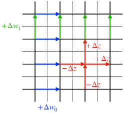
Figure 2: Two kinds of proposals for $n_{\ell}$ which satisfy $(dn)_{p}=0$. In red is a local update which is an exact form $dz$ of a single-site 0-form. The blue and green updates are of whole strips of links, and are closed because opposite edges of a plaquette contribute inversely to $(dn)_{p}$.

We first an offer update of the closed $1$-form $w$. We update a torus-wrapping strip of parallel links at once, as shown by the blue and green updates in Figure 2. We pick a single integer $\Delta w\in[-W,+W]$ with $W\in\mathbb{Z}$ and Metropolis test $n_{\ell}\to n_{\ell}+\Delta w$ for all the links on the strip. We can sweep this update across all the strips of the lattice in either orientation.

The second proposal offers a local update to the exact $1$-form $dz$. We pick $\Delta z\in[-Z,+Z]$ with $Z\in\mathbb{Z}$ and a site $s$ and build a 0-form $z$ that vanishes everywhere except at $s$ where it is $-\Delta z$. We propose $n_{\ell}\to n_{\ell}+(dz)_{\ell}$, which amounts to the simultaneous proposal

$$n_{s,\hat{0}} \to n_{s,\hat{0}}+\Delta z n_{s-\hat{0},\hat{0}} \to n_{s-\hat{0},\hat{0}}-\Delta z$$

$$n_{s,\hat{1}} \to n_{s,\hat{1}}+\Delta z n_{s-\hat{1},\hat{1}} \to n_{s-\hat{1},\hat{1}}-\Delta z$$ (40)

where $\hat{0}$ and $\hat{1}$ are unit vectors in the positive time and space directions.

An ergodic algorithm should offer proposals of both kinds, and as before their relative frequency may be adjusted to control autocorrelation times. The distributions of $\Delta w$ and $\Delta z$ may be adjusted to optimize performance, for example by changing $W$ and $Z$.

The constrained update algorithms presented here are only existence proofs of methods which evade the sign problem. They may have long autocorrelation times, especially given that some of the proposals touch a number of variables growing with the lattice size $N$ and may be often rejected. Famously, worm algorithms Prokof’ev et al. (1998); Prokof’ev and Svistunov (2001) can quickly decorrelate worldline formulations which have closed-loop constraints; it would be interesting to try and adapt these powerful tools to our actions.

Appendix C Dualizing $N_{f}=2$ QED

We start with the action (12), linearize the gauge and scalar kinetic terms using auxiliary fields, and sum over $n,\hat{n},r$ to find

$$\frac{1}{2\kappa}\left(\frac{N}{2\pi}\right)^{2}\Bigg{[}\left(a_{\ell}-\frac{1}{N}(d\chi)_{\ell}-\frac{2\pi}{N}y_{\ell}\right)^{2}\\ +\left(a_{\ell}-\frac{1}{N}(d\hat{\chi})_{\ell}-\frac{2\pi}{N}\hat{u}_{\ell}\right)^{2}\Bigg{]}\\ +\frac{1}{2\beta}\left(\frac{N}{2\pi}\right)^{2}\left(\varphi_{\tilde{s}}+\hat{\varphi}_{\tilde{s}}-\frac{2\pi}{N}t_{\tilde{s}}\right)^{2}+ia_{\ell}(dt)_{\star p}\\ -\frac{i}{2\pi}(Na_{\ell}+2\pi y_{\ell})(d\varphi)_{\star\ell}-\frac{i}{2\pi}(Na_{\ell}+2\pi\hat{u}_{\ell})(d\hat{\varphi})_{\star\ell}\,,$$ (41)

where $y,\hat{u},t\in\mathbb{Z}$. Doing the Gaussian integral over $a$ gives

$$\frac{1}{4\kappa}\frac{1}{(2\pi)^{2}}\left((d\chi)_{\ell}-(d\hat{\chi})_{\ell}-2\pi(y_{\ell}-\hat{u}_{\ell})\right)^{2}\\ +\frac{\kappa}{4}\left((d\varphi)_{\tilde{\ell}}+(d\hat{\varphi})_{\tilde{\ell}}-\frac{2\pi}{N}(dt)_{\tilde{\ell}}\right)^{2}\\ +\frac{1}{2\beta}\left(\frac{N}{2\pi}\right)^{2}\left(\varphi_{\tilde{s}}+\hat{\varphi}_{\tilde{s}}-\frac{2\pi}{N}t_{\tilde{s}}\right)^{2}\\ -\frac{i}{2}(y_{\ell}-\hat{u}_{\ell})((d\varphi)_{\star\ell}-(d\hat{\varphi})_{\star\ell})-\frac{i}{2}\frac{2\pi}{N}(y_{\ell}+\hat{u}_{\ell})(dt)_{\star\ell}$$ (42)

after dropping total derivatives and multiples of $2\pi i$. Now let us define $\sigma=\chi-\hat{\chi}$, $\eta=\varphi+\hat{\varphi}$, $\phi=\frac{\hat{\varphi}}{2}-\frac{\varphi}{2}-\frac{\pi t}{N}$, $u=y-\hat{u}$.

$$\frac{1}{4\kappa}\frac{1}{(2\pi)^{2}}\left((d\sigma)_{\ell}-2\pi u_{\ell}\right)^{2}\\ +\frac{\kappa}{4}\left((d\eta)_{\tilde{\ell}}-\frac{2\pi}{N}(dt)_{\tilde{\ell}}\right)^{2}+\frac{1}{2\beta}\left(\frac{N}{2\pi}\right)^{2}\left(\eta_{\tilde{s}}-\frac{2\pi}{N}t_{\tilde{s}}\right)^{2}\\ +iu_{\ell}(d\phi)_{\star\ell}-\frac{2\pi i}{N}\hat{u}_{\ell}(dt)_{\star\ell}$$ (43)

which is the result (13). The first line is the modified Villain formulation of a compact scalar. If we had started with the free-fermion radius $\kappa=\frac{1}{4\pi}$, we end up with an effective radius $\tilde{\kappa}=\frac{1}{2\kappa}\frac{1}{(2\pi)^{2}}=\frac{1}{2\pi}$, which is the self-dual radius.

For completeness, we note the dual description of the fermion mass terms:

$$\cos(\varphi)\to\cos\left(\frac{\eta}{2}-\phi-\frac{\pi}{N}t\right)$$ (44)

and

$$\cos(\hat{\varphi})\to\cos\left(\frac{\eta}{2}+\phi+\frac{\pi}{N}t\right)\,.$$ (45)

As a result, a flavor-symmetric mass deformation becomes

$$\cos(\varphi)+\cos(\tilde{\varphi})\to 2\cos\left(\frac{\eta}{2}\right)\cos\left(\phi+\frac{\pi}{N}t\right)\,.$$ (46)

Note this is respects the $2\pi$ periodicity because when $\eta\to\eta+2\pi k$ and $t\to t+Nk$, both factors pick up a sign $(-1)^{k}$ which squares away. If we turn on a theta angle this is modified to $\cos(\frac{\eta}{2}+\frac{\theta}{2})\cos(\phi+\frac{\pi}{N}t)$.

Appendix D Dualizing the 3450 model

Let us write the action of the 3450 model using (real) auxiliary fields $\zeta,\hat{\zeta},\xi$:

$$S=\frac{1}{2\kappa}\zeta_{\star\tilde{\ell}}^{2}+i\zeta_{\star\tilde{\ell}}[(d\varphi)_{\tilde{\ell}}-Q_{A}\,a_{f(\tilde{\ell})}-2\pi n_{\tilde{\ell}}]\\ +\frac{1}{2\kappa}\hat{\zeta}_{\star\tilde{\ell}}^{2}+i\hat{\zeta}_{\star\tilde{\ell}}[(d\hat{\varphi})_{\tilde{\ell}}-\hat{Q}_{A}\,a_{f(\tilde{\ell})}-2\pi\hat{n}_{\tilde{\ell}}]\\ +\frac{1}{2\beta}\xi_{\star p}^{2}+i\left(\xi_{\star p}+\frac{1}{2\pi}(Q_{V}\varphi_{\star p}+\hat{Q}_{V}\hat{\varphi}_{\star p})\right)[(da)_{p}-2\pi r_{p}]\\ -i(Q_{V}n_{\star\ell}+\hat{Q}_{V}\hat{n}_{\star\ell})a_{\ell}+in_{\star\ell}(d\chi)_{\ell}+i\hat{n}_{\star\ell}(d\hat{\chi})_{\ell}\\ -ir_{p}(Q_{A}\chi_{f^{-1}(\star p)}+\hat{Q}_{A}\hat{\chi}_{f^{-1}(\star p)})\,.$$ (47)

Summing over $r_{p}\in\mathbb{Z}$ sets

$$\xi_{\star p}=-\frac{1}{2\pi}\Big{(}Q_{V}\varphi_{\star p}+\hat{Q}_{V}\hat{\varphi}_{\star p}\\ +Q_{A}\chi_{f^{-1}(\star p)}+\hat{Q}_{A}\hat{\chi}_{f^{-1}(\star p)}-2\pi y_{\star p}\Big{)}\,,$$ (48)

where $y_{\tilde{\ell}}\in\mathbb{Z}$. Plugging this back into the action and integrating out the gauge field $a_{\ell}$ allows us to solve for $\zeta$:

$$\zeta_{\star\tilde{\ell}}=\frac{1}{Q_{A}}\Big{[}-\hat{Q}_{A}\hat{\zeta}_{\star\tilde{\ell}}-\frac{1}{2\pi}(Q_{A}(d\chi)_{\star\tilde{\ell}}+\hat{Q}_{A}(d\hat{\chi})_{\star\tilde{\ell}})\\ +(dy)_{f(\star\tilde{\ell})}-Q_{V}n_{f(\star\tilde{\ell})}-\hat{Q}_{V}\hat{n}_{f(\star\tilde{\ell})}\Big{]}\,.$$ (49)

If we plug this back into the action and perform a field redefinition $\hat{\zeta}_{\ell}\to\hat{\zeta}_{\ell}-\frac{1}{2\pi}(d\hat{\chi})_{\ell}$, we land on

$$S=\frac{1}{2\beta}\frac{1}{(2\pi)^{2}}\xi_{\tilde{s}}^{2}+\frac{1}{2\kappa}\left[\hat{\zeta}_{\ell}-\frac{1}{2\pi}(d\hat{\chi})_{\ell}\right]^{2}\\ +\frac{1}{2\kappa}\frac{\hat{Q}_{A}^{2}}{Q_{A}^{2}}\left[\hat{\zeta}_{\ell}+\frac{Q_{A}}{\hat{Q}_{A}}\frac{(d\chi)_{\ell}}{2\pi}-\frac{(dy)_{f(\ell)}+u_{f(\ell)}}{\hat{Q}_{A}}\right]^{2}\\ -i\frac{\hat{\zeta}_{\ell}}{Q_{A}}\left[Q_{A}(d\hat{\varphi})_{\star\ell}-\hat{Q}_{A}(d\varphi)_{\star\ell}+2\pi\frac{\hat{Q}_{A}}{Q_{V}}u_{\star\ell}\right]\\ +\frac{i}{Q_{A}}u_{f(\ell)}[(d\varphi)_{\star\ell}-2\pi n_{\star\ell}]+\frac{2\pi i}{Q_{A}}(dy)_{f(\ell)}n_{\star\ell}\,,$$ (50)

with $\xi$ set to its value in (48), and for notational convenience we have defined

$$u_{\tilde{\ell}}\equiv Q_{V}n_{\tilde{\ell}}+\hat{Q}_{V}\hat{n}_{\tilde{\ell}}=\frac{Q_{V}}{\hat{Q}_{A}}(\hat{Q}_{A}n_{\tilde{\ell}}-Q_{A}\hat{n}_{\tilde{\ell}})\,,$$ (51)

where the second equality follows from the anomaly-free condition. Note this is not a $GL(2,\mathbb{Z})$ change of basis, and we have to remember that $u_{\tilde{\ell}}\in Q_{V}\mathbb{Z}+\hat{Q}_{V}\mathbb{Z}$. The integral over $\hat{\zeta}$ is Gaussian. To simplify the calculation let us define

$$\phi_{\tilde{s}} =Q_{V}\varphi_{\tilde{s}}+\hat{Q}_{V}\hat{\varphi}_{\tilde{s}}\,,\;\psi_{s}=Q_{A}\chi_{s}+\hat{Q}_{A}\hat{\chi}_{s}\,,$$ (52)

$$\eta_{s} =\hat{Q}_{A}\chi_{s}-Q_{A}\hat{\chi}_{s}\,.$$ (53)

Note that $\phi,\psi$ are (0-form) gauge-invariant but $\eta$ is not. One can check that this defines an invertible change of basis assuming the anomaly-cancelation condition. In terms of these new variables, the result of integrating over $\hat{\zeta}$ is

$$S=\frac{\kappa}{2}\frac{\hat{Q}_{A}^{2}/Q_{V}^{2}}{Q_{A}^{2}+\hat{Q}_{A}^{2}}\left((d\phi)_{\star\ell}-2\pi u_{\star\ell})\right)^{2}\\ +\frac{1}{2\kappa}\frac{1}{(2\pi)^{2}}\frac{1}{Q_{A}^{2}+\hat{Q}_{A}^{2}}\left((d\psi)_{\ell}-2\pi((dy)_{f(\ell)}-u_{f(\ell)})\right)^{2}\\ +\frac{1}{2\beta}\frac{1}{(2\pi)^{2}}(\phi_{\tilde{s}}+\psi_{f^{-1}(\tilde{s})}-2\pi y_{\tilde{s}})^{2}\\ +\frac{i}{Q_{A}}u_{f(\ell)}[(d\varphi)_{\star\ell}-2\pi n_{\star\ell}]+\frac{2\pi i}{Q_{A}}(dy)_{f(\ell)}n_{\star\ell}\\ -\frac{i}{2\pi}\frac{\hat{Q}_{A}/Q_{V}}{Q_{A}^{2}+\hat{Q}_{A}^{2}}\left((d\phi)_{\star\ell}-2\pi u_{\star\ell})\right)\\ \times\left[(d\eta)_{\ell}-2\pi\frac{\hat{Q}_{A}}{Q_{A}}\left((dy)_{f(\ell)}-u_{f(\ell)}\right)\right]$$ (54)

Let us collect the terms linear in $du$:

$$i(du)_{\tilde{p}}\Bigg{[}\frac{1}{Q_{A}}\varphi_{f^{-1}(\star\tilde{p})}-\frac{\hat{Q}_{A}/Q_{V}}{Q_{A}^{2}+\hat{Q}_{A}^{2}}\eta_{\star\tilde{p}}\\ -\frac{\hat{Q}_{A}^{2}/(Q_{A}Q_{V})}{Q_{A}^{2}+\hat{Q}_{A}^{2}}(\phi_{f^{-1}(\star\tilde{p})}-2\pi y_{f(\star\tilde{p})})\Bigg{]}$$ (55)

Ignoring total derivatives, neither $\varphi$ nor $\eta$ appear anywhere else in the action, so we can freely make another change of variables and define a new field $\sigma_{\star\tilde{p}}$ which is equal to the quantity in brackets (note that this quantity is gauge invariant!). The role of $\sigma$ is to set $(du)_{\tilde{p}}=0$.

The remaining imaginary terms in the action are

$$\frac{2\pi i}{Q_{A}}((dy)_{f(\ell)}-u_{f(\ell)})n_{\star\ell}+2\pi i\frac{\hat{Q}_{A}^{2}/(Q_{A}Q_{V})}{Q_{A}^{2}+\hat{Q}_{A}^{2}}u_{\star\ell}u_{f(\ell)}\,.$$ (56)

The last term is trivial when $du=0$. To see this, fix a plaquette $\tilde{p}$ on the dual lattice whose lower left-hand corner is at the site $\tilde{x}$. One can verify the identity 

$$\sum_{\tilde{\ell}=(\tilde{x},\mu)}u_{\tilde{\ell}}\,u_{f(\star\tilde{\ell})}=-\frac{1}{2}(d(u^{2}))_{\tilde{p}}\\ +\frac{1}{2}(du)_{\tilde{p}}(u_{\tilde{x},0}+u_{\tilde{x}+\hat{0},1}+u_{\tilde{x},1}+u_{\tilde{x}+\hat{1},0})$$ (57)

where the sum is over the two links emanating from $\tilde{x}$. The first term is a total derivative which vanishes when summed over the lattice and the second line vanishes when $du=0$.

Recalling the definition of $u$, we arrive at the dual formulation (ignoring the term discussed above)

$$S=\frac{\kappa}{2}\frac{\hat{Q}_{A}^{2}/Q_{V}^{2}}{Q_{A}^{2}+\hat{Q}_{A}^{2}}\left((d\phi)_{\star\ell}-2\pi(Q_{V}n_{\star\ell}+\hat{Q}_{V}\hat{n}_{\star\ell})\right)^{2}\\ +\frac{1}{2\kappa}\frac{1/(2\pi)^{2}}{Q_{A}^{2}+\hat{Q}_{A}^{2}}\left((d\psi)_{\ell}-2\pi((dy)_{f(\ell)}-Q_{V}n_{f(\ell)}-\hat{Q}_{V}\hat{n}_{f(\ell)})\right)^{2}\\ +\frac{1}{2\beta}\frac{1}{(2\pi)^{2}}(\phi_{\tilde{s}}+\psi_{f^{-1}(\tilde{s})}-2\pi y_{\tilde{s}})^{2}\\ +i\sigma_{\star\tilde{p}}(Q_{V}(dn)_{\tilde{p}}+\hat{Q}_{V}(d\hat{n})_{\tilde{p}})\\ +\frac{2\pi i}{Q_{A}}((dy)_{f(\ell)}-Q_{V}n_{f(\ell)}-\hat{Q}_{V}\hat{n}_{f(\ell)})n_{\star\ell}\,.$$ (58)

So far we have allowed the charges to be arbitrary, but satisfying the anomaly-cancelation condition. Note that there are still imaginary terms which remain, indicating a sign problem. In future work, it would be interesting to determine the set of 2d chiral gauge theories where one can avoid this sign problem, possibly by finding alternatives to (58) in some cases

Here we focus on the particular case of the 3450 model, where the sign problem can indeed be removed thanks to the fact that the ‘3450’ charge assignments make the the last two terms in (58) multiples of $2\pi i$. Dropping these terms we find

$$S=\frac{\kappa}{2}\frac{1}{80}\left((d\phi)_{\star\ell}-2\pi(8n_{\star\ell}+4\hat{n}_{\star\ell})\right)^{2}\\ +\frac{1}{2\kappa}\frac{1}{20(2\pi)^{2}}\left((d\psi)_{\ell}-2\pi((dy)_{f(\ell)}-8n_{f(\ell)}-4\hat{n}_{f(\ell)})\right)^{2}\\ +\frac{1}{2\beta}\frac{1}{(2\pi)^{2}}(\phi_{\tilde{s}}+\psi_{f^{-1}(\tilde{s})}-2\pi y_{\tilde{s}})^{2}\\ +i\sigma_{\star\tilde{p}}(8(dn)_{\tilde{p}}+4(d\hat{n})_{\tilde{p}})-i\pi(dy)_{f(\ell)}n_{\star\ell}\\ -\frac{2\pi i}{20}(8n_{\star\ell}+4\hat{n}_{\star\ell})(8n_{f(\ell)}+4\hat{n}_{f(\ell)})\,,$$ (59)

where for completeness we have reinstated the imaginary term we argued was zero above. Now we can perform a $GL(2,\mathbb{Z})$ change of basis to $v_{\tilde{\ell}}=2n_{\tilde{\ell}}+\hat{n}_{\tilde{\ell}}$ and $n_{\tilde{\ell}}$ as the integer degrees of freedom,

$$S=\frac{\kappa}{2}\frac{1}{80}\left((d\phi)_{\star\ell}-8\pi v_{\star\ell}\right)^{2}\\ +\frac{1}{2\kappa}\frac{1}{20(2\pi)^{2}}\left((d\psi)_{\ell}-2\pi((dy)_{f(\ell)}-4v_{f(\ell)})\right)^{2}\\ +\frac{1}{2\beta}\frac{1}{(2\pi)^{2}}(\phi_{\tilde{s}}+\psi_{f^{-1}(\tilde{s})}-2\pi y_{\tilde{s}})^{2}\\ +4i\sigma_{\star\tilde{p}}(dv)_{\tilde{p}}-i\pi(dy)_{f(\ell)}n_{\star\ell}-2\pi i\frac{4}{5}v_{\star\ell}v_{f(\ell)}\,.$$ (60)

We now rescale $\phi\to 4\phi$, $\psi\to 2\psi$, $\sigma\to\frac{1}{4}\sigma$ to reach

$$S=\frac{\kappa}{2}\frac{1}{5}\left((d\phi)_{\star\ell}-2\pi v_{\star\ell}\right)^{2}\\ +\frac{1}{2\kappa}\frac{1}{20(2\pi)^{2}}\left(2(d\psi)_{\ell}-2\pi((dy)_{f(\ell)}-4v_{f(\ell)})\right)^{2}\\ +\frac{1}{2\beta}\frac{1}{(2\pi)^{2}}(4\phi_{\tilde{s}}+2\psi_{f^{-1}(\tilde{s})}-2\pi y_{\tilde{s}})^{2}\\ +i\sigma_{\star\tilde{p}}(dv)_{\tilde{p}}-i\pi(dy)_{f(\ell)}n_{\star\ell}-2\pi i\frac{4}{5}v_{\star\ell}v_{f(\ell)}\,.$$ (61)

The $\mathbb{Z}_{4}$ lattice rotation symmetry is not manifest at this level — for instance the second and third lines involve the shift $f$ which does not commute with rotations. However, the first three lines of the action are invariant if one performs a (counter-clockwise) $\pi/2$ rotation together with a shift $\psi_{s}\to\psi_{s+\hat{0}}$. The last line just encodes the constraints, modulo the last term which we argued is a total derivative. Alternatively, we can make the $\mathbb{Z}_{4}$ lattice rotation symmetry manifest by simply defining $\hat{\psi}_{\tilde{s}}=\psi_{f^{-1}(\tilde{s})}$ and $\hat{n}_{\tilde{\ell}}=n_{f^{-1}(\star\tilde{\ell})}$, so that

$$S=\frac{\kappa}{2}\frac{1}{5}\left((d\phi)_{\star\ell}-2\pi v_{\star\ell}\right)^{2}\\ +\frac{1}{2\kappa}\frac{1}{20(2\pi)^{2}}\left(2(d\hat{\psi})_{f(\ell)}-2\pi((dy)_{f(\ell)}-4v_{f(\ell)})\right)^{2}\\ +\frac{1}{2\beta}\frac{1}{(2\pi)^{2}}(4\phi_{\tilde{s}}+2\hat{\psi}_{\tilde{s}}-2\pi y_{\tilde{s}})^{2}\\ +i\sigma_{\star\tilde{p}}(dv)_{\tilde{p}}-i\pi\hat{n}_{\star\tilde{\ell}}(dy)_{\tilde{\ell}}-2\pi i\frac{4}{5}v_{\star\ell}v_{f(\ell)}\,.$$ (62)

The path integrals over $\sigma$ and $\hat{n}$ serve to impose the constraints $(dv)_{\tilde{p}}=0,(dy)_{\tilde{\ell}}=0\textrm{ mod }2$, so that $\sum_{\ell}v_{\star\ell}v_{f(\ell)}=0$. Finally, we observe that for any lattice field $g_{\tilde{\ell}}$, $\sum_{\ell}g_{f(\ell)}^{2}=\sum_{\tilde{\ell}}g_{\tilde{\ell}}^{2}$, so that we can rewrite $S$ as

$$S=\frac{\kappa}{2}\frac{1}{5}\left((d\phi)_{\star\ell}-2\pi v_{\star\ell}\right)^{2}\\ +\frac{1}{2\kappa}\frac{1}{20(2\pi)^{2}}\left(2(d\hat{\psi})_{\tilde{\ell}}-2\pi((dy)_{\tilde{\ell}}-4v_{\tilde{\ell}})\right)^{2}\\ +\frac{1}{2\beta}\frac{1}{(2\pi)^{2}}(4\phi_{\tilde{s}}+2\hat{\psi}_{\tilde{s}}-2\pi y_{\tilde{s}})^{2}\\ +i\sigma_{\star\tilde{p}}(dv)_{\tilde{p}}-i\pi\hat{n}_{\star\tilde{\ell}}(dy)_{\tilde{\ell}}-2\pi i\frac{4}{5}v_{\star\ell}v_{f(\ell)}\,.$$ (63)

References

- Kaplan (2009) David B. Kaplan, “Chiral Symmetry and Lattice Fermions,” in Les Houches Summer School: Session 93: Modern perspectives in lattice QCD: Quantum field theory and high performance computing (2009) pp. 223–272, arXiv:0912.2560 [hep-lat] .
- Karsten and Smit (1981) Luuk H. Karsten and Jan Smit, “Lattice Fermions: Species Doubling, Chiral Invariance, and the Triangle Anomaly,” Nucl. Phys. B183, 103 (1981), [,495(1980)].
- Kawamoto and Smit (1981) N. Kawamoto and J. Smit, “Effective Lagrangian and Dynamical Symmetry Breaking in Strongly Coupled Lattice QCD,” Nucl. Phys. B 192, 100 (1981).
- Nielsen and Ninomiya (1981a) Holger Bech Nielsen and M. Ninomiya, “Absence of Neutrinos on a Lattice. 1. Proof by Homotopy Theory,” Nucl. Phys. B185, 20 (1981a).
- Nielsen and Ninomiya (1981b) Holger Bech Nielsen and M. Ninomiya, “No Go Theorem for Regularizing Chiral Fermions,” Phys. Lett. 105B, 219–223 (1981b).
- Nielsen and Ninomiya (1981c) Holger Bech Nielsen and M. Ninomiya, “Absence of Neutrinos on a Lattice. 2. Intuitive Topological Proof,” Nucl. Phys. B193, 173–194 (1981c).
- Friedan (1982) D. Friedan, “A Proof of the Nielsen-Ninomiya Thorem,” Commun. Math. Phys. 85, 481–490 (1982).
- Wilson (1977) Kenneth G. Wilson, “Quarks and strings on a lattice,” in New Phenomena in Subnuclear Physics: Part A, edited by Antonino Zichichi (Springer US, Boston, MA, 1977) pp. 69–142.
- Kogut and Susskind (1975) John B. Kogut and Leonard Susskind, “Hamiltonian Formulation of Wilson’s Lattice Gauge Theories,” Phys. Rev. D11, 395–408 (1975).
- Susskind (1977) Leonard Susskind, “Lattice Fermions,” Phys. Rev. D16, 3031–3039 (1977).
- Banks et al. (1976) Tom Banks, Leonard Susskind, and John B. Kogut, “Strong Coupling Calculations of Lattice Gauge Theories: (1+1)-Dimensional Exercises,” Phys. Rev. D 13, 1043 (1976).
- Sharatchandra et al. (1981) H.S. Sharatchandra, H.J. Thun, and P. Weisz, “Susskind fermions on a euclidean lattice,” Nuclear Physics B 192, 205–236 (1981).
- Burden and Burkitt (1987) C. Burden and A. N. Burkitt, “Lattice Fermions in Odd Dimensions,” EPL 3, 545 (1987).
- Note (1) However, when the continuum theory of interest has the same number of fermions as produced via doubling, one can use staggered fermions (or the closely related Kahler-Dirac fermions) to reproduce the anomalies of the continuum theory, see e.g. Catterall (2023a, b).
- Kaplan (1992) David B. Kaplan, “A Method for simulating chiral fermions on the lattice,” Phys. Lett. B288, 342–347 (1992), arXiv:hep-lat/9206013 [hep-lat] .
- Shamir (1993) Yigal Shamir, “Chiral fermions from lattice boundaries,” Nucl. Phys. B406, 90–106 (1993), arXiv:hep-lat/9303005 [hep-lat] .
- Furman and Shamir (1995) Vadim Furman and Yigal Shamir, “Axial symmetries in lattice QCD with Kaplan fermions,” Nucl. Phys. B 439, 54–78 (1995), arXiv:hep-lat/9405004 .
- Narayanan and Neuberger (1993) Rajamani Narayanan and Herbert Neuberger, “Chiral fermions on the lattice,” Phys. Rev. Lett. 71, 3251 (1993), arXiv:hep-lat/9308011 .
- Narayanan and Neuberger (1994) Rajamani Narayanan and Herbert Neuberger, “Chiral determinant as an overlap of two vacua,” Nucl. Phys. B 412, 574–606 (1994), arXiv:hep-lat/9307006 .
- Narayanan and Neuberger (1995) Rajamani Narayanan and Herbert Neuberger, “A Construction of lattice chiral gauge theories,” Nucl. Phys. B 443, 305–385 (1995), arXiv:hep-th/9411108 .
- Neuberger (1998a) Herbert Neuberger, “Exactly massless quarks on the lattice,” Phys. Lett. B 417, 141–144 (1998a), arXiv:hep-lat/9707022 .
- Neuberger (1998b) Herbert Neuberger, “More about exactly massless quarks on the lattice,” Phys. Lett. B427, 353–355 (1998b), arXiv:hep-lat/9801031 [hep-lat] .
- Clancy et al. (2023) Michael Clancy, David B. Kaplan, and Hersh Singh, “Generalized Ginsparg-Wilson equations,” (2023), arXiv:2309.08542 [hep-lat] .
- Ginsparg and Wilson (1982) Paul H. Ginsparg and Kenneth G. Wilson, “A Remnant of Chiral Symmetry on the Lattice,” Phys. Rev. D25, 2649 (1982).
- Luscher (1998) Martin Luscher, “Exact chiral symmetry on the lattice and the Ginsparg-Wilson relation,” Phys. Lett. B 428, 342–345 (1998), arXiv:hep-lat/9802011 .
- Sulejmanpasic and Gattringer (2019) Tin Sulejmanpasic and Christof Gattringer, “Abelian gauge theories on the lattice: -Terms and compact gauge theory with(out) monopoles,” Nucl. Phys. B 943, 114616 (2019), arXiv:1901.02637 [hep-lat] .
- Gorantla et al. (2021) Pranay Gorantla, Ho Tat Lam, Nathan Seiberg, and Shu-Heng Shao, “A modified Villain formulation of fractons and other exotic theories,” J. Math. Phys. 62, 102301 (2021), arXiv:2103.01257 [cond-mat.str-el] .
- Fazza and Sulejmanpasic (2023) Lucca Fazza and Tin Sulejmanpasic, “Lattice quantum Villain Hamiltonians: compact scalars, U(1) gauge theories, fracton models and quantum Ising model dualities,” JHEP 05, 017 (2023), arXiv:2211.13047 [hep-th] .
- Nguyen and Singh (2023) Mendel Nguyen and Hersh Singh, “Lattice regularizations of vacua: Anomalies and qubit models,” Phys. Rev. D 107, 014507 (2023), arXiv:2209.12630 [hep-lat] .
- Cheng and Seiberg (2023) Meng Cheng and Nathan Seiberg, “Lieb-Schultz-Mattis, Luttinger, and ’t Hooft – anomaly matching in lattice systems,” SciPost Phys. 15, 051 (2023), arXiv:2211.12543 [cond-mat.str-el] .
- Seifnashri (2023) Sahand Seifnashri, “Lieb-Schultz-Mattis anomalies as obstructions to gauging (non-on-site) symmetries,” (2023), arXiv:2308.05151 [cond-mat.str-el] .
- Note (2) A more conventional discretization of the bosonized Schwinger model was studied in Refs. Ohata (2023a, b). However, in the current paper our main focus is on the symmetries and global aspects which crucially rely on the modified Villain formalism.
- Evan Berkowitz (2023) Theodore Jacobson Evan Berkowitz, Aleksey Cherman, “Supplemental material for “exact lattice chiral symmetry in 2d gauge theory”,” Physical Review Letters (2023).
- Schwinger (1962a) Julian S. Schwinger, “Gauge Invariance and Mass,” Phys. Rev. 125, 397–398 (1962a).
- Schwinger (1962b) Julian S. Schwinger, “Gauge Invariance and Mass. 2.” Phys. Rev. 128, 2425–2429 (1962b).
- Coleman et al. (1975) Sidney R. Coleman, R. Jackiw, and Leonard Susskind, “Charge Shielding and Quark Confinement in the Massive Schwinger Model,” Annals Phys. 93, 267 (1975).
- Coleman (1976) Sidney R. Coleman, “More About the Massive Schwinger Model,” Annals Phys. 101, 239 (1976).
- Iso and Murayama (1990) Satoshi Iso and Hitoshi Murayama, “Hamiltonian Formulation of the Schwinger Model: Nonconfinement and Screening of the Charge,” Prog. Theor. Phys. 84, 142–163 (1990).
- Gross et al. (1996) David J. Gross, Igor R. Klebanov, Andrei V. Matytsin, and Andrei V. Smilga, “Screening versus confinement in (1+1)-dimensions,” Nucl. Phys. B 461, 109–130 (1996), arXiv:hep-th/9511104 .
- Anber and Poppitz (2018a) Mohamed M. Anber and Erich Poppitz, “Anomaly matching, (axial) Schwinger models, and high-T super Yang-Mills domain walls,” JHEP 09, 076 (2018a), arXiv:1807.00093 [hep-th] .
- Anber and Poppitz (2018b) Mohamed M. Anber and Erich Poppitz, “Domain walls in high- super Yang-Mills theory and QCD(adj),” (2018b), arXiv:1811.10642 [hep-th] .
- Misumi et al. (2019) Tatsuhiro Misumi, Yuya Tanizaki, and Mithat Ünsal, “Fractional angle, ’t Hooft anomaly, and quantum instantons in charge- multi-flavor Schwinger model,” JHEP 07, 018 (2019), arXiv:1905.05781 [hep-th] .
- Funcke et al. (2020) Lena Funcke, Karl Jansen, and Stefan Kühn, “Topological vacuum structure of the Schwinger model with matrix product states,” Phys. Rev. D 101, 054507 (2020), arXiv:1908.00551 [hep-lat] .
- Komargodski et al. (2021) Zohar Komargodski, Kantaro Ohmori, Konstantinos Roumpedakis, and Sahand Seifnashri, “Symmetries and strings of adjoint QCD2,” JHEP 03, 103 (2021), arXiv:2008.07567 [hep-th] .
- Cherman and Jacobson (2021) Aleksey Cherman and Theodore Jacobson, “Lifetimes of near eternal false vacua,” Phys. Rev. D 103, 105012 (2021), arXiv:2012.10555 [hep-th] .
- Cherman et al. (2022) Aleksey Cherman, Theodore Jacobson, and Maria Neuzil, “Universal Deformations,” SciPost Phys. 12, 116 (2022), arXiv:2111.00078 [hep-th] .
- Cherman et al. (2023) Aleksey Cherman, Theodore Jacobson, Mikhail Shifman, Mithat Unsal, and Arkady Vainshtein, “Four-fermion deformations of the massless Schwinger model and confinement,” JHEP 01, 087 (2023), arXiv:2203.13156 [hep-th] .
- Honda et al. (2022) Masazumi Honda, Etsuko Itou, and Yuya Tanizaki, “DMRG study of the higher-charge Schwinger model and its ’t Hooft anomaly,” JHEP 11, 141 (2022), arXiv:2210.04237 [hep-lat] .
- Coleman (1975a) Sidney R. Coleman, “The Quantum Sine-Gordon Equation as the Massive Thirring Model,” Phys. Rev. D11, 2088 (1975a).
- Coleman (1975b) Sidney Coleman, “Quantum sine-gordon equation as the massive thirring model,” Phys. Rev. D 11, 2088–2097 (1975b).
- Gaiotto et al. (2015) Davide Gaiotto, Anton Kapustin, Nathan Seiberg, and Brian Willett, “Generalized Global Symmetries,” JHEP 02, 172 (2015), arXiv:1412.5148 [hep-th] .
- Villain (1975) J. Villain, “Theory of one- and two-dimensional magnets with an easy magnetization plane. ii. the planar, classical, two-dimensional magnet,” J. Phys. France 36, 581–590 (1975).
- Note (3) Differential forms on the lattice are reviewed in Appendix A of Ref. Sulejmanpasic and Gattringer (2019). Two useful facts are that on an -cell, and the identity .
- Kosterlitz (1974) J. M. Kosterlitz, “The Critical properties of the two-dimensional x y model,” J. Phys. C 7, 1046–1060 (1974).
- Janke and Nather (1993) W. Janke and K. Nather, “High precision MonteCarlo study of the 2-dimensional XY Villain model,” Phys. Rev. B 48, 7419–7433 (1993).
- Note (4) Throughout the paper we ignore any overall constant factors in the partition function which appear in ‘dualization’ procedures.
- Hellerman et al. (2007) Simeon Hellerman, Andre Henriques, Tony Pantev, Eric Sharpe, and Matt Ando, “Cluster decomposition, T-duality, and gerby CFT’s,” Adv. Theor. Math. Phys. 11, 751–818 (2007), arXiv:hep-th/0606034 .
- Hellerman and Sharpe (2011) Simeon Hellerman and Eric Sharpe, “Sums over topological sectors and quantization of Fayet-Iliopoulos parameters,” Adv. Theor. Math. Phys. 15, 1141–1199 (2011), arXiv:1012.5999 [hep-th] .
- Sharpe (2014) Eric Sharpe, “Decomposition in diverse dimensions,” Phys. Rev. D90, 025030 (2014), arXiv:1404.3986 [hep-th] .
- Sharpe (2019) E. Sharpe, “Undoing decomposition,” (2019), arXiv:1911.05080 [hep-th] .
- Robbins et al. (2020) Daniel Robbins, Eric Sharpe, and Thomas Vandermeulen, “A generalization of decomposition in orbifolds,” JHEP 21, 134 (2020), arXiv:2101.11619 [hep-th] .
- Sharpe (2021) E. Sharpe, “Topological operators, noninvertible symmetries and decomposition,” (2021), arXiv:2108.13423 [hep-th] .
- Gattringer et al. (2018) Christof Gattringer, Daniel Göschl, and Tin Sulejmanpasic, “Dual simulation of the 2d U(1) gauge Higgs model at topological angle : Critical endpoint behavior,” Nucl. Phys. B935, 344–364 (2018), arXiv:1807.07793 [hep-lat] .
- Lee and Yang (1956) T. D. Lee and Chen-Ning Yang, “Charge Conjugation, a New Quantum Number , and Selection Rules Concerning a Nucleon Anti-nucleon System,” Nuovo Cim. 10, 749–753 (1956).
- Gepner (1985) Doron Gepner, “Nonabelian Bosonization and Multiflavor QED and QCD in Two-dimensions,” Nucl. Phys. B 252, 481–507 (1985).
- Affleck (1986) Ian Affleck, “On the Realization of Chiral Symmetry in (1+1)-dimensions,” Nucl. Phys. B265, 448–468 (1986).
- Harada et al. (1994) Koji Harada, Takanori Sugihara, Masa-aki Taniguchi, and Masanobu Yahiro, “The Massive Schwinger model with SU(2)-f on the light cone,” Phys. Rev. D 49, 4226–4245 (1994), arXiv:hep-th/9309128 .
- Shifman and Smilga (1994) Mikhail A. Shifman and Andrei V. Smilga, “Fractons in twisted multiflavor Schwinger model,” Phys. Rev. D50, 7659–7672 (1994), arXiv:hep-th/9407007 [hep-th] .
- Hetrick et al. (1995) J. E. Hetrick, Y. Hosotani, and S. Iso, “The Massive multi - flavor Schwinger model,” Phys. Lett. B350, 92–102 (1995), arXiv:hep-th/9502113 [hep-th] .
- Delphenich and Schechter (1997) David Delphenich and Joseph Schechter, “Multiflavor massive Schwinger model with nonAbelian bosonization,” Int. J. Mod. Phys. A 12, 5305–5324 (1997), arXiv:hep-th/9703120 .
- Narayanan (2012) R. Narayanan, “Two flavor massless Schwinger model on a torus at a finite chemical potential,” Phys. Rev. D86, 125008 (2012), arXiv:1210.3072 [hep-th] .
- Lohmayer and Narayanan (2013) Robert Lohmayer and Rajamani Narayanan, “Phase structure of two-dimensional QED at zero temperature with flavor-dependent chemical potentials and the role of multidimensional theta functions,” Phys. Rev. D 88, 105030 (2013), arXiv:1307.4969 [hep-th] .
- Tanizaki and Tachibana (2017) Yuya Tanizaki and Motoi Tachibana, “Multi-flavor massless QED2 at finite densities via Lefschetz thimbles,” JHEP 02, 081 (2017), arXiv:1612.06529 [hep-th] .
- Armoni and Sugimoto (2019) Adi Armoni and Shigeki Sugimoto, “Vacuum structure of charge k two-dimensional QED and dynamics of an anti D-string near an O1--plane,” JHEP 03, 175 (2019), arXiv:1812.10064 [hep-th] .
- Georgi (2020) Howard Georgi, “Automatic Fine-Tuning in the Two-Flavor Schwinger Model,” Phys. Rev. Lett. 125, 181601 (2020), arXiv:2007.15965 [hep-th] .
- Georgi (2022) Howard Georgi, “Mass perturbation theory in the 2-flavor Schwinger model with opposite masses with a review of the background,” JHEP 10, 119 (2022), arXiv:2206.14691 [hep-th] .
- Hirtler and Gattringer (2022) Dominic Hirtler and Christof Gattringer, “Massless schwinger model with a 4-fermi interaction at topological angle ,” (2022), arXiv:2210.13787 [hep-lat] .
- Gattringer et al. (2015) Christof Gattringer, Thomas Kloiber, and Vasily Sazonov, “Solving the sign problems of the massless lattice schwinger model with a dual formulation,” Nuclear Physics B 897, 732–748 (2015).
- Albergo et al. (2022) Michael S. Albergo, Denis Boyda, Kyle Cranmer, Daniel C. Hackett, Gurtej Kanwar, Sébastien Racanière, Danilo J. Rezende, Fernando Romero-López, Phiala E. Shanahan, and Julian M. Urban, “Flow-based sampling in the lattice Schwinger model at criticality,” Phys. Rev. D 106, 014514 (2022), arXiv:2202.11712 [hep-lat] .
- Delmastro et al. (2021) Diego Delmastro, Jaume Gomis, and Matthew Yu, “Infrared phases of 2d QCD,” (2021), arXiv:2108.02202 [hep-th] .
- Delmastro and Gomis (2023) Diego Delmastro and Jaume Gomis, “RG flows in 2d QCD,” JHEP 09, 158 (2023), arXiv:2211.09036 [hep-th] .
- Dempsey et al. (2023) Ross Dempsey, Igor R. Klebanov, Silviu S. Pufu, Benjamin T. Søgaard, and Bernardo Zan, “Phase Diagram of the Two-Flavor Schwinger Model at Zero Temperature,” (2023), arXiv:2305.04437 [hep-th] .
- Dempsey et al. (2022) Ross Dempsey, Igor R. Klebanov, Silviu S. Pufu, and Bernardo Zan, “Discrete chiral symmetry and mass shift in the lattice Hamiltonian approach to the Schwinger model,” Phys. Rev. Res. 4, 043133 (2022), arXiv:2206.05308 [hep-th] .
- Okuda (2023) Takuya Okuda, “Schwinger model on an interval: Analytic results and DMRG,” Phys. Rev. D 107, 054506 (2023), arXiv:2210.00297 [hep-lat] .
- Itou et al. (2023) Etsuko Itou, Akira Matsumoto, and Yuya Tanizaki, “Calculating composite-particle spectra in Hamiltonian formalism and demonstration in 2-flavor QED,” (2023), arXiv:2307.16655 [hep-lat] .
- Castellanos et al. (2023) Jaime Fabián Nieto Castellanos, Ivan Hip, and Wolfgang Bietenholz, “An analogue to the pion decay constant in the multi-flavor Schwinger model,” (2023), arXiv:2305.00128 [hep-lat] .
- Funcke et al. (2023) Lena Funcke, Karl Jansen, and Stefan Kühn, “Exploring the CP-violating Dashen phase in the Schwinger model with tensor networks,” Phys. Rev. D 108, 014504 (2023), arXiv:2303.03799 [hep-lat] .
- Ohata (2023a) Hiroki Ohata, “Monte Carlo study of Schwinger model without the sign problem,” (2023a), arXiv:2303.05481 [hep-lat] .
- Kapustin and Tikhonov (2009) Anton Kapustin and Mikhail Tikhonov, “Abelian duality, walls and boundary conditions in diverse dimensions,” JHEP 11, 006 (2009), arXiv:0904.0840 [hep-th] .
- Choi et al. (2022) Yichul Choi, Clay Cordova, Po-Shen Hsin, Ho Tat Lam, and Shu-Heng Shao, “Noninvertible duality defects in 3+1 dimensions,” Phys. Rev. D 105, 125016 (2022), arXiv:2111.01139 [hep-th] .
- Halliday et al. (1986) I. G. Halliday, E. Rabinovici, A. Schwimmer, and Michael S. Chanowitz, “Quantization of Anomalous Two-dimensional Models,” Nucl. Phys. B 268, 413–426 (1986).
- Eichten and Preskill (1986) Estia Eichten and John Preskill, “Chiral Gauge Theories on the Lattice,” Nucl. Phys. B268, 179–208 (1986).
- Narayanan and Neuberger (1997) Rajamani Narayanan and Herbert Neuberger, “Massless composite fermions in two-dimensions and the overlap,” Phys. Lett. B 393, 360–367 (1997), arXiv:hep-lat/9609031 .
- Kikukawa et al. (1998) Yoshio Kikukawa, Rajamani Narayanan, and Herbert Neuberger, “Monte Carlo evaluation of a fermion number violating observable in 2-D,” Phys. Rev. D 57, 1233–1241 (1998), arXiv:hep-lat/9705006 .
- Kikukawa et al. (1997) Yoshio Kikukawa, Rajamani Narayanan, and Herbert Neuberger, “Finite size corrections in two-dimensional gauge theories and a quantitative chiral test of the overlap,” Phys. Lett. B 399, 105–112 (1997), arXiv:hep-th/9701007 .
- Bhattacharya et al. (2006) Tanmoy Bhattacharya, Matthew R. Martin, and Erich Poppitz, “Chiral lattice gauge theories from warped domain walls and Ginsparg-Wilson fermions,” Phys. Rev. D 74, 085028 (2006), arXiv:hep-lat/0605003 .
- Giedt and Poppitz (2007) Joel Giedt and Erich Poppitz, “Chiral Lattice Gauge Theories and The Strong Coupling Dynamics of a Yukawa-Higgs Model with Ginsparg-Wilson Fermions,” JHEP 10, 076 (2007), arXiv:hep-lat/0701004 .
- Chen et al. (2013) Chen Chen, Joel Giedt, and Erich Poppitz, “On the decoupling of mirror fermions,” JHEP 04, 131 (2013), arXiv:1211.6947 [hep-lat] .
- Poppitz and Shang (2007) Erich Poppitz and Yanwen Shang, “Lattice chirality and the decoupling of mirror fermions,” JHEP 08, 081 (2007), arXiv:0706.1043 [hep-th] .
- Poppitz and Shang (2009) Erich Poppitz and Yanwen Shang, “Lattice chirality, anomaly matching, and more on the (non)decoupling of mirror fermions,” JHEP 03, 103 (2009), arXiv:0901.3402 [hep-lat] .
- Poppitz and Shang (2010) Erich Poppitz and Yanwen Shang, “Chiral Lattice Gauge Theories Via Mirror-Fermion Decoupling: A Mission (im)Possible?” Int. J. Mod. Phys. A25, 2761–2813 (2010), arXiv:1003.5896 [hep-lat] .
- Wang and Wen (2023) Juven Wang and Xiao-Gang Wen, “Nonperturbative regularization of (1+1)-dimensional anomaly-free chiral fermions and bosons: On the equivalence of anomaly matching conditions and boundary gapping rules,” Phys. Rev. B 107, 014311 (2023), arXiv:1307.7480 [hep-lat] .
- Wang and Wen (2019) Juven Wang and Xiao-Gang Wen, “A Solution to the 1+1D Gauged Chiral Fermion Problem,” Phys. Rev. D99, 111501 (2019), arXiv:1807.05998 [hep-lat] .
- Tong (2022) David Tong, “Comments on symmetric mass generation in 2d and 4d,” JHEP 07, 001 (2022), arXiv:2104.03997 [hep-th] .
- Zeng et al. (2022) Meng Zeng, Zheng Zhu, Juven Wang, and Yi-Zhuang You, “Symmetric Mass Generation in the 1+1 Dimensional Chiral Fermion 3-4-5-0 Model,” Phys. Rev. Lett. 128, 185301 (2022), arXiv:2202.12355 [cond-mat.str-el] .
- Wang and You (2022) Juven Wang and Yi-Zhuang You, “Symmetric Mass Generation,” Symmetry 14, 1475 (2022), arXiv:2204.14271 [cond-mat.str-el] .
- Wang (2022) Juven Wang, “CT or P problem and symmetric gapped fermion solution,” Phys. Rev. D 106, 125007 (2022), arXiv:2207.14813 [hep-th] .
- Note (5) In particular Seifnashri (2023) mentioned that a Villain Hamiltonian Fazza and Sulejmanpasic (2023); Cheng and Seiberg (2023) formulation of the 3450 model should exist.
- Thorngren (2020) Ryan Thorngren, “Anomalies and Bosonization,” Commun. Math. Phys. 378, 1775–1816 (2020), arXiv:1810.04414 [cond-mat.str-el] .
- Karch et al. (2019) Andreas Karch, David Tong, and Carl Turner, “A Web of 2d Dualities: Gauge Fields and Arf Invariants,” SciPost Phys. 7, 007 (2019), arXiv:1902.05550 [hep-th] .
- Aharony (2016) Ofer Aharony, “Baryons, monopoles and dualities in Chern-Simons-matter theories,” JHEP 02, 093 (2016), arXiv:1512.00161 [hep-th] .
- Seiberg et al. (2016) Nathan Seiberg, T. Senthil, Chong Wang, and Edward Witten, “A Duality Web in 2+1 Dimensions and Condensed Matter Physics,” Annals Phys. 374, 395–433 (2016), arXiv:1606.01989 [hep-th] .
- Karch and Tong (2016) Andreas Karch and David Tong, “Particle-Vortex Duality from 3d Bosonization,” Phys. Rev. X 6, 031043 (2016), arXiv:1606.01893 [hep-th] .
- Karch et al. (2017) Andreas Karch, Brandon Robinson, and David Tong, “More Abelian Dualities in 2+1 Dimensions,” JHEP 01, 017 (2017), arXiv:1609.04012 [hep-th] .
- Wang et al. (2017) Chong Wang, Adam Nahum, Max A. Metlitski, Cenke Xu, and T. Senthil, “Deconfined quantum critical points: symmetries and dualities,” Phys. Rev. X7, 031051 (2017), arXiv:1703.02426 [cond-mat.str-el] .
- Hsin and Seiberg (2016) Po-Shen Hsin and Nathan Seiberg, “Level/rank Duality and Chern-Simons-Matter Theories,” JHEP 09, 095 (2016), arXiv:1607.07457 [hep-th] .
- Karch et al. (2018) Andreas Karch, David Tong, and Carl Turner, “Mirror Symmetry and Bosonization in 2d and 3d,” JHEP 07, 059 (2018), arXiv:1805.00941 [hep-th] .
- Jacobson and Sulejmanpasic (2023) Theodore Jacobson and Tin Sulejmanpasic, “Modified Villain formulation of Abelian Chern-Simons theory,” Phys. Rev. D 107, 125017 (2023), arXiv:2303.06160 [hep-th] .
- Luscher (2000) Martin Luscher, “Weyl fermions on the lattice and the nonAbelian gauge anomaly,” Nucl. Phys. B 568, 162–179 (2000), arXiv:hep-lat/9904009 .
- Wen (2013) Xiao-Gang Wen, “A lattice non-perturbative definition of an SO(10) chiral gauge theory and its induced standard model,” Chin. Phys. Lett. 30, 111101 (2013), arXiv:1305.1045 [hep-lat] .
- BenTov (2015) Yoni BenTov, “Fermion masses without symmetry breaking in two spacetime dimensions,” JHEP 07, 034 (2015), arXiv:1412.0154 [cond-mat.str-el] .
- Ayyar and Chandrasekharan (2015) Venkitesh Ayyar and Shailesh Chandrasekharan, “Massive fermions without fermion bilinear condensates,” Phys. Rev. D 91, 065035 (2015), arXiv:1410.6474 [hep-lat] .
- Ayyar and Chandrasekharan (2016a) Venkitesh Ayyar and Shailesh Chandrasekharan, “Origin of fermion masses without spontaneous symmetry breaking,” Phys. Rev. D 93, 081701 (2016a), arXiv:1511.09071 [hep-lat] .
- Ayyar and Chandrasekharan (2016b) Venkitesh Ayyar and Shailesh Chandrasekharan, “Fermion masses through four-fermion condensates,” JHEP 10, 058 (2016b), arXiv:1606.06312 [hep-lat] .
- DeMarco and Wen (2017) Michael DeMarco and Xiao-Gang Wen, “A Novel Non-Perturbative Lattice Regularization of an Anomaly-Free Chiral Gauge Theory,” (2017), arXiv:1706.04648 [hep-lat] .
- Razamat and Tong (2021) Shlomo S. Razamat and David Tong, “Gapped Chiral Fermions,” Phys. Rev. X 11, 011063 (2021), arXiv:2009.05037 [hep-th] .
- Catterall (2023a) Simon Catterall, “’t Hooft anomalies for staggered fermions,” Phys. Rev. D 107, 014501 (2023a), arXiv:2209.03828 [hep-lat] .
- Catterall (2023b) Simon Catterall, “Lattice Regularization of Reduced Kähler-Dirac Fermions and Connections to Chiral Fermions,” (2023b), arXiv:2311.02487 [hep-lat] .
- Ohata (2023b) Hiroki Ohata, “Phase diagram near the quantum critical point in Schwinger model at : analogy with quantum Ising chain,” (2023b), arXiv:2311.04738 [hep-lat] .
- Prokof’ev et al. (1998) N.V Prokof’ev, B.V Svistunov, and I.S Tupitsyn, ““worm” algorithm in quantum monte carlo simulations,” Physics Letters A 238, 253–257 (1998).
- Prokof’ev and Svistunov (2001) Nikolay Prokof’ev and Boris Svistunov, “Worm algorithms for classical statistical models,” Phys. Rev. Lett. 87, 160601 (2001).
- Note (6) This is equivalent to the following identity involving higher cup products: where is an arbitrary 1-form. See Jacobson and Sulejmanpasic (2023) for explicit formulas for higher cup products on square lattices.