Electron Energization in Reconnection: Eulerian versus Lagrangian Perspectives
Abstract
Particle energization due to magnetic reconnection is an important unsolved problem for myriad space and astrophysical plasmas. Electron energization in magnetic reconnection has traditionally been examined from a particle, or Lagrangian, perspective using particle-in-cell (PIC) simulations. Guiding-center analyses of ensembles of PIC particles have suggested that Fermi (curvature drift) acceleration and direct acceleration via the reconnection electric field are the primary electron energization mechanisms. However, both PIC guiding-center ensemble analyses and spacecraft observations are performed in an Eulerian perspective. For this work, we employ the continuum Vlasov-Maxwell solver within the Gkeyll simulation framework to re-examine electron energization from a kinetic continuum, Eulerian, perspective. We separately examine the contribution of each drift energization component to determine the dominant electron energization mechanisms in a moderate guide-field Gkeyll reconnection simulation. In the Eulerian perspective, we find that the diamagnetic and agyrotropic drifts are the primary electron energization mechanisms away from the reconnection x-point, where direct acceleration dominates. We compare the Eulerian (Vlasov Gkeyll) results with the wisdom gained from Lagrangian (PIC) analyses.
I Introduction
Magnetic reconnection is a ubiquitous process in space and astrophysical plasmas, and it plays a fundamental role in transforming stored magnetic energy into particle kinetic and thermal energies. Reconnection is thought to produce high energy, non-thermal particles in a variety of systems, including gamma ray bursts Drenkhahn and Spruit (2002), solar and stellar flares Lin et al. (2003), and pulsar magnetospheres Michel (1994). Non-thermal electrons are responsible for producing a significant fraction of the emitted light from high-energy astrophysical objects; therefore, understanding how these non-thermal electrons are produced is fundamentally important. Solar observational results suggest that reconnection very efficiently produces non-thermal electrons Krucker et al. (2010); Oka et al. (2013). The process often associated with the acceleration of the electrons is Fermi acceleration due to the strongly curved, contracting magnetic island structures that form in the outflow of magnetic reconnection Drake et al. (2006); Guo et al. (2014). These outwardly flowing magnetic structures are believed to lead to local enhancements of curvature drift acceleration. Similar structures are observed in relativistic turbulence simulations Zhdankin et al. (2018); Comisso and Sironi (2018), and are also sites of enhanced thermal and non-thermal electron production.
In addition to non-thermal electron production, reconnection also leads to significant thermal energization of both ions and electrons. Heating due to reconnection likely plays an important role in the heating of the solar corona and acceleration of the solar wind Parker (1983, 1988); Drake and Swisdak (2012). Electron heating due to small-scale reconnecting current sheets in turbulence plays a fundamental role in dissipating energy injected at large scales in myriad space and astrophysical plasmas TenBarge and Howes (2013); Karimabadi et al. (2013); Chasapis et al. (2017); Shay et al. (2018). Recent spacecraft missions like ClusterEscoubet et al. (1997), THEMISAngelopoulos (2008), and the Magnetospheric Multiscale (MMS) missionBurch et al. (2016a) have also identified significant electron heating (and particle acceleration) at reconnection sites in the magnetosheath Phan et al. (2013); Burch et al. (2016b) and in the magnetotail Chen et al. (2008); Sitnov et al. (2019); Oka et al. (2022); Øieroset et al. (2023).
Whether thermal or non-thermal, electron energization has traditionally been examined from a particle, or Lagrangian, perspective using particle-in-cell (PIC) simulations. Guiding-center based analyses of the PIC simulations have suggested that Fermi (curvature drift) acceleration and direct acceleration via the reconnection electric field are the primary electron energization mechanisms Dahlin et al. (2014, 2015, 2017); Li et al. (2015, 2017). Due to its spatially limited extent in the vicinity of the reconnection x-point or x-line, direct acceleration is generally believed to play a sub-dominant role in reconnection, except when the guide field is much larger than the reconnection field Dahlin et al. (2016); McCubbin et al. (2022).
The guiding-center analyses are traditionally based on the work of Northrop (1963), who semi-rigorously derives the energy evolution equation for a single electron in the non-relativistic limit, averaged over a gyration period. However, the derivation includes only the and curvature drifts, while excluding other single-particle drifts. The single-particle energization equation is then summed over local ensembles of guiding-centers to produce a fluid-like energization equation for the particle moments, i.e., , where is the electron current density, is the electric field, and is the total electron kinetic energy. Li et al. (2015) effectively extend the number of drifts included in the guiding-center model by adding drifts to the electron current following derivations by Parker (1957); Blandford et al. (2014) for the electron drift contributions to the current in a pressure gyrotropic plasma. Li et al. (2017) adds additional drift contributions due to pressure agyrotropy. In all of these studies, guiding-center ensemble averaged analyses of the PIC results indicate curvature drift is generally the dominant guiding-center energization mechanism. Interestingly, Li et al. (2018) performs a different separation of the drift energization mechanisms into compressional and shear (curvature drift accounting for pressure anisotropy) and find that compressional energization dominates for weak-to-moderate guide fields (), while for larger guide fields, the compressional and shear terms contribute equally.
However, PIC simulations follow individual particles rather than guiding centers, so particle energization terms due to the motion of the particles relative to their guiding-center rest frames are absent from existing guiding-center analyses. Further, by performing local ensemble averages and then examining particle moments, one has moved from a Lagrangian to an Eulerian perspective. Therefore, existing kinetic studies to identify the dominant electron energization mechanism in reconnection miss energization terms due to being performed in the particle rather than guiding-center limit, and the studies mix Lagrangian and Eulerian perspectives. Formally, in the Eulerian perspective, one is no longer directly quantifying particle energization, rather the Eulerian perspective provides information about the particle distribution function, as well as bulk flow and thermal energization. To date, the only fully Eulerian reconnection simulations focused on identifying the primary energization mechanism have been performed using magnetohydrodyanmics (MHD). The MHD simulations examining the importance of magnetic curvature energization on bulk flow energization arrive at conflicting conclusions, finding both that curvature dominates the energization Beresnyak and Li (2016) and that curvature and magnetic pressure expansion contribute approximately equally Du et al. (2022).
Recent phase-space diagnostics like the field-particle correlationKlein and Howes (2016); Howes et al. (2017) (FPC) have been developed from an Eulerian perspective to identify the signatures of particle energization due to mechanisms such as Landau Klein et al. (2017); Chen et al. (2019) and cyclotron Klein et al. (2020) damping, direct acceleration in reconnection McCubbin et al. (2022), and shock drift acceleration Juno et al. (2021, 2023). However, the initial identification of a particular FPC signature requires knowledge of the active energization mechanism at a specific configuration point. Therefore, it is essential to derive an Eulerian picture of the energization to interpret velocity-space signatures provided by the FPC. Development and tabulation of these signatures will enable single-spacecraft observations to explore the nature of the electron energization in reconnection, turbulence, and shocks.
To address this dichotomy between Lagrangian and Eulerian perspectives of electron energization in reconnection, we use the continuum (Eulerian) Vlasov-Maxwell solver within Gkeyll to perform 2D-3V kinetic simulations of magnetic reconnection with a moderate guide field. We identify the dominant energization mechanisms locally and globally in an Eulerian simulation by employing an Eulerian-based analysis, including a rigorously complete description of all fluid drifts: diamagnetic, curvature, polarization, and agyrotropic. The results herein are straightforwardly generalizable to 3D for use in other simulation or spacecraft data analysis.
In §II, we derive and discuss the physical significance of the guiding-center and Eulerian energization equations, including the presentation of alternative formulations of the Eulerian energization. We describe the continuum kinetic simulation code, Gkeyll, and initial conditions in §III. In §IV, we present the results of the Gkeyll simulations. Finally, in §V, we discuss the implications and significance of the results.
II Energization Models
II.1 Guiding-Center Energization
To examine the components of electron energization, we begin by following the approach established by Dahlin et al. (2014, 2015, 2017) and Northrop (1963) to construct the energy evolution equation for a single electron in the the non-relativistic, guiding-center limit averaged over a gyration period,
| (1) |
Here, , , , , and are the electron charge and mass, is the magnetic moment, and are the curvature and grad-B drifts,
| (2) |
| (3) |
is the magnetic curvature, and is the electron cyclotron frequency. Finally, , where is the E cross B drift. To lowest order, the first two terms in correspond to the guiding-center kinetic energy, while is related to the average energy of rotation about the guiding center.
Summing Eq. (1) over all guiding centers in a local region, i.e., an ensemble of guiding centers, provides an evolution equation of the total electron kinetic energy,
| (4) | |||||
The first term on the right hand side (RHS) of Eq. (4) corresponds to direct electron energization by the parallel electric field. The second term, betatron plus acceleration, provides perpendicular energization and is responsible for conserving the magnetic moment—we will simply refer to this term as betatron- acceleration. The final curvature related term gives rise to the first-order Fermi acceleration mechanism described in Drake et al. (2006).
Before describing the drifts in an Eulerian perspective, we note that this guiding-center approach is somewhat ambiguous because only the curvature and drifts have been included. Li et al. (2015, 2017) ameliorate this shortcoming by including additional drifts, some of which they find to be particularly important in the weak or zero guide field limits. However, regardless of the number of drifts included, Eq. (4) only accounts for the kinetic energy of the guiding centers plus the particle energy averaged over the gyroperiod.
II.2 Eulerian Energization
While the guiding-center approach has been applied successfully to PIC simulations, it is not directly applicable to continuum kinetic or fluid simulations, which are performed in an Eulerian framework and describe distributions of particles rather than ensembles. To determine the drift decomposition for Eulerian simulations, one must turn to the momentum equation for species to find the bulk drifts
| (5) |
where
| (6) |
and is the pressure tensor,
| (7) |
If the plasma is magnetized, it is natural to split the pressure tensor as
| (8) |
where
| (9) |
is the gyrotropic or Chew-Goldberger-Low (CGL) pressure tensor Chew et al. (1956) and is the remaining, agyrotropic portion of the pressure tensor. Finally, to compute the drifts, one must cross Eq. (5) with . After manipulation (see Appendix C of Juno et al. (2021) for details),
| (10) | |||||
where is the pressure anisotropy. In Juno et al. (2021), the RHS terms of Eq. (10) are referred to as the , diamagnetic, curvature, agyrotropic, and polarization drifts, respectively. We note that while there is some ambiguity in this nomenclature, Eq. (10) is a complete description of all perpendicular bulk motion in the plasma.
We can further construct the particle energization by dotting with , where is defined by Eq. (10), yielding
Following the bulk drift labelling scheme, the RHS terms correspond to energization via parallel, diamagnetic, curvature, agyrotropic, and polarization drifts.
By comparing to the guiding-center energization equation, Eq. (4), to Eq. (II.2) one significant difference is obvious: the bulk curvature drift, , depends on the pressure anisotropy rather than simply . This dependence of the bulk curvature drift on the pressure anisotropy may seem strange; however, it arises due to the additional motion of the particles relative to their guiding-center rest frames that must be added to the guiding-center drifts to transform to the Eulerian frame (see Ch. 7 of Goldston and Rutherford (1995) for a full derivation). Despite this physical difference in reference frames, we can re-organize the terms in Eq. (II.2) to more closely resemble the guiding-center derivation:
In this formulation, the curvature term, , contains only the parallel pressure, and the betatron-like term, now contains all of the dependence, including curvature-related components. To make the comparison more direct, we can also further manipulate the guiding-center drift energization equation (see Eq. (20) in Appendix A).
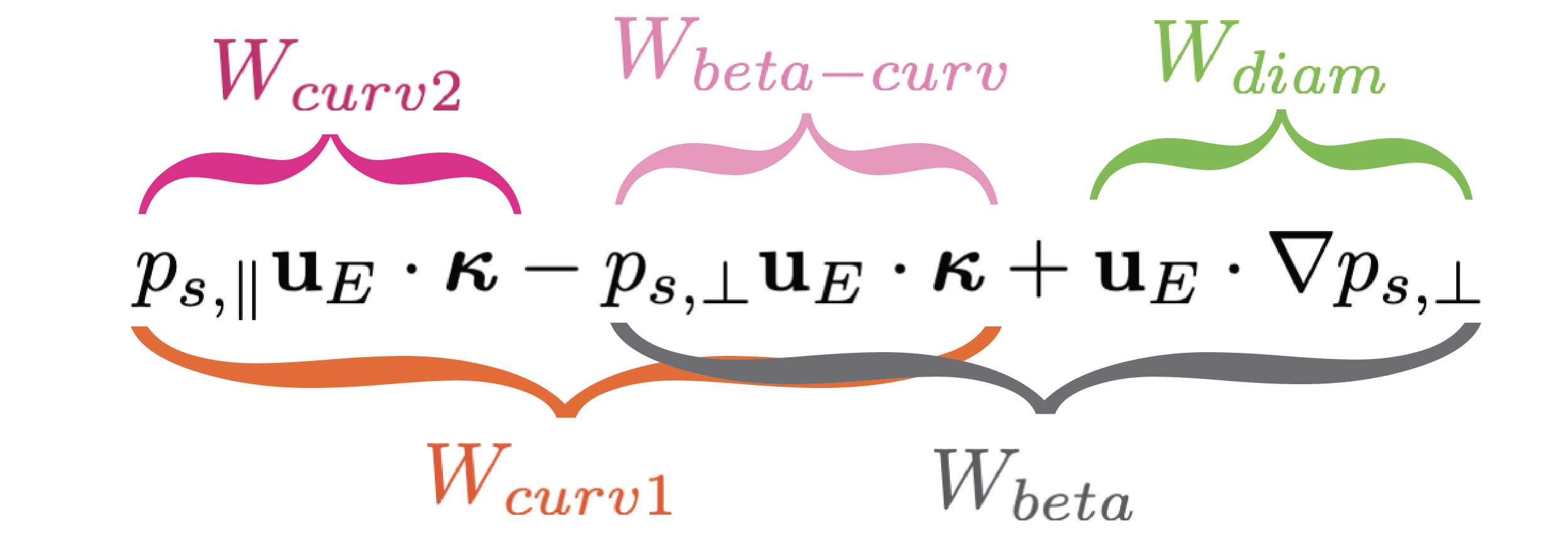
Motivated by the alternative guiding-center drift energization equation, Eq. (20), we can perform a final, alternative re-organization of the fluid-drift energization equation,
| (13) | |||||
This formulation separates the two curvature-related drift energization terms, which will make later comparison of the drifts more transparent.
To aid in following the three different groupings of the curvature, betatron, and diamagnetic drift terms, Fig. 1 provides a visual illustration of the groupings. The color-coding corresponds to that used in Fig. 4.
Finally, we note that the curvature term appearing in Eq. (4) is contained in the Eulerian polarization drift term, since
| (14) | |||||
where . We find below that contributes little to the electron energization. Since is small, this term is itself either small or mostly cancelled by other terms appearing in . Therefore, we do not separate it when discussing Eulerian energization.
III Simulation Setup
To study electron energization in magnetic reconnection, we employ the fully kinetic continuum Vlasov-Maxwell solver portion of the Gkeyll framework Juno et al. (2018); Hakim and Juno (2020). Gkeyll directly evolves the full Vlasov-Maxwell system in up to 3D-3V, three configuration and three velocity space dimensions, for an arbitrary number of species using the discontinuous Galerkin discretization scheme in all phase space dimensions.
To initialize magnetic reconnection, we follow the basic initial conditions of the Geospace Environment Modeling (GEM) reconnection challenge Birn et al. (2001). Therefore, we initialize a Harris sheet with the following magnetic field and density profiles:
| (15) |
| (16) |
with uniform ion and electron temperatures, and , satisfying . To maintain electron magnetization throughout the layer Swisdak et al. (2005), we add a uniform, moderate guide field, , to the above magnetic field profile. Pressure balance requires that , which implies . We choose , a reduced mass ratio, , and speed of light, , where is the in-plane, upstream, electron Alfvén speed. The layer thickness, , is taken to be , where is the ion inertial length. The simulation domain is chosen to be , , , where , , and the same velocity space extents are used in each species’ three velocity dimensions, except we extend the velocity space extents of the electrons in the guide field direction to to resolve additional particle acceleration. Periodic boundary conditions are employed in the direction and conducting (reflecting) walls for the fields (particles) are used in the direction, while we employ zero-flux boundary conditions in velocity space. configuration space cells and velocity space cells are used for the protons and electrons with piecewise quadratic Serendipity polynomial basis functions Arnold and Awanou (2011) to discretize the fields and particle distribution functions. We also employ a conservative Lenard-Bernstein collision operator Lenard and Bernstein (1958); Hakim et al. (2020) with electron-electron collision frequency and ion-ion collision frequency . The collision frequencies are chosen to satisfy the weakly collisional limit while being sufficient to regularize velocity space and maintain numerical stability.
To initiate reconnection, an initial magnetic flux function,
| (17) |
is specified with , where the perturbed magnetic field resulting from this flux is . To break the symmetry inherent to these initial conditions in a noise-free simulation, the first twenty and magnetic field modes are randomly perturbed with a root-mean-square amplitude .
IV Simulation Results
IV.1 Overall Evolution
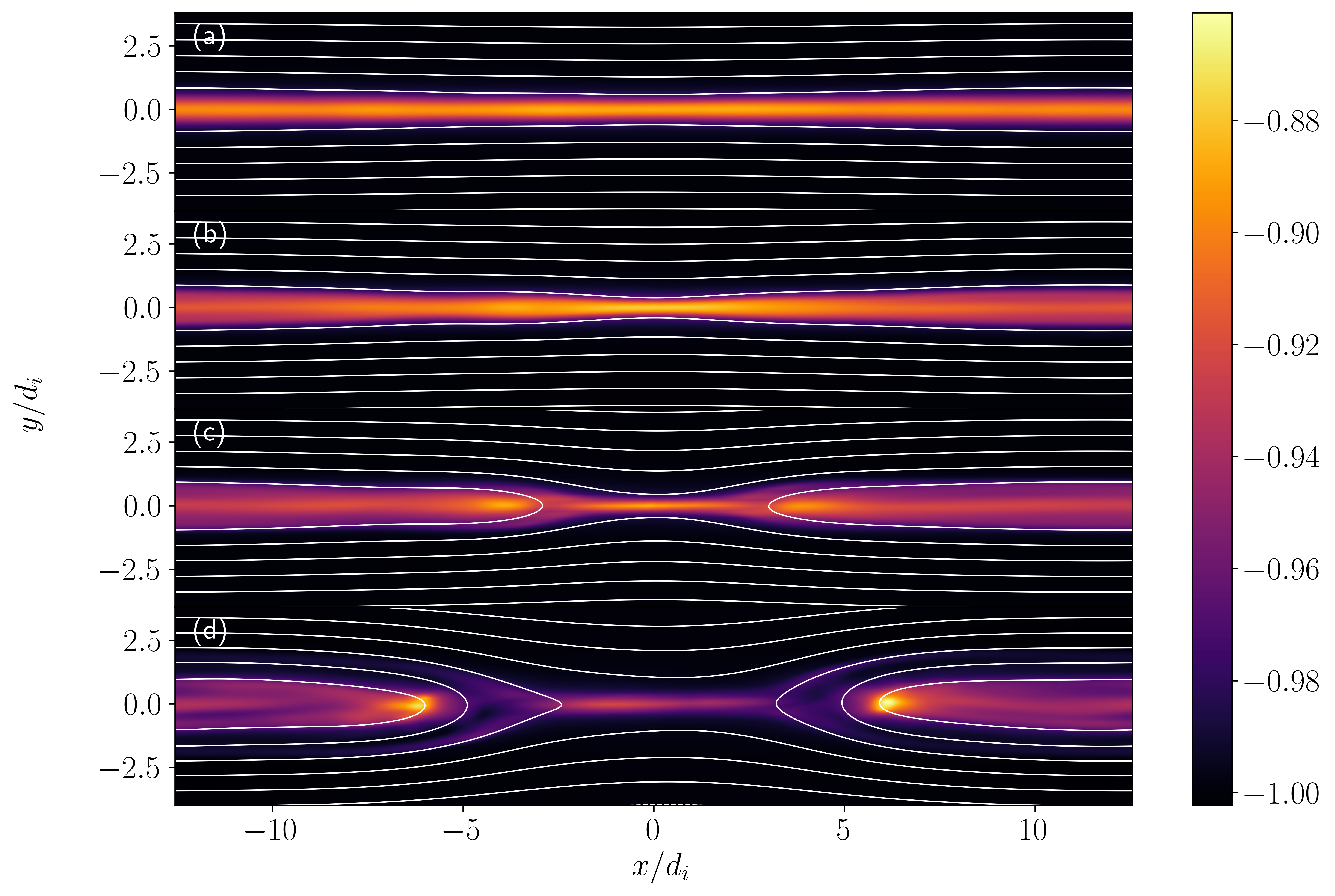
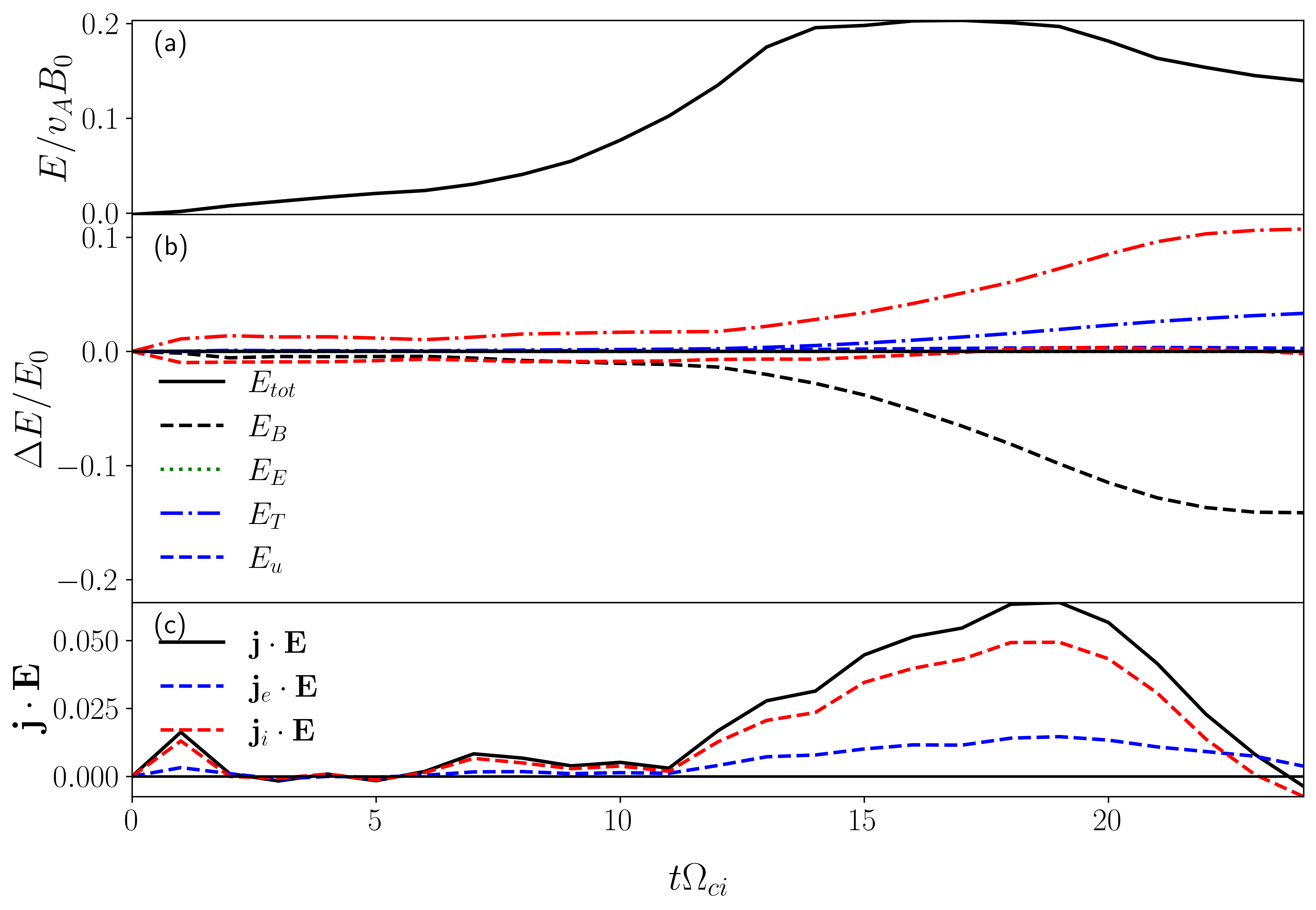
In Fig. 2, we present the evolution of the out-of-plane current density, , in color along with contours of the out-of-plane vector potential, , at and in panels (a)-(d), respectively. In Fig. 3, we present the reconnection rate (a), integrated and normalized change in energy components (b), and the work (c). The components of the spatially integrated and normalized change in energy in panel (b) are defined as: is the magnetic energy, is the electric field energy, is the flow energy, is the thermal energy, , , and . In panels (b) and (c), red (blue) lines correspond to ion (electron) quantities. From these panels, we can see that the electron work peaks at , shortly after the peak reconnection rate. We will focus on this time for our local analyses of electron energization.
IV.2 Electron Energization
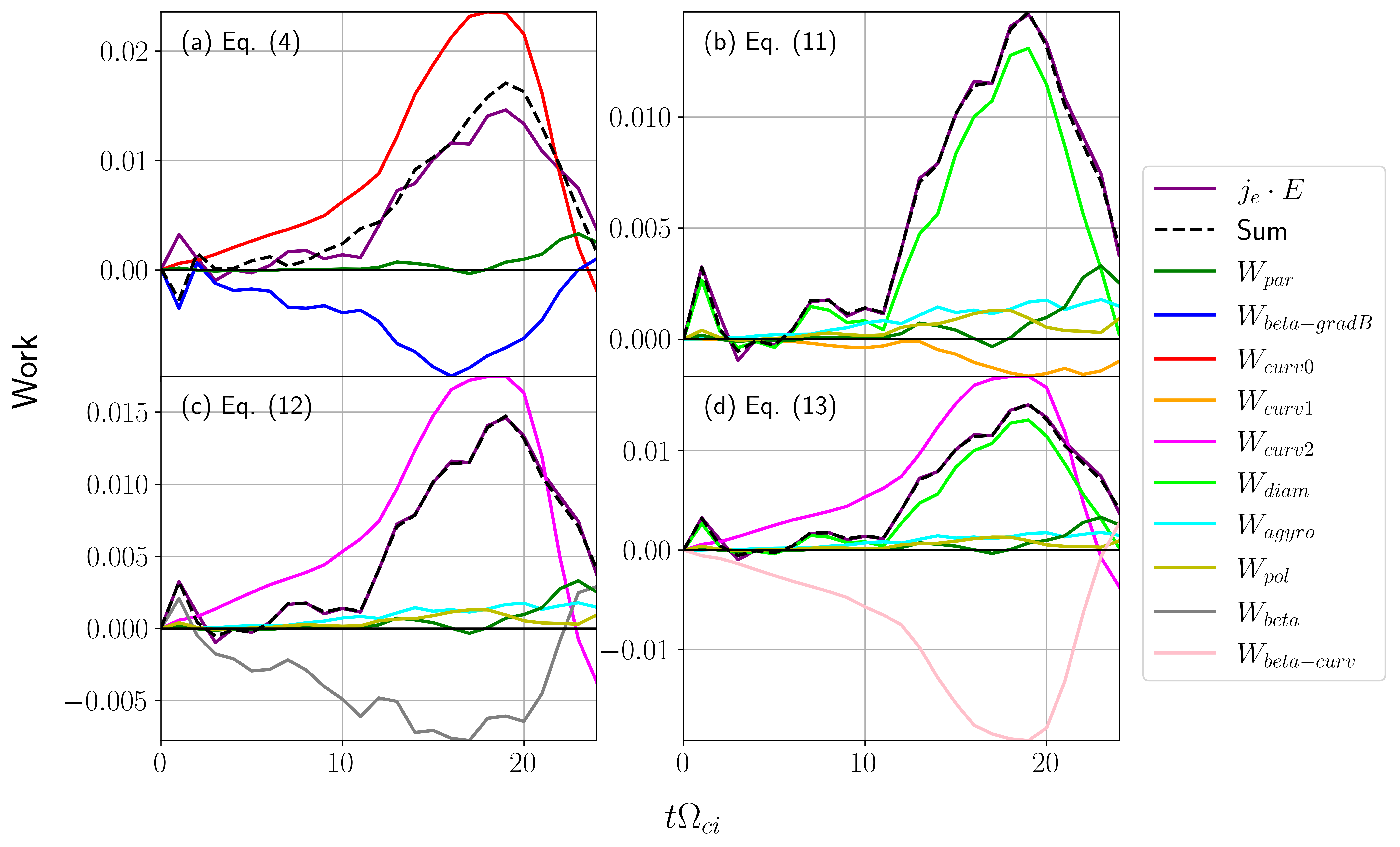
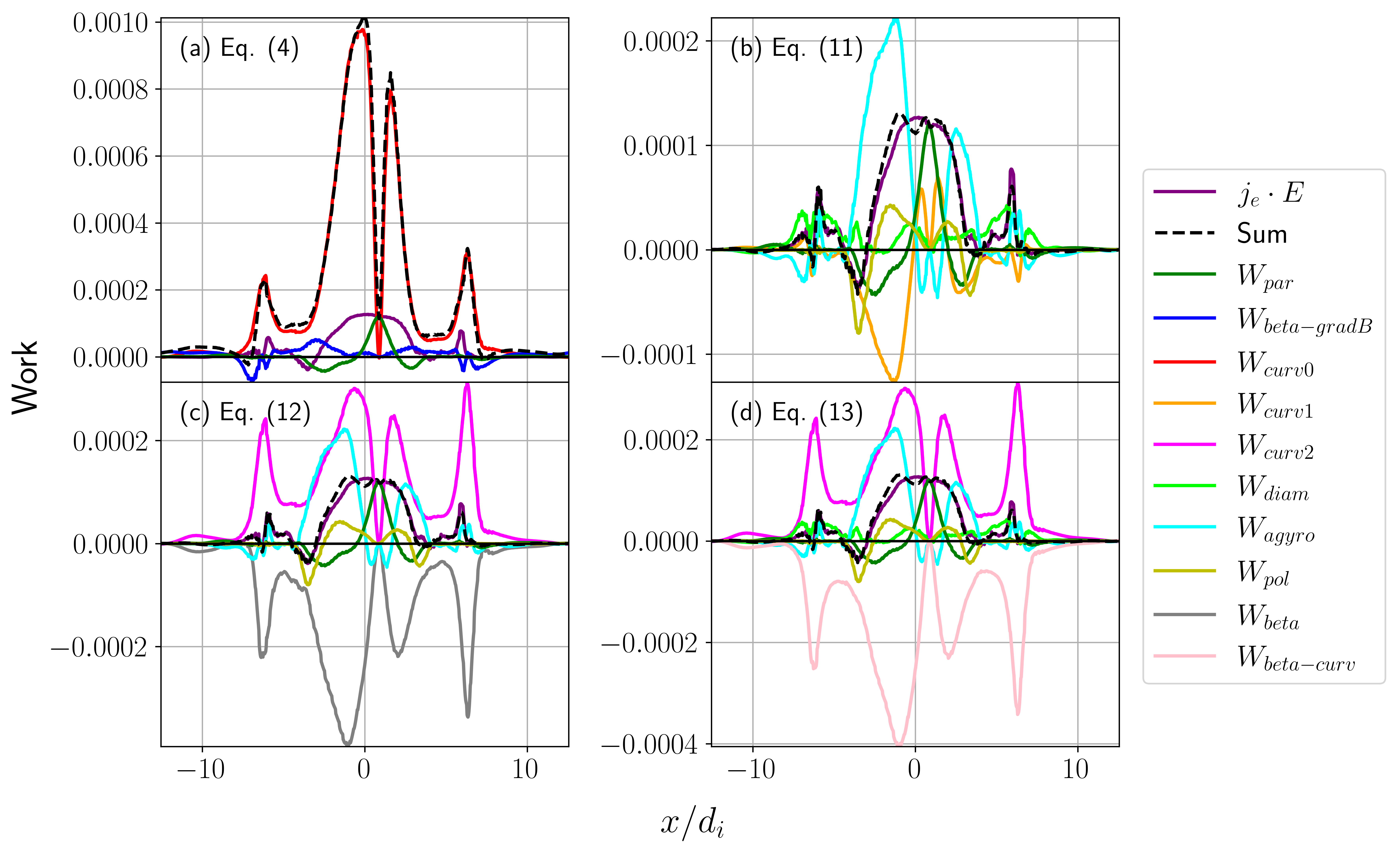
Following Dahlin et al. (2014); Li et al. (2015, 2017), we integrate over the entire domain to examine the drift energization terms and their sums in Eqs. 4, II.2, and II.2, which are plotted in Fig. 4. The guiding-center energization terms (Eq. (4)) plotted in panel (a) display the expected results based on PIC simulations: the curvature drift (red) is large, positive, and the primary contributor to the sum (dashed black); the (blue) is negative due to the conversion of magnetic energy into particle energy; and (green) is positive but small. However, the sum and the directly computed (magenta) track each other well but display quantitative differences of up to 20%, suggesting that non-negligible energization terms may be missing.
Moving to the Eulerian energization formulations in Eqs. II.2 and II.2 in panels (b) and (c) respectively, we first note that the sum (black dashed) and (purple) agree very well at all times, indicating that all significant energization is included, as expected for a rigorous accounting of all bulk flow motion. Next, we note that the diamagnetic drift (lime), , is the primary contributor to the domain integrated work in panel (b). For the base Eulerian energization formulation, Eq. (II.2), the curvature drift (orange), , is at all times negative in panel (b). The agyrotropic (cyan) and polarization (yellow) drifts as well as contribute little to the total. Mirroring the guiding-center formulation using Eq. (II.2) and splitting the curvature drift, , into parallel curvature drift, , (magenta) and betatron acceleration, , (grey) in panel (c), we now see that this form of the curvature drift is large and positive, dominating all other drifts, except at late times. In panel (d), we repeat the decomposition found in panel (b), except we separate the diamagnetic () and curvature-like betatron (pink), , terms (see Fig. 1 for a visual illustration of the groupings of curvature, betatron, and diamagnetic drifts). Here, we see clearly that the curvature-like betatron term (pink), , and (magenta) have similar magnitudes and opposite signs, with being larger for most of the simulation, leading to being small and negative in the panel (b).
To make the comparison between drift models and their terms more quantitative, Table 1 presents the same domain integrated values as Fig. 4 but focusing on . Each term of the different energization formulations is presented separately, normalized to , and the sum column entries refer to the sum of all contributing terms in that row. Here, we can see more clearly that the guiding-center formulation overestimates the energization by %, while the fluid energization approaches are equivalent and accurate to within %. We can also see that the diamagnetic drift contributes % of the overall energization. Finally, using Eq. (13), it is clear that and almost cancel each other, leaving a remainder of , an overall loss of energy due to the fluid curvature drift.
| Equation | Sum | |||||||||||
|---|---|---|---|---|---|---|---|---|---|---|---|---|
| [Eq. (4)] | 1 | 0.0484 | -0.4866 | 1.6062 | - | - | - | - | - | - | - | 1.1681 |
| [Eq. (II.2)] | 1 | 0.0484 | - | - | 0.8959 | -0.1144 | 0.1136 | 0.0644 | - | - | - | 1.0079 |
| [Eq. (II.2)] | 1 | 0.0484 | - | - | - | - | 0.1136 | 0.0644 | 1.1971 | -0.4157 | - | 1.0079 |
| [Eq. (13)] | 1 | 0.0484 | - | - | 0.8959 | - | 0.1136 | 0.0644 | 1.1971 | - | -1.3116 | 1.0079 |
Next, we look at cuts of the energization terms along the mid-plane at at the time of maximum energization (). In Fig. 5, we present these cuts using the same four drift formulations presented in Fig. 4. First, at the x-point, , all of the energization is due to the parallel acceleration term (green), . Using the guiding center formulation Eq. (4) (a), we see that away from the x-point, the curvature drift term is the largest contributor; however, we also see that the sum (dashed black) does not well agree with the directly computed at any point along the cut. Using the Eulerian description Eq. (II.2) (b), we see that the largest positive contributor is the agyrotropic drift (cyan), and the curvature drift (orange) is generally large and negative at the same position in . Using the alternative Eulerian description Eq. (II.2) (c), again the curvature drift (magenta) is generally large and positive but is mostly balanced by an even larger, negative contribution from the betatron term (grey). In panel (d), we again repeat the decomposition found in panel (b), except we separate the diamagnetic (lime) and curvature-like betatron terms (pink). In all cases, we note that at most points away from the x-point, several drifts contribute simultaneously with comparable amplitudes, with the agyrotropic drift generally dominating and the curvature drift () being generally negative.
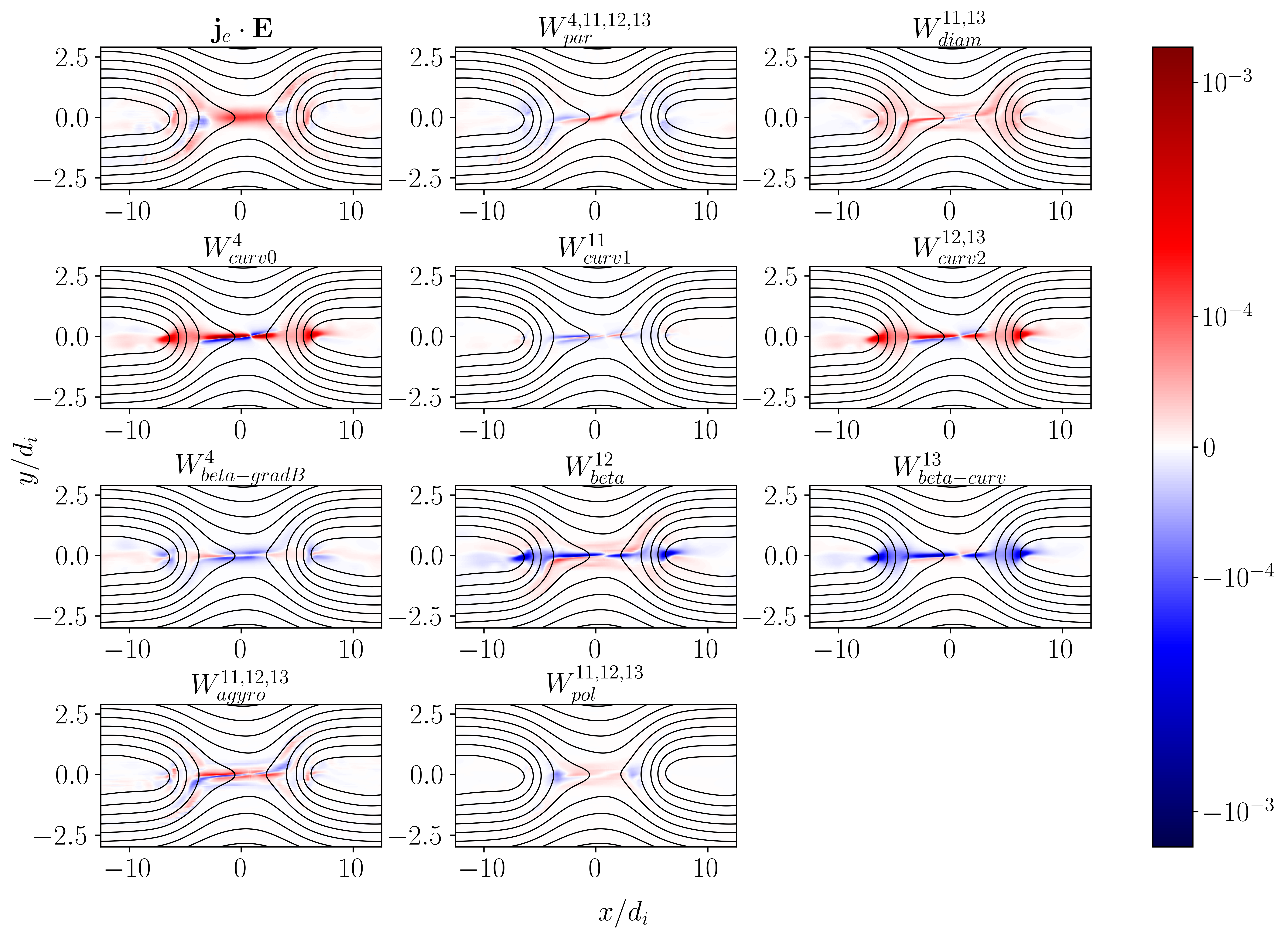
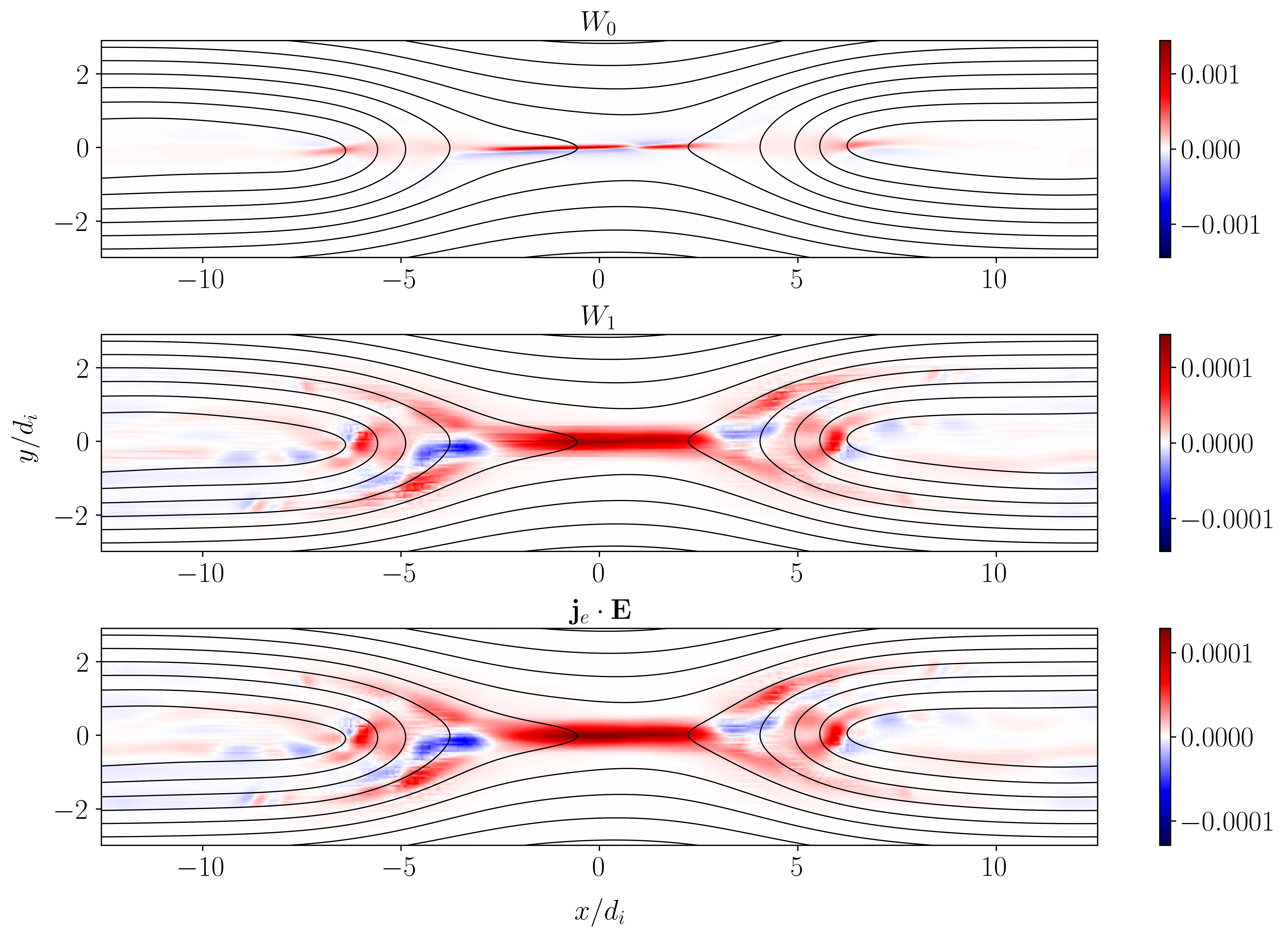
Finally, we examine the full spatial distribution of and its components at in Fig. 6 with black contours of the out-of-plane vector potential, , overplotted for reference. Superscript values indicate the drift energization equation in which the term appears. Due to the wide range of values, we employ a mixed log-linear color bar which is logarithmic for values and linear for values . From these panels, we can see: i) is large and positive in the vicinity of the x-point; ii) is mostly positive and is the most space-filling term; iii) is large and positive in the entire diffusion region; iv) is mostly negative; v) is the largest positive contributor in the downstream region and is generally negated by; vi) , which is the largest negative contributor, essentially cancelling everywhere. In Fig. 7, we present the sums of the guiding center drifts, , and the Eulerian drifts, in the top and middle panels. For comparison, we again plot . is entirely dominated by and does not follow the actual energization; whereas, is a nearly perfect match to the electron work.
V Discussion and Conclusions
The guiding-center description of electron energization, Eq. (4), clearly shows that curvature drift, , is the dominant energization mechanism in the reconnection simulation, both globally and locally, away from the x-point. However, neither globally nor locally does the sum of the energization mechanisms agree well with , suggesting that the Lagrangian description, unsurprisingly, does not work well in an Eulerian simulation. The disagreement can be partially ameliorated by including additional guiding-center drifts in Eq. (1), e.g., polarization, and properly transforming from guiding-centers to the fluid frame.
On the other hand, the Eulerian energization perspective, Eq. (II.2), is a rigorously complete description of all bulk-drift motion. This perspective suggests that the diamagnetic drift, , dominates globally with large local spikes of agyrotropic drift, , energization. We note that both of these drifts are unique to the Eulerian perspective and have no direct equivalent in a guiding-center model, even when summed over ensembles of guiding centers. Despite being rigorously complete, the nomenclature and grouping of drift terms in Eq. (II.2) is somewhat ambiguous, as demonstrated by the additional formulations in Eqs. II.2 and 13. We also note that the diamagnetic drift can be separated into and magnetization drifts, c.f., Appendix F of Juno et al. (2021).
In the Eulerian perspective, the curvature drift, , manifestly depends on the pressure anisotropy, differing significantly from the guiding-center description, which depends on only . The dependence on the pressure anisotropy leads to significant local and global cancellation, with and nearly cancelling each other everywhere in the domain. The strong negative correlation between the two components suggests that they should be combined as rather than separated. Although is generally negative in the simulation, clearly indicating that the curvature drift leads to a net loss of energy, that does not mean that high energy particles are not being produced in the Eulerian picture. Since the Eulerian perspective provides information about bulk energization, it is possible for to produce an electron power-law tail leading to a bulk drift while produces a greater loss of bulk flow energy from the core of the distribution, resulting in an overall loss of energy due to the curvature drift. Further, we note that in the pressure isotropic limit, the fluid curvature drift mostly vanishes—the component of the curvature drift proportional to that formally appears in the polarization drift remains in the pressure isotropic limit. Indeed, this cancellation of curvature-drift terms in a pressure isotropic fluid is even noted in Goldston and Rutherford’s textbook Goldston and Rutherford (1995).
The guiding-center formulation can be manipulated to more closely resemble the Eulerian description, including the appearance of the term in Eq. (20). However, this manipulation is not well motivated physically and obfuscates the relevant guiding-center physics by re-expressing betatron acceleration as a series of other terms. The re-expression of the betatron term does, however, serve to highlight the problematic nature of attempting to apply a guiding-center description to an Eulerian system, whether that Eulerian system is a simulation or the solar wind. Because Eqs. 4 and 20 are derived by summing over ensembles of guiding centers, fluid moments like pressure and bulk flow arise, which provides a false impression that these guiding-center descriptions can be connected directly to fluid-like bulk evolution of the plasma (Eqs. 4 and 20), but that is not simply the case. Terms like the diamagnetic drift and agyrotropic drift will always be absent from any formal derivation based on guiding-center motion since guiding-center (or even particle) descriptions cannot account for bulk effects. Further, the guiding-center energization equation, Eq. (1), includes only the motion (drift) of the guiding center plus an induction term () that is due to the electric field acting on the gyroperiod integrated motion of an electron, which is not the complete motion of the particle. The motion of the particle in the reference frame in which the guiding-center is at rest is not included in Eq. (1), but to connect to an Eulerian perspective, this motion must be included. When this motion is included Goldston and Rutherford (1995), one arrives at the Eulerian description described herein for terms like the curvature drift.
So, where does this leave us? Are the prior PIC results indicating that curvature drift leads to significant particle energization incorrect? The short answer is no, because the particle guiding centers are indeed energized (accelerated) by , meaning that where that term is positive and large, particle guiding centers are gaining significant energy. However, that is not the full story, because the analysis typically leading to that conclusion is incomplete and typically performed in an Eulerian framework by integrating over regions of particles—this fact applies to both PIC simulations and spacecraft data. In the Eulerian perspective, one must also include additional terms arising from the full particle motion, not just the guiding-center drift plus gyroperiod integrated motion as included in the guiding-center energization equation. When doing so, the full Eulerian curvature drift, , may indicate a very different scenario for the electrons. In the case of the simulation examined herein, is relatively small and negative, whereas is large, positive, and the dominant contribution to electron energization. Fundamentally, this contradiction arises because the Eulerian picture describes the generation of bulk flows rather than guiding-center acceleration described by Eq. (1). The confusion follows from attempting to directly relate guiding-center acceleration described by Eq. (1) to bulk quantities described by the guiding-center ensemble integrated Eq. (4). The guiding-center ensemble equations do not include the full particle motion, nor do they account for bulk plasma properties that lead to bulk drifts, e.g., diamagnetic and agyrotropic effects. Therefore, the guiding-center ensemble energization Eq. (4) can be useful for highlighting regions of the plasma in which electrons are being accelerated by the curvature drift, potentially leading to highly energetic electrons via Fermi acceleration Drake et al. (2006); Dahlin et al. (2015, 2017); however, the guiding-center ensemble energization does not necessarily indicate regions in which electron bulk flows are large nor where electron heating (thermal broadening of the electron distribution) may be occurring. On the other hand, the Eulerian framework (Eq. (II.2)) only indicates where electrons are being energized in a bulk sense (bulk flows and heating), since in the Eulerian picture, there is no conception of single-particle or guiding-center motion.
In summary, the guiding-center approach can provide insights into high-energy particles, while the Eulerian approach gives a more complete perspective on the bulk energization and heating of the plasma. The Eulerian picture does describe the production of high energy particles, but only in a bulk sense as power-law tails of the distribution function, which in terms of moments, also lead to bulk flows. The guiding-center description of heating is incomplete, while the Eulerian approach provides no information about individual particle energization to high energies. We thus encourage a greater awareness of the desired goals when applying these diagnostics to the analysis of spacecraft data and simulations so that the proper diagnostic and perspective is applied. Finally, we note that field-particle correlations, by highlighting the different regions of velocity space in which particles are energized, may help to bridge this gap between the Lagrangian and Eulerian pictures Juno et al. (2021).
Acknowledgements.
The authors thank Hui Li for helpful discussions. This research is part of the Frontera computing project at the Texas Advanced Computing Center. Frontera is made possible by National Science Foundation (NSF) award OAC-1818253. JMT was supported by the NSF under grant number AGS-1842638. GGH was supported by the NSF grant AGS-1842561. J. Juno was supported by the U.S. Department of Energy under Contract No. DE-AC02-09CH1146 via an LDRD grant. The development of Gkeyll was partly funded by the NSF-CSSI program, Award Number 2209471.Data Availability Statement
Gkeyll is open source and can be installed by following the instructions on the Gkeyll website (http://gkeyll. readthedocs.io). The input file for the Gkeyll simulation presented here is available in the following GitHub repository, https://github.com/ammarhakim/gkyl-paper-inp.
Appendix A Alternative Guiding Center Formulation
We begin by noting that the betatron, , term appearing in Eq. (1) corresponds to induction and is due to the electric field acting on an electron during over its gyroperiod, i.e., it is due to particle motion beyond simple guiding-center motion. We can take advantage of this fact and note that
| (18) | |||||
where we have used the fact that in the guiding-center limit, . Therefore, Eq. (4) can be expressed as
| (19) | |||||
. With this substitution, it is apparent that a curvature-related term, , was hidden within the betatron term. We also note that is a compressional term similar in form to that studied by Li et al. (2018). However, we further note that , which integrated over all space implies , assuming there is no net flux of thermal energy into or out of the domain. Therefore, in a spatially integrated sense, as often presented in guiding-center analyses, this compressional betatron-related term is related to the Eulerian diamagnetic drift energization. Thus, the electron guiding-center energization can be expressed approximately as
| (20) | |||||
References
- Drenkhahn and Spruit (2002) G. Drenkhahn and H. C. Spruit, Astron. Astrophys. 391, 1141 (2002), arXiv:astro-ph/0202387 [astro-ph] .
- Lin et al. (2003) R. P. Lin, S. Krucker, G. J. Hurford, D. M. Smith, H. S. Hudson, G. D. Holman, R. A. Schwartz, B. R. Dennis, G. H. Share, R. J. Murphy, A. G. Emslie, C. Johns-Krull, and N. Vilmer, Astrophys. J. Lett. 595, L69 (2003).
- Michel (1994) F. C. Michel, Astrophys. J. 431, 397 (1994).
- Krucker et al. (2010) S. Krucker, H. S. Hudson, L. Glesener, S. M. White, S. Masuda, J. P. Wuelser, and R. P. Lin, Astrophys. J. 714, 1108 (2010).
- Oka et al. (2013) M. Oka, S. Ishikawa, P. Saint-Hilaire, S. Krucker, and R. P. Lin, Astrophys. J. 764, 6 (2013), arXiv:1212.2579 [astro-ph.SR] .
- Drake et al. (2006) J. F. Drake, M. Swisdak, H. Che, and M. A. Shay, Nature 443, 553 (2006).
- Guo et al. (2014) F. Guo, H. Li, W. Daughton, and Y.-H. Liu, Phys. Rev. Lett. 113, 155005 (2014), arXiv:1405.4040 [astro-ph.HE] .
- Zhdankin et al. (2018) V. Zhdankin, D. A. Uzdensky, G. R. Werner, and M. C. Begelman, Astrophys. J. Lett. 867, L18 (2018), arXiv:1805.08754 [astro-ph.HE] .
- Comisso and Sironi (2018) L. Comisso and L. Sironi, Phys. Rev. Lett. 121, 255101 (2018), arXiv:1809.01168 [astro-ph.HE] .
- Parker (1983) E. N. Parker, Astrophys. J. 264, 642 (1983).
- Parker (1988) E. N. Parker, Astrophys. J. 330, 474 (1988).
- Drake and Swisdak (2012) J. F. Drake and M. Swisdak, Space Sci. Rev. 172, 227 (2012).
- TenBarge and Howes (2013) J. M. TenBarge and G. G. Howes, Astrophys. J. Lett. 771, L27 (2013), arXiv:1304.2958 [physics.plasm-ph] .
- Karimabadi et al. (2013) H. Karimabadi, V. Roytershteyn, M. Wan, W. H. Matthaeus, W. Daughton, P. Wu, M. Shay, B. Loring, J. Borovsky, E. Leonardis, S. C. Chapman, and T. K. M. Nakamura, Phys. Plasmas 20, 012303 (2013).
- Chasapis et al. (2017) A. Chasapis, W. H. Matthaeus, T. N. Parashar, O. Le Contel, A. Retinò, H. Breuillard, Y. Khotyaintsev, A. Vaivads, B. Lavraud, E. Eriksson, T. E. Moore, J. L. Burch, R. B. Torbert, P. A. Lindqvist, R. E. Ergun, G. Marklund, K. A. Goodrich, F. D. Wilder, M. Chutter, J. Needell, D. Rau, I. Dors, C. T. Russell, G. Le, W. Magnes, R. J. Strangeway, K. R. Bromund, H. K. Leinweber, F. Plaschke, D. Fischer, B. J. Anderson, C. J. Pollock, B. L. Giles, W. R. Paterson, J. Dorelli, D. J. Gershman, L. Avanov, and Y. Saito, Astrophys. J. 836, 247 (2017).
- Shay et al. (2018) M. A. Shay, C. C. Haggerty, W. H. Matthaeus, T. N. Parashar, M. Wan, and P. Wu, Phys. Plasmas 25, 012304 (2018).
- Escoubet et al. (1997) C. P. Escoubet, R. Schmidt, and M. L. Goldstein, Space Sci. Rev. 79, 11 (1997).
- Angelopoulos (2008) V. Angelopoulos, Space Sci. Rev. 141, 5 (2008).
- Burch et al. (2016a) J. L. Burch, T. E. Moore, R. B. Torbert, and B. L. Giles, Space Sci. Rev. 199, 5 (2016a).
- Phan et al. (2013) T. D. Phan, M. A. Shay, J. T. Gosling, M. Fujimoto, J. F. Drake, G. Paschmann, M. Oieroset, J. P. Eastwood, and V. Angelopoulos, Geophys. Res. Lett. 40, 4475 (2013).
- Burch et al. (2016b) J. L. Burch, R. B. Torbert, T. D. Phan, L.-J. Chen, T. E. Moore, R. E. Ergun, J. P. Eastwood, D. J. Gershman, P. A. Cassak, M. R. Argall, S. Wang, M. Hesse, C. J. Pollock, B. L. Giles, R. Nakamura, B. H. Mauk, S. A. Fuselier, C. T. Russell, R. J. Strangeway, J. F. Drake, M. A. Shay, Y. V. Khotyaintsev, P.-A. Lindqvist, G. Marklund, F. D. Wilder, D. T. Young, K. Torkar, J. Goldstein, J. C. Dorelli, L. A. Avanov, M. Oka, D. N. Baker, A. N. Jaynes, K. A. Goodrich, I. J. Cohen, D. L. Turner, J. F. Fennell, J. B. Blake, J. Clemmons, M. Goldman, D. Newman, S. M. Petrinec, K. J. Trattner, B. Lavraud, P. H. Reiff, W. Baumjohann, W. Magnes, M. Steller, W. Lewis, Y. Saito, V. Coffey, and M. Chandler, Science 352, aaf2939 (2016b).
- Chen et al. (2008) L. J. Chen, A. Bhattacharjee, P. A. Puhl-Quinn, H. Yang, N. Bessho, S. Imada, S. Mühlbachler, P. W. Daly, B. Lefebvre, Y. Khotyaintsev, A. Vaivads, A. Fazakerley, and E. Georgescu, Nature 4, 19 (2008).
- Sitnov et al. (2019) M. Sitnov, J. Birn, B. Ferdousi, E. Gordeev, Y. Khotyaintsev, V. Merkin, T. Motoba, A. Otto, E. Panov, P. Pritchett, F. Pucci, J. Raeder, A. Runov, V. Sergeev, M. Velli, and X. Zhou, Space Sci. Rev. 215, 31 (2019).
- Oka et al. (2022) M. Oka, T. Phan, M. Øieroset, D. Turner, J. Drake, X. Li, S. Fuselier, D. Gershman, B. Giles, R. Ergun, R. Torbert, H. Wei, R. Strangeway, C. Russell, and J. Burch, Phys. Plasmas 29, 052904 (2022).
- Øieroset et al. (2023) M. Øieroset, T. D. Phan, M. Oka, J. F. Drake, S. A. Fuselier, D. J. Gershman, K. Maheshwari, B. L. Giles, Q. Zhang, F. Guo, J. L. Burch, R. B. Torbert, and R. J. Strangeway, Astrophys. J. 954, 118 (2023).
- Dahlin et al. (2014) J. T. Dahlin, J. F. Drake, and M. Swisdak, Phys. Plasmas 21, 092304 (2014), arXiv:1406.0831 [physics.plasm-ph] .
- Dahlin et al. (2015) J. T. Dahlin, J. F. Drake, and M. Swisdak, Phys. Plasmas 22, 100704 (2015), arXiv:1503.02218 [physics.plasm-ph] .
- Dahlin et al. (2017) J. T. Dahlin, J. F. Drake, and M. Swisdak, Phys. Plasmas 24, 092110 (2017), arXiv:1706.00481 [physics.plasm-ph] .
- Li et al. (2015) X. Li, F. Guo, H. Li, and G. Li, Astrophys. J. Lett. 811, L24 (2015), arXiv:1505.02166 [astro-ph.SR] .
- Li et al. (2017) X. Li, F. Guo, H. Li, and G. Li, Astrophys. J. 843, 21 (2017).
- Dahlin et al. (2016) J. T. Dahlin, J. F. Drake, and M. Swisdak, Phys. Plasmas 23, 120704 (2016), https://doi.org/10.1063/1.4972082 .
- McCubbin et al. (2022) A. J. McCubbin, G. G. Howes, and J. M. TenBarge, Phys. Plasmas 29, 052105 (2022), arXiv:2112.06862 [physics.plasm-ph] .
- Northrop (1963) T. G. Northrop, The Adiabatic Motion of Charged Particles (Interscience Publishers, 1963).
- Parker (1957) E. N. Parker, Phys. Rev. 107, 924 (1957).
- Blandford et al. (2014) R. Blandford, P. Simeon, and Y. Yuan, Nuclear Physics B Proceedings Supplements 256, 9 (2014), arXiv:1409.2589 [astro-ph.HE] .
- Li et al. (2018) X. Li, F. Guo, H. Li, and J. Birn, Astrophys. J. 855, 80 (2018), arXiv:1801.02255 [physics.plasm-ph] .
- Beresnyak and Li (2016) A. Beresnyak and H. Li, Astrophys. J. 819, 90 (2016), arXiv:1406.6690 [astro-ph.HE] .
- Du et al. (2022) S. Du, H. Li, X. Fu, Z. Gan, and S. Li, Astrophys. J. 925, 128 (2022), arXiv:2112.02667 [physics.space-ph] .
- Klein and Howes (2016) K. G. Klein and G. G. Howes, Astrophys. J. Lett. 826, L30 (2016), arXiv:1607.01738 [physics.space-ph] .
- Howes et al. (2017) G. G. Howes, K. G. Klein, and T. C. Li, J. Plasma Phys. 83, 705830102 (2017).
- Klein et al. (2017) K. G. Klein, G. G. Howes, and J. M. Tenbarge, J. Plasma Phys. 83, 535830401 (2017), arXiv:1705.06385 [physics.plasm-ph] .
- Chen et al. (2019) C. H. K. Chen, K. G. Klein, and G. G. Howes, Nature 10, 740 (2019), arXiv:1902.05785 [physics.space-ph] .
- Klein et al. (2020) K. G. Klein, G. G. Howes, J. M. TenBarge, and F. Valentini, J. Plasma Phys. 86, 905860402 (2020), arXiv:2006.02563 [physics.plasm-ph] .
- Juno et al. (2021) J. Juno, G. G. Howes, J. M. TenBarge, L. B. Wilson III, A. Spitkovsky, D. Caprioli, K. G. Klein, and A. Hakim, J. Plasma Phys. 87, 905870316 (2021), arXiv:2011.13829 [physics.plasm-ph] .
- Juno et al. (2023) J. Juno, C. R. Brown, G. G. Howes, C. C. Haggerty, J. M. TenBarge, I. Wilson, Lynn B., D. Caprioli, and K. G. Klein, Astrophys. J. 944, 15 (2023), arXiv:2211.15340 [physics.plasm-ph] .
- Chew et al. (1956) G. L. Chew, M. L. Goldberger, and F. E. Low, "Proc. R. Soc. London A" 236, 112 (1956).
- Goldston and Rutherford (1995) R. J. Goldston and P. H. Rutherford, Introduction to Plasma Physics (Institute of Physics Publishing, 1995).
- Juno et al. (2018) J. Juno, A. Hakim, J. TenBarge, E. Shi, and W. Dorland, Journal of Computational Physics 353, 110 (2018), arXiv:1705.05407 [physics.plasm-ph] .
- Hakim and Juno (2020) A. Hakim and J. Juno, in Proceedings of the International Conference for High Performance Computing, Networking, Storage and Analysis (IEEE Press, 2020).
- Birn et al. (2001) J. Birn, J. F. Drake, M. A. Shay, B. N. Rogers, R. E. Denton, M. Hesse, M. Kuznetsova, Z. W. Ma, A. Bhattacharjee, A. Otto, and P. L. Pritchett, J. Geophys. Res. 106, 3715 (2001).
- Swisdak et al. (2005) M. Swisdak, J. F. Drake, M. A. Shay, and J. G. McIlhargey, J. Geophys. Res. 110, A05210 (2005), physics/0503064 .
- Arnold and Awanou (2011) D. N. Arnold and G. Awanou, Foundations of Comp. Math 11, 337 (2011).
- Lenard and Bernstein (1958) A. Lenard and I. B. Bernstein, Phys. Rev. 112, 1456 (1958).
- Hakim et al. (2020) A. Hakim, M. Francisquez, J. Juno, and G. W. Hammett, J. Plasma Phys. 86, 905860403 (2020), arXiv:1903.08062 [physics.comp-ph] .