Soft supersymmetry breaking as the sole origin of neutrino masses and lepton number violation
Abstract
We discuss a scenario in which the supergravity induced soft terms, conventionally used for breaking supersymmetry, also lead to non-zero Majorana neutrino masses. The soft terms lead to the spontaneous violation of the lepton number at the gravitino mass scale which in turn leads to (i) the Majorana masses of for the right-handed neutrinos and (ii) the -parity breaking at the same scale. The former contributes to light neutrino masses through the type I seesaw mechanism, while the latter adds to it through neutrino-neutralino mixing. Both contributions can scale inversely with respect to given that gaugino and Higgsino masses are also of order . Together, these two contributions adequately explain observed neutrino masses and mixing. One realization of the scenario also naturally leads to a parameter of . Despite the lepton number symmetry breaking close to the weak scale, the Majoron in the model exhibits very weak coupling to leptons, satisfying existing constraints on Majoron-lepton interactions. The right-handed neutrinos in the model have a large coupling to Higgsinos. This coupling and the relatively large heavy-light neutrino mixing induced through the seesaw mechanism may lead to the observable signals at colliders in terms of displaced vertices.
I Introduction
Violation of the lepton number, which otherwise is an automatic classical symmetry of the standard model (SM), provides an appealing avenue to account for small but non-vanishing neutrino masses Weinberg (1979). It enables neutrinos to become Majorona particles and associates their masses to a new scale in the theory. The exact relation between the neutrino mass scale and a new scale depends on the nature of new physics introduced to violate the lepton number (LN) Mohapatra et al. (2007). For example, the most popular among these is the type I seesaw mechanism Minkowski (1977); Yanagida (1979); Mohapatra and Senjanovic (1980); Schechter and Valle (1980) in which two or more right-handed (RH) neutrinos are introduced and coupled to the SM neutrinos through Yukawa interactions. A Majorana mass of RH neutrino denotes the scale of LN violation in this case. It can be put in by hand or may arise from the spontaneous breaking of a gauge symmetry that includes the LN Fritzsch and Minkowski (1975); Gell-Mann et al. (1979). From the perspective of the light neutrino masses, the RH neutrino mass scale can be as high as GeV if they strongly couple to the SM. On the other hand, can be as light as of the order of the electroweak scale provided that their couplings with the SM leptons are small.
The other compelling reason to extend the SM comes from the gauge hierarchy problem. The electroweak scale can be stabilised in the presence of some large scale in the theory when the SM is supersymmetrised by replacing it with the minimal supersymmetric standard model (MSSM), see Martin (1998) for a comprehensive review. An efficient implementation of this scheme requires the mass scale of the MSSM fields not very different from the electroweak scale. The existence of all Dimopoulos and Georgi (1981); Dimopoulos et al. (1981); Marciano and Senjanovic (1982) or at least some Arkani-Hamed and Dimopoulos (2005); Giudice and Romanino (2004) of the super-partners around the TeV scale also improves the unification of gauge couplings. Theoretically, the mass scale of the MSSM is set by the parameter and the soft supersymmetry (SUSY) breaking scale. The latter is linked to the mass of the gravitino in theories based on supergravity (see Lahanas and Nanopoulos (1987) for a review). Like in the case of SM, the MSSM can also be extended to incorporate LN violation as both are independent extensions of the SM. In this case, the scale of LN violation can coexist in the theory independent of and .
This paper aims to point out an interesting scenario in which the soft terms generated in supergravity theory not only break the SUSY but also spontaneously break the LN thereby linking the LN violation scale to the gravitino mass . The amalgamation of the otherwise two distinct scales provides a compelling reason to expect a low-scale LN violation if the SUSY is to resolve the gauge hierarchy problem or it is responsible for the precision unification of the strong and electroweak forces. Soft SUSY breaking terms proportional to exclusively generate Majorana masses for both the RH and the light neutrinos. The masses of the first are while those of the latter are induced through the seesaw mechanism. We propose a concrete and minimal realisation of the above scenario in this paper. This minimal version is shown to be complete in the sense that it leads to a consistent and predictive description of the neutrino masses and mixing.
It is noteworthy that connections between the mass of RH neutrino(s) and the SUSY breaking scale can also be established through different mechanisms. In the model known as MSSM Lopez-Fogliani and Munoz (2006); Escudero et al. (2008); Ghosh and Roy (2009); Fidalgo et al. (2009); Lopez-Fogliani and Munoz (2020), the RH neutrino masses arise through the most general trilinear terms in the superpotential when their superpartners acquire non-vanishing vacuum. The later is linked to the electroweak symmetry breaking scale which is indirectly related to the SUSY breaking through its radiative induction Ibanez and Ross (1982). The LN symmetry is explicitly violated in this model and, therefore, the Dirac and RH neutrino mass terms take the most general form. In another approach Chun et al. (1995, 1996); Chun (1999); Choi et al. (2001); Lavignac and Medina (2021); Joshipura and Patel (2021), LN is spontaneously broken but it’s scale is independent of the SUSY breaking scale. However, one of the RH neutrinos is arranged to be a fermionic partner of the Goldstone boson of the global LN symmetry and, therefore, this pair remains massless at the scale of LN violation. Subsequently, the fermionic partner gets a mass of when SUSY is broken through supergravity. Even though there is no in-principle connection between the LN breaking scale and in this kind of setup, the viable neutrino masses in the simplest versions of this framework force these two scales to stay close to each other Joshipura and Patel (2021). In the framework we propose here, these two scales are inherently and directly interlinked. This connection, along with the presence if LN symmetry in the full theory, is shown to lead to a realistic and more predictive setup for the neutrino masses compared to previous approaches.
The remainder of the paper is organised as follows. We discuss the basic mechanism leading to a connection between the SUSY breaking and LN violation in the next section. A comprehensive analysis of the light neutrino masses and mixing is presented in section III. We compute the couplings of Majoron with the light neutrinos and charged leptons in sections IV and V, respectively, and discuss the phenomenological constraints. In section VI, we discuss the RH neutrino mass spectrum and the possibility of probing them in direct search experiments. The study is concluded in section VII.
II Lepton number violation from soft SUSY breaking
In the following, we discuss two different types of frameworks. Both lead to violation of the LN through soft SUSY breaking. However, they are characteristically different in their implication for the neutrino masses. The first scenario assumes a conformal superpotential without any mass scale and the other scenario allows for an explicit parameter.
II.1 Conformal
We consider the MSSM extended by three RH neutrino superfields , (). To achieve the required scenario, we demand that the superpotential is conformal, i.e. it does not contain any mass scales. This can be done for example by imposing an symmetry on under which all the chiral superfields carry charge . This leads to only cubic terms in . All the standard terms present in the MSSM superpotential, except for the term, are allowed in this case. The superpotential for the RH neutrinos is completely fixed by imposing an additional global LN-like symmetry under which carry charges . This leads to the following most general superpotential:
| (1) |
Couplings between the MSSM sector and also get restricted by the LN symmetry under which the leptonic doublets carry charge . These are given by
| (2) |
where are the weak singlet charged lepton superfields with lepton number . The couplings between and are chosen flavour diagonal without loss of generality.
Eqs. (1,2) admit a supersymmetric minimum in which scalar components of all the superfields have a vanishing minimum. All fermions including , are massless in this limit. These masses are induced by the soft breaking of SUSY. We introduce the following soft terms corresponding to :
| (3) |
where denotes a Lorentz scalar component of a superfield . The neutrino mass generation through these soft SUSY-breaking terms proceeds as follows. Minimization of the scalar potential with these soft terms leads to non-zero vacuum expectation values (VEVs) for . These generate the RH neutrino masses which in turn lead to the masses for the left-handed neutrinos through the weak scale type I seesaw mechanism. The non-zero VEVs also spontaneously break -parity along with the LN, generating additional R-violating contributions to the light neutrino masses. Both these contributions together describe the observed neutrino masses and mixing. We discuss some of the salient features of this neutrino mass generation here and differ the detailed discussion to the next section.
Minimisation of the scalar potential derived from and is carried out and discussed in Appendix A. It leads to the following VEVs:
| (4) |
where and are dimensionless parameters determined in general by , and the soft parameters. The equality in the VEVs of and follows from an assumption which makes the full scalar potential invariant under the interchange of and . In absence of such an assumption, one finds but with a constraint, . It is noteworthy that all three sneutrinos obtain VEV of the order of the gravitino mass. In this way, the scale of the LN violation is linked to the SUSY breaking scale.
Notably, the also generates the parameter as in the NMSSM Ellwanger et al. (2010). But unlike in the NMSSM now the magnitude of is also naturally tied to the gravitino mass:
| (5) |
The VEV also breaks spontaneously the -parity Masiero and Valle (1990); Barbier et al. (2005) and generates the bilinear R-violation from Eq. (2), described by three parameters:
| (6) |
The RH neutrino mass matrix following from Eqs. (1) and (4) is given, in the basis , by
| (7) |
where . This leads to the three RH neutrino masses as
| (8) |
where
| (9) |
One also finds
| (10) |
The geometrical mean of three RH neutrino masses is given by . Typically, when all the three RH neutrinos have masses of . implies one or more RH neutrinos with a mass smaller than .
The above together with the Dirac mass matrix following from Eq. (2) leads to the seesaw contribution to the light neutrino masses as
| (11) |
where
| (12) |
The neutrino masses are determined by the Dirac neutrino Yukawa couplings and the inverse of . Small (high) values of the former (latter) can result in the required suppression in the neutrino masses as it happens in the usual seesaw case. The neutrino mass thus would be automatically suppressed in models with high-scale SUSY breaking.
Interestingly, Eqs. (11,12) offer an alternative way of lowering the seesaw contribution to neutrino masses even in low-scale SUSY models. This can be done if the parameter in Eq. (1) is taken very small111This can be done in a technically natural way since the limit increases the symmetry of .. This breaks LN at a scale higher than , see Eq. (4), and results in a small . This way of suppressing neutrino masses can be interpreted in terms of the inverse seesaw mechanism often used for suppressing neutrino masses in the weak or TeV scale seesaw models Mohapatra and Valle (1986); Mohapatra (1986); Nandi and Sarkar (1986). It follows from Eq. (II.1) that one of the RH neutrinos, namely , becomes heavier compared to the other two if .
Integrating out results in a mass matrix, written in the basis ,
| (13) |
where and is matrix of the Yukawa couplings multiplied by the Higgs VEV . The matrix has a form typically used in the inverse seesaw with
| (14) |
representing the small LN breaking parameter suppressed by . For , Eq. (13) leads to the light neutrino mass matrix
| (15) |
which coincides with the seesaw result, Eq. (11), for .
It follows from Eq. (2) that only one combination of the neutrino fields couples to and obtains its mass through the canonical seesaw mechanism. An independent linear combination of the neutrino fields obtains its mass from the -parity violation induced by the soft terms. The -violation is characterised by given in Eq. (6). They give rise to the VEV for the left-handed sneutrino leading to the mixing of neutrinos with neutralinos. This mixing generates mass for the other combination of neutrinos. The -parity violating parameters increase with the gravitino mass. So naively, one would expect that this contribution to the neutrino masses would increase with in contrast to the seesaw contribution. However, this does not happen and both contributions can be inversely proportional to in a typical situation as we show below.
The -parity violating contribution is specified in the rotated basis in which bilinear -parity violation is rotated away from the superpotential Joshipura et al. (2002). These unprimed bases are defined as
| (16) |
where and are the original fields present in the superpotential Eq. (2). The -parity violating light neutrino mass matrix is obtained as (see the next section for the derivation)
| (17) |
with
| (18) |
Here are gaugino masses and are the VEVs of the Higgs fields .
In Eq. (17), denote the VEVs of the scalar superpartners of the electrically neutral component of . They are determined in terms of the soft parameters by minimising the relevant scalar potential. Writing
| (19) |
we find in this case
| (20) |
where . The details of the derivation of the above can be found in Appendix B. If one assumes universal boundary conditions at a high scale then the differences in soft parameters appearing in are generated at the low scale through renormalization effects and are small. In particular, the first term which gives a dominant contribution to is typically given by
| (21) |
Here, is the bottom quark Yukawa coupling and is the scale where the universality of the soft terms is imposed.
It is useful to eliminate Yukawa couplings and consider the ratio of the contributions and . We find
| (22) |
Following Eqs. (20,21), can be approximated as
| (23) |
This implies
| (24) |
Since is related to the two non-zero neutrino masses, it cannot be too small or large. The detailed fit to neutrino masses and mixing presented in the next section show that the magnitude of is of order unity. Requiring has implications for the allowed and the SUSY spectrum. Considering , we note that:
-
•
If gaugino masses and the parameter are similar to then is independent of since is inversely proportional to the gaugino masses. This implies that like the seesaw contribution, the -parity violating contribution to the neutrino masses is also inversely proportional to . Therefore, the neutrino masses can be suppressed without requiring too small Yukawa couplings as in the high-scale seesaw models. This scenario would conflict with the gauge coupling unification which requires gauginos at the electroweak scale.
-
•
If is held fixed around electroweak scale by choosing appropriately and the gaugino masses are also assumed to be of the order of () then the is proportional to (). Then the requirement, , implies an upper bound on . We will explore this point more quantitatively in the next section.
-
•
cannot be arbitrarily small and can be around if parameter and the gaugino masses are similar to . Thus, can provide only a mild suppression in the neutrino masses through inverse seesaw.
Some of the above features change when is not conformal and contains an independent scale as a bare term. We discuss this below.
II.2 with a bare -term
An explicit parameter can exist if symmetry used to obtain cubic potential is not insisted upon. This has a significant effect on neutrino masses which we now discuss. Consider the same superpotential with an added bare -term, namely
| (25) |
The effective parameter is now obtained as
| (26) |
We can altogether omit the -dependent term. In this case, is not tied to the gravitino mass and represents an independent scale. This can be technically done by imposing a discrete symmetry under which , and with .
The term leads to an additional soft term in the scalar potential. The of Eq. (20) is now replaced by a more general expression
| (27) |
The above is obtained using Eq. (144) derived explicitly in Appendix B. Unlike in the previous case, is non-zero even at a high scale since generally and parameters are not equal in supergravity-induced soft terms. The last term, therefore, dominates in Eq. (27). This increases the -parity violating contribution by a factor of around . Since the last term in dominates,
| (28) |
The ratio defined in Eq. (22) is now given by
| (29) |
This suggests that cannot be chosen small ruling out the possibility of an inverse seesaw mechanism entirely in this case. Also since is inversely proportional to the gaugino mass, one requires this mass to be and to have of order one.
We have neglected in the above discussions one more contribution to the light neutrino masses which arise from the mixing of the RH neutrinos with Higgsino originating from Eq. (2). This gives a much smaller contribution compared to the ones already discussed. Inclusion of this requires consideration of the full mass matrix of neutral fermions in the model which we discuss in the following section.
III Light neutrino masses and mixing
The model has 10 neutral fermions denoted as . The RH VEVs generated through soft terms cause mixing among them as mentioned in the earlier section. The full mixing generated by the superpotential in Eq. (25) and gauge interactions can be written as:
| (30) |
where is a matrix parametrized as
| (31) |
Here,
| (38) |
The is already given in Eq. (7) while
| (46) |
is the standard neutralino mass matrix of the MSSM Martin (1998). parity-violating couplings mix the neutralinos with the SM neutrinos. This mixing is denoted as . Specifically, Higgsino-neutrino mixing is given by and gaugino mixing is determined by the sneutrino VEVs . denotes the mixing of the singlet states with neutralinos following from Eq. (25). represents invariant Dirac mass term between neutrinos and singlet states. The above describes the general case with explicit term present. The conformal case is obtained by putting in appearing in .
III.1 Analytical form of effective neutrino mass matrix
The tree-level light neutrino mass matrix can be obtained from Eq. (31) in the seesaw approximation as
| (47) |
where and is the lower-right block of the full matrix given in Eq. (31). Neglecting term in and performing some algebraic simplification, we get
| (48) |
Here,
| (49) |
with
| (50) |
and
| (51) |
is determinant of matrix with
| (52) |
Substituting Eq. (51) in Eq. (49) and using Eq. (12), we find
| (53) |
Since for , the denominator provides only a small correction to the equality, .
The matrices in Eq. (48) are obtained as
| (54) |
| (55) |
In the above,
| (56) |
denote the VEVs of sneutrino in the basis in which the bilinear term is rotated away from the superpotential, see Eq. (II.1). Finally, the dimensionless coefficients in Eq. (48) are obtained as
| (57) |
and is defined in Eq. (18).
The structures of the first two terms in Eq. (48) coincide with the seesaw and parity violating terms obtained in the earlier section. The last term is generated by the mixing among the RH neutrino and Higgsino coming from Eq. (25). This mixing also modifies the overall coefficients of the seesaw and -violating interactions compared to the simplified case considered earlier. Using , the neutrino mass matrix can be further simplified to the following form
| (58) |
where we have define , and . The parameters are given by Eqs. (20) or Eq. (27) depending on the choice of -term in the model. Also,
| (59) |
Here, and are defined in Eqs. (12,22), respectively. denotes the overall scale of the seesaw contribution. The corresponds to the ratio of the -parity violating and seesaw terms. and respectively reduce to and of the earalier section when . In the following, we shall only be working with the tree-level neutrino mass matrix and will neglect the other sub-dominant radiative contributions. These include corrections to the seesaw mass matrix Grimus and Löschner (2018) and corrections generated by the effective trilinear R parity violating terms present in the rotated basis Barbier et al. (2005). The tree-level mass matrix considered here is by itself sufficient to reproduce the neutrino mass spectrum and the radiative corrections are not expected to change the results significantly.
The determinant of is vanishing. It predicts a massless neutrino. The eigenvector corresponding to the massless state can be determined using . This gives
| (60) |
In the diagonal basis of the charged leptons, the above is identified with the first (third) column of the leptonic mixing matrix for normal (inverted) hierarchy in the neutrino masses. The observed neutrino mixing angles then necessarily require , as well as . This requires sizeable flavour violations in the soft terms, a feature which was noticed also earlier in Joshipura et al. (2002); Romao et al. (2000); Hirsch et al. (2000) in the context of different frameworks.
III.2 Example solutions
We now demonstrate that the effective neutrino mass matrix, as obtained in Eq. (58), can account for the realistic neutrino masses and mixing observables. As mentioned earlier, the charged lepton Yukawa couplings can be chosen real and diagonal without loss of generality. Moreover, the parameters , , and appearing in the superpotential can be made real through redefinitions of various superfields. This along with an assumption for the real VEVs of and lead to real , and in Eq. (58). The phase of is also unphysical. Altogether, these six real parameters and complex are required to reproduce the realistic values of six observables, namely the solar and atmospheric neutrino masses, three mixing angles and the Dirac CP phase.
| Parameters | NH1 | NH2 | NH3 | NH4 |
|---|---|---|---|---|
| [eV] | 1.0 | 1.0 | 0.01 | 0.01 |
| -0.9831 | 1.0216 | -2.6937 | -1.7155 | |
| 0 | -0.9983 | 0 | -0.4891 | |
| 0.0782 | -0.1196 | 1.387 | -1.3511 | |
| -0.5964 | 0.9562 | -3.2619 | 3.1967 | |
| 1.1216 | 0.5015 | 0.5859 | 0.501 | |
| 0.971 | 0.8866 | 0.6797 | 0.6163 | |
| Parameters | NH5 | NH6 | NH7 | NH8 |
| [eV] | 1.0 | 1.0 | 0.01 | 0.01 |
| 0.9841 | 0.5857 | 2.704 | 1.8462 | |
| -3.1349 | -0.01 | -3.096 | -3.0176 | |
| 0 | -0.7847 | 0 | -0.4372 | |
| -0.0814 | 0.1684 | 1.3628 | -1.3123 | |
| -0.6049 | -0.4458 | 3.2386 | -3.1601 | |
| 1.1158 | 1.3175 | 0.5813 | 0.5004 | |
| 0.9714 | 0.7802 | 0.678 | 0.6197 |
| Parameters | IH1 | IH2 | IH3 | IH4 |
|---|---|---|---|---|
| [eV] | 1.0 | 1.0 | 0.01 | 0.01 |
| -0.982 | -0.5409 | -0.4514 | -0.347 | |
| 0 | -0.2272 | 0 | -0.1066 | |
| -0.2517 | -0.2393 | -11.2255 | 14.6181 | |
| -0.9077 | 0.8048 | 3.0287 | 3.7629 | |
| 1.1493 | 1.2026 | 1.5 | 1.4252 | |
| 1.0082 | 0.9881 | 1.3626 | 1.3282 | |
| Parameters | IH5 | IH6 | IH7 | IH8 |
| [eV] | 1.0 | 1.0 | 0.01 | 0.01 |
| 0.9826 | 0.0836 | 3.0314 | 2.8087 | |
| -3.1412 | -0.0039 | -3.1386 | -3.1384 | |
| 0 | -0.5321 | 0 | -0.0918 | |
| -0.5623 | -0.6534 | 4.3557 | 4.4436 | |
| -0.743 | 0.725 | -1.7175 | 1.735 | |
| 1.0669 | 1.1278 | 0.5083 | 0.5 | |
| 0.99 | 0.9772 | 0.7529 | 0.7463 |
Following the usual optimization technique Joshipura and Patel (2021), we find several example solutions for the parameters in which lead to the viable neutrino spectrum. First, we consider real which leads to the vanishing CP phase, . The latter is not directly observed and the present fits to the neutrino oscillation data Capozzi et al. (2017); de Salas et al. (2021); Esteban et al. (2020) allows within . We find solutions for two example values of and also consider a possibility in which the parameter can be zero. The solutions obtained in this way are displayed as the first four solutions in Table 1 (2) for normal (inverted) hierarchy in the neutrino masses. Subsequently, we also consider complex to account for the Dirac CP phase. These solutions are listed as NH5 to NH8 in the case of normal and IH5 to IH8 in the case of inverted hierarchy in the respective tables. All the NH (IH) solutions give , (), , () and (). Solutions with complex give () for the NH (IH) case. All these values correspond to the central values as obtained by the latest fit to the neutrino oscillation data (see, NuFIT 5.2) in Esteban et al. (2020).
The noteworthy feature of these fits is that implying that the scales associated with both the -violating contribution and the seesaw terms are similar in magnitudes. This can be used to draw important conclusions on the basic parameters of the model. The exact expression of , using Eqs. (III.1,10), can be rewritten as
| (61) |
Scenarios in which the common gaugino mass scale, , is arranged to stay close to the electroweak scale and , then leads to
| (62) |
While deriving the above, we have used the expression Eq. (28) for the parameter. The fact that the value of cannot be arbitrarily large, as indicated by the fits, implies that the gaugino mass scale cannot be much smaller than if . In other words, it is not possible to arrange gauginos at the electroweak scale and all the RH neutrinos at an arbitrarily high scale. The ratio is determined by the soft SUSY breaking parameters and , see Eq. (10). In supergravity models, the soft parameters are naturally of order unity and hence . However, it can be suppressed in other models of supersymmetry breaking. For example, the parameters and vanish at a high scale in the gauge mediated models Giudice and Rattazzi (1999) with the minimal messenger sector and get generated purely radiatively. In such scenarios, can be naturally small offering the possibility of raising the value of compared to the gaugino masses.
One can also use the fitted value of and to determine the Yukawa coupling . Using Eq. (III.1) and neglecting small dependent term, one finds
| (63) |
where the second equality is obtained using the value of from Eq. (28). It is to be noted that as given above is determined by the parity violating contribution rather than by the seesaw contribution . For , and , we get
| (64) |
This is to be compared with the expectation based on the seesaw, , for a TeV scale and eV. The similarity of the magnitudes of obtained through these two different approaches is not a coincidence since the model requires both these contributions to be of similar order for the realistic neutrino mass spectrum.
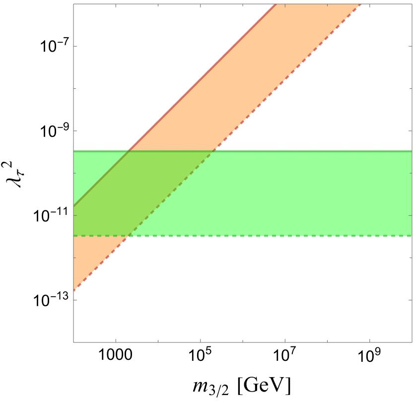
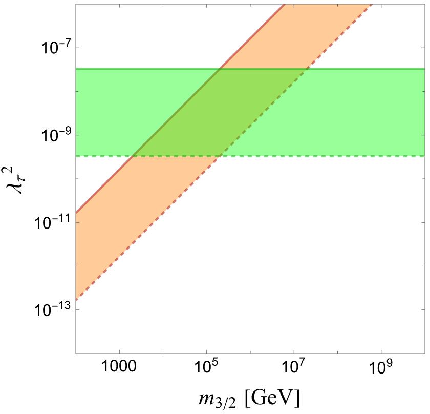
The above observations can also be summarized by comparing the overall scales of the seesaw and -parity contributions to the light neutrino masses. The first is proportional to the parameter given in Eq. (III.1) which goes as . The second is determined as and it is independent of for the fixed gaugino mass scale as can be observed from the expression of in Eq. (62). The requirement that and are of a similar order, therefore, puts an upper bound on as it is shown in Fig. 1. Further, if one chooses , both the contributions scale as leading to a situation similar to the one obtained in the case of conformal discussed in section II.
IV Majoron-neutrino couplings
In the present framework, there exists a Goldstone boson of the spontaneously broken LN symmetry, namely the Majoron Chikashige et al. (1981). It can be identified as
| (65) |
where is the scale of the breaking and the subscript denotes the imaginary part of the corresponding scalar field. The Majoron is an singlet and does not directly couple to the SM neutrinos. However, this coupling is generated through (a) light-heavy neutrino mixing and (b) neutrino-neutralino mixing. This coupling can be parametrized as
| (66) |
in the physical neutrino basis.
The strongest limits on arise from the precision measurement of the acoustic peak of the CMB spectrum which requires that neutrinos must be free streaming at the time of photon decoupling and therefore cannot couple strongly to a nearly massless Majoron. This requirement translates into Hannestad and Raffelt (2005); Raffelt and Weiss (1995); Ayala et al. (2014)
| (67) |
for and . We now show that these limits are satisfied in the model in spite of relatively low LN breaking scale without conflicting with constraints from neutrino masses and mixing.
Contribution to arising from the light-heavy neutrino mixing in the present model can be estimated as follows. Eq. (25) gives rise to the following interaction between the heavy neutrinos and the Majoron:
| (68) |
Subsequently, the couplings with light neutrinos can be estimated using the diagonalization of the relevant blocks of . The latter can be block diagonalized at the leading order by a unitary matrix,
| (69) |
such that is a block diagonal matrix. Here,
| (70) |
The neutral fermions in the block-diagonal basis are given by . Writing the light neutrinos in block diagonal basis as and using Eq. (70), one finds
| (71) |
Substituting the above in Eq. (68) and using the definition of in Eq. (65), we find the light neutrino-Majoron interaction as
| (72) |
with
| (73) | |||||
where we use Eq. (12) to arrive at the last equality. In the above, we have used where are the mass eigenstates which are identified as physical light neutrinos. The couplings are suppressed by as a consequence of heavy-light mixing.
The second contribution arises from the Yukawa interaction in Eq. (25) and through gauge interactions quantified by the following terms:
| (74) |
where and . The Higgsino, Bino and Wino contain the light neutrinos through mixing. From the block diagonalization, one finds
| (75) |
Substituting the above in Eq. (74) and using Eq. (65), we find
| (76) |
where
| (77) |
where is as defined in Eq. (18).
Combining the two contributions and using the definition Eq. (66), the light neutrino-Majoron coupling matrix can be written as
| (78) |
Note that the quantity in the bracket above is the effective neutrino mass matrix in the limit . Therefore, using the simplified expression of obtained in Eq. (58) with , we can express
| (79) |
with
| (80) |
and as defined in Eq. (22). When , the matrix in the bracket in Eq. (79) is identified with and becomes a diagonal matrix leading to only nonzero. This case is relatively poorly constrained as seen from the limits in Eq. (IV).
Numerically, all the dimensionless parameters appearing in the matrix shown in Eq. (79) are of order one as can be seen from the numbers in Tables 1 and 2. The overall scale of neutrino-majoron coupling, therefore, is given by . Also noting that the numerator in Eq. (80) is in the limit , one can estimate an overall size of as
| (81) |
It is seen that remains suppressed for a large range in the parameter space. The matrix appearing in Eq. (78) is also completely determined by the fits of the table since . For example, for solution NH8 listed in Table 1, we get
| (82) |
We find that all the solutions listed in Tables 1 and 2 satisfy the constraints, Eq. (IV), for GeV.
V Majoron-Charged lepton couplings
As in the case of the neutrinos, the charged leptons do not directly couple to Majoron but these couplings arise from their mixing with the charginos. In general, the Majoron-charged lepton couplings can be parametrized as
| (83) |
Majoron has both the diagonal and the off-diagonal couplings. The latter is constrained from the flavour violating decays such as Albrecht et al. (1995); Jodidio et al. (1986). Non-observation of these implies Raffelt and Weiss (1995); Ayala et al. (2014):
| (84) |
The requirement that the red giant stars do not lose energy through Majoron emission from electrons constrain , namely
| (85) |
Despite such strong constraints, a Majoron with breaking scale as low as GeV can satisfy the above limits as we discuss in detail below.
The three charged lepton and two chargino fields can be represented as
| (86) |
with
| (87) |
The charged fermion mass term is parametrized by
| (88) |
where matrix is defined as
| (89) |
Here, denotes the (diagonal) charged lepton mass matrix before mixing with charginos. , arise from the -parity violation and are given by
| (90) |
is the usual chargino mass matrix in the MSSM,
| (91) |
Next, we define a basis
| (92) |
such that assumes a block diagonal form in this basis. Explicitly,
| (93) |
The can be parameterized as
| (94) |
It is always possible Grimus and Lavoura (2000) to choose matrices which puts in the block diagonal form of Eq. (93).
The coupling between the Majoron and charged lepton can be directly obtained from the basic Lagrangian as done in the case of neutrinos. Alternatively, one can use the effective Lagrangian describing the coupling of Majoron to the divergence of the broken current ,
| (95) |
Here,
| (96) |
is the leptonic current in the flavour basis. denotes the symmetry breaking scale as already defined in the previous section. The mixing terms and violate and hence contribute to . This contribution is given by
| (97) |
where
| (98) |
are the diagonal charge matrices representing charges of the underlying charged leptons and charginos. Eq. (97) can be rewritten in the block diagonal basis as
| (99) |
Using Eqs. (93,94), the Majoron charged lepton coupling can be written in the block diagonal basis as
| (100) |
Comparing with the definition Eq. (83), we get
| (101) |
This equation is valid to all orders in the seesaw expansion. is the effective charged lepton mass matrix whose eigenvalues correspond to the masses of the charged leptons.
can be iteratively determined using Eq. (93) in the seesaw approximation . At the leading order, one finds Grimus and Lavoura (2000)
| (102) |
Substitution of the above in Eq. (101) indicates that the charged lepton-Majoron couplings, at the leading order, are suppressed by two powers of seesaw expansion parameter or . This is different from neutrino-Majoron coupling which goes as at the leading order. The model, therefore, predicts additionally suppressed coupling between the Majoron and the charged leptons.
Explicit computation of using the leading order expressions of and neglecting the terms of , we get
| (103) |
Using Eq. (II.1) and noting that of Eqs. (20,27) are smaller than one, the dominant contribution to comes from the term proportional to . This gives, for example,
| (104) | |||||
where we take which is the largest value among all the solutions listed in Tables 1 and 2. The obtained value of is far below the constraint (85). Similarly, the off-diagonal elements are also found much below the existing constraint, Eq. (84).
VI Right-handed neutrinos and direct search prospects
The three RH neutrinos in the model have masses close to the electroweak scale and they can be produced at colliders if their mixing with the other particles is favourable. In this section, we discuss such possibilities in detail and point out ranges of parameters of the model where the direct detection of RH neutrinos is possible. There are two standard methods of detecting the RH neutrinos, see Deppisch et al. (2015) for a review. The RH neutrinos can couple to the standard and through their mixing with the active neutrinos. The same mixing also causes the decay of the into charged leptons. This leads to dilepton + 2 jet signals which are free from the SM background. Such signals however depend on the fourth power of the RH mixing and are therefore sensitive to relatively large mixing only. It is also possible to probe slightly smaller through a technique involving displaced vertices at the LHC, see for example Helo et al. (2014); Izaguirre and Shuve (2015); Gago et al. (2015); Antusch et al. (2017); Cottin et al. (2018); Abada et al. (2019); Drewes and Hajer (2020); Liu et al. (2019); Drewes et al. (2020); Das et al. (2019).
In the -parity violating supersymmetric models, the RH neutrinos can also mix with the neutralinos and this mixing could be much larger than . In such a situation, the RH neutrinos are produced in the decays of neutralinos and further decay through their mixing with the active neutrinos. Relatively small mixing with active neutrinos can result in the delayed decays of the RH neutrinos which lead to the distinctive displaced vertex signatures as discussed in Lavignac and Medina (2021). We focus on this possibility and discuss it at length in this section.
The RH neutrino mass eigenstates are related to the flavour states as
| (105) |
where diagonalizes the mas matrix given in Eq. (7). Explicitly, is given by
| (106) |
Mixing of with the charged leptons follows from Eqs. (69,105). Specifically, one can write
| (107) |
Using the above relation, we find
| (108) |
The predicted RH mixing, is in agreement with a typical seesaw scenario. For and GeV, one gets . This is much smaller than the current limit from the direct searches, Aad et al. (2019); Sirunyan et al. (2018), see for example, the left panel in Fig. 3. One can raise for a smaller and a larger . For example, and GeV in Eq. (63) gives and leads to . While this is much larger than the typical TeV scale seesaw prediction, this still falls short of the existing limits from the collider searches. Nevertheless, it is possible to probe such or even smaller mixing through the specific displaced vertex signature as suggested in Lavignac and Medina (2021) provided that RH neutrinos are produced through neutralinos.
The mixing between heavy neutrinos and neutralinos, relevant for displaced vertex signatures at the colliders, can be estimated using
| (109) |
Using Eqs. (70,31) and ignoring the term in , we find that only the state has mixing with Higgsinos and gauginos at the leading order. It is given by
| (110) |
Overall, the couplings with Higgsinos are suppressed by only while the ones with Bino (Wino) are suppressed by additional power of (). Replacing by physical states through Eq. (106), we find the heavy neutrino-Higgsino mixing as
| (111) |
As it can be seen, does not mix with Higgssinos at the leading order.
The states and can be efficiently produced in the decays of Higgsinos provided that are smaller than the Higgsino masses. Motivated by this, we look for the values of parameters for which is the lightest among all three RH neutrinos222The role of and can be interchanged by changing the sign of , see Eq. (II.1).. As can be seen from Eq. (II.1), the ratios and depend only on and . By varying the values of these parameters in reasonable ranges, we look for the region in which is the lightest RH neutrino. The results are displayed in Fig. 2 in which the regions shaded in orange correspond to .
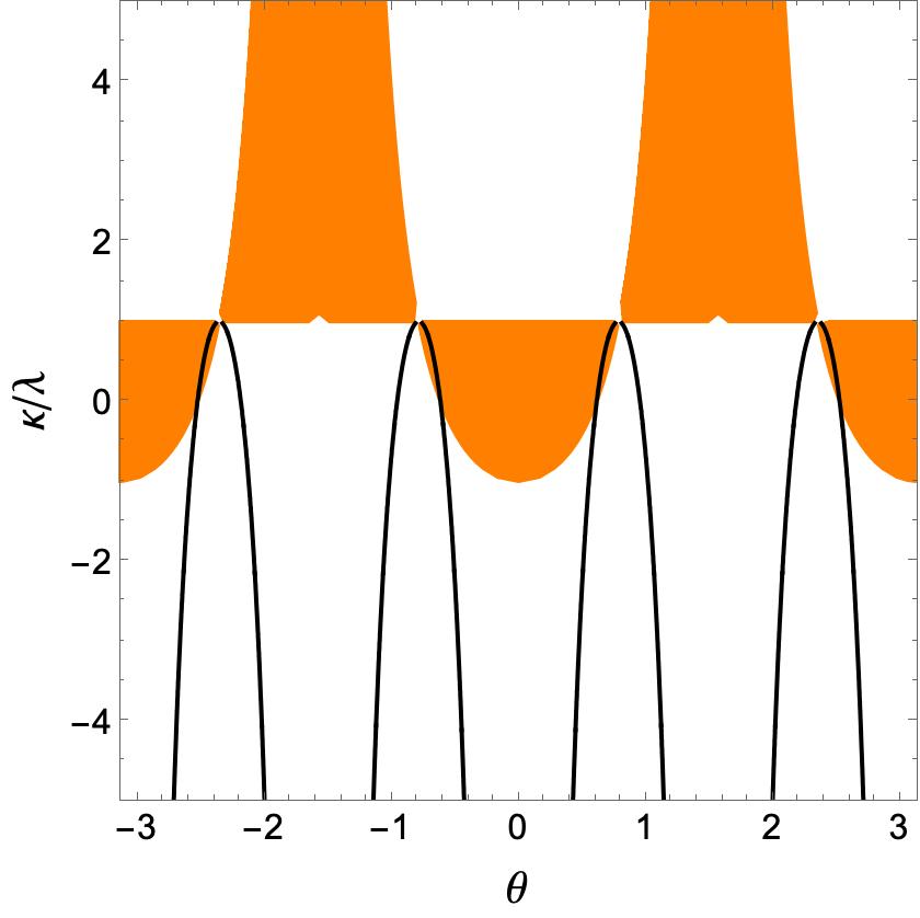
In the same figure, we also show the contours corresponding to
| (112) |
The above arises from a relation between and obtained as Eq. (136) as a result of a specific choice of the soft parameters.
Next, for , we estimate the values of mixing parameters and given in Eq (VI) and (111), respectively. This requires the specification of several parameters. Using Eqs. (26,II.1), we set
| (113) |
For , we use the expression obtained in Eq. (63) and replace using Eq. (9). Also, can be determined from Eq. (61) and using the leading order expression of and also using Eqs. (II.1,10). It leads to
| (114) |
For the MSSM parameters, we take TeV, TeV, GeV, and choose as a specific example. The pair of the lightest neutralinos are dominantly Higgssinos with mass around 500 GeV in this case. With these, and are obtained as functions of , , , and . The first two can be extracted directly from the neutrino mass fits while the next two can be appropriately chosen from Fig. 2 such that is the lightest RH neutrino. We chose and from solution NH8 and randomly vary () in range - (-) and compute and as function of .
The results are displayed in Fig. 3. We also show the typical value of expected naively from a seesaw relation, , as a solid line in the left panel of Fig. 3. The predicted values of can be larger than the typical expectation from seesaw estimates by several orders of magnitude. Also, a number of points for GeV fall either in the already excluded region or are quite close to it.
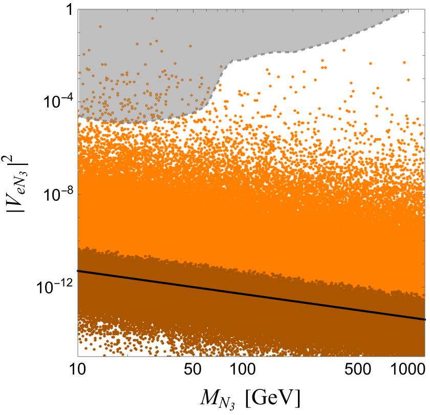
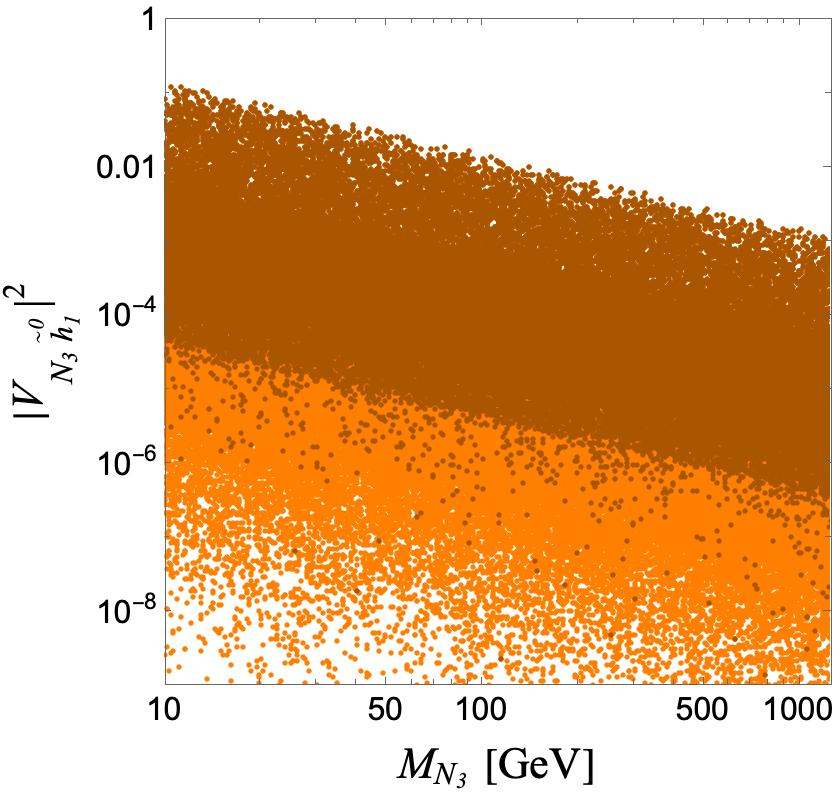
For the Higgssinos with mass around GeV that we have considered in the present analysis, their production cross section at a center-of-mass energy of TeV at the LHC is typically of Fiaschi et al. (2023). This is notably smaller, by six to seven orders of magnitude, than the cross section for -boson production. Nevertheless, the production of RH neutrinos resulting from the latter process is directly proportional to . Consequently, RH neutrinos can be predominantly generated through Higgsinos when the ratio exceeds . In Figure 3, we depict points satisfying in a darker shade. These points stand out as particularly conducive to the production of RH neutrinos through Higgsinos. A dedicated analysis of the expected number of events would be needed to firmly establish the observability or otherwise of the RH neutrinos through the search of the displaced vertices at the LHC. We note however that a similar analysis for two specific benchmark points is already done in Lavignac and Medina (2021) where and are shown to lead to observable displaced vertices at the LHC for GeV and for the similar values of and . The magnitudes of and obtained for GeV in Fig. 3 are comparable and may even lean towards being somewhat larger. Hence, the parameter range within the current model presents an opportunity to investigate RH neutrinos in the direct search experiments, particularly when their signatures through conventional processes are suppressed.
VII Discussions
Extension of the SM to include the LN as an explicit global or local symmetry is primarily aimed at providing tiny but non-vanishing masses for the light neutrinos through the seesaw mechanisms. On the other hand, extension with enlarged space-time symmetries such as supersymmetry is aimed to ameliorate some structural issues pertaining to the SM. In general, these are two separate classes of new physics and they may be operating at two different scales. They are often combined to play complementary roles. A more intriguing possibility is that both these frameworks arise from a common mechanism and, therefore, their scales are closely related. We have put forward one such mechanism and discussed its most relevant phenomenological aspects in detail.
The mechanism uses a global LN symmetry and three SM singlet superfields, two of which are charged under the . The Lorentz scalar components of these superfields acquire non-zero vacuum expectation values and break spontaneously only when the soft terms in supergravity are switched on. This relates the breaking scale with the SUSY breaking scale which is proportional to the gravitino mass . The fermionic components of the SM singlet superfields which play the role of RH neutrinos also get masses of order . The same scale also governs the neutrino-neutralino mixing through -parity violation effectively induced by the VEVs of the SM singlet scalars. It is also possible to link the MSSM -parameter with the common scale utilising the vacuum structure of the RH sneutrinos.
The identification of various scales with a common scale in the underlying framework leads to the following interesting and noteworthy observations:
-
•
The light neutrinos acquire masses through the usual seesaw mechanism as well as from -parity violation. The realistic neutrino mass spectrum requires that both these contributions are of similar magnitude. In the case of (i.e. conformal superpotential), both these contributions are proportional to . Therefore, the usual scale of the seesaw would also imply high-scale SUSY. On the other hand, keeping the SUSY scale close to the electroweak scale necessarily leads to low scale seesaw mechanism with RH neutrino masses of the order of a few hundred GeV.
-
•
If is kept independent of and held fixed close to the electroweak scale, the viable light neutrino masses do not allow a large hierarchy between and . This again implies a low-scale seesaw mechanism and a SUSY breaking scale not very far from the electroweak scale. In particular, the gauginos and RH neutrinos are not allowed to be arbitrarily heavy in this case.
-
•
The spontaneous breaking of at the scale leads to a Majoron with coupling to the light neutrinos of . This turns out to be small enough to satisfy all the present constraints even for massless Majoron.
-
•
The framework offers an interesting possibility of probing the existence of near weak-scale RH neutrinos through their displaced vertex signature in which they are produced dominantly from Higgssinos at the colliders and subsequently decay into the SM particles. It is seen that for a range of parameters, the model predicts sizeable mixings between Higgssino and RH neutrino and between the heavy and light neutrinos enhancing the possibility for direct detection.
All along, we have assumed that supergravity is responsible for the generation of the soft SUSY breaking. However, the underlying mechanism is applicable even if the SUSY breaking arises from some other sources.
The basic framework presented in this work utilizes an exact global LN symmetry which is spontaneously broken through soft SUSY breaking terms. The considered superpotential and the soft terms in the conformal case also possess a discrete symmetry. It is known that the spontaneous breaking of these exact symmetries lead to formation of topological defects like comic strings and domain walls. However, small explicit breaking of such symmetries, possibly induced through gravity effects (see for example, Rothstein et al. (1993); Akhmedov et al. (1992, 1993)), can make these structures unstable. For example, spontaneous breaking of an approximate global is shown to lead to strings connected by domain walls which decay quickly and do not dominate the universe Vilenkin and Everett (1982). Similarly, the domain walls produced due to breaking can be made to disappear effectively before nucleosynthesis if Planck scale suppressed explicit breaking terms are introduced Panagiotakopoulos and Tamvakis (1999). From a phenomenological standpoint, explicitly breaking LN results in a small mass for the Majoron the exact magnitude of which depends on the nature of the breaking. While it could also contribute to light and heavy neutrino masses, the impact remains negligibly small with Planck scale suppressed LN symmetry breaking. Thus, small explicit breaking of the underlying global symmetries can address cosmological concerns without significantly altering the primary mechanism for neutrino mass generation presented in this study. The non-conformal case considered here does not have a discrete symmetry and is thus free from the domain wall problem.
Acknowledgements
This work is partially supported under the MATRICS project (MTR/2021/000049) by the Science & Engineering Research Board (SERB), Department of Science and Technology (DST), Government of India. KMP acknowledges support from the ICTP through the Associates Programme (2023-2028) where part of this work was completed.
Appendix A Potential minimization and VEVs of RH sneutrinos
In this Appendix, we provide a derivation of the vacuum expectation values given in Eq. (4). The relevant scalar potential of the model derived from in Eq. (1) along with the soft terms is obtained as
| (115) |
where is given in Eq. (3).
We parametrize the VEVs of the three scalar fields as
| (116) |
The parameters , and are to be obtained by solving the minimization conditions at the minimum for . For simplicity, we assume all the parameters in real and also require real solutions for the VEVs. Using a linear combination of two of the minimization conditions
| (117) |
we obtain
| (118) |
at the minimum of the potential. Using the orthogonal linear combination
| (119) |
we solve for and obtain
| (120) |
Next, we assume for simplification which leads to and degenerate VEVs for and . Using the remaining minimization condition, , and substituting the non-vanishing solution for given in Eq. (120) along with , we find the following equation:
| (121) |
with
| (122) |
The other solution, , leads to . Eq. (121) needs to be solved to determine which then can be used to find the VEVs in terms of the parameters of the scalar potential.
It is convenient to convert Eq. (121) into the so-called “Depressed cubic” equation Dickson by the following change of variable:
| (123) |
In the new variable, the equation has no quadratic term and it is given by
| (124) |
where
| (125) |
The discriminant of the Depressed cubic equation is given by
| (126) |
The following possibilities exist for the solutions Dickson of Eq. (124):
-
•
If , then the underlying polynomial has three distinct real roots. They are explicitly given by
(127) -
•
For and , the polynomial has three real roots out of which two are degenerate. These are
(128) -
•
If then the polynomial has one real and two complex roots. The real root can be represented, for , as
(129) and, for , as
(130)
Substituting , and from Eq. (A) in Eq. (A), one can determine which turns out to be proportional to . With an appropriate choice of the values of the soft parameters, can be obtained leading to the real solutions for .
As an explicit example, consider
| (131) |
This leads to for which the roots can be estimated from Eq. (128). Substituting this choice of the soft parameters in Eq. (A) and using Eq. (128) and (123), we find the real solutions as
| (132) |
Substitution of the above in expression Eq. (120) leads to
| (133) |
The first solution leads to an imaginary while the second corresponds to real if . Moreover, the solution corresponding to is a global minimum.
In summary, for , the scalar potential given in Eq. (115) can lead to the following VEV configuration:
| (134) |
where and are dimensionless parameters determined by , and the soft parameters. The non-trivial relation between the VEVs obtained in Eq. (120) implies the following correlation between and :
| (135) |
For the specific choice of the soft terms used in Eq. (131) and the resulting in Eq. (132), the above becomes
| (136) |
which is completely determined in terms of the ratio . However, the desired value of and can be obtained by the appropriate choice of and in general. Therefore, the VEVs in Eq. (134) are parametrized in a general way and considered for phenomenological analysis.
Appendix B Calculation of
We derive expressions for displayed in Eqs. (20,27) in this Appendix following a similar calculation carried out earlier in Giudice et al. (1993); Joshipura et al. (2002) for a different framework. When the scalar components of take VEVs, the bilinear terms in are given by
| (137) |
Here, and we consider a general case in which contains both the contributions such as shown in Eq. (26). The scalar potential evaluated from the above is then given by
| (138) | |||||
where the last term in the first line arises from the -term of . Further, the relevant soft terms can be written as
| (139) | |||||
where we have defined
| (140) |
Rotating away the term proportional to form Eq. (137) using the redefinitions:
| (141) |
one finds that and get modified to
| (142) | |||||
In the new basis, the VEV of the electrically neutral components of the are denoted by . It is related to the VEV in the original basis by Eq. (141). Using the defining relation, , and minimizing the potential , we obtain
| (143) |
Neglecting the contributions of , the above can be further simplified to
| (144) |
The first term in is suppressed for the universal soft masses. Depending on the presence or absence of bare in the model, the nature of the second term in can be decided. For example, when , using Eq. (140) and the fact that , Eq. (144) can be reduced to
| (145) |
Both terms in can then be suppressed for the universal soft terms.
References
- Weinberg (1979) Steven Weinberg, “Baryon and Lepton Nonconserving Processes,” Phys. Rev. Lett. 43, 1566–1570 (1979).
- Mohapatra et al. (2007) R. N. Mohapatra et al., “Theory of neutrinos: A White paper,” Rept. Prog. Phys. 70, 1757–1867 (2007), arXiv:hep-ph/0510213 .
- Minkowski (1977) Peter Minkowski, “ at a Rate of One Out of Muon Decays?” Phys. Lett. B 67, 421–428 (1977).
- Yanagida (1979) Tsutomu Yanagida, “Horizontal gauge symmetry and masses of neutrinos,” Conf. Proc. C 7902131, 95–99 (1979).
- Mohapatra and Senjanovic (1980) Rabindra N. Mohapatra and Goran Senjanovic, “Neutrino Mass and Spontaneous Parity Nonconservation,” Phys. Rev. Lett. 44, 912 (1980).
- Schechter and Valle (1980) J. Schechter and J. W. F. Valle, “Neutrino masses in su(2) u(1) theories,” Phys. Rev. D 22, 2227–2235 (1980).
- Fritzsch and Minkowski (1975) Harald Fritzsch and Peter Minkowski, “Unified Interactions of Leptons and Hadrons,” Annals Phys. 93, 193–266 (1975).
- Gell-Mann et al. (1979) Murray Gell-Mann, Pierre Ramond, and Richard Slansky, “Complex Spinors and Unified Theories,” Conf. Proc. C 790927, 315–321 (1979), arXiv:1306.4669 [hep-th] .
- Martin (1998) Stephen P. Martin, “A Supersymmetry primer,” Adv. Ser. Direct. High Energy Phys. 18, 1–98 (1998), arXiv:hep-ph/9709356 .
- Dimopoulos and Georgi (1981) Savas Dimopoulos and Howard Georgi, “Softly Broken Supersymmetry and SU(5),” Nucl. Phys. B 193, 150–162 (1981).
- Dimopoulos et al. (1981) S. Dimopoulos, S. Raby, and Frank Wilczek, “Supersymmetry and the Scale of Unification,” Phys. Rev. D 24, 1681–1683 (1981).
- Marciano and Senjanovic (1982) William J. Marciano and Goran Senjanovic, “Predictions of Supersymmetric Grand Unified Theories,” Phys. Rev. D 25, 3092 (1982).
- Arkani-Hamed and Dimopoulos (2005) Nima Arkani-Hamed and Savas Dimopoulos, “Supersymmetric unification without low energy supersymmetry and signatures for fine-tuning at the LHC,” JHEP 06, 073 (2005), arXiv:hep-th/0405159 .
- Giudice and Romanino (2004) G. F. Giudice and A. Romanino, “Split supersymmetry,” Nucl. Phys. B 699, 65–89 (2004), [Erratum: Nucl.Phys.B 706, 487–487 (2005)], arXiv:hep-ph/0406088 .
- Lahanas and Nanopoulos (1987) A. B. Lahanas and Dimitri V. Nanopoulos, “The Road to No Scale Supergravity,” Phys. Rept. 145, 1 (1987).
- Lopez-Fogliani and Munoz (2006) D. E. Lopez-Fogliani and C. Munoz, “Proposal for a Supersymmetric Standard Model,” Phys. Rev. Lett. 97, 041801 (2006), arXiv:hep-ph/0508297 .
- Escudero et al. (2008) Nicolas Escudero, Daniel E. Lopez-Fogliani, Carlos Munoz, and Roberto Ruiz de Austri, “Analysis of the parameter space and spectrum of the mu nu SSM,” JHEP 12, 099 (2008), arXiv:0810.1507 [hep-ph] .
- Ghosh and Roy (2009) Pradipta Ghosh and Sourov Roy, “Neutrino masses and mixing, lightest neutralino decays and a solution to the mu problem in supersymmetry,” JHEP 04, 069 (2009), arXiv:0812.0084 [hep-ph] .
- Fidalgo et al. (2009) Javier Fidalgo, Daniel E. Lopez-Fogliani, Carlos Munoz, and R. Ruiz de Austri, “Neutrino Physics and Spontaneous CP Violation in the mu nu SSM,” JHEP 08, 105 (2009), arXiv:0904.3112 [hep-ph] .
- Lopez-Fogliani and Munoz (2020) Daniel E. Lopez-Fogliani and Carlos Munoz, “Searching for supersymmetry: the SSM: A short review,” Eur. Phys. J. ST 229, 3263–3301 (2020), arXiv:2009.01380 [hep-ph] .
- Ibanez and Ross (1982) Luis E. Ibanez and Graham G. Ross, “SU(2)-L x U(1) Symmetry Breaking as a Radiative Effect of Supersymmetry Breaking in Guts,” Phys. Lett. B 110, 215–220 (1982).
- Chun et al. (1995) E. J. Chun, Anjan S. Joshipura, and A. Yu. Smirnov, “Models of light singlet fermion and neutrino phenomenology,” Phys. Lett. B 357, 608–615 (1995), arXiv:hep-ph/9505275 .
- Chun et al. (1996) Eung Jin Chun, Anjan S. Joshipura, and Alexei Yu. Smirnov, “QuasiGoldstone fermion as a sterile neutrino,” Phys. Rev. D 54, 4654–4661 (1996), arXiv:hep-ph/9507371 .
- Chun (1999) Eung Jin Chun, “Axino neutrino mixing in gauge mediated supersymmetry breaking models,” Phys. Lett. B 454, 304–308 (1999), arXiv:hep-ph/9901220 .
- Choi et al. (2001) Kiwoon Choi, Eung Jin Chun, and Kyuwan Hwang, “Axino as a sterile neutrino and R-parity violation,” Phys. Rev. D 64, 033006 (2001), arXiv:hep-ph/0101026 .
- Lavignac and Medina (2021) Stéphane Lavignac and Anibal D. Medina, “Displaced Vertex signatures of a pseudo-Goldstone sterile neutrino,” JHEP 01, 151 (2021), arXiv:2010.00608 [hep-ph] .
- Joshipura and Patel (2021) Anjan S. Joshipura and Ketan M. Patel, “Weak scale right-handed neutrino as pseudo-Goldstone fermion of spontaneously broken ,” JHEP 09, 115 (2021), arXiv:2107.12802 [hep-ph] .
- Ellwanger et al. (2010) Ulrich Ellwanger, Cyril Hugonie, and Ana M. Teixeira, “The Next-to-Minimal Supersymmetric Standard Model,” Phys. Rept. 496, 1–77 (2010), arXiv:0910.1785 [hep-ph] .
- Masiero and Valle (1990) A. Masiero and J. W. F. Valle, “A Model for Spontaneous R Parity Breaking,” Phys. Lett. B 251, 273–278 (1990).
- Barbier et al. (2005) R. Barbier et al., “R-parity violating supersymmetry,” Phys. Rept. 420, 1–202 (2005), arXiv:hep-ph/0406039 .
- Mohapatra and Valle (1986) R. N. Mohapatra and J. W. F. Valle, “Neutrino Mass and Baryon Number Nonconservation in Superstring Models,” Phys. Rev. D 34, 1642 (1986).
- Mohapatra (1986) R. N. Mohapatra, “Mechanism for Understanding Small Neutrino Mass in Superstring Theories,” Phys. Rev. Lett. 56, 561–563 (1986).
- Nandi and Sarkar (1986) S. Nandi and U. Sarkar, “A Solution to the Neutrino Mass Problem in Superstring E6 Theory,” Phys. Rev. Lett. 56, 564 (1986).
- Joshipura et al. (2002) Anjan S. Joshipura, Rishikesh D. Vaidya, and Sudhir K. Vempati, “Bi maximal mixing and bilinear R violation,” Nucl. Phys. B 639, 290–306 (2002), arXiv:hep-ph/0203182 .
- Grimus and Löschner (2018) W. Grimus and M. Löschner, “Renormalization of the multi-Higgs-doublet Standard Model and one-loop lepton mass corrections,” JHEP 11, 087 (2018), arXiv:1807.00725 [hep-ph] .
- Romao et al. (2000) J. C. Romao, M. A. Diaz, M. Hirsch, W. Porod, and J. W. F Valle, “A Supersymmetric solution to the solar and atmospheric neutrino problems,” Phys. Rev. D 61, 071703 (2000), arXiv:hep-ph/9907499 .
- Hirsch et al. (2000) M. Hirsch, M. A. Diaz, W. Porod, J. C. Romao, and J. W. F. Valle, “Neutrino masses and mixings from supersymmetry with bilinear R parity violation: A Theory for solar and atmospheric neutrino oscillations,” Phys. Rev. D 62, 113008 (2000), [Erratum: Phys.Rev.D 65, 119901 (2002)], arXiv:hep-ph/0004115 .
- Capozzi et al. (2017) Francesco Capozzi, Eleonora Di Valentino, Eligio Lisi, Antonio Marrone, Alessandro Melchiorri, and Antonio Palazzo, “Global constraints on absolute neutrino masses and their ordering,” Phys. Rev. D 95, 096014 (2017), [Addendum: Phys.Rev.D 101, 116013 (2020)], arXiv:2003.08511 [hep-ph] .
- de Salas et al. (2021) P. F. de Salas, D. V. Forero, S. Gariazzo, P. Martínez-Miravé, O. Mena, C. A. Ternes, M. Tórtola, and J. W. F. Valle, “2020 global reassessment of the neutrino oscillation picture,” JHEP 02, 071 (2021), arXiv:2006.11237 [hep-ph] .
- Esteban et al. (2020) Ivan Esteban, M. C. Gonzalez-Garcia, Michele Maltoni, Thomas Schwetz, and Albert Zhou, “The fate of hints: updated global analysis of three-flavor neutrino oscillations,” JHEP 09, 178 (2020), arXiv:2007.14792 [hep-ph] .
- Giudice and Rattazzi (1999) G. F. Giudice and R. Rattazzi, “Theories with gauge mediated supersymmetry breaking,” Phys. Rept. 322, 419–499 (1999), arXiv:hep-ph/9801271 .
- Chikashige et al. (1981) Y. Chikashige, Rabindra N. Mohapatra, and R. D. Peccei, “Are There Real Goldstone Bosons Associated with Broken Lepton Number?” Phys. Lett. B 98, 265–268 (1981).
- Hannestad and Raffelt (2005) Steen Hannestad and Georg Raffelt, “Constraining invisible neutrino decays with the cosmic microwave background,” Phys. Rev. D 72, 103514 (2005), arXiv:hep-ph/0509278 .
- Raffelt and Weiss (1995) Georg Raffelt and Achim Weiss, “Red giant bound on the axion - electron coupling revisited,” Phys. Rev. D 51, 1495–1498 (1995), arXiv:hep-ph/9410205 .
- Ayala et al. (2014) Adrian Ayala, Inma Domínguez, Maurizio Giannotti, Alessandro Mirizzi, and Oscar Straniero, “Revisiting the bound on axion-photon coupling from Globular Clusters,” Phys. Rev. Lett. 113, 191302 (2014), arXiv:1406.6053 [astro-ph.SR] .
- Albrecht et al. (1995) H. Albrecht et al. (ARGUS), “A Search for lepton flavor violating decays tau e alpha, tau mu alpha,” Z. Phys. C 68, 25–28 (1995).
- Jodidio et al. (1986) A. Jodidio, B. Balke, J. Carr, G. Gidal, K. A. Shinsky, H. M. Steiner, D. P. Stoker, M. Strovink, R. D. Tripp, B. Gobbi, and C. J. Oram, “Search for right-handed currents in muon decay,” Phys. Rev. D 34, 1967–1990 (1986).
- Grimus and Lavoura (2000) W. Grimus and L. Lavoura, “The Seesaw mechanism at arbitrary order: Disentangling the small scale from the large scale,” JHEP 11, 042 (2000), arXiv:hep-ph/0008179 .
- Deppisch et al. (2015) Frank F. Deppisch, P. S. Bhupal Dev, and Apostolos Pilaftsis, “Neutrinos and Collider Physics,” New J. Phys. 17, 075019 (2015), arXiv:1502.06541 [hep-ph] .
- Helo et al. (2014) Juan C. Helo, Martin Hirsch, and Sergey Kovalenko, “Heavy neutrino searches at the LHC with displaced vertices,” Phys. Rev. D 89, 073005 (2014), [Erratum: Phys.Rev.D 93, 099902 (2016)], arXiv:1312.2900 [hep-ph] .
- Izaguirre and Shuve (2015) Eder Izaguirre and Brian Shuve, “Multilepton and Lepton Jet Probes of Sub-Weak-Scale Right-Handed Neutrinos,” Phys. Rev. D 91, 093010 (2015), arXiv:1504.02470 [hep-ph] .
- Gago et al. (2015) Alberto M. Gago, Pilar Hernández, Joel Jones-Pérez, Marta Losada, and Alexander Moreno Briceño, “Probing the Type I Seesaw Mechanism with Displaced Vertices at the LHC,” Eur. Phys. J. C 75, 470 (2015), arXiv:1505.05880 [hep-ph] .
- Antusch et al. (2017) Stefan Antusch, Eros Cazzato, and Oliver Fischer, “Sterile neutrino searches via displaced vertices at LHCb,” Phys. Lett. B 774, 114–118 (2017), arXiv:1706.05990 [hep-ph] .
- Cottin et al. (2018) Giovanna Cottin, Juan Carlos Helo, and Martin Hirsch, “Displaced vertices as probes of sterile neutrino mixing at the LHC,” Phys. Rev. D 98, 035012 (2018), arXiv:1806.05191 [hep-ph] .
- Abada et al. (2019) Asmaa Abada, Nicolás Bernal, Marta Losada, and Xabier Marcano, “Inclusive Displaced Vertex Searches for Heavy Neutral Leptons at the LHC,” JHEP 01, 093 (2019), arXiv:1807.10024 [hep-ph] .
- Drewes and Hajer (2020) Marco Drewes and Jan Hajer, “Heavy Neutrinos in displaced vertex searches at the LHC and HL-LHC,” JHEP 02, 070 (2020), arXiv:1903.06100 [hep-ph] .
- Liu et al. (2019) Jia Liu, Zhen Liu, Lian-Tao Wang, and Xiao-Ping Wang, “Seeking for sterile neutrinos with displaced leptons at the LHC,” JHEP 07, 159 (2019), arXiv:1904.01020 [hep-ph] .
- Drewes et al. (2020) Marco Drewes, Andrea Giammanco, Jan Hajer, and Michele Lucente, “New long-lived particle searches in heavy-ion collisions at the LHC,” Phys. Rev. D 101, 055002 (2020), arXiv:1905.09828 [hep-ph] .
- Das et al. (2019) Arindam Das, P. S. Bhupal Dev, and Nobuchika Okada, “Long-lived TeV-scale right-handed neutrino production at the LHC in gauged model,” Phys. Lett. B 799, 135052 (2019), arXiv:1906.04132 [hep-ph] .
- Aad et al. (2019) Georges Aad et al. (ATLAS), “Search for heavy neutral leptons in decays of bosons produced in 13 TeV collisions using prompt and displaced signatures with the ATLAS detector,” JHEP 10, 265 (2019), arXiv:1905.09787 [hep-ex] .
- Sirunyan et al. (2018) Albert M Sirunyan et al. (CMS), “Search for heavy neutral leptons in events with three charged leptons in proton-proton collisions at 13 TeV,” Phys. Rev. Lett. 120, 221801 (2018), arXiv:1802.02965 [hep-ex] .
- Fiaschi et al. (2023) Juri Fiaschi, Benjamin Fuks, Michael Klasen, and Alexander Neuwirth, “Electroweak superpartner production at 13.6 Tev with Resummino,” Eur. Phys. J. C 83, 707 (2023), arXiv:2304.11915 [hep-ph] .
- Rothstein et al. (1993) I. Z. Rothstein, K. S. Babu, and D. Seckel, “Planck scale symmetry breaking and majoron physics,” Nucl. Phys. B 403, 725–748 (1993), arXiv:hep-ph/9301213 .
- Akhmedov et al. (1992) Evgeny K. Akhmedov, Zurab G. Berezhiani, and Goran Senjanovic, “Planck scale physics and neutrino masses,” Phys. Rev. Lett. 69, 3013–3016 (1992), arXiv:hep-ph/9205230 .
- Akhmedov et al. (1993) Evgeny K. Akhmedov, Z. G. Berezhiani, R. N. Mohapatra, and G. Senjanovic, “Planck scale effects on the majoron,” Phys. Lett. B 299, 90–93 (1993), arXiv:hep-ph/9209285 .
- Vilenkin and Everett (1982) A. Vilenkin and A. E. Everett, “Cosmic Strings and Domain Walls in Models with Goldstone and PseudoGoldstone Bosons,” Phys. Rev. Lett. 48, 1867–1870 (1982).
- Panagiotakopoulos and Tamvakis (1999) C. Panagiotakopoulos and K. Tamvakis, “Stabilized NMSSM without domain walls,” Phys. Lett. B 446, 224–227 (1999), arXiv:hep-ph/9809475 .
- (68) Leonard Eugene Dickson, “First course in the theory of equations,” Nature 109, 773–774.
- Giudice et al. (1993) G. F. Giudice, A. Masiero, M. Pietroni, and A. Riotto, “The Supersymmetric singlet majoron,” Nucl. Phys. B 396, 243–260 (1993), arXiv:hep-ph/9209296 .