The statistical thermodynamics of generative diffusion models

Abstract

Generative diffusion models have achieved spectacular performance in many areas of generative modeling. While the fundamental ideas behind these models come from non-equilibrium physics, in this paper we show that many aspects of these models can be understood using the tools of equilibrium statistical mechanics. Using this reformulation, we show that generative diffusion models undergo second-order phase transitions corresponding to symmetry breaking phenomena. We argue that this lead to a form of instability that lies at the heart of their generative capabilities and that can be described by a set of mean field critical exponents. We conclude by analyzing recent work connecting diffusion models and associative memory networks in view of the thermodynamic formulations.

1 Introduction

Generative modeling is a sub-field of machine learning concerned with the automatic generation of structured data such as images, videos and written language (Bond-Taylor et al.,, 2021). Generative diffusion models (Sohl-Dickstein et al.,, 2015), also known as score-based models, form a class of deep generative models that have demonstrated high performance in image (Ho et al.,, 2020; Song et al., 2021b, ), sound (Chen et al.,, 2020; Kong et al.,, 2020; Liu et al.,, 2023) and video generation (Ho et al.,, 2022; Singer et al.,, 2022). Diffusion models were first introduced in analogy with the physics of non-equilibrium statistical physics. The fundamental idea is to formalize generation as the probabilistic inverse of a forward stochastic process that gradually turns the target distribution $\phi(\boldsymbol{y})$ into a simple base distribution such as Gaussian white noise (Sohl-Dickstein et al.,, 2015; Song et al., 2021a, ).

In this paper we will show that many of the features of these models can be understood using the tools of equilibrium statistical physics. Specifically, we define a family of Boltzmann distributions over the noise-free states, which can be interpreted as (unobservable) microstates during the diffusion process. Using this reformulation, we show that generative diffusion models can undergo second-order phase transitions of the mean-field type, corresponding the the generative spontaneous symmetry breaking fist discussed in (Raya and Ambrogioni,, 2023). In this analysis, the diffusion time parameter plays the role of "temperature". We obtain a self-consistent equation of state for the system, which corresponds to the fixed-point equation of the generative dynamics. We also show that the generative dynamics minimizes a regularized Helmholtz free energy, which connects diffusion models to other energy-based models in the machine learning and theoretical neuroscience literature (Friston,, 2010).

2 Preliminaries on generative diffusion models

The goal of diffusion modeling is to sample from a potentially very complex target distribution $\phi(\boldsymbol{y})$. To this end, we shall consider $\phi(\boldsymbol{y})$ as the initial boundary condition of a forward stochastic process that removes structure by injecting white noise. In order to simplify the derivations, we assume the forward process to be a mathematical Brownian motion. Other forward processes are more commonly used in the applied literature, such as the variance preserving process (e.g. a non-stationary Olsten-Uhlenbeck process) (Song et al., 2021b, ). However, most of the qualitative thermodynamic properties are shared between these models. The mathematical Brownian motion is defined by the following Langevin equation:

$$\boldsymbol{x}(t+\text{d}t)=\boldsymbol{x}(t)+~{}\sigma~{}\boldsymbol{w}(t)\sqrt{\text{d}t}$$ (1)

where $\text{d}t$ is an infinitesimal increment, $\sigma$ is the instantaneous standard deviation of the stochastic input and $w(t)$ is a standard Gaussian white noise process. The marginals defined by . 1 with $\phi(\boldsymbol{y})$ as initial boundary condition can be expressed analytically as follows:

$$p_{t}(\boldsymbol{x})=\frac{1}{\sqrt{2\pi t\sigma^{2}}}\mathbb{E}_{\boldsymbol{y}\sim\phi}\!\left[e^{-\frac{{\left\lVert\boldsymbol{x}-\boldsymbol{y}\right\rVert}_{2}^{2}}{2t\sigma^{2}}}\right]$$ (2)

where the expectation is taken with respect to the target distribution $\phi(\boldsymbol{y})$. A generative model can then be obtained by "inverting" Eq. 1. The inverse equation equation is

$$\boldsymbol{x}(t-\text{d}t)=\boldsymbol{x}(t)-\sigma^{2}\nabla\log{p_{t}(\boldsymbol{x})}+~{}\sigma~{}w(t)\sqrt{\text{d}t}~{},$$ (3)

which can be shown to give the same marginal distributions in Eq. 2 if the process is initialized with appropriately scaled white-noise (Anderson,, 1982). The function $\nabla\log{p_{t}(\boldsymbol{x})}$ is known as the score in the literature. If the score is available for all values of $\boldsymbol{x}$ and $t$, we can then sample from $\phi(\boldsymbol{y})$ by integrating Eq. 3 using numerical methods.

2.1 Training diffusion models as denoising autoencoders

Figure 1: Generative process for a digit taken from the MNIST dataset.

While the score of the target distribution is generally not available analytically, a deep network can be trained to approximate it using a from a large set of samples (Song et al., 2021a, ). We refer to the network as a vector valued function $\boldsymbol{f}(\boldsymbol{x}(t),t)$. Deep network are parameterized by a large number of weights and biases. However, since we are not interested in the details of the specific parameterization, here we will report the functional loss:

$$\mathcal{L}\left[f(\cdot,\cdot)\right]=\int_{0}^{t_{\text{end}}}\mathbb{E}_{\boldsymbol{y},\boldsymbol{x}(t)}\!\left[\frac{1}{2}{\left\lVert\boldsymbol{y}-\boldsymbol{f}(\boldsymbol{x}(t),t)\right\rVert}_{2}^{2}\right]\text{d}\Psi(t)~{},$$ (4)

where $\Psi(t)$ is a cumulative distribution with support in $(0,t_{\text{end}})$ and $\boldsymbol{x}(t)$ is sampled conditional on $\boldsymbol{y}$ using the propagator of the forward Langevin equation. The score function $\nabla\log{p_{t}(\boldsymbol{x})}$ can then be obtained from the optimized network $\mathbf{f}^{*}=\text{argmin}~{}\mathcal{L}\left[f\right]$ using the following formula (Anderson,, 1982):

$$\nabla\log{p_{t}(\boldsymbol{x})}=(t\sigma^{2})^{-1}\left(f^{*}(\boldsymbol{x}(t),t)-\boldsymbol{x}(t)\right)~{}.$$ (5)

In other words, the score is proportional to the optimal estimate of the noise given the noise-corrupted state. therefore, once the network is trained to minimize Eq. 4, synthetic samples can be generated by sampling $\boldsymbol{x}(t_{\text{end}})$ from the boundary noise, computing the score using Eq. 5 distribution and integrating backward Eq. 3 using numerical methods. An example of this generative dynamics for a network trained on natural images is shown in Fig. 1.

3 Diffusion models as systems in equilibrium

As defined above by the forward and inverse Langevin equation, generative diffusion models are non-equilibrium systems. In this section, we shall show that they can be reformulated using the language of equilibrium statistical mechanics, which will allow us to analyze their thermodynamics properties. The starting point for any model in statistical mechanics is the definition of the relevant microstates. In physics, the microstate is considered an unobservable quantity. If we can observe a noise-corrupted data $\boldsymbol{x}^{*}(t)$, the obvious unobservable quantity of interest is the noise-free initial state $\boldsymbol{x}^{*}(0)=\boldsymbol{y}^{*}$. The next step is to define a Hamiltonian function on the set of microstates and all values of the time $t$. We startcan do this by considering the conditional probability of the data $\boldsymbol{y}$ given a noisy state $\boldsymbol{x}_{t}$:

$$p(\boldsymbol{y}\mid\boldsymbol{x},t)=\frac{1}{p(\boldsymbol{x},t)}e^{-\frac{{\left\lVert\boldsymbol{x}-\boldsymbol{y}\right\rVert}_{2}^{2}}{2t\sigma^{2}}-\log{\phi(\boldsymbol{y})}}=\frac{1}{Z(\boldsymbol{x},t)}e^{-\mathcal{H}(\boldsymbol{y};\boldsymbol{x},t)}~{},$$ (6)

which we can interpret as a Boltzmann distribution over the microstates $\boldsymbol{y}$ with Hamiltonian

$$\mathcal{H}(\boldsymbol{y};\boldsymbol{x},t)=(t\sigma^{2})^{-1}\left(\frac{1}{2}{\left\lVert\boldsymbol{y}\right\rVert}_{2}^{2}-\boldsymbol{x}\cdot\boldsymbol{y}\right)-\log{\phi(\boldsymbol{y})}$$ (7)

and partition function

$$Z(\boldsymbol{x},t)=\int e^{-\mathcal{H}(\boldsymbol{y};\boldsymbol{x},t)}\text{d}\boldsymbol{y}~{}.$$ (8)

The thermodynamic system defined by Eq. 6 does not have a true temperature parameter. However, the quantity $\sigma t$ plays a very similar role to temperature in classical statistical mechanics. Moreover, in the Hamiltonian given by Eq .7, the dynamic variable $\boldsymbol{x}$ is analogous to then external field term in magnetic systems, which can bias the distribution of microstates towards the patterns ’aligned’ in its direction.

3.1 Example 1: Two deltas

Most of the complexity of the generative dynamics comes from the target distribution $\phi(\boldsymbol{y})$. However, simple toy models can be used to draw general insights that often generalize to complex target distributions. A simple but informative example is given by the following target

$$p(y)=\frac{1}{2}\left(\delta(y+1)+\delta(y-1)\right)$$ (9)

where $y$ is equal to either $-1$ or $1$ with probability $1/2$. Assuming the binary constraint, this results in the following diffusion Hamilton

$$\mathcal{H}(\boldsymbol{y};\boldsymbol{x},t)=(t\sigma^{2})^{-1}\left(\frac{1}{2}y^{2}-xy\right)$$ (10)

and the partition function

$$Z(x,t)=2e^{\log{2}-(2t\sigma^{2})^{-1}}\cosh{\left(\frac{x}{t\sigma^{2}}\right)}~{}.$$ (11)

3.2 Example 2: Discrete dataset

In real application, generative diffusion models are trained on a large but finite dataset $D=\{\boldsymbol{y}_{1},\dots,\boldsymbol{y}_{N}\}$. Sampling from this dataset correspond to the target distribution

$$p(\boldsymbol{y})=\frac{1}{N}\sum_{j=1}^{N}\delta(\boldsymbol{y}-\boldsymbol{y}_{j})~{}.$$ (12)

If the data-points are all normalized so as to have norm equal to one, this results in the partition function

$$Z(\boldsymbol{x},t,N)=e^{-\log{N}-(t\sigma^{2})^{-1}}\sum_{j=1}^{N}e^{\frac{\boldsymbol{x}\cdot\boldsymbol{y}_{j}}{2t\sigma^{2}}}~{}.$$ (13)

3.3 Example 3: Hyper-spherical manifold

Since datasets are always finite, in practice every trained generative diffusion model corresponds to the discrete model outlined in the previous subsection. However, fitting the dataset exactly leads to a model that can only reproduce the memorized training data. Instead, the hope is that the trained network will generalize and interpolate the samples, thereby approximately recovering the true distribution of the sampled data. Very often, this distribution will span a lower-dimensional manifold embedded in the ambient space.

A simple toy model of data defined in a manifold is the hyper-spherical model introduced in (Raya and Ambrogioni,, 2023):

$$Z(\boldsymbol{x},t,d)=e^{-\log{V(d-1)}-(t\sigma^{2})^{-1}}\int_{S(d-1)}e^{\frac{\boldsymbol{x}\cdot\boldsymbol{y}}{2t\sigma^{2}}}\text{d}\boldsymbol{y}~{}.$$ (14)

where $S(d-1)$ denotes a $d-1$-dimensional hyper-sphere centered at zero with volume $V(d-1)$. The "two delta" model is a special case of this model for an ambient dimension equal to one.

4 Free energy, magnetization and order parameters

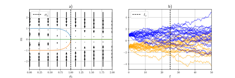
Figure 2: Visualization of a phase transition in a simple diffusion model (two deltas). a) Order parameter paths and (regularized) free energy gradients. The dashed line denotes the critical value of $\sigma_{t}=\sqrt{t}\sigma_{0}$. b) Forward process. The dashed line denotes time critical time.

Using our interpretation of $(t\sigma^{2})$ as a temperature parameter, we can define the Helmholtz free energy as follows

$$\mathcal{F}(\boldsymbol{x},t)=-(\sigma^{2}t)\log{Z(\boldsymbol{x},t)}~{}.$$ (15)

The expected value of the pattern $\boldsymbol{y}$ given $\boldsymbol{x}$ can then be expressed the gradient of the free energy with respect to $\boldsymbol{x}$:

$$\langle\boldsymbol{y}\rangle_{\boldsymbol{x}}=-\nabla\mathcal{F}(\boldsymbol{x},t)~{}.$$ (16)

This formula suggests an analogy between diffusion models and magnetic systems in statistical physics. The noisy state $\boldsymbol{x}$ can be interpreted as an external magnetic field, which induces the state of "magnetization" $\langle\boldsymbol{y}\rangle_{\boldsymbol{x}}$. In this analogy, a diffusion model is magnetized when its distribution is biased towards a sub-set of the possible microstates.

In physics, the ’external field’ variable $\boldsymbol{x}$ is usually assumed to be controlled by the experimenter. On the other hand, in generative diffusion models $\boldsymbol{x}$ is a dynamic variable that, under the reversed dynamics, is itself attracted towards $\langle\boldsymbol{y}\rangle_{\boldsymbol{x}}$ by the drift term:

$$\nabla\log{p_{t}(\boldsymbol{x})}\propto\left(\langle\boldsymbol{y}\rangle_{\boldsymbol{x}}-\boldsymbol{x}\right)$$ (17)

In other words, if we ignore the effect of the dispersion term, the state of the system is driven towards self-consistent points where $\boldsymbol{x}$ is equal to $\langle\boldsymbol{y}\rangle_{\boldsymbol{x}}$. In it therefore interesting to study the self-consistency equation

$$\boldsymbol{m}(\boldsymbol{h},t)=-\nabla\mathcal{F}(\boldsymbol{m}(\boldsymbol{h},t)+\boldsymbol{h},t)~{},$$ (18)

which defines the self-consistent solutions $\boldsymbol{m}(t)$ where the state is identical to the expected value. In the equation, we introduced a perturbation term $\boldsymbol{h}$, which will allow us to study how the systems react to perturbations. For $\boldsymbol{h}=0$, the equation can be equivalently re-expressed as the fixed point equation of the reversed drift:

$$\nabla\log{p_{t}(\boldsymbol{m}(\boldsymbol{0},t))}=\boldsymbol{0}~{}.$$ (19)

For $t\rightarrow\infty$, this equation admits the single "trivial" solution $\boldsymbol{m}=\langle\boldsymbol{y}\rangle_{0}$, where $\langle\cdot\rangle_{0}$ denotes expectation with respect to the target distribution $\phi(\boldsymbol{y})$. In analogy with magnetic systems, we can interpret $\boldsymbol{m}(\boldsymbol{h},t)$ as an order parameter and this equation as a thermodynamic equation of state. This analogy suggests that $\boldsymbol{m}(\boldsymbol{h},t)$ can be interpreted as a ’spontaneous magnetization’ of the system. From this point of view, we can conceptualize the generative process as a form of self.consistent spontaneous symmetry breaking on one of the many possible target points. In the following sections, we will formalize this insight by characterizing the critical behavior of this system.

Readers familiar with statistical physics will recognize that Eq. 18 is formally identical to the self-consistency conditions used in the mean field approximation, where the external field term in one location is assumed to be determined by the magnetization of all other locations. However, it is important to note that in the case of a diffusion model, this self-consistent coupling is not approximate, as it is a natural consequence of the dynamics. Nevertheless, the formal analogy implies that the thermodynamics of generative diffusion models is formally identical to the thermodynamics of mean field models.

4.1 The susceptibility matrix

In the physics of magnetic systems, the magnetic susceptibility matrix determines how much the different magnetization components are sensitive to the components of the external magnetic field. Similarly, in diffusion models we can define a susceptibility matrix:

$$\chi_{ij}(t)=\frac{\partial m_{i}}{\partial h_{j}}\bigg{\rvert}_{\boldsymbol{h}=0}~{},$$ (20)

which tells us how sensitive the expected value is to changes in the noisy-state $\boldsymbol{x}(t)$. The susceptibility matrix has a great value in interpreting the dynamics of the generative denoising process, as it informs us on how random fluctuations in each component of the state $\boldsymbol{x}(t)$ are propagated to the other components. For example, in the context of image generation, a random fluctuation of "green" at the bottom of an image will propagate to the rest, originating the image of a forest.

5 The regularized free energy

So far, we characterized the thermodynamic state of diffusion model at time $t$ by its Boltzmann distribution. The dynamics of the system can now be recovered as a form of (stochastic) free energy minimization:

$$\boldsymbol{x}(t-\text{d}t)=\boldsymbol{x}(t)-\frac{1}{t\sigma^{2}}\nabla\tilde{\mathcal{F}}(\boldsymbol{x},t)\text{d}t+\sigma\boldsymbol{w}(t)\sqrt{\text{d}t}~{},$$ (21)

where $\tilde{\mathcal{F}}$ is the free-energy plus a $L_{2}$ regularization term:

$$\tilde{\mathcal{F}}(\boldsymbol{x},t)=\mathcal{F}(\boldsymbol{x},t)+\frac{1}{2}{\left\lVert\boldsymbol{x}\right\rVert}_{2}^{2}$$ (22)

The symmetry breaking can now be detected as a change of shape in the regularized free energy, which transitions from a convex shape with a single global minimum to a more complex shape with potentially several meta-stable points (see Fig. 3). The reformulation of the dynamics in term of the gradient of a free energy allows us to interpret generative diffusion models as a kind of energy-based models (LeCun et al.,, 2006), as discussed in (Hoover et al.,, 2023) and (Ambrogioni,, 2023). The main difference is that the (free) energy is not learned directly but it is instead implicit in the learned score function. The connection suggests potential connection with the free energy principle in theoretical neuroscience, which is used to characterize the stochastic dynamics of biological neural systems (Friston,, 2010).

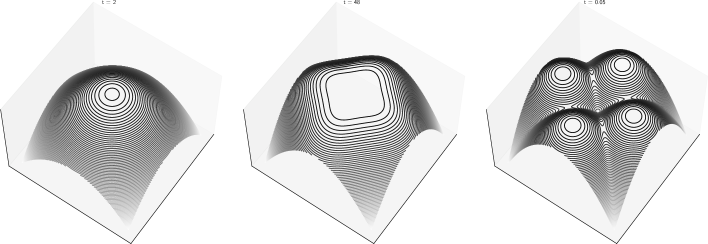
Figure 3: Negative free energy of a "four delta" 2d diffusion model for different values of the time variable. The target points are at $(1,0)$, $(0,1)$, $(-1,0)$ and $(0,-1)$.

6 Connecting the thermodynamics of diffusion models and physical systems: The diffused Ising model

While most of the formulas presented in this manuscript have a very close analogy with formulas in statistical physics, there are some subtle interpretative differences that could create confusion in the reader. To clarify these issues, we will discuss the diffused Ising model, which will provide a bridge between the two views. Consider a diffusion model with a target distribution supported on $d$-dimensional vectors $\boldsymbol{y}$ with entries in the set $\{-1,1\}$. The log-probability of the target distribution is defined by the following formula:

$$\log{\phi(\boldsymbol{y})}=-\frac{\beta}{2}\sum_{j\neq k}y_{j}y_{k}W_{jk}+c~{},$$ (23)

where W is a symmetric coupling matrix, $\beta$ is an inverse temperature parameter and $c$ is a constant. Up to constants, this is of course the log-probability of an Ising model without the external field term. From Eq. 7, up to constant terms, we obtain the following Hamiltonian for the diffusion model:

$$\mathcal{H}(\boldsymbol{y};\boldsymbol{x},t,\beta)=-(t\sigma^{2})^{-1}\boldsymbol{x}\cdot\boldsymbol{y}+\frac{\beta}{2}\sum_{j\neq k}y_{j}y_{k}W_{jk}~{},$$ (24)

which is almost identical to the Hamiltonian of an Ising model coupled to a location-dependent external field $\boldsymbol{x}$. Nevertheless, the quantity $t\sigma^{2}$, which we loosely interpreted as a "temperature", does not divide the coupling part of the Hamiltonian, which results in a radically different behavior. In fact, $t\sigma^{2}$ only modulates the susceptibility to the field term and it therefore does not radically alter the phase of the model, which depends on the parameter $\beta$. Instead, the interesting phase transition of the diffusion models is a consequence of the self-consistency relation in Eq. 18, which characterizes the branching of the fixed-points of the generative stochastic dynamics. From the point of view of statistical physics, Eq. 18 can be seen as the result of a mean-field approximation, where the average magnetization is coupled to the external field. However, it is important to keep in mind that, in a diffusion model, this mean-field approach does not represent the coupling between individual sites, which, as Eq. 24 shows, are instead statistically coupled by the interaction terms in the Hamiltonian. Instead, it can be seen as an idealized mean-field interaction between infinitely many copies of the whole system. In general, the value of $\beta$ will change the properties of the diffusion model, as the system transitions from its low temperature to its high temperature phase. The dependency of the diffusion dynamics on this transition have been extensively studied in Biroli and Mézard, (2023).

7 Phase transitions and symmetry breaking

A spontaneous symmetry breaking happens when this trivial solution for the order parameter branches into multiple solutions at some critical time of $t_{c}$. This corresponds to the onset of multi-modality in the regularized free energy $\tilde{\mathcal{F}}(\boldsymbol{x},t)$, as visualized in Fig. 3 for a "four deltas" model. In thermodynamic systems, the symmetry breaking corresponds to a (second order) phase transition, which in this case can be detected by the divergence of several state variables around the critical point.

The presence of one (or multiple) phase transitions in diffusion models depends on the target distribution $\phi(\boldsymbol{y})$. The simplest example is given by the "two deltas", which corresponds to the process visualized in Fig. 2 a. Using this distribution, we obtain the self-consistency equation

$$m=\tanh{\left(\frac{m}{t\sigma^{2}}\right)}$$ (25)

The solutions of this equation are shown in Fig. 2 b, together with the gradient of the regularized free energy, where we can see the branching of the solutions and the singular behavior around a critical point. Eq. 25 is identical to the mean-field self-consistency equation of an Ising model, from which we can deduce that the critical scaling of this simple generative diffusion moles shares its universality class. For example, by Taylor expansion of Eq.25 around $t_{c}=1$, we see that

$$m\sim(-\tau)^{1/2}$$ (26)

with $\tau=t-t_{c}$, which is valid for $t$ smaller than $t_{c}$.

7.1 Generation and critical instability

As shown in (Raya and Ambrogioni,, 2023), spontaneous symmetry breaking phenomena play a central role in the generative dynamics of diffusion models. Consider the simple "two deltas" model. For $t>>t_{c}$, the dynamics is mean-reverting towards a unique fixed-point $\boldsymbol{m}(\boldsymbol{0},t)$. Around $T=t_{c}$, the order parameter splits into thee "branches", an unstable one corresponding to the mean of the target distribution and two stable ones corresponding to the two target points. Importantly, at the critical point the susceptibility defined in Eq. 20 diverges, implying that the system becomes extremely reactive to fluctuations in the noise. This instability is determined by the critical exponents $\delta$ and $\gamma$ and , defined by the relations

$$h_{j}\propto m_{j}^{\delta_{j}}~{},$$ (27)

and

$$\chi_{ij}\propto(-\tau)^{\gamma_{ij}}~{}.$$ (28)

Note that, in the general case the critical exponents can be different for different coordinates and matrix entries. These divergences give rise to something we refer to as critical generative instability. We conjecture that the diversity of the generated samples crucially depends on a proper sampling of this critical region.

8 Studying the thermodynamics of trained diffusion models

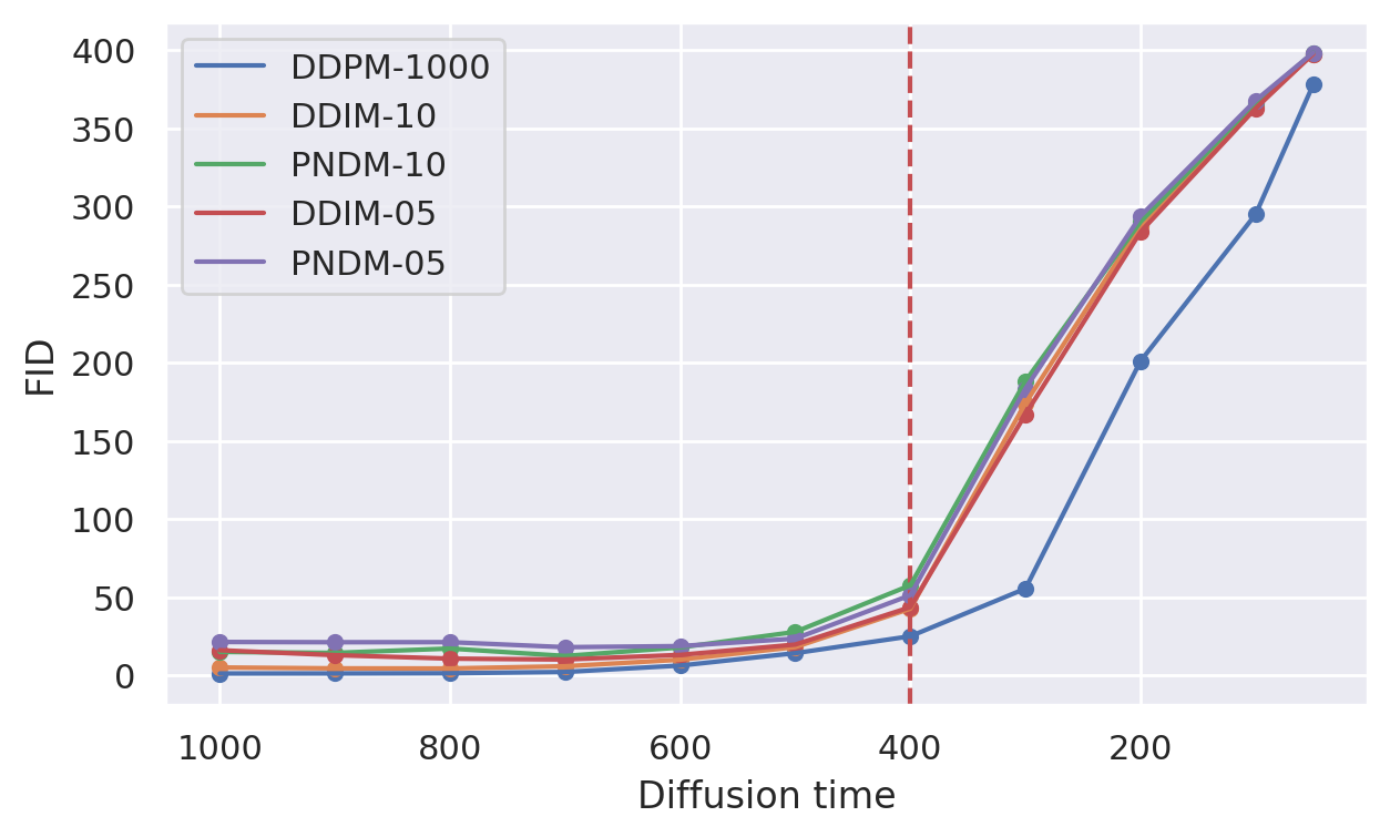
(a) MNIST

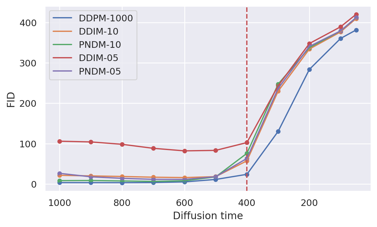
(b) CIFAR10

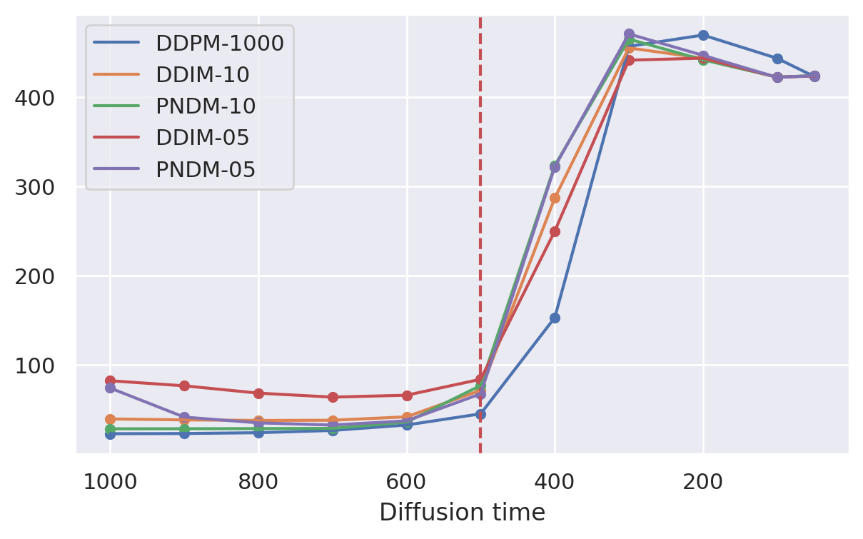
(c) Imagenet64

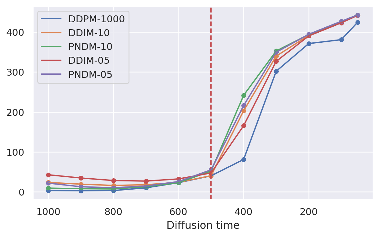
(d) CelebA64

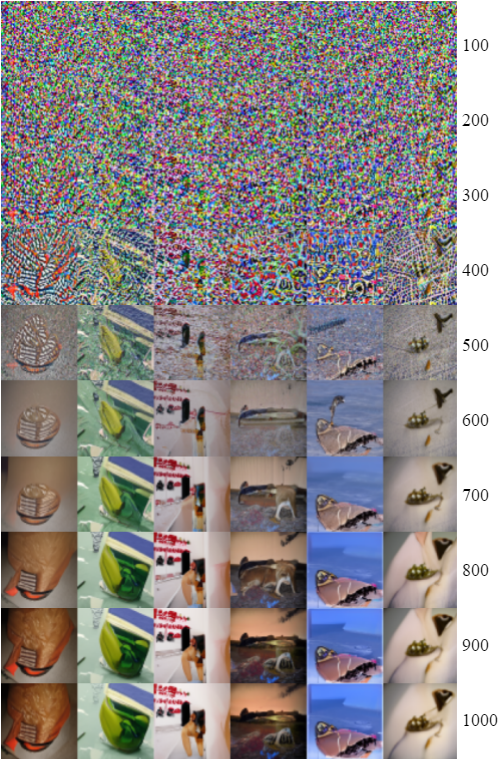
(e) Imagenet late start generation

Figure 4: Figure taken from (Raya and Ambrogioni,, 2023). Analysis of the model’s performance, as measured by FID scores, for different starting times using three different sampling methods: the normal DDPM sampler with decreasing time steps from $T=1000$ to 0, and fast sampler DDIM and PSDM for 10 and 5 denoising steps. The vertical line corresponds to the maximum of the second derivative of the FID curve, which offers a rough estimate of the first bifurcation time. (e) Illustrates samples generation on Imagenet64, while progressively varying the starting time from 1000 to 100.

In real-world applications, the target distribution $\phi(\boldsymbol{y})$ cannot be expressed in closed form. However, the thermodynamic properties of a trained diffusion model can be extracted from the optimized denoising network $\boldsymbol{f}^{*}(\boldsymbol{x}(t),t)$. For example, using Eq. 5 and Eq. 21, we can write the self-consistency equation in terms of the optimized denoising network:

$$\boldsymbol{f}^{*}(\boldsymbol{m}(\boldsymbol{h},t)+\boldsymbol{h},t)=\boldsymbol{h}~{},$$ (29)

which can be used to find the different solutions of the order parameter using numerical root-finding methods. However, the empirical study of the thermodynamics of trained models is complicated by the fact that, in general, the critical points are outside of the probable training range. This happens because, in high dimension, the distribution of the norm of $\boldsymbol{x}(t)$ concentrates on a fixed-variance shell around the fixed-points. In other words, while the fixed points are local maxima of the density, the region around them has very low probability since the noise tend to be equi-partitioned along all the degrees of freedom. This imply that the neighborhood of the order parameters are poorly trained, which leads to unreliable estimates when using Eq. 29. Conceptually, this suggests that the local scaling around the critical point is not important in itself, but it is instead important as it influences the shape of the free energy around the point.

9 Experimental evidence of phase transitions in trained diffusion models

The presence of one or more phase transitions in generative diffusion models is hard to prove for complex data distributions. However, symmetry breaking can be inferred experimentally from trained networks. For example, (Raya and Ambrogioni,, 2023) showed that the generative performance of models trained on images stay largely invariant when the reversed dynamics is initialized before $t_{\text{end}}$ up to a critical point (see Fig.4), as far as the system is initialized with a Gaussian with properly chosen mean vector and covariance matrix. This is consistent with out theoretical analysis since, prior to the first phase transition, the marginal distributions have a single global mode and are well approximated by normal distributions. As shown in the paper, the split in the free energy between different images can also be computed directly from trained networks. Together, these results suggest that generative diffusion models undergo a phase transition under most realistic data distributions.

10 Associative memory and Hopfield networks

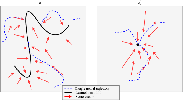
Figure 5: Visualization of the dynamics of a) a model trained as a generative model (semantic memory) and b) a model trained to retain an episodic memory.

Associative memory networks are energy-based learning systems that can store patterns (i.e. memories) as meta-stable states of a parameterized energy function (Hopfield,, 1982; Abu-Mostafa and Jacques,, 1985; Krotov,, 2023). There is a substantial literature on the thermodynamic properties of associative memory networks Strandburg et al., (1992); Volk, (1998); Marullo and Agliari, (2020). The original associative memory networks, also known as Hopfield networks are defined by the energy function $\mathcal{U}(\boldsymbol{x})=\frac{1}{2}\boldsymbol{x}^{T}W\boldsymbol{x}$ under the constraints of binary entries for the state vector. In a Hopfield network, a finite number of training patterns $\boldsymbol{y}_{j}$ are encoded into a weight matrix $W=\sum_{j}\boldsymbol{y}_{j}\boldsymbol{y}_{j}^{T}$, which usually gives the correct minima when the number of patterns is on the order of the dimensionality. Associative memory networks can reach much higher capacity by using exponential energy function (Krotov and Hopfield,, 2016; Demircigil et al.,, 2017; Krotov,, 2023). For example, (Ramsauer et al.,, 2021) introduces the use of the following function

$$\mathcal{U}(\boldsymbol{x})=-\beta^{-1}\log{\left(\sum_{j}e^{\beta\boldsymbol{x}\cdot\boldsymbol{y}_{j}}\right)}+\frac{1}{2}{\left\lVert\boldsymbol{x}\right\rVert}_{2}^{2}~{},$$ (30)

which can be proven to provide exponential scaling of the capacity and it is related to transformers architectures.

By inspection Eq. 30, we can see that this energy function is equivalent to the regularized Helmholtz free energy of a diffusion models trained on a mixture of delta distributions (see (Ambrogioni,, 2023) for more details): $\phi(\boldsymbol{y})=\sum_{j}\delta(\boldsymbol{y}-\boldsymbol{y}_{j})~{}.$ which gives a free energy with the same fixed-point structure of Eq. 30 at the zero temperature limit. Note that, while the dynamics of a diffusion model does not necessarily act as an optimizer in the general case, the free energy is exactly optimized when $\phi(\boldsymbol{y})$ is a sum of delta functions, making the dynamics of the model exactly equivalent to the optimization of Eq. 30 for $\beta\rightarrow\infty$. Given this connection, most of the results presented in this paper can be re-stated for associative memory networks. However, generative diffusion models are more general as they can target arbitrary mixtures of continuous and singular distributions, as visualized in Fig. 5.

11 Conclusions

In this paper, we presented a formulation of generative diffusion models in terms of equilibrium statistical mechanics. This allowed us to study the critical behavior of these generative models during second-order phase transitions. Our analysis establishes a deep connection between generative modeling and statistical physics, which may in the future allow physicists to study these machine learning models using the tools of computational and theoretical physics.

References

- Abu-Mostafa and Jacques, (1985) Abu-Mostafa, Y. and Jacques, J. S. (1985). Information capacity of the hopfield model. IEEE Transactions on Information Theory, 31(4):461–464.
- Ambrogioni, (2023) Ambrogioni, L. (2023). In search of dispersed memories: Generative diffusion models are associative memory networks. arXiv preprint arXiv:2309.17290.
- Anderson, (1982) Anderson, B. D. (1982). Reverse-time diffusion equation models. Stochastic Processes and their Applications, 12(3):313–326.
- Biroli and Mézard, (2023) Biroli, G. and Mézard, M. (2023). Generative diffusion in very large dimensions. arXiv preprint arXiv:2306.03518.
- Bond-Taylor et al., (2021) Bond-Taylor, S., Leach, A., Long, Y., and Willcocks, C. G. (2021). Deep generative modelling: A comparative review of vaes, gans, normalizing flows, energy-based and autoregressive models. IEEE transactions on pattern analysis and machine intelligence.
- Chen et al., (2020) Chen, N., Zhang, Y., Zen, H., Weiss, R. J., Norouzi, M., and Chan, W. (2020). Wavegrad: Estimating gradients for waveform generation. arXiv preprint arXiv:2009.00713.
- Demircigil et al., (2017) Demircigil, M., Heusel, J., Löwe, M., Upgang, S., and Vermet, F. (2017). On a model of associative memory with huge storage capacity. Journal of Statistical Physics, 168:288–299.
- Friston, (2010) Friston, K. (2010). The free-energy principle: a unified brain theory? Nature Reviews Neuroscience, 11(2):127–138.
- Ho et al., (2020) Ho, J., Jain, A., and Abbeel, P. (2020). Denoising diffusion probabilistic models. Advances in Neural Information Processing Systems.
- Ho et al., (2022) Ho, J., Salimans, T., Gritsenko, A., Chan, W., Norouzi, M., and Fleet, D. J. (2022). Video diffusion models. arXiv preprint arXiv:2204.03458.
- Hoover et al., (2023) Hoover, B., Strobelt, H., Krotov, D., Hoffman, J., Kira, Z., and Chau, H. (2023). Memory in plain sight: A survey of the uncanny resemblances between diffusion models and associative memories. arXiv preprint arXiv:2309.16750.
- Hopfield, (1982) Hopfield, J. J. (1982). Neural networks and physical systems with emergent collective computational abilities. Proceedings of the National Academy of Sciences, 79(8):2554–2558.
- Kong et al., (2020) Kong, Z., Ping, W., Huang, J., Zhao, K., and Catanzaro, B. (2020). Diffwave: A versatile diffusion model for audio synthesis. arXiv preprint arXiv:2009.09761.
- Krotov, (2023) Krotov, D. (2023). A new frontier for hopfield networks. Nature Reviews Physics, pages 1–2.
- Krotov and Hopfield, (2016) Krotov, D. and Hopfield, J. J. (2016). Dense associative memory for pattern recognition. Advances in Neural Information Processing Systems.
- LeCun et al., (2006) LeCun, Y., Chopra, S., Hadsell, R., Ranzato, M., and Huang, F. (2006). A tutorial on energy-based learning. Predicting structured data, 1(0).
- Liu et al., (2023) Liu, H., Chen, Z., Yuan, Y., Mei, X., Liu, X., Mandic, D., Wang, W., and Plumbley, M. D. (2023). Audioldm: Text-to-audio generation with latent diffusion models. arXiv preprint arXiv:2301.12503.
- Marullo and Agliari, (2020) Marullo, C. and Agliari, E. (2020). Boltzmann machines as generalized hopfield networks: a review of recent results and outlooks. Entropy, 23(1):34.
- Ramsauer et al., (2021) Ramsauer, H., Schäfl, B., Lehner, J., Seidl, P., Widrich, M., Adler, T., Gruber, L., Holzleitner, M., Pavlović, M., Sandve, G. K., et al. (2021). Hopfield networks is all you need. Internetional Conference on Learning Representations.
- Raya and Ambrogioni, (2023) Raya, G. and Ambrogioni, L. (2023). Spontaneous symmetry breaking in generative diffusion models. Neural Information Processing Systems.
- Singer et al., (2022) Singer, U., Polyak, A., Hayes, T., Yin, X., An, J., Zhang, S., Hu, Q., Yang, H., Ashual, O., Gafni, O., et al. (2022). Make-a-video: Text-to-video generation without text-video data. arXiv preprint arXiv:2209.14792.
- Sohl-Dickstein et al., (2015) Sohl-Dickstein, J., Weiss, E., Maheswaranathan, N., and Ganguli, S. (2015). Deep unsupervised learning using nonequilibrium thermodynamics. International Conference on Machine Learning.
- (23) Song, J., Meng, C., and Ermon, S. (2021a). Denoising diffusion implicit models. Internetional Conference on Learning Representations.
- (24) Song, Y., Sohl-Dickstein, J., Kingma, D. P., Kumar, A., Ermon, S., and Poole, B. (2021b). Score-based generative modeling through stochastic differential equations. In International Conference on Learning Representations.
- Strandburg et al., (1992) Strandburg, K. J., Peshkin, M. A., Boyd, D. F., Chambers, C., and O’Keefe, B. (1992). Phase transitions in dilute, locally connected neural networks. Physical Review A, 45(8):6135.
- Volk, (1998) Volk, D. (1998). On the phase transition of hopfield networks—another monte carlo study. International Journal of Modern Physics C, 9(05):693–700.