Bayesian Neural Controlled Differential Equations for Treatment Effect Estimation

Abstract

Treatment effect estimation in continuous time is crucial for personalized medicine. However, existing methods for this task are limited to point estimates of the potential outcomes, whereas uncertainty estimates have been ignored. Needless to say, uncertainty quantification is crucial for reliable decision-making in medical applications. To fill this gap, we propose a novel Bayesian neural controlled differential equation (BNCDE) for treatment effect estimation in continuous time. In our BNCDE, the time dimension is modeled through a coupled system of neural controlled differential equations and neural stochastic differential equations, where the neural stochastic differential equations allow for tractable variational Bayesian inference. Thereby, for an assigned sequence of treatments, our BNCDE provides meaningful posterior predictive distributions of the potential outcomes. To the best of our knowledge, ours is the first tailored neural method to provide uncertainty estimates of treatment effects in continuous time. As such, our method is of direct practical value for promoting reliable decision-making in medicine.

1 Introduction

Personalized medicine seeks to choose treatments that improve a patient’s future health trajectory. To this end, reliable estimates of treatment effects over time are needed (Allam et al., 2021; Bica et al., 2021). For example, in cancer therapy, a physician may base the decisions of applying chemotherapy on whether or not the expected health trajectory will improve after treatment.

In medicine, there is a growing interest in estimating treatment effects from patient trajectories using observational data (e.g., electronic health records) (Allam et al., 2021; Bica et al., 2021). Methods for this task should fulfill two requirements: (1) Existing methods typically require a patient’s health trajectory to be recorded in regular time steps (e.g., Bica et al., 2020; Melnychuk et al., 2022). However, medical practice is highly volatile and dynamic, as patients may need immediate treatment. Hence, methods are needed that model patient trajectories not in discrete time (e.g., fixed daily or hourly time steps) but in continuous time (i.e., actual timestamps). (2) To ensure reliable decision-making, medicine is not only interested in point estimates but also the corresponding uncertainty (e.g., credible intervals) (Zampieri et al., 2021). For example, rather than saying that a treatment is expected to reduce the size of a tumor by $x$, one is interested in whether the size of a tumor will reduce by $x$ with 95% probability, given the evidence of available data. Hence, methods for treatment effect estimation must allow for uncertainty quantification. To the best of our knowledge, a tailored method that accounts for both (1) and (2) is still missing.

Several neural methods have been developed for individualized treatment effect estimation from observational data over time (see Section 2 for an overview). Here, methods often focus on simplified settings in discrete time (e.g., Lim et al., 2018; Bica et al., 2020; Kuzmanovic et al., 2021; Li et al., 2021; Melnychuk et al., 2022) but not in continuous time. In contrast, there is only a single neural method that operates in continuous time, namely, TE-CDE (Seedat et al., 2022). Yet, this method lacks rigorous uncertainty quantification.

In this work, we develop a novel neural method for treatment effect estimation from observational data in continuous time that allows for Bayesian uncertainty quantification. For this purpose, we propose the Bayesian neural controlled differential equation (called BNCDE). In our BNCDE, we follow the Bayesian paradigm to account for both model uncertainty and outcome uncertainty. To the best of our knowledge, ours is the first tailored neural method for uncertainty-aware treatment effect estimation in continuous time.

In our BNCDE, the time dimension is modeled through a coupled system of neural controlled differential equations and neural stochastic differential equations, where the neural stochastic differential equations allow for tractable variational Bayesian inference. Specifically, we use latent neural SDEs to parameterize the posterior distribution of the weights in the neural controlled differential equations. By design, the solutions to our SDEs are stochastic weight processes based on which we then compute the Bayesian posterior predictive distribution of the potential outcomes in continuous time.

Our contributions are the following: (1) We develop a novel method for treatment effect estimation from observational data in continuous time with uncertainty quantification. (2) To the best of our knowledge, we are the first to propose a Bayesian version of neural controlled differential equations. (3) We show empirically that our method yields state-of-the-art performance.

2 Related Work

Continuous time Outcome uncertainty Model uncertainty RMSNs (Lim et al., 2018) ✗ ✗ ✗ CRN (Bica et al., 2020) ✗ ✗ ✗ G-Net (Li et al., 2021) ✗ ✓ (✗) CT (Melnychuk et al., 2022) ✗ ✗ ✗ TE-CDE (Seedat et al., 2022) ✓ ✗ (✗) BNCDE (ours) ✓ ✓ ✓ (✗):  Authors use only MC dropout for model uncertainty

Table 1: Overview of key neural methods for treatment effect estimation over time. Model uncertainty (epistemic) refers to the uncertainty with respect to the optimal model parameters. Outcome uncertainty (aleatoric) is the uncertainty that is inherent to the data-generating process. While model uncertainty decreases with increasing sample size, outcome uncertainty does not.

We discuss methods related to (i) individualized treatment effect estimation over time and (ii) neural ordinary differential equations, as well as Bayesian methods for (i) and (ii). Thereby, we show that a Bayesian method for uncertainty quantification in our setting is missing (see Table 1). We emphasize that we focus on methods for individualized treatment effect estimation over time and not for average treatment effect estimation (e.g. Robins et al., 2000; Robins & Hernán, 2009; Rytgaard et al., 2022; Frauen et al., 2023).

Treatment effect estimation over time: Many works focus on estimating heterogeneous treatment effects from observational data in the static setting (e.g., Johansson et al., 2016; Alaa & van der Schaar, 2017; Louizos et al., 2017; Shalit et al., 2017; Yoon et al., 2018; Zhang et al., 2020; Melnychuk et al., 2023a). In contrast, only a few works consider individualized treatment effect estimation in the dynamic setting, that is, over time. We focus on neural methods for this task, as existing non-parametric methods (Xu et al., 2016; Schulam & Saria, 2017; Soleimani et al., 2017) impose strong assumptions on the outcome distribution, are not designed for multi-dimensional outcomes and static covariate data, and scalability is limited.

(1) Some methods operate in discrete time. Examples are the recurrent marginal structural networks (RMSNs) (Lim et al., 2018), counterfactual recurrent network (CRN) (Bica et al., 2020), G-Net (Li et al., 2021), and causal transformer (CT) (Melnychuk et al., 2022). However, these methods are all limited to discrete time (e.g., regular recordings such as in daily or hourly time steps), which is often unrealistic in medical practice.

(2) A more realistic approach is to estimate treatment effects in continuous time. To the best of our knowledge, the only neural method for that purpose is the treatment effect neural controlled differential equation (TE-CDE) (Seedat et al., 2022). TE-CDE leverages neural controlled differential equations (CDEs) to capture treatment effects in continuous time (see Supplement A for details on TE-CDE). However, unlike our method, TE-CDE does not allow for uncertainty quantification.

In the continuous time setting, the timestamps of observation may be informative about the potential outcomes and bias their estimates. A general framework to address informative sampling has been developed in (Vanderschueren et al., 2023) and applied to TE-CDE. We later also apply this approach to our BNCDE; see Supplement H.

Uncertainty quantification for treatment effect estimation: Jesson et al. (2020) highlight the importance of Bayesian uncertainty quantification for treatment effect estimation in the static setting. In the time-varying setting, existing methods are limited in that they use Monte Carlo (MC) dropout (Gal & Ghahramani, 2016) as an ad-hoc solution. However, MC dropout relies upon mixtures of Dirac distributions in parameter space, which leads to approximations of the true posterior which are questionable and not faithful (Le Folgoc et al., 2021). In contrast, a tailored neural method for Bayesian uncertainty quantification in the continuous time setting is still missing.

Neural differential equations: Neural ordinary differential equations (ODEs) can be seen as infinitely-deep residual neural networks (Chen et al., 2018; Haber & Ruthotto, 2018; Lu et al., 2018), where infinitesimal small hidden layer transformations correspond to the dynamics of a time-evolving latent vector field. Neural CDEs (Kidger et al., 2020; Morrill et al., 2021) extend neural ODEs in order to process time series data in continuous time (for more details, see Supplement B).

Uncertainty quantification for neural ODEs: There are only a few existing approaches for this task. (1) Variants of Markov chain Monte Carlo (MCMC) have directly been applied to neural ODEs (Dandekar et al., 2022). However, MCMC methods are known to scale poorly to high dimensions. (2) Fast approximate Bayesian inference can be achieved through Laplace approximation (Ott et al., 2023). (3) $\text{ODE}^{2}$VAE (Yıldız et al., 2019) uses Gaussian distributions for variational inference in neural ODEs. Yet, both (2) and (3) rely on unimodal distributions with limited expressiveness. (4) The posterior can be approximated through neural stochastic differential equations (SDEs) (Li et al., 2020). A key benefit of this is that neural SDEs as a variational family are both scalable and arbitrarily expressive (Tzen & Raginsky, 2019; Xu et al., 2022). However, no work has integrated Bayesian uncertainty quantification into neural CDEs.

Research gap: As shown above, there is no method for treatment effect estimation in continuous time with Bayesian uncertainty quantification. To fill this gap, we propose our BNCDE. To the best of our knowledge, our BNCDE is also the first Bayesian neural CDE.

3 Problem Formulation

3.1 Setup

Let $t\in[0,\bar{T}]$ be the observation time and let $\tau\in(0,\Delta]$ be the prediction window. We then consider $n$ patients (i.i.d.) as realizations of the following variables: (1) Outcomes over time are given by $Y_{t}\in\mathbb{R}$ (e.g., tumor volume). (2) Covariates $X_{t}\in\mathbb{R}^{d_{x}}$ include additional patient information such as comorbidity. (3) Treatments are given by $A_{t}\in\{0,1\}^{d_{a}}$, where multiple treatments can be administered at the same time. The treatment assignment is controlled by a multivariate counting process $N_{t}\in\mathbb{N}_{0}^{d_{a}}$ with intensity $\lambda(t)$, where $N_{t}$ corresponds to the number of treatments assigned up to a specific point in time $t$. This is consistent with medical practice where the same treatment is oftentimes applied multiple times. For example, cancer patients may receive multiple cycles of chemotherapy (Curran et al., 2011).

Importantly, we focus on a setting in continuous time. That is, the outcomes and covariates of each patient $i$ are recorded at timestamps $\{t_{0}^{i},t_{1}^{i},\ldots,t_{m_{i}}^{i}\}$ with $t_{0}^{i}=0$ and $t_{m_{i}}^{i}=\bar{t}^{i}$, where $m_{i}$ is the number of timestamps and $\bar{t}^{i}$ is the latest observation time for patient $i$. This is a crucial difference from a setting in discrete time, since, in our setting, the timestamps are arbitrary and thus non-regular. Further, the timestamps may differ between patients.

We have access to observational data $h_{t}^{i}=\{y_{[0,t]}^{i},x_{[0,t]}^{i},a_{[0,t]}^{i}\}$, $t\in[0,\bar{t}^{i}]$, which we refer to as patient trajectories. Formally, the observed outcomes at time $t$ are given by $y_{[0,t]}^{i}=\bigcup_{\ell\leq k_{i}}\{y_{t_{\ell}^{i}}^{i}\}$ and the observed covariates by $x_{[0,t]}^{i}=\bigcup_{\ell\leq k_{i}}\{x_{t_{\ell}^{i}}^{i}\}$, where $t_{k_{i}}^{i}\leq t$ is the latest observation time up to time $t$ with $k_{i}\leq m_{i}$. In contrast, we have full knowledge of the history of assigned treatments, i.e., ${a^{i}_{[0,t]}=\bigcup_{s\leq t}\{a_{s}^{i}\}}$. We are interested in the potential outcome for a new patient $*$ at time $\bar{t}^{*}+\Delta$, $Y_{\bar{t}^{*}+\Delta}[a_{(\bar{t}^{*},\bar{t}^{*}+\Delta]}^{\prime}]$, for an arbitrary future sequence of treatments $a_{(\bar{t}^{*},\bar{t}^{*}+\Delta]}^{\prime}=\bigcup_{\bar{t}^{*}<\tau\leq\bar{t}^{*}+\Delta}a_{\tau}^{\prime}$, given a patient’s observed trajectory ${h}_{\bar{t}^{*}}^{*}$. For notation, we write $h_{(\bar{t}^{i}+\Delta)^{-}}^{i}=h_{\bar{t}^{i}}^{i}\cup\{a_{(\bar{t}^{i},\bar{t}^{i}+\Delta]}^{i}\}$ when we include the factual future sequence of treatments. We write $h_{\bar{t}^{i}+\Delta}^{i}=h_{(\bar{t}^{i}+\Delta)^{-}}^{i}\cup\{y_{\bar{t}^{i}+\Delta}^{i}\}$ when we further include the realized observed outcome for this future sequence of treatments.

3.2 Estimation Task

Our objective is to predict the potential outcome for a future sequence of assigned treatments, given the observed patient history. In the following, we adopt the potential outcomes framework (Neyman, 1923; Rubin, 1978) and its extensions to the time-varying setting (Lok, 2008; Robins & Hernán, 2009; Saarela & Liu, 2016; Rytgaard et al., 2022).

Unique to our setting is that we do not focus on simple point estimates but perform Bayesian uncertainty quantification. In the Bayesian framework, model parameters $\omega\in\Omega$ are assigned a prior distribution $p(\omega)$. Further, for an individual $*$ and a future sequence of treatments $a_{(\bar{t}^{*},\bar{t}^{*}+\Delta]}^{\prime}$, the potential outcome $Y_{\bar{t}^{*}+\Delta}[a_{(\bar{t}^{*},\bar{t}^{*}+\Delta]}^{\prime}]$ has a likelihood $p(Y_{\bar{t}^{*}+\Delta}[a_{(\bar{t}^{*},\bar{t}^{*}+\Delta]}^{\prime}]\mid h_{\bar{t}^{*}}^{*},\omega)$, given a parameter realization $\omega$ and patient trajectory $h_{\bar{t}^{*}}^{*}$. We thus aim to estimate the posterior predictive distribution

$$p(Y_{\bar{t}^{*}+\Delta}[a_{(\bar{t}^{*},\bar{t}^{*}+\Delta]}^{\prime}]\mid h_{\bar{t}^{*}}^{*},\mathcal{H})=\mathbb{E}_{p(\omega\mid\mathcal{H})}\left[p(Y_{\bar{t}^{*}+\Delta}[a_{(\bar{t}^{*},\bar{t}^{*}+\Delta]}^{\prime}]\mid h_{\bar{t}^{*}}^{*},\omega)\right],$$ (1)

which is the weighted average likelihood under the parameter posterior distribution $p(\omega\mid\mathcal{H})$ given the training data $\mathcal{H}=\bigcup_{i=1}^{n}h_{\bar{t}^{i}+\Delta}^{i}$. Of note, our setting is different from other works such as TE-CDE (Seedat et al., 2022), where only point estimates such as $\mathbb{E}[Y_{\bar{t}^{*}+\Delta}[a_{(\bar{t}^{*},\bar{t}^{*}+\Delta]}^{\prime}]\mid h_{\bar{t}^{*}}^{*}]$ are computed but without uncertainty quantification. Instead, we estimate the full distribution of the potential outcomes.

3.3 Identifiability

The above estimation task is challenging due to the fundamental problem of causal inference (Imbens & Rubin, 2015) in that only factual but never counterfactual patient trajectories are observed. To ensure identifiability from observational data, we make the following three assumptions that are standard in the literature (Lok, 2008; Robins & Hernán, 2009; Saarela & Liu, 2016; Rytgaard et al., 2022): (1) Consistency: Given a sequence of treatments $A_{[0,t+\tau]}=a_{[0,t+\tau]}$, $t\geq 0$ and $\tau\in[0,\Delta]$, the potential outcome $Y_{t+\tau}[a_{[0,t+\tau]}]$ coincides with the observed outcome $Y_{t+\tau}$. (2) Overlap: For any realization of patient history $H_{t}=h_{t}$, there is a positive probability of receiving treatment at any point $t$ in time. That is, the intensity process satisfies $0<\lambda(t\mid h_{t})<1$. (3) Unconfoundedness: The treatment assignment probability is independent of future outcomes and unobserved information. This means that the intensity process satisfies $\lambda(t\mid h_{t})=\lambda(t\mid h_{t},\mathcal{F}(Y_{s}[a^{\prime}_{(t,s]}]:s>t))$, where $\mathcal{F}(Y_{s}[a^{\prime}_{(t,s]}]:s>t)$ is the filtration generated by future potential outcomes.

4 Bayesian neural controlled differential equation

4.1 Architecture

Figure 1: Our BNCDE consists of an encoder, a decoder, and a prediction head.

Our BNCDE builds upon an encoder-decoder architecture (see Figure 1) with three components. The  encoder receives the patient trajectory $H_{t}$ in continuous time and encodes it into a hidden representation $Z_{t}$ up to time $\bar{T}$. The  decoder then takes the hidden representation $Z_{\bar{T}}$ together with a future sequence of treatments $a_{\tau}^{\prime}$ and transforms it into a new hidden representation $\tilde{Z}_{\tau}$ for $0<\tau\leq\Delta$, where $\Delta$ is the desired prediction window. Both the encoder and the decoder each consist of (i) a neural CDE and (ii) a latent neural SDE. (i) The neural CDEs compute hidden representations of the patient trajectories in continuous time. (ii) The latent neural SDEs approximate the posterior distribution of the neural CDE weights. Finally, the  prediction head receives $\tilde{Z}_{\Delta}$ and parameterizes the likelihood of the potential outcome. We explain the different components in the following.

Encoder: The encoder has two components, namely a neural CDE and a latent neural SDE: (i) The neural CDE encodes a hidden representation that is driven by the patient history. (ii) The latent neural SDE approximates the posterior distribution of the neural CDE weights.

The neural CDE consists of a trainable embedding network $\eta_{\phi}^{e}:\mathbb{R}^{1+d_{x}+d_{a}}\to\mathbb{R}^{d_{z}}$ that encodes the initial outcome $Y_{0}$, covariates $X_{0}$, and treatments $A_{0}$ into a hidden state $Z_{0}$. The hidden state $Z_{0}$ serves as the initial condition of the neural CDE. Formally, it is given by

$$Z_{t}=\int_{0}^{t}f^{e}(Z_{s},s\mid\omega_{s})\mathop{}\!\mathrm{d}[Y_{s},X_{s},A_{s}],\quad t\in(0,\bar{T}],\quad Z_{0}=\eta_{\phi}^{e}(Y_{0},X_{0},A_{0}),$$ (2)

where $f^{e}(Z_{t},t\mid\omega_{t}):\mathbb{R}^{d_{z}+1}\to\mathbb{R}^{d_{z}\times(1+d_{x}+d_{a})}$ is the neural vector field controlled by $[Y_{t},X_{t},A_{t}]$ given the network weights $\omega_{t}$. In particular, $f^{e}$ is a Bayesian neural network. It encodes information about the patient patient history into the hidden states $Z_{t}$ at any time $t\in[0,\bar{T}]$. Given the observed data, the posterior distribution of the random weights $\omega_{t}$ is modeled through the latent neural SDE. Hence, the weights are not static but time-varying. The output $Z_{\bar{T}}$ is then passed to the decoder.

The neural SDE is used to model the neural CDE weights $\omega_{t}\in\mathbb{R}^{d_{\omega}}$. Here, we assume that the weights evolve over time according to a stochastic process, where the stochastic process is the solution to the latent neural SDE. Specifically, we optimize the neural SDE to approximate the joint posterior distribution $p(\omega_{[0,\bar{T}]}\mid\mathcal{H})$ of the weights $\omega_{t}$ on $[0,\bar{T}]$ given the training data. We refer to the joint variational distribution as $q_{\phi}^{e}(\omega_{[0,\bar{T}]})$. Then, the neural SDE is formally defined by

$$\omega_{t}=\int_{0}^{t}g_{\phi}^{e}(\omega_{s},s)\mathop{}\!\mathrm{d}s+\int_{0}^{t}\sigma\mathop{}\!\mathrm{d}B_{s},\quad t\in(0,\bar{T}],\quad\omega_{0}=\xi_{\phi}^{e},$$ (3)

where $g_{\phi}^{e}:\mathbb{R}^{d_{\omega}+1}\to\mathbb{R}^{d_{\omega}}$ is the drift network, $\sigma$ is a constant diffusion coefficient, $B_{t}\in\mathbb{R}^{d_{\omega}}$ is a standard Brownian motion, and $\xi_{\phi}^{e}\sim\mathcal{N}(\nu_{\phi}^{e},\sigma)$ is the initial condition.

Decoder: The decoder also consists of a neural CDE and a latent neural SDE. (i) The neural CDE is controlled by a future sequence of treatments. (ii) The latent neural SDE approximates the posterior distribution of the neural CDE weights.

The neural CDE takes the hidden representation $Z_{\bar{T}}$ from the encoder as the initial condition. The neural CDE is then given by

$$\tilde{Z}_{\tau}=\int_{0}^{\tau}f^{d}(\tilde{Z}_{s},s\mid\tilde{\omega}_{s})\mathop{}\!\mathrm{d}a_{s}^{\prime},\quad\tau\in(0,\Delta],\quad\tilde{Z}_{0}=Z_{\bar{T}},$$ (4)

where $f^{d}(\tilde{Z}_{\tau},\tau\mid\tilde{\omega}_{\tau}):\mathbb{R}^{d_{z}+1}\to\mathbb{R}^{d_{z}\times(1+d_{x}+d_{a})}$ is the Bayesian neural vector field controlled by a future sequence of treatments $a_{\tau}^{\prime}$ given the network weights $\tilde{\omega}_{\tau}$. The hidden state $\tilde{Z}_{\Delta}$ is then passed to the prediction head.

The neural SDE is defined in the same way as in the encoder. It is used to make a variational approximation $q_{\phi}^{d}(\tilde{\omega}_{[0,\Delta]})$ of the joint posterior distribution $p(\tilde{\omega}_{[0,\Delta]}\mid\mathcal{H},\omega_{[0,\bar{T}]})$ of the weights $\tilde{\omega}_{\tau}$ on $[0,\Delta]$ given the training data and the neural CDE weights from the encoder. Formally, the neural SDE is given by

$$\tilde{\omega}_{\tau}=\int_{0}^{\tau}g_{\phi}^{d}(\tilde{\omega}_{s},s)\mathop{}\!\mathrm{d}s+\int_{0}^{\tau}\sigma\mathop{}\!\mathrm{d}\tilde{B}_{s},\quad\tau\in(0,\Delta],\quad\tilde{\omega}_{0}=\xi_{\phi},$$ (5)

where $g_{\phi}^{d}:\mathbb{R}^{d_{\tilde{\omega}}+1}\to\mathbb{R}^{d_{\tilde{\omega}}}$ is the drift network, $\tilde{B}_{\tau}\in\mathbb{R}^{d_{\tilde{\omega}}}$ is another standard Brownian motion, and $\xi_{\phi}^{d}\sim\mathcal{N}(\nu_{\phi}^{d},\sigma)$ is the initial condition.

Prediction head: The prediction head is a trainable mapping $\eta_{\phi}^{p}:\mathbb{R}^{d_{z}}\to\mathbb{R}^{2}$. It takes the hidden state $\tilde{Z}_{\Delta}$ as input and then predicts the expected value $\mu_{\bar{T}+\Delta}$ and the outcome uncertainty $\Sigma_{\bar{T}+\Delta}$ of the potential outcome at time $\bar{T}+\Delta$ via

$$(\mu_{\bar{T}+\Delta},\Sigma_{\bar{T}+\Delta})=\eta_{\phi}^{p}(\tilde{Z}_{\Delta}).$$ (6)

4.2 Coupled System of Neural Differential Equations

We can write our BNCDE as a coupled system of differential equations, which allows our BNCDE to learn in an end-to-end manner. Formally, the system of neural differential equations is given by

$$\mathop{}\!\mathrm{d}\begin{pmatrix}\tilde{\omega}_{\tau}\\[3.0pt] \tilde{Z}_{\tau}\\[3.0pt] \end{pmatrix} =\begin{pmatrix}g_{\phi}^{d}(\tilde{\omega}_{\tau},{\tau})\\[3.0pt] f^{d}(\tilde{Z}_{\tau},\tau\mid\tilde{\omega}_{\tau})\\[3.0pt] \end{pmatrix}\mathop{}\!\mathrm{d}\begin{pmatrix}\tau\\[3.0pt] a_{\tau}^{\prime}\\[3.0pt] \end{pmatrix}+\sigma\mathop{}\!\mathrm{d}\begin{pmatrix}\tilde{B}_{\tau}\\[3.0pt] 0\\[3.0pt] \end{pmatrix},$$ (7)

$$\mathop{}\!\mathrm{d}\begin{pmatrix}\omega_{t}\\[3.0pt] Z_{t}\\[3.0pt] \end{pmatrix} =\begin{pmatrix}g_{\phi}^{e}(\omega_{t},t)\\[3.0pt] f^{e}(Z_{t},t\mid\omega_{t})\\[3.0pt] \end{pmatrix}\mathop{}\!\mathrm{d}\begin{pmatrix}t\\[3.0pt] [Y_{t},X_{t},A_{t}]\\[3.0pt] \end{pmatrix}+\sigma\mathop{}\!\mathrm{d}\begin{pmatrix}B_{t}\\[3.0pt] 0\\[3.0pt] \end{pmatrix},$$ (8)

with initial conditions

$$\tilde{Z}_{0}=Z_{\bar{T}},\quad\tilde{\omega}_{0}=\xi_{\phi}^{d},\quad Z_{0}=\eta_{\phi}^{e}(Y_{0},X_{0},A_{0})\quad\text{and}\quad\omega_{0}=\xi_{\phi}^{e},$$ (9)

and where $t\in(0,\bar{T}]$ and $\tau\in(0,\Delta]$. The prediction head then outputs $(\mu_{\bar{T}+\Delta},\Sigma_{\bar{T}+\Delta})=\eta_{\phi}^{p}(\tilde{Z}_{\Delta})$. The embedding network $\eta_{\phi}^{e}$, the prediction head $\eta_{\phi}^{p}$, the initial conditions $\xi_{\phi}^{e}$ and $\xi_{\phi}^{d}$, and the drift networks $g_{\phi}^{e}$ and $g_{\phi}^{d}$ are learned via gradient-based methods.

For our model, the use of neural SDEs has three main benefits. (1) Neural SDEs allow us to approximate parameter posterior distributions that are arbitrarily complex. We emphasize that, although $\sigma$ is constant, prior research (Tzen & Raginsky, 2019; Xu et al., 2022) shows that given a sufficiently expressive family of drift networks, neural SDEs are able to approximate the true posterior distributions with arbitrary accuracy. (2) Our neural SDEs are non-autonomous, which means that they directly incorporate dependency on time. This way, we make sure that the weights learn to adjust their dynamics over time. (3) Our neural SDEs are learned through variational inference, which allows for optimization with gradient-based methods and is thus scalable.

4.3 Posterior Predictive Distribution

Our model generates the full posterior predictive distribution of the potential outcome, given patient history and training data. For a potential outcome at time $\bar{t}^{*}+\Delta$, our variational approximation of the posterior predictive distribution in Eq. 1 is given by

$$\mathbb{E}_{p(\tilde{\omega}_{[0,\Delta]},\omega_{[0,\bar{t}^{*}]}\mid\mathcal{H})}\left[p(Y_{\bar{t}^{*}+\Delta}[a_{(\bar{t}^{*},\bar{t}^{*}+\Delta]}^{\prime}]\mid\tilde{\omega}_{[0,\Delta]},\omega_{[0,\bar{t}^{*}]},h_{\bar{t}^{*}}^{*})\right]$$

$$\approx\mathbb{E}_{q_{\phi}^{e}(\omega_{[0,\bar{t}^{*}]})}\Big{\{}\mathbb{E}_{q_{\phi}^{d}(\tilde{\omega}_{[0,\Delta]})}\left[p(Y_{\bar{t}^{*}+\Delta}[a_{(\bar{t}^{*},\bar{t}^{*}+\Delta]}^{\prime}]\mid\tilde{\omega}_{[0,\Delta]},\omega_{[0,\bar{t}^{*}]},h_{\bar{t}^{*}}^{*})\right]\Big{\}}.$$ (10)

Hence, our posterior predictive distribution can be thought of as a Gaussian mixture model with infinitely many mixture components parameterized by the weights $\omega_{[0,\bar{T}^{*}]}$ and $\tilde{\omega}_{[0,\Delta]}$. We provide a formal derivation in Supplement D.

We emphasize that our model incorporates both (1) model uncertainty (epistemic) and (2) outcome uncertainty (aleatoric): (1) Model uncertainty is represented by the variance of the latent neural SDEs. The variances of the marginals $q_{\phi}^{e}(\omega_{t})$ and $q_{\phi}^{d}(\omega_{\tau})$ are larger for patient histories $h_{\bar{t}^{*}}^{*}$ and future sequences of treatments $a_{(\bar{t}^{*},\bar{t}^{*}+\Delta]}^{\prime}$ that are unlike any observations in the training data $\mathcal{H}$. Correspondingly, this leads to a larger variance of the posterior predictive distribution. Our BNCDE therefore informs about uncertainty in predictions due to lack of data support. (2) Outcome uncertainty is determined by the likelihood variance $\Sigma_{\bar{t}^{*}+\Delta}$. A larger likelihood variance implies that for a given patient history $h_{\bar{t}^{*}}^{*}$ and a future sequence of treatments $a_{(\bar{t}^{*},\bar{t}^{*}+\Delta]}^{\prime}$, there is a higher degree of variability in the potential outcome at future time $\bar{t}^{*}+\Delta$.

4.4 Training

Our BNCDE is trained by maximizing the evidence lower bound (ELBO), which further requires the specification of prior distributions of the neural CDE weights and a likelihood.

Priors: Our chosen priors for both the encoder weights $\omega_{t}$ and the decoder weights $\tilde{\omega}_{\tau}$ are independent Ornstein-Uhlenbeck (OU) processes due to their finite variance in the time limit. We set the prior drifts to $h^{e}(\omega_{t})=(-\omega_{t})$ and $h^{d}(\tilde{\omega}_{\tau})=(-\tilde{\omega}_{\tau})$ respectively and the diffusion coefficients to $\sigma$.

Likelihood: The likelihood in Eq. 10 is a normal distribution parameterized by the prediction head in Eq. 6. That is, we model the likelihood as

$$Y_{\bar{T}+\Delta}[a_{(\bar{T},\bar{T}+\Delta]}^{\prime}]\mid(\tilde{\omega}_{[0,\Delta]},\omega_{[0,\bar{T}]},H_{\bar{T}})\sim\mathcal{N}(\mu_{\bar{T}+\Delta},\Sigma_{\bar{T}+\Delta}).$$ (11)

ELBO: For training, we optimize the variational posterior distribution of the weights using the data $\mathcal{H}$. Specifically, we the maximize ELBO for an observation $i$ given by

$$\log p(y_{\bar{t}^{i}+\Delta}^{i}\mid h_{(\bar{t}^{i}+\Delta)^{-}}^{i})\geq \mathbb{E}_{q_{\phi}^{e}(\omega_{[0,\bar{t}^{i}]})}\Big{\{}\mathbb{E}_{q_{\phi}^{d}(\tilde{\omega}_{[0,\Delta]})}\Big{[}\log p(y_{\bar{t}^{i}+\Delta}^{i}\mid\tilde{\omega}_{[0,\Delta]},\omega_{[0,\bar{t}^{i}]},h_{(\bar{t}^{i}+\Delta)^{-}}^{i})\Big{]}\Big{\}}$$

$$-D_{\mathrm{KL}}[q_{\phi}^{d}(\tilde{\omega}_{[0,\Delta]})\;\|\;p(\tilde{\omega}_{[0,\Delta]})]-D_{\mathrm{KL}}[q_{\phi}^{e}(\omega_{[0,\bar{t}^{i}]})\;\|\;p(\omega_{[0,\bar{t}^{i}]})],$$ (12)

where $D_{\text{KL}}$ is the Kullback–Leibler divergence, $p(\tilde{\omega}_{[0,\Delta]})$ and $p(\omega_{[0,\bar{t}^{i}]})$ are the joint distributions of the OU priors on $[0,\Delta]$ and $[0,\bar{t}^{i}]$ respectively. We provide a full derivation of the ELBO loss in Supplement D. A summary of the numerical ELBO approximation is provided in Supplement E. Further implementation details of our model are provided in Supplement F.

5 Numerical Experiments

5.1 Setup

Data: We benchmark our method using the established pharmacokinetic-pharmacodynamic tumor growth model by Geng et al. (2017). Variants of this model are the standard used to assess the performance of time-varying treatment effect models (Lim et al., 2018; Bica et al., 2020; Li et al., 2021; Melnychuk et al., 2022; Seedat et al., 2022; Vanderschueren et al., 2023). In the tumor growth model, the outcome $Y_{t}$ is the tumor volume, which evolves according to the differential equation

$${\mathop{}\!\mathrm{d}Y_{t}}=\bigg{[}1+\underbrace{\rho\log\left(\frac{K}{Y_{t}}\right)}_{\text{Tumor growth}}-\underbrace{\alpha_{c}c_{t}}_{\text{Chemotherapy}}-\underbrace{(\alpha_{r}d_{t}+\beta_{r}d_{t}^{2})}_{\text{Radiotherapy}}+\underbrace{\epsilon_{t}}_{\text{Noise}}\bigg{]}Y_{t}\mathop{}\!\mathrm{d}t,$$ (13)

where the coefficients $\rho,K,\alpha_{c}\alpha_{r},\beta_{r},\epsilon_{t}$ are sampled as in Geng et al. (2017). At time $t$, a treatment may be applied and, if so, includes chemotherapy, radiotherapy, or both. We employ the same model variant as in Vanderschueren et al. (2023), where observations are sampled non-regularly, that is, in continuous time. We provide more details in Supplement C.

Baselines: Due to the novelty of our setting, there are no existing baselines for uncertainty quantification in continuous time (see Table 1). The only comparable method is TE-CDE with Monte Carlo (MC) dropout (Seedat et al., 2022). Implementation details are in Supplement F.

Performance metrics: We use different metrics to assess whether the uncertainty estimates of our method are faithful and sharp. To this end, we examine the predictive posterior credible intervals (CrIs) of the potential outcomes generated by the different methods. For each patient, we compute the individual equal-tailed $(1-\alpha)$ posterior predictive CrI with $\alpha\in[0.01,0.05]$. This choice is motivated by medical practice, where the treatment effectiveness is typically evaluated based on the 95% and 99% CrIs. We assess the faithfulness of the CrIs by computing the empirical coverage, that is, the proportion of times the CrIs contain the outcomes in the test data. We further assess the sharpness of the computed CrIs by reporting the median width of the CrIs between 95% and 99% over all patients in the test data. We report the results for the prediction windows ${\Delta=1,2,3}$. Results for additional prediction windows in Supplement G. We report the averaged results along with the standard deviation over five different seeds.

We further evaluate the error in the point estimates. Specifically, we compute the mean squared error (MSE) of the Monte Carlo mean estimates of the observed outcomes.

5.2 Results

$\blacksquare$ Faithfulness: We first evaluate whether the estimated CrIs are faithful. For this, we show the empirical coverage across different quantiles $(1-\alpha)$. The results are in Fig. 2. For our BNCDE, the $(1-\alpha)$ CrI almost always contains at least $(1-\alpha)$ of the outcome, implying that the estimated CrIs are generally faithful. In contrast, the estimated CrIs for TE-CDE are generally not faithful. In particular, the CrIs from TE-CDE often contain fewer outcomes than the $(1-\alpha)$ level should guarantee, implying that the uncertainty estimates from TE-CDE are overconfident. This is in line with the literature, where MC dropout is found to produce poor approximations of the posterior (Le Folgoc et al., 2021). For longer prediction windows $\Delta$, the advantages from our method are even greater. In sum, the results demonstrate that our method is clearly superior.

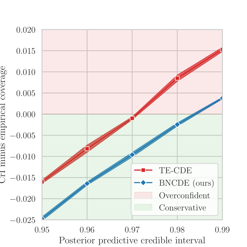
(a) $\Delta=1$

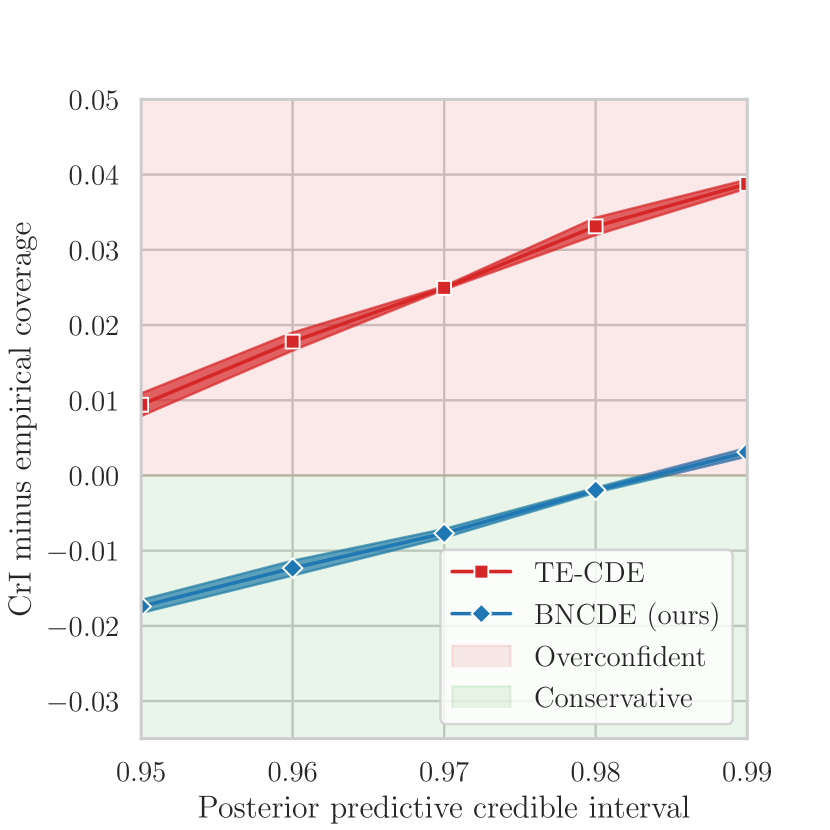
(b) $\Delta=2$

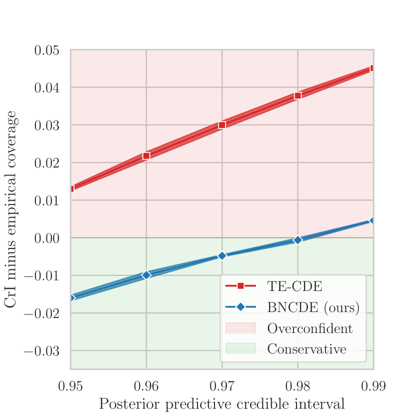
(c) $\Delta=3$

Figure 2: Faithfulness: Empirical coverage across different CrI quantiles. Shown are different prediction windows $\Delta=1,2,3$. Areas in green (red) indicate that the CrIs are faithful (not faithful).

$\blacksquare$ Sharpness: We compare the median width of estimated CrIs (see Figure 3). The CrIs from our BNCDE are significantly sharper than those of TE-CDE. This holds for all prediction windows, which further demonstrates the effectiveness of our method.

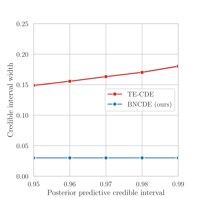
(a) $\Delta=1$

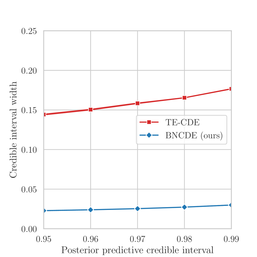
(b) $\Delta=2$

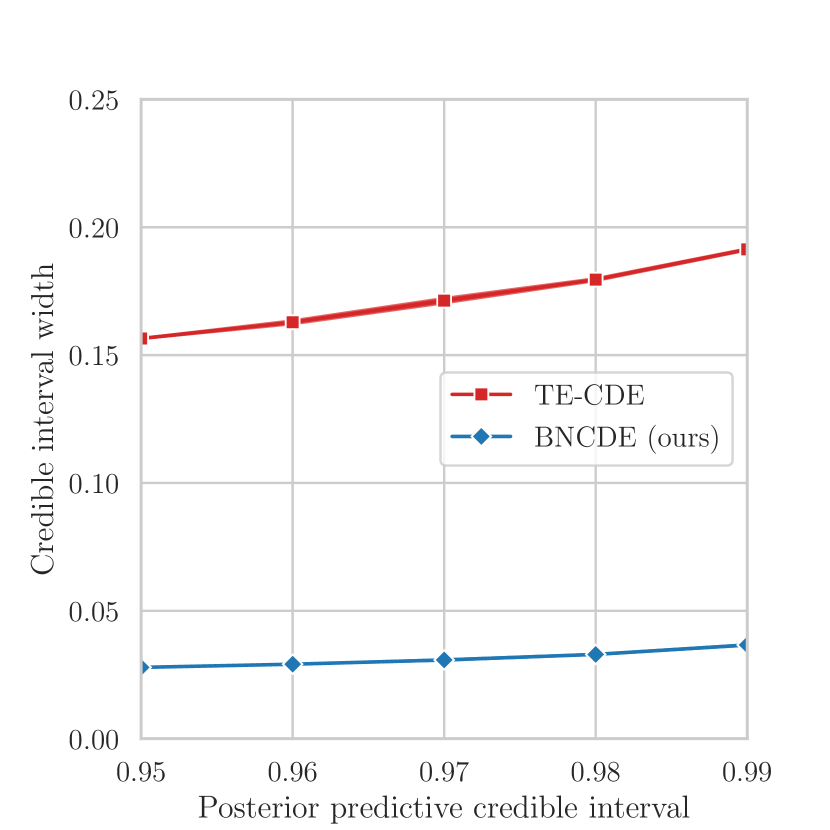
(c) $\Delta=3$

Figure 3: Sharpness: Width of the CrIs (median) for different quantiles $\alpha$.

$\blacksquare$ Error in point estimates: We further compare the errors in the Monte Carlo mean estimates of the treatment effects. The rationale is that our BNCDE may be better at computing the posterior distribution, yet the more complex architecture could hypothetically let the point estimates deteriorate. However, this is not the case, and we see that our BNCDE is clearly superior (see Fig. 4). We further find that the performance gain from our method is robust across different levels of noise in the data-generating process (i.e., larger $\text{Var}(\epsilon_{t})$).

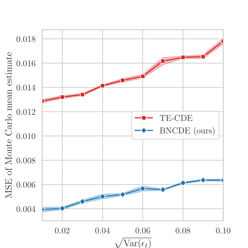
(a) $\Delta=1$

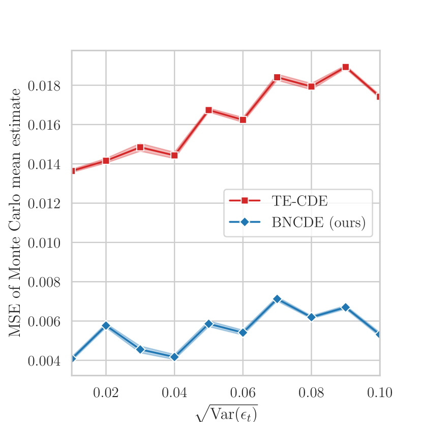
(b) $\Delta=2$

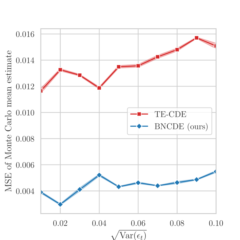
(c) $\Delta=3$

Figure 4: Error in point estimates: Reported is the median over the mean squared errors (MSE) of the point estimates of the outcomes. The results are based on test data that is generated with varying levels of noise, i.e., $\text{Var}(\epsilon_{t})$.

5.3 Comparison of Model Uncertainty

We now provide a deep-dive comparing the uncertainty estimates for model uncertainty only (and thus without outcome uncertainty). We do so for two reasons: (1) We can directly compare the model uncertainty from both our BNCDE and TE-CDE with MC dropout as the latter is limited to model uncertainty. (2) We can better understand the role of the neural SDE in our method (i.e., before the variational approximations are passed to the prediction head). For TE-CDE, we thus use the variance in the MC dropout samples as a measure of model uncertainty. For our BNCDE, we capture the model uncertainty with the Monte Carlo variance in the means of the likelihood $\mu_{\bar{t}^{*}+\Delta}$ under the neural SDE weights $\omega_{[0,\bar{t}^{*}]}$ and $\tilde{\omega}_{[0,\Delta]}$. However, both measures are not directly comparable. Hence, inspired by analyses for static settings (Jesson et al., 2020; 2021; Oprescu et al., 2023), we compare the deferral rate. That is, we report errors in the MSE of the treatment effect as we successively withhold samples with the largest Monte Carlo variance.

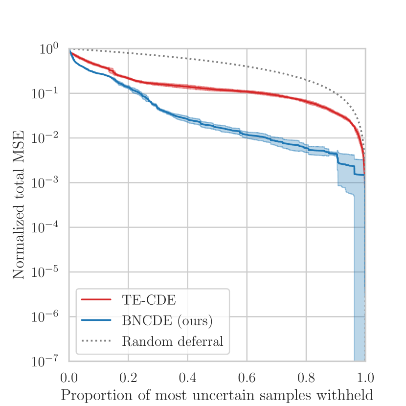
(a) $\Delta=1$

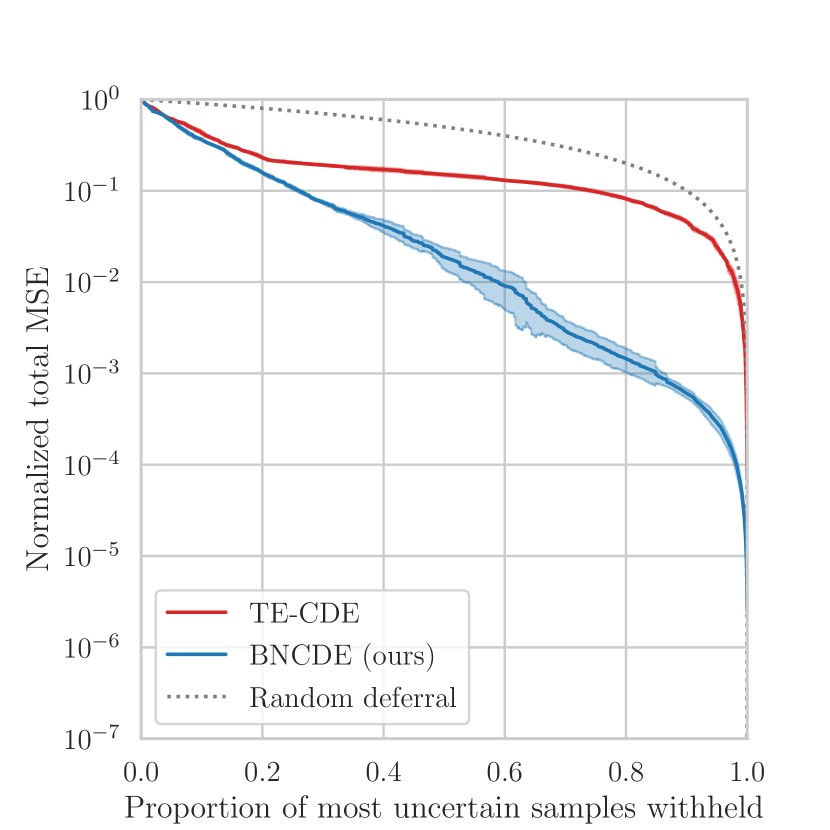
(b) $\Delta=2$

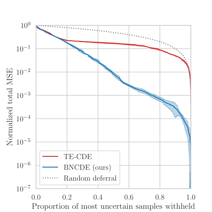
(c) $\Delta=3$

Figure 5: To compare model uncertainty, the normalized MSE of estimated treatment effects between the treatment arms versus deferral rate is shown.

Fig. 5 shows the normalized MSE across different proportions of withheld samples. For TE-CDE with MC dropout, the MSE decreases almost randomly, implying that the MC estimates as a measure of model uncertainty are highly uninformative (and close to random deferral). For our BNCDE, a larger MSE in the treatment effect estimates corresponds to a higher model uncertainty, thus implying that the model uncertainty in our method is more informative.

Extension: We repeat our experiments for informative sampling (see Supplement H). For this, we extend both our BNCDE and TE-CDE using the inverse intensity weighting method from Vanderschueren et al. (2023). We find that our method remains clearly superior.

Conclusion: Our results show the following: (1) Our BNCDE produces posterior predictive CrIs that are faithful. In contrast, the CrIs from TE-CDE can be overconfident, which, in medicine, may lead to treatment decisions that are dangerous. (2) Our BNCDE further provides approximations of the CrIs that are sharper. (3) Our BNCDE generates more informative estimates of model uncertainty compared to TE-CDE with MC dropout. (4) Our BNCDE is further fairly robust against noise and, also, (5) highly effective for longer prediction windows.

Appendix A TE-CDE

In this section, we give a brief overview of the so-called treatment effect neural controlled differential equation (TE-CDE) (Seedat et al., 2022). We present the main ideas of the original TE-CDE model but refer to the original paper for more details. We build upon our notation from Section 3.1.

TE-CDE uses neural controlled differential equations to predict counterfactual outcomes in continuous time. For this, TE-CDE assumes that a hidden state variable $Z_{t}\in\mathbb{R}^{d_{z}}$ is driven by the outcome history, covariate history, and treatment history. The control path is interpolated in continuous time from observational, irregularly sampled data. The hidden state variable $Z_{t}$ encodes information about the potential outcomes for a given treatment assignment. In (Seedat et al., 2022), TE-CDE is trained with an adversarial loss term to enforce balanced representations (see Supplement I for a discussion on balanced representations). However, balanced representations are not the focus of our paper, and we thus omit them for better comparability.

As is common for neural CDEs, TE-CDE encodes the initial outcome variable $Y_{0}$, covariates $X_{0}$ and treatment $A_{0}$ into the hidden state $Z_{0}$ through an embedding network $\eta_{\phi}^{e}:\mathbb{R}^{1+d_{x}+d_{a}}\to\mathbb{R}^{d_{z}}$. The hidden state then serves as the initial condition of the controlled differential equation given by

$$Z_{t}=\int_{0}^{t}f_{\phi}^{e}(Z_{s})\mathop{}\!\mathrm{d}[Y_{s},X_{s},A_{s}],\quad t\in(0,\bar{T}]\quad\text{and}\quad Z_{0}=\eta_{\phi}^{e}(Y_{0},X_{0},A_{0}).$$ (14)

Eq. 14 is the encoder network of TE-CDE. The last hidden state $Z_{\bar{T}}$ is then passed through a decoder to predict the potential outcome $Y_{\bar{T}+\Delta}[a_{(\bar{T},\bar{T}+\Delta]}^{\prime}]$ for an arbitrary but fixed time window $\Delta$ in the future. The decoder is given by the neural CDE

$$Y_{\bar{T}+\Delta}[a_{(\bar{T},\bar{T}+\Delta]}^{\prime}]\approx\eta^{1}_{\phi}(\tilde{Z}_{\Delta}),\quad\tilde{Z}_{\tau}=\int_{0}^{\tau}f_{\phi}^{d}(\tilde{Z}_{s})\mathop{}\!\mathrm{d}a_{\tau}^{\prime},\quad\tau\in(0,\Delta]\quad\text{and}\quad\tilde{Z}_{0}=Z_{\bar{T}},$$ (15)

where $\eta^{d}_{\phi}$ is the read-out mapping. In particular, for a new patient $*$, TE-CDE seeks to approximate the expected value of the potential outcome, given the patient trajectory ${H}_{\bar{t}^{*}}^{*}$. That is, TE-CDE approximates the quantity

$$\mathbb{E}[Y_{\bar{t}^{*}+\Delta}[a_{(\bar{t}^{*},\bar{t}^{*}+\Delta]}^{\prime}]\mid H_{\bar{t}^{*}}^{*}].$$ (16)

Reassuringly, we highlight the following key differences between TE-CDE and our BNCDE:

1. TE-CDE targets Eq. 16 and thus makes a point estimate of the potential outcome at time $\bar{t}^{*}+\Delta$. In contrast, our BNCDE estimates the full posterior predictive distribution of the potential outcome.

2. TE-CDE directly optimizes the neural vector fields $f_{\phi}^{e}$ and $f_{\phi}^{d}$ of the CDE. Instead, our BNCDE parameterizes the distribution of the neural CDE weights with a latent neural SDE. This neural SDE is optimized to shape the posterior distribution of the neural CDE weights given the training data. As such, the architectures of TE-CDE and our BNCDE are vastly different.

3. TE-CDE may employ MC dropout to approximate model uncertainty. However, as we show in our paper, the tailored neural SDEs provide more faithful model uncertainty quantification.

4. TE-CDE does not provide an estimate of the outcome uncertainty quantification. On the other hand, our BNCDE incorporates outcome uncertainty through the likelihood variance $\Sigma_{\bar{t}^{*}+\Delta}$.

5. The training objective of TE-CDE is against the mean squared error (MSE). In contrast, our method optimizes the evidence lower bound (ELBO). The ELBO seeks to balance the expected likelihood under the posterior distribution with the Kullback-Leibler divergence between prior and posterior SDEs. Therefore, our loss naturally incorporates weight regularization.

Appendix B Neural Differential Equations

We provide a brief overview of (1) neural ODEs, (2) neural CDEs, and (3) neural SDEs.

Neural ODEs: Neural ordinary differential equations (ODEs) (Haber & Ruthotto, 2018; Lu et al., 2018) combine neural networks with ordinary differential equations. Recall that, in a traditional residual neural network with $t=1,\ldots,T$ residual layers, the hidden states are defined as

$$Z_{t}=Z_{t-1}+f_{\phi_{t}}(Z_{t-1}),$$ (17)

where $f_{\phi_{t}}(\cdot)$ is the $t$-th residual layer with trainable parameters $\phi_{t}$ and $Z_{0}=X$ is the input data. These update rules correspond to an Euler discretization of a continuous transformation. That is, stacking infinitely many infinitesimal small residual transformations, $f_{\phi}(\cdot)$ defines a vector field induced by the initial value problem

$$Z_{t}=\int_{0}^{t}f_{\phi}(Z_{s},s)\mathop{}\!\mathrm{d}s,\quad Z_{0}=X.$$ (18)

Instead of specifying discrete layers and their parameters, a neural ODE describes the continuous changes of the hidden states over an imaginary time scale. A neural ODE thus learns a continuous flow of transformations: an input $X=Z_{0}$ is passed through an ODE solver to produce an output $\hat{Y}=Z_{T}$. The vector field $f_{\phi}$ is then updated either by propagating the error backward through the solver or using the adjoint method (Chen et al., 2018).

Neural CDEs: Neural controlled differential equations (CDEs) (Kidger et al., 2020) extend the above architecture in order to handle time series data in continuous time. In a neural ODE, all information has to be captured in the input $Z_{0}=X$, i.e., at time $t=0$. Neural CDEs, on the other hand, are able to process time series data. They can thus be seen as the continuous-time analog of recurrent neural networks. For a path of covariate data $X_{t}\in\mathbb{R}^{d_{x}}$, $t\in[0,T]$, a neural CDE is given by an embedding network $\eta_{\phi}^{0}(\cdot)$, a readout mapping $\eta_{\phi}^{1}(\cdot)$, and a neural vector field $f_{\phi}$ that satisfy

$$\hat{Y}=\eta_{\phi}^{1}(Z_{\bar{T}}),\quad Z_{t}=\int_{0}^{t}f_{\phi}(Z_{s},s)\mathop{}\!\mathrm{d}X_{s},\quad t\in(0,\bar{T}]\quad\text{and}\quad Z(0)=\eta_{\phi}^{0}(X_{0}),$$ (19)

where $Z_{t}\in\mathbb{R}^{d_{z}}$ and $f_{\phi}(Z_{t},t)\in\mathbb{R}^{d_{z}\times d_{x}}$. The integral is a Riemann-Stieltjes integral, where $f_{\phi}(Z_{s},s)\mathop{}\!\mathrm{d}X_{s}$ refers to matrix-vector multiplication. Here, the neural differential equation is said to be controlled by $X_{t}$. Under mild regularity conditions, it can be computed as

$$Z_{t}=\int_{0}^{t}f_{\phi}(Z_{s},s)\frac{\mathop{}\!\mathrm{d}X_{s}}{\mathop{}\!\mathrm{d}s}\mathop{}\!\mathrm{d}s,\quad t\in(0,\bar{T}].$$ (20)

Computing the derivative with respect to time requires a representation of the data stream $X_{t}$ for any $t\in[0,\bar{T}]$. Hence, irregularly sampled observations $((t_{0},x_{0}),(t_{1},x_{1}),\ldots,(t_{n},x_{n})=(\bar{t},x_{n}))$ need to be interpolated over time, yielding a continuous time representation $X_{t}$. The neural vector field $f_{\phi}$, the embedding network $\eta_{\phi}^{0}$, and the readout network $\eta_{\phi}^{1}$ are then optimized analogous to the neural ODE. For data interpolation, Morrill et al. (2021) suggest different interpolation schemes for different tasks such as rectilinear interpolation for online prediction.

Neural SDEs: Neural stochastic differential equations (SDEs) (Li et al., 2020) learn stochastic differential equations from data. A neural SDE is given by a drift network $g_{\phi}$ and a diffusion network $\sigma_{\phi}$ that satisfy

$$\omega_{t}=\int_{0}^{t}g_{\phi}(\omega_{s},s)\mathop{}\!\mathrm{d}s+\int_{0}^{t}\sigma_{\phi}(\omega_{s},s)\mathop{}\!\mathrm{d}B_{s},\quad t>0\quad\text{and}\quad\omega_{0}=\xi_{\phi},$$ (21)

where $B_{t}$ is a standard Brownian motion and $\xi_{\phi}\sim\mathcal{N}(\nu_{\phi},\sigma_{\phi})$ is the initial condition.

For two SDEs with shared diffusion coefficient, their Kullback-Leibler (KL) divergence can be computed on path space. This makes neural SDEs particularly suited for variational Bayesian inference. Let $g_{\phi}^{q}$ and $h$ be the drifts of the variational neural SDE and the prior SDE respectively. Let furthermore $\sigma(\omega_{t},t)$ be their shared diffusion coefficient. Tzen & Raginsky (2019); Li et al. (2020) show that the KL-divergence on path space then satisfies

$$D_{\mathrm{KL}}[q_{\phi}^{q}(\omega_{[0,t]})\;\|\;p(\omega_{[0,t]})]=\mathbb{E}_{q_{\phi}^{q}(\omega_{[0,t]})}\left[\int_{0}^{t}\left(({g_{\phi}^{q}(\omega_{s})-h(\omega_{s})})/{\sigma(\omega_{s},s)}\right)^{2}\mathop{}\!\mathrm{d}s\right].$$ (22)

Of note, even for a constant shared diffusion parameter $\sigma(\omega_{t},t)=\sigma$, a variational posterior distribution parameterized this way can approximate the true posterior arbitrarily closely using a sufficiently expressive family of drift functions $g_{\phi}^{q}$ (Tzen & Raginsky, 2019; Xu et al., 2022).

Appendix C Cancer Simulation

The tumor data was simulated according to the lung cancer model by Geng et al. (2017), which has previously been used in (Lim et al., 2018; Bica et al., 2020; Li et al., 2021; Melnychuk et al., 2022; Seedat et al., 2022; Vanderschueren et al., 2023). For more details, we refer to these papers. In particular, we adopt the simulation variant by Vanderschueren et al. (2023), which includes irregularly sampled observations and avoids introducing confounding bias in the treatment assignment mechanism.

The tumor volume, which we referred to as the outcome variable in the main paper, evolves according to an ordinary differential equation:

$${\mathop{}\!\mathrm{d}Y_{t}}=\left[1+\underbrace{\rho\log\left(\frac{K}{Y_{t}}\right)}_{\text{Tumor growth}}-\underbrace{\alpha_{c}c_{t}}_{\text{Chemotherapy}}-\underbrace{(\alpha_{r}d_{t}+\beta_{r}d_{t}^{2})}_{\text{Radiotherapy}}+\underbrace{\epsilon_{t}}_{\text{Noise}}\right]Y_{t}\mathop{}\!\mathrm{d}t,$$ (23)

where $\rho$ is a growth parameter, $K$ is the carrying capacity, $\alpha_{c}$, $\alpha_{r}$ and $\beta_{r}$ control the chemo and radio cell kill, respectively, and $\epsilon_{t}$ introduces randomness into the growth dynamics. The parameters were sampled according to Geng et al. (2017) and are summarized in Table 2. The variables $c_{t}$ and $d_{t}$ are set following the work by Lim et al. (2018); Bica et al. (2020); Seedat et al. (2022). The time $t$ is measured in days.

	Variable	Parameter	Distribution	Value $(\mu,\sigma^{2})$
Tumor growth	Growth parameter	$\rho$	Normal	$(7.00\times 10^{-5},7.23\times 10^{-3})$
	Carrying capacity	$K$	Constant	30
Radiotherapy	Radio cell kill	$\alpha_{r}$	Normal	$(0.0398,0.168)$
	Radio cell kill	$\beta_{r}$	–	Set to $\beta_{r}=10\times\alpha_{r}$
Chemotherapy	Chemo cell kill	$\alpha_{c}$	Normal	$(0.028,7.00\times 10^{-4})$
Noise	–	$\epsilon_{t}$	Normal	$(0,0.01^{2})$

Table 2: Sampling details of parameters used in the tumor simulation model.

We make the following, additional adjustments as informed by prior literature:

• As in (Lim et al., 2018; Bica et al., 2020; Seedat et al., 2022; Vanderschueren et al., 2023), heterogeneity between patients is introduced by modeling different subgroups. Each subgroup differs in their average response to treatment, expressed by the mean values of the normal distributions. For subgroup 1, we increase $\mu(\alpha_{r})$ by $10\%$, and, for subgroup 2, we increase $\mu(\alpha_{c})$ by $10\%$.

• Following Kidger et al. (2020), we add a multivariate counting variable that counts how often each treatment has been administered up to a specific time.

• As in (Vanderschueren et al., 2023), the observation process is governed by an intensity process with history-dependent intensity

  $$\zeta_{t}^{i}=\text{sigmoid}\left[\gamma\left(\frac{\bar{D}^{i}_{t}}{D}-\frac{1}{2}\right)\right],$$ (24)

  where $\gamma$ controls the sampling informativeness, $D=13\,\text{cm}$, and $\bar{D}^{i}_{t}$ is the average tumor diameter over the last 15 days. For our informative sampling experiments in Section 5 and for the additional prediction windows in Supplement G, we set $\gamma=1$. For our experiments in Supplement H, we increased the sampling informativeness to $\gamma=2$.

Treatments are assigned according to either a concurrent or a sequential treatment arm (Curran et al., 2011). That is, patients receive treatment either (i) weekly chemotherapy for five weeks and then radiotherapy for another five weeks or (ii) biweekly chemotherapy and radiotherapy for ten weeks. Patients are randomly divided between the two treatment regimes. For any patient in the test data, we simulate both the factual outcome under the assigned treatment arm, and the counterfactual outcome under the unassigned treatment arm.

For each training, validation and testing, our observed time window is 55 days with an additional prediction window of up to 5 days. For training and validation, we simulated 10000 and 1000 observations, respectively. For testing, we simulated the trajectories and the outcomes for 10000 patients under both treatment arms, respectively. We standardized our data with the training set.

Appendix D Variational Approximations

We provide a detailed derivation of (1) our approximate posterior predictive distribution and (2) our evidence lower bound.

Notation: We slightly abuse notation for better readability. We denote the expectation with respect to the stochastic process $\omega_{t}$ on path space as

$$\int(\cdot)\mathop{}\!\mathrm{d}p(\omega_{[0,\bar{T}]})=\mathbb{E}_{p(\omega_{[0,\bar{T}]})}[(\cdot)].$$ (25)

The analogue applies for $\tilde{\omega}_{\tau}$.

Approximate posterior predictive distribution: In the Bayesian framework, the posterior predictive distribution of the outcome of interest $Y_{\bar{t}^{*}+\Delta}[a_{(\bar{t}^{*},\bar{t}^{*}+\Delta]}^{\prime}]$ given observed inputs $h_{\bar{t}^{*}}^{*}$ and training data $\mathcal{H}$ is the expectation of the outcome likelihood under the weight posterior distribution. Hence, we approximate the posterior predictive distribution via

$$p(Y_{\bar{t}^{*}+\Delta}[a_{(\bar{t}^{*},\bar{t}^{*}+\Delta]}^{\prime}]\mid h_{\bar{t}^{*}}^{*},\mathcal{H})$$ (26)

$$= \int p(Y_{\bar{t}^{*}+\Delta}[a_{(\bar{t}^{*},\bar{t}^{*}+\Delta]}^{\prime}]\mid h_{\bar{t}^{*}}^{*},\tilde{\omega}_{[0,\Delta]},\omega_{[0,\bar{t}^{*}]})\mathop{}\!\mathrm{d}p(\tilde{\omega}_{[0,\Delta]},\omega_{[0,\bar{t}^{*}]}\mid\mathcal{H})$$ (27)

$$= \int p(Y_{\bar{t}^{*}+\Delta}[a_{(\bar{t}^{*},\bar{t}^{*}+\Delta]}^{\prime}]\mid h_{\bar{t}^{*}}^{*},\tilde{\omega}_{[0,\Delta]},\omega_{[0,\bar{t}^{*}]})\mathop{}\!\mathrm{d}p(\tilde{\omega}_{[0,\Delta]}\mid\omega_{[0,\bar{t}^{*}]},\mathcal{H})\mathop{}\!\mathrm{d}p(\omega_{[0,\bar{t}^{*}]}\mid\mathcal{H})$$ (28)

$$\approx \int p(Y_{\bar{t}^{*}+\Delta}[a_{(\bar{t}^{*},\bar{t}^{*}+\Delta]}^{\prime}]\mid h_{\bar{t}^{*}}^{*},\tilde{\omega}_{[0,\Delta]},\omega_{[0,\bar{t}^{*}]})\mathop{}\!\mathrm{d}q_{\phi}^{d}(\tilde{\omega}_{[0,\Delta]})\mathop{}\!\mathrm{d}q_{\phi}^{e}(\omega_{[0,\bar{t}^{*}]})$$ (29)

$$= \mathbb{E}_{q_{\phi}^{e}(\omega_{[0,\bar{t}^{*}]})}\left[\mathbb{E}_{q_{\phi}^{d}(\tilde{\omega}_{[0,\Delta]})}\left[p(Y_{\bar{t}^{*}+\Delta}[a_{(\bar{t}^{*},\bar{t}^{*}+\Delta]}^{\prime}]\mid\tilde{\omega}_{[0,\Delta]},\omega_{[0,\bar{t}^{*}]},h_{\bar{t}^{*}}^{*})\right]\right].$$ (30)

Evidence lower bound: Recall that, in our notation, a training sample is ${h_{\bar{t}^{i}+\Delta}^{i}=h_{(\bar{t}^{i}+\Delta)^{-}}^{i}\cup\{y_{\bar{t}^{i}+\Delta}^{i}\}}$, where $h_{(\bar{t}^{i}+\Delta)^{-}}^{i}$ is the training input and $y_{\bar{t}^{i}+\Delta}^{i}$ the target. Our objective is an ELBO maximization, which we derive via

$$\log p(y_{\bar{t}^{i}+\Delta}^{i}\mid h_{(\bar{t}^{i}+\Delta)^{-}}^{i})$$ (31)

$$= \log\int p(y_{\bar{t}^{i}+\Delta}^{i}\mid h_{(\bar{t}^{i}+\Delta)^{-}}^{i},\tilde{\omega}_{[0,\Delta]},\omega_{[0,\bar{t}^{i}]})\mathop{}\!\mathrm{d}p(\tilde{\omega}_{[0,\Delta]},\omega_{[0,\bar{t}^{i}]})$$ (32)

$$= \log\int p(y_{\bar{t}^{i}+\Delta}^{i}\mid h_{(\bar{t}^{i}+\Delta)^{-}}^{i},\tilde{\omega}_{[0,\Delta]},\omega_{[0,\bar{t}^{i}]})\mathop{}\!\mathrm{d}p(\tilde{\omega}_{[0,\Delta]})\mathop{}\!\mathrm{d}p(\omega_{[0,\bar{t}^{i}]})$$ (33)

$$= \log\int p(y_{\bar{t}^{i}+\Delta}^{i}\mid h_{(\bar{t}^{i}+\Delta)^{-}}^{i},\tilde{\omega}_{[0,\Delta]},\omega_{[0,\bar{t}^{i}]})\left(\frac{q_{\phi}^{d}(\tilde{\omega}_{[0,\Delta]})q_{\phi}^{e}(\omega_{[0,\bar{t}^{i}]})}{p(\tilde{\omega}_{[0,\Delta]})p(\omega_{[0,\bar{t}^{i}]})}\right)^{-1}\mathop{}\!\mathrm{d}q_{\phi}^{d}(\tilde{\omega}_{[0,\Delta]})\mathop{}\!\mathrm{d}q_{\phi}^{e}(\omega_{[0,\bar{t}^{i}]})$$ (34)

$$\geq \int\Bigg{[}\log p(y_{\bar{t}^{i}+\Delta}^{i}\mid h_{(\bar{t}^{i}+\Delta)^{-}}^{i},\tilde{\omega}_{[0,\Delta]},\omega_{[0,\bar{t}^{i}]})$$

$$\qquad-\log\left(\frac{q_{\phi}^{d}(\tilde{\omega}_{[0,\Delta]})}{p(\tilde{\omega}_{[0,\Delta]})}\right)-\log\left(\frac{q_{\phi}^{e}(\omega_{[0,\bar{t}^{i}]})}{p(\omega_{[0,\bar{t}^{i}]})}\right)\Bigg{]}\mathop{}\!\mathrm{d}q_{\phi}^{d}(\tilde{\omega}_{[0,\Delta]})\mathop{}\!\mathrm{d}q_{\phi}^{e}(\omega_{[0,\bar{t}^{i}]})$$ (35)

$$= \mathbb{E}_{q_{\phi}^{e}(\omega_{[0,\bar{t}^{i}]})}\Big{\{}\mathbb{E}_{q_{\phi}^{d}(\tilde{\omega}_{[0,\Delta]})}\Big{[}\log p(y_{\bar{t}^{i}+\Delta}^{i}\mid\tilde{\omega}_{[0,\Delta]},\omega_{[0,\bar{t}^{i}]},h_{(\bar{t}^{i}+\Delta)^{-}}^{i})\Big{]}\Big{\}}$$

$$\qquad-D_{\mathrm{KL}}[q_{\phi}^{d}(\tilde{\omega}_{[0,\Delta]})\;\|\;p(\tilde{\omega}_{[0,\Delta]})]-D_{\mathrm{KL}}[q_{\phi}^{e}(\omega_{[0,\bar{t}^{i}]})\;\|\;p(\omega_{[0,\bar{t}^{i}]})],$$ (36)

where Eq. 32 follows from the standard pairwise independence assumption of inputs and weights, Eq. 33 is due to the independence of the OU priors, and Eq. 35 follows from Jensen’s inequality.

The ELBO objective is maximized for ${q_{\phi}^{d}(\tilde{\omega}_{[0,\Delta]})=p(\tilde{\omega}_{[0,\Delta]}\mid h_{\bar{t}^{i}+\Delta}^{i},\omega_{[0,\bar{t}^{i}]})}$ and ${q_{\phi}^{e}(\omega_{[0,\bar{t}^{i}]})=p(\omega_{[0,\bar{t}^{i}]}\mid h_{\bar{t}^{i}+\Delta}^{i})}$. We can see this by substituting in the true weight posteriors into Eq. 35. This yields

$$\int\Bigg{[}\log p(y_{\bar{t}^{i}+\Delta}^{i}\mid h_{(\bar{t}^{i}+\Delta)^{-}}^{i},\tilde{\omega}_{[0,\Delta]},\omega_{[0,\bar{t}^{i}]})-\log\left(\frac{p(\tilde{\omega}_{[0,\Delta]}\mid h_{\bar{t}^{i}+\Delta}^{i},\omega_{[0,\bar{t}^{i}]})}{p(\tilde{\omega}_{[0,\Delta]})}\right)$$

$$\qquad-\log\left(\frac{p(\omega_{[0,\bar{t}^{i}]}\mid h_{\bar{t}^{i}+\Delta}^{i})}{p(\omega_{[0,\bar{t}^{i}]})}\right)\Bigg{]}\mathop{}\!\mathrm{d}p(\tilde{\omega}_{[0,\Delta]}\mid h_{\bar{t}^{i}+\Delta}^{i},\omega_{[0,\bar{t}^{i}]})\mathop{}\!\mathrm{d}p(\omega_{[0,\bar{t}^{i}]}\mid h_{\bar{t}^{i}+\Delta}^{i})$$ (37)

$$= \int\log\left(\frac{p(y_{\bar{t}^{i}+\Delta}^{i}\mid h_{(\bar{t}^{i}+\Delta)^{-}}^{i},\tilde{\omega}_{[0,\Delta]},\omega_{[0,\bar{t}^{i}]})p(\tilde{\omega}_{[0,\Delta]},\omega_{[0,\bar{t}^{i}]})}{p(\tilde{\omega}_{[0,\Delta]},\omega_{[0,\bar{t}^{i}]}\mid h_{(\bar{t}^{i}+\Delta)^{-}}^{i},y_{\bar{t}^{i}+\Delta}^{i})}\right)\mathop{}\!\mathrm{d}p(\tilde{\omega}_{[0,\Delta]},\omega_{[0,\bar{t}^{i}]}\mid h_{\bar{t}^{i}+\Delta}^{i})$$ (38)

$$= \int\log\left(\frac{p(y_{\bar{t}^{i}+\Delta}^{i},\tilde{\omega}_{[0,\Delta]},\omega_{[0,\bar{t}^{i}]})\mid h_{(\bar{t}^{i}+\Delta)^{-}}^{i})}{p(\tilde{\omega}_{[0,\Delta]},\omega_{[0,\bar{t}^{i}]}\mid h_{(\bar{t}^{i}+\Delta)^{-}}^{i},y_{\bar{t}^{i}+\Delta}^{i})}\right)\mathop{}\!\mathrm{d}p(\tilde{\omega}_{[0,\Delta]},\omega_{[0,\bar{t}^{i}]}\mid h_{\bar{t}^{i}+\Delta}^{i})$$ (39)

$$= \int\log\left(\frac{p(\tilde{\omega}_{[0,\Delta]},\omega_{[0,\bar{t}^{i}]}\mid h_{(\bar{t}^{i}+\Delta)^{-}}^{i},y_{\bar{t}^{i}+\Delta}^{i})p(y_{\bar{t}^{i}+\Delta}^{i}\mid h_{(\bar{t}^{i}+\Delta)^{-}}^{i})}{p(\tilde{\omega}_{[0,\Delta]},\omega_{[0,\bar{t}^{i}]}\mid h_{(\bar{t}^{i}+\Delta)^{-}}^{i},y_{\bar{t}^{i}+\Delta}^{i})}\right)\mathop{}\!\mathrm{d}p(\tilde{\omega}_{[0,\Delta]},\omega_{[0,\bar{t}^{i}]}\mid h_{\bar{t}^{i}+\Delta}^{i})$$ (40)

$$= \int\log p(y_{\bar{t}^{i}+\Delta}^{i}\mid h_{(\bar{t}^{i}+\Delta)^{-}}^{i})\mathop{}\!\mathrm{d}p(\tilde{\omega}_{[0,\Delta]},\omega_{[0,\bar{t}^{i}]}\mid h_{\bar{t}^{i}+\Delta}^{i})$$ (41)

$$= \log p(y_{\bar{t}^{i}+\Delta}^{i}\mid h_{(\bar{t}^{i}+\Delta)^{-}}^{i}),$$ (42)

where Eq. 39 follows again from prior independence of input data and weights and the fact that $h_{\bar{t}^{i}+\Delta}^{i}=h_{(\bar{t}^{i}+\Delta)^{-}}^{i}\cup\{y_{\bar{t}^{i}+\Delta}^{i}\}$.

Appendix E Numerical Computation of the Evidence Lower Bound

The objective of our BNCDE is the evidence lower bound (ELBO), which is approximated after the forward pass of the numerical SDE solver.

Recall that, for an observation $i$, the ELBO is given by

$$\log p(y_{\bar{t}^{i}+\Delta}^{i}\mid h_{(\bar{t}^{i}+\Delta)^{-}}^{i})\geq\mathbb{E}_{q_{\phi}^{e}(\omega_{[0,\bar{t}^{i}]})}\Big{\{}\mathbb{E}_{q_{\phi}^{d}(\tilde{\omega}_{[0,\Delta]})}\Big{[}\log p(y_{\bar{t}^{i}+\Delta}^{i}\mid\tilde{\omega}_{[0,\Delta]},\omega_{[0,\bar{t}^{i}]},h_{(\bar{t}^{i}+\Delta)^{-}}^{i})\Big{]}\Big{\}}\\ -D_{\mathrm{KL}}[q_{\phi}^{d}(\tilde{\omega}_{[0,\Delta]})\;\|\;p(\tilde{\omega}_{[0,\Delta]})]-D_{\mathrm{KL}}[q_{\phi}^{e}(\omega_{[0,\bar{t}^{i}]})\;\|\;p(\omega_{[0,\bar{t}^{i}]})].$$ (43)

We approximate the expectations with respect to $q_{\phi}^{e}(\omega_{[0,\bar{t}^{i}]})$ and $q_{\phi}^{d}(\omega_{[0,\Delta]})$ with Monte Carlo samples $\omega_{\underline{[0,\bar{t}^{i}]}}^{j}$ and $\tilde{\omega}_{\underline{[0,\Delta]}}^{k}$ of the weight trajectories from the numerical SDE solver. That is, we compute the expected likelihood via

$$\mathbb{E}_{q_{\phi}^{e}(\omega_{[0,\bar{t}^{i}]})}\Big{\{}\mathbb{E}_{q_{\phi}^{d}(\tilde{\omega}_{[0,\Delta]})}\Big{[}\log p(y_{\bar{t}^{i}+\Delta}^{i}\mid\tilde{\omega}_{[0,\Delta]},\omega_{[0,\bar{t}^{i}]},h_{(\bar{t}^{i}+\Delta)^{-}}^{i})\Big{]}\Big{\}}$$ (44)

$$\approx \frac{1}{J}\sum_{\omega_{\underline{[0,\bar{t}^{i}]}}^{j}\sim q_{\phi}^{e}}\Big{\{}\frac{1}{K}\sum_{\tilde{\omega}_{\underline{[0,\Delta]}}^{k}\sim q_{\phi}^{d}}\Big{[}\log p(y_{\bar{t}^{i}+\Delta}^{i}\mid\tilde{\omega}_{\underline{[0,\Delta]}}^{k},\omega_{\underline{[0,\bar{t}^{i}]}}^{j},h_{(\bar{t}^{i}+\Delta)^{-}}^{i})\Big{]}\Big{\}},$$ (45)

where $\underline{[0,\bar{t}^{i}]}$ and $\underline{[0,\Delta]}$ are grid approximations of $[0,\bar{t}^{i}]$ and $[0,\Delta]$, respectively.

The Kullback-Leibler (KL) divergences between priors and variational posteriors on path space can also be computed through Monte Carlo approximations. Here, we focus on the KL-divergence in the encoder component; the decoder part follows analogously. Recall that we seek to compute the KL-divergence between the solutions of the SDEs

$$\mathop{}\!\mathrm{d}\omega_{t}=\begin{cases}g_{\phi}^{e}(\omega_{t})\mathop{}\!\mathrm{d}t+\sigma\mathop{}\!\mathrm{d}B_{t}\\ h^{e}(\omega_{t})\mathop{}\!\mathrm{d}t+\sigma\mathop{}\!\mathrm{d}B_{t}.\end{cases}$$ (46)

Previously, Tzen & Raginsky (2019) and Li et al. (2020) have shown that for two stochastic differential equations with shared diffusion coefficient $\sigma$, the KL-divergence on path space satisfies

$$D_{\mathrm{KL}}[q_{\phi}^{e}(\omega_{[0,\bar{t}^{i}]})\;\|\;p(\omega_{[0,\bar{t}^{i}]})]=\mathbb{E}_{q_{\phi}^{e}(\omega_{[0,\bar{t}^{i}]})}\left[\int_{0}^{\bar{t}^{i}}\left(({g_{\phi}^{e}(\omega_{t})-h^{e}(\omega_{t})})/{\sigma}\right)^{2}\mathop{}\!\mathrm{d}t\right].$$ (47)

Therefore, it can be approximated with Monte Carlo samples from the numerical SDE solver. That is, we compute

$$\mathbb{E}_{q_{\phi}^{e}(\omega_{[0,\bar{t}^{i}]})}\left[\int_{0}^{\bar{t}^{i}}\left(({g_{\phi}^{e}(\omega_{t})-h^{e}(\omega_{t})})/{\sigma}\right)^{2}\mathop{}\!\mathrm{d}t\right]\approx\frac{1}{J}\sum_{\omega_{\underline{[0,\bar{t}^{i}]}}^{j}\sim q_{\phi}^{e}}\left[\int_{\underline{[0,\bar{t}^{i}]}}\left(({g_{\phi}^{e}(\omega_{t}^{j})-h^{e}(\omega_{t}^{j})})/{\sigma}\right)^{2}\mathop{}\!\mathrm{d}t\right],$$ (48)

where $\int_{\underline{[0,\bar{t}^{i}]}}(\cdot)\mathop{}\!\mathrm{d}t$ denotes the integral approximation from the SDE solver. In other words, for each Monte Carlo particle $j$, we pass the KL-divergence term as additional state through the SDE solver and then take the Monte Carlo average at time $\bar{t}^{i}$.

Appendix F Implementation Details

In the following, we summarize the implementation details of our BNCDE and TE-CDE. Experiments were carried out on $1\times$ NVIDIA A100-PCIE-40GB. Training of BNCDE and TE-CDE took approximately 34 hours and 22 hours, respectively.

The hyperparameters of TE-CDE were taken from the original work (Seedat et al., 2022). For both training and testing, the dropout probabilities in the prediction head were set to $p=0.1$. As in our BNCDE, we included the time covariate $t$ as an input to TE-CDE, as this improved performance.

We optimized the hidden layers of the neural SDEs drift over $\{16,$ ${(16,16)},$ ${(16,64,16)},$ ${(16,64,64,16)},$ ${(16,64,64,64,16)}\}$ and the diffusion coefficient $\sigma$ over $\{0.01,0.001,0.0001\}$. We used the same neural SDE configuration for both the encoder and the decoder. Our performance metric was the ELBO objective on the validation set. We only optimized the hyperparameters for the prediction window $\Delta=1$ and then used the same configurations for $\Delta=2,\ldots,5$. For better comparability, our BNCDE had the same hyperparameter specifications as TE-CDE where possible.

For both our BNCDE and TE-CDE, we increased the learning rates of the linear embedding and prediction networks compared to the original TE-CDE implementation for more efficient training (Kidger et al., 2020). Further, we used cubic Hermite splines with backward differences in the neural CDEs, which have been shown to be superior to linear interpolation (Morrill et al., 2021). As we want to understand the true source of performance gain, we removed the balancing loss term in TE-CDE as there is no confounding in our data. However, we emphasize that the balancing loss term could easily be added to our BNCDE, as we show in our extended analysis in Supplement I).

Table 3 lists the selected hyperparameters.

Component	Hyperparameter	BNCDE (ours)	TE-CDE (Seedat et al., 2022)
General	Batch size	64	64
	Optimizer	Adam	Adam
	Max. number of epochs	$500$	$500$
	Patience	$10$	$10$
	MC samples training	10	10
	MC samples prediction	100	100
	Hidden state size $d_{z}$	8	8
	Interpolation method	Cubic Hermite splines	Cubic Hermite splines
Differential equation solver	Solver	Euler-Maruyama	Euler
	Step size	Adaptive	Adaptive
Embedding network	Learning rate	$10^{-3}$	$10^{-3}$
	Hidden layers	—	—
	Output activation	—	—
Neural CDEs	Learning rate	—	$10^{-4}$
	Hidden layers	$2$	$2$
	Hidden dimensions	$(128,128)$	$(128,128)$
	Hidden activations	ReLU	ReLU
	Output activation	tanh	tanh
Neural SDEs	Learning rate	$10^{-4}$	—
	Hidden layers	$5$	—
	Hidden dimensions	$(16,64,64,64,16)$	—
	Hidden activations	ReLU	—
	Output activation	—	—
	Diffusion coefficient	0.001	—
Prediction network	Learning rate	$10^{-3}$	$10^{-3}$
	Hidden layers	—	—
	Output activation	( — , softplus)	—
	Dropout probability	—	0.1
Intensity network (only for Supplement H)	Learning rate	$10^{-3}$	$10^{-3}$
	Hidden layers	—	—
	Output activation	sigmoid	sigmoid

Table 3: Hyperparameters of BNCDE and TE-CDE. Hyperparameters of TE-CDE were taken from (Seedat et al., 2022). Our BNCDE used the same hyperparameters where possible.

Appendix G Additional Prediction Windows

We repeat the experiments from Section 5 for the prediction windows $\Delta=4$ and $\Delta=5$. We report the results in Figures 6 and 7, respectively. The results are consistent with our main paper: (i) The credible intervals generated by our BNCDE remain faithful and sharp. In contrast, TE-CDE produces unfaithful CrIs. (ii) The point estimates of the outcome by our BNCDE are more stable under increasing noise in the data generation. (iii) The model uncertainty of our BNCDE is better calibrated.

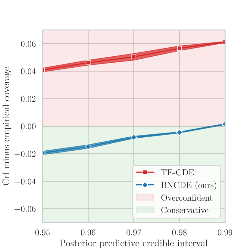
(a) CrI coverage

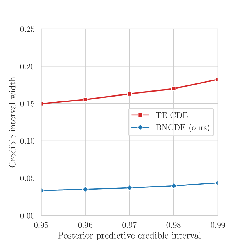
(b) CrI width

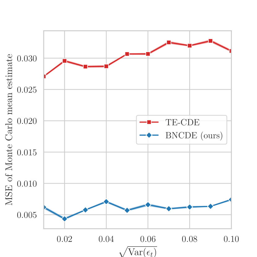
(c) Error in point estimates

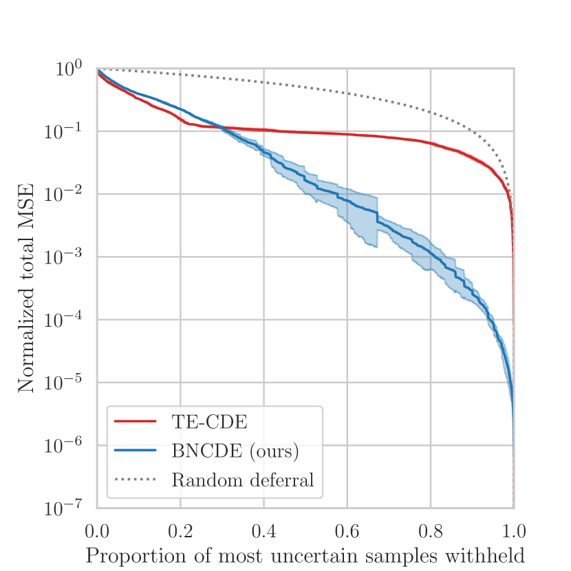
(d) Comparison of model uncertainty

Figure 6: We repeat our experiments from Section 5. Reported are the results for the prediction window $\Delta=4$.

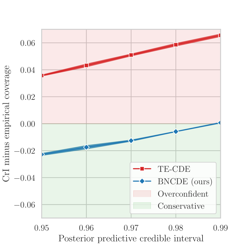
(a) CrI coverage

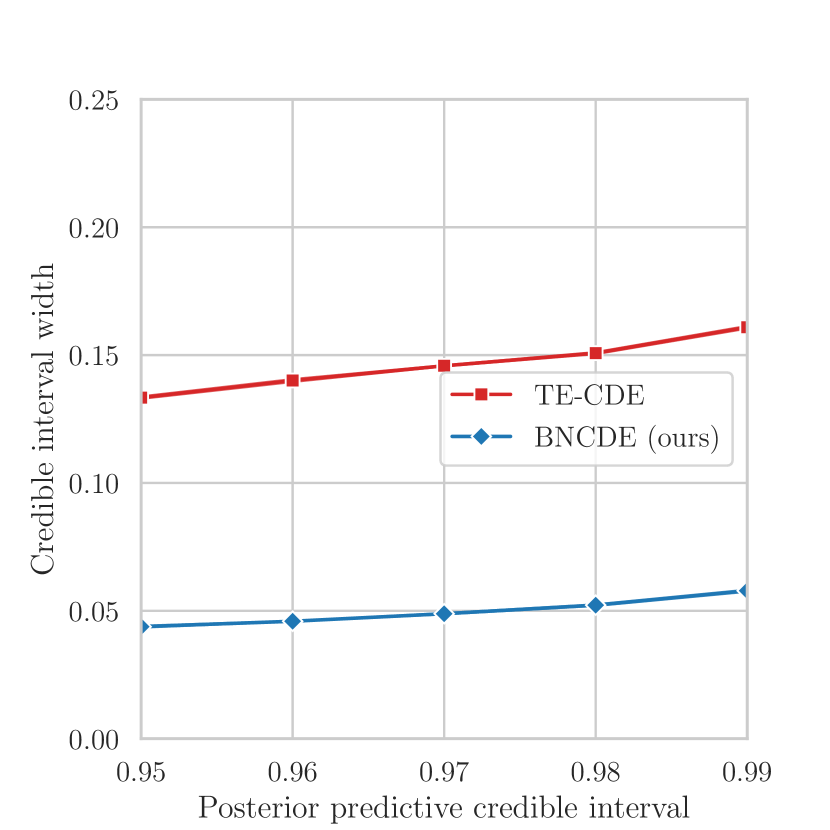
(b) CrI width

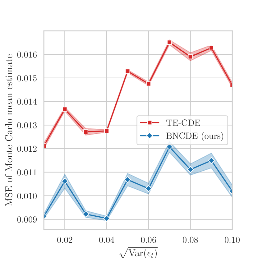
(c) Error in point estimates

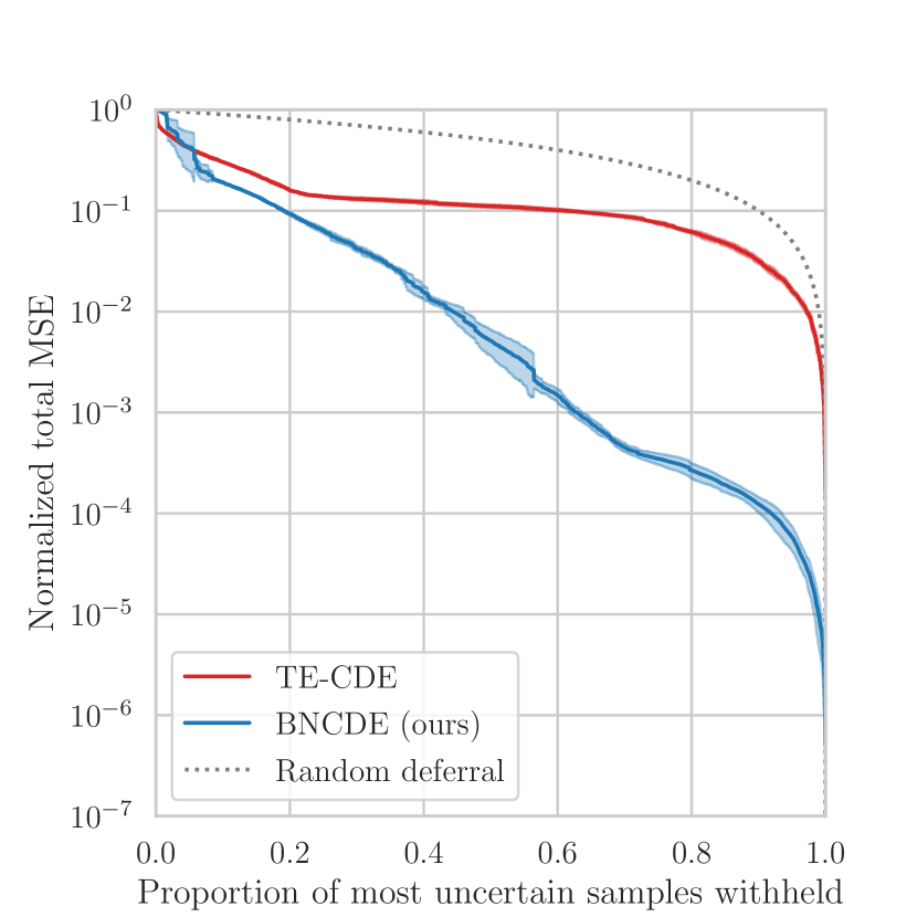
(d) Comparison of model uncertainty

Figure 7: We repeat our experiments from Section 5. Reported are the results for the prediction window $\Delta=5$.

Appendix H Extension to Informative Sampling

We show that our BNCDE is superior over TE-CDE, even when used together with the informative sampling framework from Vanderschueren et al. (2023). The motivation for this is that the observation times of an outcome may themselves contain valuable information about the health status of a particular patient. For example, patients in a more severe state of health are likely to be visited more often, leading to a correspondingly higher observation intensity. To address such informative sampling, Vanderschueren et al. (2023) propose to weight the training objective with the inverse observation intensity. To achieve this, they introduce an additional prediction head for TE-CDE, which estimates the observation intensities. The inverse estimated observation intensities are then used to weight the training objective, which has been shown to improve performance in outcome estimation. This extension of TE-CDE is called the TESAR-CDE.

Changes to tumor growth simulator: We extend our simulation setup as follows. In the tumor growth simulator (see Supplement C), the observation times are determined by an intensity process with an intensity function

$$\zeta_{t}^{i}=\text{sigmoid}\left[\gamma\left(\frac{\bar{D}^{i}_{t}}{D}-\frac{1}{2}\right)\right],$$ (49)

where $\gamma$ controls the sampling informativeness, $D=13\text{cm}$ and $\bar{D}^{i}_{t}$ is the average tumor diameter over the last 15 days. For higher values of $\gamma$, the total number of observed outcomes reduces but the informativeness of each observation timestamp increases. We later change $\gamma=2.0$ to introduce informative sampling.

Changes to our BNCDE: We can easily incorporate the inverse intensity weighting into our BNCDE to account for informative sampling. The final hidden representation $\tilde{Z}_{\Delta}^{i}$ of patient $i$ is additionally passed through a second prediction head $\eta_{\phi}^{\zeta}$ to estimate the observation intensity via

$$\hat{\zeta}_{\bar{t}^{i}+\Delta}^{i}=\eta_{\phi}^{\zeta}(\tilde{Z}_{\Delta}^{i}).$$ (50)

The evidence lower bound (ELBO) for a patient observation $i$ is then weighted with the inverse estimated observation intensity, i.e.,

$$\text{ELBO}^{i}/\hat{\zeta}_{\bar{t}^{i}+\Delta}^{i}.$$ (51)

Experiments: We repeat the experiments from Section 5, where we increase the level of informativeness $\gamma$ from $1.0$ to $2.0$. We focus on the prediction window $\Delta=1$ with inverse intensity weighting enabled for both methods.

We benchmark our BNCDE with TESAR-CDE. For TESAR-CDE, we enable MC dropout in the outcome prediction head $\eta_{\phi}^{p}$ but not in the intensity prediction head $\eta_{\phi}^{\zeta}$. We provide implementation details of $\eta_{\phi}^{\zeta}$ in Supplement F. For both TESAR-CDE and our extended BNCDE, optimization of $\eta_{\phi}^{\zeta}$ is performed as in the original work by Vanderschueren et al. (2023). That is, the error in the estimated observation intensity is not propagated through the whole computational graph but only through $\eta_{\phi}^{\zeta}$.

Results: Fig 8 shows, that in the informative sampling setting, our method remains superior. Our BNCDE (i) produces more faithful and sharper credible interval approximations; (ii) generates more stable point estimates of the outcome under increasing noise; and (iii) has a better calibrated model uncertainty. In sum, this demonstrates the effectiveness of our BNCDE even for informative sampling.

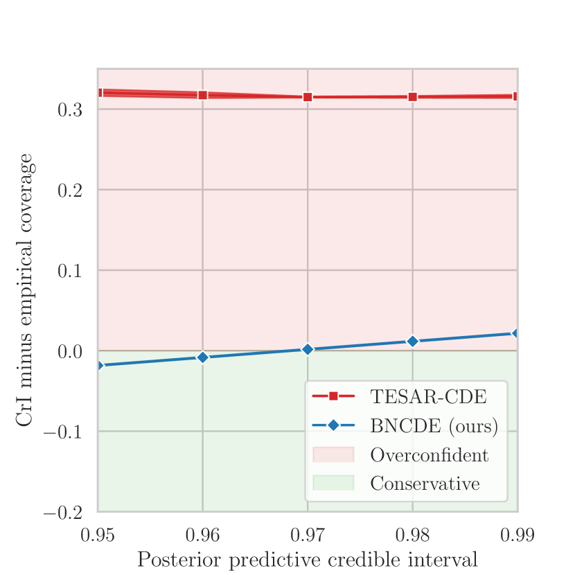
(a) CrI coverage

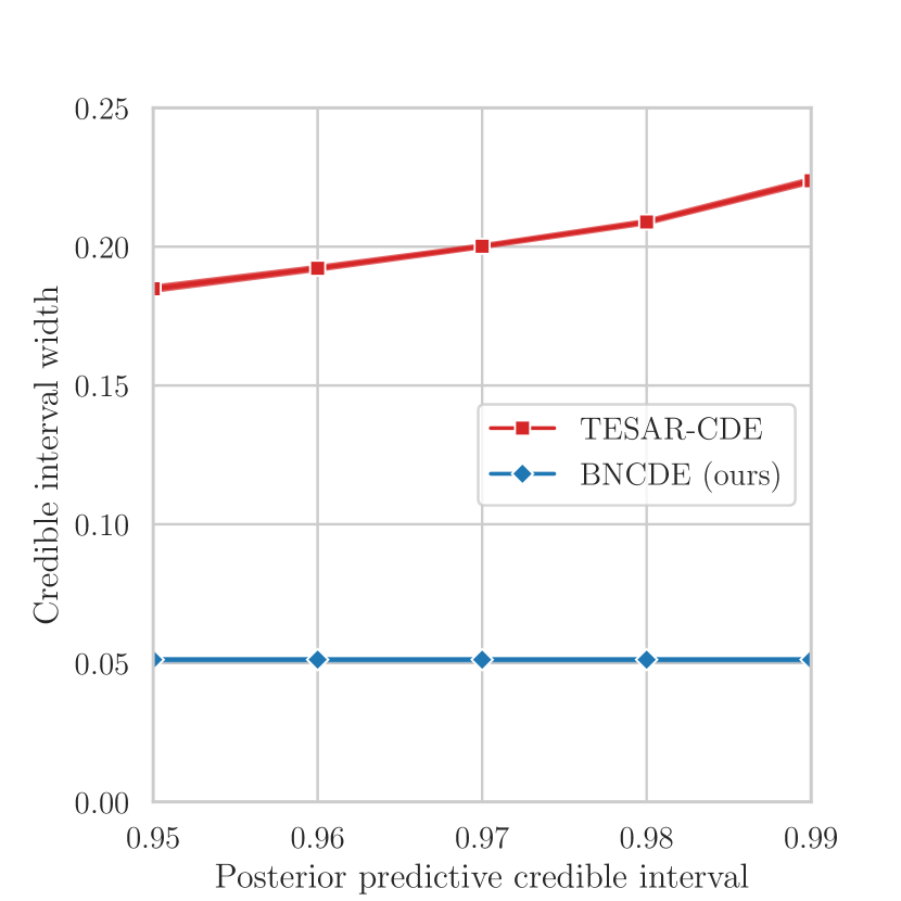
(b) CrI width

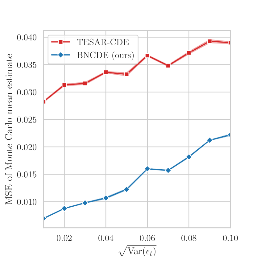
(c) Error in point estimates

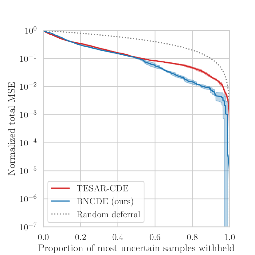
(d) Comparison of model uncertainty

Figure 8: We repeat the experiments for settings with informative sampling. For this, we increase the informativeness parameter in the tumor growth simulator to $\gamma=2.0$. Following (Vanderschueren et al., 2023), we weight the training objective with the estimated inverse observation intensity. We benchmark our extended BNCDE against TESAR-CDE (Vanderschueren et al., 2023), for which we enable MC dropout in the outcome prediction head.

Appendix I Balanced Representations

Some prior works on estimating heterogeneous treatment effects propose to learn balanced representations that are non-predictive of the treatment (Bica et al., 2020; Seedat et al., 2022). The idea is to mimic randomized clinical trials and reduce finite sample estimation error. However, for time-varying treatment effects, this approach has several drawbacks:

1. Learning guarantees only exit in static (i.e., non-time-varying) settings (Shalit et al., 2017). Thus, balanced representations do not help with reducing bias due to identifiability issues induced by time-varying confounders. For this, proper adjustment methods such as G-computation or inverse-propensity weighting would be necessary (Pearl, 2009; Robins & Hernán, 2009).

2. Even in static settings, methods based on balanced representations impose invertibility assumptions on the learned representations (Shalit et al., 2017). This is highly unrealistic in time-varying settings, where representations not only incorporate information about the confounders but also about the full patient history.

3. Because invertibility is difficult to ensure, balanced representations may actually increase bias. We refer to Curth & van der Schaar (2021) and Melnychuk et al. (2023b) for a detailed discussion on this issue. Again, this is particularly detrimental in time-varying settings.

Nevertheless, we emphasize that balanced representations could be easily integrated into our BNCDE. To do this, an adversarial training objective can be added to enforce treatment agnostic hidden representations $Z_{t}$ and $\tilde{Z}_{\tau}$, i.e., representations that are non-informative of the assigned sequence of treatments. To this end, the architecture in Figure 1 can be extended with a second prediction head $\eta_{\phi}^{a}$ as in (Seedat et al., 2022). Here, $\eta_{\phi}^{a}$ predicts the probability of treatment $\hat{p}_{t}^{a}$ at time $t$. For a sequence of treatments with treatment decisions at irregular timestamps $\{t_{1},\ldots,t_{m}\}$, the prediction head is trained to maximize the binary cross-entropy given by

$$\text{BCE}=-\frac{1}{m}\sum_{j=1}^{m}a_{t_{j}}\log(\hat{p}_{t_{j}}^{a})+(1-a_{t_{j}})\log(1-\hat{p}_{t_{j}}^{a}).$$ (52)

The overall objective is then to maximize the weighted sum

$$\text{ELBO}\>+\>\alpha\>\text{BCE},$$ (53)

where $\alpha$ is a balancing hyperparameter.

In summary, balanced representations are a heuristic approach to reduce finite-sample bias, because proper adjustment methods are often not applicable in practice. For example, G-computation requires learning the conditional distribution of time-varying covariates, which is infeasible in high-dimensional settings (Melnychuk et al., 2022). In our paper, we decided not to incorporate balanced representations due to the reasons described above. This is consistent with previous works in the literature (Curth & van der Schaar, 2021; Vanderschueren et al., 2023).

References

- Alaa & van der Schaar (2017) Ahmed M. Alaa and Mihaela van der Schaar. Bayesian inference of individualized treatment effects using multi-task Gaussian processes. In NeurIPS, 2017.
- Allam et al. (2021) Ahmed Allam, Stefan Feuerriegel, Michael Rebhan, and Michael Krauthammer. Analyzing patient trajectories with artificial intelligence. Journal of Medical Internet Research, 23(12):e29812, 2021.
- Bica et al. (2020) Ioana Bica, Ahmed M. Alaa, James Jordon, and Mihaela van der Schaar. Estimating counterfactual treatment outcomes over time through adversarially balanced representations. In ICLR, 2020.
- Bica et al. (2021) Ioana Bica, Ahmed M. Alaa, Craig Lambert, and Mihaela van der Schaar. From real-world patient data to individualized treatment effects using machine learning: Current and future methods to address underlying challenges. Clinical Pharmacology and Therapeutics, 109(1):87–100, 2021.
- Brouwer et al. (2022) Edward De Brouwer, Javier González Hernández, and Stephanie Hyland. Predicting the impact of treatments over time with uncertainty aware neural differential equations. In AISTATS, 2022.
- Chen et al. (2018) Ricky T. Q. Chen, Yulia Rubanova, Jesse Bettencourt, and David Duvenaud. Neural ordinary differential equations. In NeurIPS, 2018.
- Curran et al. (2011) Walter J. Curran, Rebecca Paulus, Corey J. Langer, Ritsuko Komaki, Jin S. Lee, Stephen Hauser, Benjamin Movsas, Todd Wasserman, Seth A. Rosenthal, Elizabeth Gore, Mitchell Machtay, William Sause, and James D. Cox. Sequential vs. concurrent chemoradiation for stage III non-small cell lung cancer: Randomized phase III trial RTOG 9410. Journal of the National Cancer Institute, 103(19):1452–1460, 2011.
- Curth & van der Schaar (2021) Alicia Curth and Mihaela van der Schaar. Nonparametric estimation of heterogeneous treatment effects: From theory to learning algorithms. In AISTATS, 2021.
- Dandekar et al. (2022) Raj Dandekar, Karen Chung, Vaibhav Dixit, Mohamed Tarek, Aslan Garcia-Valadez, Krishna Vishal Vemula, and Chris Rackauckas. Bayesian neural ordinary differential equations. arXiv preprint, 2012.07244, 2022.
- Frauen et al. (2023) Dennis Frauen, Tobias Hatt, Valentyn Melnychuk, and Stefan Feuerriegel. Estimating average causal effects from patient trajectories. In AAAI, 2023.
- Gal & Ghahramani (2016) Yarin Gal and Zoubin Ghahramani. Dropout as a Bayesian approximation: Representing model uncertainty in deep learning. In ICML, 2016.
- Geng et al. (2017) Changran Geng, Harald Paganetti, and Clemens Grassberger. Prediction of treatment response for combined chemo- and radiation therapy for non-small cell lung cancer patients using a bio-mathematical model. Scientific Reports, 7(1):13542, 2017.
- Haber & Ruthotto (2018) Eldad Haber and Lars Ruthotto. Stable architectures for deep neural networks. Inverse Problems, 34(1):014004, 2018.
- Imbens & Rubin (2015) Guido W. Imbens and Donald B. Rubin. Causal inference for statistics, social, and biomedical sciences: An introduction. Cambridge books online. Cambridge University Press, Cambridge, 2015. ISBN 9781139025751.
- Jesson et al. (2020) Andrew Jesson, Sören Mindermann, Uri Shalit, and Yarin Gal. Identifying causal-effect inference failure with uncertainty-aware models. In NeurIPS, 2020.
- Jesson et al. (2021) Andrew Jesson, Sören Mindermann, Yarin Gal, and Uri Shalit. Quantifying ignorance in individual-level causal-effect estimates under hidden confounding. In ICML, 2021.
- Johansson et al. (2016) Fredrik D. Johansson, Uri Shalit, and David Sonntag. Learning representations for counterfactual inference. In ICML, 2016.
- Kidger et al. (2020) Patrick Kidger, James Morrill, James Foster, and Terry Lyons. Neural controlled differential equations for irregular time series. In NeurIPS, 2020.
- Kuzmanovic et al. (2021) Milan Kuzmanovic, Tobias Hatt, and Stefan Feuerriegel. Deconfounding temporal autoencoder: Estimating treatment effects over time using noisy proxies. In ML4H, 2021.
- Le Folgoc et al. (2021) Loic Le Folgoc, Vasileios Baltatzis, Sujal Desai, Anand Devaraj, Sam Ellis, Octavio E. Martinez Manzanera, Arjun Nair, Huaqi Qiu, Julia Schnabel, and Ben Glocker. Is MC dropout Bayesian? arXiv preprint, 2110.04286, 2021.
- Li et al. (2021) Rui Li, Stephanie Hu, Mingyu Lu, Yuria Utsumi, Prithwish Chakraborty, Daby M. Sow, Piyush Madan, Jun Li, Mohamed Ghalwash, Zach Shahn, and Li-wei Lehman. G-Net: A recurrent network approach to G-computation for counterfactual prediction under a dynamic treatment regime. In ML4H, 2021.
- Li et al. (2020) Xuechen Li, Ting-Kam Leonard Wong, Ricky T. Q. Chen, and David Duvenaud. Scalable gradients for stochastic differential equations. In AISTATS, 2020.
- Lim et al. (2018) Bryan Lim, Ahmed M. Alaa, and Mihaela van der Schaar. Forecasting treatment responses over time using recurrent marginal structural networks. In NeurIPS, 2018.
- Lok (2008) Judith J. Lok. Statistical modeling of causal effects in continuous time. Annals of Statistics, 36(3), 2008.
- Louizos et al. (2017) Christos Louizos, Uri Shalit, Joris Mooij, David Sontag, Richard Zemel, and Max Welling. Causal effect inference with deep latent-variable models. In NeurIPS, 2017.
- Lu et al. (2018) Yiping Lu, Aoxiao Zhong, Quanzheng Li, and Bin Dong. Beyond finite layer neural networks: Bridging deep architectures and numerical differential equations. In ICML, 2018.
- Melnychuk et al. (2022) Valentyn Melnychuk, Dennis Frauen, and Stefan Feuerriegel. Causal transformer for estimating counterfactual outcomes. In ICML, 2022.
- Melnychuk et al. (2023a) Valentyn Melnychuk, Dennis Frauen, and Stefan Feuerriegel. Normalizing flows for interventional density estimation. In ICML, 2023a.
- Melnychuk et al. (2023b) Valentyn Melnychuk, Dennis Frauen, and Stefan Feuerriegel. Bounds on representation-induced confounding bias for treatment effect estimation. arXiv preprint, 2023b.
- Morrill et al. (2021) James Morrill, Patrick Kidger, Lingyi Yang, and Terry Lyons. Neural controlled differential equations for online prediction tasks. arXiv preprint, 2106.11028, 2021.
- Neyman (1923) Jerzy Neyman. On the application of probability theory to agricultural experiments. Annals of Agricultural Sciences, 10:1–51, 1923.
- Oprescu et al. (2023) Miruna Oprescu, Jacob Dorn, Marah Ghoummaid, Andrew Jesson, Nathan Kallus, and Uri Shalit. B-Learner: Quasi-oracle bounds on heterogeneous causal effects under hidden confounding. In ICML, 2023.
- Ott et al. (2023) Katharina Ott, Michael Tiemann, and Philipp Hennig. Uncertainty and structure in neural ordinary differential equations. arXiv preprint, 2305.13290, 2023.
- Pearl (2009) Judea Pearl. Causal inference in statistics: An overview. Statistics Surveys, 3:96–146, 2009.
- Robins & Hernán (2009) James M. Robins and Miguel A. Hernán. Estimation of the causal effects of time-varying exposures. Chapman & Hall/CRC handbooks of modern statistical methods. CRC Press, Boca Raton, 2009. ISBN 9781584886587.
- Robins et al. (2000) James M. Robins, Miguel A. Hernán, and Babette Brumback. Marginal structural models and causal inference in epidemiology. Epidemiology, 11(5):550–560, 2000.
- Rubin (1978) Donald B. Rubin. Bayesian inference for causal effects: The role of randomization. Annals of Statistics, 6(1):34–58, 1978.
- Rytgaard et al. (2022) Helene C. Rytgaard, Thomas A. Gerds, and Mark J. van der Laan. Continuous-time targeted minimum loss-based estimation of intervention-specific mean outcomes. The Annals of Statistics, 2022.
- Saarela & Liu (2016) Olli Saarela and Zhihui Amy Liu. A flexible parametric approach for estimating continuous-time inverse probability of treatment and censoring weights. Statistics in Medicine, 35(23):4238–4251, 2016.
- Schulam & Saria (2017) Peter Schulam and Suchi Saria. Reliable decision support using counterfactual models. In NeurIPS, 2017.
- Seedat et al. (2022) Nabeel Seedat, Fergus Imrie, Alexis Bellot, Zhaozhi Qian, and Mihaela van der Schaar. Continuous-time modeling of counterfactual outcomes using neural controlled differential equations. In ICML, 2022.
- Shalit et al. (2017) Uri Shalit, Fredrik D. Johansson, and David Sontag. Estimating individual treatment effect: Generalization bounds and algorithms. In ICML, 2017.
- Soleimani et al. (2017) Hossein Soleimani, Adarsh Subbaswamy, and Suchi Saria. Treatment-response models for counterfactual reasoning with continuous-time, continuous-valued interventions. In UAI, 2017.
- Tzen & Raginsky (2019) Belinda Tzen and Maxim Raginsky. Neural stochastic differential equations: Deep latent Gaussian models in the diffusion limit. arXiv preprint, 1905.09883, 2019.
- Vanderschueren et al. (2023) Toon Vanderschueren, Alicia Curth, Wouter Verbeke, and Mihaela van der Schaar. Accounting for Informative sampling when learning to forecast treatment outcomes over time. In ICML, 2023.
- Xu et al. (2022) Winnie Xu, Ricky T. Q. Chen, Xuechen Li, and David Duvenaud. Infinitely deep Bayesian neural networks with stochastic differential equations. In AISTATS, 2022.
- Xu et al. (2016) Yanbo Xu, Yanxun Xu, and Suchi Saria. A non-parametric bayesian approach for estimating treatment-response curves from sparse time series. In ML4H, 2016.
- Yıldız et al. (2019) Çağatay Yıldız, Markus Heinonen, and Harri Lähdesmäki. ODE2VAE: Deep generative second order ODEs with Bayesian neural networks. In NeurIPS, 2019.
- Yoon et al. (2018) Jinsung Yoon, James Jordon, and Mihaela van der Schaar. GANITE: Estimation of individualized treatment effects using generative adversarial nets. In ICLR, 2018.
- Zampieri et al. (2021) Fernando G. Zampieri, Jonathan D. Casey, Manu Shankar-Hari, Frank E. Harrell, and Michael O. Harhay. Using Bayesian methods to augment the interpretation of critical care trials. An overview of theory and example reanalysis of the alveolar recruitment for acute respiratory distress syndrome trial. American Journal of Respiratory and Critical Care Medicine, 203(5):543–552, 2021.
- Zhang et al. (2020) Yao Zhang, Alexis Bellot, and Mihaela van der Schaar. Learning overlapping representations for the estimation of individualized treatment effects. In AISTATS, 2020.