Enhancing Graph Neural Networks with Structure-Based Prompt

Abstract.

Graph Neural Networks (GNNs) are powerful in learning semantics of graph data. Recently, a new paradigm “pre-train & prompt” has shown promising results in adapting GNNs to various tasks with less supervised data. The success of such paradigm can be attributed to the more consistent objectives of pre-training and task-oriented prompt tuning, where the pre-trained knowledge can be effectively transferred to downstream tasks. However, an overlooked issue of existing studies is that the structure information of graph is usually exploited during pre-training for learning node representations, while neglected in the prompt tuning stage for learning task-specific parameters. To bridge this gap, we propose a novel structure-based prompting method for GNNs, namely SAP, which consistently exploits structure information in both pre-training and prompt tuning stages. In particular, SAP 1) employs a dual-view contrastive learning to align the latent semantic spaces of node attributes and graph structure, and 2) incorporates structure information in prompted graph to elicit more pre-trained knowledge in prompt tuning. We conduct extensive experiments on node classification and graph classification tasks to show the effectiveness of SAP. Moreover, we show that SAP can lead to better performance in more challenging few-shot scenarios on both homophilous and heterophilous graphs.

1. Introduction

Graph Neural Networks (GNNs) have been widely applied in a variety of fields, such as social network analysis (Hamilton et al., 2017), drug discovery (Li et al., 2021), financial risk control (Wang et al., 2019), and recommender systems (Wu et al., 2022), where both structural and attribute information are learned via message passing on the graphs (Kipf and Welling, 2016). Recently, extensive efforts (Hou et al., 2022; You et al., 2020; Li et al., 2023) have been made to design graph pre-training methods, which are further fine-tuned for various downstream tasks. Nevertheless, inconsistent objectives of pre-training and fine-tuning often leads to catastrophic forgetting during downstream adaptation (Zhu et al., 2023), especially when the downstream supervised data is too scarce to be easily over-fitted.

To bridge this gap, many prompt tuning methods for GNNs (Sun et al., 2022; Liu et al., 2023a; Zhu et al., 2023; Sun et al., 2023; Fang et al., 2022) have also been proposed to achieve remarkable performance in few-shot learning tasks on graphs. In particular, the key insight of these methods is to freeze the pre-trained model (i.e., GNN) and introduce extra task-specific parameters, which learns to exploit the pre-trained knowledge for downstream tasks. For example, GPPT (Sun et al., 2022) and GraphPrompt (Liu et al., 2023a) pre-train a GNN model based on the link prediction task, then they take the class prototype vectors and the readout function as parameters respectively to reformulate the downstream node/graph classification task into the same format as link prediction.

Despite the initial success, a clear limitation in these existing models is that graph structure, as the key ingredient in pre-training, is under-explored in prompt tuning, which limits their effectiveness in unleashing pre-trained knowledge. In particular, their task-specific parameters (e.g., class prototype vectors or readout functions) are usually learned only with few labeled data. They fail to consider the relationships between the task and the massive unlabeled data, which could also provide rich pre-trained knowledge that is very useful for the task at hand. This is even more important when the labeled data is scarce, e.g., few-shot node classification. As shown in Figure 1 (b), existing methods that directly use the average embeddings of labeled nodes/graphs as the class prototype representations can easily be undermined by noisy/outlier data when the number of labeled nodes is scarce. In contrast, facilitating class representation learning with structural connections between class prototype vectors and unlabeled nodes could help solve this issue (as shown in Figure 1 (d)).

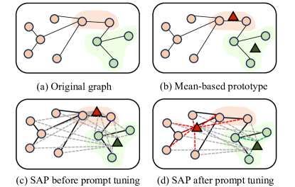
Figure 1. The construction of class prototype vectors. The colored areas contain the labeled nodes for training. The circles represent nodes, and the triangles represent class prototype vectors for node classification task. The solid black lines and gray dashed lines denote the original edges in the graph and the new weighted edges, respectively. For each node, the dashed line in red or green denotes the edges with the largest weight to the class prototype vector.

In this paper, we propose a novel Structure-bAsed Prompting (SAP) method for GNNs, which unifies the objectives of pre-training and prompt tuning for GNNs and integrates structural information in both pre-training and prompt tuning stages. For pre-training, we employ dual-view contrastive learning to align the latent semantic spaces of node attributes and graph structure. Specifically, one view is implemented with MLP, which only uses node attributes in the graph. The other view adopts GNN to leverage both node attributes and structural information of the graph. For downstream prompt-tuning, we fix the learned parameters of MLP and GNN in the pre-training stage, add class prototype vectors as new nodes to the raw graph and introduce structural connections between prototype vectors and original nodes as prompts to learn more accurate prototype vectors (see Figure 1 (c)). Note that weights associated with these connections are parameters to be learned. In the training phase, we use representations of labeled nodes/graphs calculated by MLP as anchors, and representations of prototype vectors obtained through GNN as positive/negative samples. Specifically, the prototype vector in the same class as the anchor is considered as positive sample, while prototype vectors in other classes serve as negative samples. Then, contrastive learning between nodes/graphs (MLP-based view) and prototype vectors (GNN-based view) is performed to learn prompt parameters. As a result, we unify the objectives of pre-training and prompt tuning. After prompt tuning, the nodes and their corresponding class prototypes are learned to have higher weights on the edges, as shown in Figure 1(d). We also experimentally show the results in Figure 6 of Section 5.5. Based on the learned weights, for each prototype vector, GNN formulates its embedding by weighted-aggregating information from its neighboring nodes, i.e., all the nodes in the raw graph. Finally, in the testing stage, node/graph classification can be conducted via comparing the similarity of representations between node/graph and the prototype vectors.

Compared with conventional graph prompt tuning methods, our method is more desirable in learning better prototype vectors, as we leverage both labeled nodes and massive unlabeled nodes in the graph, which is particularly useful in few-shot scenarios. We further highlight that our prompt tuning method is applicable to both homophilous and heterophilous graphs. First, node/graph representations computed from MLP-based view are not affected by structural heterophily. Second, prototype vectors calculated from GNN-based view are based on the learned weights in structure prompt tuning, which takes all nodes in the raw graph as neighbors and learns to assign large (small) weights to those in the same (different) class. As such, the computation of prototype vectors is not affected by the heterophily of the graph. To summarize, our main contributions in this paper are:

• We propose an effective structure-based prompting method SAP for GNNs, which unifies the objectives of pre-training and prompt tuning.

• We present a novel prompt tuning strategy, which introduces a learnable structure prompt to enhance model performance in few-shot learning tasks on both homophilous and heterophilous graphs.

• We extensively demonstrate the effectiveness of SAP with different benchmark datasets on both node classification and graph classification. In particular, we vary the number of labeled training data and show that SAP can lead to better performance in challenging few-shot scenarios.

2. Related work

2.1. Graph Neural Networks

GNNs have presented powerful expressiveness in many graph-based applications (Li et al., 2019; Cheng et al., 2023; Hou et al., 2022; Sun et al., 2021). Modern GNNs typically follow a message-passing scheme, which combines the attribute information and structural information of the graph to derive low-dimensional embedding of a target node by aggregating messages from its context nodes. There are many effective neural network structures proposed such as graph attention network (GAT) (Veličković et al., 2017), graph convolution network (GCN) (Kipf and Welling, 2016), GraphSAGE (Hamilton et al., 2017).

2.2. Graph Pre-training

Inspired by the remarkable achievements of pre-trained models in Natural Language Processing (NLP) (Long et al., 2022; Beltagy et al., 2019; Dong et al., 2019) and Computer Vision (CV) (Qiu et al., 2020b; Bao et al., [n. d.]; Lu et al., 2019), graph pre-training (Xia et al., 2022b) emerges as a powerful paradigm that leverages self-supervision on label-free graphs to learn intrinsic graph properties. Some effective and commonly-used pre-training strategies include node-level comparison  (Zhu et al., 2021), edge-level pretext  (Jin et al., 2020), and graph-level contrastive learning  (You et al., 2020; Xia et al., 2022a). Recently, there are also some newly proposed pre-training methods. For example, GCC (Qiu et al., 2020a) leverages contrastive learning to capture the universal network topological properties across multiple networks and transfers the learned prior knowledge to downstream tasks. GPT-GNN (Hu et al., 2020a) introduces a self-supervised attributed graph generation task to pre-train GNN models that can capture the structural and semantic properties of the graph. L2P-GNN (Lu et al., 2021) utilizes meta-learning to learn the fine-tune strategy during the pre-training process. In summary, there exists a diverse range of pre-training strategies for GNN models, each characterized by unique pre-training objectives. However, these approaches do not consider the gap between pre-training and downstream objectives, which limits their generalization ability to handle different tasks.

2.3. Prompt-based Learning

The training strategy “pre-train & fine-tune” is widely used to adapt pre-trained models onto specific downstream tasks. However, this strategy ignores the inherent gap between the objectives of pre-training and diverse downstream tasks, where the knowledge learned via pre-training could be forgot or ineffectively leveraged for downstream tasks, leading to poor performance.

To bridge this gap, natural language processing proposes a new paradigm (Liu et al., 2023b), namely “pre-train & prompt”. These methods freeze the parameters of the pre-trained models and introduce additional learnable components in the input space, thereby enhancing the compatibility between inputs and pre-trained models. On graph data, there are a handful of studies that adopt prompt tuning to learn more generalizable GNNs. GPPT (Sun et al., 2022) relies on edge prediction as the pre-training task and reformulates the downstream task as edge prediction by introducing task tokens for node classification. GraphPrompt (Liu et al., 2023a) proposes a unified framework based on subgraph similarity and link prediction, hinging on a learnable prompt to actively guide downstream tasks using task-specific aggregation in readout function. SGL-PT (Zhu et al., 2023) unifies the merits of generative and contrastive learning through the asymmetric design as pre-training, and computes class prototype vectors via supervised prototypical contrastive learning (SPCL) (Li et al., 2020; Cui et al., 2022). GPF (Fang et al., 2022) extends the node embeddings with additional task-specific prompt parameters, and can be applied to the pre-trained GNN models that employ any pre-training strategy. ProG (Sun et al., 2023) reformulates node-level and edge-level tasks to graph-level tasks, and introduces the meta-learning technique to the graph prompt tuning study.

Despite their success, we observe that most of them utilize the structure information in pre-training, while ignoring it in downstream prompt tuning stage. This restricts their effectiveness to fully utilize pre-trained knowledge stored in the entire graph. Moreover, their task-specific parameters are usually learned only with few labeled data, leading to poor performance in more challenging few-shot scenarios. In this paper, our proposed method SAP integrates structure information in both pre-training and prompt tuning stage, and achieve superior performance under few-shot setting on both node classification and graph classification tasks.

3. Preliminary

Graph. We denote a graph as $\mathcal{G}=(\mathcal{V},\mathcal{E})$, where $\mathcal{V}=\left\{v_{i}\right\}_{i=1}^{N}$ is a set of $N$ nodes and $\mathcal{E}\subseteq\mathcal{V}\times\mathcal{V}$ is a set of edges. We also define $\mathbf{A}\in\mathbb{R}^{N\times N}$ as the adjacency matrix of $\mathcal{G}$, where $A_{ij}=1$ if $v_{i}$ and $v_{j}$ are connected in $\mathcal{G}$, and $A_{ij}=0$ otherwise. Each node in the graph is associated with an $F$-dimensional feature vector $\mathbf{x}_{i}\in\mathbb{R}^{1\times F}$, and the feature matrix of all nodes is defined as $\mathbf{X}\in\mathbb{R}^{N\times F}$.

Research problem. In this paper, we investigate the problem of graph pre-training and prompt tuning, which learns representations of graph data via pre-training, and transfer the pre-trained knowledge to solve downstream tasks, i.e., node classification and graph classification. Moreover, we further consider the scenarios where downstream tasks are given limited supervision, i.e., $k$-shot classification. For each class, only $k$ labeled samples (i.e., nodes or graphs) are provided as training data.

Prompt tuning of pre-trained models. Given a pre-trained model, a set of learnable prompt parameters $\theta$ and a labeled task dataset $\mathcal{D}$, we fix the parameters of the pre-trained model and only optimize $\theta$ with $\mathcal{D}$ for the downstream graph tasks.

4. Proposed Method

In this paper, we propose a novel structure-based prompting method for GNNs, namely SAP, which unifies the objectives of pre-training and prompt tuning for GNNs and integrates structure information in both pre-training and prompt tuning stage to achieve better performance in more challenging few-shot scenarios. The overall framework of SAP  is shown in Figure 2.

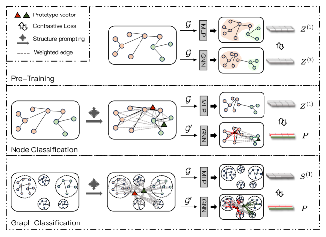
Figure 2. Overall framework of SAP. Top: pre-training. Middle: prompt tuning for node classification. Bottom: prompt tuning for graph classification.

4.1. Graph Pre-training

For graph data, both attribute and structural information are critical for revealing the underlying semantics of graph during the pre-training phase. As such, we design a dual-view contrastive learning to align the latent semantic spaces of node attributes and graph structures. The top part of Figure 2 shows the dual-view pre-training paradigm. In particular, one view is implemented with MLP, which only uses node attributes in the graph, while the other adopts GNN to leverage both node attributes and structural information of the graph. More formally, we define the node representations computed by the two views respectively as

(1) $$\mathbf{Z}^{(1)}=\textrm{MLP}(\mathbf{X})\;\;\;\;\textrm{and}\;\;\;\;\mathbf{Z}^{(2)}=\textrm{GNN}(\mathbf{X},\mathbf{A}),$$

where $\mathbf{Z}^{(1)}\in\mathbb{R}^{N\times D}$ and $\mathbf{Z}^{(2)}\in\mathbb{R}^{N\times D}$ have the same latent dimensionality $D$.

To optimize the MLP and GNN, we leverage a contrastive loss function $\mathcal{L}_{pre}$ to maximize the similarity between the two representations of the same node, denoted as $\mathbf{z}^{(1)}_{i}$ and $\mathbf{z}^{(2)}_{i}$ for node $v_{i}$. For an anchor $\mathbf{z}^{(1)}_{i}$, other node representations $\mathbf{z}^{(2)}_{j}$ are considered as negative samples. More specifically, we formulate the loss as the normalized temperature-scaled cross entropy loss (Chen et al., 2020) as

(2) $$\mathcal{L}_{pre}=-\frac{1}{N}\sum_{i}^{N}\log\frac{\exp(\mathrm{sim}(\mathbf{z}^{(1)}_{i},\mathbf{z}^{(2)}_{i})/\tau)}{{\textstyle\sum_{j=0,j\neq i}^{N}}(\exp(\mathrm{sim}(\mathbf{z}^{(1)}_{i},\mathbf{z}^{(2)}_{j})/\tau))},$$

where $N$ is the number of nodes, $\tau$ is a temperature parameter, and $\textrm{sim}(\cdot)$ is implemented with cosine similarity.

In general, the dual-view contrastive pre-training can exploit both attribute and structure information of graph to encode learning generalizable knowledge in the output node embeddings. In the next subsection, we introduce graph structure prompt tuning that leverage such knowledge in downstream classification tasks.

4.2. Graph Structure Prompt Tuning

Next, we demonstrate how we freeze the pre-trained model and adapt it to different downstream tasks on graph. In particular, we propose a novel method, namely structure prompt tuning, which considers the structure relationships between the graph data and the task at hand. Compared to existing graph prompt tuning methods, the structure relationships in our method allow the task to more effectively leverage the pre-trained knowledge embedded in the graph data. In the following, we elaborate the structure prompt tuning method on two representative tasks, i.e., node classification and graph classification.

4.2.1. Node Classification

The overall framework of our method is similar to previous prototype-based methods (Liu et al., 2023a; Zhu et al., 2023), which learns a prototype embedding vector $\mathbf{p}_{c}$ for each node class $c\in\{1,2,...,C\}$. In particular, our method comprises three steps: 1) structure prompting, 2) prototype initialization, and 3) prompt tuning.

Step 1: Structure prompting. For all the class prototypes, the main idea of our method is to consider them as virtual nodes, and connect them to all the original nodes $\mathcal{V}$ in the graph $\mathcal{G}$, as shown in Figure 1(c). More specifically, we add totally $C$ nodes (denoted as $\mathcal{P}=\left\{p_{c}\right\}_{c=1}^{C}$) and $N\times C$ weighted edges (denoted as $\mathcal{W}$) to construct a prompted graph $\mathcal{G}^{\prime}$ as

(3) $$\mathcal{G}^{\prime}=(\mathcal{G}\cup\mathcal{P},\mathcal{E}\cup\mathcal{W}).$$

Step 2: Prototype initialization. Next, we define the attributes and edge weights for the prototype nodes. In particular, we simply define the attributes for each prototype $p_{c}$ as the averaged attribute vector of its corresponding labeled nodes, i.e.,

(4) $$\mathbf{x}_{c}=\frac{1}{|\mathcal{D}_{c}|}\sum_{(v_{i},c)\in\mathcal{D}_{c}}\mathbf{x}_{i}.$$

For the edges that connect $\mathcal{P}$ and $\mathcal{V}$, we initialize their weights $\mathbf{W}\in\mathbb{R}^{N\times C}$ as

(5) $$\mathbf{W}=\mathbf{Z}^{(2)}\mathbf{P}^{\prime\mathsf{T}}.$$

Here, we introduce a surrogate prototype embedding matrix $\mathbf{P}^{\prime}$, where each row vector $\mathbf{p}_{c}^{\prime}$ of $\mathbf{P}^{\prime}$ is aggregated from its labeled nodes, i.e.,

(6) $$\mathbf{p}_{c}^{\prime}=\frac{1}{|\mathcal{D}_{c}|}\sum_{(v_{i},c)\in\mathcal{D}_{c}}\mathbf{z}^{(2)}_{i}.$$

During the subsequent prompt tuning step, the weight matrix $\mathbf{W}$ is considered as task-specific parameters to be learned.

Step 3: Prompt tuning. We conduct prompt tuning on the prompted graph $\mathcal{G}^{\prime}$ using the same form of loss function as in Equation 2, while keeping the node representations fixed and only optimize the prototypes embeddings. Formally, the prompt tuning loss is defined as the following contrastive loss as

(7) $$\mathcal{L}_{pro}=-\frac{1}{|\mathcal{D}|}\sum_{(v_{i},c)\in\mathcal{D}}\log\frac{\exp(\mathrm{sim}(\mathbf{z}^{(1)}_{i},\mathbf{p}_{c})/\tau)}{\textstyle\sum_{c^{\prime}\in C,c^{\prime}\neq c}\exp(\mathrm{sim}(\mathbf{z}^{(1)}_{i},\mathbf{p}_{c^{\prime}})/\tau)},$$

where $\mathbf{p}_{c}$ is parameterized by $\mathbf{W}$ as

(8) $$\mathbf{P}=\textrm{GNN}([\mathbf{X},\mathbf{X}_{P}],[\mathbf{A},\mathbf{W}]).$$

Here, $\mathbf{X}$ represents the original node features in graph $\mathcal{G}$, $\mathbf{X}_{P}\in\mathbb{R}^{C\times F}$ represents the prototype features, and $[\mathbf{A},\mathbf{W}]\in\mathbb{R}^{N\times(N+C)}$ represents the adjacency matrix of $\mathcal{G}^{\prime}$. Notably, unlike conventional methods that directly consider $\mathbf{P}$ as learnable parameters, we parameterize $\mathbf{P}$ with their structure connections with the graph data, i.e., the added edges $\mathbf{W}$. In other words, only $\mathbf{W}$ would be optimized as parameters when minimizing $\mathcal{L}_{pro}$, which learns to aggregate pre-trained knowledge from all the nodes in the graph to formulate prototype embeddings.

4.2.2. Graph Classification

Our method can also be adopted for graph classification, with some changes to be made in each step. In structure prompting, for each graph instance $\mathcal{G}_{i}$ and a prototype node $p_{c}$, the added edge between any $v_{i}\in\mathcal{V}_{i}$ and $p_{c}$ share the same weight. As such, the prompt tuning of graph classification also has $N\times C$ parameters, while $N$ denotes the number of graphs here. In prototype initialization, we further introduce a mean-based readout function on node level representations $\mathbf{Z}^{(1)}$ and $\mathbf{Z}^{(2)}$ to compute the graph-level representation $\mathbf{S}^{(1)}$ and $\mathbf{S}^{(2)}$, respectively, as shown in Figure 2. Then, we can use Equations 5 and 6 to initialize $\mathbf{W}$ with $\mathbf{Z}^{(2)}$ replaced by $\mathbf{S}^{(2)}$. In prompt tuning, we can also replace $\mathbf{Z}^{(1)}$ replaced by $\mathbf{S}^{(1)}$ in Equation 7 for optimizing graph-level classification tasks.

4.2.3. Remarks

In our proposed SAP method, it worth noting that the weights of pre-trained model are frozen for downstream tasks, and the prompt tuning is parameterized by the learnable adjacency matrix $\mathbf{W}\in\mathbb{R}^{N\times C}$. Compared with most existing studies where the prototype vectors are directly optimized on few labeled data, this allows the prototype vectors to aggregate pre-trained knowledge from massive unlabeled nodes for more effective task adaptation.

4.3. Inference

In the inference stage, classification is performed by comparing the similarity of representations between node/graph (from MLP-based view) and prototype vectors (from GNN-based view) from different classes. The class corresponding to the prototype vector with the largest similarity is taken as the final prediction of the node/graph. We use node classification as an example to explain in detail. By comparing the node representation with each class prototype vector $\mathbf{p}_{c}$, we can get the predicted class probability

(9) $$p(c|v_{i})=\frac{\exp(\mathrm{sim}(\mathbf{z}^{(1)}_{i},\mathbf{p}_{c})/\tau)}{\textstyle\sum_{c=0}^{C}\exp(\mathrm{sim}(\mathbf{z}^{(1)}_{i},\mathbf{p}_{c})/\tau)},$$

where the highest-scored class is chosen as the prediction.

5. Experiments

In this section, we conduct extensive experiments on node classification and graph classification tasks with 10 benchmark datasets to evaluate our proposed SAP.

5.1. Experimental Setup

Datasets. We evaluate the performance of SAP using various benchmark datasets with diverse properties, including homophilous graphs: citation networks (Kipf and Welling, 2016) (i.e, Cora, CiteSeer, PubMed), ogbn-arxiv (Hu et al., 2020b), and heterophilous graphs: Chameleon (Pei et al., 2020), Actor (Pei et al., 2020), ENZYMES (Wang et al., 2022), PROTEINS (Borgwardt et al., 2005), COX2 (Rossi and Ahmed, 2015), BZR (Rossi and Ahmed, 2015). We summarize these datasets in Table 1. Note that the “Task” column indicates the type of downstream task on each dataset, where “N” represents node classification and “G” represents graph classification.

Table 1. Statistics of the datasets.

Datasets	Graphs	Graph	Avg.	Avg.	Node	Node	Task
		classes	nodes	edges	features	classes	(N/G)
Cora	1	-	2,708	5,429	1433	7	N
CiteSeer	1	-	3,327	4,732	3703	6	N
PubMed	1	-	19,717	44,338	500	3	N
ogbn-arxiv	1	-	169,343	1,166,243	128	40	N
Chameleon	1	-	2,277	31,421	2325	5	N
Actor	1	-	7,600	26,752	931	5	N
ENZYMES	600	6	32.63	62.14	18	3	N, G
PROTEINS	1,113	2	39.06	72.82	1	3	G
COX2	467	2	41.22	43.45	3	-	G
BZR	405	2	35.75	38.36	3	-	G

Baselines. To evaluate the proposed SAP, we compare it with 3 categories of state-of-the-art approaches as follows.

• Supervised models: GraphSAGE (Hamilton et al., 2017), GCN (Kipf and Welling, 2016) and GAT (Veličković et al., 2017). They use the labeled data to learn GNNs, which are then directly applied for the classification tasks.

• Graph pre-training models: EdgeMask (Veličković et al., 2018) and GraphCL (You et al., 2020). Following the transfer learning strategy of “pre-train & fine-tune”, the pre-trained models are fine-tuned on the downstream tasks.

• Graph prompt models: GPPT (Sun et al., 2022), GraphPrompt (Liu et al., 2023a), GPF (Fang et al., 2022) and ProG (Sun et al., 2023). They adopt the “pre-train & prompt” paradigm, where the pre-trained models are frozen, and task-specific learnable prompts are introduced and trained in the downstream tasks. Note that GPF works for all pre-training tasks, in our experiments GraphCL is used for pre-training.

Table 2. Accuracy (%) on node classification. We highlight the best score on each dataset in bold.

Methods	Supervised			Pre-train		Prompt				Ours
	GraphSAGE	GCN	GAT	EdgeMask	GraphCL	GPPT	GraphPrompt	GPF	ProG	SAP
Masking ratio = 0%
Cora	81.07(0.30)	76.32(0.95)	78.47(1.68)	81.00(0.93)	81.05(0.59)	81.40(0.48)	72.15(0.51)	69.44(0.41)	78.29(0.47)	80.32(0.35)
CiteSeer	67.95(0.34)	65.40(0.13)	65.61(0.57)	67.39(0.98)	68.03(0.71)	69.21(0.48)	67.62(0.50)	64.12(0.39)	70.05(0.54)	72.23(0.42)
PubMed	77.24(0.62)	75.33(0.27)	75.91(0.14)	78.51(0.14)	79.10(0.52)	79.73(0.38)	77.90(0.34)	77.08(0.41)	76.82(0.31)	82.04(0.28)
ogbn-arxiv	65.07(0.67)	64.26(0.15)	64.31(1.06)	65.59(0.18)	67.34(0.92)	65.94(0.24)	59.25(0.31)	57.02(0.34)	70.49(0.21)	72.63(0.67)
Chameleon	32.85(1.21)	36.60(0.61)	34.69(0.72)	31.62(0.38)	29.30(0.16)	34.25(0.81)	35.11(0.23)	32.47(1.92)	36.68(1.25)	37.94(0.68)
Actor	22.57(0.83)	20.98(1.00)	21.98(0.24)	22.83(0.90)	23.17(1.07)	25.17(0.82)	22.62(0.96)	23.70(0.71)	24.79(1.01)	28.80(0.48)
Masking ratio = 30%
Cora	75.51(0.73)	74.04(0.30)	76.00(0.51)	76.32(0.32)	76.72(0.36)	76.83(0.26)	67.34(0.37)	61.72(0.28)	73.27(0.53)	77.05(0.40)
CiteSeer	64.46(0.56)	56.05(0.56)	61.23(0.60)	63.71(0.46)	63.98(0.54)	64.74(0.17)	63.96(0.31)	62.99(0.48)	65.02(0.47)	68.78(0.23)
PubMed	77.79(0.34)	78.12(0.64)	77.40(0.63)	79.30(0.48)	79.01(0.61)	80.15(0.34)	78.13(0.47)	71.49(0.25)	74.23(0.36)	80.21(0.31)
ogbn-arxiv	65.69(0.23)	63.18(0.38)	64.32(0.25)	65.99(0.69)	65.72(0.37)	66.18(0.33)	60.25(0.42)	56.68(0.39)	69.84(0.49)	71.96(0.97)
Chameleon	32.82(0.73)	35.01(0.42)	33.69(0.36)	31.02(0.57)	31.58(0.10)	34.31(0.95)	33.61(0.14)	30.62(1.67)	35.28(0.94)	39.20(0.29)
Actor	21.28(0.79)	20.71(0.47)	21.03(0.51)	22.94(0.85)	23.28(0.07)	24.76(0.49)	21.90(0.22)	23.25(0.29)	24.10(0.93)	26.64(1.03)
Masking ratio = 50%
Cora	68.40(0.96)	71.78(0.50)	74.94(1.26)	76.38(0.89)	76.73(0.91)	77.16(1.35)	68.43(0.58)	62.20(0.93)	72.49(1.04)	77.62(1.29)
CiteSeer	57.98(0.98)	52.15(0.27)	59.50(0.61)	65.49(0.90)	65.94(1.20)	65.81(0.97)	61.11(1.24)	60.78(1.17)	65.33(0.93)	67.52(0.95)
PubMed	68.23(0.46)	65.05(0.15)	69.30(0.97)	71.29(0.66)	72.03(1.54)	72.23(1.22)	72.63(1.72)	68.81(0.95)	73.70(1.49)	75.94(1.06)
ogbn-arxiv	64.56(0.75)	64.19(0.59)	63.97(0.69)	64.86(0.67)	65.87(0.82)	66.13(0.44)	59.13(0.59)	56.04(0.97)	67.80(1.65)	69.20(0.73)
Chameleon	27.93(1.72)	30.38(1.21)	29.14(0.79)	30.89(1.15)	27.37(1.40)	31.28(0.65)	31.67(1.19)	29.31(1.68)	31.75(1.25)	34.08(1.26)
Actor	19.13(0.85)	18.67(1.94)	20.85(1.37)	21.76(0.95)	22.18(1.24)	22.07(0.81)	21.11(1.35)	20.56(1.09)	22.82(1.03)	25.47(0.82)

Implementation details. To train SAP, we adopt the Adam optimizer (Kingma and Ba, 2014), where the learning rate and weight decay in the pre-training stage is fixed as 1e-4. We set the number of both graph neural layers and multilayer perceptron layers as 2. We set the hidden dimension for node classification as 128, and for graph classification as 32. Other hyper-parameters are tuned on the results on the validation set by a grid search. Details of the hyper-parameter setting is listed in Appendix C. Furthermore, for those non-prompt-based competitors, some of their results are directly reported as in (Sun et al., 2022) and (Liu et al., 2023a) (i.e., node classification with 0%, 30% and 50% masking ratio and graph classification). For other cases and prompt-based models, we fine-tune hyper-parameters with the codes released by their original authors. For fair comparison, we report the average results with standard deviations of 5 runs for node classification experiments, while the setting of graph classification experiments follow (Liu et al., 2023a). We run all the experiments on a server with 32G memory and a single Tesla V100 GPU.

5.2. Node classification

Experimental setting. We conduct node classification on 6 datasets, i.e., Cora, CiteSeer, PubMed, ogb-arxiv, Chameleon and Actor. For homophilous graph datasets, we use the official splitting of training/validation/testing (Kipf and Welling, 2016). For heterophilous graph datasets, we randomly sample 20 nodes per class as training set and validation set, respectively. The remaining nodes which are not sampled will be used for evaluation. Following the setting of (Sun et al., 2022), we randomly mask 0%, 30% and 50% of the training labels. Note that for datasets except ogbn-arxiv, the masking ratio of 0%, 30% and 50% correspond to 20-shot, 14-shot and 10-shot.

Results. Table 2 summarizes the performance results, from which we make the following major observations.

(1) Most supervised methods are very hard to achieve better performance compared with pre-training methods and prompt methods. This is because the annotations required by supervised frameworks are not enough. In contrast, pre-training approaches are usually facilitated with more prior knowledge, alleviating the need for labeled data. However, these pre-training methods still face an inherent gap between the training objectives of pre-training and downstream tasks. Pre-trained models may suffer from catastrophic forgetting during downstream adaptation. Therefore, we can find that compared with pre-training approaches, prompt-based methods usually achieve better performance.

(2) In all cases except for 0% mask on Cora, our proposed SAP outperforms all the baselines on node classification. This is because SAP bridges the gap between the pre-training stage and the down-stream prompt tuning stage, and leverages graph structure prompt to provide more information from the massive unlabeled nodes. Specifically, we add class prototype vectors as new nodes to the raw graph and introduce weighted edges between prototype vectors and original nodes as prompts.

Table 3. Accuracy (%) on few-shot node classification.

Methods	Supervised			Pre-train		Prompt				Ours
	GraphSAGE	GCN	GAT	EdgeMask	GraphCL	GPPT	GraphPrompt	GPF	ProG	SAP
Cora	56.28(3.17)	57.83(5.90)	60.34(4.15)	64.10(2.79)	65.89(3.45)	64.55(3.72)	63.91(2.43)	63.52(5.39)	65.68(4.29)	68.65(2.17)
CiteSeer	52.71(3.28)	49.69(4.39)	52.85(3.69)	55.23(3.17)	58.37(4.74)	55.63(2.55)	53.42(4.98)	54.31(5.21)	59.07(2.73)	61.70(4.21)
PubMed	63.83(4.21)	63.16(4.56)	64.26(3.17)	65.89(4.26)	69.06(3.24)	70.07(6.07)	68.93(3.93)	63.98(3.54)	64.57(3.81)	72.23(4.20)
ENZYMES	60.02(3.72)	61.49(12.87)	59.94(2.86)	56.17(14.39)	58.73(16.47)	53.79(17.46)	67.04(11.48)	60.13(15.37)	57.22(17.41)	72.86(14.58)
Chameleon	25.69(4.82)	27.88(5.77)	26.97(4.85)	23.76(3.74)	22.25(3.14)	28.91(3.23)	26.35(3.50)	27.38(3.62)	29.18(4.53)	33.23(3.80)
Actor	21.17(3.15)	20.69(2.96)	20.93(2.67)	18.03(2.48)	19.56(1.15)	20.88(1.69)	20.50(2.45)	19.32(2.52)	21.43(3.27)	24.74(2.79)

5.3. Few-shot node classification

Experimental setting. To explore more challenging few-shot node classification settings, we only assign a very smaller number of labeled data as the training data for each class. Specifically, for ENZYMES, we follow existing study (Liu et al., 2023a) to only choose graphs that consist of more than 50 nodes, which ensures there are sufficient labeled nodes for testing. On each graph, we randomly sample 1 node per class for training and validation, respectively. The remaining nodes which are not sampled will be used for testing. For Cora, CiteSeer and PubMed, we randomly sample 3 nodes per class for training, while the validation and test sets follow the official splitting (Kipf and Welling, 2016). For Chameleon and Actor, we randomly sample 3 nodes per class for training and validation respectively, while the remaining nodes which are not sampled are used for testing.

Results. Table 3 illustrates the results. From it, we see that

(1) Compared with the results of 10-shot in Table 2, SAP under this few-shot setting improves more than the baselines. Taking Cora as an example, the accuracy of SAP is 0.46% higher than the runner-up under 10-shot, while under 3-shot, the accuracy of SAP is 2.97% higher than the runner-up. This is because SAP uses graph structure information to optimize the prototype vectors, so when the training set is extremely small, the prototype vectors can also be accurate by capturing the underlying information of other unlabeled nodes. In contrast, other methods fail to consider the relationship between the task and the massive unlabeled data.

(2) Our proposed SAP achieves larger improvements in heterophilous graphs. SAP achieves a largest improvement of 2.97% in homogeneous graphs while 5.82% in heterophilous graphs. This is because in the downstream prompt tuning stage of SAP, node representations computed from MLP-based view are not affected by the structural heterophily. Also, the graph structure prompt reduces the heterophily of the graph. Therefore, the prototype vector representations calculated from GNN-based view are more accurate. In contrast, other methods are susceptible to structure heterophily and can only achieve sub-optimal results.

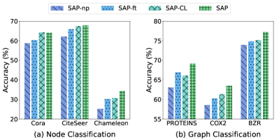
Figure 3. The ablation study on training paradigm.

5.4. Few-shot graph classification

We conduct few-shot graph classification on 4 datasets, i.e., ENZYMES, PROTEINS, COX2 and BZR. Following the setting of (Liu et al., 2023a), we conduct 5-shot tasks. The results are listed in Table 4, from which we observe that our proposed SAP significantly outperforms the baselines on these datasets. This again demonstrates the effectiveness of our proposed method. Notably, as both node and graph classification tasks share the same pre-trained model on ENZYMES, the superior performance of SAP on both types of tasks further demonstrates that the gap between different tasks is better addressed by our unified framework.

Table 4. Accuracy (%) on graph classification.

Methods	ENZYMES	PROTEINS	COX2	BZR
GraphSAGE	18.31$\pm$6.22	52.99$\pm$10.57	52.87$\pm$11.46	57.23$\pm$10.95
GCN	20.37$\pm$5.24	54.87$\pm$11.20	51.37$\pm$11.06	56.16$\pm$11.07
GAT	15.90$\pm$4.13	48.78$\pm$18.46	51.20$\pm$27.93	53.19$\pm$20.61
InfoGraph	20.90$\pm$3.32	54.12$\pm$8.20	54.04$\pm$9.45	57.57$\pm$9.93
GraphCL	28.11$\pm$4.00	56.38$\pm$7.24	55.40$\pm$12.04	59.22$\pm$7.42
GPPT	-	-	-	-
GraphPrompt	31.45$\pm$4.32	64.42$\pm$4.37	59.21$\pm$6.82	61.63$\pm$7.68
GPF	32.65$\pm$5.73	57.16$\pm$5.96	61.62$\pm$7.47	59.17$\pm$6.18
ProG	29.18$\pm$3.09	60.98$\pm$7.49	61.96$\pm$6.35	63.71$\pm$5.25
SAP	33.57$\pm$4.72	64.95$\pm$5.86	65.71$\pm$5.34	68.58$\pm$7.57

5.5. Model Analysis

We further analyse several aspects of our model. The following experiments are conducted on the 3-shot node classification and 5-shot graph classification.

Table 5. Varying the ratio of added edges on few-shot node classification. The $\downarrow$/$\uparrow$ arrow means the decreasing/improvement compared with the accuracy of runner-up.

	runner-up	0%	0.1%	1%	5%	10%	30%	50%	100%
Cora	65.89$\pm$3.45	65.06$\pm$3.77 $\downarrow$	65.72$\pm$3.14 $\downarrow$	67.50$\pm$2.38 $\uparrow$	67.46$\pm$2.45 $\uparrow$	67.88$\pm$2.83 $\uparrow$	67.56$\pm$3.19 $\uparrow$	68.62$\pm$2.67 $\uparrow$	68.68$\pm$2.17 $\uparrow$
CiteSeer	59.07$\pm$2.73	56.70$\pm$4.16 $\downarrow$	57.03$\pm$5.25 $\downarrow$	57.52$\pm$5.03 $\downarrow$	59.36$\pm$5.90 $\uparrow$	60.98$\pm$4.98 $\uparrow$	61.44$\pm$3.96 $\uparrow$	62.62$\pm$4.26 $\uparrow$	62.76$\pm$4.21 $\uparrow$
PubMed	70.07$\pm$6.07	70.84$\pm$5.31 $\uparrow$	70.32$\pm$3.95 $\uparrow$	71.62$\pm$4.34 $\uparrow$	70.94$\pm$4.40 $\uparrow$	71.42$\pm$4.70 $\uparrow$	72.20$\pm$4.62 $\uparrow$	72.24$\pm$4.33 $\uparrow$	73.23$\pm$4.20 $\uparrow$
Chameleon	29.18$\pm$4.53	25.22$\pm$3.09 $\downarrow$	30.92$\pm$3.07 $\uparrow$	33.41$\pm$3.38 $\uparrow$	33.30$\pm$2.36 $\uparrow$	33.07$\pm$3.79 $\uparrow$	31.89$\pm$3.83 $\uparrow$	32.09$\pm$2.20 $\uparrow$	33.97$\pm$3.22 $\uparrow$

Ablation study on training paradigm. We conduct an ablation study that compares variants of SAP with different pre-training and prompt tuning strategies: (1) We directly fine-tune the pre-trained models (i.e., MLP and GNN) on the tasks, instead of prompt tuning. We call this variant SAP-ft (with fine-tune). (2) For downstream tasks, we remove the prompt tuning process and only use the mean embedding vectors of the labeled data as the prototype vectors to perform classification. We call this variant SAP-np (no prompt). (3) We replace our proposed dual-view contrastive learning in pre-training with GraphCL, i.e., the pre-trained encoder is GNN, while the downstream tasks still use our proposed graph structure prompt. We call this variant SAP-CL (with GraphCL as the pre-training model). Figure 3 shows the results of this study, where we have the following observations:

(1) SAP-np always performs the worst among all the variants, showing the effectiveness of our proposed graph structure prompt. SAP-ft achieves better performance than SAP-np, which is because SAP-ft is parameterized.

(2) SAP achieves comparable results to SAP-CL in homogeneous graph datasets and clearly outperforms SAP-CL in heterophilous graph datasets. This is because our pre-training method uses MLP and GNN for contrastive learning, where MLP is not affected by the heterophily of the graph. In contrast, SAP-CL is susceptible to structure heterophily and can only achieve sub-optimal result in heterophilous graph datasets.

Varying the number of the shots. We next vary the number of shots on two datasets for node classification (Cora, CiteSeer) and graph classification (PROTEINS and COX2), respectively. For node classification, we vary the number of shots between 1 and 10. For graph classification, we vary the number of shots between 1 and 30. We compare SAP with several competitive baselines in Figure 4 and 5. In general, SAP consistently outperforms the baselines, especially when the number of shots is few. We further notice that when the number of shots is relatively large, SAP can be surpassed by graphCL on graph classification, especially on COX2. This could be contributed to more available training data on COX2, where 30 shots per class implies that 12.85% of the 467 graphs are used for training. This is not our target few-shot scenario.

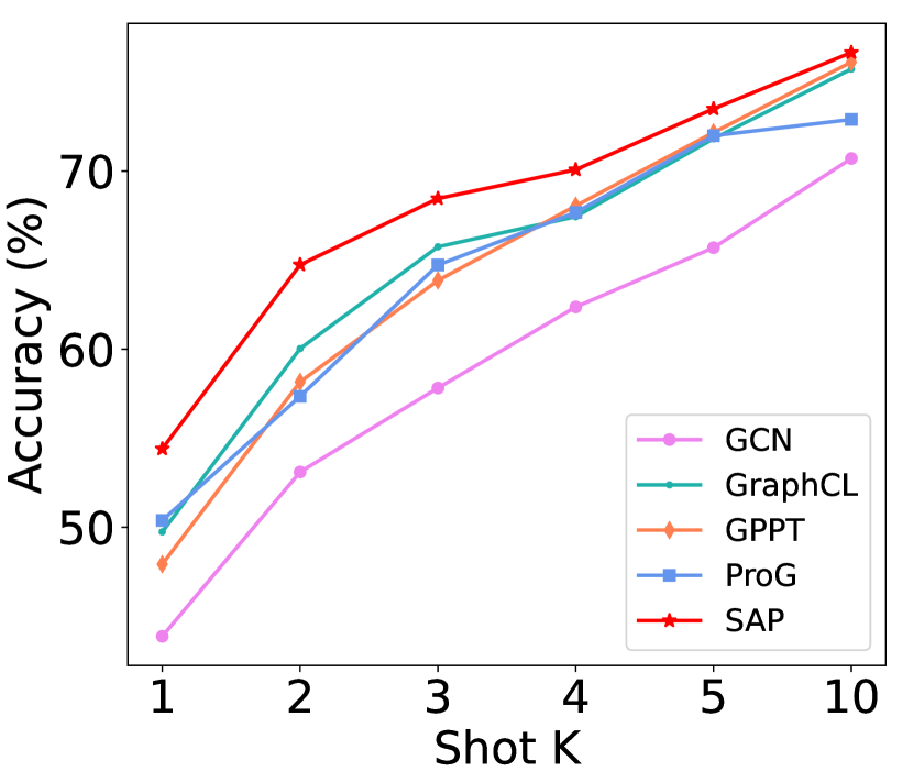
(a) Cora

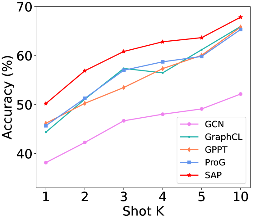
(b) CiteSeer

Figure 4. Varying the number of shots for node classification.

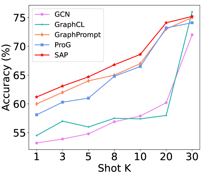
(a) PROTEINS

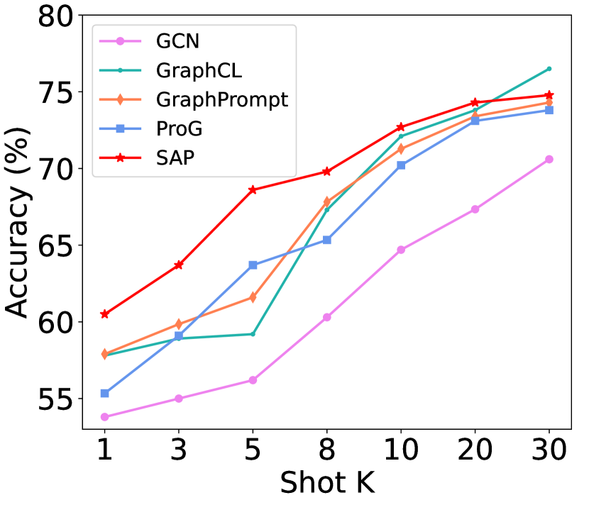
(b) COX2

Figure 5. Varying the number of shots for graph classification.

Varying the ratio of added edges. Our prompt tuning method is parameterized by the added edges between original nodes and prototype vectors, where the weights of added edges are learnable. We hereby study the impact of the ratio of added edges (i.e., parameters) $r$. To vary the number of edges, we first randomly select $Nr$ nodes outside the training set. During prompt tuning, we next merge the $Nr$ nodes with $N_{t}$ training nodes as the set of nodes to build edges with all the $C$ prototypes. Following this setting, we conduct 3-shot node classification on 4 datasets. The results are shown in Table 5. Surprisingly, we observe that for Cora, CiteSeer and Chameleon, SAP only needs 1%, 5% and 0.1% parameters, respectively to surpass the runner-up. For PubMed, SAP can outperform runner-up only using the training set. This proves that our prompt tuning model can achieve comparable performance with only a small number of parameters $(N_{t}+Nr)C$, As such, SAP is promising in scaling to large graphs.

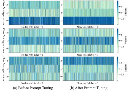
Figure 6. The weights of added edges between nodes and class prototype vectors before and after prompt tuning.

Visualization of learned edge weights. We visualize the weight matrix $\mathbf{W}$ of the added edges after prompt tuning. As shown in Figure 6, for each node, its edge connected to its corresponding class prototype is more likely to have a larger weight. Hence, the prototype vectors are very accurate by aggregating massive unlabeled data which contain rich pre-trained knowledge to reflect the semantics of the task labels.

Time complexity analysis. The major time complexity in our proposed SAP comes from MLP, GNN and the contrastive loss. We take node classification as an example. Suppose we use one-layer MLP and GCN as the backbone, since the adjacency matrix is generally sparse, let $d_{A}$ be the average number of non-zero entries in each row of the adjacency matrix $\mathbf{A}$. Let $N$ be the number of nodes, $F$ be the dimensionality of raw features, $D$ be the dimensionality of output layer and $C$ be the number of class labels. Then, the time complexities for MLP and GCN are $O(NFD)$ and $O(Nd_{A}F+NFD)$, respectively. We next analyze the time complexity of the contrastive loss. In the pre-training stage, let $M$ be the number of selected negative samples. The time complexity is $O(NMD)$, which is linear to the number of nodes $N$. Then we conduct $C$-way $K$-shot learning for downstream tasks. For each node, we need to calculate its similarity with all prototype vectors, so the time complexity is $O(CD)$. In the prompt tuning stage, we have a total of $KC$ labeled nodes for training, so the time complexity is $O(KC^{2}D)$. In the inference stage, the time complexity is $O(CD)$.

6. conclusion

In this paper, we proposed SAP, a novel structure-based prompting method for GNNs, which unifies the objectives of pre-training and prompt tuning for GNNs and integrates structural information in both pre-training and prompt tuning stages. For pre-training, we proposed a dual-view contrastive learning to align the latent semantic spaces of node attributes and graph structure. For downstream prompt tuning, we proposed to learn the structural connection between the prototype vectors and the graph, and then leveraged the learned structural information to perform better in few-shot tasks. Finally, we conducted extensive experiments on 10 public datasets, and showed that SAP significantly outperforms various state-of-the-art baselines on both homophilous and heterophilous graphs, especially on few-shot scenarios.

Appendix A Further Descriptions of Datasets

In this section, we provide further details of the datasets.

• Cora, CiteSeer, and PubMed (Kipf and Welling, 2016) are three citation network datasets. Each of them represents an undirected graph where nodes correspond to documents (academic papers) and edges denote citation relationships. Node features in these datasets are represented as word vectors, with each element being a binary variable, indicating the presence or absence of each word in a paper. The text preprocessing includes stemming and stop word removal, with the exclusion of words that appear in fewer than ten documents. The nodes of Cora, CiteSeer and PubMed belong to 7, 6 and 3 classes, respectively.

• Ogbn-arxiv (Hu et al., 2020b) is a directed graph, representing the citation network between all Computer Science arXiv papers indexed by MAG (Wang et al., 2020). Each node is an arXiv paper and each directed edge indicates that one paper cites another one. Each paper comes with a 128-dimensional feature vector obtained by averaging the embeddings of words in its title and abstract. The embeddings of individual words are computed by running the skip-gram model (Mikolov et al., 2013) over the MAG corpus. The nodes belong to 40 classes.

• Chameleon (Pei et al., 2020) is designed to simulate a network of blog authors who are connected based on their interests and affiliations. In this network, nodes correspond to authors, and edges represent connections between authors who write about similar topics or belong to the same blogging community. The nodes belong to 5 categories.

• Actor (Pei et al., 2020) focuses on social networks. It models the interactions among actors in the film industry, where nodes represent actors, and edges denote co-starring relationships in movies. The nodes belong to 5 categories.

• ENZYMES (Wang et al., 2022) is a dataset of 600 enzymes collected from the BRENDA enzyme database. These enzymes are labeled into 6 categories according to their top-level EC enzyme and the nodes of ENZYMES belong to 3 classes.

• PROTEINS (Borgwardt et al., 2005) is a collection of protein graphs which include the amino acid sequence, conformation, structure, and features such as active sites of the proteins. The nodes represent the secondary structures, and each edge depicts the neighboring relation in the amino-acid sequence or in 3D space. The graphs belong to 2 classes.

• COX2 (Rossi and Ahmed, 2015) is a dataset of molecular structures including 467 cyclooxygenase-2 inhibitors, in which each node is an atom, and each edge represents the chemical bond between atoms, such as single, double, triple or aromatic. All the molecules belong to 2 categories.

• BZR (Rossi and Ahmed, 2015) is a collection of 405 ligands for benzodiazepine receptor, in which each ligand is represented by a graph. All these ligands belong to 2 categories.

Appendix B Further Descriptions of Baselines

In this section, we present more details for the baselines, which are chosen from 3 main categories.

(1) Supervised models.

• GCN (Kipf and Welling, 2016): GCN resorts to mean-pooling based neighborhood aggregation to receive messages from the neighboring nodes for node representation learning in an end-to-end manner.

• GraphSage (Hamilton et al., 2017): GraphSAGE has a similar neighborhood aggregation mechanism with GCN, while it focuses more on the information from the node itself.

• GAT (Veličković et al., 2017): GAT also depends on neighborhood aggregation for node representation learning in an end-to-end manner, while it can assign different weights to neighbors to reweigh their contributions.

(2) Graph pre-training models.

• EdgeMask (Veličković et al., 2018): EdgeMask randomly masks some edges and then the model is asked to reconstruct the masked edges in the graph.

• GraphCL (You et al., 2020): GraphCL applies different graph augmentations to exploit the structural information on the graphs, and aims to maximize the agreement between different augmentations for graph pre-training.

(3) Graph prompt models.

• GPPT (Sun et al., 2022): GPPT pre-trains a GNN model based on the link prediction task, and employs a learnable prompt to reformulate the downstream node classification task into the same format as link prediction.

• GraphPrompt (Liu et al., 2023a): GraphPrompt pre-trains a GNN model based on subgraph similarity and link prediction, hinging on a learnable prompt to actively guide downstream tasks using task-specific aggregation in readout function.

• GPF (Fang et al., 2022): GPF extends the node embeddings with additional task-specific prompt parameters, and can be applied to the pre-trained GNN models that employ any pre-training strategy.

• ProG (Sun et al., 2023): ProG reformulates node-level and edge-level tasks to graph-level tasks, and introduces the meta-learning technique to the graph prompt tuning study.

Appendix C Hyper-parameters settings

We perform grid search to fine-tune hyper-parameters based on the results on the validation set. Details of these hyper-parameters are listed in Table 6.

Table 6. Grid search space.

Notation	Range
learning_rate	{1e-4, 1e-3, 1e-2, 1e-1}
weight_decay	{1e-5, 1e-4, 1e-3, 1e-2}
dropout	[0.2, 0.8]

References

- (1)
- Bao et al. ([n. d.]) H Bao, L Dong, and F Wei. [n. d.]. Beit: Bert pre-training of image transformers. arXiv 2021. arXiv preprint arXiv:2106.08254 ([n. d.]).
- Beltagy et al. (2019) Iz Beltagy, Kyle Lo, and Arman Cohan. 2019. SciBERT: A pretrained language model for scientific text. arXiv preprint arXiv:1903.10676 (2019).
- Borgwardt et al. (2005) Karsten M Borgwardt, Cheng Soon Ong, Stefan Schönauer, SVN Vishwanathan, Alex J Smola, and Hans-Peter Kriegel. 2005. Protein function prediction via graph kernels. Bioinformatics 21, suppl_1 (2005), i47–i56.
- Chen et al. (2020) Ting Chen, Simon Kornblith, Mohammad Norouzi, and Geoffrey Hinton. 2020. A simple framework for contrastive learning of visual representations. In International conference on machine learning. PMLR, 1597–1607.
- Cheng et al. (2023) Jiashun Cheng, Man Li, Jia Li, and Fugee Tsung. 2023. Wiener Graph Deconvolutional Network Improves Graph Self-Supervised Learning. (2023).
- Cui et al. (2022) Ganqu Cui, Shengding Hu, Ning Ding, Longtao Huang, and Zhiyuan Liu. 2022. Prototypical verbalizer for prompt-based few-shot tuning. arXiv preprint arXiv:2203.09770 (2022).
- Dong et al. (2019) Li Dong, Nan Yang, Wenhui Wang, Furu Wei, Xiaodong Liu, Yu Wang, Jianfeng Gao, Ming Zhou, and Hsiao-Wuen Hon. 2019. Unified language model pre-training for natural language understanding and generation. Advances in neural information processing systems 32 (2019).
- Fang et al. (2022) Taoran Fang, Yunchao Zhang, Yang Yang, Chunping Wang, and Lei Chen. 2022. Universal Prompt Tuning for Graph Neural Networks. arXiv preprint arXiv:2209.15240 (2022).
- Hamilton et al. (2017) Will Hamilton, Zhitao Ying, and Jure Leskovec. 2017. Inductive representation learning on large graphs. Advances in neural information processing systems 30 (2017).
- Hou et al. (2022) Zhenyu Hou, Xiao Liu, Yukuo Cen, Yuxiao Dong, Hongxia Yang, Chunjie Wang, and Jie Tang. 2022. Graphmae: Self-supervised masked graph autoencoders. In Proceedings of the 28th ACM SIGKDD Conference on Knowledge Discovery and Data Mining. 594–604.
- Hu et al. (2020b) Weihua Hu, Matthias Fey, Marinka Zitnik, Yuxiao Dong, Hongyu Ren, Bowen Liu, Michele Catasta, and Jure Leskovec. 2020b. Open graph benchmark: Datasets for machine learning on graphs. Advances in neural information processing systems 33 (2020), 22118–22133.
- Hu et al. (2020a) Ziniu Hu, Yuxiao Dong, Kuansan Wang, Kai-Wei Chang, and Yizhou Sun. 2020a. Gpt-gnn: Generative pre-training of graph neural networks. In Proceedings of the 26th ACM SIGKDD International Conference on Knowledge Discovery & Data Mining. 1857–1867.
- Jin et al. (2020) Wei Jin, Tyler Derr, Haochen Liu, Yiqi Wang, Suhang Wang, Zitao Liu, and Jiliang Tang. 2020. Self-supervised learning on graphs: Deep insights and new direction. arXiv preprint arXiv:2006.10141 (2020).
- Kingma and Ba (2014) Diederik P Kingma and Jimmy Ba. 2014. Adam: A method for stochastic optimization. arXiv preprint arXiv:1412.6980 (2014).
- Kipf and Welling (2016) Thomas N Kipf and Max Welling. 2016. Semi-supervised classification with graph convolutional networks. arXiv preprint arXiv:1609.02907 (2016).
- Li et al. (2019) Jia Li, Zhichao Han, Hong Cheng, Jiao Su, Pengyun Wang, Jianfeng Zhang, and Lujia Pan. 2019. Predicting path failure in time-evolving graphs. In Proceedings of the 25th ACM SIGKDD international conference on knowledge discovery & data mining. 1279–1289.
- Li et al. (2020) Junnan Li, Pan Zhou, Caiming Xiong, and Steven CH Hoi. 2020. Prototypical contrastive learning of unsupervised representations. arXiv preprint arXiv:2005.04966 (2020).
- Li et al. (2021) Pengyong Li, Jun Wang, Yixuan Qiao, Hao Chen, Yihuan Yu, Xiaojun Yao, Peng Gao, Guotong Xie, and Sen Song. 2021. An effective self-supervised framework for learning expressive molecular global representations to drug discovery. Briefings in Bioinformatics 22, 6 (2021), bbab109.
- Li et al. (2023) Xiang Li, Tiandi Ye, Caihua Shan, Dongsheng Li, and Ming Gao. 2023. SeeGera: Self-supervised Semi-implicit Graph Variational Auto-encoders with Masking. In Proceedings of the ACM Web Conference 2023. 143–153.
- Liu et al. (2023b) Pengfei Liu, Weizhe Yuan, Jinlan Fu, Zhengbao Jiang, Hiroaki Hayashi, and Graham Neubig. 2023b. Pre-train, prompt, and predict: A systematic survey of prompting methods in natural language processing. Comput. Surveys 55, 9 (2023), 1–35.
- Liu et al. (2023a) Zemin Liu, Xingtong Yu, Yuan Fang, and Xinming Zhang. 2023a. Graphprompt: Unifying pre-training and downstream tasks for graph neural networks. In Proceedings of the ACM Web Conference 2023. 417–428.
- Long et al. (2022) Siqu Long, Feiqi Cao, Soyeon Caren Han, and Haiqin Yang. 2022. Vision-and-language pretrained models: A survey. arXiv preprint arXiv:2204.07356 (2022).
- Lu et al. (2019) Jiasen Lu, Dhruv Batra, Devi Parikh, and Stefan Lee. 2019. Vilbert: Pretraining task-agnostic visiolinguistic representations for vision-and-language tasks. Advances in neural information processing systems 32 (2019).
- Lu et al. (2021) Yuanfu Lu, Xunqiang Jiang, Yuan Fang, and Chuan Shi. 2021. Learning to pre-train graph neural networks. In Proceedings of the AAAI conference on artificial intelligence, Vol. 35. 4276–4284.
- Mikolov et al. (2013) Tomas Mikolov, Ilya Sutskever, Kai Chen, Greg S Corrado, and Jeff Dean. 2013. Distributed representations of words and phrases and their compositionality. Advances in neural information processing systems 26 (2013).
- Pei et al. (2020) Hongbin Pei, Bingzhe Wei, Kevin Chen-Chuan Chang, Yu Lei, and Bo Yang. 2020. Geom-gcn: Geometric graph convolutional networks. arXiv preprint arXiv:2002.05287 (2020).
- Qiu et al. (2020a) Jiezhong Qiu, Qibin Chen, Yuxiao Dong, Jing Zhang, Hongxia Yang, Ming Ding, Kuansan Wang, and Jie Tang. 2020a. Gcc: Graph contrastive coding for graph neural network pre-training. In Proceedings of the 26th ACM SIGKDD international conference on knowledge discovery & data mining. 1150–1160.
- Qiu et al. (2020b) Xipeng Qiu, Tianxiang Sun, Yige Xu, Yunfan Shao, Ning Dai, and Xuanjing Huang. 2020b. Pre-trained models for natural language processing: A survey. Science China Technological Sciences 63, 10 (2020), 1872–1897.
- Rossi and Ahmed (2015) Ryan Rossi and Nesreen Ahmed. 2015. The network data repository with interactive graph analytics and visualization. In Proceedings of the AAAI conference on artificial intelligence, Vol. 29.
- Sun et al. (2022) Mingchen Sun, Kaixiong Zhou, Xin He, Ying Wang, and Xin Wang. 2022. Gppt: Graph pre-training and prompt tuning to generalize graph neural networks. In Proceedings of the 28th ACM SIGKDD Conference on Knowledge Discovery and Data Mining. 1717–1727.
- Sun et al. (2023) Xiangguo Sun, Hong Cheng, Jia Li, Bo Liu, and Jihong Guan. 2023. All in One: Multi-Task Prompting for Graph Neural Networks. (2023).
- Sun et al. (2021) Xiangguo Sun, Hongzhi Yin, Bo Liu, Hongxu Chen, Qing Meng, Wang Han, and Jiuxin Cao. 2021. Multi-level hyperedge distillation for social linking prediction on sparsely observed networks. In Proceedings of the Web Conference 2021. 2934–2945.
- Veličković et al. (2017) Petar Veličković, Guillem Cucurull, Arantxa Casanova, Adriana Romero, Pietro Lio, and Yoshua Bengio. 2017. Graph attention networks. arXiv preprint arXiv:1710.10903 (2017).
- Veličković et al. (2018) Petar Veličković, William Fedus, William L Hamilton, Pietro Liò, Yoshua Bengio, and R Devon Hjelm. 2018. Deep graph infomax. arXiv preprint arXiv:1809.10341 (2018).
- Wang et al. (2019) Daixin Wang, Jianbin Lin, Peng Cui, Quanhui Jia, Zhen Wang, Yanming Fang, Quan Yu, Jun Zhou, Shuang Yang, and Yuan Qi. 2019. A semi-supervised graph attentive network for financial fraud detection. In 2019 IEEE International Conference on Data Mining (ICDM). IEEE, 598–607.
- Wang et al. (2020) Kuansan Wang, Zhihong Shen, Chiyuan Huang, Chieh-Han Wu, Yuxiao Dong, and Anshul Kanakia. 2020. Microsoft academic graph: When experts are not enough. Quantitative Science Studies 1, 1 (2020), 396–413.
- Wang et al. (2022) Song Wang, Yushun Dong, Xiao Huang, Chen Chen, and Jundong Li. 2022. Faith: Few-shot graph classification with hierarchical task graphs. arXiv preprint arXiv:2205.02435 (2022).
- Wu et al. (2022) Shiwen Wu, Fei Sun, Wentao Zhang, Xu Xie, and Bin Cui. 2022. Graph neural networks in recommender systems: a survey. Comput. Surveys 55, 5 (2022), 1–37.
- Xia et al. (2022a) Jun Xia, Lirong Wu, Jintao Chen, Bozhen Hu, and Stan Z Li. 2022a. Simgrace: A simple framework for graph contrastive learning without data augmentation. In Proceedings of the ACM Web Conference 2022. 1070–1079.
- Xia et al. (2022b) Jun Xia, Yanqiao Zhu, Yuanqi Du, and Stan Z Li. 2022b. A survey of pretraining on graphs: Taxonomy, methods, and applications. arXiv preprint arXiv:2202.07893 (2022).
- You et al. (2020) Yuning You, Tianlong Chen, Yongduo Sui, Ting Chen, Zhangyang Wang, and Yang Shen. 2020. Graph contrastive learning with augmentations. Advances in neural information processing systems 33 (2020), 5812–5823.
- Zhu et al. (2023) Yun Zhu, Jianhao Guo, and Siliang Tang. 2023. SGL-PT: A Strong Graph Learner with Graph Prompt Tuning. arXiv preprint arXiv:2302.12449 (2023).
- Zhu et al. (2021) Yanqiao Zhu, Yichen Xu, Feng Yu, Qiang Liu, Shu Wu, and Liang Wang. 2021. Graph contrastive learning with adaptive augmentation. In Proceedings of the Web Conference 2021. 2069–2080.