Wang The Power of Simple Menus in Robust Selling Mechanisms

The Power of Simple Menus in Robust Selling Mechanisms Shixin Wang CUHK Business School, The Chinese University of Hong Kong shixinwang@cuhk.edu.hk

We study a robust selling problem where a seller attempts to sell one item to a buyer but is uncertain about the buyer’s valuation distribution. Existing literature indicates that robust mechanism design provides a stronger theoretical guarantee than robust deterministic pricing. Meanwhile, the superior performance of robust mechanism design comes at the expense of implementation complexity given that the seller offers a menu with an infinite number of options, each coupled with a lottery and a payment for the buyer’s selection. In view of this, the primary focus of our research is to find simple selling mechanisms that can effectively hedge against market ambiguity. We show that a selling mechanism with a small menu size (or limited randomization across a finite number of prices) is already capable of deriving significant benefits achieved by the optimal robust mechanism with infinite options.

In particular, we develop a general framework to study the robust selling mechanism problem where the seller only offers a finite number of options in the menu. Then we propose a tractable reformulation that addresses a variety of ambiguity sets of the buyer’s valuation distribution. Our formulation further enables us to characterize the optimal selling mechanisms and the corresponding competitive ratio for different menu sizes and various ambiguity sets, including support, mean, and quantile information. In light of the closed-form competitive ratios associated with different menu sizes, we provide managerial implications that incorporating a modest menu size already yields a competitive ratio comparable to the optimal robust mechanism with infinite options in the menu, which establishes a favorable trade-off between theoretical performance and implementation simplicity. Remarkably, a menu size of merely two can significantly enhance the competitive ratio, compared to the deterministic pricing scheme. Robust Pricing, Robust Screening, Minimax Regret, Randomized Pricing

1 Introduction

Revenue maximization is a fundamental objective in the mechanism design problems. A widely celebrated result in Myerson (1981) indicates that when the seller is selling one product to one buyer, the optimal selling scheme is to post a take-it-or-leave-it price. This mechanism is elegant and easy to implement when the seller has full knowledge of the buyer’s valuation distribution. Nevertheless, the real-world business environment is often more complex, with inherent uncertainties about buyer valuations. Acquiring precise information on a buyer’s specific valuation distribution poses significant operational and financial challenges for a seller. Typically, the seller might have access to only basic statistical information about the buyer’s valuation, such as its support, mean, or quantile. Therefore, the robustness of the selling mechanisms with respect to the buyer’s valuation specification becomes an important issue. To address this issue, researchers in the robust mechanism design have relaxed the strong distributional assumption and proposed attractive robust mechanisms whose performance is less sensitive to the underlying business environment, or specifically, to the buyer’s valuation distribution of the product. As illustrated in Bergemann and Schlag (2008), Carrasco et al. (2018), Wang et al. (2020), Chen et al. (2021), Allouah et al. (2023), the optimal robust mechanism can be conceptualized as a continuous menu of lotteries. Each lottery in the menu offers an allocation probability of the product and requests a monetary payment from the buyer. The buyer, offered this menu, can select the lottery that optimizes their utility, which is based on their individual valuation of the product. Hence, this type of selling mechanism could be applied in blind box selling (Elmachtoub et al. 2015, Elmachtoub and Hamilton 2021) and loot box pricing (Chen et al. 2020). At the same time, this continuum lottery menu selling mechanism can also be implemented as a continuous randomized pricing mechanism over the range of the buyer’s valuation. Consequently, the robust mechanism design problem can be interpreted as optimizing the price density function (Chen et al. 2019).

While the robust mechanism has wide applications and appealing theoretical performances, its practical implementation poses three significant challenges. The first challenge stems from the complexity associated with managing infinite options in the menu or conducting randomization among an infinite set of prices. This intricate allocation requires sophisticated systems and processes that may be beyond the operational scope of many businesses. Furthermore, the continuum options in the menu imply a wide range of prices and corresponding allocations, which could complicate inventory management, demand forecasting, and other operational decisions. The second challenge arises from the potential consumer confusion engendered by the complexity of the menu. When presented with an overwhelming number of options, customers may experience decision paralysis. The third concern is that an extensive menu may lead to excessive discrimination among buyers, potentially raising fairness issues (Chen et al. 2019, Jin et al. 2020, Cohen et al. 2022). Consequently, these challenges have often impelled practitioners to endorse simpler mechanisms, even if they are suboptimal.

Motivated by the trade-off between theoretical performance and practical implementation, in this paper, we aim to answer the following research questions:

1. Is it possible to develop simple selling mechanisms that offer a limited number of options yet maintain a strong performance guarantee? How effective are simple mechanisms compared to the optimal robust mechanism with a continuous menu?

2. What is the optimal robust selling mechanism with a limited number of options in the menu? In other words, if the seller seeks to adopt a randomized pricing strategy over only a limited number of prices, what should be the optimal price levels and their corresponding probabilities?

To address these questions, we propose a general framework to investigate the effectiveness of simple mechanisms in robust mechanism design. We measure the complexity of a mechanism by its menu size, defined as the number of possible outcomes of the mechanism, where an outcome consists of a probability of allocating the product and a payment from the buyer. Since a mechanism with a menu size $n$ can be implemented as a pricing mechanism that randomizes over only $n$ distinct prices, in the following, we refer to $n$-level pricing as the selling mechanisms with menu size $n$, and $\infty$-level pricing as the optimal robust mechanism without menu-size constraints. In this $n$-level pricing problem, the seller aims to find the optimal robust mechanism comprising $n$ options in the menu, hedging against the most adversarial distribution that nature may choose from some given ambiguity set. We adopt the objective of competitive ratio, in which the performance of a mechanism is measured relative to the hindsight optimal expected revenue that a clairvoyant may obtain with full information on the buyer’s valuation distribution.

This $n$-level robust pricing problem is generally hard to solve due to the following reasons. First, in the $n$-level pricing problem where $n$ is finite, the seller’s action set is nonconvex, which makes the problem more challenging compared to the robust mechanism design problem with continuous pricing, i.e., $n=\infty$. In particular, the $n$-level pricing problem involves two types of decision variables: the selection of possible prices and the probabilities allocated to each price level. For the robust mechanism design with continuous pricing, i.e., $n=\infty$, since the possible prices cover the entire feasible valuation set, the decision variable contains only the price density function. As for deterministic robust pricing, i.e., $n=1$, the price density function converges to a single point, and thus the decision variable reduces to a scalar variable representing the price. However, for the $n$-level pricing scheme, where $n\geq 2$, the decision variables involve both the price levels and the corresponding probabilities, interacting in a nonlinear manner in the objective. Second, even if the possible price levels are fixed, the maximin ratio objective is nonlinear. The denominator of the objective, representing the clairvoyant’s revenue, encompasses a product of the two decision variables: the nature’s selection of the worst-case distribution and the corresponding optimal posted price. Analyzing this nonlinear objective results in an optimization problem with an infinite number of variables and constraints.

Our main contribution is to provide a tractable formulation to the $n$-level pricing problem with fixed $n$-level prices. For given $n$ price levels, we first optimize the pricing probability corresponding to each price level. Then the robust maximin ratio problem for fixed price levels can be formulated into a linear programming problem with an infinite number of decision variables and constraints. However, by leveraging the geometric structure of the expected payment function corresponding to the $n$-level pricing mechanism, we are able to reduce this infinite linear programming to a finite linear programming problem where the number of variables and constraints are linear in the number of price levels. This transformation is based on a certain assumption on the ambiguity set of the valuation distributions, which is compatible with a variety of important and commonly applied ambiguity sets, including the support ambiguity set, the mean ambiguity set, and the quantile ambiguity set.

Utilizing our finite linear programming formulation provided in Section 2, we characterize the optimal selling mechanism and the corresponding optimal competitive ratio under different ambiguity sets. For different ambiguity sets, we are able to investigate the value of incorporating different number of price levels. In Section 3, for the support ambiguity set where the buyer’s valuation is assumed to be within $[\underline{v},\bar{v}]$, we solve the optimal price values and the pricing probabilities corresponding to all price levels, for any arbitrary menu size $n$. Interestingly, the optimal price values, together with the lower bound and upper bound of the valuation, always form a geometric sequence. Moreover, under optimal price levels, the pricing probabilities are the same across all the price levels except for the lowest price. For the optimal $n$-level pricing selling mechanism, the competitive ratio can be represented in closed-form as $\mathcal{R}_{n}=\big{(}n(\bar{v}/\underline{v})^{1/n}-(n-1)\big{)}^{-1}$. In Figure 1(a), we plot the comparison between the competitive ratios for $n$-level pricing versus that for $\infty$-level pricing, i.e. $\mathcal{R}_{n}/\mathcal{R}_{\infty}$, for $n=1,2,\dots,10$. We consider the ratio between the valuation lower bound $\underline{v}$ and upper bound $\bar{v}$ to be 0.1, 0.25, and 0.5 as examples, but the same insights hold for other values of $\frac{\underline{v}}{\bar{v}}$. Figure 1(a) shows that the competitive ratio improves significantly from 1-level pricing to 2-level pricing. Furthermore, the competitive ratio of $5$-level pricing is already close to that of the optimal $\infty$-level pricing, as long as $\underline{v}/\bar{v}$ is not too small. This provides the insight that a menu with a limited number of options (or randomizing over a few prices) achieves much of the benefit of the $\infty$-level pricing.

Figure 1: $\mathcal{R}_{n}/\mathcal{R}_{\infty}$ Under the Support and Mean Ambiguity Sets

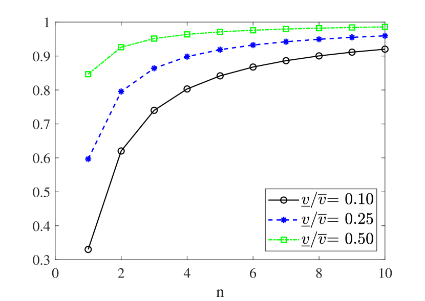
(a) $\mathcal{R}_{n}/\mathcal{R}_{\infty}$ for $n=1,\dots,10$, with $\frac{\underline{v}}{\bar{v}}=0.1,0.25,0.5$ under Support Ambiguity Set

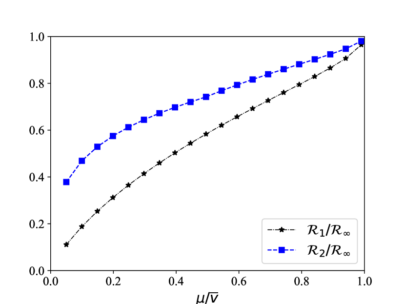
(b) $\mathcal{R}_{n}/\mathcal{R}_{\infty}$ for $n=1,2$ under Mean Ambiguity Set

We then consider the mean ambiguity set, where the mean of the buyer’s valuation is greater than or equal to $\mu$ and the upper bound of the valuation is $\bar{v}$. Based on the finite linear programming formulation we provide, we characterize the optimal pricing mechanism under 1-level pricing and 2-level pricing. In Section 4.1, we show that for 1-level pricing, the optimal posted price is $\bar{v}-\sqrt{\bar{v}^{2}-\mu\bar{v}}$ and the optimal competitive ratio is $1-\sqrt{1-\mu/\bar{v}}$. For any posted price, nature’s strategy can be a single-point distribution at $\bar{v}$ or a two-point distribution at both $\bar{v}$ and a valuation slightly lower than the posted price. Hence, incorporating a second price level between $v_{1}$ and $\bar{v}$ can significantly improve the competitive ratio. In Section 4.2, we provide the closed-form characterization for the optimal 2-level pricing mechanism and the optimal competitive ratio. For the 2-level pricing, the lower price should be equal to the optimal posted price in 1-level pricing, and the higher price should be greater than $\mu$ when $\mu$ is small and less than $\mu$ when $\mu$ is large. Figure 1(b) depicts $\mathcal{R}_{1}/\mathcal{R}_{\infty}$ and $\mathcal{R}_{2}/\mathcal{R}_{\infty}$ with the ratio between the valuation mean $\mu$ and upper bound $\bar{v}$ ranging from 0 to 1, where $\mathcal{R}_{1},\mathcal{R}_{2},\mathcal{R}_{\infty}$ stand for the competitive ratios achieved by 1-level, 2-level, and $\infty$-level pricing models, respectively. It shows that under a moderate mean, the $2$-level pricing mechanism can close the gap between the competitive ratios obtained by the $\infty$-level pricing and $1$-level pricing significantly.

In addition, we apply our framework to solve the optimal robust selling mechanisms for $n=1,2,\infty$ under the quantile ambiguity set. The quantile ambiguity set suggests that, given the historical sales data, the seller estimates a lower bound of $\xi$ for the probability that the buyer’s valuation equals or exceeds $\omega$. Based on our finite linear programming formulation, we characterize the optimal pricing mechanisms and the corresponding competitive ratios under 1-level pricing, 2-level pricing, and $\infty$-level pricing (optimal robust mechanism). In Section 5, we show that the optimal posted price is $\omega$ and the optimal competitive ratio is $\min\{\xi,\frac{\omega}{\bar{v}}\}$ for 1-level pricing. Besides, we provide a closed-form characterization of the optimal mechanism in 2-level pricing. The corresponding competitive ratio achieved by 2-level pricing indicates a significant improvement over the 1-level pricing. In addition, we illuminate the optimal $\infty$-level pricing, i.e., optimal robust mechanism without menu-size constraints, together with the optimal competitive ratio. Figure 2 illustrates the comparison of the competitive ratios obtained by 1-level and 2-level pricing models to that of the $\infty$-level model under varying quantile information. Our results exhibit that the gap between the competitive ratios based on $\infty$-level pricing and that based on 1-level pricing can be significantly reduced by incorporating the 2-level pricing model.

Figure 2: $\mathcal{R}_{1}/\mathcal{R}_{\infty}$ and $\mathcal{R}_{2}/\mathcal{R}_{\infty}$ Under the Quantile Ambiguity Set

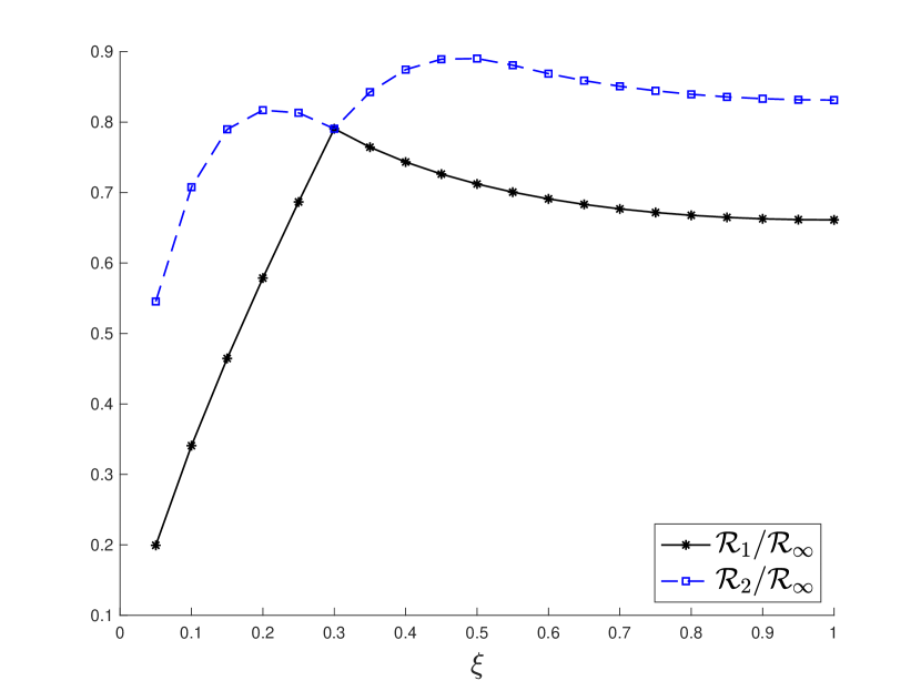
(a) $\omega/\bar{v}=0.3$

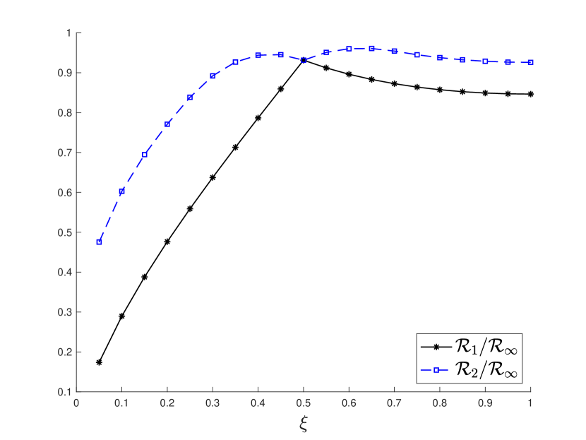
(b) $\omega/\bar{v}=0.5$

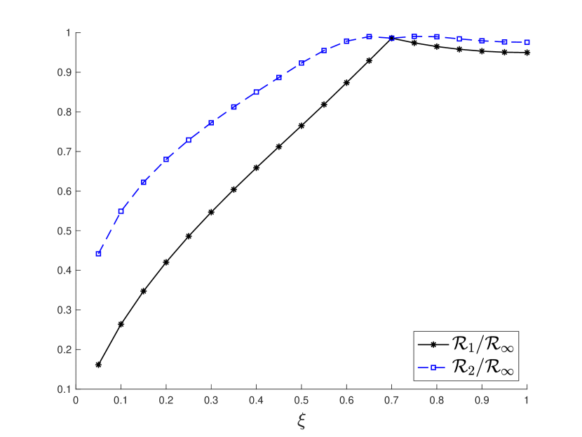
(c) $\omega/\bar{v}=0.7$

Finally, we also investigate the empirical performance of the $n$-level pricing for $n=1,2,\infty$ in different distributions. The experiments demonstrate that the performance of 2-level pricing is close to that of the $\infty$-level pricing under most circumstances, and it also outperforms the $\infty$-level pricing in certain scenarios. Essentially, our framework enables the analysis of $n$-level pricing problems under a broad class of ambiguity sets, which leads to closed-form competitive ratios for 1-level, 2-level and $\infty$-level pricing problems. Our findings highlight the substantial effectiveness of 2-level pricing mechanisms across different ambiguity sets, and our research could serve as a stepping stone for future research to better understand the value associated with simple menus in robust mechanism design.

1.1 Related Literature

Our work belongs to the literature on robust mechanism design. One of the most important and widely studied objectives is to maximize worst-case revenue based on different ambiguity sets. Bergemann and Schlag (2011) study the single-item and single-buyer problem assuming the buyer’s actual distribution is within a small neighborhood under the Prohorov metric of a given benchmark distribution. Carrasco et al. (2018) investigate the optimal robust selling mechanism under moments information, and provide closed-form optimal mechanism under mean-variance and mean-support ambiguity sets. They show that the worst-case revenue achieved by the optimal mechanism is higher than that achieved by the optimal deterministic pricing. Pınar and Kızılkale (2017) study the maximin revenue model with moment information under discrete support. They also discuss the implementation challenges of the optimal mechanism compared to the simple deterministic pricing. Li et al. (2019) solve the optimal robust mechanism under the maximin-revenue model in an ambiguity set based on the Wasserstein metric for both single-buyer and multi-buyer problems. Chen et al. (2021) provide a novel geometric approach based on strong duality between the robust mechanism design problem and the minimax pricing problem, and recover the results in a broad class of ambiguity sets, including the moments ambiguity set and Wasserstein ambiguity set, among others. Beyond the maximin revenue criterion, Bergemann and Schlag (2008) and Eren and Maglaras (2010) study the robust mechanism design problem with support information under the minimax absolute regret criterion and maximin competitive ratio criterion, respectively. Caldentey et al. (2017) study the dynamic pricing with support ambiguity set under the minimax absolute regret criterion. Wang et al. (2020) study the maximin ratio criterion under the moments information. In the multi-item setting, the robust mechanism is investigated under support ambiguity set (Bandi and Bertsimas 2014), marginal distributions (Carroll 2017, Gravin and Lu 2018), and partial information on the marginal distributions (Koçyiğit et al. 2020, 2022). In the auction setting, the robust mechanism is studied under partial information on the joint distributions from the bidders (Azar and Micali 2013, Azar et al. 2013, Fu et al. 2019, Allouah and Besbes 2020)

Our work is also closely related to the literature on robust deterministic pricing. Chen et al. (2022) study robust deterministic pricing under the mean and variance ambiguity set, both for single-product and for multi-product problems. Chen et al. (2023) study a robust pricing model based on asymmetric information of the customers’ valuation distribution including mean, variance, and semivariance. Cohen et al. (2021) study the robust pricing problem without knowing the form of the demand curve. They show that posting price assuming the demand function is linear has good performance guarantees under different classes of demand curves. Elmachtoub et al. (2021) provide the upper and lower bounds of the competitive ratio between the optimal deterministic price and idealized personalized pricing. Allouah et al. (2023) characterize the optimal robust pricing and screening with quantile information under regular and monotone hazard-rate distributions. Another important stream of this literature has studied pricing problems with samples drawn from the valuation distribution (Cole and Roughgarden 2014, Dhangwatnotai et al. 2015, Fu et al. 2015, Gonczarowski and Nisan 2017, Huang et al. 2018, Allouah et al. 2022, Guo et al. 2019, Hu et al. 2021), which investigates the sample complexity to achieve a target competitive ratio.

Since the seminal work Myerson (1981) established that simple auctions are optimal when the seller knows the exact valuation distributions of buyers, there has been a wealth of literature examining the optimal mechanism for multi-item, multi-bidder problems. These problems prove challenging and the optimal mechanism may have an infinite number of menu options. This complexity has motivated a substantial and invaluable stream of research that explores the performance of simple mechanisms, such as bundling, separation, mechanisms with a limited number of menu options, and auctions with randomized reserve prices, among others (Hartline and Roughgarden 2009, Hart et al. 2013, Wang and Tang 2014, Babaioff et al. 2017, Cai and Zhao 2017, Hart and Nisan 2017, 2019, Babaioff et al. 2020, Eden et al. 2021, Feng et al. 2023). Researchers have also identified specific conditions on valuation distributions under which the optimal mechanisms are found within a class of simple mechanisms. The findings from these studies have been remarkable, offering insightful implications for optimal mechanism design problems when the exact valuation distribution is known. However, the methodology applied in optimal mechanism design, given a valuation distribution, is substantially different from our approach in the robust mechanism design setting. In this work, we endeavor to solve the robust selling mechanism with a limited menu size, which could strike a favorable balance between superior theoretical performance inherent to robust mechanism design and feasible practical implementation provided by robust deterministic pricing.

The power of sparse solutions or simple policy structures is also studied in various domains. For example, Jordan and Graves (1995), Bassamboo et al. (2010), Chou et al. (2010, 2011), Simchi-Levi and Wei (2012, 2015), Chou et al. (2014), Wang and Zhang (2015), Bidkhori et al. (2016), Shi et al. (2019), Wang et al. (2022, 2023) investigate the effectiveness of the long chain (two-chain) structure compared to the fully flexible structure in process flexibility design for supply chain network. Bassamboo et al. (2012), Tsitsiklis and Xu (2013, 2017) study the efficiency of sparse structures in balancing delay cost or capacity region and the cost generated in flexibility design for queueing systems. Chen and Dong (2021) shows that compared with the shortest-remaining-processing-time-first policy, the two-class priority rule is also near-optimal. Balseiro et al. (2023) shows it is effective to switch between two prices based on the inventory level in reusable resource allocation. In our work, we shed light on the effectiveness of a menu with two options in the robust selling mechanisms, which is easy to implement for practitioners.

2 $n$-Level Robust Pricing Problem

We consider a monopolist selling a product to a group of homogeneous buyers whose valuation of the product is unknown to the seller. The seller knows that the buyer’s valuation $v$ is within $[0,\bar{v}]$, but does not know the exact valuation distribution. By the revelation principle (Myerson 1981), the seller can restrict his attention to a direct mechanism $(q,t)$ without loss of revenue, where $q:[0,\bar{v}]\rightarrow[0,1]$ denotes an allocation rule, and $t:[0,\bar{v}]\rightarrow\mathbb{R}$ denotes a transfer or payment rule. The feasible set of mechanisms satisfies two sets of constraints as follows: individual rationality (IR) constraints, ensuring that the buyer is incentivized to participate in the seller’s mechanism, and the incentive-compatibility (IC) constraints, ensuring that the buyer is deterred from misreporting her valuation. Hence, the feasible set of mechanisms can be represented as follows, where the constraint $t(0)=0$ is applied because it is optimal to set the payment to 0 for a buyer with a valuation of 0, and the continuity constraint is technical and without loss of revenue.

$$\left\{(q,t):[0,\bar{v}]\rightarrow[0,1]\times\mathbb{R}\ \left|\ \begin{matrix}vq(v)-t(v)\geq 0,\ \forall v\in[\underline{v},\bar{v}]\\ vq(v)-t(v)\geq vq(v^{\prime})-t(v^{\prime}),\ \forall v,v^{\prime}\in[\underline{v},\bar{v}]\\ t(0)=0\mbox{ and }q(\cdot)\mbox{ is right-continuous}\end{matrix}\right.\right\}.$$

Accordingly, for a buyer with a valuation $v$, the seller allocates the product with probability $q(v)$ and requests a payment of $t(v)$. It is shown in mechanism design literature that a direct mechanism is incentive compatible if and only if the allocation rule $q(v)$ is increasing in $v$ and the payment rule is specified by $t(v)=vq(v)-\int_{0}^{v}q(u)du$ (Myerson 1981). This mechanism can be represented by showing a menu of lotteries to the buyer. Each lottery, indexed by $v$, consists of an allocation probability of $q(v)$ and a payment $t(v)$. At the same time, this mechanism is also payoff-equivalent to a randomized pricing mechanism with a price density function of $x(\cdot)$, where the allocation rule $q(\cdot)$ serves as the cumulative price distribution, i.e., $q(v)=\int_{0}^{v}x(u)du$. Formally, the set of feasible mechanisms can be represented by the set of all price density functions defined on $[0,\bar{v}]$,

$$\mathcal{X}:=\left\{\mathbf{x}:[0,\bar{v}]\rightarrow\mathbb{R}^{+}\,\Big{|}\,\int_{0}^{\bar{v}}x(u)du=1\right\}$$

or equivalently, by the set of allocation rules $\mathcal{Q}:=\big{\{}\mathbf{q}:[0,\bar{v}]\rightarrow[0,1]\,\big{|}\,q(v)\text{ is increasing in }v\text{ and }q(\bar{v})=1\big{\}}$. Most of the optimal robust mechanisms derived in the literature involve offering a menu of infinite lotteries or randomizing over prices in a continuous interval, which may bring implementation challenges in practice. In this work, we investigate how the complexity, characterized by the menu size or the number of prices that the seller randomizes over, affects the effectiveness of the robust mechanism. In particular, we focus on the set of feasible mechanisms that offer a finite menu of lotteries or equivalently, randomize over a finite number of prices. We denote $n$-level pricing mechanisms as the set of mechanisms that randomize over no more than $n$ distinct prices, represented by $\mathcal{X}_{n}$.

$$\mathcal{X}_{n}:=\{\mathbf{x}:[0,\bar{v}]\rightarrow\mathbb{R}_{+}\mid\exists\,v_{1}\leq\dots\leq v_{n}\in[0,\bar{v}],\mbox{s.t.}\,\sum_{i=1}^{n}x(v_{i})=1,\mbox{and }\,x(v)=0,\forall v\neq v_{i},i=1,\dots,n\}$$

Here $n=1,2\dots$, and the definition above implies that $\mathcal{X}_{n}\subseteq\mathcal{X}_{\hat{n}}$, for any $\hat{n}\geq n$. Each element $\mathbf{x}\in\mathcal{X}_{n}$ denotes a price density function, which defines a randomized pricing selling mechanism.

For any given buyer’s valuation distribution $\mathbb{F}$, the expected revenue achieved by a mechanism $\mathbf{x}\in\mathcal{X}_{n}$ is characterized as $\mathrm{Rev}(\mathbf{x},\mathbb{F})=\int_{0}^{\bar{v}}(\int_{0}^{v}x(u)u\,du)\,d\mathbb{F}(v)$. This is because, for a buyer with a valuation $v$, the expected payment that she makes is $t(v)=\int_{0}^{v}x(u)u\,du$. Hence, the expected revenue that the seller obtains is $\int_{0}^{\bar{v}}t(v)d\mathbb{F}(v)=\int_{0}^{\bar{v}}(\int_{0}^{v}x(u)u\,du)\,d\mathbb{F}(v)$. Upon determining the mechanism, the seller does not know the buyer’s valuation distribution $\mathbb{F}$ but knows only that $\mathbb{F}\in\mathcal{F}$ for some convex ambiguity set $\mathcal{F}.$ In order to evaluate the effectiveness of a robust mechanism, we adopt the optimal revenue achieved by a clairvoyant who knows the buyer’s valuation distribution as the benchmark. Given any valuation distribution $\mathbb{F}$, the optimal mechanism is to set a posted price at $\arg\max_{p\geq 0}p(1-\mathbb{F}(p-))$. We denote the revenue achieved by this benchmark as $\mathrm{Rev}(\mathsf{OPT},\mathbb{F})=\max_{p\geq 0}\ p(1-\mathbb{F}(p-)).$ Thus, the performance of a mechanism $\mathbf{x}\in\mathcal{X}_{n}$ is evaluated by the competitive ratio, which is the worst-case ratio between the revenue obtained by mechanism $\mathbf{x}$ and that obtained by the optimal mechanism given the valuation distribution:

$$\mathrm{CR}(\mathbf{x})=\inf_{\mathbb{F}\in\mathcal{F}}\frac{\mathrm{Rev}(\mathbf{x},\mathbb{F})}{\mathrm{Rev}(\mathsf{OPT},\mathbb{F})}=\inf_{\mathbb{F}\in\mathcal{F}}\frac{\int_{0}^{\bar{v}}(\int_{0}^{v}x(u)u\,du)\,d\mathbb{F}(v)}{\max_{p\in[0,\bar{v}]}\ p(1-\mathbb{F}(p-))},$$

For any finite menu size $n$, we aim to construct a mechanism that achieves a desirable competitive ratio among all distributions within the ambiguity set $\mathcal{F}$. We formulate this robust $n$-level pricing problem as follows:

$$\sup_{\mathbf{x}\in\mathcal{X}_{n}}\mathrm{CR}(\mathbf{x})=\sup_{\mathbf{x}\in\mathcal{X}_{n}}\inf_{\mathbb{F}\in\mathcal{F}}\frac{\int_{0}^{\bar{v}}(\int_{0}^{v}x(u)u\,du)\,d\mathbb{F}(v)}{\max_{p\in[0,\bar{v}]}\ p(1-\mathbb{F}(p-))}$$ (1)

Problem (1) can be formulated as a zero-sum game between the seller and nature. For any selling mechanism that the seller adopts, the nature will adversarially choose the worst-case distribution $\mathbb{F}$ from the ambiguity set $\mathcal{F}$ and the corresponding optimal posted price $p\in[0,\bar{v}]$ such that the competitive ratio is minimized. The ambiguity set we consider takes the following form:

$$\mathcal{F}=\left\{\mathbb{F}\in\mathcal{P}([0,\bar{v}]):\,\int_{v\in[0,\bar{v}]}\phi_{k}(v)\,d\mathbb{F}(v)\geq 0,\ \forall k=1,2\ldots,K.\right\}.$$ (2)

where $K$ is a given number, $\phi_{k}$ is a predetermined function of $v$, and $\mathcal{P}([0,\bar{v}])$ represents the set of all probability measures on $[0,\bar{v}]$. In the following illustration, we will demonstrate that (2) encompasses several ambiguity sets commonly found in the literature or in practice.

1. Support ambiguity set: If there is only one constraint in (2) that $\phi(v)=\mathbbm{1}[v\geq\underline{v}]-1$, the resulting ambiguity set can be represented as $\mathcal{F}=\left\{\mathbb{F}\in\mathcal{P}([0,\bar{v}]):\,\int_{v=0}^{\bar{v}}\mathbbm{1}[v\geq\underline{v}]\,d\mathbb{F}(v)\geq 1\right\}$. This corresponds to the support ambiguity set, focusing on distributions where the buyer’s valuation is certain to fall between $\underline{v}$ and $\bar{v}$.

2. Moments ambiguity set: In the case where the functions $\phi_{k}(v)=v^{l}-\mu_{l}$ for certain $k$’s, while $\phi_{k}(v)=\mu_{l}-v^{l}$ for other $k$’s, the ambiguity set (2) represents the moments ambiguity set. In this case, $\mathcal{F}=\left\{\mathbb{F}\in\mathcal{P}([0,\bar{v}]):\,\int_{v\in[0,\bar{v}]}v^{k}\,d\mathbb{F}(v)=\mu_{k},\ \forall k=1,2\ldots,K.\right\}$. This ambiguity set allows us to focus on distributions where specific moments of the buyer’s valuation match the estimated values. Note that some constraints in this set can be modified to inequalities by removing one side of the constraints. For more detailed discussions on this ambiguity set, please refer to Carrasco et al. (2018), Wang et al. (2020).

3. Quantile ambiguity set: If we define $\phi_{k}(v)=\mathbbm{1}[v\geq\omega_{k}]-\xi_{k}$ where $\omega_{k}\in[0,\bar{v}]$, the ambiguity set (2) corresponds to the quantile ambiguity set, represented as $\mathcal{F}=\left\{\mathbb{F}\in\mathcal{P}([0,\bar{v}]):\mathbb{P}[v\geq\omega_{k}]\geq\xi_{k},\ \forall k=1,2,\dots,K\right\}$. In this ambiguity set, the focus is on distributions where the purchasing probability for a posted price $\omega_{k}$ is greater than or equal to $\xi_{k}$ for all $k=1,\dots,K$. In practice, the seller can estimate these purchasing probabilities $\xi_{k}$ corresponding to some posted price $\omega_{k}$ based on historical sales data. Please refer to Allouah et al. (2023) for more discussions on this ambiguity set.

4. Multi-Segment ambiguity set: If we define $\phi_{k}(v)=\mathbbm{1}[v\in I_{k}]-\xi_{k}$, for $k=1,\dots,K$, where $I_{k}=[a_{1}^{k},b_{1}^{k}]\cup[a_{2}^{k},b_{2}^{k}]\cup\dots\cup[a_{l_{k}}^{k},b_{l_{k}}^{k}]$, where $l_{k}=1,2,\dots$, the ambiguity set in (2) corresponds to what we call a multi-segment ambiguity set. In this scenario, the seller assumes a lower bound $\xi_{k}$ on the probability that a buyer’s valuation falls within the union of specific intervals, denoted by $I_{k}$. Moreover, by incorporating multiple constraints, the seller can assert various lower bounds corresponding to distinct market segments, which could potentially overlap. For instance, if $\phi_{k}(v)=\mathbbm{1}[v\in[a_{k},b_{k}]]-\xi_{k}$ for all $k=1,\dots,K$, the seller posits that the probability of the buyer’s valuation falling within the interval $[a_{k},b_{k}]$ is at least $\xi_{k}$, for every $k=1,\dots,K$, where intervals $[a_{k},b_{k}]$ can be overlapping with each other.

5. Segmented-Statistics ambiguity Set: Suppose $\phi_{k}(v)=\mathbbm{1}[v\in I_{k}]\cdot(v^{l}-\mu_{kl})$, where $I_{k}\subseteq[0,\bar{v}]$ is defined as in the previous example. In this case, the ambiguity set suggests that the $l$th moment of the valuation within the subset $I_{k}$ is at least $\mu_{kl}$. This type of ambiguity set accounts for situations where the seller has only partial statistical information about a subset of the buyers. For instance, suppose the seller collected data only for buyers whose valuation exceeds a certain threshold, say $\hat{v}$, then estimated the mean and variance for this market segment. This ambiguity set would allow the seller to make pricing decisions even with limited and segment-specific information about buyer valuations.

Building on the ambiguity set defined in (2), we are able to transform the maximin ratio problem in (1) into a maximization problem as per (3) in Proposition 2.1. This transformation results in a problem formulation that is subject only to linear constraints, except for the constraints defined within $\mathcal{X}_{n}$.

Proposition 2.1

The $n$-level robust pricing Problem (1) is equivalent to Problem (3), where the optimal solution $r$ is the optimal competitive ratio, and $\mathbf{x}$ is the corresponding optimal price density function.

$$\sup\limits_{\boldsymbol{\lambda}\in\mathbb{R}^{K\times[0,\bar{v}]}_{+},\ \mathbf{x}\in\mathcal{X}_{n},\ r\in\mathbb{R}^{+}} r$$ (3)

$$\mathrm{s.t.} \sum_{k=1}^{K}\phi_{k}(v)\lambda_{k}(p)\leq\int_{0}^{v}x(u)u\,du\quad\forall p\in[0,\bar{v}],\ \forall v\in[0,p)$$

$$r\cdot p+\sum_{k=1}^{K}\phi_{k}(v)\lambda_{k}(p)\leq\int_{0}^{v}x(u)u\,du\quad\forall p\in[0,\bar{v}],\ \forall v\in[p,\bar{v}]$$

Proposition 2.1 has simplified the max-min Problem (1) to a maximization problem with linear constraints. However, the problem is still challenging, due to the infinite-dimensional decision variables and the infinite number of constraints. Moreover, since the feasible set of randomized pricing mechanisms defined in $\mathcal{X}_{n}$ is non-convex, Problem (3) is still hard to solve in general. Next, we first fix the set of possible price levels $\mathcal{V}=\{v_{1},\dots,v_{n}\}$ and simplify (3) by introducing the following assumption. In the ambiguity set definition given by (2), each $\phi_{k}(v)$ is a piecewise continuous function and is nondecreasing in $v$ within each segment. We will now show that most ambiguity sets that we discussed previously— including the support ambiguity set, mean ambiguity set, quantile ambiguity set, multi-segment ambiguity set, and segmented-mean ambiguity set—satisfy Proposition 2.1.

1. Support ambiguity set: Here, $\phi(v)=\mathbbm{1}[v\geq\underline{v}]-1$. This is a step function, which is piecewise continuous, thereby satisfying Assumption 2.1.

2. Mean ambiguity set: In this case, $\phi(v)=v-\mu$, which is a linear function of $v$, satisfying Proposition 2.1. The ambiguity set assumes that $\mathbb{E}[v]\geq\mu$.

3. Quantile ambiguity set: Here $\phi_{k}(v)=\mathbbm{1}[v\geq\omega_{k}]-\xi_{k}$, which is a step function, satisfying Proposition 2.1.

4. Multi-Segment ambiguity set: Here $\phi_{k}(v)=\mathbbm{1}[v\in I_{k}]-\xi_{k}$, for $k=1,\dots,K$, which is a step function with value $1-\xi_{k}$ within interval $I_{k}$ and $-\xi_{k}$ outside $I_{k}$, thereby satisfying Proposition 2.1.

5. Segmented-Mean Ambiguity Set: In this case, $\phi_{k}(v)=\mathbbm{1}[v\in I_{k}]\cdot(v-\mu_{k})$, which is a piecewise linear function of $v$, satisfying Proposition 2.1. Here one assumes that the mean of the valuation in market segment $I_{k}$ is at least $\mu_{k}$.

The above illustrations underline the general applicability of Proposition 2.1. Nonetheless, we also admit the limitations of Proposition 2.1. For instance, the mean-variance ambiguity set, which is widely discussed, does not satisfy Proposition 2.1. The introduction of Proposition 2.1 is for the tractability of the $n$-level pricing problem. Though Proposition 2.1 does not cover some important ambiguity sets, we believe the main insights we present in the paper also hold for more general ambiguity sets.

In the following, we are going to further simplify and analyze the robust pricing problem in (3) based on Proposition 2.1. According to Proposition 2.1, each $\phi_{k}$ is piecewise continuous for $k=1,\dots,K$, so there will be a finite number of breakpoints for each $\phi_{k}(\cdot)$. Consequently, the aggregate of all breakpoints in $\phi_{k}(\cdot)$ for all $k=1,\dots,K$ will also be finite. We denote the set of all breakpoints for $\phi_{k}(\cdot)$’s as $\mathcal{B}=\{b_{1},\dots,b_{m}\}$, where $0<b_{1}<\dots<b_{m}<\bar{v}$. Consider any set of price levels $\mathcal{V}=\{v_{1},\dots,v_{n}\}$. We arrange all the valuations in $\mathcal{B}$ and $\mathcal{V}$ in ascending order, such that $u_{1}\leq u_{2}\leq\dots\leq u_{m+n}$, where $u_{j}\in\mathcal{V}\cup\mathcal{B}$ for all $j=1,\dots,m+n$. For notational simplicity, we represent $u_{n+m+1}=\bar{v}$. In Theorem 2.2, we establish a finite linear programming formulation for the $n$-level pricing problem with fixed price levels. Hereafter, when the values of price levels: $v_{1},\dots,v_{n}$ are specified without ambiguity, with a slight abuse of notation, we denote $\mathbf{x}=[x_{1},x_{2},\dots,x_{n}]$ as the probability associated with each price level. For further notational clarity, we define $\underline{\phi}_{k,j}=\lim_{v\rightarrow u_{j}-}\phi_{k}(v)$ for $k=1,\dots,K,j=1,\dots,n+m+1$, and we denote $S_{j}=\{l=1,\dots,n\mid v_{l}<u_{j}\}$ for $j=1,\dots,n+m+1$.

Theorem 2.2 (Finite-LP)

Under Proposition 2.1, for any given price level set $\mathcal{V}$ and breakpoint set $\mathcal{B}$, the seller’s $n$-level pricing problem is equivalent to the following finite linear programming problem, where $x_{i}$ is the probability that the seller sets price $v_{i}$ for $i=1,\dots,n$, and $r$ is the corresponding competitive ratio.

$$\sup\limits_{\begin{subarray}{c}\boldsymbol{\lambda}\in\mathbb{R}^{K\times(m+n+1)}_{+}\\ \mathbf{x}\in\mathbb{R}_{+}^{n},r\in\mathbb{R}^{+}\end{subarray}} r$$ (4)

$$\mathrm{s.t.} \sum_{k=1}^{K}\underline{\phi}_{k,j}\lambda_{k,i}\leq\sum_{l\in S_{j}}v_{l}x_{l},\ \forall\ i\in[n+m+1],\,j\in[i-1]$$

$$r\cdot u_{i}+\sum_{k=1}^{K}\underline{\phi}_{k,j}\lambda_{k,i}\leq\sum_{l\in S_{j}}v_{l}x_{l},\ \forall\ i\in[n+m+1],\,j=i,\dots,n+m+1$$

$$\sum_{i=1}^{n}x_{i}=1$$

Theorem 2.2 reduces the number of variables and constraints in (3) to finite, which simplifies the analysis significantly. In light of Theorem 2.2, we are able to characterize the performance ratio of robust mechanisms with different price levels (or menu sizes) under some important ambiguity sets satisfying Proposition 2.1. In the remaining sections, we will develop tractable simplifications of (4) based on different specifications on the ambiguity sets.

3 Support Ambiguity Set

In this section, we assume that the seller knows there is a lower bound of the buyer’s valuation, denoted as $\underline{v}$. Hence, the ambiguity set is specified by $\mathcal{F}=\left\{\mathbb{F}\in\mathcal{P}([0,\bar{v}]):\,\int_{\underline{v}}^{\bar{v}}\,d\mathbb{F}(v)\geq 1\right\}.$ In this specification, there is only one constraint in $\mathcal{F}$, which is $\phi(v)=\mathbbm{1}[v\geq\underline{v}]-1$. For ease of reference, we do not include the subscript $k=1$. Since the buyer’s valuation cannot fall below $\underline{v}$, it is suboptimal to post a price lower than $\underline{v}$, so we can focus on the prices equal to or greater than $\underline{v}$. Within the domain $v\geq\underline{v}$, the term $\phi(v)$ is consistently valued at $1-1=0$. As a result, the coefficients for $\boldsymbol{\lambda}$ are zero in Problem (4), allowing us to eliminate the decision variables $\boldsymbol{\lambda}$. Given price level set $\mathcal{V}=\{v_{1},\dots,v_{n}\}$, Problem (4) is specified as

$$\displaystyle\sup\limits_{\mathbf{x}\in\mathbb{R}_{+}^{n},r\in\mathbb{R}^{+}} \,r$$ (5)

$$\mathrm{s.t.}\quad r\cdot v_{i}\leq\sum_{j=1}^{i-1}x_{j}\cdot v_{j}\quad\forall i=2,\dots,n+1.$$ (5a)

$$r\cdot v_{1}\leq x_{1}\cdot v_{1}\cdot\mathbbm{1}[v_{1}=\underline{v}]$$ (5b)

$$\sum_{i=1}^{n}x_{i}=1$$ (5c)

where $v_{n+1}=\bar{v}$ for notational simplicity. From constraint (5b), we observe that if $v_{1}>\underline{v}$, it would result in a non-positive competitive ratio, i.e., $r\leq 0$. Thus, for any randomized pricing mechanism, we must have $v_{1}=\underline{v}$. In Figure 3(a), we offer a graphical representation of the constraints in Problem (5) to provide an intuitive understanding. As depicted in Figure 3(a), given any feasible $v_{1},\dots,v_{n}$ and $x_{1},\dots,x_{n}$, the optimal feasible $r^{*}$ represents the largest possible slope of the function $r\cdot v$ which remains below the step function $\sum_{j=1}^{i}x_{j}\cdot v_{j}$, where $i=\max\{i^{\prime}:v_{i^{\prime}}\leq v\}$. In order to maximize $r$, one can adjust $\mathbf{x}$ such that the breakpoints of the step function align with the line $r\cdot v$, as illustrated in Figure 3(b). Therefore, for any feasible price level set $\mathcal{V}=\{v_{1},\dots,v_{n}\}$, where $v_{1}=\underline{v}$, it is possible to enhance $r$ by manipulating $\mathbf{x}$ to satisfy constraints (5a) and (5b) as equalities. Hence, the optimal $x_{1},\dots,x_{n}$ and $r$ can be solved by $r=\frac{\sum_{j=1}^{i}x_{j}\cdot v_{j}}{v_{i+1}},\,\forall\ i=1,\dots,n.$

Figure 3: Payment Function $\sum_{j=1}^{i}x_{j}v_{j}$ for $x\in[v_{i},v_{i+1})$ together with $r\cdot v$

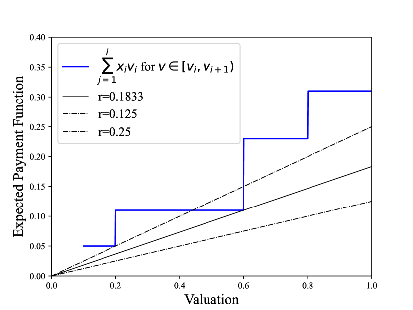
(a) Arbitrary $\mathbf{x}$ for fixed $\mathcal{V}$

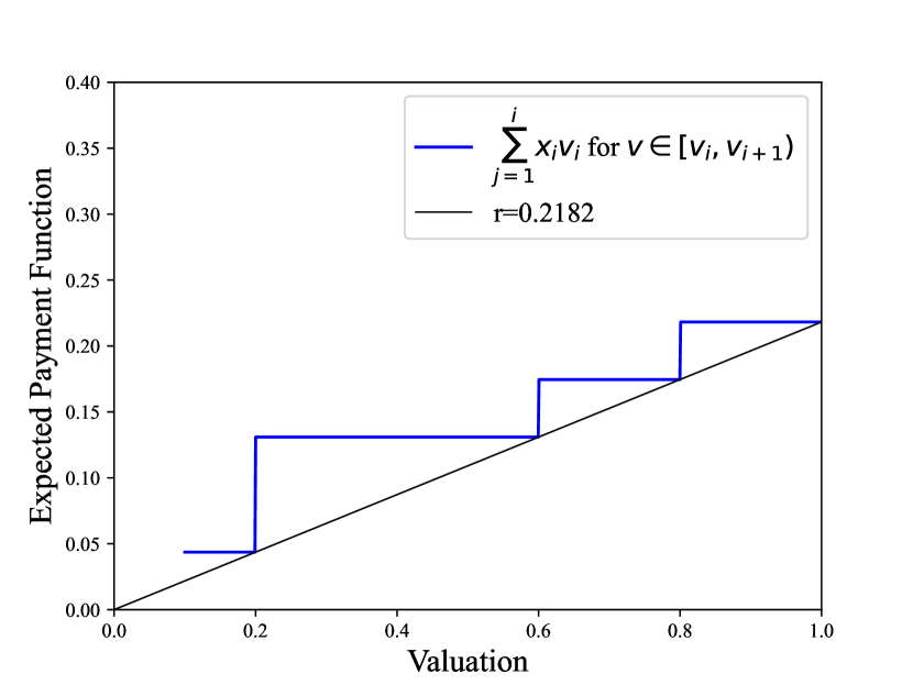
(b) Optimal $\mathbf{x}$ for Fixed $\mathcal{V}$

In Lemma 3.1, we formalize the optimal competitive ratio $r$ and the corresponding pricing probability $\mathbf{x}$ for a given price level set $\mathcal{V}$.

Lemma 3.1

For any given price level set $\mathcal{V}=\{v_{1},v_{2}\ \dots,\ v_{n}\}$, where $v_{1}=\underline{v}$, the optimal competitive ratio is $r=\big{(}\frac{v_{2}}{v_{1}}+\sum_{i=2}^{n}\frac{v_{i+1}-v_{i}}{v_{i}}\big{)}^{-1}$, and the optimal pricing probability is determined by $x_{1}=r\cdot\frac{v_{2}}{\underline{v}},\,x_{i}=r\cdot\frac{v_{i+1}-v_{i}}{v_{i}},\,\forall\ i=2,\dots,n$.

Lemma 3.1 can be intuitively explained as follows. For any given price levels $\mathcal{V}=\{v_{1},\dots,v_{n}\}$ and seller’s pricing policy $x_{1},\dots,x_{n}$, the worst-case distribution that nature selects is to search from valuations that approach $v_{i}$ from the left for each $i=2,\dots,\bar{v}$, and then find the valuation that can minimize the ratio between the seller’s revenue and its true valuation, i.e., $\frac{\sum_{j=1}^{i-1}v_{j}x_{j}}{v_{i}-}$, for $i=2,\dots,n$. In order to hedge against this adversary, the seller adopts pricing probabilities $x_{1},\dots,x_{n}$ such that the ratio of the expected payment at each $v_{i}-$ relative to its valuation $v_{i}-$, remains equal across all $v_{i}-,\ \forall i=2,\dots,n$. Next, based on the optimal competitive ratio and the corresponding pricing probability $\mathbf{x}$ assigned to each price level defined in Lemma 3.1, we proceed to optimize the selection of pricing levels $\mathcal{V}$. In Proposition 3.2, we characterize the optimal $n$-level pricing mechanism and the corresponding competitive ratio for each $n$. As illustrated in Proposition 3.2, the optimal price levels for any $n$-level pricing scheme form a geometric sequence, and the optimal pricing probabilities assigned are equal for each price level except the first price level at $\underline{v}$.

Proposition 3.2

Suppose the buyer’s valuation is within support $[\underline{v},\bar{v}]$. Then the optimal competitive ratio the seller achieves by adopting an $n$-level randomized pricing strategy is $\mathcal{R}_{n}=\big{(}n(\bar{v}/\underline{v})^{1/n}-(n-1)\big{)}^{-1}$. Besides, the optimal price levels form a geometric sequence defined as: $v_{i}=\underline{v}^{\frac{n+1-i}{n}}\cdot\bar{v}^{\frac{i-1}{n}},\quad i=1,\dots,n.$ The optimal pricing probabilities assigned to each price level are equal except for the first price level at $\underline{v}$, i.e. $x_{1}=(\bar{v}/\underline{v})^{1/n}\cdot\mathcal{R}_{n},\quad x_{i}=((\bar{v}/\underline{v})^{1/n}-1)\cdot\mathcal{R}_{n},\quad i=2,\dots,n.$

As the number of price levels increases, the competitive ratio approaches that of the optimal robust mechanism facilitated by a continuous randomized pricing scheme:

$$\lim_{n\rightarrow\infty}\mathcal{R}_{n}=\lim_{n\rightarrow\infty}\big{(}n(\bar{v}/\underline{v})^{1/n}-(n-1)\big{)}^{-1}=\lim_{n\rightarrow\infty}\big{(}n((\bar{v}/\underline{v})^{1/n}-1)+1\big{)}^{-1}=\big{(}\ln(\bar{v}/\underline{v})+1\big{)}^{-1}$$

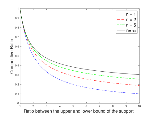
Figure 4: Competitive Ratio of $n$-Level Pricing for n=1, 2, 5, and infinity

In Figure 4, we compare the competitive ratio for different price levels ranging from 1, 2, 5, 100, and infinity under different ratios between the upper and lower bounds of the buyer’s valuation support. It is shown that the competitive ratio decreases with the ratio between the upper and lower bounds, and the decreasing rate of the 1-level pricing scheme is steeper compared to other mechanisms with higher price levels. Figure 4 emphasizes the substantial improvement in the competitive ratio when evolving from a 1-level pricing scheme to a 2-level randomized pricing scheme. Specifically, by merely introducing one additional price level, the discrepancy between the competitive ratio of the 1-level pricing scheme and that of the optimal robust mechanism is cut approximately in half. Furthermore, a 5-level randomized pricing scheme yields a competitive ratio that closely approximates the optimal competitive ratio achievable with continuous randomized pricing. This suggests that a finite, and notably modest, set of price levels can capture a substantial proportion of the benefit associated with continuous randomized pricing. This observation provides practical implications for sellers who are concerned about the complexity of menu sizes in real-world market conditions, and it offers a clear path for sellers to balance profitability and operational practicality.

4 Mean Ambiguity Set

Suppose the seller knows that the buyer’s valuation has a mean of at least $\mu$ and support of $[0,\bar{v}]$. In this case, the ambiguity set of the buyer’s valuation distribution is $\mathcal{F}=\left\{\mathbb{F}\in\mathcal{P}([0,\bar{v}]):\,\int_{0}^{\bar{v}}v\,d\mathbb{F}(v)\geq\mu\right\}.$ Here $\phi(v)=v-\mu$, which is a continuous function with no breakpoints on $[0,\bar{v}]$, so we only need to specify $\underline{\phi}_{j}=\lim_{v\rightarrow v_{j}-}\phi(v)=v_{j}-\mu$ for $j=1,\dots,n+1$. Then for any given price level set $\mathcal{V}=\{v_{1},\dots,v_{n}\}$, Problem (4) becomes

$$\sup\limits_{\boldsymbol{\lambda}\in\mathbb{R}_{+}^{n},x_{1},\dots,x_{n},r\in\mathbb{R}^{+}} r$$ (6)

$$\mathrm{s.t.} (v_{j}-\mu)\lambda_{i}\leq\sum_{l=1}^{j-1}v_{l}x_{l}\quad\forall i\in[n],j=1,\dots,i-1$$

$$r\cdot v_{i}+(v_{j}-\mu)\lambda_{i}\leq\sum_{l=1}^{j-1}v_{l}x_{l}\quad\forall i\in[n],\ j=i,\dots,n+1$$

$$r\cdot\bar{v}\leq\sum_{l=1}^{n}v_{l}x_{l}$$

$$\sum_{i=1}^{n}x_{i}=1$$

In the remainder of this section, we will evaluate the competitive ratio achieved by different price levels.

4.1 1-Level Pricing

In this subsection, we investigate the performance of the 1-level pricing scheme by illustrating the optimal solution to Problem (6). When $n=1$, the seller adopts a posted-price selling scheme, so we must have $x_{1}=1$. Hence, for any price level $v_{1}$, Problem (6) is simplified as follows:

$$\mathcal{R}(\{v_{1}\})=\sup\limits_{\lambda\in\mathbb{R}_{+},r\in\mathbb{R}^{+}} r$$ (7)

$$\mathrm{s.t.} r\cdot v_{1}+(v_{1}-\mu)\lambda_{1}\leq 0\quad$$

$$r\cdot v_{1}+(\bar{v}-\mu)\lambda_{1}\leq v_{1}\quad$$

$$r\cdot\bar{v}\leq v_{1}$$

Based on the optimal solution to Problem (7), Proposition 4.1 characterizes the optimal competitive ratio and the corresponding posted price for the seller.

Proposition 4.1

Under the mean and support ambiguity set, the optimal competitive ratio achieved by a posted price policy is $\mathcal{R}_{1}^{*}=1-\sqrt{1-\mu/\bar{v}}$ and the optimal posted price is $v_{1}=\bar{v}-\sqrt{\bar{v}^{2}-\mu\bar{v}}$.

Let us illuminate Proposition 4.1 with a deeper intuitive exploration. For any fixed posted price $v_{1}$, nature’s strategy can adopt one of two possible paths. In one alternative, the worst-case distribution of valuation can be a degenerate distribution at $\bar{v}$ (i.e., the valuation is equal to $\bar{v}$ with probability 1) and the corresponding hindsight optimal price is also $\bar{v}$. Alternatively, the worst-case distribution can be a discrete distribution with two points: $v_{1}-$ with probability $\frac{\bar{v}-\mu}{\bar{v}-v_{1}}$ and $\bar{v}$ with probability $\frac{\mu-v_{1}}{\bar{v}-v_{1}}$, and the corresponding hindsight optimal price is $v_{1}-$. In the first scenario, the competitive ratio equals $\frac{v_{1}}{\bar{v}}$ and in the second scenario, the competitive ratio is $\frac{\mu-v_{1}}{\bar{v}-v_{1}}$. No matter which $v_{1}$ the seller adopts, nature will select one of the two strategies that yields a lower competitive ratio. Hence, $\mathcal{R}(\{v_{1}\})=\min\{\frac{v_{1}}{\bar{v}},\frac{\mu-v_{1}}{\bar{v}-v_{1}}\}$. Then, based on nature’s strategy, the seller can optimize $v_{1}$, which makes nature indifferent between the two strategies.

In view of Proposition 4.1, as the demand has larger dispersion, the competitive ratio becomes smaller. Moreover, since the optimal robust posted price $v_{1}^{*}=\bar{v}-\sqrt{\bar{v}^{2}-\mu\bar{v}}=\mathcal{R}_{1}^{*}\cdot\bar{v}$, we can show that $\frac{v_{1}^{*}}{\bar{v}}$ is increasing in $\mu$. In Corollary 4.2, we formalize the monotonicity of the performance ratio and the optimal posted price.

Corollary 4.2

The optimal competitive ratio $\mathcal{R}_{1}^{*}=1-\sqrt{1-\mu/\bar{v}}$ is increasing in $\frac{\mu}{\bar{v}}$, which goes to zero when $\frac{\mu}{\bar{v}}\rightarrow 0$ and approaches one when $\frac{\mu}{\bar{v}}\rightarrow 1$. Moreover, the optimal posted price $v_{1}$ is increasing in $\mu$ and decreasing in $\bar{v}$.

Corollary 4.2 indicates that if $\bar{v}$ is significantly higher than $\mu$, suggesting that the seller’s market information is less accurate, the performance ratio attained by robust pricing will be lower. At the same time, as demand variability increases, the seller is prompted to set a lower optimal robust price to hedge against the demand uncertainty, resulting in a more conservative pricing strategy. We denote the difference between the mean valuation $\mu$ and the optimal robust price $v_{1}$ by safety discount.

Corollary 4.3

The safety discount $\mu-v_{1}$ satisfies the following properties:

1. For fixed $\mu$, safety discount $\mu-v_{1}$ is increasing in $\bar{v}$

2. For fixed $\bar{v}$, safety discount $\mu-v_{1}$ is increasing in $\mu$ if $\mu\in[0,\frac{3}{4}\bar{v}]$ and decreasing in $\mu$ if $\mu\in[\frac{3}{4}\bar{v},\bar{v}]$.

The first statement in Corollary 4.3 follows directly from Corollary 4.2 that $v_{1}$ is decreasing in $\bar{v}$. The second statement can be explained as follows: when the mean valuation is small, the safety discount is inherently restricted by the relatively limited mean. As the mean valuation increases, although the robust price $v_{1}$ is increasing with $\mu$, it does so at a rate slower than the increase in $\mu$ in order to hedge against the demand uncertainty. When $\mu$ is greater than or equal to $\frac{3}{4}\bar{v}$, as the mean valuation approaches the upper bound, the demand uncertainty is getting smaller. This decrease in uncertainty removes the necessity for a remarkably conservative robust price, and the robust price $v_{1}$ begins to increase at a rate faster than $\mu$.

Regardless of the value of $v_{1}$ chosen by the seller, the worst-case distribution chosen by nature always assigns some probability mass at the highest valuation $\bar{v}$. Consequently, the seller can extract a revenue of merely $v_{1}$ from a buyer with valuation $\bar{v}$, thereby limiting the performance of the posted price strategy. In the next subsection, we will show that incorporating a higher price between $v_{1}$ and $\bar{v}$ could significantly improve the competitive ratio.

4.2 2-Level Pricing

In this subsection, we evaluate the performance when the seller randomizes between two prices $v_{1},v_{2}$ with probability $x_{1},x_{2}$, respectively. Similar to the analysis in Section 4.1, to ensure a positive competitive ratio, we also have $v_{1}<\mu$. Hence, for any given price level $v_{1},v_{2}$, Problem (6) reduces to

$$\displaystyle\displaystyle\mathcal{R}(\{v_{1},v_{2}\})=\sup\limits_{\boldsymbol{\lambda}\in\mathbb{R}_{+}^{2},x_{1},x_{2},r\in\mathbb{R}^{+}} r$$ (8)

$$\mathrm{s.t.}\quad r\cdot v_{1}+(v_{1}-\mu)\lambda_{1}\leq 0$$ (8a)

$$r\cdot v_{1}+(v_{2}-\mu)\lambda_{1}\leq v_{1}x_{1}$$ (8b)

$$r\cdot v_{1}+(\bar{v}-\mu)\lambda_{1}\leq v_{1}x_{1}+v_{2}x_{2}$$ (8c)

$$r\cdot v_{2}+(v_{2}-\mu)\lambda_{2}\leq v_{1}x_{1}$$ (8d)

$$r\cdot v_{2}+(\bar{v}-\mu)\lambda_{2}\leq v_{1}x_{1}+v_{2}x_{2}$$ (8e)

$$r\cdot\bar{v}\leq v_{1}x_{1}+v_{2}x_{2}$$ (8f)

$$x_{1}+x_{2}=1$$ (8g)

In Proposition 4.4, we characterize the optimal selling mechanism and the corresponding competitive ratio.

Proposition 4.4

The optimal $2$-level pricing can be described as follows. The first price is the same as the optimal posted price in the $1$-level price $v_{1}=\bar{v}-\sqrt{\bar{v}^{2}-\mu\bar{v}}$, and the other parameters are defined as follows:

1. If $\frac{\mu}{\bar{v}}\leq 0.49$, $v_{2}=\sqrt{v_{1}\bar{v}},\ x_{1}=\frac{1}{2-\sqrt{v_{1}/\bar{v}}},\ \mathcal{R}_{2}^{*}=\frac{1}{2\sqrt{\frac{\overline{v}}{v_{1}}}-1}$.

2. If $\frac{\mu}{\bar{v}}>0.49$, $v_{2}=\frac{v_{1}+\sqrt{v_{1}^{2}\,+8v_{1}\bar{v}}}{4},x_{1}=\frac{{v_{2}(2v_{2}\bar{v}-v_{2}^{2}-\mu\bar{v})}}{{(v_{2}-v_{1})(2v_{2}\bar{v}-v_{2}^{2}-\mu\bar{v})+v_{1}\bar{v}(\bar{v}-\mu)}},\mathcal{R}_{2}^{*}=\frac{{v_{1}v_{2}(\bar{v}-\mu)}}{{(v_{2}-v_{1})(2v_{2}\bar{v}-v_{2}^{2}-\mu\bar{v})+v_{1}\bar{v}(\bar{v}-\mu)}}$.

We further analyze nature’s strategy and elucidate Proposition 4.4 in a more intuitive way. For any price level $v_{1}\leq\mu\leq v_{2}$, there exist four potential strategies that nature may choose to follow. First, the worst-case distribution of valuation is a single-point distribution at $\bar{v}$, with the corresponding hindsight optimal price also being $\bar{v}$, and thus, the performance ratio of the 2-level pricing selling mechanism is $\frac{v_{1}x_{1}+v_{2}x_{2}}{\bar{v}}$. Second, the worst-case distribution of valuation is a single-point distribution at $v_{2}-$, and the corresponding hindsight optimal price is also $v_{2}-$. Hence, in this case, the performance ratio is $\frac{v_{1}x_{1}}{v_{2}}$. Third, the worst-case distribution can be a discrete distribution with two points: $v_{1}-$ with probability $\frac{\bar{v}-\mu}{\bar{v}-v_{1}}$ and $\bar{v}$ with probability $\frac{\mu-v_{1}}{\bar{v}-v_{1}}$, and the corresponding hindsight optimal price is $v_{1}-$. In this scenario, the performance ratio is $\frac{(\mu-v_{1})(v_{1}x_{1}+v_{2}x_{2})}{v_{1}(\bar{v}-v_{1})}$. Fourth, the worst-case distribution can be a discrete distribution with two points: $v_{1}-$ with probability $\frac{v_{2}-\mu}{v_{2}-v_{1}}$ and $v_{2}-$ with probability $\frac{\mu-v_{1}}{v_{2}-v_{1}}$, and the corresponding hindsight optimal price is $v_{1}-$. It follows that the performance ratio in this case is $\frac{x_{1}(\mu-v_{1})}{v_{2}-v_{1}}.$ For any pricing policy $v_{1},v_{2},x_{1},x_{2}$ chosen by the seller, nature will select one of the four strategies that yields the lowest competitive ratio. Hence, the competitive ratio is given by

$$r=\min\{\frac{v_{1}x_{1}+v_{2}x_{2}}{\bar{v}},\ \frac{v_{1}x_{1}}{v_{2}},\,\frac{(\mu-v_{1})(v_{1}x_{1}+v_{2}x_{2})}{v_{1}(\bar{v}-v_{1})},\,\frac{x_{1}(\mu-v_{1})}{v_{2}-v_{1}}\}.$$

On the other hand, when $v_{1}\leq v_{2}\leq\mu$, nature’s strategy falls within three different scenarios: the first two are the same as the previous first and third scenarios, and the third one has a two-point worst-case distribution at $v_{2}-$ with probability $\frac{\bar{v}-\mu}{\bar{v}-v_{2}}$ and $\bar{v}$ with probability $\frac{\mu-v_{2}}{\bar{v}-v_{2}}$, and a hindsight optimal price of $v_{2}-$. The performance ratio under this nature’s strategy is $\frac{\mu-v_{2}}{\bar{v}-v_{2}}x_{2}+\frac{v_{1}x_{1}}{v_{2}}$. Therefore, when $v_{2}\leq\mu$, the competitive ratio

$$r=\min\left\{\frac{v_{1}x_{1}+v_{2}x_{2}}{\bar{v}},\,\frac{(\mu-v_{1})(v_{1}x_{1}+v_{2}x_{2})}{v_{1}(\bar{v}-v_{1})},\,\frac{\mu-v_{2}}{\bar{v}-v_{2}}x_{2}+\frac{v_{1}x_{1}}{v_{2}}\right\}.$$

In either case, the seller will choose $v_{1},v_{2},x_{1},x_{2}$ to maximize the worst-case competitive ratio. After optimizing $x_{1},x_{2},v_{1},v_{2}$ in both cases, the optimal selling mechanism is defined in Proposition 4.4. Notice that the lower price level $v_{1}$ is equal to the robust posted price in $1$-level pricing, and hence they have the same safety discount. The presence of $v_{2}$ mitigates the conservativeness in $1$-level pricing. Directly following the proof of Proposition 4.4, we derive a corollary characterizing both the monotonicity and the range of $v_{2}$ with respect to varying values of $\mu$.

Corollary 4.5

The higher price $v_{2}$ in 2-level pricing is increasing in $\mu$ when $\mu/\bar{v}\leq 0.49$ or when $\mu/\bar{v}>0.49\bar{v}$. Besides, it is greater than $\mu$ if $\mu\leq 0.49\bar{v}$ and less than $\mu$ if $\mu\geq 0.49$.

When $\mu$ is relatively small, the 1-level pricing posts a price at $v_{1}=\bar{v}-\sqrt{\bar{v}^{2}-\mu\bar{v}}$, which is significantly lower than $\bar{v}$. Under such conditions, nature can assign a higher probability at $\bar{v}$ to decrease the competitive ratio achieved by posted price $v_{1}$. Hence, introducing a second price higher than $\mu$ in 2-level pricing can capture high valuations that the 1-level pricing scheme might miss. On the other hand, when $\mu$ is large, the bottleneck of the competitive ratio becomes $\frac{v_{1}x_{1}}{v_{2}}$ or $\frac{x_{1}(\mu-v_{1})}{v_{2}-v_{1}}$, which stems from nature’s second or fourth strategy. Notice that both the two competitive ratios $\frac{v_{1}x_{1}}{v_{2}}$ and $\frac{x_{1}(\mu-v_{1})}{v_{2}-v_{1}}$ are decreasing in $v_{2}$. Therefore, to prevent the worst-case performance ratio, the seller benefits by setting $v_{2}$ to be less than $\mu$.

In the following, we will compare the competitive ratio generated by the 1-level pricing, and by the 2-level pricing with the optimal robust mechanism derived by Wang et al. (2020). For this paper to be self-contained, we present the optimal mechanism and the corresponding competitive ratio in Proposition 4.6.

Proposition 4.6 (Wang et al. (2020))

The optimal competitive ratio under the robust screening problem without price level constraints is $r=\big{(}2\big{(}\frac{\ln(1+\sqrt{1-\mu/\bar{v}})}{1-\mu/\bar{v}}+1-\frac{\bar{v}}{\sqrt{\bar{v}^{2}-\bar{v}\mu}}\big{)}+\ln\frac{\bar{v}}{\mu}\big{)}^{-1},$ and the optimal randomized pricing density is given by

$$x(v)=\begin{cases}0&\forall\ v\in[0,\bar{v}-\sqrt{\bar{v}^{2}-\mu\bar{v}}),\\ \frac{r}{v}\cdot\frac{2(\bar{v}-v)}{\bar{v}-\mu}&\forall\ v\in[\bar{v}-\sqrt{\bar{v}^{2}-\mu\bar{v}},\mu),\\ \frac{r}{v}&\forall\ v\in[\mu,\bar{v}].\end{cases}$$

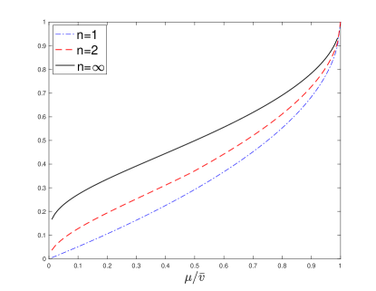
Figure 5: Competitive Ratios by $n$-Level Pricing for $n=1,2,\infty$ Under the Mean Ambiguity Set

Figure 5 depicts the comparison between competitive ratios achieved by posted price in Proposition 4.1, 2-level pricing in Proposition 4.4, and the optimal robust mechanism with continuous pricing in Proposition 4.6. We show that the improvement of the competitive ratio from 1-level pricing to 2-level pricing is significant for moderate $\mu$. Introducing a second price reduces the gap toward continuous pricing by approximately half, which demonstrates the benefits of incorporating a small menu size into robust pricing.

Now that we have discussed the competitive ratio of different mechanisms against the adversarial strategy by nature, we now evaluate the empirical performance of the 1-level pricing, 2-level pricing, and $\infty$-level pricing under given distributions. We choose beta distribution since it exhibits a variety of shapes under different parameters. We summarize the performance of the three pricing mechanisms under different shapes of valuation density functions as follows.

• For a unimodal valuation where the mode is non-zero, regardless of the valuation density being flat or concentrated, 2-level pricing exhibits superior performance. This outperformance stems from (i) the lower price in 2-level pricing effectively captures substantial revenue from the mode, as long as the mode is not significantly lower than the mean. (2) the higher price can capture the high valuations from the distribution’s right tail.

• When the valuation distribution is unimodal with a mode at zero, the 2-level and $\infty$-level pricing demonstrate comparable performance, notably surpassing the 1-level pricing. The reason for the advantage of 2-level pricing is similar to the previous scenario. Meanwhile, in this case, the $\infty$-level pricing is sometimes more effective in extracting revenue from the high valuation.

• The strengths of $\infty$-level pricing become apparent in a bimodal distribution with modes 0 and 1. In this scenario, 2-level outperforms 1-level pricing but is inferior to $\infty$-level pricing. The reason for the superiority of $\infty$-level pricing is that the dispersion of $\infty$-level pricing can capture the revenue at mode 1 effectively, yet the higher price in 2-level pricing is not as effective in extracting revenue at mode 1.

Figure 6: Performance Ratios for $n$-Level Pricing for $n=1,2,\infty$ Based on the Mean Ambiguity Set Under Beta Distributions

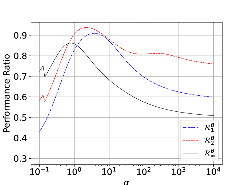
(a) $\alpha=\beta$

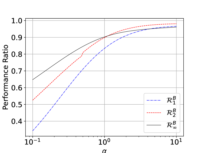
(b) $\beta=0.5$

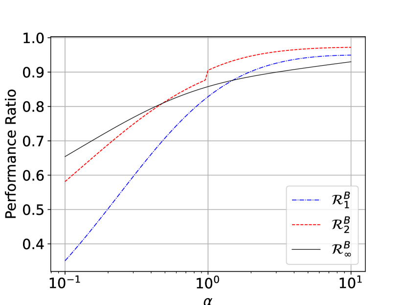
(c) $\beta=1$

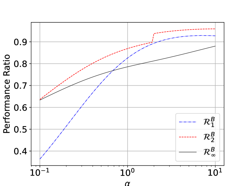
(d) $\beta=2$

Now we delve into the detailed empirical performance of the three mechanisms. When $\alpha=\beta$, in Figure 6(a), we let $\alpha=\beta$ and vary $\alpha$ from 0.1 to 10. When $\alpha=\beta<1$, the valuation density is a bimodal U-shape function with modes at 0 and 1. As $\alpha$ and $\beta$ become smaller, the valuation is more concentrated on 0 and 1, which approximates the 2-point Bernoulli distribution with an equal probability of $1/2$. In this case, as shown in Figure 6(a), the $\infty$-level pricing outperforms 1-level and 2-level pricing. The performance ratio of 1-level and 2-level pricing, especially the 1-level pricing, drops significantly as the valuation distribution degenerates to the two-point distribution, while the $\infty$-level pricing is more robust to the decreasing of $\alpha$ and $\beta$. The intuition is that the 1-level pricing can only extract about $\frac{v_{1}}{2}$ under the two-point distribution, and the 2-level pricing yields $\frac{x_{1}v_{1}+(1-x_{1})v_{2}}{2}$, while the $\infty$-level pricing spreads more evenly across the valuation, extracting more revenue from valuation 1. On the other hand, when $\alpha=\beta>1$, the valuation is a symmetric unimodal function with a mode of $1/2$. As $\alpha$ and $\beta$ become larger, the valuation is more concentrated in the mean, i.e. 0.5, and the distribution has a more similar shape to the normal distribution. Figure 6(a) indicates that as the valuation becomes more concentrated to the mean, the performance of 2-level pricing is significantly better than the other two mechanisms, and it is more robust to the increase of $\alpha$. The intuition is that as the valuation becomes more concentrated at the mean, the $\infty$-level pricing loses some revenue due to the dispersion above $\mu$, and the regret from $1$-level pricing is the gap between $v_{1}$ and the optimal pricing which approaches $\mu$. In contrast, the 2-level pricing mechanism takes advantage of the randomization between $v_{1}$ and $v_{2}$ that is slightly lower than $\mu$. Finally, when $\alpha=\beta=1$, the valuation follows a uniform distribution on $[0,1]$. Under the uniform distribution, the 2-level pricing also displays a superior performance ratio compared to 1-level and $\infty$-level pricing. This simulation highlights that a robust mechanism with a higher competitive ratio does not necessarily yield superior empirical performance under a given distribution. Nevertheless, the 2-level pricing exhibits robustness in the face of changes to the shape of the valuation distribution.

Figure 6(b) depicts the performance of 1-level, 2-level and $\infty$-level pricing as $\alpha$ ranges from 0.1 to 10 with $\beta$ set at $0.5$. When $\alpha<1$, the valuation density is U-shaped with two modes at 0 and 1. As per the previous discussion, the $\infty$-level pricing scheme demonstrates superior performance over the other two schemes. As $\alpha$ becomes greater than 1, the density function becomes unimodal with mode 1, and it is convex and increasing. As the valuation becomes more concentrated at mode 1, the 2-level pricing has a slightly higher performance than the other two schemes.

Figure 6(c) presents the performance of the three pricing schemes as $\alpha$ ranges from 0.1 to 10 and $\beta=1$. In this case, the density function becomes $\alpha x^{\alpha-1}$. For $\alpha<1$, the density has a mode 0 and is convex and decreasing. In this scenario, both the 2-level and $\infty$-level pricing schemes significantly outperform the 1-level pricing scheme. The reason is that since the density function is positively skewed with a right tail, the mean of valuation is low. Thus, the 1-level pricing has a conservative posted price that can not capture the revenue achievable from the high valuation in the right tail. In contrast, the 2-level pricing can mitigate this conservativeness effectively. As $\alpha$ becomes close to 1, the density function becomes flatter ultimately converging to a uniform distribution, and the 2-level pricing becomes more effective than the $\infty$-level pricing. As $\alpha$ becomes greater than 1, the density function becomes negatively skewed and strictly increases. It is concave, linear, and convex when $1<\alpha<2$, $\alpha=2$, and $\alpha>2$, respectively. As shown in Figure 6(c), the 2-level pricing scheme outperforms the other two selling mechanisms when $\alpha\geq 1$. As $\alpha$ increases, the valuation is more concentrated at 1, leading to all three mechanisms approaching a performance of 1.

Figure 6(d) displays the performance of the three mechanisms as $\alpha$ ranges from 0.1 to 10 and $\beta=2$. When $\alpha<1$, similar to the previous case, the density has a mode 0 and is convex and decreasing. In this scenario, the performance of 2-level pricing is more effective than the other two mechanisms. When $\alpha>1$, the density function is unimodal, and the performance of 1-level pricing increases significantly. Though it is still below the performance of 2-level pricing, it surpasses that of the $\infty$-level pricing for all $\alpha\geq 1$.

Our numerical results demonstrate the effectiveness of 2-level pricing under different shapes of distributions. The empirical performance of 2-level pricing has a significant improvement from the 1-level pricing, and 2-level pricing is more robust to parameter variations. In addition, while the competitive ratio of 2-level pricing is not as high as that of $\infty$-level pricing, the empirical performance of 2-level pricing can be superior to that of $\infty$-level pricing across many different distributions.

5 Quantile Ambiguity Set

In this section, we consider the ambiguity set $\mathcal{F}=\left\{\mathbb{F}\in\mathcal{P}([0,\bar{v}]):\,\int_{0}^{\bar{v}}\mathbbm{1}[v\geq\omega]\,d\mathbb{F}(v)\geq\xi\right\}$. This implies that based on historical sales data or market surveys, if the seller adopts a posted price at $\omega$, then the proportion of buyers who will purchase the product is at least $\xi$. Under the quantile ambiguity set, we have that $\phi(v)=\mathbbm{1}[v\geq\omega]-\xi$ and $\underline{\phi}_{j}=\lim_{v\rightarrow v_{j}-}\mathbbm{1}[v\geq\omega]-\xi=\mathbbm{1}[v_{j}>\omega]-\xi$. Hence, for any given price level set $\mathcal{V}=\{v_{1},\dots,v_{n}\}$, Problem (4) is reduced to

$$\sup\limits_{\boldsymbol{\lambda}\in\mathbb{R}^{n+1}_{+}\mathbf{x}\in\mathbb{R}_{+}^{n},r\in\mathbb{R}^{+}} r$$ (9)

$$\mathrm{s.t.} (\mathbbm{1}[v_{j}>\omega]-\xi)\lambda_{i}\leq\sum_{l=1}^{j-1}v_{l}x_{l},\ \forall\ i\in[n+1],\,j\in[i-1],$$

$$r\cdot v_{i}+(\mathbbm{1}[v_{j}>\omega]-\xi)\lambda_{i}\leq\sum_{l=1}^{j-1}v_{l}x_{l},\ \forall\ i\in[n+1],\,j=i,\dots,n+1$$

$$\sum_{i=1}^{n}x_{i}=1$$

In the following discussion, we evaluate the performance of the robust mechanisms with different levels of prices.

1-Level Pricing.

Suppose the seller posts a deterministic price at $v$. If $v>\omega$, then the worst-case distribution reduces to a single-point distribution at $\omega$, which satisfies the quantile constraint that the probability that the valuation is greater than $\omega$ is no less than $\xi\leq 1$. In this case, the revenue achieved by posting price $v$ is zero, and thus the competitive ratio is zero. Hence, we need to focus only on price $v$ that is lower than or equal to $\omega$. Then, Problem (9) reduces to the following problem:

$$\sup\limits_{\boldsymbol{\lambda}\in\mathbb{R}^{2}_{+},r\in\mathbb{R}^{+}} r$$ (10)

$$\mathrm{s.t.} r\cdot v_{1}+(-\xi)\lambda_{1}\leq 0$$

$$r\cdot v_{1}+(1-\xi)\lambda_{1}\leq v$$

$$r\cdot\bar{v}+(1-\xi)\lambda_{2}\leq v$$

In Proposition 5.1, we characterize the optimal competitive ratio achieved by 1-level pricing under the quantile ambiguity set.

Proposition 5.1

Under quantile ambiguity set $\mathcal{F}=\left\{\mathbb{F}\in\mathcal{P}([0,\bar{v}]):\,\int_{0}^{\bar{v}}\mathbbm{1}[v\geq\omega]\,d\mathbb{F}(v)\geq\xi\right\}$, the optimal competitive ratio of 1-level pricing is $\mathcal{R}_{1}=\min\left\{\xi,\ \frac{\omega}{\bar{v}}\right\}$ and the corresponding optimal posted price is $v_{1}=\min\{\omega,\xi\bar{v}\}$.

We postpone the straightforward proof to the appendix. For any fixed posted price $v_{1}\leq\omega$, nature can employ one of two possible strategies. In one scenario, the worst-case distribution of valuation can be a degenerate distribution at $\bar{v}$ (i.e., the valuation is equal to $\bar{v}$ with probability 1) and the corresponding hindsight optimal price is also $\bar{v}$. In the second scenario, nature could adopt a two-point discrete distribution: $v_{1}-$ with a probability of $1-\xi$ and $\omega$ with a probability of $\xi$, and the corresponding hindsight optimal price is $v_{1}-$. The competitive ratio in the first case is $\frac{v_{1}}{\bar{v}}$ and, in the second case, it is $\xi$. Regardless of the posted price $v_{1}$ set by the seller, nature selects the strategy that results in a lower competitive ratio. Therefore, the competitive ratio for a single fixed price ${v_{1}}$ is $\min\{\frac{v_{1}}{\bar{v}},\xi\}$. Based on nature’s strategy, the seller should opt for the maximum $v_{1}$ that does not exceed $\omega$. Moreover, when $\xi\bar{v}\leq\omega$, pricing between $\xi\bar{v}$ and $\omega$ results in the same competitive ratio. The resulting competitive ratio becomes $\mathcal{R}_{1}=\min\{\frac{\omega}{\bar{v}},\xi\}$. Notice that the worst-case distribution selected by nature always places some probability mass greater than $\omega$, so in the following, we will show that incorporating an additional price level between $v_{1}$ and $\bar{v}$ could substantially enhance the competitive ratio.

2-Level Pricing.

Suppose the seller can randomize between two prices. We aim to jointly optimize these prices, denoted as $v_{1}$ and $v_{2}$, as well as their corresponding probabilities, $x_{1}$ and $x_{2}$. The optimal pricing strategy is presented in Proposition 5.2, whose proof is postponed to the Appendix.

Proposition 5.2

Under quantile ambiguity set $\mathcal{F}=\left\{\mathbb{F}\in\mathcal{P}([0,\bar{v}]):\,\int_{0}^{\bar{v}}\mathbbm{1}[v\geq\omega]\,d\mathbb{F}(v)\geq\xi\right\}$, the optimal 2-level pricing strategy and the corresponding competitive ratio are as follows:

1. If $\xi\bar{v}\leq\omega$, then $v_{1}=\xi\bar{v}$, $v_{2}=\min\{\omega,\sqrt{\xi}\bar{v}\}$, $x_{1}=\frac{v_{2}-\xi\bar{v}}{\frac{\xi\bar{v}^{2}}{v_{2}}-2\xi\bar{v}+v_{2}}$, and $\mathcal{R}_{2}^{*}=\frac{1-\xi}{\frac{\bar{v}}{v_{2}}+\frac{v_{2}}{\xi\bar{v}}-2}$

2. If $\xi\bar{v}>\omega$, then $v_{1}=\omega$, $v_{2}=\max\{\frac{\omega}{\xi},\sqrt{\omega\bar{v}}\}$, $x_{1}=\frac{v_{2}^{2}}{v_{2}^{2}-\omega v_{2}+\omega\overline{v}}$ and $\mathcal{R}_{2}^{*}=\frac{1}{\frac{v_{2}}{\omega}+\frac{\overline{v}}{v_{2}}-1}$.

Notice that in the 2-level pricing scheme, the optimal pricing strategy satisfies that the lower price level $v_{1}=\min\{\omega,\xi\bar{v}\}$ which is equal to the optimal price in 1-level pricing. Now we hope to see how the competitive ratio is increased by incorporating 2-level pricing. For notational simplicity, we denote $\bar{v}=1$. If $\xi\bar{v}\leq\omega$, then $\mathcal{R}_{1}^{*}=\xi,\mathcal{R}_{2}^{*}=\frac{\xi(1-\xi)}{\frac{\xi}{v_{2}}-2\xi+v_{2}}$ and $\mathcal{R}_{2}^{*}/\mathcal{R}_{1}^{*}=\frac{(1-\xi)\xi}{\frac{v_{1}^{2}}{v_{2}}-2\xi v_{1}+\xi v_{2}}=\frac{(1-\xi)}{\frac{\xi}{v_{2}}-2\xi+v_{2}}$. When $\omega\geq\sqrt{\xi}\bar{v}$, we have that $\mathcal{R}_{2}^{*}/\mathcal{R}_{1}^{*}=\frac{(1-\xi)}{2(\sqrt{\xi}-\xi)}=\frac{1}{2}(1+\frac{1}{\sqrt{\xi}})$. Hence, we observe that when $\xi$ is small, the improvement is more significant.

$\infty$-Level Pricing.

In the following, we obtain the benchmark where the seller can adopt the optimal robust mechanism by solving Problem (3) with the feasible mechanism set $\mathcal{X}=\{x:[0,\bar{v}]\rightarrow\mathbb{R}^{+}\,\mid\,\int_{0}^{\bar{v}}x(u)du=1\}$. Under the quantile ambiguity set, Problem (3) becomes the following infinite linear programming:

$$\sup\limits_{\boldsymbol{\lambda}\in\mathbb{R}^{[0,\bar{v}]}_{+},\ \mathbf{x}\in\mathcal{X},\ r\in\mathbb{R}^{+}} r$$ (11)

$$\mathrm{s.t.} \mathbbm{1}[v\geq\omega]\cdot\lambda(p)-\xi\cdot\lambda(p)\leq\int_{0}^{v}x(u)u\,du\quad\forall p\in[0,\bar{v}],\ \forall v\in[0,p),$$

$$r\cdot p+\mathbbm{1}[v\geq\omega]\cdot\lambda(p)-\xi\cdot\lambda(p)\leq\int_{0}^{v}x(u)u\,du\quad\forall p\in[0,\bar{v}],\ \forall v\in[p,\bar{v}].$$

$$\int_{0}^{\bar{v}}x(v)\,dv=1$$

In Proposition 5.3, we characterize the optimal robust selling mechanism and optimal competitive ratio with no menu-size constraints.

Proposition 5.3

Under quantile ambiguity set $\mathcal{F}=\left\{\mathbb{F}\in\mathcal{P}([0,\bar{v}]):\,\int_{0}^{\bar{v}}\mathbbm{1}[v\geq\omega]\,d\mathbb{F}(v)\geq\xi\right\}$, the optimal price density function $x(v)$ and the corresponding payment function $t(v)$ are defined as follows:

$$\begin{cases}x(v)=\begin{cases}\frac{r}{(1-\xi)v}&\forall v\in[\xi\widehat{p},\omega)\\ \frac{r}{v}&\forall v\in[\widehat{p},\bar{v}]\\ \end{cases}\\ x(v)\,\text{has a probability mass of }\frac{r(\widehat{p}-\omega)}{\omega(1-\xi)}\text{ at }\omega\end{cases}\quad t(v)=\int_{0}^{v}x(u)u\,du=\begin{cases}0&\forall v\in[0,\xi\widehat{p})\\ \frac{r\cdot(v-\xi\widehat{p})}{1-\xi}&\forall v\in[\xi\widehat{p},\omega)\\ r\cdot\widehat{p}&\forall v\in[\omega,\widehat{p})\\ r\cdot v&\forall v\in[\widehat{p},\bar{v}]\\ \end{cases}$$

where $\widehat{p}=\min\{(2-\xi)\omega,\bar{v}\}$, and the corresponding competitive ratio is

$$r=\begin{cases}\big{(}\ln(\bar{v})-\ln(\omega(2-\xi))-\frac{\ln(\xi(2-\xi))}{1-\xi}+1\big{)}^{-1}&\mbox{if }\ (2-\xi)\omega<\bar{v}\\ \big{(}\frac{\bar{v}-\omega}{(1-\xi)\omega}+\frac{\ln(\omega)-\ln(\xi\bar{v})}{1-\xi}\big{)}^{-1}&\mbox{if }\ (2-\xi)\omega\geq\bar{v}.\end{cases}$$

Suppose a firm can post a price at $\omega$ and observe the market response, i.e., the proportion $\xi$ of customers in the market it attracts. Proposition 5.3 suggests that for fixed posted price $\omega$, the competitive ratio is increasing in the market penetration.

Corollary 5.4

For fixed posted price $\omega$, the competitive ratio is increasing in the market share $\xi$.

According to Corollary 5.4, an increase in the probability of customers’ valuation being no less than $\omega$ reduces the ambiguity set of worst-case distributions that nature can choose from. As a result, a larger market share $\xi$ yields a more favorable competitive ratio.

Moreover, Proposition 5.3 implies the allocation function (or the cumulative price distribution function) is defined as

$$q(v)=\int_{0}^{v}x(u)\,du=\begin{cases}0&\forall v\in[0,\xi\widehat{p})\\ \frac{r}{1-\xi}\ln\frac{v}{\xi\widehat{p}}&\forall v\in[\xi\widehat{p},\omega)\\ 1-r\ln(\bar{v}/\widehat{p})&\forall v\in[\omega,\widehat{p})\\ 1-r\ln(\bar{v}/v)&\forall v\in[\widehat{p},\bar{v}].\end{cases}$$

Based on the characterization of $x(v)$ and $q(v)$, we show that when the market share $\xi$ increases, the seller prices at higher valuations with greater probability.

Corollary 5.5

Given a posted price $\omega$, if $\xi^{{\dagger}}\leq\xi^{{\ddagger}}$, then the optimal pricing strategy $x^{{\dagger}}$ derived from market share $\xi^{{\dagger}}$ is stochastically dominated by the optimal pricing strategy $x^{{\ddagger}}$ derived from market share $\xi^{{\ddagger}}$.

Corollary 5.5 is intuitive because as the proportion of customers who accept price $\omega$ increases, the seller is more confident about the customers’ valuation of the product. Hence, the pricing strategy derived from a higher market share $\xi^{{\ddagger}}$ is less conservative than the pricing strategy derived from a lower market share $\xi^{{\dagger}}$.

Figure 7: Competitive Ratio for $n$-Level Pricing for $n=1,2$ and Infinity Under the Quantile Ambiguity Set

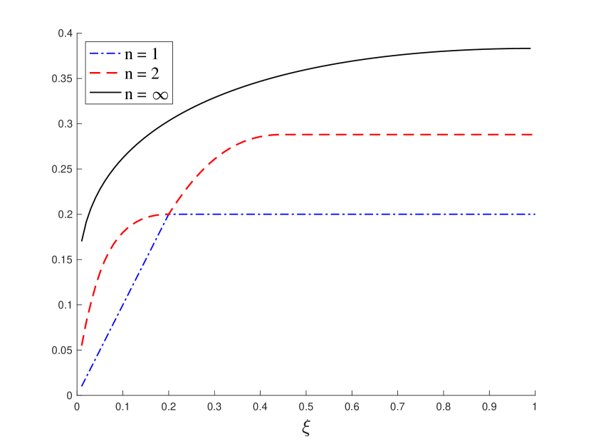
(a) $\omega/\bar{v}=0.2$

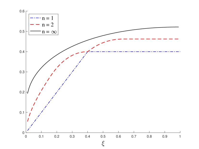
(b) $\omega/\bar{v}=0.4$

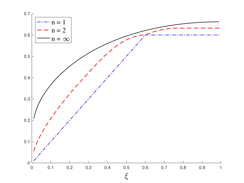
(c) $\omega/\bar{v}=0.6$

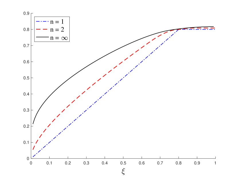
(d) $\omega/\bar{v}=0.8$

Comparison of 1-Level, 2-Level and $\infty$-Level Pricing.

In Figure 7, we compare the competitive ratio achieved by 1-level pricing as defined in Proposition 5.1, 2-level pricing as defined in Proposition 5.2 and the $\infty$-level pricing (optimal robust mechanism) as defined in Proposition 5.3. We consider various quantile information with $\omega/\bar{v}$ ranging from $0.2$ to $0.8$, and $\xi$ varying from 0 to 1. Figure 7 shows that the improvement of the 2-level pricing is significant compared to 1-level pricing. This improvement becomes even more pronounced as $\xi$ approaches zero, where 2-level pricing can outperform 1-level pricing by several folds. Moreover, when $\omega/\bar{v}$ is moderate or large, the competitive ratio achieved by the 2-level pricing is very close to that achieved by the optimal robust mechanism, especially when $\xi$ is greater than $\omega/\bar{v}$. These observations underline the potential advantages of implementing a 2-level pricing strategy over 1-level pricing.

Now that we have characterized the competitive ratio for different selling schemes, we now proceed to assess the empirical performance of these mechanisms. Our analysis employs similar distributions as presented in Section 4.2, specifically using Beta distributions with $\beta$ values of 0.5, 1, and 2, while varying $\alpha$ between 0.1 and 10. For each Beta distribution, we generate $(1-\xi)$-quantiles for $\xi$ values of 0.3, 0.5, and 0.7, and then the robust selling mechanisms are designed based on these quantile values. The main insights from the empirical performance are outlined below, followed by detailed discussions.

• When the valuation distribution does not have a mode at zero, then it is more beneficial to leverage the information of a moderate or large quantile level $\xi$, which yields high performance for all three robust mechanisms.

• When the valuation distribution presents two modes at 0 and 1 and negative skew, 2-level pricing, and $\infty$-level pricing both have good performance, irrespective of whether $\xi$ is small, moderate, or large.

• In cases where the valuation distribution has two modes at 0 and 1 with positive skew, it is advantageous to utilize information from a small or moderate quantile level $\xi$. While 2-level pricing and $\infty$-level pricing outperform the 1-level pricing, none of the robust mechanisms perform very well in this scenario.

• Across all types of distributions, the performance of 2-level pricing is robust to the choice of quantile-level information.

Figure 8: Performance Ratio for $n$-Level Pricing for $n=1,2$ and Infinity Based the Quantile Ambiguity Set Under Beta Distributions

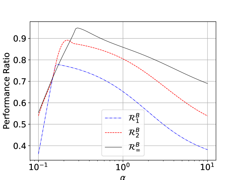
(a) $\beta=0.5,\xi=0.3$

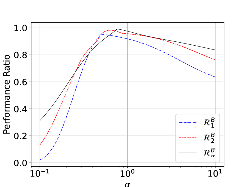
(b) $\beta=0.5,\xi=0.5$

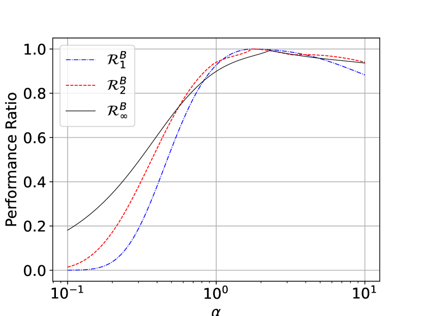
(c) $\beta=0.5,\xi=0.7$

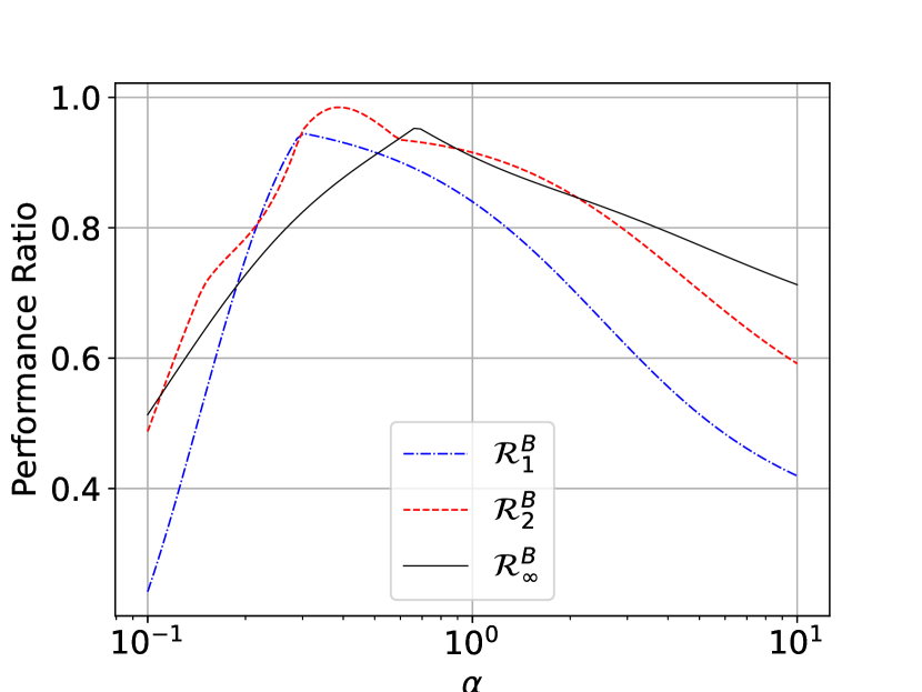
(d) $\beta=1,\xi=0.3$

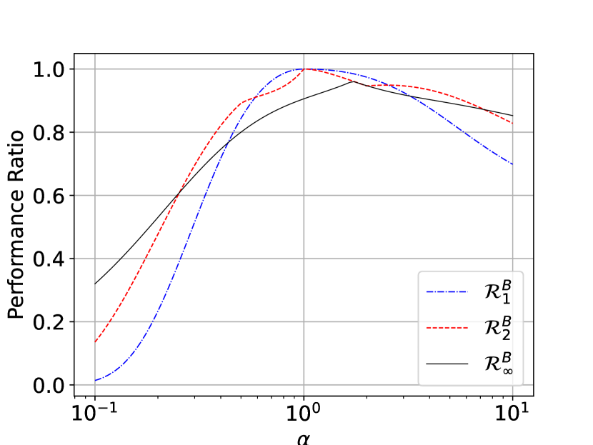
(e) $\beta=1,\xi=0.5$

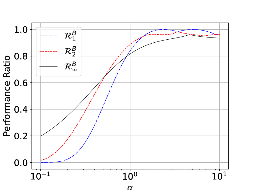
(f) $\beta=1,\xi=0.7$

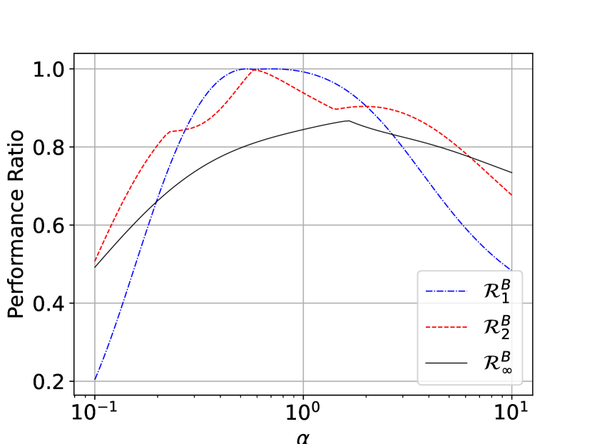
(g) $\beta=2,\xi=0.3$

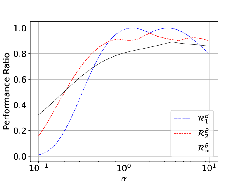
(h) $\beta=2,\xi=0.5$

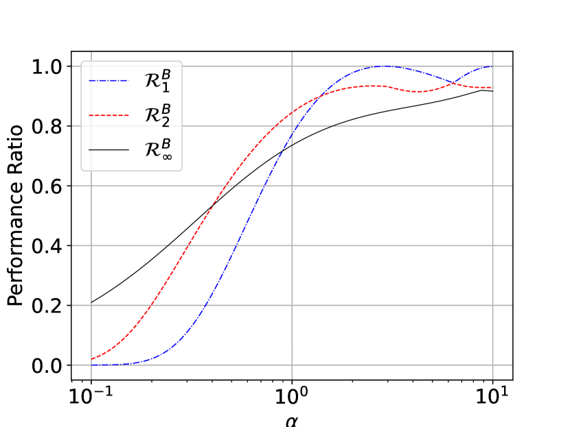
(i) $\beta=2,\xi=0.7$

In Figure 8, we observe that when $\alpha$ is small, the valuation distribution has a mode at 0 or two modes at 0 and 1. Given this configuration, the $(1-\xi)$-quantile tends to be small, meaning that a robust mechanism based on a near-zero quantile $\omega$ does not assure substantial revenue. Consequently, none of the three robust mechanisms has a good performance in this scenario. For $\beta=0.5$ and $\alpha$ approximating or exceeding 1, the valuation distribution mode shifts to 1. In these cases, adopting a moderate or large quantile level $\xi$, such as $\xi=0.5$ or $\xi=0.7$, consistently leads to good performance for all the robust selling mechanisms. For small $\xi=0.3$, the performance of the $\infty$-level pricing and 2-level pricing is more robust to the increase of $\alpha$. This is attributed to the fact that for small $\xi$, even if the $(1-\xi)$-quantile is large, the 1-level pricing posts price at $\xi$, which results in a revenue loss. In contrast, in 2-level pricing, even though the lower price is also at $\xi$, the higher price set at $\min\{\omega,\sqrt{\xi}\}$ can extract the revenue at valuation $\sqrt{\xi}$ efficiently.

When $\beta=1$ or $\beta=2$, and $\alpha$ is not very close to 0.1, the performance of 1-level pricing and 2-level pricing outperform $\infty$-level pricing under moderate $\alpha$ for any choice of quantile information. On the other hand, $\infty$-level pricing outperforms 1-level pricing and 2-level pricing for large $\alpha$ and small $\xi$. The reason that 1-level and 2-level pricing have superior performance under moderate $\alpha$ and $\beta$ is that in these scenarios, the valuation distribution is a single mode so adopting a moderate or large $\xi$ can secure a large amount of revenue captured by the mode in the distribution. Similarly, the performance is inferior if the valuation distribution has a mode at 0. In light of the numerical results, we can see that the 2-level pricing is very robust to the choice of quantile level $\xi$ across different distributions.

6 Summary and Future Directions

In this paper, we introduce the $n$-level pricing problems that establish a favorable balance between theoretical robustness and practical implementation. We propose a unified framework that can address a broad class of ambiguity sets including support, mean, and quantile information. Our framework enables us to derive closed-form representations of the optimal $n$-level pricing mechanism and the corresponding competitive ratio under the support ambiguity set. Moreover, we provide closed-form characterizations of the optimal selling mechanism and the corresponding competitive ratio for 1-level pricing and 2-level pricing under the mean ambiguity set. Furthermore, we characterize the optimal selling mechanism and the corresponding competitive ratio for 1-level pricing, 2-level pricing, and $\infty$-level pricing under the quantile ambiguity set. Our closed-form competitive ratios in different mechanisms shed light on the effectiveness of 2-level pricing compared to 1-level pricing. Although our primary focus has been the support, mean and quantile ambiguity sets, our framework allows for an extension to more general ambiguity sets. Our major implication is that merely randomizing between just two prices can significantly improve the performance of deterministic pricing. One of the most interesting future explorations would be to quantify the competitive ratio for general $n$-level pricing under different ambiguity sets, which could provide deeper insights on how the performance guarantee of a robust mechanism depends on the menu complexity.

7 Proof in Section 2

Proof 7.1

Proof of Proposition 2.1. Problem (1) can be represented as $\sup_{\mathbf{x}\in\mathcal{X}_{n}}\mathrm{CR}(\mathbf{x})=\sup\limits_{\mathbf{x}\in\mathcal{X}_{n}}\inf\limits_{\mathbb{F}\in\mathcal{F}}\min\limits_{p\in[0,\bar{v}]}\frac{\int_{0}^{\bar{v}}(\int_{0}^{v}x(u)u\,du)\,d\mathbb{F}(v)}{p(1-\mathbb{F}(p-))}$, so we can exchange the order of minimization. Hence, Problem (1) is equivalent to

$$\sup_{\mathbf{x}\in\mathcal{X}_{n}}\mathrm{CR}(\mathbf{x})=\sup_{\mathbf{x}\in\mathcal{X}_{n}}\min_{p\in[0,\bar{v}]}\inf_{\mathbb{F}\in\mathcal{F}}\ \frac{\int_{0}^{\bar{v}}(\int_{0}^{v}x(u)u\,du)\,d\mathbb{F}(v)}{p(1-\mathbb{F}(p-))}$$

Denoting $r=\mathrm{CR}(\mathbf{x})$, we have the following equivalent formulation to the above problem.

$$\sup_{r\in\mathbb{R}_{+},\mathbf{x}\in\mathcal{X}_{n}} r$$

s.t. $$r\cdot p\ \leq\ \inf_{\mathbb{F}\in\mathcal{F}}\ \frac{\int_{0}^{\bar{v}}(\int_{0}^{v}x(u)u\,du)\,d\mathbb{F}(v)}{(1-\mathbb{F}(p-))},\quad\forall p\in[0,\bar{v}]$$ (12)

Incorporating the definition of $\mathcal{F}$ defined in (2), the infimum problem on the right-hand side of constraint (12) for each $p\in[0,\bar{v}]$ can be written in the following problem:

$$\begin{aligned} \displaystyle\inf_{\mathbb{F}:[0,\bar{v}]\rightarrow[0,1]}\quad&\frac{\int_{0}^{\bar{v}}(\int_{0}^{v}x(u)u\,du)\,d\,\mathbb{F}(v)}{1-\mathbb{F}(p-)}\\ \mathrm{s.t.}\quad&\int_{v\in[0,\bar{v}]}\,d\,\mathbb{F}(v)=1\\ &\int_{v\in[0,\bar{v}]}\phi_{k}(v)\,d\,\mathbb{F}(v)\geq 0,\ \forall k=1,2\ldots,K.\end{aligned}$$

Then we introduce new decision variables $H_{p}(v)=\frac{\mathbb{F}(v)}{1-\mathbb{F}(p-)}$, in order to get rid of the nonlinear objective, and the problem above is equivalent to a linear programming:

$$\begin{aligned} \displaystyle\inf_{dH_{p}\geq 0}\quad&\int_{0}^{\bar{v}}(\int_{0}^{v}x(u)u\,du)\,d\,H_{p}(v)\\ \mathrm{s.t.}\quad&\int_{v\in[p,\bar{v}]}\,d\,H_{p}(v)=1\\ &\int_{v\in[0,\bar{v}]}\phi_{k}(v)\,d\,H_{p}(v)\geq 0,\ \forall\ k=1,2\ldots,K.\end{aligned}$$

By Sion’s theorem (Sion 1958), the optimal objective value for the above problem is equal to that of its dual problem. Let $\boldsymbol{\lambda}_{p}=(\lambda_{0}(p),\lambda_{1}(p),\dots,\lambda_{K}(p))\in\mathbb{R}\times\mathbb{R}^{K}_{+}$ be the dual variables associated with the problem above. The dual problem can be formulated as follows:

$$\begin{aligned} \displaystyle\max_{\boldsymbol{\lambda}_{p}\in\mathbb{R}\times\mathbb{R}^{K}_{+}}\quad&\lambda_{0}(p)\\ \mathrm{s.t.}&\sum_{k=1}^{K}\phi_{k}(v)\lambda_{k}(p)\leq\int_{0}^{v}x(u)u\,du\quad\forall v\in[0,p)\\ &\lambda_{0}(p)+\sum_{k=1}^{K}\phi_{k}(v)\lambda_{k}(p)\leq\int_{0}^{v}x(u)u\,du\quad\forall v\in[p,\bar{v}]\end{aligned}$$

Substituting the right-hand side of constraint (12) with the above maximization problem, we have that

$$\sup_{\boldsymbol{\lambda}\in\mathbb{R}^{(K+1)\times[0,\bar{v}]}_{+},r\in\mathbb{R}_{+},\mathbf{x}\in\mathcal{X}_{n}} r$$

s.t. $$r\cdot p\ \leq\ \lambda_{0}(p),\quad\forall p\in[0,\bar{v}]$$

$$\sum_{k=1}^{K}\phi_{k}(v)\lambda_{k}(p)\leq\int_{0}^{v}x(u)u\,du\quad\forall p\in[0,\bar{v}],\,v\in[0,p)$$

$$\lambda_{0}(p)+\sum_{k=1}^{K}\phi_{k}(v)\lambda_{k}(p)\leq\int_{0}^{v}x(u)u\,du\quad\forall p\in[0,\bar{v}],\,v\in[p,\bar{v}]$$

Notice that $\lambda_{0}(p)$ can be eliminated by letting $\lambda_{0}(p)=r\cdot p$, and then the problem above becomes Problem (3), which completes our proof of Proposition 2.1.  $\square$

Proof 7.2

Proof of Theorem 2.2. Problem (3) has an infinite number of constraints characterized by an infinite sequence of $p\in[0,\bar{v}]$ and $v\in[0,\bar{v}]$. To reduce the number of constraints, we first prove the redundancy of most constraints indexed by $v$. We demonstrate that based on the optimal choice of $\boldsymbol{\lambda}\in\mathbb{R}^{K\times[0,\bar{v}]}_{+}$, the number of potentially active constraints is finite. To reduce the number of decision variables indexed by $p\in[0,\bar{v}]$, we prove the existence of an optimal solution to Problem (3), wherein $\lambda_{k}(p)$ is a piecewise constant function of $p$. In particular, the set of distinct values that $\lambda_{k}(p)$ can take over the domain $p\in[0,\bar{v}]$ is finite. In this way, we are able to reduce both the dimension of decision variables and that of constraints to finite.

Given the price level set $\mathcal{V}=\{v_{1},v_{2},\dots,v_{n}\}$, we denote $x_{i}$ the probability that the seller posts a price at $v_{i}$ for all $i=1,\dots,n$, and then the payment function can be represented by a step function of $v$. Specifically, the right-hand side of the constraints in Problem (3) satisfies $\int_{0}^{v}x(u)u\,du=\sum_{l=1}^{j}x_{l}v_{l}$, if $v\in[v_{j},v_{j+1})$ for all $j=0,1,\dots,n+1$. Embedding this relationship into the right-hand side of the constraints in (3), we have an equivalent formulation of (3) as follows. Here we denote $v_{0}=0,v_{n+1}=\bar{v}$, and $j(v)=\operatorname*{arg\,max}_{j=0,1,\dots,n}v\geq v_{j}$.

$$\sup\limits_{\boldsymbol{\lambda}\in\mathbb{R}^{K\times[0,\bar{v}]}_{+},\ \mathbf{x}\in\mathbb{R}_{+}^{n},\ r\in\mathbb{R}^{+}} r$$

$$\mathrm{s.t.} \sum_{k=1}^{K}\phi_{k}(v)\lambda_{k}(p)\leq\sum_{l=1}^{j(v)}x_{l}v_{l}\quad\forall p\in[0,\bar{v}],\ v\in[0,p)$$

$$r\cdot p+\sum_{k=1}^{K}\phi_{k}(v)\lambda_{k}(p)\leq\sum_{l=1}^{j(v)}x_{l}v_{l}\quad\forall p\in[0,\bar{v}],\ \forall v\in[p,\bar{v}]$$

$$\sum_{i=1}^{n}x_{i}=1$$

Due to Proposition 2.1, since each $\phi_{k}(v)$ is piecewise continuous with $\mathcal{B}$ as the joint set of breakpoints, we have that for all $\boldsymbol{\lambda}$, $\sum_{k=1}^{K}\phi_{k}(v)\lambda_{k}(p)$ is also piecewise continuous with breakpoints taking values from $\mathcal{B}$. At the same time, since $\phi_{k}(\cdot)$ is nondecreasing within each segment, for all $\boldsymbol{\lambda}\geq\boldsymbol{0}$, $\sum_{k=1}^{K}\phi_{k}(v)\lambda_{k}(p)$ is also nondecreasing within each segment. Notice that the right-hand side $\sum_{l=1}^{j(v)}x_{l}v_{l}$ is a piecewise constant function of $v$, so the difference between them $\sum_{k=1}^{K}\phi_{k}(v)\lambda_{k}(p)-\sum_{l=1}^{j(v)}x_{l}v_{l}$ is a piecewise continuous function that is nondecreasing within each segment. Besides, the function added by a constant term $r\cdot p$ also satisfies this property, which corresponds to the second set of constraints $r\cdot p+\sum_{k=1}^{K}\phi_{k}(v)\lambda_{k}(p)-\sum_{l=1}^{j(v)}x_{l}v_{l}$. Though the constraints require the negativity of an infinite number of piecewise increasing functions indexed by $p\in[0,\bar{v}]$, each piecewise increasing function achieves its maximum at the right endpoint in each segment. Therefore, the only active constraints in the above optimization problem are indexed by $v\rightarrow u_{j}-$ for some $u_{j}\in\mathcal{V}\cup\mathcal{B}\cup\{\bar{v}\}$. Hence, we reduce the number of constraints and obtain an equivalent formulation as follows:

$$\sup\limits_{\boldsymbol{\lambda}\in\mathbb{R}^{K\times[0,\bar{v}]}_{+},\ \mathbf{x}\in\mathbb{R}_{+}^{n},\ r\in\mathbb{R}^{+}} r$$

$$\mathrm{s.t.} \sum_{k=1}^{K}\underline{\phi}_{k,j}\lambda_{k}(p)\leq\sum_{l\in S_{j}}x_{l}v_{l}\quad\forall p\in[0,\bar{v}],\ j=1,\dots,j(p)$$

$$r\cdot p+\sum_{k=1}^{K}\underline{\phi}_{k,j}\lambda_{k}(p)\leq\sum_{l\in S_{j}}x_{l}v_{l}\quad\forall p\in[0,\bar{v}],\ j=j(p)+1,\dots,n+m+1$$

$$\sum_{i=1}^{n}x_{i}=1.$$

where $S_{j}=\{l=1,\dots,n\mid v_{l}<u_{j}\}$ for $j=1,\dots,n+m+1$ and $j(p)=\operatorname*{arg\,max}_{j}v_{j}\leq p$. Next, we aim to reduce the dimension of decision variables $\boldsymbol{\lambda}\in\mathbb{R}^{K\times[0,\bar{v}]}_{+}$. For any $i=0,1,\dots,n+m$, the constraints corresponding to $\boldsymbol{\lambda}(p)$ for $p\in[u_{i},u_{i+1})$ are represented as

$$\sum_{k=1}^{K}\underline{\phi}_{k,j}\lambda_{k}(p)\leq\sum_{l\in S_{j}}x_{l}v_{l}\quad\forall\ j\in[i]$$ (13a)

$$r\cdot p+\sum_{k=1}^{K}\underline{\phi}_{k,j}\lambda_{k}(p)\leq\sum_{l\in S_{j}}x_{l}v_{l}\quad\forall\ j=i+1,\dots,n+m+1.$$ (13b)

Notice that for each constraint with the same index $j$, the right-hand side $\sum_{l\in S_{j}}x_{l}v_{l}$ is the same regardless of $p$. At the same time, the coefficient for $\lambda_{k}(p)$ on the left-hand side, $\underline{\phi}_{k,j}$ is the same for all $p\in[u_{i},u_{i+1})$. Thus, for the constraints with the same indexed by $j$, the only difference in the constraints across different $p$ lies in the term $r\cdot p$. Since $r\cdot p$ is increasing in $p$, any feasible variable $\{\lambda_{k}(u_{i+1}-)\}_{k=1}^{K}$ satisfying the following constraints

$$\sum_{k=1}^{K}\underline{\phi}_{k,j}\lambda_{k}(u_{i+1}-)\leq\sum_{l\in S_{j}}x_{l}v_{l}\quad\forall\ j\in[i]$$

$$r\cdot u_{i+1}+\sum_{k=1}^{K}\underline{\phi}_{k,j}\lambda_{k}(u_{i+1}-)\leq\sum_{l\in S_{j}}x_{l}v_{l}\quad\forall\ j=i+1,\dots,n+m+1$$

is also feasible for all constraints in (13a) and (13b) for any $p\in[u_{i},u_{i+1})$. Thus, we could let $\lambda_{k}(p)=\lambda_{k}(u_{i+1}-)$ for all $p\in[u_{i},u_{i+1})$, and satisfying the constraints corresponding to $p=u_{i+1}-$ implies the feasibility of all other constraints indexed by $p\in[u_{i},u_{i+1})$. Hence, it is sufficient to determine the decision variables $\boldsymbol{\lambda}_{k}(\cdot)$ indexed by the right endpoints of all segments partitioned by the valuations in $\mathcal{V}\cup\mathcal{B}$. The above analysis indicates that any feasible solution $\boldsymbol{\lambda}_{k}(\cdot)$ can be represented as a piecewise constant function of $p$, whose range contains at most $n+m+1$ values. Therefore, we can reduce the dimension of decision variables $\boldsymbol{\lambda}$ to $K\times(n+m+1)$. Hence, incorporating all constraints for $i\in[n+m+1]$ and slightly reindexing the constraints provides the equivalent formulation in problem (4).  $\square$

8 Proof in Section 3

Proof 8.1

Proof of Lemma 3.1. As discussed above, if $v_{1}>\underline{v}$, then $r=0$, so we must have $v_{1}=\underline{v}$. Hence, constraint (5b) becomes $r\cdot v_{1}\leq x_{1}\cdot v_{1}$, which is implied by the first constraint in (5a), i.e., $r\cdot v_{2}\leq x_{1}\cdot v_{1}$. Therefore, the optimal competitive ratio $r$ solved by Problem (5) is equivalent to

$$r=\min_{i=2,\dots,n+1}\left\{\frac{\sum_{j=1}^{i-1}x_{j}\cdot v_{j}}{v_{i}}\right\}$$

For fixed $x_{1},x_{2},\dots,x_{t-1}$, let us define

$$f_{t}(y\mid x_{1},x_{2},\dots,x_{t-1})=\max_{\{x_{t},\dots,x_{n}\mid\sum_{j=t}^{n}x_{j}\leq y\}}\min_{i=t+1,\dots,n+1}\left\{\frac{\sum_{j=1}^{i-1}x_{j}\cdot v_{j}}{v_{i}}\right\}$$

Then we have that

$$f_{t}(y\mid x_{1},x_{2},\dots,x_{t-1})=\max_{0\leq x_{t}\leq y}\min\left\{\frac{\sum_{j=1}^{t}x_{j}\cdot v_{j}}{v_{t+1}},\ \,f_{t+1}(y-x_{t}\mid x_{1},\dots,x_{t-1},x_{t})\right\}$$

Next we show that the second term is decreasing in $x_{t}$. For any $x_{t}$, suppose the optimal solution to problem $f_{t+1}(y-x_{t}\mid x_{1},x_{2},\dots,x_{t-1},x_{t})$ is $x_{t+1},\dots,x_{n}$. Then consider solution $x_{t}^{\prime}=x_{t}-\epsilon$, $x_{t+1}^{\prime}=x_{t+1}+\epsilon,x_{i}^{\prime}=x_{i},\,\forall i\geq t+2$. Since $\frac{\sum_{j=1}^{i-1}x_{j}^{\prime}\cdot v_{j}}{v_{i}}=\frac{\sum\limits_{j<i,j\neq t,t+1}x_{j}^{\prime}\cdot v_{j}+(x_{t}-\epsilon)v_{t}+(x_{t+1}+\epsilon)v_{t+1}}{v_{i}}=\frac{\sum\limits_{j<i}x_{j}\cdot v_{j}+\epsilon(v_{t+1}-v_{t})}{v_{i}}>\frac{\sum_{j=1}^{i-1}x_{j}\cdot v_{j}}{v_{i}}$, for any $i\geq t+2$, we have that $\min\limits_{i=t+2,\dots,n+1}\left\{\frac{\sum_{j=1}^{i-1}x_{j}^{\prime}\cdot v_{j}}{v_{i}}\right\}\geq\min\limits_{i=t+2,\dots,n+1}\left\{\frac{\sum_{j=1}^{i-1}x_{j}\cdot v_{j}}{v_{i}}\right\}$. It follows that

$$f_{t+1}(y-x_{t}^{\prime}\mid x_{1},\dots,x_{t-1},x_{t}^{\prime}) = \max_{\{x_{t+1},\dots,x_{n}\mid\sum_{j=t+1}^{n}x_{j}\leq y-x_{t}^{\prime}\}}\min_{i=t+2,\dots,n+1}\left\{\frac{\sum_{j=1}^{i-1}x_{j}\cdot v_{j}}{v_{i}}\right\}$$

$$\geq \min_{i=t+2,\dots,n+1}\left\{\frac{\sum_{j=1}^{i-1}x_{j}^{\prime}\cdot v_{j}}{v_{i}}\right\}$$

$$\geq \min_{i=t+2,\dots,n+1}\left\{\frac{\sum_{j=1}^{i-1}x_{j}\cdot v_{j}}{v_{i}}\right\}$$

$$= f_{t+1}(y-x_{t}\mid x_{1},\dots,x_{t-1},x_{t})$$

which implies that $f_{t+1}(y-x_{t}\mid x_{1},\dots,x_{t-1},x_{t})$ is decreasing in $x_{t}$. Now that $\frac{\sum_{j=1}^{t}x_{j}\cdot v_{j}}{v_{t+1}}$ is increasing in $x_{t}$ and $f_{t+1}(y-x_{t}\mid x_{1},\dots,x_{t-1},x_{t})$ is decreasing in $x_{t}$, the optimal $x_{t}$ equates the two terms in order to maximize the minimum of the two terms. Therefore, we have proved that $\frac{\sum_{j=1}^{t}x_{j}\cdot v_{j}}{v_{t+1}}=\frac{\sum_{j=1}^{t+1}x_{j}\cdot v_{j}}{v_{t+2}}$ for any $t$ by backward induction, so we have that

$$r=\frac{x_{1}\cdot v_{1}}{v_{2}}=\dots=\frac{\sum_{j=1}^{i}x_{j}\cdot v_{j}}{v_{i+1}}=\dots=\frac{\sum_{j=1}^{n}x_{j}\cdot v_{j}}{v_{i+1}}$$

Hence, the optimal pricing probabilities are given by $x_{1}=r\cdot\frac{v_{2}}{\underline{v}},\,x_{i}=r\cdot\frac{v_{i+1}-v_{i}}{v_{i}},\,\forall\ i=2,\dots,n$. Taking into account $\sum_{i=1}^{n}x_{i}=1$, we have that $r=\big{(}\frac{v_{2}}{v_{1}}+\sum_{i=2}^{n}\frac{v_{i+1}-v_{i}}{v_{i}}\big{)}^{-1}$.

Proof 8.2

Proof of Proposition 3.2. The optimal competitive ratio can be represented as $r=\big{(}\frac{v_{2}}{v_{1}}+\sum_{i=2}^{n}\frac{v_{i+1}-v_{i}}{v_{i}}\big{)}^{-1}=\big{(}\sum_{i=1}^{n}\frac{v_{i+1}}{v_{i}}-(n-1)\big{)}^{-1}$. Given that $v_{1}=\underline{v},v_{n+1}=\bar{v}$ are fixed, we now consider how $r$ changes with $v_{i}$ for $i=2,\dots,n$. The derivative of $\sum_{i=1}^{n}\frac{v_{i+1}}{v_{i}}$ with respect to $v_{i}$ is $-\frac{v_{i+1}}{v_{i}^{2}}+\frac{1}{v_{i-1}}$, which implies that $\sum_{i=1}^{n}\frac{v_{i+1}}{v_{i}}$ is decreasing in $v_{i}$ if $v_{i}\leq\sqrt{v_{i-1}{v_{i+1}}}$ and increasing in $v_{i}$ if $v_{i}\geq\sqrt{v_{i-1}{v_{i+1}}}$. Hence, the optimal $v_{i}$ satisfies $v_{i}=\sqrt{v_{i-1}{v_{i+1}}}$ for all $i=2,\dots,n$. It follows that $v_{i}=\underline{v}\cdot(\bar{v}/\underline{v})^{\frac{i-1}{n}}=\underline{v}^{\frac{n+1-i}{n}}\cdot\bar{v}^{\frac{i-1}{n}}$, for all $i=1,\dots,n$. Then by Lemma 3.1, we obtain the optimal pricing probabilities for different price levels.  $\square$

9 Proofs in Section 4

Proof 9.1

Proof of Proposition 4.1. Notice that when $v_{1}>\mu$, since $\lambda_{1}\geq 0$, the first constraint implies $r\cdot v_{1}\leq 0$, suggesting $r\leq 0$. Besides, $r=0,\lambda_{1}=0$ forms a feasible solution to the above problem, so when $v_{1}>\mu$, the optimal competitive ratio achieved by a deterministic posted price $v_{1}$ is $0$. Subsequently, our analysis will focus on characterizing the non-trivial optimal solution for the scenario $v_{1}\leq\mu$.

In the case where $v_{1}\leq\mu$, the first constraint in (7) can be rewritten as $\lambda_{1}\geq\frac{r\cdot v_{1}}{\mu-v_{1}}$ and the second constraint can be rewritten as $\lambda_{1}\leq\frac{v_{1}-r\cdot v_{1}}{\bar{v}-\mu}$. For a feasible solution $\lambda_{1}$ to exist, the intersection of these two conditions results in $r\leq\frac{\mu-v_{1}}{\bar{v}-v_{1}}$. Taking into account the third constraint $r\leq\frac{v_{1}}{\bar{v}}$, we have that the optimal objective value $r$ in Problem (7) is

$$\mathcal{R}(\{v_{1}\})=\min\{\frac{v_{1}}{\bar{v}},\frac{\mu-v_{1}}{\bar{v}-v_{1}}\}$$

Consequently, the optimal posted price selling scheme is deduced by $v_{1}^{*}=\operatorname*{arg\,max}_{v_{1}}\{\min\{\frac{v_{1}}{\bar{v}},\frac{\mu-v_{1}}{\bar{v}-v_{1}}\}\}$. Since the derivative of $\frac{\mu-v_{1}}{\bar{v}-v_{1}}$ with respective to $v_{1}$ is $\frac{\mu-\bar{v}}{(\bar{v}-v_{1})^{2}}\leq 0$, the second term $\frac{\mu-v_{1}}{\bar{v}-v_{1}}$ is decreasing in $v_{1}$. Moreover, since the first term is $\frac{v_{1}}{\bar{v}}$ is increasing in $v_{1}$, the optimal $v_{1}$ is obtained at $\frac{v_{1}}{\bar{v}}=\frac{\mu-v_{1}}{\bar{v}-v_{1}}$. Hence, the optimal 1-level pricing scheme is to post a deterministic price at $v_{1}^{*}=\bar{v}-\sqrt{\bar{v}^{2}-\mu\bar{v}}$. Consequently, the optimal competitive ratio achieved by the 1-level pricing scheme is

$$\mathcal{R}_{1}^{*}=\max_{v_{1}}\mathcal{R}(\{v_{1}\})=\frac{v_{1}^{*}}{\bar{v}}=1-\sqrt{1-\mu/\bar{v}}$$

 $\square$

Proof 9.2

Proof of Corollary 4.2. Taking the derivative of $\mathcal{R}_{1}^{*}$ with respect to $\hat{\mu}=\mu/\bar{v}$, we have that $\frac{\partial(1-\sqrt{1-\hat{\mu}})}{\partial\hat{\mu}}=\frac{1}{2\sqrt{1-\hat{\mu}}}\geq 0$, so $\mathcal{R}_{1}^{*}$ is increasing in $\hat{\mu}=\mu/\bar{v}$. Besides, $\mathcal{R}_{1}^{*}=0$ when $\mu=0$ and $\mathcal{R}_{1}^{*}=1$ when $\mu=1$. On the other hand, taking the derivative of $v_{1}=\bar{v}-\sqrt{\bar{v}^{2}-\mu\bar{v}}$ with respect to $\mu$ and $\bar{v}$, we have that $\frac{\partial v_{1}}{\partial\mu}=\frac{\bar{v}}{2\sqrt{\bar{v}^{2}-\mu\bar{v}}}>0$ and $\frac{\partial v_{1}}{\partial\bar{v}}=1-\frac{2\bar{v}-\mu}{2\sqrt{\bar{v}^{2}-\mu\bar{v}}}=\frac{2\sqrt{(\bar{v}-\mu)\bar{v}}-\bar{v}-(\bar{v}-\mu)}{2\sqrt{\bar{v}^{2}-\mu\bar{v}}}=\frac{-(\sqrt{\bar{v}}-\sqrt{\bar{v}-\mu})^{2}}{2\sqrt{\bar{v}^{2}-\mu\bar{v}}}<0$, so $v_{1}$ is increasing in $\mu$ and decreasing in $\bar{v}$.  $\square$

Proof 9.3

Proof of Corollary 4.3. Since $v_{1}$ is decreasing in $\bar{v}$, it is straightforward that the safety discount $\mu-v_{1}$ is increasing in $\bar{v}$. Besides, the safety discount $\mu-v_{1}=\mu-\bar{v}+\sqrt{\bar{v}^{2}-\mu\bar{v}}$. Taking the derivative with respect to $\mu$, we have that $\frac{\partial(\mu-\bar{v}+\sqrt{\bar{v}^{2}-\mu\bar{v}})}{\partial\mu}=1-\frac{\bar{v}}{2\sqrt{\bar{v}^{2}-\mu\bar{v}}}$, which is greater than 0 when $\mu<3/4\bar{v}$ and less than 0 when $\mu>3/4\bar{v}$, and takes value 0 when $\mu=3/4\bar{v}$. Hence, the safety discount is increasing in $\mu$ if $\mu\in[0,\frac{3}{4}\bar{v}]$ and decreasing in $\mu$ if $\mu\in[\frac{3}{4}\bar{v},\bar{v}]$.  $\square$

Proof 9.4

Proof of Proposition 4.4. If $v_{1}\geq\mu$, then constraint(8a) implies that $r\leq 0$, so we focus only on the case where $v_{1}<\mu$. In the following analysis, we further simplify Problem (8) by discussing the value of $v_{2}$.

1. When $v_{2}\geq\mu$, since the coefficient of $\lambda_{2}$ in the constraints (8d) and (8e) is nonnegative, the optimal $\lambda_{2}$ is $0$. Hence, the constraints (8d) and (8e) are equivalent to $r\cdot v_{2}\leq v_{1}x_{1}$ and $r\cdot v_{2}\leq v_{1}x_{1}+v_{2}x_{2}$, respectively. Based on constraints (8a) to (8c), the existence of a feasible $\lambda_{1}$ is equivalent to $r\leq\frac{x_{1}(\mu-v_{1})}{v_{2}-v_{1}}$ and $r\leq\frac{(\mu-v_{1})(v_{1}x_{1}+v_{2}x_{2})}{v_{1}(\bar{v}-v_{1})}$. Hence, the optimal competitive ratio $r$ is solved by

   $$r=\min\left\{\frac{v_{1}x_{1}+v_{2}x_{2}}{\bar{v}},\ \frac{v_{1}x_{1}}{v_{2}},\,\frac{(\mu-v_{1})(v_{1}x_{1}+v_{2}x_{2})}{v_{1}(\bar{v}-v_{1})},\,\frac{x_{1}(\mu-v_{1})}{v_{2}-v_{1}}\right\}$$

   Now we optimize $x_{1}$. The first two terms are increasing in $x_{1}$ and the last two terms are decreasing in $x_{1}$. After jointly optimizing $x_{1},x_{2},v_{1},v_{2}$, we have that

   $$v_{1}=\bar{v}-\sqrt{\bar{v}^{2}-\mu\bar{v}},\quad v_{2}=\sqrt{v_{1}\bar{v}},\quad x_{1}=\frac{1}{2-\sqrt{v_{1}/\bar{v}}},\quad r=\frac{1}{2\sqrt{\frac{\overline{v}}{v_{1}}}-1}$$

2. When $v_{2}\leq\mu$, (8d) is equivalent to $\lambda_{2}\geq\frac{rv_{2}-v_{1}x_{1}}{\mu-v_{2}}$ and (8e) is equivalent to $\lambda_{2}\leq\frac{v_{1}x_{1}+v_{2}x_{2}-rv_{2}}{\bar{v}-\mu}$. In order that $\lambda_{2}$ has a nonnegative solution, the two constraints hold if and only if $r$ satisfies $r\leq\frac{\mu-v_{2}}{\bar{v}-v_{2}}x_{2}+\frac{v_{1}x_{1}}{v_{2}}$. Based on constraints (8a)-(8c), the existence of a feasible $\lambda_{1}$ is equivalent to $r\leq\frac{(\mu-v_{1})(v_{1}x_{1}+v_{2}x_{2})}{v_{1}(\bar{v}-v_{1})}$ and $r\leq\frac{v_{2}x_{2}(\mu-v_{2})}{v_{1}(\bar{v}-v_{2})}+x_{1}$. Notice that $\frac{v_{2}x_{2}(\mu-v_{2})}{v_{1}(\bar{v}-v_{2})}+x_{1}=\frac{v_{2}}{v_{1}}\cdot\big{(}\frac{\mu-v_{2}}{\bar{v}-v_{2}}x_{2}+\frac{v_{1}x_{1}}{v_{2}}\big{)}\geq\frac{\mu-v_{2}}{\bar{v}-v_{2}}x_{2}+\frac{v_{1}x_{1}}{v_{2}}$, so constraint $r\leq\frac{v_{2}x_{2}(\mu-v_{2})}{v_{1}(\bar{v}-v_{2})}+x_{1}$ is implied by the previous constraint $r\leq\frac{\mu-v_{2}}{\bar{v}-v_{2}}x_{2}+\frac{v_{1}x_{1}}{v_{2}}$ derived by (8d)-(8e). Hence, the optimal competitive ratio $r$ is solved by

   $$r=\min\left\{\frac{v_{1}x_{1}+v_{2}x_{2}}{\bar{v}},\,\frac{(\mu-v_{1})(v_{1}x_{1}+v_{2}x_{2})}{v_{1}(\bar{v}-v_{1})},\,\frac{\mu-v_{2}}{\bar{v}-v_{2}}x_{2}+\frac{v_{1}x_{1}}{v_{2}}\right\}$$

   After jointly optimizing $x_{1},x_{2},v_{1},v_{2}$, we have that

   $$v_{1} = \bar{v}-\sqrt{\bar{v}^{2}-\mu\bar{v}},\,v_{2}=\frac{v_{1}+\sqrt{v_{1}^{2}\,+8v_{1}\bar{v}}}{4},\,x_{1}=\frac{{v_{2}(2v_{2}\bar{v}-v_{2}^{2}-\mu\bar{v})}}{{(v_{2}-v_{1})(2v_{2}\bar{v}-v_{2}^{2}-\mu\bar{v})+v_{1}\bar{v}(\bar{v}-\mu)}},$$

   $$r = \frac{{v_{1}v_{2}(\bar{v}-\mu)}}{{(v_{2}-v_{1})(2v_{2}\bar{v}-v_{2}^{2}-\mu\bar{v})+v_{1}\bar{v}(\bar{v}-\mu)}}.$$

After verifying the feasible region of $v_{2}$, the optimal competitive ratio solved in Problem (8) is

$$\mathcal{R}_{2}^{*}=\max\left\{\frac{1}{2\sqrt{\frac{\overline{v}}{v_{1}}}-1},\quad\frac{{v_{1}v_{2}(\bar{v}-\mu)}}{{(v_{2}-v_{1})(2v_{2}\bar{v}-v_{2}^{2}-\mu\bar{v})+v_{1}\bar{v}(\bar{v}-\mu)}}\right\}$$

where $v_{1}=\bar{v}-\sqrt{\bar{v}^{2}-\mu\bar{v}}$ and $v_{2}=\frac{v_{1}+\sqrt{v_{1}^{2}\,+8v_{1}\bar{v}}}{4}$. Moreover, we observe that $\frac{1}{2\sqrt{\frac{\overline{v}}{v_{1}}}-1}\geq\frac{{v_{1}v_{2}(\bar{v}-\mu)}}{{(v_{2}-v_{1})(2v_{2}\bar{v}-v_{2}^{2}-\mu\bar{v})+v_{1}\bar{v}(\bar{v}-\mu)}}$ when $\mu\leq 0.49\bar{v}$ and $\frac{1}{2\sqrt{\frac{\overline{v}}{v_{1}}}-1}\leq\frac{{v_{1}v_{2}(\bar{v}-\mu)}}{{(v_{2}-v_{1})(2v_{2}\bar{v}-v_{2}^{2}-\mu\bar{v})+v_{1}\bar{v}(\bar{v}-\mu)}}$ when $\mu\geq 0.49\bar{v}$, which directly yields the competitive ratio as defined in Proposition 4.4.  $\square$

10 Proofs in Section 5

Proof 10.1

Proof of Proposition 5.1. Since we hope to maximize $r$, the optimal $\lambda_{2}$ should be zero. Hence, the competitive ratio satisfies

$$r(v)=\min\left\{\frac{\xi\lambda_{1}}{v_{1}},\ 1-\frac{(1-\xi)\lambda_{1}}{v_{1}},\,\frac{v_{1}}{\bar{v}}\right\}$$

Now let us optimize $\lambda_{1}$ and $\xi$ that can maximize $\min\left\{\frac{\xi\lambda_{1}}{v_{1}},\ 1-\frac{(1-\xi)\lambda_{1}}{v_{1}}\right\}$. Since $0<\xi\leq 1$ and $\lambda_{1}\geq 0$, the first term $\frac{\xi\lambda_{1}}{v_{1}}$ is increasing in $\lambda_{1}$ and the second term $1-\frac{(1-\xi)\lambda_{1}}{v_{1}}$ is decreasing in $\lambda_{1}$. Hence, $\min\left\{\frac{\xi\lambda_{1}}{v_{1}},\ 1-\frac{(1-\xi)\lambda_{1}}{v_{1}}\right\}=\frac{\xi\lambda_{1}}{v_{1}}$ when $\lambda_{1}\leq v_{1}$ and $\min\left\{\frac{\xi\lambda_{1}}{v_{1}},\ 1-\frac{(1-\xi)\lambda_{1}}{v_{1}}\right\}=1-\frac{(1-\xi)\lambda_{1}}{v_{1}}$ when $\lambda_{1}>v_{1}$. Thus, the optimal $\lambda_{1}=v_{1}$ and $\min\left\{\frac{\xi\lambda_{1}}{v_{1}},\ 1-\frac{(1-\xi)\lambda_{1}}{v_{1}}\right\}=\xi$. It follows that

$$r(v_{1})=\min\left\{\xi,\ \frac{v_{1}}{\bar{v}}\right\}$$

Based on the optimal competitive ratio, we are able to characterize the optimal posted price $v_{1}$ by

$$v^{*}=\operatorname*{arg\,max}_{v_{1}\leq\omega}r(v_{1})=\begin{cases}\omega&\text{ if }\omega\leq\xi\bar{v}\\ \text{any }v\text{ s.t.}v\in[\xi\bar{v},\omega]&\text{ if }\omega>\xi\bar{v}\end{cases}$$

and the corresponding optimal competitive ratio is

$$\mathcal{R}_{1}=\max_{v_{1}\leq\omega}r(v_{1})=\min\left\{\xi,\ \frac{\omega}{\bar{v}}\right\}$$

 $\square$

Proof 10.2

Proof of Proposition 5.2. Similar to the analysis in the 1-Level pricing, in order for $r$ to be nonnegative, we must have $v_{1}\leq\omega$. Then we partition our analysis based on two scenarios: when $v_{2}\geq\omega$ and when $v_{2}<\omega$.

1. When $v_{2}\geq\omega$, Problem (9) is reduced to

   $$\sup\limits_{\boldsymbol{\lambda}\in\mathbb{R}^{3}_{+}\mathbf{x}\in\mathbb{R}_{+}^{2},r\in\mathbb{R}^{+}} r$$ (14)

   $$\mathrm{s.t.}\quad r\cdot v_{1}-\xi\lambda_{1}\leq 0$$ (14a)

   $$r\cdot v_{1}+(1-\xi)\lambda_{1}\leq v_{1}x_{1}$$ (14b)

   $$rv_{2}+(1-\xi)\lambda_{2}\leq v_{1}x_{1}$$ (14c)

   $$(1-\xi)\lambda_{3}\leq v_{1}x_{1}$$ (14d)

   $$r\bar{v}+(1-\xi)\lambda_{3}\leq v_{1}x_{1}+v_{2}x_{2}$$ (14e)

   $$x_{1}+x_{2}=1$$ (14f)

   Since $1-\xi$ is nonnegative, the optimal choice of $\lambda_{2},\lambda_{3}$ are zero by constraints (14c), (14d), (14e). Hence, the problem is simplified to

   $$\sup\limits_{\lambda_{1}\in\mathbb{R}_{+}\mathbf{x}\in\mathbb{R}_{+}^{2},r\in\mathbb{R}^{+}} r$$ (15)

   $$\mathrm{s.t.}\quad r\cdot v_{1}-\xi\lambda_{1}\leq 0$$ (15a)

   $$r\cdot v_{1}+(1-\xi)\lambda_{1}\leq v_{1}x_{1}$$ (15b)

   $$rv_{2}\leq v_{1}x_{1}$$ (15c)

   $$r\bar{v}\leq v_{1}x_{1}+v_{2}x_{2}$$ (15d)

   $$x_{1}+x_{2}=1$$ (15e)

   Therefore, $r$ is solved by

   $$r=\min\{\frac{\xi\lambda_{1}}{v_{1}},\ \frac{v_{1}x_{1}-(1-\xi)\lambda_{1}}{v_{1}},\ \frac{v_{1}x_{1}}{v_{2}},\ \frac{v_{1}x_{1}+v_{2}x_{2}}{\bar{v}}\}$$

   Then we jointly optimize $x_{1},v_{1},v_{2}$, we have that

   1. When $\omega\leq\xi^{2}\bar{v}$, we have $v_{1}=\omega$, $v_{2}=\sqrt{\omega\bar{v}}$, $r=\frac{1}{2\sqrt{\frac{\bar{v}}{\omega}}-1}$.

   2. When $\xi^{2}\bar{v}<\omega\leq\xi\bar{v}$, $v_{1}=\omega$, $v_{2}=\frac{\omega}{\xi}$, $r=\frac{1}{\frac{1}{\xi}+\frac{\xi\bar{v}}{\omega}-1}$.

   3. When $\omega>\xi\bar{v}$, $r=\xi$.

2. When $v_{2}<\omega$, Problem (9) is reduced to

   $$\displaystyle\sup\limits_{\boldsymbol{\lambda}\in\mathbb{R}^{3}_{+}\mathbf{x}\in\mathbb{R}_{+}^{2},r\in\mathbb{R}^{+}} r$$ (16)

   $$\mathrm{s.t.}\quad r\cdot v_{1}-\xi\lambda_{1}\leq 0$$ (16a)

   $$r\cdot v_{1}+(1-\xi)\lambda_{1}\leq v_{1}x_{1}+x_{2}v_{2}$$ (16b)

   $$rv_{2}-\xi\lambda_{2}\leq v_{1}x_{1}$$ (16c)

   $$rv_{2}+(1-\xi)\lambda_{2}\leq v_{1}x_{1}+x_{2}v_{2}$$ (16d)

   $$r\bar{v}+(1-\xi)\lambda_{3}\leq v_{1}x_{1}+v_{2}x_{2}$$ (16e)

   $$x_{1}+x_{2}=1$$ (16f)

   Since $1-\xi$ is nonnegative, the optimal choice of $\lambda_{3}$ is zero in order to maximize $r$ by constraint (16e). Considering constraint (16a), we have that $\lambda_{1}\geq\frac{rv_{1}}{\xi}$. Embedding this to constraint (16b), we have that $r\cdot v_{1}+(1-\xi)\frac{rv_{1}}{\xi}\leq v_{1}x_{1}+x_{2}v_{2}$, which is equivalent to $r\leq\frac{\xi(v_{1}x_{1}+x_{2}v_{2})}{v_{1}}$. Moreover, (16c) is equivalent to $r\leq\frac{v_{1}x_{1}+\xi\lambda_{2}}{v_{2}}$ and (16d) is equivalent to $r\leq\frac{v_{1}x_{1}+x_{2}v_{2}-(1-\xi)\lambda_{2}}{v_{2}}$. Thus, the optimal $\lambda_{2}$ is to make $\frac{v_{1}x_{1}+\xi\lambda_{2}}{v_{2}}=\frac{v_{1}x_{1}+x_{2}v_{2}-(1-\xi)\lambda_{2}}{v_{2}}$, i.e., $\lambda_{2}=x_{2}v_{2}$. Incorporating $x_{1}=1-x_{2}$, the problem is simplified to

   $$\displaystyle\sup\limits_{\mathbf{x}\in\mathbb{R}_{+}^{2},r\in\mathbb{R}^{+}} r$$ (17)

   $$\mathrm{s.t.}\quad r\leq\frac{\xi(v_{2}+(v_{1}-v_{2})x_{1})}{v_{1}}$$ (17a)

   $$r\leq\frac{v_{1}x_{1}+\xi v_{2}(1-x_{1})}{v_{2}}$$ (17b)

   $$r\leq\frac{v_{2}+(v_{1}-v_{2})x_{1}}{\bar{v}}$$ (17c)

   $$x_{1}+x_{2}=1$$ (17d)

   After jointly optimization $v_{1},v_{2},x_{1}$, we have that

   1. If $\omega\geq\xi\bar{v}$, $v_{1}=\xi\bar{v},v_{2}=\min\left\{\omega,\sqrt{\xi}\bar{v}\right\},r=\frac{\xi(1-\xi)}{\frac{v_{1}}{v_{2}}+\frac{\xi v_{2}}{v_{1}}-2\xi}$.

   2. If $\omega\leq\xi\bar{v}$, $v_{1}=v_{2}=\omega,r=\frac{\omega}{\bar{v}}$

The proof of Proposition 5.2 is completed by summarizing all the above cases and writing in a compact form. In the following, we provide the detailed procedure of finding the optimal solutions to (15) and (17).

1. When $v_{2}\geq\omega$, according to Problem (15), $r$ is solved by

   $$r=\min\{\frac{\xi\lambda_{1}}{v_{1}},\ \frac{v_{1}x_{1}-(1-\xi)\lambda_{1}}{v_{1}},\ \frac{v_{1}x_{1}}{v_{2}},\ \frac{v_{1}x_{1}+v_{2}x_{2}}{\bar{v}}\}$$

   Next we search for the optimal $\lambda_{1}$. Since the first term is increasing in $\lambda_{1}$ and the second term is decreasing in $\lambda_{1}$, the optimal $\lambda_{1}$ is where the two terms are equal to each other. Hence, $\lambda_{1}=v_{1}x_{1}$. Embedding $x_{2}=1-x_{1}$, then $r$ is represented as

   $$r=\min\{\xi x_{1},\ \frac{v_{1}x_{1}}{v_{2}},\ \frac{(v_{1}-v_{2})x_{1}+v_{2}}{\bar{v}}\}$$

   Since $\xi x_{1}$ and $\frac{v_{1}x_{1}}{v_{2}}$ are both increasing in $x_{1}$, and $\frac{(v_{1}-v_{2})x_{1}+v_{2}}{\bar{v}}$ is decreasing in $x_{1}$, $r$ is maximized when the smaller one within the first two terms intersects with the third term.

   1. If $\frac{v_{1}}{v_{2}}\leq\xi$, let $\frac{v_{1}x_{1}}{v_{2}}=\frac{(v_{1}-v_{2})x_{1}+v_{2}}{\bar{v}}$. Then we have $x_{1}=\frac{v_{2}^{2}}{v_{2}^{2}-v_{1}v_{2}+v_{1}\bar{v}}=\frac{1}{1-\frac{v_{1}}{v_{2}}(1-\frac{\bar{v}}{v_{2}})}\leq 1$, and $r=\frac{v_{1}v_{2}}{v_{2}^{2}-v_{1}v_{2}+v_{1}\bar{v}}=\frac{1}{\frac{v_{2}}{v_{1}}+\frac{\bar{v}}{v_{2}}-1}$. To maximize $r$,

      1. when $\omega\leq\xi\bar{v}$, the optimal $v_{1}=\omega$, $v_{2}=\max\left\{\frac{\omega}{\xi},\sqrt{\omega\bar{v}}\right\}$. Hence we have:

         1. If $\omega>\xi^{2}\bar{v}$, then $v_{1}=\omega,v_{2}=\frac{\omega}{\xi},r=\frac{1}{\frac{1}{\xi}+\frac{\xi\bar{v}}{\omega}-1}$;

         2. If $\omega\leq\xi^{2}\bar{v}$, then $v_{1}=\omega,v_{2}=\sqrt{\omega\bar{v}},r=\frac{1}{2\sqrt{\frac{\bar{v}}{\omega}}-1}$.

      2. when $\omega\geq\xi\bar{v}$, then $\frac{\omega}{\xi}\geq\bar{v}$, and we have $\sqrt{\omega\bar{v}}>\sqrt{\xi}\bar{v}$, so $v_{2}=\bar{v}$, $v_{1}=\xi\bar{v}$, $r=\xi$.

   2. When $\frac{v_{1}}{v_{2}}\geq\xi$, letting $\xi x_{1}=\frac{(v_{1}-v_{2})x_{1}+v_{2}}{\bar{v}}$, we have $x_{1}=\frac{v_{2}}{v_{2}-v_{1}+\xi\bar{v}}=\frac{1}{1+\frac{\xi\bar{v}-v_{1}}{v_{2}}}$. If $v_{1}\leq\xi\bar{v}$, then $x_{1}\leq 1$, $r=\xi x_{1}=\frac{\xi v_{2}}{v_{2}-v_{1}+\xi\bar{v}}$, which is increasing $v_{1}$ and $v_{2}$; if $v_{1}\geq\xi\bar{v}$, then let $x_{1}=1$, $r=\xi$. Hence, by choosing the optimal $v_{1}$ and $v_{2}$, we have that

      1. if $\omega\leq\xi\bar{v}$, $v_{1}=\omega$, $v_{2}=\frac{\omega}{\xi}$, $r=\frac{1}{\frac{1}{\xi}+\frac{\xi\bar{v}}{\omega}-1}$.

      2. if $\omega>\xi\bar{v}$, regardless of either $v_{1}\leq\xi\bar{v}$ or $\xi\bar{v}<v_{1}\leq\omega$, it follows that $r=\xi$.

   Combining the above cases, we have that when $v_{2}\geq\omega$,

   • If $\omega\leq\xi^{2}\overline{v}$, then $v_{1}=\omega$, $v_{2}=\sqrt{\omega\overline{v}}$, $r=\frac{1}{2\sqrt{\frac{\overline{v}}{\omega}}-1}$;

   • If $\xi^{2}\overline{v}<\omega\leq\xi\overline{v}$, we have that $v_{1}=\omega$, $v_{2}=\frac{\omega}{\xi}$, $r=\frac{1}{\frac{1}{\xi}+\frac{\xi\overline{v}}{\omega}-1}$.

   • If $\omega>\xi\overline{v}$, then $v_{1}\leq\omega$ and $r=\xi$.

2. When $v_{2}<\omega$, by Problem (17), we consider the following two scenarios.

   1. If $v_{1}\geq\xi\bar{v}$, then constraint (17a) implies constraint (17c). Thus, $r=\min\{\frac{\xi(v_{2}+(v_{1}-v_{2})x_{1})}{v_{1}},\frac{v_{1}x_{1}+\xi v_{2}(1-x_{1})}{v_{2}}\}$. The first term is decreasing in $x_{1}$ and since $v_{1}>\xi\bar{v}>\xi v_{2}$, the second term is increasing in $x_{1}$. Thus, the optimal $x_{1}$ makes the two terms equal to each other, i.e. $x_{1}=\frac{\xi(v_{2}-v_{1})}{\frac{v_{1}^{2}}{v_{2}}-2\xi v_{1}+\xi v_{2}}=\frac{\xi(v_{2}-v_{1})}{(\frac{v_{1}}{v_{2}}-\xi)v_{1}+\xi(v_{2}-v_{1})}<1$. Hence, $r=\frac{\xi(1-\xi)}{\frac{v_{1}}{v_{2}}+\frac{\xi v_{2}}{v_{1}}-2\xi}$. Denoting $\theta=\frac{v_{1}}{v_{2}}$, we have that $r=\frac{\xi(1-\xi)}{\theta+\frac{\xi}{\theta}-2\xi}$. The minimum value of the denominator is achieved at $\theta=\sqrt{\xi}$. Hence, as long as $\sqrt{\xi}\bar{v}<\omega$, there exists $v_{1}\geq\xi\bar{v}$ and $v_{2}<\omega$ such that $\frac{v_{1}}{v_{2}}=\sqrt{\xi}$, so the optimal $r=\frac{\sqrt{\xi}+\xi}{2}$. Otherwise, if $\sqrt{\xi}\bar{v}\geq\omega\geq\xi\bar{v}$, then the optimal $v_{1}=\xi\bar{v}$, $v_{2}=\omega$, and the optimal $r=\frac{1-\xi}{\frac{\bar{v}}{\omega}+\frac{\omega}{\xi\bar{v}}-2}$. To write the cases above in a more compact form, the optimal $v_{1},v_{2},r$ can be represented as follows.

      1. If $\xi\bar{v}\leq\omega,$ then $v_{1}=\xi\bar{v},\,v_{2}=\min\{\omega,\sqrt{\xi}\bar{v}\},\,r=\frac{1-\xi}{\frac{\bar{v}}{v_{2}}+\frac{v_{2}}{\xi\bar{v}}-2}.$

      2. If $\xi\bar{v}>\omega,$ this case can not happen since there are no $v_{1}\leq v_{2}$ satisfying $v_{1}\geq\xi\bar{v},v_{2}<\omega$.

   2. If $v_{1}\leq\xi\bar{v}$, then constraint (17c) implies constraint (17a). Thus, $r=\min\{\frac{v_{2}+(v_{1}-v_{2})x_{1}}{\bar{v}},\frac{v_{1}x_{1}+\xi v_{2}(1-x_{1})}{v_{2}}\}$.

      1. If $v_{1}\leq\xi v_{2}$, then both terms are decreasing in $x_{1}$ so the optimal $x_{1}=0$, resulting in $r=\min\{\frac{v_{2}}{\bar{v}},\xi\}\leq\min\{\frac{\omega}{\bar{v}},\xi\}$.

      2. If $v_{1}\geq\xi v_{2}$, then $\frac{v_{2}+(v_{1}-v_{2})x_{1}}{\bar{v}}=\frac{v_{1}x_{1}+\xi v_{2}(1-x_{1})}{v_{2}}$ leads to $x_{1}=\frac{v_{2}-\xi\bar{v}}{\frac{\bar{v}v_{1}}{v_{2}}+v_{2}-\xi\bar{v}-v_{1}}$.

         1. First, consider the case when $\omega\leq\xi\bar{v}$. Then $v_{2}\leq\omega\leq\xi\bar{v}$. In this case, to maximize $r$, $x_{1}=0$, $r=\min\{\frac{v_{2}}{\bar{v}},\frac{\xi v_{2}}{v_{2}}\}=\frac{v_{2}}{\bar{v}}$. Therefore, when $v_{2}=\omega$, $r=\frac{\omega}{\bar{v}}$ is maximized.

         2. Second, consider the case when $\omega\geq\xi\bar{v}$. In this case, if $v_{2}\leq\xi\bar{v}$, then we have the optimal $r=\xi$, achieved at $v_{2}=\xi\bar{v}$. On the other hand, if $v_{2}\geq\xi\bar{v}$, the optimal $r=\frac{1-\xi}{\frac{v_{2}}{v_{1}}+\frac{\bar{v}}{v_{2}}-\frac{\xi\bar{v}}{v_{1}}-1}$. Then the optimal $v_{2}=\min\{\omega,\sqrt{v_{1}\bar{v}}\}$. In either case, the optimal $v_{1}=\xi\bar{v}$, and thus $v_{2}=\min\{\omega,\sqrt{\xi}\bar{v}\}$, $r=\frac{1-\xi}{\frac{\bar{v}}{v_{2}}+\frac{v_{2}}{\xi\bar{v}}-2}$.

   Combining the above cases, we have that when $v_{2}\leq\omega$,

   • If $\xi\bar{v}\leq\omega,$ then $v_{1}=\xi\bar{v},\,v_{2}=\min\{\omega,\sqrt{\xi}\bar{v}\},\,x_{1}=\frac{\xi(v_{2}-v_{1})}{\frac{v_{1}^{2}}{v_{2}}-2\xi v_{1}+\xi v_{2}},r=\frac{\xi(1-\xi)}{\frac{v_{1}}{v_{2}}+\frac{\xi v_{2}}{v_{1}}-2\xi}$.

   • If $\xi\bar{v}\geq\omega,$ then $v_{1}=v_{2}=\omega,r=\frac{\omega}{\bar{v}}$.

Then we summarize the results above.

1. When $\omega\geq\xi\overline{v}$, we have that

   1. If $\xi\overline{v}\leq\omega<\sqrt{\xi}\overline{v}$, then the optimal prices satisfy $v_{1}=\xi\overline{v}$, $v_{2}=\omega$ and $r=\frac{\xi(1-\xi)}{\frac{\xi\overline{v}}{\omega}+\frac{\omega}{\overline{v}}-2\xi}$.

   2. If $\omega\geq\sqrt{\xi}\overline{v}$, then the optimal $v_{1}=\xi\overline{v}$ and $r=\begin{cases}\frac{\sqrt{\xi}(1+\sqrt{\xi})}{2}&\text{if }v_{2}=\sqrt{\xi}\bar{v}\\ \xi&\text{if }v_{2}=\bar{v}.\end{cases}$

   Since $\xi\leq 1$, $\frac{\sqrt{\xi}(1+\sqrt{\xi})}{2}\geq\xi$, so it follows that when $\omega\geq\sqrt{\xi}\bar{v}$, the optimal $v_{2}=\sqrt{\xi}\bar{v}$. Writing the results from (a) and (b) in a compact form, we have that when $\omega>\xi\overline{v}$, the optimal 2-level pricing selling mechanism and competitive ratio are represented as

   $$v_{1}=\xi\overline{v},v_{2}=\min\left\{\omega,\sqrt{\xi}\bar{v}\right\},x_{1}=\frac{v_{2}-\xi\bar{v}}{\frac{\xi\bar{v}^{2}}{v_{2}}-2\xi\bar{v}+v_{2}},r=\frac{(1-\xi)}{\frac{\bar{v}}{v_{2}}+\frac{v_{2}}{\xi\bar{v}}-2}.$$

2. When $\omega\leq\xi\overline{v}$, we have that

   1. If $\omega\leq\xi^{2}\overline{v}$, then the optimal prices satisfy $v_{1}=\omega$, and $r=\begin{cases}\frac{\omega}{\overline{v}}&\text{ if }v_{2}=\omega\\ \frac{1}{2\sqrt{\frac{\overline{v}}{\omega}}-1}&\text{ if }v_{2}=\sqrt{\omega\overline{v}}.\end{cases}$

   2. If $\omega\geq\xi^{2}\overline{v}$, then the optimal prices satisfy $v_{1}=\omega$, and $r=\begin{cases}\frac{\omega}{\overline{v}}&\text{ if }v_{2}=\omega\\ \frac{1}{\frac{1}{\xi}+\frac{\xi\overline{v}}{\omega}-1}&\text{ if }v_{2}=\frac{\omega}{\xi}.\end{cases}$

   Notice that for $\omega\leq\bar{v}$, we always have $\frac{\bar{v}}{\omega}-(2\sqrt{\frac{\overline{v}}{\omega}}-1)=(\sqrt{\frac{\overline{v}}{\omega}}-1)^{2}\geq 0$, so $\frac{\omega}{\overline{v}}\leq\frac{1}{2\sqrt{\frac{\overline{v}}{\omega}}-1}$. Hence, in case (a), the optimal prices are $v_{1}=\omega$, $v_{2}=\sqrt{\omega\overline{v}}$, and $r=\frac{1}{2\sqrt{\frac{\overline{v}}{\omega}}-1}$. On the other hand, $\frac{\bar{v}}{\omega}-(\frac{1}{\xi}+\frac{\xi\overline{v}}{\omega}-1)=(\frac{\bar{v}}{\omega}-\frac{1}{\xi})(1-\xi)\geq 0$, so $\frac{\omega}{\overline{v}}\leq\frac{1}{\frac{1}{\xi}+\frac{\xi\overline{v}}{\omega}-1}$. Hence, in case (b), the optimal prices are $v_{1}=\omega$, $v_{2}=\frac{\omega}{\xi}$ and $r=\frac{1}{\frac{1}{\xi}+\frac{\xi\overline{v}}{\omega}-1}$. Therefore, when $\omega\leq\xi\overline{v}$, the optimal 2-level pricing selling mechanism and competitive ratio are represented as

   $$v_{1}=\omega,v_{2}=\max\left\{\frac{\omega}{\xi},\sqrt{\omega\overline{v}}\right\},x_{1}=\frac{v_{2}^{2}}{v_{2}^{2}-\omega v_{2}+\omega\overline{v}},r=\frac{1}{\frac{v_{2}}{\omega}+\frac{\overline{v}}{v_{2}}-1}.$$

Summarizing the results in (I) and (II), we complete the proof of Proposition 5.2.

1. If $\xi\bar{v}\leq\omega$, then $v_{1}=\xi\bar{v}$, $v_{2}=\min\{\omega,\sqrt{\xi}\bar{v}\}$, $\mathcal{R}_{2}^{*}=\frac{1-\xi}{\frac{\bar{v}}{v_{2}}+\frac{v_{2}}{\xi\bar{v}}-2}$ and $x_{1}=\frac{v_{2}-\xi\bar{v}}{\frac{\xi\bar{v}^{2}}{v_{2}}-2\xi\bar{v}+v_{2}}.$

2. If $\xi\bar{v}>\omega$, then $v_{1}=\omega$, $v_{2}=\max\{\frac{\omega}{\xi},\sqrt{\omega\bar{v}}\}$, $\mathcal{R}_{2}^{*}=\frac{1}{\frac{v_{2}}{\omega}+\frac{\overline{v}}{v_{2}}-1}$ and $x_{1}=\frac{v_{2}^{2}}{v_{2}^{2}-\omega v_{2}+\omega\overline{v}}$

 $\square$

Proof 10.3

Proof of Proposition 5.3. To prove Proposition 5.3, we first take the dual of Problem (11) and then we prove Proposition 5.3 by verifying the feasibility of a pair of primal and dual solutions. Denoting as $\Gamma(p,v)$ the dual variable corresponding to the constraints in Problem (11), the dual of Problem (11) is defined as

$$\min_{\Gamma:[0,\bar{v}]^{2}\rightarrow\mathbb{R}_{+},\gamma} \gamma$$

s.t. $$\int_{0}^{\bar{v}}(\mathbbm{1}[v\geq\omega]-\xi)\cdot\Gamma(p,v)dv\geq 0,\ \forall\ p\in[0,\bar{v}]$$

$$\gamma-v\int_{p=0}^{\bar{v}}\int_{u=v}^{\bar{v}}\Gamma(p,u)dudp\geq 0,\ \forall\ v\in[0,\bar{v}]$$

$$\int_{p=0}^{\bar{v}}p\cdot\int_{v=p}^{\bar{v}}\Gamma(p,v)dvdp\geq 1.$$

We first construct a primal feasible solution. Let $\widehat{p}=\min\{(2-\xi)\omega,\bar{v}\}$. A feasible solution to Problem (11) is provided as follows. We postpone the verification of the feasibility later.

$$\begin{aligned} &r=\big{(}\frac{\ln\omega-\ln(\xi\widehat{p})}{(1-\xi)}+\frac{\widehat{p}-\omega}{(1-\xi)\omega}+\ln\bar{v}-\ln\widehat{p}\big{)}^{-1}\\ &\lambda(p)=\begin{cases}r\cdot\widehat{p}&\forall p\in[0,\xi\widehat{p}]\\ \frac{r\cdot(\widehat{p}-p)}{1-\xi}&\forall p\in[\xi\widehat{p},\omega)\\ 0&\forall p\in[\omega,\bar{v}]\\ \end{cases}\quad\int_{0}^{v}x(u)u\,du=\begin{cases}0&\forall v\in[0,\xi\widehat{p})\\ \frac{r\cdot(v-\xi\widehat{p})}{1-\xi}&\forall v\in[\xi\widehat{p},\omega)\\ r\cdot\widehat{p}&\forall v\in[\omega,\widehat{p})\\ r\cdot v&\forall v\in[\widehat{p},\bar{v}]\\ \end{cases}\end{aligned}$$ (18)

At the same time, the feasible solution to the dual problem is characterized as

$$\begin{aligned} \gamma=\big{(}\frac{\ln\omega-\ln(\xi\widehat{p})}{(1-\xi)}+\frac{\widehat{p}-\omega}{(1-\xi)\omega}+\ln\bar{v}-\ln\widehat{p}\big{)}^{-1}\\ \Gamma\text{ is a two-dimensional distribution s.t.}\int_{u\in\{v\}}\Gamma(u,u)du=\frac{\gamma}{v^{2}}\quad\forall v\in[\xi\widehat{p},\omega)\cup[\widehat{p},\bar{v})&\quad\mbox{(line mass)}\\ \int_{u\in\{v\}}\Gamma(u,\omega)du=\frac{\xi}{1-\xi}\frac{\gamma}{v^{2}}\quad\forall v\in[\xi\widehat{p},\omega)&\quad\mbox{(line mass)}\\ \int_{u\in\{\bar{v}\}}\Gamma(u,u)du=\gamma\big{(}\frac{1}{1-\xi}(\frac{1}{\omega}-\frac{1}{\widehat{p}})-\frac{1}{\widehat{p}}+\frac{1}{\bar{v}}\big{)}=\begin{cases}\frac{\gamma}{\bar{v}}&\mbox{ if }(2-\xi)\omega\leq\bar{v}\\ \frac{\gamma}{1-\xi}(\frac{1}{\omega}-\frac{1}{\bar{v}})&\mbox{ if }(2-\xi)\omega>\bar{v}\end{cases}&\quad\mbox{(point mass)}\end{aligned}$$ (19)

Now that the primal solution defined in (18) and dual solution defined in (19) have the same objective value, we only need to prove the feasibility of both solutions in the following analysis.

We first prove the feasibility of the primal solution.

1. When $p\geq\omega$, $\lambda(p)=0$.

   1. If $v<p$, then the LFS of the constraint in primal problem (11) is equal to 0 which is less than or equal to the RHS which is non-negative.

   2. If $v\geq p$, then the LFS of the constraint in primal problem (11) is $r\cdot p\leq r\cdot v$. Notice that when $v\geq\omega$, we have $\int_{0}^{v}x(u)u\,du\geq r\cdot v$ according to the definition of the primal solution defined in (18). Thus, the constraints in (11) are satisfied in this case.

2. When $p\in[\xi\widehat{p},\omega)$, $\lambda(p)=\frac{r\cdot(\widehat{p}-p)}{1-\xi}$.

   1. If $v<p$, the LFS satisfies $(\mathbbm{1}[v\geq\omega]-\xi)\cdot\lambda(p)=-\xi\cdot\frac{r\cdot(\widehat{p}-p)}{1-\xi}\leq 0\leq\int_{0}^{v}x(u)u\,du$, so the constraints in Problem (11) hold.

   2. If $v\in[p,\omega)$, the LFS satisfies $r\cdot p+(\mathbbm{1}[v\geq\omega]-\xi)\cdot\lambda(p)=r\cdot p-\xi\cdot\frac{r\cdot(\widehat{p}-p)}{1-\xi}=\frac{r\cdot(p-\xi\widehat{p})}{1-\xi}\leq\frac{r\cdot(v-\xi\widehat{p})}{1-\xi}=\int_{0}^{v}x(u)u\,du$, where the last inequality is because $p\leq v$, and the last equality is due to the definition of $x$ in (18) for $v\in[\xi\widehat{p},\omega)$.

   3. If $v\in[\omega,\widehat{p})$, the LFS satisfies $r\cdot p+(\mathbbm{1}[v\geq\omega]-\xi)\cdot\lambda(p)=r\cdot p+(1-\xi)\cdot\frac{r\cdot(\widehat{p}-p)}{1-\xi}=r\widehat{p}=\int_{0}^{v}x(u)u\,du$, where the last equality is due to the definition of $x$ in (18).

   4. If $v\in[\widehat{p},\bar{v})$, the LFS satisfies $r\cdot p+(\mathbbm{1}[v\geq\omega]-\xi)\cdot\lambda(p)=r\cdot p+(1-\xi)\cdot\frac{r\cdot(\widehat{p}-p)}{1-\xi}=r\widehat{p}\leq r\cdot v=\int_{0}^{v}x(u)u\,du$, where the last equality is due to the definition of $x$ in (18).

3. When $p\in[0,\xi\widehat{p}]$, $\lambda(p)=r\cdot\widehat{p}$.

   1. If $v<p$, we have that $v<p\leq\xi\widehat{p}=\xi\cdot\min\{(2-\xi)\omega,\bar{v}\}\leq\xi(2-\xi)\omega\leq\omega$, where the last inequality is due to $\xi(2-\xi)\leq 1$. Then the LFS of the constraint in the primal problem (11) satisfies $(\mathbbm{1}[v\geq\omega]-\xi)\cdot\lambda(p)=-\xi\cdot r\cdot\widehat{p}\leq 0\leq\int_{0}^{v}x(u)u\,du$, where $\int_{0}^{v}x(u)u\,du$ is exactly the RHS of the constraint. Hence, the constraint is satisfied in this case.

   2. If $v\in[p,\xi\widehat{p}]$, we have that $r\cdot p+\mathbbm{1}[v\geq\omega]\cdot\lambda(p)-\xi\cdot\lambda(p)=r\cdot(p-\xi\cdot\widehat{p})\leq 0\leq\int_{0}^{v}x(u)u\,du$. Hence, the constraint is satisfied.

   3. If $v\geq\xi\widehat{p}$, then the LFS is $r\cdot p+\mathbbm{1}[v\geq\omega]\cdot\lambda(p)-\xi\cdot\lambda(p)=r\cdot p+r\cdot\widehat{p}\cdot(\mathbbm{1}[v\geq\omega]-\xi)\leq r\cdot\xi\cdot\widehat{p}+\lambda(\xi\widehat{p})(\mathbbm{1}[v\geq\omega]-\xi)\leq\int_{0}^{v}x(u)u\,du$, where the first inequality is because $\lambda(\xi\widehat{p})=r\cdot\widehat{p}$ and $p\leq\xi\widehat{p}$. The last inequality is due to the proof for $p\in[\xi\widehat{p},\omega)$.

Hence, we have shown the first two constraints in problem (11) are satisfied for all $p\in[0,\bar{v}]$ and $v\in[0,\bar{v}]$. The only constraint we need to verify is the last constraint $\int_{0}^{\bar{v}}x(v)\,dv=1$. According to the definition in (18), $x$ contains a a point mass $\frac{r\cdot(\widehat{p}-\omega)}{(1-\xi)\omega}$ at $\omega$, together with a density function defined as

$$x(v)=\begin{cases}0&\forall v\in[0,\xi\widehat{p})\\ \frac{r}{(1-\xi)v}&\forall v\in[\xi\widehat{p},\omega)\\ 0&\forall v\in(\omega,\widehat{p})\\ \frac{r}{v}&\forall v\in[\widehat{p},\bar{v}].\\ \end{cases}$$

Hence, we have that

$$\int_{0}^{\bar{v}}x(v)\,dv =r\big{(}\int_{\xi\widehat{p}}^{\omega}\frac{1}{(1-\xi)v}dv+\int_{\widehat{p}}^{\bar{v}}\frac{1}{v}dv+\frac{\widehat{p}-\omega}{(1-\xi)\omega}\big{)}=r\big{(}\frac{\ln\omega-\ln(\xi\widehat{p})}{(1-\xi)}+\ln\frac{\bar{v}}{\widehat{p}}+\frac{\widehat{p}-\omega}{(1-\xi)\omega}\big{)}$$

$$=\big{(}\frac{\ln\omega-\ln(\xi\widehat{p})}{(1-\xi)}+\frac{\widehat{p}-\omega}{(1-\xi)\omega}+\ln\bar{v}-\ln\widehat{p}\big{)}^{-1}\cdot\big{(}\frac{\ln\omega-\ln(\xi\widehat{p})}{(1-\xi)}+\ln\frac{\bar{v}}{\widehat{p}}+\frac{\widehat{p}-\omega}{(1-\xi)\omega}\big{)}=1$$

which completes the proof of the feasibility of the primal solution defined in (18). Next, we are going to prove the feasibility of the dual solution.

We first consider the first constraint in the dual problem. We consider $p$ in the following three scenarios.

1. For any $p\geq\omega$, according to the definition in (19), we have $\Gamma(p,v)=0$ for all $v\leq\omega$, so $\int_{0}^{\bar{v}}(\mathbbm{1}[v\geq\omega]-\xi)\cdot\Gamma(p,v)dv=\int_{\omega}^{\bar{v}}(1-\xi)\cdot\Gamma(p,v)dv\geq 0$.

2. When $p<\xi\widehat{p}$, we have that $\Gamma(p,v)=0$ for all $v$, so $\int_{0}^{\bar{v}}(\mathbbm{1}[v\geq\omega]-\xi)\cdot\Gamma(p,v)dv=0$.

3. When $p\in[\xi\widehat{p},\omega)$, we have $\int_{0}^{\bar{v}}(\mathbbm{1}[v\geq\omega]-\xi)\cdot\Gamma(p,v)dv=-\xi\cdot\frac{\gamma}{p^{2}}+(1-\xi)\frac{\xi}{1-\xi}\frac{\gamma}{p^{2}}=0$.

Thus, the first constraint in the dual problem is always satisfied. Let us proceed to consider the second constraint.

1. For any $v\geq\widehat{p}$, $\int_{p=0}^{\bar{v}}\int_{u=v}^{\bar{v}}\Gamma(p,u)dudp\leq\int_{v}^{\bar{v}}\frac{\gamma}{p^{2}}dp+\frac{\gamma}{\bar{v}}=\gamma\cdot(\frac{1}{v}-\frac{1}{\bar{v}})+\frac{\gamma}{\bar{v}}=\frac{\gamma}{v}$, where the first inequality is because when $(2-\xi)\omega>\bar{v}$ we always have $\frac{\gamma}{1-\xi}(\frac{1}{\omega}-\frac{1}{\bar{v}})\leq\frac{\gamma}{1-\xi}(\frac{2-\xi}{\bar{v}}-\frac{1}{\bar{v}})=\frac{\gamma}{\bar{v}}$ . Hence, the second constraint is satisfied since $\gamma-v\cdot\frac{\gamma}{v}=0$.

2. For any $v\in(\omega,\widehat{p})$, $\int_{p=0}^{\bar{v}}\int_{u=v}^{\bar{v}}\Gamma(p,u)dudp\leq\frac{\gamma}{\widehat{p}}$. Hence, the second constraint is satisfied since $\gamma-v\cdot\frac{\gamma}{\widehat{p}}>0$.

3. When $v=\omega$, $\int_{p=0}^{\bar{v}}\int_{u=\omega}^{\bar{v}}\Gamma(p,u)dudp=\gamma(\frac{1}{1-\xi}(\frac{1}{\omega}-\frac{1}{\widehat{p}})-\frac{1}{\widehat{p}}+\frac{1}{\bar{v}})+\int_{\xi\widehat{p}}^{\omega}\frac{\xi}{1-\xi}\frac{\gamma}{v^{2}}dv+\int_{\widehat{p}}^{\bar{v}}\frac{\gamma}{v^{2}}dv=\frac{\gamma}{1-\xi}(\frac{1}{\omega}-\frac{1}{\widehat{p}})-\frac{\gamma}{\widehat{p}}+\frac{\gamma}{\bar{v}}+\frac{\xi\gamma}{1-\xi}(\frac{1}{\xi\widehat{p}}-\frac{1}{\omega})+\gamma(\frac{1}{\widehat{p}}-\frac{1}{\bar{v}})=\frac{\gamma}{\omega}$. Hence the second constraint here holds since $\gamma-\omega\int_{p=0}^{\bar{v}}\int_{u=\omega}^{\bar{v}}\Gamma(p,u)dudp=\gamma-\omega\frac{\gamma}{\omega}=0$.

4. When $v<\omega$, we have that $\int_{p=0}^{\bar{v}}\int_{u=v}^{\omega}\Gamma(p,u)dudp+\int_{p=0}^{\bar{v}}\int_{u=\omega}^{\bar{v}}\Gamma(p,u)dudp\leq\int_{p=v}^{\omega}\frac{\gamma}{p^{2}}dp+\frac{\gamma}{\omega}=\frac{\gamma}{v}$. Hence, the constraint holds by $\gamma-v\frac{\gamma}{v}=0$.

Moreover, the last constraint holds since

$$\int_{p=0}^{\bar{v}}p\cdot\int_{v=p}^{\bar{v}}\Gamma(p,v)dvdp =\gamma\big{(}\int_{p=\xi\widehat{p}}^{\omega}p\cdot\frac{1}{1-\xi}\cdot\frac{1}{p^{2}}dp+\int_{p=\widehat{p}}^{\bar{v}}p\cdot\frac{1}{p^{2}}dp+\bar{v}(\frac{1}{1-\xi}(\frac{1}{\omega}-\frac{1}{\widehat{p}})-\frac{1}{\widehat{p}}+\frac{1}{\bar{v}})\big{)}$$

$$=\gamma\big{(}\frac{\ln\omega-\ln(\xi\widehat{p})}{(1-\xi)}+\ln\bar{v}-\ln\widehat{p}+\bar{v}(\frac{1}{1-\xi}(\frac{1}{\omega}-\frac{1}{\widehat{p}})-\frac{1}{\widehat{p}}+\frac{1}{\bar{v}})\big{)}$$

Notice that $\bar{v}(\frac{1}{1-\xi}(\frac{1}{\omega}-\frac{1}{\widehat{p}})-\frac{1}{\widehat{p}}+\frac{1}{\bar{v}}=\begin{cases}\frac{\bar{v}-\omega}{(1-\xi)\omega}&\mbox{ if }\widehat{p}=\bar{v}\\ 1&\mbox{ if }\widehat{p}=(2-\xi)\omega\end{cases}$, which can be written as $\frac{\widehat{p}-\omega}{(1-\xi)\omega}$ in a more compact form. Thus, we have that

$$\int_{p=0}^{\bar{v}}p\cdot\int_{v=p}^{\bar{v}}\Gamma(p,v)dvdp=\big{(}\frac{\ln\omega-\ln(\xi\widehat{p})}{(1-\xi)}+\frac{\widehat{p}-\omega}{(1-\xi)\omega}+\ln\bar{v}-\ln\widehat{p}\big{)}^{-1}\cdot\big{(}\frac{\ln\omega-\ln(\xi\widehat{p})}{(1-\xi)}+\frac{\widehat{p}-\omega}{(1-\xi)\omega}+\ln\bar{v}-\ln\widehat{p}\big{)}=1$$

which completes our proof of the feasibility of the dual problem.

Finally, since the primal and dual problems have the same objective value, we have completed the proof of the optimality and feasibility of the primal solutions given in (18), which completes the proof of Proposition 5.3.

Proof 10.4

Proof of Corollary 5.4. According to Proposition 5.3, the competitive ratio is represented by

$$r=\begin{cases}\big{(}\ln(\bar{v})-\ln(\omega(2-\xi))-\frac{\ln(\xi(2-\xi))}{1-\xi}+1\big{)}^{-1}&\mbox{if }\ (2-\xi)\omega<\bar{v}\\ \big{(}\frac{\bar{v}-\omega}{(1-\xi)\omega}+\frac{\ln(\omega)-\ln(\xi\bar{v})}{1-\xi}\big{)}^{-1}&\mbox{if }\ (2-\xi)\omega\geq\bar{v}.\end{cases}$$

Consider the inverse of $r$ when $(2-\xi)\omega<\bar{v}$, i.e., $f_{1}=-\ln(\bar{v})-\ln(\omega(2-\xi))-\frac{\ln(\xi(2-\xi))}{1-\xi}+1$. Its partial derivative with respect to $\xi$ is $\frac{\partial f_{1}}{\partial\xi}=-\frac{\ln(\xi(2-\xi))}{(1-\xi)^{2}}-\frac{1}{\xi}$. Define $g_{1}=-{\ln(\xi(2-\xi))}-\frac{(1-\xi)^{2}}{\xi}$. Its derivative with respect to $\xi$ is $\frac{-\xi^{3}+3\xi-2}{\xi^{2}(\xi-2)}=\frac{-\xi^{3}+3\xi-2}{\xi^{2}(\xi-2)}\geq 0$ when $\xi\in[0,1]$, indicating that $g_{1}$ is increasing in $\xi$. Since $g_{1}=0$ when $\xi=1$, it follows that $g_{1}\leq 0$ for all $\xi\in[0,1]$. Thus, $f_{1}$ is monotonically decreasing in $\xi$, so the first segment of $r$, i.e., $\big{(}\ln(\bar{v})-\ln(\omega(2-\xi))-\frac{\ln(\xi(2-\xi))}{1-\xi}+1\big{)}^{-1}$ is increasing in $\xi$.

For the second segment, the derivative of $f_{2}=\frac{\bar{v}-\omega}{(1-\xi)\omega}+\frac{\ln(\omega)-\ln(\xi\bar{v})}{1-\xi}$ with respect to $\xi$ is $\frac{\partial f_{2}}{\partial\xi}=\frac{\omega\xi(\ln(\omega)-\ln(\xi\bar{v}))+\omega(\xi-1)+\xi(\bar{v}-\omega)}{\omega\xi(\xi-1)^{2}}$. Considering the numerator, define $g_{2}=\omega\xi(\ln(\omega)-\ln(\xi\bar{v}))+\omega(\xi-1)+\xi(\bar{v}-\omega)$. Its derivative with respect to $\xi$ is $g_{2}^{\prime}=\frac{\partial g_{2}}{\partial\xi}=\omega\left(\ln(\omega)-\ln(\xi\bar{v})\right)-\omega+\bar{v}$. Since $\frac{\partial^{2}g}{\partial\xi^{2}}=-\omega/\xi<0$, we have that $g_{2}^{\prime}$ is decreasing in $\xi$, so $\frac{\partial g_{2}}{\partial\xi}\geq g_{2}^{\prime}(\xi=1)=\omega\left(\ln(\omega)-\ln(\bar{v})\right)-\omega+\bar{v}$. Besides, since $\frac{\partial^{2}g_{2}}{\partial\xi\partial\omega}=\ln\omega-\ln\xi\bar{v}$, we have that $\frac{\partial g_{2}}{\partial\xi}\geq g_{2}({\xi=1})\geq g_{2}({\omega=\xi\bar{v},\xi=1})=\omega\left(\ln(\omega)-\ln(\bar{v})\right)-\omega+\bar{v}\geq 0$. Thus, $g_{2}$ is increasing in $\xi$. Since $\xi\leq 2-\frac{\bar{v}}{\omega}$, we only need to evaluate $g_{2}(\omega,\xi=2-\frac{\bar{v}}{\omega})$. When $\xi=2-\frac{\bar{v}}{\omega}$, we have that $g_{2}(\omega,2-\frac{\bar{v}}{\omega})=(2\omega-\bar{v})\left(\log(\omega)-\log\left(\frac{\bar{v}\cdot(2\omega-\bar{v})}{\omega}\right)\right)-\frac{(-\omega+\bar{v})^{2}}{\omega}$. Define $\hat{g}(\omega)=g_{2}(\omega,2-\frac{\bar{v}}{\omega})$. Then we take the derivative of $\hat{g}$ with respect to $\omega$, and have $\hat{g}^{\prime}=\frac{\partial g(\omega,2-\frac{\bar{v}}{\omega})}{\partial\omega}=2\log(\omega)-2\log\left(2\bar{v}-\frac{\bar{v}^{2}}{\omega}\right)+1-\frac{2\bar{v}}{\omega}+\frac{\bar{v}^{2}}{\omega^{2}}$. Examining the second-order derivative, we find $\hat{g}^{\prime\prime}=\frac{2\cdot(2\omega^{3}-3\omega\bar{v}^{2}+\bar{v}^{3})}{\omega^{3}\cdot(2\omega-\bar{v})}\leq 0$ when $\omega\in[1/2\bar{v},\bar{v}]$. This indicates that $\hat{g}^{\prime}$ is decreasing in $\omega$ when $\omega\in[1/2\bar{v},\bar{v}]$, so $\hat{g}^{\prime}\geq\hat{g}^{\prime}(\omega=\bar{v})=0$, which implies that $\hat{g}$ is increasing in $\omega$. Notice that $\hat{g}(1)=0$, so $\hat{g}(\omega)\leq\hat{g}(1)=0$ when $\omega\in[1/2\bar{v},\bar{v}]$. Therefore, for any $\omega,\xi$, we have that $g(\omega,\xi)\leq g(\omega,2-\frac{\bar{v}}{\omega})=\hat{g}(\omega)\leq 0$, where the first inequality is due to the increasing nature of $g$ in $\xi$ and $\xi\leq 2-\frac{\bar{v}}{\omega}$ in the second segment, and the second inequality is arises because $\hat{g}(\omega)$ is increasing in $\omega$. Since $\frac{\partial f_{2}}{\partial\xi}$ has the same sign as $g$, we have that $f_{2}\leq 0$ for all feasible $\omega$ and $\xi$ feasible for the second segment. Hence, $f_{2}$ is decreasing in $\xi$, and thus, $r$ is increasing in $\xi$ in the second segment.

Finally, since $\big{(}\ln(\bar{v})-\ln(\omega(2-\xi))-\frac{\ln(\xi(2-\xi))}{1-\xi}+1\big{)}^{-1}=\big{(}\frac{\bar{v}-\omega}{(1-\xi)\omega}+\frac{\ln(\omega)-\ln(\xi\bar{v})}{1-\xi}\big{)}^{-1}$ when $(2-\xi)\omega=\bar{v}$, we have completed our proof that the competitive ratio is increasing in $\xi$ in the whole range for any fixed $\omega$.  $\square$

Proof 10.5

Proof of Corollary 5.5. According to Proposition 5.3, the allocation probability is shown as

$$q(v)=\int_{0}^{v}x(u)\,du=\begin{cases}0&\forall v\in[0,\xi\widehat{p})\\ \frac{r}{1-\xi}\ln\frac{v}{\xi\widehat{p}}&\forall v\in[\xi\widehat{p},\omega)\\ 1-r\ln(\bar{v}/\widehat{p})&\forall v\in[\omega,\widehat{p})\\ 1-r\ln(\bar{v}/v)&\forall v\in[\widehat{p},\bar{v}]\end{cases}.$$

We denote the $q^{{\dagger}}$ the allocation function under market share $\xi^{{\dagger}}$ and denote $q^{{\ddagger}}$ the allocation function under market share $\xi^{{\ddagger}}$. Since $\widehat{p}^{{\dagger}}=\min\{(2-\xi^{{\dagger}})\omega,\bar{v}\}\geq\min\{(2-\xi^{{\ddagger}})\omega,\bar{v}\}=\widehat{p}^{{\ddagger}}$, we compare $q$ in the following cases.

1. when $v\in[\widehat{p}^{{\dagger}},\bar{v}]$, since $r^{{\dagger}}\leq r^{{\ddagger}}$, we have that $q^{{\dagger}}(v)=1-r^{{\dagger}}\ln(\bar{v}/v)\geq 1-r^{{\ddagger}}\ln(\bar{v}/v)=q^{{\ddagger}}(v)$.

2. when $v\in[\widehat{p}^{{\ddagger}},\widehat{p}^{{\dagger}})$, it is straightforward that $q^{{\ddagger}}(v)\leq q^{{\ddagger}}(\widehat{p}^{{\dagger}})\leq q^{{\dagger}}(\widehat{p}^{{\dagger}})=q^{{\dagger}}(v)$.

3. when $v\in[\omega,\widehat{p}^{{\ddagger}})$, we have that $q^{{\dagger}}(v)=1-r^{{\dagger}}\ln(\bar{v}/\widehat{p}^{{\dagger}})\geq 1-r^{{\ddagger}}\ln(\bar{v}/\widehat{p}^{{\ddagger}})=q^{{\ddagger}}(v)$ since $r^{{\dagger}}\leq r^{{\ddagger}}$ and $\widehat{p}^{{\dagger}}\geq\widehat{p}^{{\ddagger}}$.

4. when $v\leq\omega$, the derivative of $q(v)$ with respect to $v$ is $\frac{r}{1-\xi}\frac{1}{v}$. Since $r^{{\ddagger}}\geq r^{{\dagger}}$ and $\xi^{{\ddagger}}\geq\xi^{{\dagger}}$, we have that the derivative of $q^{{\ddagger}}$ is greater than that of $q^{{\dagger}}$. Since $q^{{\ddagger}}(\omega)\leq q^{{\dagger}}(\omega)$, it is straightforward that $q^{{\ddagger}}(v)\leq q^{{\dagger}}(v)$ for any $v\leq\omega$.

Therefore, we have shown that for any $v\in[0,\bar{v}]$, $q^{{\ddagger}}(v)\leq q^{{\dagger}}(v)$, which completes our proof that the price density function under $\xi^{{\ddagger}}$ stochastically dominates that under $\xi^{{\ddagger}}$ .  $\square$

11 Detailed Proofs in Proposition 4.4

1. When $v_{2}\geq\mu$, we have that

   $$r=\min\left\{\frac{v_{1}x_{1}+v_{2}x_{2}}{\bar{v}},\ \frac{v_{1}x_{1}}{v_{2}},\,\frac{(\mu-v_{1})(v_{1}x_{1}+v_{2}x_{2})}{v_{1}(\bar{v}-v_{1})},\,\frac{x_{1}(\mu-v_{1})}{v_{2}-v_{1}}\right\},$$

   which implies

   $$r=\min\left\{\frac{v_{1}x_{1}}{v_{2}},\frac{(\mu-v_{1})x_{1}}{v_{2}-v_{1}},\frac{(\mu-v_{1})[(v_{1}-v_{2})x_{1}+v_{2}]}{v_{1}(\overline{v}-v_{1})},\frac{(v_{1}-v_{2})x_{1}+v_{2}}{\overline{v}}\right\}$$

   Since $v_{1}\leq\mu\leq v_{2}$, the first two terms $\frac{v_{1}x_{1}}{v_{2}}$ and $\frac{(\mu-v_{1})x_{1}}{v_{2}-v_{1}}$ are increasing in $x_{1}$, and the last two terms $\frac{(\mu-v_{1})[(v_{1}-v_{2})x_{1}+v_{2}]}{v_{1}(\overline{v}-v_{1})}$ and $\frac{(v_{1}-v_{2})x_{1}+v_{2}}{\overline{v}}$ are decreasing in $v_{1}$. Note the comparison between the first two terms only depends on whether $\frac{v_{1}(v_{2}-v_{1})}{v_{2}(\mu-v_{1})}$ is greater than 1, and the comparison between the last two terms only depends on whether $\frac{(\mu-v_{1})\bar{v}}{v_{1}(\overline{v}-v_{1})}$ is greater than 1. In addition, the optimal $x_{1}$ is achieved at the intersection of the smaller one within the two increasing terms with the smaller one within the two decreasing terms.

   1. Suppose $\frac{v_{1}}{v_{2}}\leq\frac{\mu-v_{1}}{v_{2}-v_{1}}$ and $\frac{\mu-v_{1}}{v_{1}(\overline{v}-v_{1})}\geq\frac{1}{\overline{v}}$. In this case, the optimal $x_{1}$ is achieved at the intersection of $\frac{v_{1}x_{1}}{v_{2}}$ and $\frac{(v_{1}-v_{2})x_{1}+v_{2}}{\overline{v}}$. Hence, we have that $x_{1}=\frac{v_{2}^{2}}{v_{2}^{2}+\overline{v}v_{1}-v_{1}v_{2}}=\frac{1}{1+\frac{v_{1}}{v_{2}}(\frac{\overline{v}}{v_{2}}-1)}\leq 1$. Therefore,

      $$r=\frac{v_{1}}{v_{2}}x_{1}=\frac{v_{1}v_{2}}{v_{2}^{2}+\overline{v}v_{1}-v_{1}v_{2}}.$$

   2. Suppose $\frac{v_{1}}{v_{2}}\leq\frac{\mu-v_{1}}{v_{2}-v_{1}}$ and $\frac{\mu-v_{1}}{v_{1}(\overline{v}-v_{1})}<\frac{1}{\overline{v}}$. In this case, $x_{1}$ is obtained at the intersection of $\frac{v_{1}x_{1}}{v_{2}}$ and $\frac{(\mu-v_{1})[(v_{1}-v_{2})x_{1}+v_{2}]}{v_{1}(\overline{v}-v_{1})}$. Thus, $x_{1}=\frac{v_{2}^{2}(\mu-v_{1})}{v_{1}^{2}(\overline{v}-v_{1})+v_{2}(\mu-v_{1})(v_{2}-v_{1})}=\frac{1}{\frac{v_{1}^{2}}{v_{2}^{2}}\cdot\frac{\overline{v}-v_{1}}{\mu-v_{1}}+1-\frac{v_{1}}{v_{2}}}=\frac{1}{\frac{v_{1}}{v_{2}}(\frac{v_{1}}{v_{2}}\cdot\frac{\overline{v}-v_{1}}{\mu-v_{1}}-1)+1}$. Since $\frac{\mu-v_{1}}{\overline{v}-v_{1}}<\frac{v_{1}}{\overline{v}}$, we have $\frac{v_{1}}{v_{2}}\cdot\frac{\overline{v}-v_{1}}{\mu-v_{1}}-1>\frac{v_{1}}{v_{2}}\cdot\frac{\bar{v}}{v_{1}}-1=\frac{\overline{v}}{v_{2}}-1\geq 0$, so $x_{1}<1$. Therefore,

      $$r=\frac{v_{1}}{v_{2}}\cdot x_{1}=\frac{v_{1}}{v_{2}}\cdot\frac{v_{2}^{2}(\mu-v_{1})}{v_{1}^{2}(\overline{v}-v_{1})+v_{2}(\mu-v_{1})(v_{2}-v_{1})}=\frac{v_{1}v_{2}(\mu-v_{1})}{v_{1}^{2}(\overline{v}-v_{1})+v_{2}(\mu-v_{1})(v_{2}-v_{1})}.$$

   3. If $\frac{v_{1}}{v_{2}}>\frac{\mu-v_{1}}{v_{2}-v_{1}}$ and $\frac{\mu-v_{1}}{v_{1}(\overline{v}-v_{1})}<\frac{1}{\overline{v}}$, $x_{1}$ is solved by the intersection of $\frac{(\mu-v_{1})x_{1}}{v_{2}-v_{1}}$ and $\frac{(\mu-v_{1})[(v_{1}-v_{2})x_{1}+v_{2}]}{v_{1}(\overline{v}-v_{1})}$. Thus, we have: $x_{1}=\frac{v_{2}(v_{2}-v_{1})}{v_{1}(\overline{v}-v_{1})+(v_{2}-v_{1})^{2}}=\frac{1}{\frac{v_{1}}{v_{2}}\cdot\frac{\overline{v}-v_{1}}{v_{2}-v_{1}}+\frac{v_{2}-v_{1}}{v_{2}}}=\frac{1}{\frac{v_{1}}{v_{2}}\cdot\frac{\overline{v}-v_{2}}{v_{2}-v_{1}}+1}\leq 1.$ Therefore,

      $$\begin{aligned} r&=\frac{\mu-v_{1}}{v_{2}-v_{1}}\cdot x_{1}=\frac{\mu-v_{1}}{v_{2}-v_{1}}\cdot\frac{v_{2}(v_{2}-v_{1})}{v_{1}(\overline{v}-v_{1})+(v_{2}-v_{1})^{2}}=\frac{v_{2}(\mu-v_{1})}{v_{1}(\overline{v}-v_{1})+(v_{2}-v_{1})^{2}}\end{aligned}$$

   4. Suppose $\frac{v_{1}}{v_{2}}>\frac{\mu-v_{1}}{v_{2}-v_{1}}$ and $\frac{\mu-v_{1}}{v_{1}(\overline{v}-v_{1})}\geq\frac{1}{\overline{v}}$. It follows that $\frac{v_{1}}{\overline{v}}(\overline{v}-v_{1})\leq\mu-v_{1}<\frac{v_{1}}{v_{2}}(v_{2}-v_{1})$ which implies that $\overline{v}<v_{2}$, contradicting to our assumption. Hence, this case does not exist.

   We summarize the closed-form competitive ratio under different cases as follows.

   $$r=\max\begin{cases}r_{a}:=\max\limits_{v_{1},v_{2}}\,\frac{v_{1}v_{2}}{v_{2}^{2}+\overline{v}v_{1}-v_{1}v_{2}}&\text{s.t. }\frac{v_{1}}{v_{2}}\leq\frac{\mu-v_{1}}{v_{2}-v_{1}},\frac{\mu-v_{1}}{\overline{v}-v_{1}}\geq\frac{v_{1}}{\overline{v}}\\ r_{b}:=\max\limits_{v_{1},v_{2}}\,\frac{v_{1}v_{2}(\mu-v_{1})}{v_{1}^{2}(\overline{v}-v_{1})+v_{2}(\mu-v_{1})(v_{2}-v_{1})}&\text{s.t. }\frac{v_{1}}{v_{2}}\leq\frac{\mu-v_{1}}{v_{2}-v_{1}},\frac{\mu-v_{1}}{\overline{v}-v_{1}}<\frac{v_{1}}{\overline{v}}\\ r_{c}:=\max\limits_{v_{1},v_{2}}\,\frac{v_{2}(\mu-v_{1})}{v_{1}(\overline{v}-v_{1})+(v_{2}-v_{1})^{2}}&\text{s.t. }\frac{v_{1}}{v_{2}}>\frac{\mu-v_{1}}{v_{2}-v_{1}},\frac{\mu-v_{1}}{\overline{v}-v_{1}}<\frac{v_{1}}{\overline{v}}\end{cases}$$

   Now based on the closed-form competitive ratio above, we hope to jointly optimize $v_{1}$ and $v_{2}$. In the following analysis, we show that the competitive ratios achieved in cases (b) and (c) are dominated by those achieved in case (a).

   • For case (a), $r=\frac{v_{1}v_{2}}{v_{2}^{2}+\overline{v}v_{1}-v_{1}v_{2}}=\frac{1}{\frac{v_{2}}{v_{1}}+\frac{\overline{v}}{v_{2}}-1}$. For fixed $v_{1}$, $r$ is maximized when $v_{2}=\max\{\mu,\sqrt{v_{1}\overline{v}}\}$. Embedding $v_{2}=\max\{\mu,\sqrt{v_{1}\overline{v}}\}$, we have that $r=\min\{\frac{1}{\frac{\mu}{v_{1}}+\frac{\bar{v}}{\mu}-1},\,\frac{1}{2\sqrt{\frac{\overline{v}}{v_{1}}}-1}\}$, which is increasing in $v_{1}$. From $\frac{\mu-v_{1}}{\overline{v}-v_{1}}\geq\frac{v_{1}}{\overline{v}}$, we have $v_{1}\in[0,\overline{v}-\sqrt{\overline{v}^{2}-\mu\overline{v}}]$. Now we discuss whether $v_{1}=\overline{v}-\sqrt{\overline{v}^{2}-\mu\overline{v}}$ satisfies the following constraints. $(1)\,v_{1}=\overline{v}-\sqrt{\overline{v}^{2}-\mu\overline{v}}\leq\mu,\,(2)\,\frac{v_{1}}{v_{2}}\leq\frac{\mu-v_{1}}{v_{2}-v_{1}}.$ First, by $\mu\leq\overline{v}$, it is straightforward to have that $v_{1}-\mu=\overline{v}-\sqrt{\overline{v}^{2}-\mu\overline{v}}-\mu=\sqrt{\bar{v}-\mu}(\sqrt{\bar{v}-\mu}-\sqrt{\bar{v}})\leq 0$. Second, $\frac{v_{1}}{v_{2}}\leq\frac{\mu-v_{1}}{v_{2}-v_{1}}$ is equivalent to $(\mu-2v_{1})v_{2}\geq-v_{1}^{2}$. Since $v_{1}=\overline{v}-\sqrt{\overline{v}^{2}-\mu\overline{v}}\geq\frac{\mu}{2}$, and $\frac{v_{1}^{2}}{2v_{1}-\mu}\geq\mu$, we only need to prove that when $v_{1}=\overline{v}-\sqrt{\overline{v}^{2}-\mu\overline{v}}$, $\sqrt{v_{1}\overline{v}}\leq\frac{v_{1}^{2}}{2v_{1}-\mu}$, which is equivalent to $\overline{v}(2v_{1}-\mu)^{2}\leq v_{1}^{3}$. Embedding $v_{1}=\overline{v}-\sqrt{\overline{v}^{2}-\mu\overline{v}}$, the inequality is simplified to $4\overline{v}^{2}-5\mu\overline{v}+\mu^{2}\leq(4\overline{v}-3\mu)\sqrt{\overline{v}^{2}-\mu\overline{v}}$. Since $(4\overline{v}^{2}-5\mu\overline{v}+\mu^{2})^{2}-(4\overline{v}-3\mu)^{2}(\overline{v}^{2}-\mu\overline{v})=-\mu^{3}(\overline{v}-\mu)\leq 0$, we have that $v_{2}=\max\{\mu,\sqrt{v_{1}\overline{v}}\}\leq\frac{v_{1}^{2}}{2v_{1}-\mu}$. Therefore, the optimal price levels in case (a) is $v_{1}=\overline{v}-\sqrt{\overline{v}^{2}-\mu\overline{v}}$, $v_{2}=\max\left\{\mu,\sqrt{v_{1}\overline{v}}\right\}$, and the corresponding competitive ratio $r=\min\{\frac{1}{\frac{\mu}{v_{1}}+\frac{\bar{v}}{\mu}-1},\,\frac{1}{2\sqrt{\frac{\overline{v}}{v_{1}}}-1}\}$.

   • For case (b), $r=\frac{v_{1}v_{2}(\mu-v_{1})}{v_{1}^{2}(\overline{v}-v_{1})+v_{2}(\mu-v_{1})(v_{2}-v_{1})}=\frac{1}{\frac{v_{1}}{v_{2}}\cdot\frac{\overline{v}-v_{1}}{\mu-v_{1}}+\frac{v_{2}}{v_{1}}-1}$. For fixed $v_{1}$, $r$ is maximized at $v_{2}=v_{1}\sqrt{\frac{\overline{v}-v_{1}}{\mu-v_{1}}}$. Hence, letting $v_{2}=v_{1}\sqrt{\frac{\overline{v}-v_{1}}{\mu-v_{1}}}$, we have that $r=\frac{1}{2\sqrt{\frac{\overline{v}-v_{1}}{\mu-v_{1}}}-1}=\frac{1}{2\sqrt{\frac{\overline{v}-\mu}{\mu-v_{1}}+1}-1}$, which is decreasing in $v_{1}$. Notice that compared to case (a), the only different condition for case (b) is that $\frac{\mu-v_{1}}{\overline{v}-v_{1}}<\frac{v_{1}}{\overline{v}}$, which implies that $v>\bar{v}-\sqrt{\bar{v}^{2}-\mu\bar{v}}$. It follows that for case (b), $r$ is maximized when $v_{1}\to\bar{v}-\sqrt{\bar{v}^{2}-\mu\bar{v}}$, which is equal to the optimal $v_{1}$ in case (a). Therefore, the optimal $r$ in case (b) is bounded from above by that in case (a).

   • For case (c), given that $\frac{v_{1}}{v_{2}}>\frac{\mu-v_{1}}{v_{2}-v_{1}}$, we have $r_{c}=\frac{v_{2}(\mu-v_{1})}{v_{1}(\overline{v}-v_{1})+(v_{2}-v_{1})^{2}}=\frac{v_{1}v_{2}(\mu-v_{1})}{v_{1}^{2}(\overline{v}-v_{1})+v_{1}(v_{2}-v_{1})^{2}}<\frac{v_{1}v_{2}(\mu-v_{1})}{v_{1}^{2}(\overline{v}-v_{1})+v_{2}(\mu-v_{1})(v_{2}-v_{1})}$. Therefore, we know that $r_{c}<r_{b}$ when $v_{1}$ and $v_{2}$ take the values from the feasible region in case (c). From case (b), we know $r_{b}$ takes the optimum at $v_{1}=\overline{v}-\sqrt{\overline{v}^{2}-\mu\overline{v}}$ and then the constraint for $v_{2}$ is $\mu<v_{2}\leq\frac{v_{1}^{2}}{2v_{1}-\mu}=\overline{v}$. Hence, the maximum value of $r_{c}$ is less than the maximum value of $r_{b}$. Thus, we have that $r_{c}\leq r_{b}\leq r_{a}$.

   Summarizing the cases above, we have that when $v_{2}\geq\mu$, the optimal $v_{1}=\overline{v}-\sqrt{\overline{v}^{2}-\mu\overline{v}}$, $v_{2}=\max\left\{\mu,\sqrt{v_{1}\overline{v}}\right\}$, and the corresponding competitive ratio $r=\min\{\frac{1}{\frac{\mu}{v_{1}}+\frac{\bar{v}}{\mu}-1},\,\frac{1}{2\sqrt{\frac{\overline{v}}{v_{1}}}-1}\}$.

2. When $v_{2}<\mu$, we have:

   $$r=\min\left\{\frac{\mu-v_{2}}{\overline{v}-v_{2}}x_{2}+\frac{v_{1}x_{1}}{v_{2}},\frac{(\mu-v_{1})(v_{1}x_{1}+v_{2}x_{2})}{v_{1}(\overline{v}-v_{1})},\frac{v_{1}x_{1}+v_{2}x_{2}}{\overline{v}}\right\}$$

   Since $x_{2}=1-x_{1}$, we have:

   $$r=\min\left\{(\frac{v_{1}}{v_{2}}-\frac{\mu-v_{2}}{\overline{v}-v_{2}})x_{1}+\frac{\mu-v_{2}}{\overline{v}-v_{2}},\frac{(\mu-v_{1})[(v_{1}-v_{2})x_{1}+v_{2}]}{v_{1}(\overline{v}-v_{1})},\frac{(v_{1}-v_{2})x_{1}+v_{2}}{\overline{v}}\right\}$$

   Similar to the first scenario, the monotonicity of all the terms can be separately discussed in the following cases.

   1. Suppose $\frac{v_{1}}{v_{2}}\leq\frac{\mu-v_{2}}{\overline{v}-v_{2}}$. In this case, all of the three terms are decreasing in $x_{1}$, so the optimal $x_{1}=0$ and $r=\min\left\{\frac{\mu-v_{2}}{\overline{v}-v_{2}},\frac{v_{2}}{v_{1}}\cdot\frac{\mu-v_{1}}{\overline{v}-v_{1}},\frac{v_{2}}{\overline{v}}\right\}$. Note that $f=\frac{\mu-t}{\overline{v}-t}=1-\frac{\overline{v}-\mu}{\overline{v}-t}$ is decreasing in $t$, so $\frac{\mu-v_{2}}{\overline{v}-v_{2}}\leq\frac{\mu-v_{1}}{\overline{v}-v_{1}}\leq\frac{v_{2}}{v_{1}}\cdot\frac{\mu-v_{1}}{\overline{v}-v_{1}}$. Therefore, $r=\min\left\{\frac{\mu-v_{2}}{\overline{v}-v_{2}},\frac{v_{2}}{\overline{v}}\right\}$. Since $\frac{\mu-v_{2}}{\overline{v}-v_{2}}$ is decreasing in $v_{2}$ and $\frac{v_{2}}{\overline{v}}$ is increasing in $v_{2}$, the optimal $v_{2}$ is equal to $\overline{v}-\sqrt{\overline{v}^{2}-\mu\overline{v}}<\mu$, and then $r=\frac{\overline{v}-\sqrt{\overline{v}^{2}-\mu\overline{v}}}{\overline{v}}$.

   2. Suppose $\frac{v_{1}}{v_{2}}>\frac{\mu-v_{2}}{\overline{v}-v_{2}}$ and $\frac{\mu-v_{1}}{\overline{v}-v_{1}}\geq\frac{v_{1}}{\overline{v}}$. In this case, the first term is increasing in $x_{1}$ and the rest of the terms are decreasing in $x_{1}$. Besides, since $\frac{(\mu-v_{1})(v_{1}-v_{2})}{v_{1}(\overline{v}-v_{1})}\leq\frac{v_{1}-v_{2}}{\overline{v}}$, $x_{1}$ is determined by the intersection of $(\frac{v_{1}}{v_{2}}-\frac{\mu-v_{2}}{\overline{v}-v_{2}})x_{1}+\frac{\mu-v_{2}}{\overline{v}-v_{2}}$ and $\frac{(v_{1}-v_{2})x_{1}+v_{2}}{\overline{v}}$. Letting the two terms be equal, we have: $x_{1}=\frac{v_{2}[v_{2}(\overline{v}-v_{2})-\overline{v}(\mu-v_{2})]}{\overline{v}[v_{1}(\overline{v}-v_{2})-v_{2}(\mu-v_{2})]+v_{2}(v_{2}-v_{1})(\overline{v}-v_{2})}=\frac{v_{2}(2v_{2}\overline{v}-v_{2}^{2}-\mu\overline{v})}{(v_{2}-v_{1})(2v_{2}\overline{v}-v_{2}^{2}-\mu\overline{v})+v_{1}\overline{v}(\overline{v}-\mu)}$. Now we prove that $x_{1}\leq 1$. Since $\frac{v_{1}}{v_{2}}>\frac{\mu-v_{2}}{\overline{v}-v_{2}}$, the denominator of the expression for $x_{1}$ is positive. Thus, $x_{1}\leq 1$ is equivalent to $v_{2}[v_{2}(\overline{v}-v_{2})-\overline{v}(\mu-v_{2})]\leq\overline{v}[v_{1}(\overline{v}-v_{2})-v_{2}(\mu-v_{2})]+v_{2}(v_{2}-v_{1})(\overline{v}-v_{2})$. Collecting the terms, we have $v_{1}(\overline{v}-v_{2})^{2}\geq 0$. This inequality always holds, so $x_{1}\leq 1$. Since $x_{1}\leq 1$, we have:

      $$r=\frac{(v_{1}-v_{2})x_{1}+v_{2}}{\overline{v}}=\frac{v_{1}v_{2}(\overline{v}-\mu)}{(v_{2}-v_{1})(2v_{2}\overline{v}-v_{2}^{2}-\mu\overline{v})+v_{1}\overline{v}(\overline{v}-\mu)}$$

   3. Suppose $\frac{v_{1}}{v_{2}}>\frac{\mu-v_{2}}{\overline{v}-v_{2}}$ and $\frac{\mu-v_{1}}{\overline{v}-v_{1}}<\frac{v_{1}}{\overline{v}}$. Since $\frac{(\mu-v_{1})(v_{1}-v_{2})}{v_{1}(\overline{v}-v_{1})}>\frac{v_{1}-v_{2}}{\overline{v}}$, $x_{1}$ is determined by the intersection of $(\frac{v_{1}}{v_{2}}-\frac{\mu-v_{2}}{\overline{v}-v_{2}})x_{1}+\frac{\mu-v_{2}}{\overline{v}-v_{2}}$ and $\frac{(\mu-v_{1})[(v_{1}-v_{2})x_{1}+v_{2}]}{v_{1}(\overline{v}-v_{1})}$. Making the two terms equal, we have: $x_{1}=\frac{v_{2}[v_{2}(\overline{v}-v_{2})(\mu-v_{1})-v_{1}(\overline{v}-v_{1})(\mu-v_{2})]}{v_{1}(\overline{v}-v_{1})[v_{1}(\overline{v}-v_{2})-v_{2}(\mu-v_{2})]+v_{2}(v_{2}-v_{1})(\overline{v}-v_{2})(\mu-v_{1})}=\frac{v_{2}[v_{2}(\overline{v}-v_{2})(\mu-v_{1})-v_{1}(\overline{v}-v_{1})(\mu-v_{2})]}{v_{1}^{2}(\overline{v}-v_{2})(\overline{v}-v_{1})-v_{1}v_{2}(\overline{v}-v_{1})(\mu-v_{2})+v_{2}^{2}(\overline{v}-v_{2})(\mu-v_{1})-v_{1}v_{2}(\overline{v}-v_{2})(\mu-v_{1})}=\frac{1}{1+\frac{v_{1}(\overline{v}-v_{2})[v_{1}(\overline{v}-v_{1})-v_{2}(\mu-v_{1})]}{v_{2}[v_{2}(\overline{v}-v_{2})(\mu-v_{1})-v_{1}(\overline{v}-v_{1})(\mu-v_{2})]}}$ Since $\frac{\mu-v_{1}}{\overline{v}-v_{1}}<\frac{v_{1}}{\overline{v}}$, we have $v_{1}(\overline{v}-v_{1})>\overline{v}(\mu-v_{1})>v_{2}(\mu-v_{1})$. Thus, $v_{1}(\overline{v}-v_{2})[v_{1}(\overline{v}-v_{1})-v_{2}(\mu-v_{1})]>0$. In addition, since $v_{2}(\overline{v}-v_{2})(\mu-v_{1})-v_{1}(\overline{v}-v_{1})(\mu-v_{2})=(v_{2}-v_{1})[\mu(\overline{v}-v_{1})-v_{2}(\mu-v_{1})]>v_{2}(v_{2}-v_{1})(\overline{v}-\mu)\geq 0$, we have that $x_{1}<1$. Therefore,

      $$\begin{aligned} r=\frac{\mu-v_{1}}{v_{1}(\overline{v}-v_{1})}\cdot[(v_{1}-v_{2})x_{1}+v_{2}]=\frac{v_{1}v_{2}(\overline{v}-\mu)(\mu-v_{1})}{v_{1}^{2}(\overline{v}-v_{2})(\overline{v}-v_{1})-v_{1}v_{2}(\overline{v}-v_{1})(\mu-v_{2})+v_{2}^{2}(\overline{v}-v_{2})(\mu-v_{1})-v_{1}v_{2}(\overline{v}-v_{2})(\mu-v_{1})}\end{aligned}$$

   Now we optimize $v_{1},v_{2}$ in cases (a), (b) and (c). From the following analysis, we conclude that the competitive ratios in case (a) and (c) are dominated by the competitive ratio defined in case (b).

   • For case (a), $r=\frac{\overline{v}-\sqrt{\overline{v}^{2}-\mu\overline{v}}}{\overline{v}}$. Now we compare the competitive ratio in case (a) with that in case (b). We hope to show that the ratio in case (a), $\frac{\overline{v}-\sqrt{\overline{v}^{2}-\mu\overline{v}}}{\overline{v}}$ is less than or equal to that in case (b), $\frac{v_{1}}{\frac{(v_{2}-v_{1})[v_{2}(\overline{v}-v_{2})-\overline{v}(\mu-v_{2})]}{v_{2}(\overline{v}-\mu)}+\frac{v_{1}\overline{v}}{v_{2}}}$, which is implied by $\frac{(v_{2}-v_{1})[v_{2}(\overline{v}-v_{2})-\overline{v}(\mu-v_{2})]}{v_{2}(\overline{v}-\mu)}+\frac{v_{1}\overline{v}}{v_{2}}<\overline{v}$. This is equivalent to $(\overline{v}-v_{2})^{2}>0$, which always holds.

   • For case (b), we have $r=\frac{v_{1}v_{2}(\overline{v}-\mu)}{(v_{2}-v_{1})(2v_{2}\overline{v}-v_{2}^{2}-\mu\overline{v})+v_{1}\overline{v}(\overline{v}-\mu)}=\frac{v_{2}(\overline{v}-\mu)}{\frac{v_{2}(2v_{2}\overline{v}-v_{2}^{2}-\mu\overline{v})}{v_{1}}+(\overline{v}-v_{2})^{2}}$. In case (b), to make $x_{1}\geq 0$, we have $2v_{2}\overline{v}-v_{2}^{2}-\mu\overline{v}\geq 0$. Thus, for fixed $v_{2}\geq v_{1}$, $r$ is increasing in $v_{1}$. From $\frac{\mu-v_{1}}{\overline{v}-v_{1}}\geq\frac{v_{1}}{\overline{v}}$, we have $v_{1}\in[0,\overline{v}-\sqrt{\overline{v}^{2}-\mu\overline{v}}]$, so the optimal $v_{1}=\overline{v}-\sqrt{\overline{v}^{2}-\mu\overline{v}}$. We provide an equivalent representation of $r$ that $r=\frac{v_{1}(\overline{v}-\mu)}{-v_{2}^{2}+(2\overline{v}+v_{1})v_{2}-\overline{v}(\mu+2v_{1})+\frac{v_{1}\overline{v}^{2}}{v_{2}}}$. If we denote the denominator by $f=-v_{2}^{2}+(2\overline{v}+v_{1})v_{2}-\overline{v}(\mu+2v_{1})+\frac{v_{1}\overline{v}^{2}}{v_{2}}$, then the derivative of $f$ with respect to $v_{2}$ is $f^{{}^{\prime}}=\frac{-2v_{2}^{3}+(2\overline{v}+v_{1})v_{2}^{2}-v_{1}\overline{v}^{2}}{v_{2}^{2}}=-\frac{(v_{2}-\overline{v})(2v_{2}^{2}-v_{1}v_{2}-v_{1}\overline{v})}{v_{2}^{2}}$. Thus, $f$ is decreasing in $v_{2}\in[0,\frac{v_{1}+\sqrt{v_{1}^{2}+8v_{1}\overline{v}}}{4}]$ and increasing in $v_{2}\in[\frac{v_{1}+\sqrt{v_{1}^{2}+8v_{1}\overline{v}}}{4},\overline{v}]$. Hence $r$ is maximized at $v_{2}=\frac{v_{1}+\sqrt{v_{1}^{2}+8v_{1}\overline{v}}}{4}$. Now we prove that $v_{1}=\overline{v}-\sqrt{\overline{v}^{2}-\mu\overline{v}}$, $v_{2}=\frac{v_{1}+\sqrt{v_{1}^{2}+8v_{1}\overline{v}}}{4}$ satisfy $\frac{v_{1}}{v_{2}}>\frac{\mu-v_{2}}{\overline{v}-v_{2}}$, which is equivalent to prove $v_{2}^{2}-(v_{1}+\mu)v_{2}+v_{1}\overline{v}>0$. When $v_{1}=\overline{v}-\sqrt{\overline{v}^{2}-\mu\overline{v}}$, we have $\Delta=(v_{1}+\mu)^{2}-4v_{1}\overline{v}=-2\overline{v}^{2}+\mu\overline{v}+\mu^{2}+2(\overline{v}-\mu)\sqrt{\overline{v}^{2}-\mu\overline{v}}=-(\overline{v}-\mu)[2\overline{v}+\mu-2\sqrt{\overline{v}^{2}-\mu\overline{v}}]<0$. Hence $v_{2}^{2}-(v_{1}+\mu)v_{2}+v_{1}\overline{v}>0$. Therefore, in this case , the optimal solution becomes $v_{1}=\overline{v}-\sqrt{\overline{v}^{2}-\mu\overline{v}}$, $v_{2}=\frac{v_{1}+\sqrt{v_{1}^{2}+8v_{1}\overline{v}}}{4}$, $r=\frac{v_{1}v_{2}(\overline{v}-\mu)}{(v_{2}-v_{1})(2v_{2}\overline{v}-v_{2}^{2}-\mu\overline{v})+v_{1}\overline{v}(\overline{v}-\mu)}$.

   • For case (c), we have that

     $$\begin{aligned} r&=\frac{v_{1}v_{2}(\overline{v}-\mu)(\mu-v_{1})}{v_{1}^{2}(\overline{v}-v_{2})(\overline{v}-v_{1})-v_{1}v_{2}(\overline{v}-v_{1})(\mu-v_{2})+v_{2}^{2}(\overline{v}-v_{2})(\mu-v_{1})-v_{1}v_{2}(\overline{v}-v_{2})(\mu-v_{1})}\\ &=\frac{v_{1}v_{2}(\overline{v}-\mu)(\mu-v_{1})}{(v_{2}-v_{1})[v_{2}(\overline{v}-v_{2})(\mu-v_{1})]+v_{1}(\overline{v}-v_{1})[v_{1}(\overline{v}-v_{2})-v_{2}(\mu-v_{2})]}\\ &=\frac{v_{1}v_{2}(\overline{v}-\mu)}{(v_{2}-v_{1})[v_{2}(\overline{v}-v_{2})]+\frac{v_{1}(\overline{v}-v_{1})}{\mu-v_{1}}\cdot[v_{1}(\overline{v}-v_{2})-v_{2}(\mu-v_{2})]}\end{aligned}$$

     Since $\frac{\mu-v_{1}}{\overline{v}-v_{1}}<\frac{v_{1}}{\overline{v}}$, we have:

     $$r<\frac{v_{1}v_{2}(\overline{v}-\mu)}{(v_{2}-v_{1})[v_{2}(\overline{v}-v_{2})]+\overline{v}[v_{1}(\overline{v}-v_{2})-v_{2}(\mu-v_{2})]}=\frac{v_{1}v_{2}(\overline{v}-\mu)}{(v_{2}-v_{1})(2v_{2}\overline{v}-v_{2}^{2}-\mu\overline{v})+v_{1}\overline{v}(\overline{v}-\mu)}$$

     Then for fixed $v_{2}$, the partial derivative of $r$ with respect to $v_{1}$ is

     $$\frac{\partial r}{\partial v_{1}}=\frac{v_{2}(\overline{v}-\mu)}{y^{2}}\cdot\left\{v_{1}^{2}(\mu-\overline{v})[v_{1}(\overline{v}-v_{2})-v_{2}(\mu-v_{2})]+(\mu-v_{1})(\overline{v}-v_{2})[v_{2}^{2}(\mu-v_{1})-v_{1}^{2}(\overline{v}-v_{1})]\right\}$$

     where $y=v_{1}^{2}(\overline{v}-v_{2})(\overline{v}-v_{1})-v_{1}v_{2}(\overline{v}-v_{1})(\mu-v_{2})+v_{2}^{2}(\overline{v}-v_{2})(\mu-v_{1})-v_{1}v_{2}(\overline{v}-v_{2})(\mu-v_{1})$. Now we prove that $r$ is decreasing in $v_{1}$, i.e., $\frac{\partial r}{\partial v_{1}}\leq 0$. If this is true, then the optimal $v_{1}=\overline{v}-\sqrt{\overline{v}^{2}-\mu\overline{v}}$, equal to $v_{1}$ in case (b), which implies that $r$ in case (c) is no greater than $r$ in case (b). Let $h=v_{1}^{2}(\mu-\overline{v})[v_{1}(\overline{v}-v_{2})-v_{2}(\mu-v_{2})]+(\mu-v_{1})(\overline{v}-v_{2})[v_{2}^{2}(\mu-v_{1})-v_{1}^{2}(\overline{v}-v_{1})]$, which is the second term in $\frac{\partial r}{\partial v_{1}}$. In order to prove $\frac{\partial r}{\partial v_{1}}\leq 0$, we hope to show $h\leq 0$ for all $v_{1},v_{2},\mu$ in the feasible region. Since

     $$\begin{aligned} \frac{\partial h}{\partial\mu}=-[{v_{2}}^{2}\,\left(\mu-v_{1}\right)+{v_{1}}^{2}\,\left(v_{1}-\bar{v}\right)](v_{2}-\bar{v})-{v_{1}}^{2}[v_{2}(\mu-v_{2})+v_{1}(v_{2}-\bar{v})]-{v_{1}}^{2}\,v_{2}\,\left(\mu-\bar{v}\right)-{v_{2}}^{2}\,\left(\mu-v_{1}\right)\,\left(v_{2}-\bar{v}\right)\end{aligned}$$

     which is a linear function of $\mu$ with coefficient $-v_{2}^{2}(v_{2}-\bar{v})-v_{1}^{2}v_{2}-v_{1}^{2}v_{2}-v_{2}^{2}(v_{2}-\bar{v})=2v_{2}((\bar{v}-v_{2})v_{2}-v_{1}^{2})$ and a constant term $v_{1}\,\left(-2\,{v_{1}}^{2}\,v_{2}+2\,{v_{1}}^{2}\,\bar{v}+v_{1}\,{v_{2}}^{2}+2\,v_{1}\,v_{2}\,\bar{v}-v_{1}\,{\bar{v}}^{2}+2\,{v_{2}}^{3}-2\,{v_{2}}^{2}\,\bar{v}\right)$. Now we prove that $h\leq 0$ in the following two scenarios.

     • If $2v_{2}((\bar{v}-v_{2})v_{2}-v_{1}^{2})\geq 0$, then $h$ is first decreasing and then increasing in $\mu$. Then the maximum point takes at either $\mu=v_{1}$ or $\mu=2v_{1}-\frac{v_{1}^{2}}{\bar{v}}$. First, $\mu=v_{1}$, we have that $h={v_{1}}^{2}(v_{1}-\bar{v})({v_{2}}^{2}-2v_{1}v_{2}+v_{1}\bar{v})={v_{1}}^{2}(v_{1}-\bar{v})\,({v_{2}}^{2}-2\,v_{1}\,v_{2}+v_{1}^{2}+v_{1}(\bar{v}-v_{1}))\leq 0$. Second, since $\mu\leq 2v_{1}-\frac{v_{1}^{2}}{\bar{v}}$, when $\mu$ takes the maximum value, we have $h=-\frac{{v_{1}}^{2}\,{\left(v_{1}-\bar{v}\right)}^{2}\,\left({v_{1}}^{2}\,v_{2}-4\,v_{1}\,v_{2}\,\bar{v}+2\,v_{1}\,{\bar{v}}^{2}+{v_{2}}^{3}\right)}{{\bar{v}}^{2}}$. Now we only need to show that $\left({v_{1}}^{2}\,v_{2}-4\,v_{1}\,v_{2}\,\bar{v}+2\,v_{1}\,{\bar{v}}^{2}+{v_{2}}^{3}\right)\geq 0$, which is proved by

       $$v_{1}^{2}v_{2}-4v_{1}v_{2}\overline{v}+2v_{1}\overline{v}^{2}+v_{2}^{3}=v_{2}(v_{1}^{2}+v_{2}^{2}-2v_{1}v_{2})+2v_{2}^{2}v_{1}-4v_{1}v_{2}\overline{v}+2v_{1}\overline{v}^{2}=v_{2}(v_{2}-v_{1})^{2}+2v_{1}(\overline{v}-v_{2})^{2}\geq 0.$$

     • If $2v_{2}((\bar{v}-v_{2})v_{2}-v_{1}^{2})<0$, then it means that the derivative of $\mu$ is decreasing in $\mu$. When $\mu=\bar{v}$, we have that $\frac{\partial h}{\partial\mu}=(v_{2}-\overline{v})(-2v_{1}^{3}+v_{1}^{2}v_{2}+\overline{v}v_{1}^{2}+2v_{1}v_{2}^{2}-2\overline{v}v_{2}^{2})$. Now we show that $\frac{\partial h}{\partial\mu}=(v_{2}-\overline{v})(-2v_{1}^{3}+v_{1}^{2}v_{2}+\overline{v}v_{1}^{2}+2v_{1}v_{2}^{2}-2\overline{v}v_{2}^{2})$ is always nonnegative when $(\bar{v}-v_{2})v_{2}-v_{1}^{2}<0$:

       $$-2v_{1}^{3}+v_{1}^{2}v_{2}+\overline{v}v_{1}^{2}+2v_{1}v_{2}^{2}-2\overline{v}v_{2}^{2}=v_{1}^{2}(\overline{v}+v_{2}-2v_{1})-2v_{2}^{2}(\overline{v}-v_{1})\leq 2v_{1}^{2}(\overline{v}-v_{1})-2v_{2}^{2}(\overline{v}-v_{1})=2(\overline{v}-v_{1})(v_{1}^{2}-v_{2}^{2})\leq 0.$$

       Then since $\frac{\partial h}{\partial\mu}$ is decreasing in $\mu$, it implies that $\frac{\partial h}{\partial\mu}\geq 0$ for all feasible $\mu$. Thus, we just need to verify the $h\leq 0$ value when $\mu=2v_{1}-\frac{v_{1}^{2}}{\bar{v}}$, which is the same case in the previous case.

     Now that we have proved that the competitive ratio $r$ is decreasing in $v_{1}$, the optimal $v_{1}=\overline{v}-\sqrt{\overline{v}^{2}-\mu\overline{v}}$, which is equal to the $v_{1}$ in case (b). This implies that $r$ in case (c) is no greater than $r$ in case (b).

Now we summarize the discussions above. First, when $v_{1}=\overline{v}-\sqrt{\overline{v}^{2}-\mu\overline{v}}$, then $v_{2}=\sqrt{v_{1}\overline{v}}\geq\mu$ if and only if $\mu\leq\frac{(\sqrt{5}-1)\overline{v}}{2}$. Thus, when $\mu\leq\frac{(\sqrt{5}-1)\overline{v}}{2}$, if $v_{2}\geq\mu$, then the optimal $r$ is $\frac{1}{2\sqrt{\frac{\overline{v}}{v_{1}}}-1}$. Second, $v_{2}=\frac{v_{1}+\sqrt{v_{1}^{2}+8v_{1}\overline{v}}}{4}\leq\mu$ if and only if $\mu\geq\frac{(\sqrt{17}-1)\overline{v}}{8}$. Thus, when $\mu\geq\frac{(\sqrt{17}-1)\overline{v}}{8}$, if $v_{2}\leq\mu$, then the optimal $r$ is $\frac{v_{1}v_{2}(\overline{v}-\mu)}{(v_{2}-v_{1})(2v_{2}\overline{v}-v_{2}^{2}-\mu\overline{v})+v_{1}\overline{v}(\overline{v}-\mu)}$. Then we discuss whether we should choose $v_{2}\geq\mu$ or $v_{2}\leq\mu$. When comparing the competitive ratios achieved under these two conditions, we find that $\frac{1}{2\sqrt{\frac{\overline{v}}{v_{1}}}-1}\geq\frac{v_{1}v_{2}(\overline{v}-\mu)}{(v_{2}-v_{1})(2v_{2}\overline{v}-v_{2}^{2}-\mu\overline{v})+v_{1}\overline{v}(\overline{v}-\mu)}$ if and only if $\mu\leq 0.49\overline{v}$. Notice that $\frac{(\sqrt{17}-1)\overline{v}}{8}<0.49\overline{v}<\frac{(\sqrt{5}-1)\overline{v}}{2}$, which implies that when $\mu\leq 0.49\overline{v}$, the optimal $v_{2}=\sqrt{v_{1}\overline{v}}$ and $r=\frac{1}{2\sqrt{\frac{\overline{v}}{v_{1}}}-1}$, and when $\mu>0.49\overline{v}$, the optimal $v_{2}=\frac{v_{1}+\sqrt{v_{1}^{2}+8v_{1}\overline{v}}}{4}$ and $r=\frac{v_{1}v_{2}(\overline{v}-\mu)}{(v_{2}-v_{1})(2v_{2}\overline{v}-v_{2}^{2}-\mu\overline{v})+v_{1}\overline{v}(\overline{v}-\mu)}$. Therefore, we have that the optimal competitive ratio in the 2-level pricing problem is $r=\max\left\{\frac{1}{2\sqrt{\frac{\overline{v}}{v_{1}}}-1},\frac{v_{1}v_{2}(\overline{v}-\mu)}{(v_{2}-v_{1})(2v_{2}\overline{v}-v_{2}^{2}-\mu\overline{v})+v_{1}\overline{v}(\overline{v}-\mu)}\right\}$, and the optimal second price $v_{2}=\sqrt{v_{1}\overline{v}}$ when $\mu\leq 0.49\bar{v}$ and $v_{2}=\frac{v_{1}+\sqrt{v_{1}^{2}+8v_{1}\overline{v}}}{4}$ otherwise, which completes our proof.  $\square$

References

- Allouah et al. (2022) Allouah, Amine, Achraf Bahamou, Omar Besbes. 2022. Pricing with samples. Operations Research 70(2) 1088–1104.
- Allouah et al. (2023) Allouah, Amine, Achraf Bahamou, Omar Besbes. 2023. Optimal pricing with a single point. Management Science .
- Allouah and Besbes (2020) Allouah, Amine, Omar Besbes. 2020. Prior-independent optimal auctions. Management Science 66(10) 4417–4432.
- Azar et al. (2013) Azar, Pablo, Constantinos Daskalakis, Silvio Micali, S Matthew Weinberg. 2013. Optimal and efficient parametric auctions. Proceedings of the twenty-fourth annual ACM-SIAM symposium on Discrete algorithms. Society for Industrial and Applied Mathematics, 596–604.
- Azar and Micali (2013) Azar, Pablo Daniel, Silvio Micali. 2013. Parametric digital auctions. Proceedings of the 4th conference on Innovations in Theoretical Computer Science. 231–232.
- Babaioff et al. (2017) Babaioff, Moshe, Yannai A Gonczarowski, Noam Nisan. 2017. The menu-size complexity of revenue approximation. Proceedings of the 49th Annual ACM SIGACT Symposium on Theory of Computing. 869–877.
- Babaioff et al. (2020) Babaioff, Moshe, Nicole Immorlica, Brendan Lucier, S Matthew Weinberg. 2020. A simple and approximately optimal mechanism for an additive buyer. Journal of the ACM (JACM) 67(4) 1–40.
- Balseiro et al. (2023) Balseiro, Santiago R, Will Ma, Wenxin Zhang. 2023. Dynamic pricing for reusable resources: The power of two prices. arXiv preprint arXiv:2308.13822 .
- Bandi and Bertsimas (2014) Bandi, Chaithanya, Dimitris Bertsimas. 2014. Optimal design for multi-item auctions: a robust optimization approach. Mathematics of Operations Research 39(4) 1012–1038.
- Bassamboo et al. (2012) Bassamboo, Achal, Ramandeep S Randhawa, Jan A Van Mieghem. 2012. A little flexibility is all you need: on the asymptotic value of flexible capacity in parallel queuing systems. Operations Research 60(6) 1423–1435.
- Bassamboo et al. (2010) Bassamboo, Achal, Ramandeep S. Randhawa, Jan A. Van Mieghem. 2010. Optimal flexibility configurations in newsvendor networks: Going beyond chaining and pairing. Management Science 56(8) 1285–1303.
- Bergemann and Schlag (2011) Bergemann, Dirk, Karl Schlag. 2011. Robust monopoly pricing. Journal of Economic Theory 146(6) 2527–2543.
- Bergemann and Schlag (2008) Bergemann, Dirk, Karl H Schlag. 2008. Pricing without priors. Journal of the European Economic Association 6(2-3) 560–569.
- Bidkhori et al. (2016) Bidkhori, Hoda, David Simchi-Levi, Yehua Wei. 2016. Analyzing process flexibility: A distribution-free approach with partial expectations. Operations Research Letters 44(3) 291–296.
- Cai and Zhao (2017) Cai, Yang, Mingfei Zhao. 2017. Simple mechanisms for subadditive buyers via duality. Proceedings of the 49th Annual ACM SIGACT Symposium on Theory of Computing. 170–183.
- Caldentey et al. (2017) Caldentey, René, Ying Liu, Ilan Lobel. 2017. Intertemporal pricing under minimax regret. Operations Research 65(1) 104–129.
- Carrasco et al. (2018) Carrasco, Vinicius, Vitor Farinha Luz, Nenad Kos, Matthias Messner, Paulo Monteiro, Humberto Moreira. 2018. Optimal selling mechanisms under moment conditions. Journal of Economic Theory 177 245–279.
- Carroll (2017) Carroll, Gabriel. 2017. Robustness and separation in multidimensional screening. Econometrica 85(2) 453–488.
- Chen et al. (2023) Chen, Hongqiao, Yihua He, Jin QI, Lianmin Zhang. 2023. Distributionally robust pricing with asymmetric information. Available at SSRN 4365395 .
- Chen et al. (2022) Chen, Hongqiao, Ming Hu, Georgia Perakis. 2022. Distribution-free pricing. Manufacturing & Service Operations Management .
- Chen et al. (2019) Chen, Hongqiao, Ming Hu, Jiahua Wu. 2019. Intertemporal price discrimination via randomized promotions. Available at SSRN 3223844 .
- Chen et al. (2020) Chen, Ningyuan, Adam N Elmachtoub, Michael Hamilton, Xiao Lei. 2020. Loot box pricing and design. Proceedings of the 21st ACM Conference on Economics and Computation. 291–292.
- Chen and Dong (2021) Chen, Yan, Jing Dong. 2021. Scheduling with service-time information: The power of two priority classes. arXiv preprint arXiv:2105.10499 .
- Chen et al. (2021) Chen, Zhi, Zhenyu Hu, Ruiqin Wang. 2021. Screening with limited information: The minimax theorem and a geometric approach. Available at SSRN .
- Chou et al. (2010) Chou, Mabel C., Geoffrey A. Chua, Chung-Piaw Teo, Huan Zheng. 2010. Design for process flexibility: Efficiency of the long chain and sparse structure. Operations Research 58(1) 43–58.
- Chou et al. (2011) Chou, Mabel C., Geoffrey A. Chua, Chung-Piaw Teo, Huan Zheng. 2011. Process flexibility revisited: The graph expander and its applications. Operations Research 59(5) 1090–1105.
- Chou et al. (2014) Chou, Mabel C, Geoffrey A Chua, Huan Zheng. 2014. On the performance of sparse process structures in partial postponement production systems. Operations research 62(2) 348–365.
- Cohen et al. (2022) Cohen, Maxime C, Adam N Elmachtoub, Xiao Lei. 2022. Price discrimination with fairness constraints. Management Science 68(12) 8536–8552.
- Cohen et al. (2021) Cohen, Maxime C, Georgia Perakis, Robert S Pindyck. 2021. A simple rule for pricing with limited knowledge of demand. Management Science 67(3) 1608–1621.
- Cole and Roughgarden (2014) Cole, Richard, Tim Roughgarden. 2014. The sample complexity of revenue maximization. Proceedings of the forty-sixth annual ACM symposium on Theory of computing. ACM, 243–252.
- Dhangwatnotai et al. (2015) Dhangwatnotai, Peerapong, Tim Roughgarden, Qiqi Yan. 2015. Revenue maximization with a single sample. Games and Economic Behavior 91 318–333.
- Eden et al. (2021) Eden, Alon, Michal Feldman, Ophir Friedler, Inbal Talgam-Cohen, S Matthew Weinberg. 2021. A simple and approximately optimal mechanism for a buyer with complements. Operations Research 69(1) 188–206.
- Elmachtoub et al. (2021) Elmachtoub, Adam N, Vishal Gupta, Michael L Hamilton. 2021. The value of personalized pricing. Management Science 67(10) 6055–6070.
- Elmachtoub and Hamilton (2021) Elmachtoub, Adam N, Michael L Hamilton. 2021. The power of opaque products in pricing. Management Science 67(8) 4686–4702.
- Elmachtoub et al. (2015) Elmachtoub, Adam N, Yehua Wei, Yeqing Zhou. 2015. Retailing with opaque products. Available at SSRN 2659211 .
- Eren and Maglaras (2010) Eren, Serkan S, Costis Maglaras. 2010. Monopoly pricing with limited demand information. Journal of revenue and pricing management 9(1-2) 23–48.
- Feng et al. (2023) Feng, Yiding, Jason D Hartline, Yingkai Li. 2023. Simple mechanisms for non-linear agents. Proceedings of the 2023 Annual ACM-SIAM Symposium on Discrete Algorithms (SODA). SIAM, 3802–3816.
- Fu et al. (2015) Fu, Hu, Nicole Immorlica, Brendan Lucier, Philipp Strack. 2015. Randomization beats second price as a prior-independent auction. Proceedings of the Sixteenth ACM Conference on Economics and Computation. 323–323.
- Fu et al. (2019) Fu, Hu, Christopher Liaw, Sikander Randhawa. 2019. The vickrey auction with a single duplicate bidder approximates the optimal revenue. Proceedings of the 2019 ACM Conference on Economics and Computation. 419–420.
- Gonczarowski and Nisan (2017) Gonczarowski, Yannai A, Noam Nisan. 2017. Efficient empirical revenue maximization in single-parameter auction environments. Proceedings of the 49th Annual ACM SIGACT Symposium on Theory of Computing. 856–868.
- Gravin and Lu (2018) Gravin, Nick, Pinyan Lu. 2018. Separation in correlation-robust monopolist problem with budget. Proceedings of the Twenty-Ninth Annual ACM-SIAM Symposium on Discrete Algorithms. SIAM, 2069–2080.
- Guo et al. (2019) Guo, Chenghao, Zhiyi Huang, Xinzhi Zhang. 2019. Settling the sample complexity of single-parameter revenue maximization. Proceedings of the 51st Annual ACM SIGACT Symposium on Theory of Computing. 662–673.
- Hart and Nisan (2017) Hart, Sergiu, Noam Nisan. 2017. Approximate revenue maximization with multiple items. Journal of Economic Theory 172 313–347.
- Hart and Nisan (2019) Hart, Sergiu, Noam Nisan. 2019. Selling multiple correlated goods: Revenue maximization and menu-size complexity. Journal of Economic Theory 183 991–1029.
- Hart et al. (2013) Hart, Sergiu, Noam Nisan, et al. 2013. The menu-size complexity of auctions. Center for the Study of Rationality.
- Hartline and Roughgarden (2009) Hartline, Jason D, Tim Roughgarden. 2009. Simple versus optimal mechanisms. Proceedings of the 10th ACM conference on Electronic commerce. 225–234.
- Hu et al. (2021) Hu, Yihang, Zhiyi Huang, Yiheng Shen, Xiangning Wang. 2021. Targeting makes sample efficiency in auction design. Proceedings of the 22nd ACM Conference on Economics and Computation. 610–629.
- Huang et al. (2018) Huang, Zhiyi, Yishay Mansour, Tim Roughgarden. 2018. Making the most of your samples. SIAM Journal on Computing 47(3) 651–674.
- Jin et al. (2020) Jin, Yaonan, Pinyan Lu, Zhihao Gavin Tang, Tao Xiao. 2020. Tight revenue gaps among simple mechanisms. SIAM Journal on Computing 49(5) 927–958.
- Jordan and Graves (1995) Jordan, William C., Stephen C. Graves. 1995. Principles on the benefits of manufacturing process flexibility. Management Science 41(4) 577–594.
- Koçyiğit et al. (2020) Koçyiğit, Çağıl, Garud Iyengar, Daniel Kuhn, Wolfram Wiesemann. 2020. Distributionally robust mechanism design. Management Science 66(1) 159–189.
- Koçyiğit et al. (2022) Koçyiğit, Çağıl, Napat Rujeerapaiboon, Daniel Kuhn. 2022. Robust multidimensional pricing: Separation without regret. Mathematical Programming 196(1) 841–874.
- Li et al. (2019) Li, Yingkai, Pinyan Lu, Haoran Ye. 2019. Revenue maximization with imprecise distribution. arXiv preprint arXiv:1903.00836 .
- Myerson (1981) Myerson, Roger B. 1981. Optimal auction design. Mathematics of operations research 6(1) 58–73.
- Pınar and Kızılkale (2017) Pınar, Mustafa Ç, Can Kızılkale. 2017. Robust screening under ambiguity. Mathematical Programming 163(1-2) 273–299.
- Shi et al. (2019) Shi, Cong, Yehua Wei, Yuan Zhong. 2019. Process flexibility for multiperiod production systems. Operations Research 67(5) 1300–1320.
- Simchi-Levi and Wei (2012) Simchi-Levi, David, Yehua Wei. 2012. Understanding the performance of the long chain and sparse designs in process flexibility. Operations Research 60(5) 1125–1141.
- Simchi-Levi and Wei (2015) Simchi-Levi, David, Yehua Wei. 2015. Worst-case analysis of process flexbility designs. Operations Research 63(1) 166–185.
- Sion (1958) Sion, Maurice. 1958. On general minimax theorems. Pacific Journal of Mathematics 8(1) 171–176.
- Tsitsiklis and Xu (2013) Tsitsiklis, John N, Kuang Xu. 2013. On the power of (even a little) resource pooling. Stochastic Systems 2(1) 1–66.
- Tsitsiklis and Xu (2017) Tsitsiklis, John N, Kuang Xu. 2017. Flexible queueing architectures. Operations Research 65(5) 1398–1413.
- Wang et al. (2020) Wang, Shixin, Shaoxuan Liu, Jiawei Zhang. 2020. Minimax regret mechanism design with moments information. Available at SSRN 3707021 .
- Wang et al. (2022) Wang, Shixin, Xuan Wang, Jiawei Zhang. 2022. Robust optimization approach to process flexibility designs with contribution margin differentials. Manufacturing & Service Operations Management 24(1) 632–646.
- Wang et al. (2023) Wang, Shixin, Jiawei Zhang, Yichen Zhang. 2023. The impact of profit differentials on the value of a little flexibility. Available at SSRN 4413821 .
- Wang and Zhang (2015) Wang, Xuan, Jiawei Zhang. 2015. Process flexibility: A distribution-free bound on the performance of k-chain. Operations Research 63(3) 555–571.
- Wang and Tang (2014) Wang, Zihe, Pingzhong Tang. 2014. Optimal mechanisms with simple menus. Proceedings of the fifteenth ACM conference on Economics and computation. 227–240.