Abstract

We study multitask online learning in a setting where agents can only exchange information with their neighbors on an arbitrary communication network. We introduce MT-CO₂OL, a decentralized algorithm for this setting whose regret depends on the interplay between the task similarities and the network structure. Our analysis shows that the regret of MT-CO₂OL is never worse (up to constants) than the bound obtained when agents do not share information. On the other hand, our bounds significantly improve when neighboring agents operate on similar tasks. In addition, we prove that our algorithm can be made differentially private with a negligible impact on the regret when the losses are linear. Finally, we provide experimental support for our theory.

1 INTRODUCTION

Many real-world applications, including recommendation, personalized medicine, or environmental monitoring, require learning a personalized service offered to multiple clients. These problems are typically studied using multitask learning, or personalized federated learning when privacy is of concern. The key idea behind these techniques is that sharing information among similar clients may help learn faster. In this work we study multitask learning in an online convex optimization setting where multiple agents share information across a communication network to minimize their local regrets. We focus on decentralized algorithms, that operate without a central coordinating entity and only have a local knowledge of the communication network. Motivated by scenarios in which long-range communication is costly (e.g., in sensor networks) or slow (e.g., in advertising/financial networks, where data arrive at very high rates), we assume agents can only communicate with their neighbors in the network. Our regret analysis applies to the general multitask setting, where each agent is solving a potentially different online learning problem. In our decentralized environment, we do not require agents to work in a synchronized fashion. Rather, agents predict according to some unknown sequence of agent activations. We consider both deterministic (i.e., oblivious adversarial) or stochastic activation sequences.

It is well known that the optimal regret in single-agent single-task online convex optimization is $\mathcal{O}(\sqrt{T})$, achieved, for example, by the FTRL algorithm (Orabona,, 2019). In the multi-agent setting with $N$ agents, one can trivially achieve regret $\mathcal{O}\big{(}\sqrt{NT}\big{)}$ simply by running $N$ independent instances of FTRL (no communication). Cesa-Bianchi et al., (2020) consider a multi-agent single-task setting where each active agent sends the current loss to their neighbors. In this setup, they show a regret bound $\mathcal{O}\big{(}\sqrt{\alpha(G)\,T}\big{)}$, where $\alpha(G)\leq N$ is the independence number of the communication graph $G$ (unknown to the agents). They also show that when agents know $G$ and active agents have access to the predictions of their neighbors, then the regret bound becomes $\mathcal{O}\big{(}\sqrt{\gamma(G)\,T}\big{)}$, where $\gamma(G)\leq\alpha(G)$ is the domination number of $G$. The multi-agent multitask setting in online convex optimization was studied by Cesa-Bianchi et al., (2022) for the case when $G$ is a clique. They prove a regret bound of order $\sqrt{1+\sigma(N-1)}\sqrt{T}$, where $\sigma$ is the variance of the set of best local models for the tasks. This bound is achieved by a multitask variant of FTRL based on sharing the loss gradients.

In this work we consider the multitask setting when $G$ is arbitrary, which—to the best of our knowledge—was never investigated in the context of online convex optimization. We introduce MT-CO₂OL, a new decentralized variant of FTRL where agents can only communicate with their neighbors. We show $\mathcal{O}\big{(}\sqrt{T}\big{)}$ regret bounds, for adversarial and stochastic activations, in which the scaling $\sqrt{1+\sigma(N-1)}$ for the clique is replaced by $\sqrt{1+\sigma_{j}(N_{j}-1)}$ summed over agents $j$, where $\sigma_{j}$ is the task variance in the neighborhood of $j$ of size $N_{j}$ (Theorem 3). We also recover the previously known bounds for single-task and multitask settings as special cases of our result. Figure 1 shows that, when the task similarity is in the right range, MT-CO₂OL outperforms both multi-agent FTRL without communication among agents, and multi-agent single-task FTRL. See Section 5 for more details and experiments.

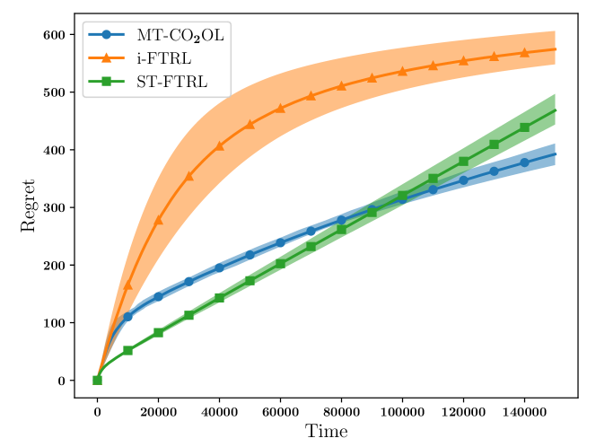
Figure 1: Multitask regret over time of MT-CO₂OL on a random communication graph with stochastic activations against two baselines: i-FTRL ($N$ independent instances of FTRL) and ST-FTRL (the multi-agent single-task algorithm of Cesa-Bianchi et al., (2020)).

We also prove a lower bound (Theorem 6) showing that our regret upper bounds are tight in some important special cases, such as regular communication graphs. Finally, we show that MT-CO₂OL can be made differentially private and prove that, for linear losses, privacy only degrades the multitask regret by a term logarithmic in $T$ (Theorem 8). This allows us to identify a privacy threshold above which sharing information no longer benefits the agents.

1.1 Related works

We review related works by focusing on multi-agent online learning with adversarial (nonstochastic) losses. In this area, we distinguish three main threads of research: single-task (or cooperative) learning, multitask (or heterogeneous) learning, and distributed optimization. We also distinguish between synchronous (all agents are active in each round) and asynchronous (one agent is active in each round) activation models. To the best of our knowledge, the study of cooperative online learning was initiated by Awerbuch and Kleinberg, (2008), who studied a cooperative-competitive synchronous bandit model in which agents are partitioned in unknown clusters and agents in the same cluster receive the same losses (i.e., solve a single-task problem) whereas the losses of agents in distinct clusters may be different.

Single-task. The synchronous bandit model was also studied by Cesa-Bianchi et al., (2019) and Bar-On and Mansour, (2019) in a network of agents where communication delays (based on the shortest-path distance) are taken into account. Their analysis was extended to linear bandits by Ito et al., (2020), and to linear semi-bandits by Della Vecchia and Cesari, (2021). Cesa-Bianchi et al., (2020) investigate the asynchronous online convex optimization setting without delays and where agents can only talk to their neighbors. Their analysis is extended to neighborhoods of higher order by Van der Hoeven et al., (2022), who also take communication delays into account. Hsieh et al., (2022) and Jiang et al., (2021) consider the same setting, but with a more abstract model of delays, not necessarily induced by shortest-path distance on a graph.

Multitask. One of the earliest contributions in the online multitask setting is by Cavallanti et al., (2010), who introduce an asynchronous multitask version of the Perceptron algorithm for binary classification. Murugesan et al., (2016) extend this to a model where task similarity is also learned. Another extension is considered by Cesa-Bianchi et al., (2022), who introduce a multitask version of Online Mirror Descent with arbitrary regularizers. See also Saha et al., (2011); Zhang et al., (2018); Li et al., (2019) for additional online multitask algorithms without performance bounds. Finally, Herbster et al., (2021) investigate an asynchronous bandit model on a social network in which the partition induced by the labeling assigning the best local action to each node has a small resistance-weighted cutsize.

Distributed online optimization. Yan et al., (2012) introduced a synchronous multitask setting where the comparator is the best global prediction for all tasks and the system’s performance is measured according to $\max_{j\in[N]}\sum_{i=1}^{N}\sum_{t=1}^{T}\ell_{t}^{i}\big{(}x_{t}^{j})$, where $\ell_{t}^{i}(x_{t}^{j})$ is the loss at time $t$ for the task of agent $i$ evaluated on the prediction at time $t$ of agent $j$. Crucially, at time $t$ each agent $j$ only observes $\nabla\ell_{t}^{j}(x_{t}^{j})$, and communication is used to gather information about other tasks. Hosseini et al., (2013) extended the analysis to general convex losses, moving beyond strongly convex ones. Yi and Vojnović, (2023) consider the bandit case, in which each agent observes the loss incurred rather than the gradient. Note that the synchronous bandit model of Cesa-Bianchi et al., (2019) is a special case of this setting (when $\ell_{t}^{1}=\ldots=\ell_{t}^{N}$ for all $t$). However, the regret scales with the independence number of the communication graph in Cesa-Bianchi et al., (2019), as opposed to spectral quantities such as the inverse of the spectral gap in distributed online optimization.

2 PROBLEM SETTING

In this section, we introduce the multitask online learning setting, and recall important existing results.

Setting.

Consider $N$ learning agents located at the nodes of a communication network described by an undirected graph $G=(V,E)$, where $V=[N]\coloneqq\{1,\ldots,N\}$. Let $\mathcal{N}_{i}=\{i\}\cup\{j\in[N]\,:\,(i,j)\in E\}$ be the neighbors of agent $i$ in $G$ (including $i$ itself), and $N_{i}=|\mathcal{N}_{i}|$. We denote $N_{\textnormal{min}}=\min_{i\in V}N_{i}$, and $N_{\textnormal{max}}=\max_{i\in V}N_{i}$. We assume that agents ignore the graph, but know the identity of their neighbors. Let $\mathcal{X}\subset\mathbb{R}^{d}$ be the agents common decision space, and $\ell_{1},\ell_{2},\ldots$ a sequence of convex losses from $\mathcal{X}$ to $\mathbb{R}$, secretly chosen by an oblivious adversary. The learning process is as follows. For $t=1,2,\ldots$

1. some agent $i_{t}\in[N]$ is activated

2. $i_{t}$ may fetch information from its neighbors $j\in\mathcal{N}_{i_{t}}$

3. $i_{t}$ predicts $x_{t}\in\mathcal{X}$

4. $i_{t}$ incurs the loss $\ell_{t}(x_{t})$ and observes $g_{t}\in\partial\ell_{t}(x_{t})$

5. $i_{t}$ may send information to its neighbors $j\in\mathcal{N}_{i_{t}}$ .

Communication is limited to steps 2 and 5, and only along edges incident on the active agent, hereby enforcing a decentralized learning process. As in distributed optimization algorithms (Hosseini et al.,, 2013), we use step 2 to fetch model-related information, and step 5 to send gradient-related information, see Sections 3 and 4. As shown in our analysis, both communication steps are key to obtain strong regret guarantees.

We measure performance through the multitask regret, defined as the sum of the agents’ individual regrets. The individual regret measures the performance of a single agent against the best decision in hindsight for its own personal task, i.e., for the sequence of losses associated to the time steps it is active. Namely, agent $i$ aims at minimizing for any $u^{(i)}\in\mathcal{X}$ its local regret $\sum_{t}\big{(}\ell_{t}(x_{t})-\ell_{t}(u^{(i)})\big{)}\,\mathbb{I}\{i_{t}=i\}$, and the global objective is thus to control for any $u^{(1)},\ldots,u^{(N)}\in\mathcal{X}$ the multitask regret $\sum_{i=1}^{N}\sum_{t=1}^{T}\big{(}\ell_{t}(x_{t})-\ell_{t}(u^{(i)})\big{)}\,\mathbb{I}\{i_{t}=i\}$ . Equivalently, this amounts to minimizing

$$\vspace{-0.15cm}R_{T}(U)=\sum_{t=1}^{T}\ell_{t}(x_{t})-\ell_{t}(U_{i_{t}:})$$ (1)

for any horizon $T$ and multitask comparator $U\in\mathcal{U}$, where $\mathcal{U}\coloneqq\big{\{}U\in\mathbb{R}^{N\times d}\colon U_{i:}\in\mathcal{X}\text{ for all }i\big{\}}$. Note that for simplicity in the rest of the paper we set $\mathcal{X}=\{x\in\mathbb{R}^{d}\colon\|x\|_{2}\leq 1\}$, and assume that all loss functions are $1$-Lipschitz, i.e., we have $\|g_{t}\|_{2}\leq 1$ for all $t$. Our analysis can be readily extended to any ball of generic radius $D$ and $L$-Lipschitz losses, up to scaling each regret bound by $DL$. As pointed out in the introduction, a naive approach to minimizing (1) consists in running $N$ independent instances of FTRL, without making use of steps 2 and 5. By Jensen’s inequality, such strategy satisfies for any $U\in\mathcal{U}$

$$R_{T}(U)=\sum_{i=1}^{N}2\sqrt{T_{i}}\leq 2\sqrt{NT}\,,$$ (2)

where $T_{i}=\sum_{t=1}^{T}\mathbb{I}\{i_{t}=i\}$. The purpose of this work is to introduce and analyze a new algorithm whose regret improves on (2) in terms of $N$. Our bounds should depend on the interplay between the task similarity and the structure of the communication graph.

Remark 1 (Comparison to Cesa-Bianchi et al., (2020)).

Although Cesa-Bianchi et al., (2020) also consider arbitrary communication graphs, their setting significantly differs from ours. Recall that they work in a single-task setting (where $u^{(1)}=u^{(2)}=\ldots=u^{(N)}$). Hence, their proof techniques are significantly different from ours. Moreover, while we only rely on gradient feedback, where the gradient is evaluated at the current prediction $x_{t}$, in their setting the learner is free to compute gradients at any point in the decision space. On the other hand, their communication model is restricted to sharing gradients while we can also fetch predictions.

Preliminaries.

Our algorithm builds upon MT-FTRL (Cesa-Bianchi et al.,, 2022), designed for the clique case. We recall important facts about this algorithm. MT-FTRL combines an instance of FTRL with a carefully chosen Mahalanobis regularizer and uses an adaptive learning rate based on Hedge—see Algorithm 1, where $G_{t}=e_{i_{t}}g_{t}^{\top}\in\mathbb{R}^{N\times d}$ denotes the gradient matrix full of $0$ except for row $i_{t}$ which contains $g_{t}$. The next result bounds the regret suffered by MT-FTRL.

Theorem 1 (Cesa-Bianchi et al., (2022, Theorem 9)).

Let $G$ be a clique. The regret of MT-FTRL with $\beta_{t-1}=\sqrt{t}$ satisfies for all $U\in\mathcal{U}$

$$R_{T}(U)\stackrel{{\scriptstyle\widetilde{\mathcal{O}}}}{{=}}\sqrt{1+\sigma^{2}(N-1)}\sqrt{T}\,,$$ (3)

where $\sigma^{2}=\sigma^{2}(U)=\frac{1}{N-1}\sum_{i=1}^{N}\big{\|}[U]_{i:}-\frac{1}{N}\sum_{j=1}^{N}[U]_{j:}\big{\|}_{2}^{2}$ is the comparator variance.

Requires: Number of agents $N$, learning rates $\beta_{t-1}$

Init: $A=(1+N)I_{N}-\bm{1}_{N}\bm{1}_{N}^{\top}$,   $\Xi=\{1/N,\,2/N,\ldots,1\}$,

        $p_{1}^{(\xi)}=\frac{1}{N}$  for all $\xi\in\Xi$

for $t=1,2,\ldots$ do

      

      for $\xi\in\Xi$ do

            

            // Set learning rate assuming $\sigma^{2}=\xi$

            

            $\eta^{(\xi)}_{t-1}=\frac{N}{\beta_{t-1}}\sqrt{1+\xi(N-1)}$

            // FTRL with Mahalanobis regularizer

             $\displaystyle X^{(\xi)}_{t}=\operatorname*{arg\,min}_{\begin{subarray}{c}X\in\mathcal{U}\\ \sigma^{2}(X)\leq\xi\end{subarray}}~{}\eta^{(\xi)}_{t-1}\left\langle\sum_{s\leq t-1}G_{s},X\right\rangle+\frac{1}{2}\|X\|_{A}^{2}$

      

      // Average the experts predictions

      

      Predict $X_{t}=\sum_{\xi\in\,\Xi}~{}p_{t}^{(\xi)}\,X_{t}^{(\xi)}$

      Incur linearized loss $\langle g_{t},[X_{t}]_{i_{t}:}\rangle$ and observe $g_{t}$

      // Update $p_{t}$ based on the experts losses

      

      for $\xi\in\Xi$ do

            

            $\displaystyle p_{t+1}^{(\xi)}=\frac{\exp\left(-\frac{\sqrt{\ln N}}{\beta_{t}}\sum_{s=1}^{t}\big{\langle}g_{s},[X_{s}^{(\xi)}]_{i_{s}:}\big{\rangle}\right)}{\sum_{k}\,\exp\left(-\frac{\sqrt{\ln N}}{\beta_{t}}\sum_{s=1}^{t}\big{\langle}g_{s},[X_{s}^{(k)}]_{i_{s}:}\big{\rangle}\right)}$

      

Algorithm 1  MT-FTRL (on linear losses)

Note that (3) is at most of the same order as the naive bound (2), as $\sigma^{2}(U)\leq 8$ for all $U$. On the other hand, (3) gets better as $\sigma^{2}$ decreases, i.e., as the tasks get similar, and recovers the single-agent bound $\sqrt{T}$ when $\sigma^{2}=0$, i.e., when all tasks are identical. Finally, we stress that MT-FTRL adapts to the true comparator variance $\sigma^{2}(U)$ without any prior knowledge about it.

The above approach crucially relies on the fact that the communication graph $G$ is a clique. In the next section, we show how to use MT-FTRL as a building block to devise an algorithm that can operate on any communication graph. Some of our bounds depend on notable parameters of the graph $G$, that we recall now.

Definition 1.

Let $G=(V,E)$. A subset $S\subset V$ is

• $k$-times independent in $G$ if the shortest path between any two vertices in $S$ is of length $k+1$. The cardinality of the largest $k$-times independent set of $G$ is denoted $\alpha_{k}(G)$. For $k=1$, we use the term independent set and adopt the notation $\alpha(G)$.

• dominating in $G$ if any vertex in $G\setminus S$ has a neighbor in $S$. The cardinality of the smallest dominating set of $G$ is denoted $\gamma(G)$ and called domination number of $G$.

It is well known that: $\alpha_{2}(G)\leq\gamma(G)\leq\alpha(G)\leq|V|$.

3 ALGORITHM AND ANALYSIS

Requires: Base algorithm AlgoClique, weights $w_{ij}$

for $t=1,2,\ldots$ do

      

      Active agent $i_{t}$

       fetches $\big{[}Y_{t}^{(j)}\big{]}_{i_{t}:}$ from each $j\in\mathcal{N}_{i_{t}}$

       predicts $x_{t}=\sum_{j\in\mathcal{N}_{i_{t}}}w_{i_{t}j}\big{[}Y_{t}^{(j)}\big{]}_{i_{t}:}$

       pays $\ell_{t}(x_{t})$ and observes $g_{t}\in\partial\ell_{t}(x_{t})$

       sends $\big{(}i_{t},w_{i_{t}j}\,g_{t}\big{)}$ to each $j\in\mathcal{N}_{i_{t}}$

      for $j\in\mathcal{N}_{i_{t}}$ do

            

            Agent $j$ feeds the linear loss $\langle w_{i_{t}j}\,g_{t},\cdot\,\rangle$ to their local instance of AlgoClique and obtains $Y^{(j)}_{t+1}$

      

Algorithm 2  MT-CO₂OL

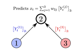
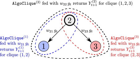
Figure 2: One Iteration of MT-CO₂OL. Active agent $2$ fetches their neighbor’s models and predicts with their weighted average $x_{t}$ (left). Then $2$ pays $\ell_{t}(x_{t})$, observes $g_{t}\in\partial\ell_{t}(x_{t})$, and sends back $w_{2j}\,g_{t}$. Finally, each local AlgoClique instance updates the models for the agents in the virtual clique centered on the agent running the instance (right).

In this section, we introduce and analyze MT-CO₂OL, a meta-algorithm for MultiTask COmmunication-COnstrained Online Learning. In particular, we prove two sets of regret upper bounds, depending on whether the agent activations are adversarial or stochastic. We also prove some lower bounds on the regret.

MT-CO₂OL uses as building block any multitask algorithm able to operate when the communication graph is a clique. In the following, we generically refer to this base algorithm as AlgoClique. MT-CO₂OL requires each agent $j\in V$ to run an instance of AlgoClique on a virtual clique over its neighbors $i\in\mathcal{N}_{j}$. The instance of AlgoClique run by $j$ maintains a matrix $Y_{t}^{(j)}\in\mathbb{R}^{N_{j}\times d}$, whose each row $\big{[}Y_{t}^{(j)}\big{]}_{i:}$ stores a model associated to task $i$, for any $i\in\mathcal{N}_{j}$. At time $t$, each $j\in\mathcal{N}_{i_{t}}$ sends to the active agent $i_{t}$ (or equivalently $i_{t}$ fetches from $j$) the model $\big{[}Y_{t}^{(j)}\big{]}_{i_{t}:}$. The prediction made by $i_{t}$ at time $t$ is the weighted average $x_{t}=\sum_{j\in\mathcal{N}_{i_{t}}}w_{i_{t}j}\big{[}Y_{t}^{(j)}\big{]}_{i_{t}:}$, where $w_{ij}$ are non-negative weights satisfying $\sum_{j\in\mathcal{N}_{i}}w_{ij}=1$. After predicting, $i_{t}$ observes $g_{t}\in\partial\ell_{t}(x_{t})$ and sends $w_{i_{t}j}\,g_{t}$ to each $j\in\mathcal{N}_{i_{t}}$. Agents $j\in\mathcal{N}_{i_{t}}$ then feed the linear loss $\langle w_{i_{t}j}g_{t},\cdot\rangle$ to their local instance of AlgoClique, obtaining the updated matrix $Y_{t+1}^{(j)}$. The pseudocode of MT-CO₂OL is summarized in Algorithm 2. See Figure 2 for an illustration of one iteration. Note that the local instance of AlgoClique run by agent $j$ does not have access to the global time $t$, e.g., to set the learning rate, but may only use the local time $\sum_{s\leq t}\mathbb{I}\left\{{i_{s}\in\mathcal{N}_{j}}\right\}$.

An important consequence of the fetch and send operations in MT-CO₂OL is that they enable running AlgoClique as if each agent $j$ were part of an isolated clique over $\mathcal{N}_{j}$, which in turn makes Theorem 1 applicable. Formally, let MT-CO₂OL be run over an arbitrary sequence $i_{1},\ldots,i_{T}$ of agent activations in a communication network $G=(V,E)$. Then, for each $j\in V$ and time $t$, the matrix $Y_{t}^{(j)}$ of models computed by AlgoClique run at node $j$ is identical to the matrix computed by AlgoClique run on a clique over $\mathcal{N}_{j}$ with the sequence of activations restricted to $\mathcal{N}_{j}$. This simple yet key observation allows us to derive the following lemma, which shows that the regret of MT-CO₂OL can be expressed in terms of the regrets suffered by AlgoClique run on the artificial cliques $\mathcal{N}_{j}$, for $j\in V$.

Lemma 2.

For any $U\in\mathbb{R}^{N\times d}$, let $U^{(j)}\in\mathbb{R}^{N_{j}\times d}$ be the matrix whose rows contain all $U_{i:}$ for $i$ in $\mathcal{N}_{j}$, sorted in ascending order of $i$. Furthermore, let $R^{\textnormal{clique-$j$}}_{T}$ be the regret suffered by AlgoClique run by agent $j$ on the linear losses $\langle w_{i_{t}j}\,g_{t},\cdot\rangle$ over the rounds $t\leq T$ such that $i_{t}\in\mathcal{N}_{j}$. Then, the regret of MT-CO₂OL satisfies

$$\forall\,U\in\mathbb{R}^{N\times d},\quad R_{T}(U)\leq\sum_{j=1}^{N}R^{\textnormal{clique-$j$}}_{T}\big{(}U^{(j)}\big{)}\,.$$

Proof.

Let $x_{1},\ldots,x_{T}$ be the predictions of MT-CO₂OL. By convexity of the $\ell_{t}$, we have

$$\sum_{t=1}^{T}\ell_{t}(x_{t})-\ell_{t}(U_{i_{t}:})\leq\sum_{t=1}^{T}\langle g_{t},x_{t}-U_{i_{t}:}\rangle$$ (4)

$$~{}~{}=\sum_{t=1}^{T}\sum_{i=1}^{N}\Big{\langle}g_{t},\sum_{j\in\mathcal{N}_{i}}w_{ij}\big{[}Y_{t}^{(j)}\big{]}_{i:}-U_{i:}\Big{\rangle}\mathbb{I}\left\{{i_{t}=i}\right\}$$

$$~{}~{}=\sum_{t=1}^{T}\sum_{i=1}^{N}\sum_{j\in\mathcal{N}_{i}}\left\langle g_{t},w_{ij}\left(\big{[}Y_{t}^{(j)}\big{]}_{i:}-U_{i:}\right)\right\rangle\mathbb{I}\left\{{i_{t}=i}\right\}$$

$$~{}~{}=\sum_{j=1}^{N}\sum_{t=1}^{T}\sum_{i\in\mathcal{N}_{j}}\left\langle w_{ij}\,g_{t},\big{[}Y_{t}^{(j)}\big{]}_{i:}-U_{i:}\right\rangle\mathbb{I}\left\{{i_{t}=i}\right\}$$ (5)

$$~{}~{}=\sum_{j=1}^{N}R^{\text{clique-$j$}}_{T}\big{(}U^{(j)}\big{)}\,,$$

where (5) follows from Lemma 9. ∎

Note that we could obtain similar guarantees by using the convexity of $\ell_{t}$ and postponing the linearization step (4) to the individual clique regrets. However, this would require computing the subgradients at the partial predictions $\big{[}Y_{t}^{(j)}\big{]}_{i:}$. Instead, MT-CO₂OL only uses the subgradient $g_{t}$ evaluated at the true prediction $x_{t}$. In the next section, we show how to leverage Lemma 2 to derive regret bounds for MT-CO₂OL.

3.1 Adversarial Activations

In this section, we assume the sequence $i_{1},i_{2},\ldots\in V$ of agent activations is chosen by an oblivious adversary. In the next theorem, we show that setting AlgoClique as MT-FTRL yields good regret bounds. Importantly, since the instance of MT-FTRL of agent $j$ is run on the virtual clique $\mathcal{N}_{j}$, the regret bound scales with the local task variances $\sigma^{2}_{j}=\frac{1}{2N_{j}(N_{j}-1)}\sum_{i,i^{\prime}\in\mathcal{N}_{j}}\big{\|}U_{i:}-U_{i^{\prime}:}\big{\|}_{2}^{2}$, quantifying how similar neighboring tasks are. Let $\sigma^{2}_{\textnormal{max}}=\max_{j\in[N]}\sigma^{2}_{j}$ and $\sigma^{2}_{\textnormal{min}}=\min_{j\in[N]}\sigma^{2}_{j}$. We are now ready to state our result.

Theorem 3.

Let $G=(V,E)$ be any communication graph. Consider MT-CO₂OL where the base algorithm AlgoClique run by each agent $j\in V$ is an instance of MT-FTRL with parameters $N=N_{j}$ and $\beta_{t-1}=\max_{i\in\mathcal{N}_{j}}w_{ij}\sqrt{1+\sum_{s\leq t-1}\mathbb{I}\left\{{i_{s}\in\mathcal{N}_{j}}\right\}}$. Then, the regret of MT-CO₂OL satisfies for all $U\in\mathcal{U}$

$$R_{T}(U)\stackrel{{\scriptstyle\widetilde{\mathcal{O}}}}{{=}}\sum_{j=1}^{N}\max_{i\in\mathcal{N}_{j}}w_{ij}\sqrt{1+\sigma_{j}^{2}(N_{j}-1)}\sqrt{\sum_{i\in\mathcal{N}_{j}}T_{i}}\,.$$

Setting $w_{ij}=\mathbb{I}\left\{{j\in\mathcal{N}_{i}}\right\}/N_{i}$ we obtain

$$R_{T}(U)\stackrel{{\scriptstyle\widetilde{\mathcal{O}}}}{{=}}\sqrt{1+\sigma_{\textnormal{max}}^{2}(N_{\textnormal{max}}-1)}\sqrt{\frac{NT}{\rho N_{\textnormal{min}}}}$$

where $\rho=N_{\textnormal{min}}/N_{\textnormal{max}}\leq 1$ measures how far $G$ is from being regular. Finally, there exist some $w_{ij}$ such that

$$R_{T}(U)\stackrel{{\scriptstyle\widetilde{\mathcal{O}}}}{{=}}\sqrt{1+\sigma_{\textnormal{max}}^{2}(N_{\textnormal{max}}-1)}\sqrt{\gamma(G)\,T}\,.$$

Theorem 3 provides three results with different flavors. The first bound is the most general, and holds for any choice of weights $w_{ij}$. It shows that the regret of MT-CO₂OL improves as the $\sigma_{j}^{2}$ get smaller, i.e., when neighbors in $G$ have similar tasks. The second bound uses uniform weights that only depend on local information (the neighborhood sizes). Interestingly, the bound depends on the total horizon $T$ instead of the individual $T_{i}$, and gets smaller when $G$ is dense ($N_{\textnormal{min}}\gg 1$) and nearly regular ($\rho\to 1)$, see Corollary 4. Finally, the third bound uses knowledge of the full graph $G$ (i.e., the domination number, which is NP-hard to compute) to set the weights. This bound can be viewed a multitask version of the single-task bound $\sqrt{\gamma(G)\,T}$ achieved by the centralized algorithm that pre-computes a dominating set and then requires each node to use and update only the model stored in its dominating node. This bound also shows that—lacking any global knowledge of the graph—sharing models and gradients is strictly better than sharing gradients only, as the latter method suffers from a lower bound of $\sqrt{\alpha(G)\,T}$ (Cesa-Bianchi et al.,, 2020). We now instantiate our bound for uniform weights to some special graphs.

Corollary 4.

Under the assumptions of Theorem 3, set $w_{ij}=\mathbb{I}\left\{{j\in\mathcal{N}_{i}}\right\}/N_{i}$. If $G$ is $K$-regular, then

$$R_{T}(U)\stackrel{{\scriptstyle\widetilde{\mathcal{O}}}}{{=}}\sqrt{1+K\,\sigma_{\textnormal{max}}^{2}}\,\sqrt{\frac{NT}{K+1}}\,.$$

If $G$ is a union of $\chi$ cliques, then

$$R_{T}(U)\stackrel{{\scriptstyle\widetilde{\mathcal{O}}}}{{=}}\sqrt{\chi+\sigma^{2}_{\textnormal{max}}(N-\chi)}\sqrt{T}\,.$$

The regret bound for $K$-regular graphs improves upon the $\sqrt{\alpha(G)\,T}$ bound proven by Cesa-Bianchi et al., (2020) in the more restrictive setting of single-task problems with stochastic activations. Indeed, by Turan’s theorem, see e.g., Mannor and Shamir, (2011, Lemma 3), we have that $N/(K+1)\leq\alpha(G)$ for $K$-regular graphs. This shows that the fetch step in MT-CO₂OL, which is missing in the learning protocol of Cesa-Bianchi et al., (2020), is key to derive improved regret guarantees. Regarding the second bound in Corollary 4, we recover the bound of MT-FTRL (Cesa-Bianchi et al.,, 2022) when $\chi=1$. Notably, MT-CO₂OL achieves these regret bounds without requiring knowledge of the graph structure.

3.2 Stochastic Activations

In this section, we show that MT-CO₂OL enjoys improved regret bounds when the agent activations are stochastic rather than adversarial. Formally, let $q_{1},\ldots,q_{N}\in[0,1]^{N}$ such that $\sum_{i=1}^{N}q_{i}=1$. Let $i_{1},\ldots,i_{T}$ be independent random variables denoting agent activations such that for every $t$ we have $\mathbb{P}(i_{t}=i)=q_{i}$. We also define $Q_{j}=\sum_{i\in\mathcal{N}_{j}}q_{i}$. In the following theorem, we show how MT-CO₂OL can adapt to the stochasticity to attain better regret bounds. For simplicity, we assume the algorithm discussed below has access to the conditional probabilities $q_{i}/Q_{j}$. In Remark 2, we discuss a simple strategy to extend the analysis to the case where only a lower bound on $\min_{i}q_{i}$ is available.

Theorem 5.

Let $G=(V,E)$ be any communication graph. Consider MT-CO₂OL where the base algorithm AlgoClique run by each agent $j\in V$ is an instance of MT-FTRL with parameters $N=N_{j}$ and $\beta_{t-1}=\sqrt{\sum_{i\in\mathcal{N}_{j}}\frac{q_{i}}{Q_{j}}\,w_{ij}^{2}}\sqrt{1+\sum_{s\leq t-1}\mathbb{I}\left\{{i_{s}\in\mathcal{N}_{j}}\right\}}$. Then, the regret of MT-CO₂OL satisfies for all $U\in\mathcal{U}$

$$\mathbb{E}[R_{T}(U)]\stackrel{{\scriptstyle\widetilde{\mathcal{O}}}}{{=}}\left(\sum_{j=1}^{N}\sqrt{\sum_{i\in\mathcal{N}_{j}}q_{i}\,w_{ij}^{2}}\sqrt{1+\sigma_{j}^{2}(N_{j}-1)}\right)\sqrt{T}\,,$$

where the expectation is taken over $i_{1},\ldots,i_{T}$. Setting $w_{ij}=q_{j}/Q_{i}$ we obtain

$$\mathbb{E}[R_{T}(U)]\stackrel{{\scriptstyle\widetilde{\mathcal{O}}}}{{=}}\sqrt{1+\sigma_{\textnormal{max}}^{2}(N_{\textnormal{max}}-1)}\sqrt{\alpha(G)\,T}\,.$$

The improvement with respect to Theorem 3 is a natural consequence of the stochastic activations. Indeed, the term $\max_{i\in\mathcal{N}_{j}}w_{ij}$ arises because agent $j$ receives scaled gradients from its neighbors $i\in\mathcal{N}_{j}$, with squared norms bounded by $\|w_{ij}\,g_{t}\|_{2}^{2}\leq\max_{i\in\mathcal{N}_{j}}w_{ij}^{2}$. With stochastic activations, this norm can be bounded in expectation by $\sum_{i\in\mathcal{N}_{j}}\frac{q_{i}}{Q_{j}}w_{ij}^{2}$, resulting in the improvement seen in in the first bound of Theorem 5. In the second bound, we show that an appropriate choice of weights $w_{ij}$ allows to recover the $\sqrt{\alpha(G)\,T}$ bound derived by Cesa-Bianchi et al., (2020) in the single-task setting ($\sigma_{\textnormal{max}}^{2}=0$). Importantly, the choice of $w_{ij}$ remains local to agent $j$, and does not require knowledge of the full communication graph. Finally, while Corollary 4 shows regret bounds sharper than $\sqrt{\alpha(G)\,T}$ in the more general adversarial case, those bounds only apply to particular graphs. In contrast, the results of Theorem 5 are valid for any graph. We conclude this section with a remark extending the guarantees to the case where the $q_{j}/Q_{i}$ have to be estimated.

Remark 2 (Extension to unknown $q_{i}$).

Both the choice of learning rates $\beta_{t-1}$ and weights $w_{ij}$ in the second claim of Theorem 5 require that agent $j$ can access the conditional probabilities $q_{i}/Q_{j}$. When the latter are unknown, they can be estimated easily through $\widehat{\pi}_{ij}(t)\coloneqq\sum_{s\leq t}\mathbb{I}\left\{{i_{s}=i}\right\}/\sum_{s\leq t}\mathbb{I}\left\{{i_{s}\in\mathcal{N}_{j}}\right\}$. In Section A.4, we show that the 2-step strategy consisting in first computing the $\widehat{\pi}_{ij}$ and then running MT-CO₂OL with $\widehat{\pi}_{ij}$ instead of $q_{i}/Q_{j}$ suffers minimal additional regret. Note that, although appealing, the idea of replacing $q_{i}/Q_{j}$ in $\beta_{t-1}$ by $\widehat{\pi}_{ij}(t)$ at each time step $t$ would not work, as it would disrupt the monotonicity of the learning rate sequence $\beta_{t-1}$.

3.3 Lower Bounds

We conclude the regret analysis by providing lower bounds. In particular, we show that MT-CO₂OL’s regret bound for regular graphs is tight up to constant factors.

Theorem 6.

Let $G$ be any communication graph. Then for any algorithm following Section 2’s protocol:

1. there exists a sequence of activations and gradients such that the algorithm suffers regret

   $$\sup_{U\in\mathcal{U}}R_{T}(U)\geq\frac{1}{3}\max\left\{\!\sqrt{1+\sigma^{2}(N-1)},\sqrt{\alpha_{2}(G)}\right\}\!\sqrt{T}.$$

2. for any even number $K$, there exists a $K$-regular graph and a sequence of activations and gradients such that the algorithm suffers regret

   $$\sup_{U\in\mathcal{U}}R_{T}(U)\geq\frac{1}{5}\sqrt{1+K\,\sigma^{2}_{\textnormal{min}}}\,\sqrt{\frac{NT}{K}}\,.$$

4 A PRIVATE VARIANT

MT-CO₂OL involves a gradient-sharing step, potentially harming privacy if losses contain sensitive information. In this section, we modify MT-CO₂OL so as to satisfy loss-level differential privacy. We prove that for linear losses, privacy only degrades the regret by a term logarithmic in $T$. Additionally, we establish privacy thresholds where sharing information becomes ineffective. Our analysis is based on the following privacy notion.

Definition 2.

We consider a randomized multi-agent algorithm $\mathcal{A}$, governing the communication between $N$ agents. Let $m^{(i)}_{t}$ denote the batch of messages sent by agent $i$ to the other agents at time $t$. For any $\varepsilon>0$, $\mathcal{A}$ is loss-level $\varepsilon$-differentially private (or $\varepsilon$-DP for short) if for all $i\in[N]$ and set $\mathcal{M}$ of sequences of messages

$$\frac{{\mathbb{P}}\big{(}m^{(i)}_{1},\ldots,m^{(i)}_{T}\in\mathcal{M}\mid i_{1},\ell_{1},\ldots,i_{T},\ell_{T}\big{)}}{{\mathbb{P}}\big{(}m^{(i)}_{1},\ldots,m^{(i)}_{T}\in\mathcal{M}\mid i_{1},\ell^{\prime}_{1},\ldots,i_{T},\ell^{\prime}_{T}\big{)}}\leq e^{\varepsilon}\,,$$ (6)

where $(\ell^{\prime}_{t})_{t\leq T}$ and $(\ell_{t})_{t\leq T}$ differ by at most one entry.

As it applies to messages between agents, our definition of DP is more general than traditional notions which focus on predictions, as commonly done in single-agent scenarios (Jain et al.,, 2012; Agarwal and Singh,, 2017). Note that a similar definition has been employed by Bellet et al., (2018), in the batch case though.

Our modification of MT-CO₂OL relies on the fact that MT-FTRL only requires information on sums of gradients and sums of inner products between predictions and gradients (for Hedge). This allows us to use aggregation trees (Dwork et al.,, 2010; Chan et al.,, 2011), enabling the DP release of cumulative vector sums so that the level of noise introduced remains logarithmic in the number of vectors. In particular, agent $i_{t}$ can compute:

• Sanitized versions $\widetilde{\gamma}^{(i)}_{t}$ of the sums of gradients observed by the agents $\sum_{s\leq t}g_{s}\,\mathbb{I}\left\{{i_{s}=i}\right\}$;

• Sanitized versions $\widetilde{s}_{t,i}^{(j,\xi)}$ of the sums of inner products between predictions of expert $\xi$ of agent $j$ and weighted gradients $\sum_{s\leq t-1}\langle w_{ij}g_{s},\big{[}X_{s}^{(j,\xi)}\big{]}_{i:}\rangle\mathbb{I}\left\{{i_{s}=i}\right\}$.

This technique was used in Guha Thakurta and Smith, (2013); Agarwal and Singh, (2017) for DP single-agent online learning. As in Agarwal and Singh, (2017), we use TreeBasedAgg, which tweaks the original tree-aggregation algorithm to obtain identically distributed noise across rounds.

Requires: Base algorithm DPMT-FTRL, weights $w_{ij}$, privacy level $\varepsilon$, distributions $\mathcal{D}_{d}$, $\mathcal{D}_{1}$

for $t=1,2,\ldots$ do

      

      Active agent $i_{t}$

       fetches $\big{[}Y_{t}^{(j)}\big{]}_{i_{t}:}$, $\Big{\{}\big{[}X_{t}^{(j,\xi)}\big{]}_{i_{t}:}\,:\xi\in\Xi_{j}\Big{\}}$ from each

       $j\in\mathcal{N}_{i_{t}}$

       predicts $x_{t}=\sum_{j\in\mathcal{N}_{i_{t}}}w_{i_{t}j}\big{[}Y_{t}^{(j)}\big{]}_{i_{t}:}$

       pays $\ell_{t}(x_{t})$ and observes $g_{t}\in\partial\ell_{t}(x_{t})$

       updates $\gamma_{t}^{(i_{t})}=\gamma_{t}^{(i_{t})}+g_{t}$

       computes $\widetilde{\gamma}_{t}^{(i_{t})}$ using an instance of

       TreeBasedAgg with distribution $\mathcal{D}_{d}$

      

      for $j\in\mathcal{N}_{i_{t}}$ do

            

            for $\xi\in\Xi_{j}$ do

                   $s_{t,i_{t}}^{(j,\xi)}=s_{t-1,i_{t}}^{(j,\xi)}+w_{i_{t}j}\big{\langle}[X_{t}^{(j,\xi)}]_{i_{t}:},g_{t}\big{\rangle},$

                  computes $\widetilde{s}_{t,i_{t}}^{(j,\xi)}$ using an instance of

                  TreeBasedAgg set with distribution $\mathcal{D}_{1}$

            sends $\big{(}i_{t},w_{i_{t}j}\,\widetilde{\gamma}_{t}^{(i_{t})},\{\widetilde{s}_{t,i_{t}}^{(j,\xi)}:\xi\in\Xi_{j}\}\big{)}$ to $j$

            Agent $j$ feeds $\big{(}w_{i_{t}j}\,\widetilde{\gamma}_{t}^{(i_{t})},\{\widetilde{s}_{t,i_{t}}^{(j,\xi)}:\xi\in\Xi_{j}\}\big{)}$ to their local instance of DPMT-FTRL and obtains $\big{(}Y^{(j)}_{t+1},\{X_{t+1}^{(j,\xi)},~{}\forall\xi\in\Xi_{j}\}\big{)}$.

      

Algorithm 3 DPMT-CO₂OL

The resulting algorithm, called DPMT-CO₂OL, is described in Algorithm 3. It invokes the $\varepsilon$-DP version of MT-FTRL, summarized in the supplementary material (Algorithm 4). We now prove that DPMT-CO₂OL is $\varepsilon$-DP.

Theorem 7.

Let $G$ be any graph, and for any $\varepsilon>0$, let $\varepsilon^{\prime}=\varepsilon/(6N_{\textnormal{max}}^{2})$. Assume that DPMT-CO₂OL is run on linear losses with $\mathcal{D}_{d}$ set to a $d$-dimensional Laplacian distribution with parameter $\frac{\sqrt{d}\ln T}{\varepsilon^{\prime}}$, and $\mathcal{D}_{1}$ set to a $1$-dimensional Laplacian distribution with parameter $\frac{\ln T}{\varepsilon^{\prime}}$. Then DPMT-CO₂OL is $\varepsilon$-DP.

Next, we state the regret bound for DPMT-CO₂OL with adversarial agent activations and linear losses.

Theorem 8.

Let $G=(V,E)$ be any communication graph, Consider DPMT-CO₂OL where the base algorithm run by each agent $j\in V$ is an instance of DPMT-FTRL with parameters $N=N_{j}$ and $\beta_{t-1}=\max_{i\in\mathcal{N}_{j}}w_{ij}\sqrt{1+\sum_{s\leq t-1}\mathbb{I}\left\{{i_{s}\in\mathcal{N}_{j}}\right\}}$. Then the regret of DPMT-CO₂OL run over linear losses with $\mathcal{D}_{d}$ and $\mathcal{D}_{1}$ set as in Theorem 7 satisfies

$$\mathbb{E}[R_{T}(U)] \stackrel{{\scriptstyle\widetilde{\mathcal{O}}}}{{=}}\sum_{j=1}^{N}\max_{i\in\mathcal{N}_{j}}w_{ij}\sqrt{1+\sigma_{j}^{2}(N_{j}-1)}\sqrt{\sum_{i\in\mathcal{N}_{j}}T_{i}}$$

$$~{}~{}~{}+\frac{dN_{\textnormal{max}}^{2}\ln^{2}T}{\varepsilon}\,\sum_{j=1}^{N}N_{j}^{2}\,,$$ (7)

where randomness is due to sanitization.

Note that the cost of privacy, i.e., the second line in bound (7), remains the same for stochastic activations.

Theorem 8 shows that using the private version of our algorithm results in an additional term in the regret which is only of order ${(\ln T)^{2}}/{\varepsilon}$. In particular, in the single-agent case ($N=1$) we recover the result of Agarwal and Singh, (2017). In the multi-agent case, the additional term due to privacy is negligible when $T\gg 1/{\varepsilon}$. However, the bound clearly shows that running DPMT-CO₂OL when $\varepsilon=\mathcal{O}\big{(}(\ln T)^{2}/T^{1/2+\beta}\big{)}$ for $\beta>0$ is worse than running $N$ instances of FTRL without communication, which gives a regret of order $\sqrt{NT}$. In short, if agents are too private, listening to neighbors introduces more noise than valuable information.

The assumption of linear losses is crucial for Theorem 7, as it ensures that predictions do not affect gradients. If losses are convex but not necessarily linear, we can still implement DPMT-CO₂OL by adding Laplacian noise of parameter $1/\varepsilon$ to each individual gradient. It can be shown that this method yields a total privacy cost of order $\sum_{j=1}^{N}\sqrt{\sum_{i\in\mathcal{N}_{j}}T_{i}}\big{/}{\varepsilon^{2}}$. In particular, in the case of a $K$-regular graph, the cut-off value for $\varepsilon$ below which sharing information is detrimental is $(N/K^{2})^{1/4}$ up to constant factors. This is much worse than the linear case, where this cut-off value vanishes as $T\to\infty$.

Interestingly, the proof of Theorem 8 also shows that knowing the task variances $\sigma_{j}^{2}$ reduces the cost of privacy, because the instances of MT-FTRL do not need to use experts to adapt to $\sigma_{j}^{2}$. In particular, the active agent can avoid sharing $\widetilde{s}_{t,i_{t}}^{(j,\xi)}$, which leads to a significant reduction in the information leakage. Then, the cost of privacy becomes of order $\Big{(}\sum_{j=1}^{N}\sqrt{N_{j}\big{(}1+\sigma_{j}^{2}(N_{j}-1)\big{)}}\Big{)}d\ln^{2}T/\varepsilon$.

5 EXPERIMENTS

In this section, we describe experiments supporting our theoretical claims. In our experiments, the communication graphs $G$ are generated using the Erdős–Rényi’s model: given $N=30$ vertices, the edge between two vertices is included in $G$ with probability $p=0.9$. Our results are averaged over $48$ independent draws of such graphs. The tasks are defined using square losses that are minimized at points given by the rows of a random matrix $U$. The matrix $U$ is drawn according to a centered Gaussian distribution with covariance matrix $(I_{N}+\lambda L_{G})^{-1}$, where $L_{G}$ is the Laplacian of the graph $G$. The local task variance is then controlled via the parameter $\lambda$, which in our experiments varies in the set $\{10^{10},10,9,8,7,6,5,4,3,2\}$. The average local task standard deviation $\bar{\sigma}$ resulting from these choices of $\lambda$ are the $x$-coordinates of points in Figure 3. Finally, activations are stochastically generated with $q_{i}=1/N$.

For practical reasons, the version of MT-CO₂OL used here slightly differs from Algorithm 2, as our adaptive part is based on the Krichevsky-Trofimov algorithm (see Algorithm 5 for details) to account for task variances and domain diameter. This variant has regret guarantees similar to the original MT-CO₂OL (see Appendix C) but is simpler to run in practice. It is however nontrivial to make it $\varepsilon$-DP, which is the reason why in the theoretical analysis we privileged Hedge over Krichevsky-Trofimov. We consider two baselines: the first one, i-FTRL, consists in running instances of FTRL on agents that do not communicate with each other. The second method, ST-FTRL, is the multi-agent single-task algorithm with communication graph $G$ introduced in (Cesa-Bianchi et al.,, 2020). Note that this algorithm requires oracle access to the loss function, instead of just access to the gradient computed at the current prediction. This represents a significant advantage. In particular, the regret guarantees for this algorithm only hold given access to the loss function oracle. To ensure fair comparisons, we extend adaptivity to the diameter to both i-FTRL and ST-FTRL using the Krichevsky-Trofimov method.

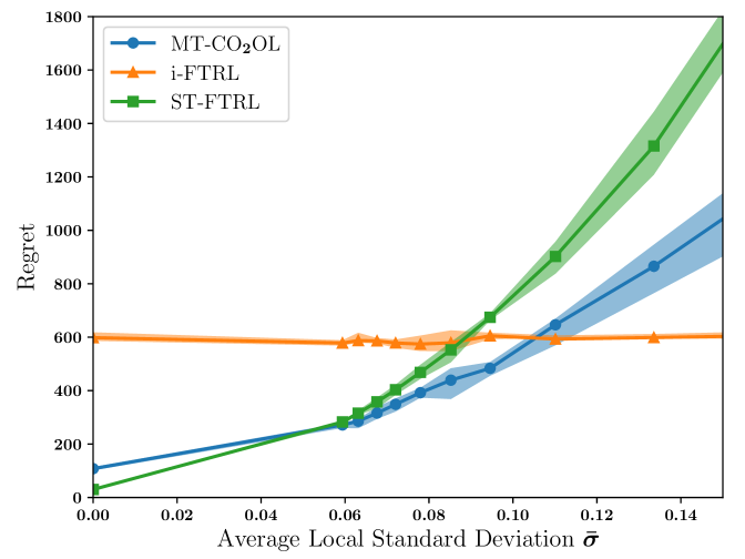
Figure 3: Multitask regret at horizon $T=150\,000$.

Figure 3 shows the (multitask) regret of these algorithms. As expected, the performance of i-FTRL is independent from $\bar{\sigma}$ and dominates when the latter is large (i.e., tasks are very different). On the other hand, ST-FTRL wins when $\bar{\sigma}$ is close to zero (i.e., tasks are very similar). Finally, MT-CO₂OL outperforms the baselines for intermediate values of $\bar{\sigma}$ (see also Figure 1 that plots the regret against time for $\bar{\sigma}=0.08$).

6 CONCLUSION

We introduced and analyze MT-CO₂OL, an algorithm tackling multitask online learning on arbitrary communication networks. Interesting generalizations of this work may focus on the cases where: (1) the communication network changes over time, (2) privacy levels are user-specific, (3) agents have further constraints (e.g., size-wise or frequency-wise) on the messages they send.

Appendix A Technical Proofs (Results from Section 3)

In this section, we gather the technical proofs of the results exposed in Section 3. We start by stating a lemma which allows to invert indices when summation is made over the edges of $G$. This result is in particular used to prove Lemma 2. We then prove all results stated in Section 3. Finally, we analyze an unsuccessful approach that runs $|E|$ instances of MT-FTRL that maintain predictions for all pair of agents $(i,j)$ such that $(i,j)\in E$.

Lemma 9.

Let $F\in\mathbb{R}^{N\times N}$ be any matrix (i.e., not necessarily symmetric). Then we have

$$\sum_{i=1}^{N}\sum_{j\in\mathcal{N}_{i}}F_{ij}=\sum_{j=1}^{N}\sum_{i\in\mathcal{N}_{j}}F_{ij}\,.$$

Proof.

We have

$$\sum_{i=1}^{N}\sum_{j\in\mathcal{N}_{i}}F_{ij}=\sum_{i=1}^{N}\sum_{j=1}^{N}F_{ij}~{}\mathbb{I}\left\{{j\in\mathcal{N}_{i}}\right\}=\sum_{i=1}^{N}\sum_{j=1}^{N}F_{ij}~{}\mathbb{I}\left\{{i\in\mathcal{N}_{j}}\right\}=\sum_{j=1}^{N}\sum_{i\in\mathcal{N}_{j}}F_{ij}\,.$$

∎

A.1 Proof of Theorem 3

See 3

Proof.

By Lemma 2, we have

$$R_{T}(U)\leq\sum_{j=1}^{N}R^{\textnormal{clique-$j$}}_{T}\big{(}U^{(j)}\big{)}\,,$$

where $R^{\textnormal{clique-$j$}}_{T}$ the regret suffered by MT-FTRL on the linear losses $\langle w_{i_{t}j}\,g_{t},\cdot\rangle$ over the rounds $t\leq T$ such that $i_{t}\in\mathcal{N}_{j}$. We now upper bound each of these terms individually. Let $j\in[N]$, using the notation in Algorithm 1 we have

$$R^{\textnormal{clique-$j$}}_{T}\big{(}U^{(j)}\big{)} =\sum_{t=1}^{T}\sum_{i\in\mathcal{N}_{j}}\left\langle w_{ij}\,g_{t},\big{[}Y_{t}^{(j)}\big{]}_{i:}-U^{(j)}_{i:}\right\rangle\mathbb{I}\left\{{i_{t}=i}\right\}$$

$$=\sum_{t\colon i_{t}\in\mathcal{N}_{j}}\left\langle w_{i_{t}j}\,g_{t},\big{[}Y_{t}^{(j)}\big{]}_{i_{t}:}-U^{(j)}_{i_{t}:}\right\rangle$$

$$=\sum_{t\colon i_{t}\in\mathcal{N}_{j}}\left\langle w_{i_{t}j}\,g_{t},\big{[}X_{t}\big{]}_{i_{t}:}-U^{(j)}_{i_{t}:}\right\rangle$$

$$\leq\underbrace{\sum_{t\colon i_{t}\in\mathcal{N}_{j}}\left\langle w_{i_{t}j}\,g_{t},\big{[}X_{t}\big{]}_{i_{t}:}-\big{[}X_{t}^{(\xi^{*})}\big{]}_{i_{t}:}\right\rangle}_{\text{Regret of {Hedge}}}+\underbrace{\sum_{t\colon i_{t}\in\mathcal{N}_{j}}\left\langle w_{i_{t}j}\,g_{t},\big{[}X_{t}^{(\xi^{*})}\big{]}_{i_{t}:}-U^{(j)}_{i_{t}:}\right\rangle}_{\text{Regret with choice $\xi^{*}$}}\,,$$ (8)

where $\xi^{*}=\operatorname*{arg\,min}_{\xi\in\,\Xi_{j}}\,\sum_{t\colon i_{t}\in\mathcal{N}_{j}}\Big{\langle}w_{i_{t}j}\,g_{t},\big{[}X_{t}^{(\xi)}\big{]}_{i_{t}:}\Big{\rangle}$. We start by upper bounding the regret due to Hedge. Let $\text{loss}_{t}\in\mathbb{R}^{N_{j}}$ be the vector storing the $w_{i_{t}j}\big{\langle}g_{t},\big{[}X_{t}^{(\xi)}\big{]}_{i_{t}:}\big{\rangle}$ for $\xi\in\Xi_{j}$, and $e^{*}\in\mathbb{R}^{N_{j}}$ the one-hot vector with an entry of $1$ at expert $\xi^{*}$. By the analysis of Hedge with regularizers $\psi_{t}(\bm{p})=\frac{\beta\sqrt{1+\sum_{s\leq t-1}\mathbb{I}\left\{{i_{s}\in\mathcal{N}_{j}}\right\}}}{\sqrt{\ln N_{j}}}\sum_{k=1}^{N_{j}}p_{k}\ln(p_{k})$, see e.g., Orabona, (2019, Section 7.5), we have

$$\sum_{t\colon i_{t}\in\mathcal{N}_{j}}\left\langle w_{i_{t}j}\,g_{t},\big{[}X_{t}\big{]}_{i_{t}:}-\big{[}X_{t}^{(\xi^{*})}\big{]}_{i_{t}:}\right\rangle =\sum_{t\colon i_{t}\in\mathcal{N}_{j}}\big{\langle}\,\text{loss}_{t},\bm{p}_{t}-e^{*}\big{\rangle}$$

$$\leq\beta\sqrt{\ln N_{j}\sum_{i\in\mathcal{N}_{j}}T_{i}}+\frac{\sqrt{\ln N_{j}}}{2\beta}\sum_{t\colon i_{t}\in\mathcal{N}_{j}}\frac{\|\text{loss}_{t}\|_{\infty}^{2}}{\sqrt{1+\sum_{s\leq t-1}\mathbb{I}\left\{{i_{s}\in\mathcal{N}_{j}}\right\}}}$$

$$\leq\beta\sqrt{\ln N_{j}\sum_{i\in\mathcal{N}_{j}}T_{i}}+\frac{\sqrt{\ln N_{j}}}{2\beta}\sum_{t\colon i_{t}\in\mathcal{N}_{j}}\frac{w_{i_{t}j}^{2}}{\sqrt{1+\sum_{s\leq t-1}\mathbb{I}\left\{{i_{s}\in\mathcal{N}_{j}}\right\}}}$$

$$\leq\sqrt{\ln N_{j}\sum_{i\in\mathcal{N}_{j}}T_{i}}\left(\beta+\frac{1}{\beta}\,\max_{i\in\mathcal{N}_{j}}w_{ij}^{2}\right)$$

$$=2\max_{i\in\mathcal{N}_{j}}w_{ij}\sqrt{\ln N_{j}\sum_{i\in\mathcal{N}_{j}}T_{i}}$$ (9)

if we choose $\beta=\max_{i\in\mathcal{N}_{j}}w_{ij}$. We now turn to the second regret. Assume first that $\sigma_{j}^{2}\leq 1$. Then, the regret with choice $\xi^{*}$ is in particular better than the regret with choice $\bar{\xi}\in\Xi_{j}$ such that $\bar{\xi}-\frac{1}{N_{j}}\leq\sigma_{j}^{2}\leq\bar{\xi}$. Recall that the sequence $X_{t}^{(\bar{\xi})}$ is generated by FTRL with the sequence of regularizers $\frac{1}{2}\|\cdot\|_{A_{j}}^{2}/\eta_{t-1}^{(\bar{\xi})}$. By the analysis of FTRL, see e.g., Orabona, (2019, Corollary 7.9), we have

$$\sum_{t\colon i_{t}\in\mathcal{N}_{j}}\Big{\langle}w_{i_{t}j}\,g_{t},\big{[} X_{t}^{(\bar{\xi})}\big{]}_{i_{t}:}-U^{(j)}_{i_{t}:}\Big{\rangle}$$

$$\leq\frac{\big{\|}U^{(j)}\big{\|}_{A_{j}}^{2}}{2\,\eta_{\sum_{i\in\mathcal{N}_{j}}T_{i}-1}^{(\bar{\xi})}}+\frac{1}{2}\sum_{t\colon i_{t}\in\mathcal{N}_{j}}\eta_{t-1}^{(\bar{\xi})}\big{\|}w_{i_{t}j}\,G_{t}\big{\|}_{A_{j}^{-1}}^{2}$$

$$\leq\frac{1+\sigma_{j}^{2}(N_{j}-1)}{2\sqrt{1+\bar{\xi}(N_{j}-1)}}~{}\max_{i\in\mathcal{N}_{j}}w_{ij}\sqrt{\sum_{i\in\mathcal{N}_{j}}T_{i}}+\frac{N\sqrt{1+\bar{\xi}(N_{j}-1)}}{2\max_{i\in\mathcal{N}_{j}}w_{ij}}\sum_{t\colon i_{t}\in\mathcal{N}_{j}}\frac{w_{i_{t}j}^{2}\,\big{[}A_{j}^{-1}\big{]}_{i_{t}i_{t}}\,\|g_{t}\|_{2}^{2}}{\sqrt{1+\sum_{s\leq t-1}\mathbb{I}\left\{{i_{s}\in\mathcal{N}_{j}}\right\}}}$$

$$\leq\frac{5}{2}\,\max_{i\in\mathcal{N}_{j}}w_{ij}\,\sqrt{1+\bar{\xi}(N_{j}-1)}\sqrt{\sum_{i\in\mathcal{N}_{j}}T_{i}}$$

$$\leq\frac{5}{2}\,\max_{i\in\mathcal{N}_{j}}w_{ij}\,\sqrt{1+\left(\sigma_{j}^{2}+\frac{1}{N_{j}}\right)(N_{j}-1)}\sqrt{\sum_{i\in\mathcal{N}_{j}}T_{i}}$$

$$\leq 4\,\max_{i\in\mathcal{N}_{j}}w_{ij}\,\sqrt{1+\sigma_{j}^{2}(N_{j}-1)}\sqrt{\sum_{i\in\mathcal{N}_{j}}T_{i}}\,.$$ (10)

Assume now that $\sigma_{j}^{2}\geq 1$. Then, the regret with choice $\xi^{*}$ is in particular better than the regret with choice $1$. The latter corresponds to independent learning (Cesa-Bianchi et al.,, 2022) and an analysis similar to the one above shows that its regret is bounded by

$$\max_{i\in\mathcal{N}_{j}}w_{ij}\,\sqrt{N_{j}\sum_{i\in\mathcal{N}_{j}}T_{i}}\leq\max_{i\in\mathcal{N}_{j}}w_{ij}\sqrt{1+\sigma_{j}^{2}(N_{j}-1)}\sqrt{\sum_{i\in\mathcal{N}_{j}}T_{i}}\,.$$ (11)

Substituting (9) and (10) or (11) (depending on the value of $\sigma_{j}^{2}$) into (8), we obtain

$$R_{T}(U)\leq 6\sum_{j=1}^{N}\max_{i\in\mathcal{N}_{j}}w_{ij}\left(\sqrt{1+\sigma_{j}^{2}(N_{j}-1)}+\ln N_{j}\right)\sqrt{\sum_{i\in\mathcal{N}_{j}}T_{i}}\,.$$

For the second claim, substituting $w_{ij}=\mathbb{I}\left\{{j\in\mathcal{N}_{i}}\right\}/N_{i}$ yields

$$\sum_{j=1}^{N}\max_{i\in\mathcal{N}_{j}}w_{ij}\sqrt{1+\sigma_{j}^{2}(N_{j}-1)}\sqrt{\sum_{i\in\mathcal{N}_{j}}T_{i}} =\sum_{j=1}^{N}\frac{\sqrt{1+\sigma_{j}^{2}(N_{j}-1)}}{\min_{i\in\mathcal{N}_{j}}N_{i}}\sqrt{\sum_{i\in\mathcal{N}_{j}}T_{i}}$$ (12)

$$\leq\frac{\sqrt{1+\sigma_{\textnormal{max}}^{2}(N_{\textnormal{max}}-1)}}{N_{\textnormal{min}}}\sum_{j=1}^{N}\sqrt{\sum_{i\in\mathcal{N}_{j}}T_{i}}$$

$$\leq\frac{\sqrt{1+\sigma_{\textnormal{max}}^{2}(N_{\textnormal{max}}-1)}}{N_{\textnormal{min}}}\sqrt{N\sum_{j=1}^{N}\sum_{i\in\mathcal{N}_{j}}T_{i}}$$

$$\leq\frac{\sqrt{1+\sigma_{\textnormal{max}}^{2}(N_{\textnormal{max}}-1)}}{N_{\textnormal{min}}}\sqrt{N\sum_{i=1}^{N}\sum_{j\in\mathcal{N}_{i}}T_{i}}$$

$$\leq\sqrt{1+\sigma_{\textnormal{max}}^{2}(N_{\textnormal{max}}-1)}\sqrt{\frac{NN_{\textnormal{max}}T}{N_{\textnormal{min}}^{2}}}\,,$$

where the second inequality comes from Jensen’s inequality and the third one from Lemma 9.

To prove the third claim, let $S_{\gamma}(G)$ be a smallest dominant set of $G$. For each $i\in[N]$, let $j(i)$ be the node in $\mathcal{N}_{i}$ that belongs to $S_{\gamma}(G)$ (if there are several, take the one with the smallest index). We set $w_{ij}=\delta_{jj(i)}$, i.e., agent $i$ completely delegates its prediction to its neighbour in the dominant set. Then, by Cauchy-Schwarz inequality we have

$$\sum_{j=1}^{N}\max_{i\in\mathcal{N}_{j}}w_{ij}\sqrt{1+\sigma_{j}^{2}(N_{j}-1)}\sqrt{\sum_{i\in\mathcal{N}_{j}}T_{i}} \leq\sqrt{1+\sigma_{\textnormal{max}}^{2}(N_{\textnormal{max}}-1)}\,\sum_{j\in S_{\gamma}(G)}\sqrt{\sum_{i\colon j(i)=j}T_{i}}$$

$$\leq\sqrt{1+\sigma_{\textnormal{max}}^{2}(N_{\textnormal{max}}-1)}\,\sqrt{\big{|}S_{\gamma}(G)\big{|}\sum_{j\in S_{\gamma}(G)}~{}\sum_{i\colon j(i)=j}T_{i}}$$

$$\leq\sqrt{1+\sigma_{\textnormal{max}}^{2}(N_{\textnormal{max}}-1)}\,\sqrt{\gamma(G)\,T}\,.$$

∎

A.2 Proof of Corollary 4

See 4

Proof.

The first claim of Corollary 4 is proved by using the last claim of Theorem 3, and recalling that for a $K$-regular graph we have $N_{\textnormal{max}}=N_{\textnormal{min}}=K+1$. Consider now a collection of $\chi$ cliques, $C_{1},\ldots,C_{\chi}$. Starting from the right-hand side of Equation 12, we have

$$\sum_{j=1}^{N}\frac{\sqrt{1+\sigma_{j}^{2}(N_{j}-1)}}{\max_{i\in\mathcal{N}_{j}}N_{i}}\sqrt{\sum_{i\in\mathcal{N}_{j}}T_{i}} =\sum_{k=1}^{\chi}\sum_{j\in C_{k}}\frac{\sqrt{1+\sigma_{j}^{2}(|C_{k}|-1)}}{|C_{k}|}\sqrt{\sum_{i\in C_{k}}T_{i}}$$

$$=\sum_{k=1}^{\chi}\sqrt{1+\sigma_{\textnormal{max}}^{2}(|C_{k}|-1)}\sqrt{\sum_{i\in C_{k}}T_{i}}$$

$$\leq\sqrt{\sum_{k=1}^{\chi}\big{(}1+\sigma_{\textnormal{max}}^{2}(|C_{k}|-1)\big{)}}~{}\sqrt{\sum_{k=1}^{\chi}\sum_{i\in C_{k}}T_{i}}$$

$$=\sqrt{\chi+\sigma_{\textnormal{max}}^{2}(N-\chi)}\,\sqrt{T}\,.$$

∎

A.3 Proof of Theorem 5

See 5

Proof.

The proof follows that of Theorem 3 until the decomposition of Equation 8. The analysis of Hedge with regularizers $\psi_{t}(\bm{p})=\frac{\beta\sqrt{1+\sum_{s\leq t-1}\mathbb{I}\left\{{i_{s}\in\mathcal{N}_{j}}\right\}}}{\sqrt{\ln N_{j}}}\sum_{k=1}^{N_{j}}p_{k}\ln(p_{k})$ then gives

$$\sum_{t\colon i_{t}\in\mathcal{N}_{j}}\left\langle w_{i_{t}j}\,g_{t},\big{[}X_{t}\big{]}_{i_{t}:}-\big{[}X_{t}^{(\xi^{*})}\big{]}_{i_{t}:}\right\rangle =\sum_{t\colon i_{t}\in\mathcal{N}_{j}}\big{\langle}\,\text{loss}_{t},\bm{p}_{t}-e^{*}\big{\rangle}$$

$$\leq\beta\sqrt{\ln N_{j}\sum_{i\in\mathcal{N}_{j}}T_{i}}+\frac{\sqrt{\ln N_{j}}}{2\beta}\sum_{t\colon i_{t}\in\mathcal{N}_{j}}\frac{\|\text{loss}_{t}\|_{\infty}^{2}}{\sqrt{1+\sum_{s\leq t-1}\mathbb{I}\left\{{i_{s}\in\mathcal{N}_{j}}\right\}}}$$

$$\leq\beta\sqrt{\ln N_{j}\sum_{i\in\mathcal{N}_{j}}T_{i}}+\frac{\sqrt{\ln N_{j}}}{2\beta}\sum_{t=1}^{T}\frac{w_{i_{t}j}^{2}\,\mathbb{I}\left\{{i_{t}\in\mathcal{N}_{j}}\right\}}{\sqrt{1+\sum_{s\leq t-1}\mathbb{I}\left\{{i_{s}\in\mathcal{N}_{j}}\right\}}}\,.$$ (13)

Taking expectation on both sides, we obtain

$$\mathbb{E}\left[\rule{0.0pt}{19.91684pt}\right.\sum_{t\colon i_{t}\in\mathcal{N}_{j}}\Big{\langle} w_{i_{t}j}\,g_{t},\big{[}X_{t}\big{]}_{i_{t}:}-\big{[}X_{t}^{(\xi^{*})}\big{]}_{i_{t}:}\Big{\rangle}\left.\rule{0.0pt}{19.91684pt}\right]$$

$$\leq\mathbb{E}\left[\beta\sqrt{\ln N_{j}\sum_{i\in\mathcal{N}_{j}}T_{i}}+\frac{\sqrt{\ln N_{j}}}{2\beta}\sum_{t=1}^{T}\frac{w_{i_{t}j}^{2}\,\mathbb{I}\left\{{i_{t}\in\mathcal{N}_{j}}\right\}}{\sqrt{1+\sum_{s\leq t-1}\mathbb{I}\left\{{i_{s}\in\mathcal{N}_{j}}\right\}}}\right]$$

$$\leq\beta\sqrt{\ln N_{j}~{}\mathbb{E}\left[\sum_{i\in\mathcal{N}_{j}}T_{i}\right]}+\frac{\sqrt{\ln N_{j}}}{2\beta}\mathbb{E}\left[\sum_{t=1}^{T}\mathbb{E}\left[\frac{w_{i_{t}j}^{2}\,\mathbb{I}\left\{{i_{t}\in\mathcal{N}_{j}}\right\}}{\sqrt{1+\sum_{s\leq t-1}\mathbb{I}\left\{{i_{s}\in\mathcal{N}_{j}}\right\}}}\,\bigg{|}\,i_{1},\ldots,i_{t-1},i_{t}\in\mathcal{N}_{j}\right]\right]$$

$$\leq\beta\sqrt{Q_{j}T\,\ln N_{j}}+\frac{\sqrt{\ln N_{j}}}{2\beta}\sum_{i\in\mathcal{N}_{j}}\frac{q_{i}}{Q_{j}}\omega^{2}_{ij}~{}\mathbb{E}\left[\sum_{t=1}^{T}\frac{\mathbb{I}\left\{{i_{t}\in\mathcal{N}_{j}}\right\}}{\sqrt{1+\sum_{s\leq t-1}\mathbb{I}\left\{{i_{s}\in\mathcal{N}_{j}}\right\}}}\right]$$

$$\leq\beta\sqrt{Q_{j}T\,\ln N_{j}}+\frac{\sqrt{\ln N_{j}}}{\beta}\sum_{i\in\mathcal{N}_{j}}\frac{q_{i}}{Q_{j}}\omega^{2}_{ij}~{}\mathbb{E}\left[\sqrt{\sum_{i\in\mathcal{N}_{j}}T_{i}}\right]$$

$$\leq 2\sqrt{\sum_{i\in\mathcal{N}_{j}}q_{i}\,w_{ij}^{2}}\sqrt{T\,\ln N_{j}}$$

if we choose $\beta=\sqrt{\sum_{i\in\mathcal{N}_{j}}\frac{q_{i}}{Q_{j}}w_{ij}^{2}}$. Note that the same analysis can be applied to the second regret in the decomposition of Equation 8. Overall, we obtain that for all $U\in\mathcal{U}$ we have

$$\mathbb{E}[R_{T}(U)]\leq 6\left(\sum_{j=1}^{N}\sqrt{\sum_{i\in\mathcal{N}_{j}}q_{i}\,w_{ij}^{2}}\sqrt{1+\sigma_{j}^{2}(N_{j}-1)}\right)\sqrt{T\ln N}\,.$$

To prove the second claim, substitute $w_{ij}=q_{j}/Q_{i}$ in the above equation and observe that

$$\sum_{j=1}^{N}\sqrt{\sum_{i\in\mathcal{N}_{j}}q_{i}\,w_{ij}^{2}} =\sum_{j=1}^{N}\sqrt{\sum_{i\in\mathcal{N}_{j}}\frac{q_{i}q_{j}^{2}}{Q_{i}^{2}}}=\sum_{j=1}^{N}q_{j}\sqrt{\sum_{i\in\mathcal{N}_{j}}\frac{q_{i}}{Q_{i}^{2}}}$$

$$\leq\sqrt{\sum_{j=1}^{N}q_{j}\sum_{i\in\mathcal{N}_{j}}\frac{q_{i}}{Q_{i}^{2}}}=\sqrt{\sum_{i=1}^{N}\sum_{j\in\mathcal{N}_{i}}q_{j}\frac{q_{i}}{Q_{i}^{2}}}=\sqrt{\sum_{i=1}^{N}\frac{q_{i}}{Q_{i}}}\leq\sqrt{\alpha(G)}\,,$$

where the first inequality comes from Jensen’s inequality, and the second one from a known combinatorial result, see e.g., Griggs, (1983) or Cesa-Bianchi et al., (2020, Lemma 3). ∎

A.4 Extension of Theorem 5 to unknown $q_{i}$

Theorem 10.

Let $G$ be any graph, and assume that the agent activations are stochastic. Consider the following strategy, run independently by each agent $j$ for its artificial clique, and based on its local time. First, predict $Y_{t}^{(j)}=0$ until the local time reaches $\tau\coloneqq\left\lceil\frac{4}{q_{\textnormal{min}}}\ln\big{(}2N^{2}T\big{)}\right\rceil$, where $q_{\textnormal{min}}=\min_{i\in[N]}q_{i}$. Then, predict $Y_{t}^{(j)}$ using MT-FTRL, run with $N=N_{j}$ and $\beta_{t-1}=\sqrt{\sum_{i\in\mathcal{N}_{j}}\widehat{\pi}_{ij}(\tau)\,w_{ij}^{2}}\sqrt{1+\sum_{s\leq t-1}\mathbb{I}\left\{{i_{s}\in\mathcal{N}_{j}}\right\}-\tau}$, where the $\widehat{\pi}_{ij}(\tau)$ are the empirical estimates of the $q_{i}/Q_{j}$ computed at local time $\tau$. Then, the regret satisfies for all $U\in\mathcal{U}$

$$\mathbb{E}[R_{T}(U)]\stackrel{{\scriptstyle\widetilde{\mathcal{O}}}}{{=}}\left(\sum_{j=1}^{N}\sqrt{\sum_{i\in\mathcal{N}_{j}}q_{i}\,w_{ij}^{2}}\sqrt{1+\sigma_{j}^{2}(N_{j}-1)}\right)\sqrt{T}+\frac{N}{q_{\textnormal{min}}}\,,$$

where the expectation is taken with respect to the agent activations, and $\widetilde{\mathcal{O}}$ neglects logarithmic terms in $N$ and $T$.

Proof.

We first introduce some notation. For any $j\in[N]$, $i\in\mathcal{N}_{j}$, and $t>0$, let $t^{(j)}=\sum_{s\leq t}\mathbb{I}\left\{{i_{s}\in\mathcal{N}_{j}}\right\}$ be the local time for the artificial clique centered at agent $j$, $\pi_{ij}=q_{i}/Q_{j}$, and $\widehat{\pi}_{ij}(t^{(j)})=\sum_{s\leq t}\mathbb{I}\left\{{i_{s}=i}\right\}/\sum_{s\leq t}\mathbb{I}\left\{{i_{s}\in\mathcal{N}_{j}}\right\}=\sum_{s\leq t}\mathbb{I}\left\{{i_{s}=i}\right\}/t^{(j)}$ be its natural estimator at local time $t^{(j)}$. The strategy is as follows. First, each agent $j$ predicts with $Y_{t}^{(j)}=0$ until its local time $t^{(j)}$ reaches some value $\tau_{j}$ to be determined later. It then builds the estimates $\widehat{\pi}_{ij}(\tau_{j})$ of the $\pi_{ij}$. Finally, from local time $\tau_{j}$ agent $j$ predicts $Y_{t}^{(j)}$ using its local instance of MT-FTRL, run with $N=N_{j}$, and $\beta_{t-1}=\sqrt{\sum_{i\in\mathcal{N}_{j}}\widehat{\pi}_{ij}(\tau_{j})\,w_{ij}^{2}}\sqrt{1+\sum_{s\leq t-1}\mathbb{I}\left\{{i_{s}\in\mathcal{N}_{j}}\right\}-\tau_{j}}$. We refer to this algorithm as MT-FTRL-Ada$q$.

Note that Lemma 2 still applies, such that we may only focus on the regret on the different instances of MT-FTRL-Ada$q$ run by the different agents. We differentiate two cases, depending on whether the event

$$\mathcal{E}\coloneqq\left\{\frac{\pi_{ij}}{2}\leq\widehat{\pi}_{ij}(\tau_{j})\leq\frac{3}{2}\pi_{ij}\,,\quad\forall j\in[N],\forall i\in\mathcal{N}_{j}\right\}$$

occurs or not. If $\mathcal{E}$ is not satisfied, the regret of the instance of MT-FTRL-Ada$q$ run by agent $j$ is trivially bounded by $T_{j}$, and that of the global approach by $T$. When $\mathcal{E}$ is satisfied, we can control the regret of the instance of MT-FTRL-Ada$q$ run by agent $j$ as follows. On the first $\tau_{j}$ round, the regret is bounded by $\tau_{j}$. From time step $\tau_{j}$ onward, we have $\frac{\pi_{ij}}{2}\leq\widehat{\pi}_{ij}(\tau_{j})\leq\frac{3}{2}\pi_{ij}$ and taking expectations on (13), with $\beta=\sqrt{\sum_{i\in\mathcal{N}_{j}}\widehat{\pi}_{ij}(\tau_{j})\,w_{ij}^{2}}$, we obtain, conditionally on $\mathcal{E}$

$$\mathbb{E}\left[\rule{0.0pt}{28.45274pt}\right.\sum_{\begin{subarray}{c}t\colon t^{(j)}\geq\tau_{j}+1\\ t\colon i_{t}\in\mathcal{N}_{j}\end{subarray}}\Big{\langle}w_{i_{t}j}\,g_{t},\big{[}X_{t}\big{]}_{i_{t}:}-\big{[}X_{t}^{(\xi^{*})}\big{]}_{i_{t}:}\Big{\rangle}~{}\bigg{|}~{}\mathcal{E}\left.\rule{0.0pt}{28.45274pt}\right]$$

$$\leq\mathbb{E}\left[\rule{0.0pt}{28.45274pt}\right.\sqrt{\sum_{i\in\mathcal{N}_{j}}\widehat{\pi}_{ij}(\tau_{j})\,w_{ij}^{2}}\sqrt{\ln N_{j}\sum_{t\colon t^{(j)}\geq\tau_{j}+1}\mathbb{I}\left\{{i_{t}\in\mathcal{N}_{j}}\right\}}$$

$$\hskip 34.14322pt+\frac{\sqrt{\ln N_{j}}}{2\sqrt{\sum_{i\in\mathcal{N}_{j}}\widehat{\pi}_{ij}(\tau_{j})\,w_{ij}^{2}}}\sum_{t\colon t^{(j)}=\tau_{j}+1}\frac{w_{i_{t}j}^{2}\,\mathbb{I}\left\{{i_{t}\in\mathcal{N}_{j}}\right\}}{\sqrt{1+\sum_{\begin{subarray}{c}s\colon s^{(j)}\geq\tau_{j}+1\\ s\leq t-1\end{subarray}}\mathbb{I}\left\{{i_{s}\in\mathcal{N}_{j}}\right\}}}~{}\bigg{|}~{}\mathcal{E}\left.\rule{0.0pt}{28.45274pt}\right]$$

$$\leq\mathbb{E}\left[\sqrt{\frac{3}{2}}\sqrt{\sum_{i\in\mathcal{N}_{j}}\pi_{ij}\,w_{ij}^{2}}\sqrt{\ln N_{j}\sum_{t\geq 1}\mathbb{I}\left\{{i_{t}\in\mathcal{N}_{j}}\right\}}+\frac{\sqrt{2}\sqrt{\ln N_{j}}}{2\sqrt{\sum_{i\in\mathcal{N}_{j}}\pi_{ij}\,w_{ij}^{2}}}\sum_{t=1}^{T}\frac{w_{i_{t}j}^{2}\,\mathbb{I}\left\{{i_{t}\in\mathcal{N}_{j}}\right\}}{\sqrt{1+\sum_{s\leq t-1}\mathbb{I}\left\{{i_{s}\in\mathcal{N}_{j}}\right\}}}\right]$$

$$\leq 2\sqrt{2}\sqrt{\sum_{i\in\mathcal{N}_{j}}q_{i}\,w_{ij}^{2}}\,\sqrt{T\,\ln N_{j}}\,.$$

The same method applies to the regret with choice $\xi^{*}$, see decomposition (8), and we finally obtain that the expected regret of the overall approach, is bounded by

$$\underbrace{\sum_{j=1}^{N}\tau_{j}}_{\coloneqq\tau}+\underbrace{9\left(\sum_{j=1}^{N}\sqrt{\sum_{i\in\mathcal{N}_{j}}q_{i}\,w_{ij}^{2}}\sqrt{1+\sigma_{j}^{2}(N_{j}-1)}\right)\sqrt{T\,\ln N}}_{\coloneqq\mathfrak{A}}\,,$$

conditionally to $\mathcal{E}$. Hence, we have

$$\mathbb{E}[R_{T}(U)]\leq\mathbb{E}\big{[}\mathbb{P}(\mathcal{E})(\tau+\mathfrak{A})+\mathbb{P}(\mathcal{E}^{\mathsf{c}})T\big{]}\leq\tau+\mathfrak{A}+\mathbb{E}\big{[}\mathbb{P}(\mathcal{E}^{\mathsf{c}})\big{]}T\,.$$ (14)

We now upper bound $\mathbb{P}(\mathcal{E}^{\mathsf{c}})$. Let $q_{\textnormal{min}}=\min_{i\in[N]}q_{i}$. For any $j\in[N]$ and $i\in\mathcal{N}_{j}$, by the multiplicative Chernoff bound (Mitzenmacher and Upfal,, 2005, Corollary 4.6) we have

$$\mathbb{P}\left(\widehat{\pi}_{ij}(\tau_{j})\leq\frac{\pi_{ij}}{2}\text{ or }\widehat{\pi}_{ij}(\tau_{j})\geq\frac{3}{2}\pi_{ij}\right)=\mathbb{P}\left(|\widehat{\pi}_{ij}(\tau_{j})-\pi_{ij}|\geq\frac{\pi_{ij}}{2}\right)\leq\exp\left({-\frac{\pi_{ij}}{12}\,\tau_{j}}\right)\leq\exp\left({-\frac{q_{\textnormal{min}}}{12}\,\tau_{j}}\right)\,,$$

and by the union bound

$$\mathbb{P}(\mathcal{E}^{\mathsf{c}})\leq N\sum_{j=1}^{N}\exp\left(-\frac{q_{\textnormal{min}}}{12}\,\tau_{j}\right)\,.$$ (15)

Substituting (15) into (14), and setting $\tau_{j}=\left\lceil\frac{12}{q_{\textnormal{min}}}\ln\big{(}2N^{2}T\big{)}\right\rceil$ for all $j$, we get

$$\mathbb{E}[R_{T}(U)] \leq\mathfrak{A}+\tau+2NT\sum_{j=1}^{N}\exp\left(-\frac{q_{\textnormal{min}}}{12}\,\tau_{j}\right)$$

$$\leq 9\left(\sum_{j=1}^{N}\sqrt{\sum_{i\in\mathcal{N}_{j}}q_{i}\,w_{ij}^{2}}\sqrt{1+\sigma_{j}^{2}(N_{j}-1)}\right)\sqrt{T\,\ln N}+\frac{12N}{q_{\textnormal{min}}}\ln\big{(}2N^{2}T\big{)}+N+1$$

$$\leq 9\left(\sum_{j=1}^{N}\sqrt{\sum_{i\in\mathcal{N}_{j}}q_{i}\,w_{ij}^{2}}\sqrt{1+\sigma_{j}^{2}(N_{j}-1)}\right)\sqrt{T\,\ln N}+\frac{14N}{q_{\textnormal{min}}}\ln\big{(}2N^{2}T\big{)}\,.$$

∎

A.5 Proof of Theorem 6

See 6

Proof.

Figure 4: Activated nodes in a $2$-regular graph.

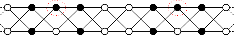
Figure 5: Activated nodes in a $4$-regular graph.

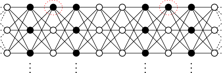
Figure 6: Activated nodes in a $6$-regular graph and more.

The first part of the lower bound is proved in (Cesa-Bianchi et al.,, 2022, Proposition 4). It establishes the existence of a comparator $U$ and a sequence of activations and gradients such that for any algorithm we have

$$R_{T}(U)\geq\frac{\sqrt{2}}{4}\sqrt{1+\sigma^{2}(N-1)}\sqrt{T}\,.$$ (16)

Note that this lower bound is oblivious to the communication graph $G$, and applies in particular to algorithms that follow the protocol described in Section 2 (where information can only be exchanged along the edges of $G$). For the second part of the first lower bound, let $S_{\alpha_{2}}(G)=\{j_{1},\ldots,j_{\alpha_{2}}\}$ be a largest twice independent set of $G$. Due to the communication protocol, it is immediate to check that if only nodes in $S_{\alpha_{2}}(G)$ are activated, then no information from an active node can be transmitted to another active node. Hence, the regret incurred by the nodes in $S_{\alpha_{2}}(G)$ are independent. Now, we know from standard online learning lower bounds that there exists some $u_{0}\in\mathbb{R}^{d}$ and a sequence $g_{1},\ldots,g_{T}$ such that the regret of a single agent is lower bounded by $\sqrt{T}/2$, see e.g., (Orabona,, 2019, Theorem 5.1). Let $U=(u_{0},\ldots,u_{0})\in\mathbb{R}^{N\times d}$, the activations be $j_{1}$ for the first $T/\alpha_{2}(G)$ steps, $j_{2}$ for the next $T/\alpha_{2}(G)$, and so on. Finally, consider the sequence of gradients $g_{1}\ldots g_{T/\alpha_{2}(G)}$ repeated $\alpha_{2}(G)$ times. In words, each agent in $S_{\alpha_{2}}(G)$ is sequentially given $g_{1}\ldots g_{T/\alpha_{2}(G)}$ and comparator $u_{0}$. Then the multitask regret satisfies

$$R_{T}(U)=\sum_{j\in S_{\alpha_{2}}(G)}R_{T/\alpha_{2}(G)}^{\textnormal{agent $j$}}\geq\sum_{j\in S_{\alpha_{2}}(G)}\frac{\sqrt{T/\alpha_{2}(G)}}{2}=\frac{\sqrt{\alpha_{2}(G)\,T}}{2}\,,$$ (17)

where the first equality comes from the independence due to the communication constraints, and the inequality from the single-task lower bound. Gathering (16) and (17) yields the desired result.

Consider now the special case of $K$-regular graphs. Figures 6, 6 and 6 show examples of communication graph on which our second lower bound can be attained. The idea is similar to that of the first lower bound. Only groups of nodes that are $2$-nodes apart (the black nodes in Figures 6, 6 and 6) are activated. This way, the regret incurred by the different groups are summed, as they are independent. On a group of nodes, one can identify a “central node” (circled with red dashes). We denote the set of indices of such nodes $\mathcal{J}_{\textnormal{cn}}$. By the multitask lower bound of Cesa-Bianchi et al., (2022), we know that for the (artificial) clique with center node $j$ there exists a comparator $U^{(j)}\in\mathbb{R}^{N_{j}\times d}$ and a sequence of activations and gradients such that we have a lower bound of order $\sqrt{1+K\,\sigma_{j}^{2}}\sqrt{\sum_{i\in\mathcal{N}_{j}}T_{i}}$. Overall by feeding these gradients to each groups of nodes, each activated $T/|\mathcal{J}_{\textnormal{cn}}|$ times, we obtain

$$R_{T}(U)=\sum_{j\in\mathcal{J}_{\textnormal{cn}}}R_{T/|\mathcal{J}_{\textnormal{cn}}|}^{\textnormal{group centered at $j$}}(U^{(j)})\geq\frac{\sqrt{2}}{4}\sum_{j\in\mathcal{J}_{\textnormal{cn}}}\sqrt{1+K\,\sigma_{j}^{2}}\,\sqrt{\frac{T}{|\mathcal{J}_{\textnormal{cn}}|}}\geq\frac{1}{5}\sqrt{1+K\,\sigma_{\textnormal{min}}^{2}}\,\sqrt{\frac{NT}{K}}\,,$$

where we have used that on the family of regular graphs depicted in Figures 6, 6 and 6, we have $|\mathcal{J}_{\textnormal{cn}}|=\frac{2N}{5K}$. ∎

A.6 A Failing Approach

In MT-CO₂OL, each agent maintains an instance of MT-FTRL for the artificial clique composed of its neighbors. However, this is not the only way that one could use MT-FTRL as a building block to devise a generic algorithm operating on any communication graph. Another tempting approach consists in maintaining one instance of MT-FTRL for every pair of agents $(i,j)$ such that $(i,j)\in E$. Let $Y^{(i,j)}_{t}\in\mathbb{R}^{2\times d}$ be the prediction maintained at time step $t$ by such an algorithm. Note that we have $Y^{(i,j)}_{t}=Y^{(j,i)}_{t}$ for any $(i,j)\in E$. Similarly to MT-CO₂OL, a natural way for the active agent $i_{t}$ to make predictions is to submit the weighted average $x_{t}=\sum_{j\in\mathcal{N}_{i_{t}}}w_{i_{t}j}\big{[}Y_{t}^{(i_{t},j)}\big{]}_{i_{t}:}$, where the $w_{ij}$ are nonnegative and such that $\sum_{j\in\mathcal{N}_{i_{t}}}w_{ij}=1$ for all $i$. Note that, contrary to MT-CO₂OL, predictions do not require a fetch step here, as both endpoints of each edge $(i,j)$ are maintaining the same $Y^{(i,j)}_{t}=Y^{(j,i)}_{t}$. Using similar arguments as for MT-CO₂OL, we obtain

$$\sum_{t=1}^{T}\ell_{t}(x_{t})-\ell_{t}(U_{i_{t}:}) \leq\sum_{t=1}^{T}\langle g_{t},x_{t}-U_{i_{t}:}\rangle$$

$$=\sum_{t=1}^{T}\sum_{i=1}^{N}\Big{\langle}g_{t},\sum_{j\in\mathcal{N}_{i}}w_{ij}\big{[}Y_{t}^{(i,j)}\big{]}_{i:}-U_{i:}\Big{\rangle}\mathbb{I}\left\{{i_{t}=i}\right\}$$

$$=\sum_{t=1}^{T}\sum_{i=1}^{N}\sum_{j\in\mathcal{N}_{i}}\left\langle g_{t},w_{ij}\left(\big{[}Y_{t}^{(i,j)}\big{]}_{i:}-U_{i:}\right)\right\rangle\mathbb{I}\left\{{i_{t}=i}\right\}$$

$$=\sum_{i=1}^{N}\sum_{j\in\mathcal{N}_{i}}\sum_{t=1}^{T}\left\langle w_{ij}\,g_{t},\left(\big{[}Y_{t}^{(i,j)}\big{]}_{i:}-U_{i:}\right)\right\rangle\mathbb{I}\left\{{i_{t}=i}\right\}$$ (18)

$$=\sum_{j=1}^{N}\sum_{i\in\mathcal{N}_{j}}\sum_{t=1}^{T}\left\langle w_{ij}\,g_{t},\left(\big{[}Y_{t}^{(i,j)}\big{]}_{i:}-U_{i:}\right)\right\rangle\mathbb{I}\left\{{i_{t}=i}\right\}$$ (19)

$$=\sum_{i=1}^{N}\sum_{j\in\mathcal{N}_{i}}\sum_{t=1}^{T}\left\langle w_{ji}\,g_{t},\left(\big{[}Y_{t}^{(i,j)}\big{]}_{j:}-U_{j:}\right)\right\rangle\mathbb{I}\left\{{i_{t}=j}\right\}$$ (20)

$$=\frac{1}{2}\sum_{i=1}^{N}\sum_{j\in\mathcal{N}_{i}}\sum_{t=1}^{T}\bigg{[}\left\langle w_{ij}\,g_{t},\left(\big{[}Y_{t}^{(i,j)}\big{]}_{i:}-U_{i:}\right)\right\rangle\mathbb{I}\left\{{i_{t}=i}\right\}$$

$$\hskip 76.82234pt+\left\langle w_{ji}\,g_{t},\left(\big{[}Y_{t}^{(i,j)}\big{]}_{j:}-U_{j:}\right)\right\rangle\mathbb{I}\left\{{i_{t}=j}\right\}\bigg{]}$$ (21)

$$=\sum_{(i,j)\in E}R^{(i,j)}_{T}\big{(}U^{(i,j)}\big{)}\,,$$

where (19) derives from Lemma 9, (20) is (19) with indices $i$ and $j$ swapped, (21) is the average of (18) and (20), and $R^{(i,j)}_{T}\big{(}U^{(i,j)}\big{)}$ denotes the regret suffered by the instance of MT-FTRL run by edge $(i,j)$ on the linear losses $\big{\langle}(w_{ij}\mathbb{I}\left\{{i_{t}=i}\right\}+w_{ji}\mathbb{I}\left\{{i_{t}=j}\right\})\,g_{t},\cdot\big{\rangle}$ over the rounds $t\leq T$ such that $i_{t}=i$ or $i_{t}=j$. Now, by the MT-FTRL analysis, assuming stochastic activations we have

$$R^{(i,j)}_{T}\big{(}U^{(i,j)}\big{)}\stackrel{{\scriptstyle\widetilde{\mathcal{O}}}}{{=}}\sqrt{(q_{i}w_{ij}^{2}+q_{j}w_{ji}^{2})(1+\Delta_{ij}^{2})}\sqrt{T}\,,$$

where $\Delta_{ij}^{2}=\|U_{i:}-U_{j:}\|_{2}^{2}$. Hence, if we assume uniform activations (i.e., $q_{i}=1/N$ for all $i$) in the single-task case (i.e., $\Delta_{ij}^{2}=0$ for all $(i,j)\in E$) we obtain overall

$$R_{T}(U)\stackrel{{\scriptstyle\widetilde{\mathcal{O}}}}{{=}}\sum_{(i,j)\in E}\sqrt{w_{ij}^{2}+w_{ji}^{2}}\sqrt{T/N}\,,$$

which can be further simplified into

$$\sum_{(i,j)\in E}\sqrt{w_{ij}^{2}+w_{ji}^{2}}\sqrt{T/N}\leq\sum_{(i,j)\in E}\big{(}w_{ij}+w_{ji}\big{)}\sqrt{T/N}=\sqrt{NT}\,.$$ (22)

Contrary to MT-CO₂OL, this strategy thus fails to improve over the naive bound using independent updates (iFTRL). Note that the inequality in (22) is tight, while the equality holds for any $w_{ij}$. Hence, there is no choice of weights that allows achieving better performance than independent runs of FTRL. This can be intuitively explained as this strategy runs MT-FTRL on small subsets (pairs), which makes learning slower as they are activated less often. Instead, MT-CO₂OL leverages MT-FTRL on the largest possible set of nodes that can communicate with the central agent, i.e., its neighbourhood.

Appendix B Technical Proofs (Results from Section 4)

In this section, we gather the technical proofs of the results exposed in Section 4. First, we provide some intuition about the construction of DPMT-CO₂OL. Then, we prove that DPMT-CO₂OL is $\varepsilon$-DP (Theorem 7) before bounding its regret (Theorem 8).

B.1 Intuition on DPMT-CO₂OL and Explicitation of DPMT-FTRL

In this section, we provide more intuition about the construction of DPMT-CO₂OL. In particular, we explain why DPMT-CO₂OL invokes DPMT-FTRL, instead of any multitask algorithm working on a clique like MT-CO₂OL. DPMT-FTRL is a variant of MT-FTRL that works with a different kind of feedback. Instead of observing the gradient of the loss at the prediction, DPMT-FTRL observes sanitized versions of cumulative sums that are needed to compute the expert predictions $X_{t}^{(\xi)}$ and their weights $p_{t}^{(\xi)}$. To explain this difference, we dissect MT-CO₂OL and highlight which changes are necessary to make it DP.

Extending the notation of Algorithms 1 and 4, we denote by $X_{t}^{(j,\xi)}$ and $p_{t}^{(j,\xi)}$ the experts and probabilities maintained by agent $j$. Let $\mathcal{U}_{j}\coloneqq\big{\{}U\in\mathbb{R}^{N_{j}\times d}\colon U_{i:}\in\mathcal{X}\text{ for all }i\leq N_{j}\big{\}}$ and $\Delta_{j}$ the simplex in $\mathbb{R}^{N_{j}}$. In MT-CO₂OL, we have

$$X_{t}^{(j,\xi)} =\operatorname*{arg\,min}_{\begin{subarray}{c}X\in\mathcal{U}_{j}\\ \sigma^{2}(X)\leq\xi\end{subarray}}~{}~{}\eta_{t-1}^{(\xi)}\sum_{s\leq t-1}\big{\langle}w_{i_{s}j}\,g_{s},X_{i_{s}:}\big{\rangle}\,\mathbb{I}\left\{{i_{s}\in\mathcal{N}_{j}}\right\}+\frac{1}{2}\|X\|_{A_{j}}^{2}$$

$$=\operatorname*{arg\,min}_{\begin{subarray}{c}X\in\mathcal{U}_{j}\\ \sigma^{2}(X)\leq\xi\end{subarray}}~{}~{}\eta_{t-1}^{(\xi)}\sum_{s\leq t-1}\,\sum_{i\in\mathcal{N}_{j}}\big{\langle}w_{ij}\,g_{s},X_{i:}\big{\rangle}\,\mathbb{I}\left\{{i_{s}=i}\right\}+\frac{1}{2}\|X\|_{A_{j}}^{2}$$

$$=\operatorname*{arg\,min}_{\begin{subarray}{c}X\in\mathcal{U}_{j}\\ \sigma^{2}(X)\leq\xi\end{subarray}}~{}~{}\eta_{t-1}^{(\xi)}\sum_{i\in\mathcal{N}_{j}}\left\langle w_{ij}\underbrace{\sum_{s\leq t-1}g_{s}\,\mathbb{I}\left\{{i_{s}=i}\right\}}_{\coloneqq\gamma_{t}^{(i)}},X_{i:}\right\rangle+\frac{1}{2}\|X\|_{A_{j}}^{2}\,.$$ (23)

Hence, agent $j$ must receive private versions of the $\gamma_{t}^{(i)}$ from each of its neighbor $i\in\mathcal{N}_{j}$, which are precisely the $\widetilde{\gamma}_{t}^{(i)}$ in Algorithm 3. Note that the $\gamma_{t}^{(i)}$ are sums of gradients, that can be sanitized efficiently using TreeBasedAgg (Chan et al.,, 2011). But the $\gamma_{t}^{(i)}$ are not the only gradient information agent $j$ needs from its neighbors. Indeed, we have

$$p_{t}^{(j,:)} =\operatorname*{arg\,min}_{p\in\Delta_{j}}~{}~{}\frac{\sqrt{\ln N_{j}}}{\beta_{t-1}}\sum_{s\leq t-1}\langle\text{loss}_{s},p\rangle\,\mathbb{I}\left\{{i_{s}\in\mathcal{N}_{j}}\right\}+\sum_{\xi\in\Xi_{j}}p^{(\xi)}\ln p^{(\xi)}$$

$$=\operatorname*{arg\,min}_{p\in\Delta_{j}}~{}~{}\frac{\sqrt{\ln N_{j}}}{\beta_{t-1}}\sum_{s\leq t-1}\sum_{\xi\in\Xi_{j}}p^{(\xi)}\Big{\langle}w_{i_{s}j}\,g_{s},\big{[}X_{s}^{(j,\xi)}\big{]}_{i_{s}:}\Big{\rangle}\mathbb{I}\left\{{i_{s}\in\mathcal{N}_{j}}\right\}+\sum_{\xi\in\Xi_{j}}p^{(\xi)}\ln p^{(\xi)}$$

$$=\operatorname*{arg\,min}_{p\in\Delta_{j}}~{}~{}\frac{\sqrt{\ln N_{j}}}{\beta_{t-1}}\sum_{\xi\in\Xi_{j}}p^{(\xi)}\sum_{i\in\mathcal{N}_{j}}\underbrace{w_{ij}\sum_{s\leq t-1}\Big{\langle}g_{s},\big{[}X_{s}^{(j,\xi)}\big{]}_{i:}\Big{\rangle}\mathbb{I}\left\{{i_{s}=i}\right\}}_{\coloneqq s_{t,i}^{(j,\xi)}}+\sum_{\xi\in\Xi_{j}}p^{(\xi)}\ln p^{(\xi)}\,.$$ (24)

Hence, agent $j$ also needs to receive private versions of the $s_{t,i}^{(j,\xi)}$, which are the $\widetilde{s}_{t,i}^{(j,\xi)}$ in Algorithm 3. Note that, again, the $s_{t,i}^{(j,\xi)}$ are sums, so that they can be sanitized easily using TreeBasedAgg.

The tree aggregations needed to sanitize the $\gamma_{t}^{(i)}$ and the $s_{t,i}^{(j,\xi)}$ are taken care of by instructions contained in Algorithm 3, while the modifications of MT-FTRL needed to take private cumulative sums as inputs are outlined in Algorithm 4. In the latter pseudo-code, we drop the superscripts ^(j) since we consider DPMT-FTRL on a clique only.

Requires: Number of agents $N$, learning rates $\beta_{t-1}$

Init: $A=(1+N)I_{N}-\bm{1}_{N}\bm{1}_{N}^{\top}$,  $\Xi=\{1/N,\,2/N,\ldots,1\}$,  $p_{1}^{(\xi)}=\frac{1}{N}$ $\forall\,\xi\in\Xi$, $\widetilde{\Gamma}_{0}=0_{\mathbb{R}^{N\times d}}$, $\widetilde{s}_{t}^{(\xi)}=0_{\mathbb{R}^{N}}$ $\forall\,\xi\in\Xi$

for $t=1,2,\ldots$ do

      

      for $\xi\in\Xi$ do

             // Set learning rate assuming $\sigma^{2}=\xi$

            

            $\eta^{(\xi)}_{t-1}=\frac{N}{\beta_{t-1}}\sqrt{1+\xi(N-1)}$

            // FTRL with Mahalanobis regularizer

            

            $\displaystyle X_{t}^{(\xi)}=\operatorname*{arg\,min}_{\begin{subarray}{c}X\in\mathcal{U}\\ \sigma^{2}(X)\leq\xi\end{subarray}}~{}\eta^{(\xi)}_{t-1}\left\langle\widetilde{\Gamma}_{t-1},X\right\rangle+\frac{1}{2}\|X\|_{A}^{2}$

      // Predict and receive feedback

      

      Predict $Y_{t}=\sum_{\xi\in\,\Xi}~{}p_{t}^{(\xi)}\,X_{t}^{(\xi)}$

      Incur loss $\langle g_{t},[Y_{t}]_{i_{t}:}\rangle$ and receive

        $\widetilde{\gamma}_{t}^{(i_{t})}$ the sanitized version of $\gamma_{t}^{(i_{t})}=\sum_{s\leq t}g_{s}\,\mathbb{I}\left\{{i_{s}=i_{t}}\right\}$

        $\widetilde{s}_{t,i_{t}}^{(\xi)}$ the sanitized version of $s_{t,i_{t}}^{(\xi)}=\sum_{s\leq t-1}\big{\langle}g_{s},\big{[}X_{s}^{(\xi)}\big{]}_{i_{t}:}\big{\rangle}\,\mathbb{I}\left\{{i_{s}=i_{t}}\right\}$, for all $\xi\in\Xi$

      // Update $\widetilde{\Gamma}_{t}$ and $\widetilde{s}_{t}^{(\xi)}$

       $[\widetilde{\Gamma}_{t}]_{i_{t}:}=\widetilde{\gamma}_{t}^{(i_{t})}\text{ and }[\widetilde{\Gamma}_{t}]_{i:}=[\widetilde{\Gamma}_{t-1}]_{i:}~{}\,\forall i\neq i_{t}$

      for $\xi\in\Xi$ do

             $\widetilde{s}_{t,i_{t}}^{(\xi)}=\widetilde{s}_{t,i_{t}}^{(\xi)}\text{ and }\widetilde{s}_{t,i}^{(\xi)}=\widetilde{s}_{t-1,i}^{(\xi)}~{}\,\forall i\neq i_{t}$

      

      // Update $p_{t}$ based on the experts losses

      

      for $\xi\in\Xi$ do

            

            $\displaystyle p_{t+1}^{(\xi)}=\frac{\exp\left(-\frac{\sqrt{\ln N}}{\beta_{t}}\sum_{i=1}^{N}\widetilde{s}_{t,i}^{(\xi)}\right)}{\sum_{k}\,\exp\left(-\frac{\sqrt{\ln N}}{\beta_{t}}\sum_{i=1}^{N}\widetilde{s}_{t,i}^{(k)}\right)}$

      

Algorithm 4  DPMT-FTRL (on linear losses)

Information flow.

The above discussion allows understanding which information needs to be exchanged between neighbors. In particular, the messages exchanged between agents, even if sanitized, carry information about the gradient sequence. Consequently, analyzing the content of these messages is crucial for the analysis in terms of DP of DPMT-CO₂OL. Overall, the message $m_{t}^{(i\shortrightarrow j)}$ sent by agent $i$ to agent $j$ at iteration $t$ of DPMT-CO₂OL is

$$m_{t}^{(i\shortrightarrow j)}=\begin{cases}p_{t}^{(i,:)}\,,\,\Big{\{}\big{[}X_{t}^{(i,\xi)}\big{]}_{j:}\colon\xi\in\Xi_{i}\Big{\}}&\text{ if }i\in\mathcal{N}_{i_{t}}\setminus\{i_{t}\}\text{ and }j=i_{t}\text{ (fetch step)}\\[5.69046pt] w_{ij}\,\widetilde{\gamma}_{t}^{(i)}\,,\,\left\{\widetilde{s}_{t,i}^{(j,\xi)}\colon\xi\in\Xi_{j}\right\}&\text{ if }i=i_{t}\text{ and }j\in\mathcal{N}_{i_{t}}\text{ (send step)}\\[5.69046pt] \,\emptyset&\text{ otherwise}\\[2.84544pt] \end{cases}$$ (25)

Note that sending $p_{t}^{(i,:)}$ and $\Big{\{}\big{[}X_{t}^{(i,\xi)}\big{]}_{j:}\colon\xi\in\Xi_{i}\Big{\}}$ is actually equivalent (information and privacy-wise) to sending $\big{[}Y^{(i)}_{t}\big{]}_{i_{t}:}$ as written in Algorithm 3, since agent $i_{t}$ can compute $\big{[}Y_{t}^{(i)}\big{]}_{i_{t}:}=\sum_{\xi\in\Xi_{i}}p_{t}^{(i,\xi)}\big{[}X_{t}^{(i,\xi)}\big{]}_{i_{t}:}$. In addition, having access to the individual experts $\big{[}X_{t}^{(i,\xi)}\big{]}_{j:}$ is necessary for $i_{t}$ to compute the $\widetilde{s}_{t,i_{t}}^{(i,\xi)}$. In what follows we denote $m^{(i)}_{t}=\big{\{}m_{t}^{(i\shortrightarrow j)}\colon j\in\mathcal{N}_{i}\big{\}}$ the batch of messages sent by agent $i$ to other agents at time step $t$.

B.2 Proof of Theorem 7

See 7

Proof.

Recall from Definition 2 that we should check that for any $i\in[N]$ and set of message sequences $\mathcal{M}$ we have

$$\frac{{\mathbb{P}}\big{(}m^{(i)}_{1},\ldots,m^{(i)}_{T}\in\mathcal{M}\mid i_{1},g_{1},\ldots,i_{T},g_{T}\big{)}}{{\mathbb{P}}\big{(}m^{(i)}_{1},\ldots,m^{(i)}_{T}\in\mathcal{M}\mid i_{1},g^{\prime}_{1},\ldots,i_{T},g^{\prime}_{T}\big{)}}\leq e^{\varepsilon}\,.$$

We will show that the above equation holds by focusing on each possible component of message $m_{t}^{(i)}$, see (25). Let $\tau$ be the round where sequences of gradients $(g_{t})_{t\in[T]}$ and $(g_{t}^{\prime})_{t\in[T]}$ differ, we start by identifying which messages are impacted by the change of $g_{\tau}$ into $g^{\prime}_{\tau}$:

• By definition, $\widetilde{\gamma}_{t}^{(i)}$ is impacted iff $i=i_{\tau}$.

• Recalling (23), $X_{t}^{(i,\xi)}$ is impacted iff $i\in\mathcal{N}_{i_{\tau}}$.

• By definition, $\widetilde{s}_{t,i}^{(j,\xi)}$ is impacted iff $\sum_{t}g_{t}\,\mathbb{I}\left\{{i_{t}=i}\right\}$ or the $X_{t}^{(j,\xi)}$ are impacted, i.e., iff $i=i_{t}$ or $j\in\mathcal{N}_{i_{\tau}}$.

• Recalling (24), $p_{t}^{(i,:)}$ is impacted iff any $\widetilde{s}_{t,j}^{(i,\xi)}$ for $j\in\mathcal{N}_{i}$ is impacted, i.e., iff $i\in\mathcal{N}_{i_{\tau}}$.

We now quantify the ratios of probabilities that the above elements of messages belong to $\mathcal{M}$, given the different sequences of gradients. Note that the latter elements may not belong to the same space (e.g., $p_{t}^{(i,:)}\in\Delta_{i}$ while $\widetilde{\gamma}_{t}^{(i)}\in\mathbb{R}^{d}$), such that in the following we use $\mathcal{M}$ as a generic set that adapts to the type of element considered. We highlight that for any $i,j$ such that the message element is not impacted, the probability ratio is equal to $1$, such that in particular it is bounded by the terms exhibited at Equations 26, 27, 29 and 30.

Recall that variables $\widetilde{\gamma}_{t}^{(i)}$ are generated by a tree aggregation with at most $T$ summands, that have a maximal $L_{1}$ norm of $\sqrt{d}\max_{i\in\mathcal{N}_{j}}w_{ij}\leq\sqrt{d}$, and a noise following a Laplacian distribution with parameter $\sqrt{d}\frac{\ln T}{\varepsilon^{\prime}}$. Hence by Chan et al., (2011, Theorem 3.5) for any $i\in[N]$ we have

$$\frac{{\mathbb{P}}\big{(}\widetilde{\gamma}^{(i)}_{1},\ldots,\widetilde{\gamma}^{(i)}_{T}\in\mathcal{M}\mid i_{1},g_{1},\ldots,i_{T},g_{T}\big{)}}{{\mathbb{P}}\big{(}\widetilde{\gamma}^{(i)}_{1},\ldots,\widetilde{\gamma}^{(i)}_{T}\in\mathcal{M}\mid i_{1},g^{\prime}_{1},\ldots,i_{T},g^{\prime}_{T}\big{)}}\leq\exp{(\varepsilon^{\prime})}\,.$$ (26)

We remind that the noise completion introduced by Agarwal and Singh, (2017) does not harm the privacy, as it can be considered as post-processing.

Next, let $X_{t}^{(i,:)}=\big{\{}X_{t}^{(i,\xi)}\colon\xi\in\Xi_{i}\big{\}}$. By the construction of the $X_{t}^{(i,\xi)}$, see (23), that are deterministic functions of the $\gamma_{t}^{(j)}$ for $j\in\mathcal{N}_{i}$, we have for any $i\in[N]$

$$\frac{{\mathbb{P}}\big{(}X^{(i,:)}_{1},\ldots,X^{(i,:)}_{T}\in\mathcal{M}\mid i_{1},g_{1},\ldots,i_{T},g_{T}\big{)}}{{\mathbb{P}}\big{(}X^{(i,:)}_{1},\ldots,X^{(i,:)}_{T}\in\mathcal{M}\mid i_{1},g^{\prime}_{1},\ldots,i_{T},g^{\prime}_{T}\big{)}}\leq\exp{(\varepsilon^{\prime})}\,.$$ (27)

We now focus on the $\widetilde{s}_{t,i}^{(j,\xi)}$, and denote $\widetilde{s}_{t,i}^{(j,:)}=\big{\{}\widetilde{s}_{t,i}^{(j,\xi)}\colon\xi\in\Xi_{j}\big{\}}$. For any $i,j$ we have

$$\frac{{\mathbb{P}}\Big{(}\widetilde{s}_{1,i}^{(j,:)},\ldots,\widetilde{s}_{T,i}^{(j,:)}\in\mathcal{M}\mid i_{1},g_{1},\ldots,i_{T},g_{T}\Big{)}}{{\mathbb{P}}\Big{(}\widetilde{s}_{1,i}^{(j,:)},\ldots,\widetilde{s}_{T,i}^{(j,:)}\in\mathcal{M}\mid i_{1},g^{\prime}_{1},\ldots,i_{T},g^{\prime}_{T}\Big{)}}$$

$$\qquad=\frac{{\mathbb{P}}\Big{(}\widetilde{s}_{1,i}^{(j,:)},\ldots,\widetilde{s}_{T,i}^{(j,:)}\in\mathcal{M}\mid i_{1},g_{1},X^{(j,:)}_{1},\ldots,i_{T},g_{T},X^{(j,:)}_{T}\Big{)}}{{\mathbb{P}}\Big{(}\widetilde{s}_{1,i}^{(j,:)},\ldots,\widetilde{s}_{T,i}^{(j,:)}\in\mathcal{M}\mid i_{1},g^{\prime}_{1},X^{(j,:)}_{1},\ldots,i_{T},g^{\prime}_{T},X^{(j,:)}_{T}\Big{)}}\times\frac{{\mathbb{P}}\Big{(}X^{(j,:)}_{1},\ldots,X^{(j,:)}_{T}\in\mathcal{M}\mid i_{1},g_{1},\ldots,i_{T},g_{T}\Big{)}}{{\mathbb{P}}\Big{(}X^{(j,:)}_{1},\ldots,X^{(j,:)}_{T}\in\mathcal{M}\mid i_{1},g^{\prime}_{1},\ldots,i_{T},g^{\prime}_{T}\Big{)}}$$

$$\qquad\leq\prod_{\xi\in\Xi_{j}}\frac{{\mathbb{P}}\Big{(}\widetilde{s}_{1,i}^{(j,\xi)},\ldots,\widetilde{s}_{T,i}^{(j,\xi)}\in\mathcal{M}\mid i_{1},g_{1},X^{(j,\xi)}_{1},\ldots,i_{T},g_{T},X^{(j,\xi)}_{T}\Big{)}}{{\mathbb{P}}\Big{(}\widetilde{s}_{1,i}^{(j,\xi)},\ldots,\widetilde{s}_{T,i}^{(j,\xi)}\in\mathcal{M}\mid i_{1},g^{\prime}_{1},X^{(j,\xi)}_{1},\ldots,i_{T},g^{\prime}_{T},X^{(j,\xi)}_{T}\Big{)}}\times\exp(\varepsilon^{\prime})$$ (28)

$$\qquad\leq\exp\big{(}(N_{j}+1)\varepsilon^{\prime}\big{)}$$

$$\qquad\leq\exp\big{(}2N_{j}\varepsilon^{\prime}\big{)}\,,$$ (29)

where (28) derives from (27), and (29) from Chan et al., (2011, Theorem 3.5), since each $\widetilde{s}_{t,i}^{(j,\xi)}$ is generated by a tree aggregation with at most $T$ inner products between the predictions of the experts and the gradients (which in particular have a $L_{1}$ norm bounded by $\max_{j\in\mathcal{N}_{i}}w_{ij}\leq 1$), and a noise following a Laplacian distribution with parameter $\ln T/\varepsilon^{\prime}$.

Finally, noticing that $p_{t}^{(i,:)}$ is just a post-processing of the $\widetilde{s}_{t,j}^{(i,\xi)}$ for $j\in\mathcal{N}_{i}$ and $\xi\in\Xi_{i}$, see (24), we have for any $i\in[N]$

$$\frac{{\mathbb{P}}\big{(}p_{1}^{(i,:)},\ldots,p_{T}^{(i,:)}\in\mathcal{M}\mid i_{1},g_{1},\ldots,i_{T},g_{T}\big{)}}{{\mathbb{P}}\big{(}p_{1}^{(i,:)},\ldots,p_{T}^{(i,:)}\in\mathcal{M}\mid i_{1},g^{\prime}_{1},\ldots,i_{T},g^{\prime}_{T}\big{)}}\leq\exp\big{(}N_{i}(N_{i}+1)\varepsilon^{\prime}\big{)}\leq\exp\big{(}2N_{i}^{2}\varepsilon^{\prime}\big{)}\,.$$ (30)

Overall, $\big{(}m_{t}^{(i)}\big{)}_{t\in[T]}$ is a post-processing of: $\big{(}\widetilde{\gamma}_{t}^{(i)}\big{)}_{t\in[T]}$, $\big{(}X_{T}^{(i,:)}\big{)}_{t\in[T]}$, $\big{(}\widetilde{s}_{t,i}^{(j,:)}\big{)}_{t\in[T],j\in\mathcal{N}_{i}}$, $\big{(}p_{t}^{(i,:)}\big{)}_{t\in[T]}$, such that for all $i\in[N]$ we have

$$\frac{{\mathbb{P}}\big{(}m_{1}^{(i)},\ldots,m_{T}^{(i)}\in\mathcal{M}\mid i_{1},g_{1},\ldots,i_{T},g_{T}\big{)}}{{\mathbb{P}}\big{(}m_{1}^{(i)},\ldots,m_{T}^{(i)}\in\mathcal{M}\mid i_{1},g^{\prime}_{1},\ldots,i_{T},g^{\prime}_{T}\big{)}}\leq\exp\left(\varepsilon^{\prime}+\varepsilon^{\prime}+2N_{i}^{2}\varepsilon^{\prime}+2N_{i}^{2}\varepsilon^{\prime}\right)\leq\exp\big{(}6N_{\textnormal{max}}^{2}\varepsilon^{\prime}\big{)}=\exp(\varepsilon)\,,$$

where we have used that $\varepsilon^{\prime}=\varepsilon/(6N_{\textnormal{max}}^{2})$.

∎

B.3 Proof of Theorem 8

We first recall two results, which are instrumental to our analysis.

Lemma 11 (An alternative version of Theorem 3.4 of Agarwal and Singh, (2017)).

For any noise distribution $\mathcal{D}$, regularizers $\psi_{t}(x)=\frac{\psi(x)}{\eta_{t-1}}$ with non decreasing $(\eta_{t})_{t\geq 1}$ and $\psi$ that is $\mu$-strongly convex with respect to $\|\cdot\|$, decision set $\mathcal{X}$, and loss vectors $g_{1},\ldots g_{T}$, the regret of FTRL on sums of gradients sanitized through TreeBasedAgg set with distribution $\mathcal{D}$ is bounded by

$$\mathbb{E}[\textnormal{Regret}_{T}(u)]\leq\frac{\psi(u)-\min_{x\in\mathcal{X}}\psi(x)}{\eta_{T}}+\frac{1}{2\mu}\sum_{t=1}^{T}\eta_{t-1}\|g_{t}\|_{*}^{2}+D_{\mathcal{D}^{\prime}}\,,$$

where $D_{\mathcal{D}^{\prime}}=\mathbb{E}_{Z\sim\mathcal{D}^{\prime}}\big{[}\max_{x\in\mathcal{X}}\langle Z,x\rangle-\min_{x\in\mathcal{X}}\langle Z,x\rangle\big{]}$, and $\mathcal{D}^{\prime}$ is the probability distribution of the sum of $\ln T$ variables with distribution $\mathcal{D}$.

Proof.

This is an alternative version of Theorem 3.4 of Agarwal and Singh, (2017), but with non-constant learning rates. The proof relies on the following observation, already proved by Agarwal and Singh, (2017). Let $(x_{t})_{t\in[T]}$ denote the predictions of the instance of FTRL considered in Lemma 11. Consider the alternative experiment in which

$$\begin{cases}Z\textnormal{ is such that }Z\sim\sum_{k\in[\ln T]}Z_{k}\textnormal{ where }Z_{k}\sim\mathcal{D},\\ \widehat{x}_{1}=x_{1},\\ \widehat{x}_{t+1}=\operatorname*{arg\,min}_{X\in\mathcal{X}}~{}\big{\langle}\sum_{s=1}^{t}g_{s}+Z,x\big{\rangle}+\psi_{t}(x),\end{cases}$$

Then we have

$$\mathbb{E}[\textnormal{Regret}_{T}(u)]=\mathbb{E}\big{[}\widehat{\textnormal{Regret}}_{T}(u)\big{]}\,,$$ (31)

where $\widehat{\textnormal{Regret}}_{T}$ is regret of the strategy outputting $\widehat{x}_{1},\ldots\widehat{x}_{T}$. The complete proof of Equation (31) can be found in Agarwal and Singh, (2017), but we provide its two main arguments. First, since the losses are linear, subsequent gradients do not depend on $x_{t}$. Second, $\sum_{s=1}^{t}g_{s}+Z$ is distributed as the sanitized sum of gradients used in FTRL.

Equation (31) proves that the expected regret is equal to the expectation of $\widehat{\textnormal{Regret}}_{T}$, the regret of FTRL with an alternative regularizer $\psi_{Z}(\cdot)=\psi(\cdot)+\langle Z,\cdot\rangle$. The addition of $\langle Z,\cdot\rangle$ does not change the strongly convex nature of the regularizer, since it is linear. The usual analysis of FTRL with $\psi_{Z}$ (Orabona,, 2019, Chapter 7) yields

$$\mathbb{E}\big{[}\widehat{\textnormal{Regret}}_{T}(u)\big{]} \leq\frac{\psi_{Z}(u)-\min_{x\in\mathcal{X}}\psi_{Z}(x)}{\eta_{T}}+\frac{1}{2\mu}\sum_{t=1}^{T}\eta_{t-1}\|g_{t}\|_{*}^{2}$$

$$\leq\frac{\psi(u)-\min_{x\in\mathcal{X}}\psi(x)}{\eta_{T}}+\frac{1}{2\mu}\sum_{t=1}^{T}\eta_{t-1}\|g_{t}\|_{*}^{2}+D_{\mathcal{D}^{\prime}}\,.$$

Using this jointly with Equation (31) concludes the proof. ∎

Lemma 12.

Let $(p_{t})_{t\in[T]}$ be the sequence of probabilities maintained by the instance of MT-FTRL run by agent $j$ among DPMT-CO₂OL, see Algorithm 3. Consider the alternative experiment in which

$$\begin{cases}Z\textnormal{ is such that }Z\sim\sum_{i\in\mathcal{N}_{j}}\sum_{k\in[\ln T]}Z_{k}\textnormal{, where }Z_{k}\sim\mathcal{D}_{j},\textnormal{ a Laplacian of dimension }N_{j}\textnormal{ and parameter }\frac{\ln T}{\varepsilon^{\prime}}\\ \widehat{p}_{1}=p_{1},\\ \widehat{p}_{t+1}=\operatorname*{arg\,min}_{p\in\Delta_{j}}\left\langle\sum_{s=1}^{t}\textnormal{loss}_{s}+Z,p\right\rangle+\sum_{\xi\in\Xi_{j}}p^{(\xi)}\ln p^{(\xi)}\end{cases}$$

Then for all $u\in\Delta_{j}$ we have

$$\mathbb{E}[\textnormal{Regret}_{T}(u)]=\mathbb{E}\big{[}\widehat{\textnormal{Regret}}_{T}(u)\big{]}\,,$$

where $\textnormal{Regret}_{T}$ and $\widehat{\textnormal{Regret}}_{T}$ are the regrets of the strategy outputting $p_{1},\ldots p_{T}$ and $\widehat{p}_{1},\ldots\widehat{p}_{T}$ respectively.

Proof.

First observe that the probabilities $p_{t}$ are the result of running FTRL where, in place of gradient inputs, a vector whose $\xi$-th element is $\sum_{i\in\mathcal{N}_{j}}\widetilde{s}_{t,i}^{(j,\xi)}$ is used. Note that the $\widetilde{s}_{t,i}^{(j,\xi)}$ come from instances of TreeBasedAgg set with distribution $\mathcal{D}_{1}$, so that the element $\xi$ of the vector $\sum_{s=1}^{t}\textnormal{loss}_{s}+Z$ is actually distributed exactly as $\widetilde{s}_{t,i}^{(j,\xi)}$. This eventually shows that $\widehat{p_{t}}$ is distributed as $p_{t}$. ∎

We are now ready to prove Theorem 8.

See 8

Proof.

Let $R^{\textnormal{clique-$j$}}_{T}$ be the regret suffered by MT-FTRL run by agent $j$ on the linear losses $\langle w_{i_{t}j}\,g_{t},\cdot\rangle$, with feedback equal to $w_{i_{t}j}\,\widetilde{\gamma}_{t}^{(i_{t})}$ for the sum of gradients incurred by $i_{t}$, and $\widetilde{s}_{t,i_{t}}^{(j,\xi)}$ for the sums of dot products between experts $(j,\xi)$ and the sum of gradients incurred by $i_{t}$. With the same steps used to prove Lemma 2, we can prove that the regret of DPMT-CO₂OL satisfies

$$\forall\,U\in\mathbb{R}^{N\times d},\quad R_{T}(U)\leq\sum_{j=1}^{N}R^{\textnormal{clique-$j$}}_{T}\big{(}U^{(j)}\big{)}\,.$$

By the same arguments as in the proof of Theorem 1 we have

$$R^{\textnormal{clique-$j$}}_{T}\big{(}U^{(j)}\big{)} \leq\underbrace{\sum_{t\colon i_{t}\in\mathcal{N}_{j}}\left\langle w_{i_{t}j}\,g_{t},\big{[}Y_{t}^{(j)}\big{]}_{i_{t}:}-\big{[}X_{t}^{(j,\xi^{*})}\big{]}_{i_{t}:}\right\rangle}_{\text{Regret of {Hedge}}}+\underbrace{\sum_{t\colon i_{t}\in\mathcal{N}_{j}}\left\langle w_{i_{t}j}\,g_{t},\big{[}X_{t}^{(j,\xi^{*})}\big{]}_{i_{t}:}-U_{i_{t}:}\right\rangle}_{\text{Regret with choice $\xi^{*}$}}\,,$$

where $\xi^{*}=\operatorname*{arg\,min}_{\xi\in\,\Xi_{j}}\,\sum_{t\colon i_{t}\in\mathcal{N}_{j}}\Big{\langle}w_{i_{t}j}\,g_{t},\big{[}X_{t}^{(j,\xi)}\big{]}_{i_{t}:}\Big{\rangle}$. We start by upper bounding the regret due to Hedge. Let $\text{loss}_{t}\in\mathbb{R}^{N_{j}}$ storing the $w_{i_{t}j}\big{\langle}g_{t},\big{[}X_{t}^{(j,\xi)}\big{]}_{i_{t}:}\big{\rangle}$ for $\xi\in\Xi_{j}$, and $e^{*}\in\mathbb{R}^{N_{j}}$ the one-hot vector with an entry of $1$ at expert $\xi^{*}$. By the analysis of Hedge with regularizers $\psi_{t}(\bm{p})=\frac{\beta\sqrt{1+\sum_{s\leq t-1}\mathbb{I}\left\{{i_{s}\in\mathcal{N}_{j}}\right\}}}{\sqrt{\ln N_{j}}}\sum_{k=1}^{N_{j}}p_{k}\ln(p_{k})$, combined with Lemma 12,

$$\mathbb{E}\left[\sum_{t\colon i_{t}\in\mathcal{N}_{j}}\left\langle w_{i_{t}j}\,g_{t},\big{[}Y_{t}^{(j)}\big{]}_{i_{t}:}-\big{[}X_{t}^{(j,\xi^{*})}\big{]}_{i_{t}:}\right\rangle\right] =\mathbb{E}\left[\sum_{t\colon i_{t}\in\mathcal{N}_{j}}\big{\langle}\,\text{loss}_{t},\bm{p}_{t}-e^{*}\big{\rangle}\right]+D_{\mathcal{D}_{1}^{\prime}}\$$

$$=2\max_{i\in\mathcal{N}_{j}}w_{ij}\sqrt{\ln N_{j}\sum_{i\in\mathcal{N}_{j}}T_{i}}+D_{\mathcal{D}_{1}^{\prime}}\,,$$ (32)

where $D_{\mathcal{D}_{1}^{\prime}}=\mathbb{E}_{Z\sim\mathcal{D}_{1}^{\prime}}\big{[}\max_{x\in\Delta_{j}}\langle Z,x\rangle-\min_{x\in\Delta_{j}}\langle Z,x\rangle\big{]}$ and $\mathcal{D}_{1}^{\prime}$ is the probability distribution of the sum of $N_{j}\ln T$ variables of distribution $\mathcal{D}_{j}$, which is a Laplacian of dimension $N_{j}$ and parameter $\frac{\ln T}{\varepsilon^{\prime}}$. Hence we have

$$D_{\mathcal{D}_{1}^{\prime}} \leq\mathbb{E}_{Z\sim\mathcal{D}_{1}^{\prime}}\left[\max_{p\in\Delta_{j}}\langle Z,p\rangle-\min_{p\in\Delta_{j}}\langle Z,p\rangle\right]$$

$$\leq 2\max_{p\in\Delta_{j}}\|p\|_{1}\mathbb{E}_{Z\sim\mathcal{D}_{1}^{\prime}}\|Z\|_{\infty}$$

$$\leq 2\mathbb{E}_{Z\sim\mathcal{D}_{1}^{\prime}}\|Z\|_{\infty}$$

$$\leq 2N_{j}\ln T~{}\mathbb{E}_{Z\sim\mathcal{D}_{j}}\|Z\|_{\infty}$$

$$\leq 2N_{j}^{3/2}\ln T~{}\mathbb{E}_{Z\sim\mathcal{D}_{j}}\|Z\|_{2}$$ (33)

$$\leq 2N_{j}^{3/2}\ln T~{}\sqrt{\mathbb{E}_{Z_{i}\sim\mathcal{D}_{1}}\left[\sum_{i\in[N_{j}]}Z_{i}^{2}\right]}$$

$$\leq 2N_{j}^{2}\ln T~{}\sqrt{\mathbb{E}_{Z\sim\mathcal{D}_{1}}\left[Z^{2}\right]}$$

$$\leq 2N_{j}^{2}\frac{\ln^{2}T}{\varepsilon^{\prime}}\,,$$ (34)

where (33) stems form the fact that $Z$ is a vector of dimension $N_{j}$ and (34) stems from the formula of the variance of a Laplacian random variable.

Now, we turn to the regret with choice $\xi^{*}$. Assume first that $\sigma_{j}^{2}\leq 1$. Then, the regret with choice $\xi^{*}$ is in particular better than the regret with choice $\bar{\xi}\in\Xi_{j}$ such that $\bar{\xi}-\frac{1}{N_{j}}\leq\sigma_{j}^{2}\leq\bar{\xi}$. Recall that the sequence $X_{t}^{(\bar{\xi})}$ is generated by FTRL with the sequence of regularizers $\frac{1}{2}\|\cdot\|_{A_{j}}^{2}/\eta_{t-1}^{(\bar{\xi})}$. By the analysis of FTRL and Lemma 11 applied to non-adaptive MT-FTRL, we retrieve

$$\mathbb{E}\Bigg{[}\sum_{t\colon i_{t}\in\mathcal{N}_{j}}\Big{\langle}w_{i_{t}j}\,g_{t},\big{[} X_{t}^{(j,\bar{\xi})}\big{]}_{i_{t}:}-U_{i_{t}:}\Big{\rangle}\Bigg{]}\leq 4\,\max_{i\in\mathcal{N}_{j}}w_{ij}\,\sqrt{1+\sigma_{j}^{2}(N_{j}-1)}\sqrt{\sum_{i\in\mathcal{N}_{j}}T_{i}}+D_{\mathcal{D}_{d}^{\prime}}\,,$$ (35)

where $D_{\mathcal{D}^{\prime}_{d}}=\mathbb{E}_{Z\sim\mathcal{D}^{\prime}_{d}}\big{[}\max_{x\in\mathcal{X}}\langle Z,x\rangle-\min_{x\in\mathcal{X}}\langle Z,x\rangle\big{]}$ and $\mathcal{D}_{d}^{\prime}$ is the probability distribution of $\mathbb{R}^{N_{j}\times d}$ matrices whose rows are the sum of $\ln T$ variables of distribution $\mathcal{D}_{d}$, which is a Laplacian of dimension $d$ and parameter $\frac{\sqrt{d}\ln T}{\varepsilon^{\prime}}$. Now let us bound the additional term due to the privacy. We have

$$D_{\mathcal{D}_{d}^{\prime}} =\mathbb{E}\bigg{[}\max_{X\in\mathcal{X}}\langle Z,X\rangle-\min_{X\in\mathcal{X}}\langle Z,X\rangle\bigg{]}\leq 2\mathbb{E}\left[\|Z\|_{A_{j}^{-1}}~{}\max_{X\in\mathcal{X}}\|X\|_{{A_{j}}}\right]$$

$$\leq 2\sqrt{N}_{j}\sqrt{1+\bar{\xi}(N_{j}-1)}~{}\mathbb{E}\|Z\|_{A_{j}^{-1}}\leq 2\sqrt{2N_{j}}\sqrt{1+\sigma_{j}^{2}(N_{j}-1)}~{}\mathbb{E}\|Z\|_{A_{j}^{-1}}\,.$$ (36)

Now, we have

$$\mathbb{E}\|Z\|_{A_{j}^{-1}} \leq\sqrt{\mathbb{E}\|Z\|_{A_{j}^{-1}}^{2}}$$

$$=\sqrt{\sum_{i,k\in[N_{j}]}[A_{j}^{-1}]_{ik}~{}\mathbb{E}\left[ZZ^{\top}\right]_{ik}}$$

$$=\sqrt{\sum_{i\in[N_{j}]}[A_{j}^{-1}]_{ii}~{}\mathbb{E}\left[Z_{i:}^{\top}Z_{i:}\right]}$$

$$\leq\sqrt{\sum_{i\in[N_{j}]}[A_{j}^{-1}]_{ii}}~{}\sqrt{\sum_{k=1}^{d}\mathbb{E}\left[Z_{1,k}^{2}\right]}$$

$$\leq\sqrt{\frac{2N_{j}}{1+N_{j}}}\sqrt{d}\sqrt{\textnormal{Var}\left[Z_{1,1}\right]}$$

$$\leq\sqrt{2d}\,\sqrt{\ln T\left(\frac{\sqrt{d}\ln T}{\varepsilon^{\prime}}\right)^{2}}$$

$$\leq 2d\,\frac{\ln^{2}T}{\varepsilon^{\prime}}\,,$$

where the third inequality stems from $[{A_{j}}^{-1}]_{ii}=\frac{2}{N_{j}+1}$ (see for example computations in Appendix A.2 of Cesa-Bianchi et al., (2022)). This in turn implies

$$D_{\mathcal{D}_{d}^{\prime}}\leq 4d\sqrt{2N_{j}}\sqrt{1+\sigma_{j}^{2}(N_{j}-1)}\,\frac{\ln^{2}T}{\varepsilon^{\prime}}\,.$$ (37)

Assume now that $\sigma_{j}^{2}\geq 1$. Then, the regret with choice $\xi^{*}$ is in particular better than the regret with choice $1$. The latter corresponds to independent learning (Cesa-Bianchi et al.,, 2022) and an analysis similar to the one above shows that its regret is bounded by

$$\mathbb{E}\Bigg{[}\sum_{t\colon i_{t}\in\mathcal{N}_{j}}\Big{\langle}w_{i_{t}j}\,g_{t},\big{[}X_{t}^{(j,\bar{\xi})}\big{]}_{i_{t}:}-U_{i_{t}:}\Big{\rangle}\Bigg{]}\leq\max_{i\in\mathcal{N}_{j}}w_{ij}\,\sqrt{N_{j}\sum_{i\in\mathcal{N}_{j}}T_{i}}+D_{\mathcal{D}_{d}^{\prime}}\leq\max_{i\in\mathcal{N}_{j}}w_{ij}\sqrt{1+\sigma_{j}^{2}(N_{j}-1)}\sqrt{\sum_{i\in\mathcal{N}_{j}}T_{i}}+D_{\mathcal{D}_{d}^{\prime}}\,.$$ (38)

In this case, we have

$$D_{\mathcal{D}_{d}^{\prime}}\leq 4dN_{j}\,\frac{\ln^{2}T}{\varepsilon^{\prime}}\leq 4d\sqrt{2N_{j}}\sqrt{1+\sigma_{j}^{2}(N_{j}-1)}\,\frac{\ln^{2}T}{\varepsilon^{\prime}}\,.$$ (39)

Substituting (34) into (32) and (37) into (35) (or (39) into (38), depending on the value of $\sigma_{j}^{2}$), we obtain

$$\mathbb{E}[R_{T}(U)] \leq 6\sum_{j=1}^{N}\max_{i\in\mathcal{N}_{j}}w_{ij}\left(\sqrt{1+\sigma_{j}^{2}(N_{j}-1)}+\ln N_{j}\right)\sqrt{\sum_{i\in\mathcal{N}_{j}}T_{i}}+D_{\mathcal{D^{\prime}}}+D_{\mathcal{D}_{d}^{\prime}}$$

$$\leq 6\sum_{j=1}^{N}\max_{i\in\mathcal{N}_{j}}w_{ij}\left(\sqrt{1+\sigma_{j}^{2}(N_{j}-1)}+\ln N_{j}\right)\sqrt{\sum_{i\in\mathcal{N}_{j}}T_{i}}+2N_{j}^{2}\frac{\ln^{2}T}{\varepsilon^{\prime}}+4d\sqrt{2N_{j}}\sqrt{1+\sigma_{j}^{2}(N_{j}-1)}\,\frac{\ln^{2}T}{\varepsilon^{\prime}}$$

$$\stackrel{{\scriptstyle\widetilde{\mathcal{O}}}}{{=}}\sum_{j=1}^{N}\max_{i\in\mathcal{N}_{j}}w_{ij}\sqrt{1+\sigma_{j}^{2}(N_{j}-1)}\sqrt{\sum_{i\in\mathcal{N}_{j}}T_{i}}+\frac{dN^{2}_{\textnormal{max}}\ln^{2}T}{\varepsilon}\,\sum_{j=1}^{N}N_{j}^{2}\,.$$

∎

Appendix C Additional Results related to Section 5

In this section, we provide more details about the algorithm used to run Section 5’s experiments. In Section 5, we use Krichevsky-Trofimov’s Algorithm (hereafter abbreviated KT) instead of Hedge in order to obtain a $\sigma$-adaptive algorithm. Practically, this means that AlgoClique is set as the algorithm described in Algorithm 5. In the next theorem, we recall the arguments developed in Cesa-Bianchi et al., (2022) and Orabona, (2019) to establish the regret bound of Algorithm 5.

Requires: Learning rates $\beta_{t}$

Init: $A=(1+N)I_{N}-\bm{1}_{N}\bm{1}_{N}^{\top}$, $z_{1}=0$

for $t=1,2,\ldots$ do

      

      // Update the direction using FTRL with Mahalanobis regularizer

      

      $\displaystyle\widetilde{Y}_{t}=\operatorname*{arg\,min}_{X:~{}\|X\|_{A}\leq 1}~{}\frac{\sqrt{N}}{\beta_{t-1}}\left\langle\sum_{s=1}^{t-1}G_{s},X\right\rangle+\frac{1}{2}\|X\|_{A}^{2}$

      // Update the magnitude

      

      ${\displaystyle z_{t}=-\frac{1}{t}\sum_{s=1}^{t-1}u_{s}\left(1-\!\!\sum_{s=1}^{t-1}z_{s}u_{s}\right)}$

      // Predict and get feedback

      

      Predict with $Y_{t}=z_{t}\widetilde{Y}_{t}$

      Pay $\ell_{t}\big{(}[Y_{t}]_{i_{t}:}\big{)}$ and receives $g_{t}\in\partial\ell_{t}\big{(}[Y_{t}]_{i_{t}:}\big{)}$

      Set $u_{t}=\frac{\sqrt{N}}{\sqrt{2}L}\big{\langle}[\widetilde{Y}_{t}]_{i_{t}:},g_{t}\big{\rangle}$

Algorithm 5  MT-FTRL (with KT adaptive learning rate)

Theorem 13.

Let $G$ be any graph. The regret of MT-FTRL with KT adaptive learning rate and with $\beta_{t-1}=\max_{i\in\mathcal{N}_{j}}w_{ij}\sqrt{1+\sum_{s\leq t-1}\mathbb{I}\left\{{i_{s}\in\mathcal{N}_{j}}\right\}}$ satisfies for all $U\in\mathcal{U}$

$$R_{T}(U)=\mathcal{O}\left(\sum_{j\in[N]}\sqrt{1+\sigma_{j}^{2}(N_{j}-1)}\sqrt{\sum_{i\in\mathcal{N}_{j}}T_{i}}\right)\,,$$

where we neglect $\log N$ and $\log T$ factors.

Proof.

By Lemma 2, we have

$$R_{T}(U)\leq\sum_{j=1}^{N}R^{\textnormal{clique-$j$}}_{T}\big{(}U^{(j)}\big{)}\,,$$

where $R^{\textnormal{clique-$j$}}_{T}$ the regret suffered by MT-FTRL on the linear losses $\langle w_{i_{t}j}\,g_{t},\cdot\rangle$ over the rounds $t\leq T$ such that $i_{t}\in\mathcal{N}_{j}$. We proceed by bounding all these terms individually. Let us focus on $R^{\textnormal{clique-$j$}}_{T}$. To bound this term, we build upon Orabona, (2019, Theorem 9.9). The parameter-independent one-dimensional algorithm $\mathcal{A}_{1d}$ is set as the Krichevsky-Trofimov (KT) algorithm, see Orabona, (2019, Algorithm 9.2), and used to learn $\|U^{(j)}\|_{A_{j}}$. It produces the sequence $(z_{t}^{(j)})_{t\geq 1}$. Instead, the algorithm $\mathcal{A}_{\mathcal{B}}$ is set as MT-FTRL on the ball of radius $1$ with respect to norm $\|\cdot\|_{A_{j}}$. It produces the sequence $(\widetilde{Y}_{t}^{(j)})_{t\geq 1}$. The prediction at time step $t$ is $Y_{t}^{(j)}=z_{t}^{(j)}\widetilde{Y}_{t}^{(j)}$. We can decompose the regret of Algorithm 5 as follows

$$R^{\textnormal{clique-$j$}}_{T}(U^{(j)}) \leq\sum_{t=1}^{T}\sum_{i\in\mathcal{N}_{j}}\big{\langle}w_{ij}g_{t},[Y_{t}^{(j)}]_{i_{t}:}-U^{(j)}_{i_{t}:}\big{\rangle}\mathbb{I}\left\{{i_{t}=i}\right\}$$

$$=\sum_{t:~{}i_{t}\in\mathcal{N}_{j}}\big{\langle}w_{ij}g_{t},z_{t}^{(j)}[\widetilde{Y}_{t}^{(j)}]_{i_{t}:}-U^{(j)}_{i_{t}:}\big{\rangle}$$

$$=\sum_{t:~{}i_{t}\in\mathcal{N}_{j}}\big{\langle}G^{w}_{t},z_{t}^{(j)}\widetilde{Y}_{t}^{(j)}-U^{(j)}\big{\rangle}$$

$$=\sum_{t:~{}i_{t}\in\mathcal{N}_{j}}\big{\langle}G^{w}_{t},z_{t}^{(j)}\widetilde{Y}_{t}^{(j)}-\|U^{(j)}\|_{A_{j}}\,\widetilde{Y}_{t}^{(j)}\big{\rangle}+\sum_{t:~{}i_{t}\in\mathcal{N}_{j}}\big{\langle}G^{w}_{t},\|U^{(j)}\|_{A_{j}}\,\widetilde{Y}_{t}^{(j)}-U^{(j)}\big{\rangle}$$

$$=\frac{\max_{i\in\mathcal{N}_{j}}w_{ij}\sqrt{2}}{\sqrt{N_{j}}}~{}\sum_{t:~{}i_{t}\in\mathcal{N}_{j}}\frac{\sqrt{N_{j}}}{\max_{i\in\mathcal{N}_{j}}w_{ij}\sqrt{2}}\big{\langle}G^{w}_{t},\widetilde{Y}_{t}^{(j)}\big{\rangle}\big{(}z_{t}^{(j)}-\|U^{(j)}\|_{A_{j}}\big{)}$$ (40)

$$\quad+\|U^{(j)}\|_{A_{j}}\,\sum_{t:~{}i_{t}\in\mathcal{N}_{j}}\left\langle G^{w}_{t},\widetilde{Y}_{t}^{(j)}-\frac{U^{(j)}}{\|U^{(j)}\|_{A_{j}}}\right\rangle$$

$$\leq\frac{\max_{i\in\mathcal{N}_{j}}w_{ij}\sqrt{2}}{\sqrt{N_{j}}}~{}\,\text{Regret}_{T}^{\mathcal{A}_{1d}}\big{(}\|U^{(j)}\|_{A_{j}}\big{)}+\|U^{(j)}\|_{A_{j}}~{}\text{Regret}_{T}^{\mathcal{A}_{\mathcal{B}}}\left(\frac{U^{(j)}}{\|U^{(j)}\|_{A_{j}}}\right)\,,$$ (41)

where $G_{t}^{w}$ is the matrix containing only zeros except at row $i_{t}$, which is equal to $w_{i_{t}j}g_{t}$, and $\text{Regret}_{T}^{\mathcal{A}_{1d}}$ and $\text{Regret}_{T}^{\mathcal{A}_{\mathcal{B}}}$ denote upper bounds on the regrets (with linear losses) of algorithms $\mathcal{A}_{1d}$ and $\mathcal{A}_{\mathcal{B}}$ respectively. Note that the last inequality holds as we do have

$$\left|\frac{\sqrt{N_{j}}}{\max_{i\in\mathcal{N}_{j}}w_{ij}\sqrt{2}}\big{\langle}G^{w}_{t},\widetilde{Y}_{t}^{(j)}\big{\rangle}\right|\leq\frac{\sqrt{N_{j}}}{\max_{i\in\mathcal{N}_{j}}w_{ij}\sqrt{2}}\,\|G^{w}_{t}\|_{A_{j}^{-1}}\,\|\widetilde{Y}_{t}^{(j)}\|_{A_{j}}=\frac{w_{i_{t}j}\,\sqrt{N_{j}}}{\max_{i\in\mathcal{N}_{j}}w_{ij}\sqrt{2}}\,\sqrt{[A_{j}^{-1}]_{i_{t}i_{t}}}\,\|g_{t}\|\leq 1\,.$$

Now, using Orabona, (2019, Section 9.2.1), we have that there exists a universal constant $C_{0}$ such that

$$\text{Regret}_{T}^{\mathcal{A}_{1d}}\big{(}\|U^{(j)}\|_{{A_{j}}}\big{)} \leq\|U^{(j)}\|_{{A_{j}}}\sqrt{4\sum_{i\in\mathcal{N}_{j}}T_{i}\ln\Big{(}1+C_{0}\|U^{(j)}\|_{{A_{j}}}\sum_{i\in\mathcal{N}_{j}}T_{i}\Big{)}}+1$$

$$\leq\sqrt{N_{j}\big{(}1+\sigma^{2}(N_{j}-1)\big{)}}\sqrt{4\Big{(}\sum_{i\in\mathcal{N}_{j}}T_{i}\Big{)}\ln\Big{(}1+C_{0}N_{j}\sum_{i\in\mathcal{N}_{j}}T_{i}\Big{)}}+1\,,$$ (42)

where we used Cesa-Bianchi et al., (2022, Equation (21)) to compute $\|U^{(j)}\|_{{A_{j}}}$. On the other hand, MT-FTRL is an instance of FTRL with regularizer $X\mapsto(1/2)\|X\|^{2}_{A_{j}}$ and learning rates $\eta_{t-1}=1/\beta_{t-1}$. Its regret on the unit ball with respect to $\|\cdot\|_{{A_{j}}}$ can thus be bounded (see e.g., Orabona, 2019, Corollary 7.9) by

$$\text{Regret}_{T}^{\mathcal{A}_{\mathcal{B}}}\left(\frac{U^{(j)}}{\|U^{(j)}\|_{{A_{j}}}}\right) \leq\frac{\left\|\frac{U^{(j)}}{\|U^{(j)}\|_{{A_{j}}}}\right\|_{{A_{j}}}}{2\,\eta_{T-1}}+\frac{1}{2}\sum_{t:~{}i_{t}\in\mathcal{N}_{j}}\eta_{t-1}\big{\|}G^{w}_{t}\big{\|}_{A_{j}^{-1}}^{2}$$

$$\leq\frac{1}{2\eta_{T-1}}+\frac{1}{2}\sum_{t:~{}i_{t}\in\mathcal{N}_{j}}\eta_{t-1}[A_{j}^{-1}]_{i_{t}i_{t}}w_{i_{t}j}^{2}\|g_{t}\|_{2}^{2}$$

$$\leq\frac{\max_{i\in\mathcal{N}_{j}}w_{ij}\,\sqrt{N}_{j}}{2}\sqrt{\sum_{i\in\mathcal{N}_{j}}T_{i}}+\frac{1}{\max_{i\in\mathcal{N}_{j}}w_{ij}}\sum_{t:~{}i_{t}\in\mathcal{N}_{j}}\frac{w_{i_{t}j}^{2}}{\sqrt{1+\sum_{s\leq t-1}\mathbb{I}\left\{{i_{s}\in\mathcal{N}_{j}}\right\}}}$$ (43)

$$\leq\sqrt{N}_{j}\max_{i\in\mathcal{N}_{j}}w_{ij}\frac{\sqrt{\sum_{i\in\mathcal{N}_{j}}T_{i}}}{2}+\frac{2\,\max_{i\in\mathcal{N}_{j}}w_{ij}\,\sqrt{N}_{j}\sqrt{\sum_{i\in\mathcal{N}_{j}}T_{i}}}{N_{j}}$$

$$=2\max_{i\in\mathcal{N}_{j}}w_{ij}\sqrt{\frac{\sum_{i\in\mathcal{N}_{j}}T_{i}}{N_{j}}}\,,$$ (44)

where the third inequality comes from $[{A_{j}}^{-1}]_{ii}=\frac{2}{N_{j}+1}$ (see for example computations in Appendix A.2 of Cesa-Bianchi et al., (2022)). Substituting (42) and (44) into (41), we obtain

$$R_{T}(U^{(j)})$$

$$~{}~{}\leq\max_{i\in\mathcal{N}_{j}}w_{ij}\sqrt{1+\sigma_{j}^{2}(N_{j}-1)}\sqrt{\sum_{i\in\mathcal{N}_{j}}T_{i}}\left(2+\sqrt{8\ln\Big{(}1+C_{0}N_{j}{\sum_{i\in\mathcal{N}_{j}}T_{i}}\Big{)}}\right)+\max_{i\in\mathcal{N}_{j}}w_{ij}\sqrt{1+\sigma_{j}^{2}(N_{j}-1)}\sqrt{\sum_{i\in\mathcal{N}_{j}}T_{i}}$$

$$~{}~{}\leq\max_{i\in\mathcal{N}_{j}}w_{ij}\sqrt{1+\sigma_{j}^{2}(N_{j}-1)}\sqrt{\sum_{i\in\mathcal{N}_{j}}T_{i}}\left(3+\sqrt{8\ln\Big{(}1+C_{0}N_{j}\sum_{i\in\mathcal{N}_{j}}T_{i}\Big{)}}\right)\,.$$

∎

Remark 3.

Note that in the stochastic case, Equation 43 shows that we could use $\beta_{t-1}=\sqrt{\sum_{i\in\mathcal{N}_{j}}\frac{q_{i}}{Q_{j}}\,w_{ij}^{2}}$ $\sqrt{1+\sum_{s\leq t-1}\mathbb{I}\left\{{i_{s}\in\mathcal{N}_{j}}\right\}}$ for each agent $j$as in Theorem 5, therefore reducing the expectation of the second term of the regret of Equation 41 to a $\widetilde{\mathcal{O}}\left(\sum_{j=1}^{N}\sqrt{\sum_{i\in\mathcal{N}_{j}}q_{i}\,w_{ij}^{2}}\sqrt{1+\sigma_{j}^{2}(N_{j}-1)}\right)\sqrt{T}$. However, that would not change the first term in the regret of Equation 41, related to the regret of the KT-algorithm itself.

References

• Agarwal and Singh, (2017) Agarwal, N. and Singh, K. (2017). The price of differential privacy for online learning. In International Conference on Machine Learning, pages 32–40. PMLR.
• Awerbuch and Kleinberg, (2008) Awerbuch, B. and Kleinberg, R. (2008). Competitive collaborative learning. Journal of Computer and System Sciences, 74(8):1271–1288.
• Bar-On and Mansour, (2019) Bar-On, Y. and Mansour, Y. (2019). Individual regret in cooperative nonstochastic multi-armed bandits. Advances in Neural Information Processing Systems, 32.
• Bellet et al., (2018) Bellet, A., Guerraoui, R., Taziki, M., and Tommasi, M. (2018). Personalized and private peer-to-peer machine learning. In International Conference on Artificial Intelligence and Statistics, pages 473–481. PMLR.
• Cavallanti et al., (2010) Cavallanti, G., Cesa-Bianchi, N., and Gentile, C. (2010). Linear algorithms for online multitask classification. The Journal of Machine Learning Research, 11:2901–2934.
• Cesa-Bianchi et al., (2020) Cesa-Bianchi, N., Cesari, T., and Monteleoni, C. (2020). Cooperative online learning: Keeping your neighbors updated. In Algorithmic learning theory, pages 234–250. PMLR.
• Cesa-Bianchi et al., (2019) Cesa-Bianchi, N., Gentile, C., Mansour, Y., et al. (2019). Delay and cooperation in nonstochastic bandits. Journal of Machine Learning Research, 20(17):1–38.
• Cesa-Bianchi et al., (2022) Cesa-Bianchi, N., Laforgue, P., Paudice, A., et al. (2022). Multitask online mirror descent. Transactions on Machine Learning Research.
• Chan et al., (2011) Chan, T.-H. H., Shi, E., and Song, D. (2011). Private and continual release of statistics. ACM Transactions on Information and System Security (TISSEC), 14(3):1–24.
• Della Vecchia and Cesari, (2021) Della Vecchia, R. and Cesari, T. (2021). An efficient algorithm for cooperative semi-bandits. In Algorithmic Learning Theory, pages 529–552. PMLR.
• Dwork et al., (2010) Dwork, C., Naor, M., Pitassi, T., and Rothblum, G. N. (2010). Differential privacy under continual observation. In Proceedings of the forty-second ACM symposium on Theory of computing, pages 715–724.
• Griggs, (1983) Griggs, J. R. (1983). Lower bounds on the independence number in terms of the degrees. Journal of Combinatorial Theory, Series B, 34(1):22–39.
• Guha Thakurta and Smith, (2013) Guha Thakurta, A. and Smith, A. (2013). (nearly) optimal algorithms for private online learning in full-information and bandit settings. NeurIPS, 26.
• Herbster et al., (2021) Herbster, M., Pasteris, S., Vitale, F., and Pontil, M. (2021). A gang of adversarial bandits. Advances in Neural Information Processing Systems, 34:2265–2279.
• Hosseini et al., (2013) Hosseini, S., Chapman, A., and Mesbahi, M. (2013). Online distributed optimization via dual averaging. In 52nd IEEE Conference on Decision and Control, pages 1484–1489. IEEE.
• Hsieh et al., (2022) Hsieh, Y.-G., Iutzeler, F., Malick, J., and Mertikopoulos, P. (2022). Multi-agent online optimization with delays: Asynchronicity, adaptivity, and optimism. The Journal of Machine Learning Research, 23(1):3377–3425.
• Ito et al., (2020) Ito, S., Hatano, D., Sumita, H., Takemura, K., Fukunaga, T., Kakimura, N., and Kawarabayashi, K.-I. (2020). Delay and cooperation in nonstochastic linear bandits. Advances in Neural Information Processing Systems, 33:4872–4883.
• Jain et al., (2012) Jain, P., Kothari, P., and Thakurta, A. (2012). Differentially private online learning. In Conference on Learning Theory, pages 24–1.
• Jiang et al., (2021) Jiang, J., Zhang, W., Gu, J., and Zhu, W. (2021). Asynchronous decentralized online learning. Advances in Neural Information Processing Systems, 34:20185–20196.
• Li et al., (2019) Li, R., Ma, F., Jiang, W., and Gao, J. (2019). Online federated multitask learning. In Proceedings of the 7th IEEE International Conference on Big Data, pages 215–220.
• Mannor and Shamir, (2011) Mannor, S. and Shamir, O. (2011). From bandits to experts: On the value of side-observations. Advances in Neural Information Processing Systems, 24.
• Mitzenmacher and Upfal, (2005) Mitzenmacher, M. and Upfal, E. (2005). Probability and computing: Randomization and probabilistic techniques in algorithms and data analysis. Cambridge university press.
• Murugesan et al., (2016) Murugesan, K., Liu, H., Carbonell, J., and Yang, Y. (2016). Adaptive smoothed online multi-task learning. In Proceedings of the 29th Annual Conference on Advances in Neural Information Processing Systems, pages 4296–4304.
• Orabona, (2019) Orabona, F. (2019). A modern introduction to online learning. arXiv preprint arXiv:1912.13213.
• Saha et al., (2011) Saha, A., Rai, P., Daumé, H., Venkatasubramanian, S., et al. (2011). Online learning of multiple tasks and their relationships. In Proceedings of the 14th International Conference on Artificial Intelligence and Statistics, pages 643–651.
• Van der Hoeven et al., (2022) Van der Hoeven, D., Hadiji, H., and van Erven, T. (2022). Distributed online learning for joint regret with communication constraints. In International Conference on Algorithmic Learning Theory, pages 1003–1042. PMLR.
• Yan et al., (2012) Yan, F., Sundaram, S., Vishwanathan, S., and Qi, Y. (2012). Distributed autonomous online learning: Regrets and intrinsic privacy-preserving properties. IEEE Transactions on Knowledge and Data Engineering, 25(11):2483–2493.
• Yi and Vojnović, (2023) Yi, J. and Vojnović, M. (2023). Doubly adversarial federated bandits. arXiv preprint arXiv:2301.09223.
• Zhang et al., (2018) Zhang, C., Zhao, P., Hao, S., Soh, Y. C., Lee, B. S., Miao, C., and Hoi, S. C. (2018). Distributed multi-task classification: a decentralized online learning approach. Machine Learning, 107(4):727–747.