A Risk Management Perspective on Statistical Estimation and Generalized Variational Inference

Abstract

Generalized variational inference (GVI) provides an optimization-theoretic framework for statistical estimation that encapsulates many traditional estimation procedures. The typical GVI problem is to compute a distribution of parameters that maximizes the expected payoff minus the divergence of the distribution from a specified prior. In this way, GVI enables likelihood-free estimation with the ability to control the influence of the prior by tuning the so-called learning rate. Recently, GVI was shown to outperform traditional Bayesian inference when the model and prior distribution are misspecified. In this paper, we introduce and analyze a new GVI formulation based on utility theory and risk management. Our formulation is to maximize the expected payoff while enforcing constraints on the maximizing distribution. We recover the original GVI distribution by choosing the feasible set to include a constraint on the divergence of the distribution from the prior. In doing so, we automatically determine the learning rate as the Lagrange multiplier for the constraint. In this setting, we are able to transform the infinite-dimensional estimation problem into a two-dimensional convex program. This reformulation further provides an analytic expression for the optimal density of parameters. In addition, we prove asymptotic consistency results for empirical approximations of our optimal distributions. Throughout, we draw connections between our estimation procedure and risk management. In fact, we demonstrate that our estimation procedure is equivalent to evaluating a risk measure. We test our procedure on an estimation problem with a misspecified model and prior distribution, and conclude with some extensions of our approach.

Keywords: Variational Inference, Generalized Variational Inference, M-Estimation, Maximum Likelihood, Regression, Nonparametic Statistics, Wasserstein Distance, Statistical Learning, Bayesian

This is a “working paper.” A shorter, streamlined version with a different title and updated references and numerical experiments will appear in a future edition.

1 Introduction

Many statistical estimation problems can be formulated as the optimization problem

$$\max_{\theta\in\Theta}\,\left\{M_{N}(\theta)\triangleq\frac{1}{N}\sum_{n=1}^{N}m(\theta,y_{n})\right\},$$ (1)

where $\{y_{n}\}_{n=1}^{N}\subset\Upsilon$ are realizations of the noisy data $Y$, $\Upsilon$ is the data space, $\theta\in\Theta$ are the parameters to be estimated, and $m:\Theta\times\Upsilon\to$ is a pay-off or log-likelihood, see (van de Geer, 2000; van der Vaart, 2000) and the references therein. This class of problems encapsulates M-estimation and empirical risk minimization problems, including regression and maximum likelihood estimation as well as other training applications in machine learning. On the other hand, empirical approximations of traditional stochastic optimization problems also have the form (1), see e.g., (Shapiro et al., 2014).

In this paper, we study an extension of (1) that permits measure-valued solutions. This coherent generalized variational inference (CGVI) problem is given by

$$\max_{P\in\mathfrak{A}}\,\mathbb{E}_{P}\left[M_{N}\right],$$ (2)

where $\mathfrak{A}$ is a set of admissible probability measures defined on subsets of $\Theta$ and $\mathbb{E}_{P}$ denotes the expectation with respect to the probability measure $P$. Classically, the CGVI problem (2) models the situation in which $\theta$ are random incidental parameters (Kiefer and Wolfowitz, 1956). In contrast, we view (2) as a distributionally robust version of (1) that enables the inclusion of prior statistical information regarding the unknown deterministic structural parameters $\theta$ through the definition of the set $\mathfrak{A}$. The idea for distributionally robust optimization goes back to (Žáčková, 1966), but has seen increased interest in recent years, see, e.g., (Kouri, 2017; Kuhn et al., 2019; Shapiro, 2017).

One practical consequence of (2) is improved computational tractability. Many optimization algorithms only guarantee convergence to locally optimal solutions, while global methods often scale poorly with problem size, leading to intractability for large-scale nonconcave problems. Consequently, if $M_{n}$ is not concave in $\theta$, then it may be computationally infeasible to find a global maximum of (1). On the other hand, (2) is a concave maximization problem as long as $\mathfrak{A}$ is convex. We may therefore view (2) as a concave relaxation of (1). Owing to the concavity of (2), locally optimal solutions to (2) are also globally optimal and hence, local optimization methods can be used. Unfortunately, (2) is an infinite-dimensional optimization problem, which may be impossible to solve analytically or numerically without discretization. However, as is commonly done in distributionally robust optimization (Kuhn et al., 2019; Shapiro, 2017), we can choose $\mathfrak{A}$ in such a way that (2) can be equivalently reformulated as a low dimensional convex minimization problem. To achieve this, we will employ concepts from decision theory, including utility functions and risk measures, to quantify our maximum tolerance for deviating from a prescribed prior probability measure $\Pi$ on $\Theta$.

A common method for comparing two probability measures is to use a $\phi$-divergence (Csiszár, 1963; Morimoto, 1963). The class of $\phi$-divergences includes the popular Kullback-Liebler (KL), $\chi^{2}$, Hellinger, and Rényi divergences. As demonstrated in (Ben-Tal and Teboulle, 1986, 1987, 2007), there is a fundamental link between $\phi$-divergences, utility functions, and risk measures, a relationship that we will build on. In particular, we will show that for a given utility functional $\mathcal{U}$ acting on a space of random variables $\mathcal{M}$, we can define the disutility functional $\mathcal{V}(X)=-\mathcal{U}(-X)$ for $X\in\mathcal{M}$ and ultimately a statistical divergence as $\Phi(p)=\mathcal{V}^{*}(p)$, where $p$ is the density of a probability measure $P$ with respect to the prior $\Pi$ and $\mathcal{V}^{*}$ denotes the Fenchel conjugate of $\mathcal{V}$. This construction is closely related to risk measures via optimized certainty equivalents (Ben-Tal and Teboulle, 2007) and the risk quadrangle (Rockafellar and Uryasev, 2002). This link between utility functions and statistical divergences is practically appealing as utility functions have been intensely studied for decades, e.g., (Arrow, 1970; Fishburn, 1988; Pratt, 1964; von Neumann and Morgenstern, 2007), and are perhaps more intuitive to choose than a statistical divergence $\Phi$.

Some of the most striking results associated with our decision-theoretic framework for estimation arise when the utility functional $\mathcal{U}$ is an expected utility, i.e., $\mathcal{U}(X)=\mathbb{E}[u(X)]$, where $u:\to$ is a scalar utility function. Many well-known utility functions $u$ give rise to popular $\phi$-divergences (cf. (Ben-Tal and Teboulle, 1987)). For example, the ubiquitous exponential utility function generates the KL divergence, while the isoelastic utility function generates the Rényi divergence. In this setting, we define $\mathfrak{A}$ as a subset of probability measures whose $\phi$-divergence from the prior measure $\Pi$ is less than a prescribed tolerance $\varepsilon>0$. With this $\mathfrak{A}$, (2) is closely related to the Gibbs posterior (Bissiri et al., 2016; Jiang and Tanner, 2008; Zhang, 2006a, b), and more generally generalized variational inference (GVI) as introduced in (Knoblauch et al., 2019). Unlike traditional Bayesian inference, our approach allows for a misspecified prior $\Pi$, is not predicated on a specific noise structure (model misspecification), and is computationally tractable once prior samples are available. In fact, these three features were the primary motivation for GVI and the so-called Rule of Three (Knoblauch et al., 2019). There is other related work on measure-valued M-estimators, e.g., (Basu and Lindsay, 1994; Basu et al., 2011; Greco et al., 2008). However, (Greco et al., 2008) considers a Bayesian posterior based on M-estimation using pseudo-likelihoods, which is less general than our approach, and (Basu and Lindsay, 1994; Basu et al., 2011) develop an estimation theory in which divergences are also employed, but the measure-valued M-estimators assume a parametric form. Similarly, $\phi$-divergences and Wasserstein distances have recently found broad applicability in machine learning (Arjovsky et al., 2017; Gretton et al., 2012; Kuhn et al., 2019; Nowozin et al., 2016); particularly for constructing generative adversarial networks (GANs) to estimate probability laws.

Using the utility-based statistical divergence $\Phi$ described above, we express our tolerance for deviation from $\Pi$ by restricting $\mathfrak{A}$ to a smaller class of $\Pi$-absolutely continuous densities $p$ that satisfy $\Phi(p)\leq\varepsilon$ and denote this set by $\mathfrak{D}_{\varepsilon}$. By replacing $\mathfrak{A}$ with $\mathfrak{D}_{\varepsilon}$, we show that (2) can be reformulated as the two-dimensional convex stochastic program

$$\min_{\lambda\geq 0,\,\mu\in}\;\left\{\mu+\varepsilon\lambda+(\lambda\Phi)^{*}(M_{N}-\mu)\right\},$$ (3)

where $(\lambda\Phi)^{*}$ denotes the Fenchel conjugate of $\lambda\Phi$. In fact, we prove an explicit form for the CGVI density that depends on the optimal $\mu$ and $\lambda$, and is related to convex subgradients of $(\lambda\Phi)^{*}$. In many practical cases, the CGVI density has a simple and computable form, reducing the infinite-dimensional optimization problem (2) to a two-dimensional convex problem, regardless of the concavity and smoothness of $M_{N}$ and the dimension of $\Theta$.

As mentioned above, the $\phi$-divergence approach to CGVI with $\phi$ giving rise to the KL divergence is closely related to the Gibbs posterior. The Gibbs posterior was originally used to describe statistical mechanics phenomena (Dobrušin, 1968a, b; Georgii, 2011; Lanford and Ruelle, 1969), but has recently been applied in the setting of information theory and estimation (Zhang, 2006a, b) and Bayesian statistics (Bissiri et al., 2016; Jiang and Tanner, 2008). The Gibbs posterior estimation problem associated with (1) is

$$\max_{p\in\mathfrak{D}}\;\sigma^{-1}\mathbb{E}_{\Pi}\left[pM_{N}\right]-D_{\rm KL}(p\|\pi)$$ (4)

where $\sigma>0$ is the learning rate, $\mathfrak{D}$ is the set of probability density functions on $\Theta$ with respect to the prior measure $\Pi$, which is assumed to have density $\pi$, and $D_{\rm KL}(\cdot\|\cdot)$ is the KL divergence. This problem was originally proposed and analyzed in the pioneering works (Csiszár, 1975; Donsker and Varadhan, 1975; Zellner, 1988), which considered variational representations of Bayesian inference. The optimal solution to (4) is given in closed-form by

$$\bar{p}(\theta)=\frac{\exp\left(\sigma^{-1}M_{N}(\theta)\right)}{\mathbb{E}_{\Pi}\left[\exp\left(\sigma^{-1}M_{N}\right)\right]}.$$

As seen in this expression, when the pay-off function $M_{N}$ is a log-likelihood function, the Gibbs posterior $\bar{p}$ recovers the traditional Bayesian posterior by setting $\sigma=1$ and multiplying with the prior density $\pi$. Note that (2) with the constraint $D_{\rm KL}(p\|\Pi)\leq\varepsilon$ is a constrained optimization problem and (4) is an unconstrained problem. In fact, (4) can be thought of as an approximation to (2) where the $D_{\rm KL}(p\|\pi)$ term penalizes for the inequality constraint.

The learning rate $\sigma$ calibrates the influence of the likelihood or payoff function on the posterior. A significant amount of effort has recently gone into determining the “best” learning rate for a given problem. We refer the reader to (Grünwald, 2012; Grünwald and van Ommen, 2018; Holmes and Walker, 2017; Miller and Dunson, 2019; Syring and Martin, 2019; Wu and Martin, 2020), the latter of which contains numerous related references and provides a numerical study comparing the various perspectives. We will later observe that the parameter $\lambda$ in (3), which is the Lagrange multiplier for the constraint $\Phi(p)\leq\varepsilon$, is an automatic choice for $\sigma$ when $\Phi$ is the KL divergence.

Though the Gibbs posterior is well-studied, it was shown in (Knoblauch et al., 2019; Knoblauch, 2019) that it may not perform well under a misspecified prior, which is often considered the rule and not the exception in machine learning. In fact, the papers (Knoblauch et al., 2019; Knoblauch, 2019) show that the Rényi divergence can outperform the KL divergence when the prior is misspecified. This raises the question as to whether other $\phi$-divergences have similar properties or special uses. Though we do not limit ourselves purely to $\phi$-divergences, these observations provide further justification for our study.

The remaining sections are organized as follows. In Section 2.1, we introduce the basic notation and assumptions as well as some tools from convex and functional analysis. Section 3 is dedicated to risk-averse estimation. We begin by highlighting the connections between $\phi$-divergences and classical utility theory. Using the general theory developed in the first subsection, we then prove the existence of CGVI densities and the link between GVI and CGVI. We then demonstrate the existence of and provide a general formula for CGVI densities in the case of the $\phi$-divergence. Afterwards, we discuss the connections to risk measures and provide four explicit examples of $\phi$-divergence CGVI densities. Following these theoretical results, we analyze the asymptotic consistency for empirical approximations of CGVIs, including the effects of the large data limit and sampling limit on the computable densities in Section 4. We conclude this section with a numerical example that demonstrates the ability of CGVIs to outperform both traditional Bayesian posteriors and the Gibbs posterior when the model and prior is misspecified. Finally, we conclude in Section 5 by introducing an extension to “Empirical CGVI” for situations in which we are unsure which utility function to choose, but for which a large set of observations $Y$ is available and perhaps a few observations of $\theta$.

2 Background

In this section, we provide the required background information to analyze GVI problems in the context of risk management. We first provide the notation and problem assumptions used throughout this paper and then review the concepts of $\phi$-divergence, regret and risk functionals.

2.1 Notation and Problem Assumptions

We denote by $\mathcal{B}\subseteq 2^{\Theta}$ a $\sigma$-algebra on $\Theta$ and by $\mathfrak{P}=\mathfrak{P}(\Theta,\mathcal{B})$ the set of probability measures on measurable space $(\Theta,\mathcal{B})$. We assume that we have a probability measure describing our prior knowledge of $\theta$, denoted by $\Pi\in\mathfrak{P}$ and that the probability space $(\Theta,\mathcal{B},\Pi)$ is complete. For notational convenience, we denote the expectation with respect to $\Pi$ simply by $\mathbb{E}$. For arbitrary $P\in\mathfrak{P}$, we denote the expectation with respect to $P$ by $\mathbb{E}_{P}$. In the subsequent discussion, we require the set of probability density functions with respect to the prior measure $\Pi$, which we denote by

$$\mathfrak{D}\triangleq\{\,p:\Theta\to[0,\infty]\,|\,p\;\text{is $\mathcal{B}$-measurable and }\mathbb{E}[p]=1\}\subset L^{1}(\Theta,\mathcal{B},\Pi).$$

In particular, for every $P\in\mathfrak{P}$ that is absolutely continuous with respect to $\Pi$ (denoted $P\ll\Pi$), there exists $p\in\mathfrak{D}$ such that $\mathrm{d}P=p\,\mathrm{d}\Pi$, i.e., $p$ is the Radon-Nikodym derivative of $P$ with respect to $\Pi$. After analyzing the GVI problem through the lense of risk management, we introduce a related GVI problem, which we call coherent GVI or CGVI for short, of the form

$$\max_{P\in\mathfrak{A}}\,\mathbb{E}_{P}\left[M_{N}\right],$$ (5)

where $\mathfrak{A}\subseteq\mathfrak{P}$ is an appropriately selected subset of probability measures. Clearly, if $\mathfrak{A}=\{\Pi\}$, then the maximizing measure is $\Pi$ (i.e., full confidence in the prior). On the other hand, if $\mathfrak{A}=\mathfrak{P}$, then the maximizing measures are convex combinations of point masses centered at the maximizers to (1) (i.e., no confidence in the prior) (Shapiro et al., 2014, Th. 7.37). The key to CGVI is in determining reasonable and application-relevant classes of probability measures $\mathfrak{A}$, which can be done using utility theory and risk management. One common and inuitive form for $\mathfrak{A}$ is

$$\mathfrak{A}=\{\,P\in\mathfrak{P}\,|\,D(P\|\Pi)\leq\varepsilon\,\},\quad\varepsilon\geq 0,$$ (6)

where $D:\mathfrak{P}\times\mathfrak{P}\to[0,\infty]$ is a statistical metric or divergence (Rachev, 1991). In words, (5) seeks a maximizer of the total expected pay-off over the set of probabilities measures that are within $\varepsilon$ of the prior measure $\Pi$. Note that if $\varepsilon=0$, then $\mathfrak{A}=\{\Pi\}$ and if $\varepsilon=\infty$, then $\mathfrak{A}=\mathfrak{P}$.

In the subsequent section, we require the following techincal definitions. We denote by $\mathcal{L}$ and $\mathcal{M}$ two Banach spaces of $\mathcal{B}$-measurable functions from $\Theta$ into for which

$$\mathbb{E}[|pX|]<\infty\quad\forall\,p\in\mathcal{L},\;X\in\mathcal{M}.$$

We assume that $\mathcal{L}$ and $\mathcal{M}$ contain all simple functions on $\Theta$ and we associate with $\mathcal{M}$ and $\mathcal{L}$ the bilinear form $\langle p,X\rangle\triangleq\mathbb{E}[pX]$ for $p\in\mathcal{L}$ and $X\in\mathcal{M}$, making $(\mathcal{M},\mathcal{L},\langle\cdot,\cdot\rangle)$ paired topological vector spaces. We denote the topological dual space of $\mathcal{L}$ by $\mathcal{L}^{*}$ and similarly for $\mathcal{M}$. We abuse notation and denote the canonical embedding of $\mathcal{L}$ into $\mathcal{M}^{*}$ simply by $\mathcal{L}\subseteq\mathcal{M}^{*}$ and the canonical embedding of $\mathcal{M}$ into $\mathcal{L}^{*}$ by $\mathcal{M}\subseteq\mathcal{L}^{*}$. We denote the weak topology on $\mathcal{M}$ induced by $\mathcal{L}$ by $\sigma(\mathcal{M},\mathcal{L})$ and the weak topology on $\mathcal{L}$ induced by $\mathcal{M}$ by $\sigma(\mathcal{L},\mathcal{M})$. We will restrict this abstract setting to two situations: $\mathcal{L}=\mathcal{M}^{*}$ and $\mathcal{M}=\mathcal{L}^{*}$, the latter presenting additional, significant, theoretical complications. The first case represents a majority of use cases such as $\mathcal{M}=L^{s}(\Theta,\mathcal{B},\Pi)$ with $s\in[1,+\infty)$ or $\mathcal{M}$ is an appropriately defined Orlicz space. The second case covers the situation when $\mathcal{M}=L^{\infty}(\Theta,\mathcal{B},\Pi)$ is paired with $\mathcal{L}=L^{1}(\Theta,\mathcal{B},\Pi)$ endowed with the weak^∗ topology.

Throughout, we require a handful of common concepts from convex and variational analysis. Let $\mathcal{X}$ be a Banach space with topological dual space $\mathcal{X}^{*}$ and duality pairing $\langle\cdot,\cdot\rangle_{\mathcal{X}^{*},\mathcal{X}}$. The Fenchel conjugate of the function $f:\mathcal{X}\to[-\infty,+\infty]$ is defined by

$$f^{*}(\eta)\triangleq\sup_{x\in\mathcal{X}}\{\langle\eta,x\rangle_{\mathcal{X}^{*},\mathcal{X}}-f(x)\}\quad\forall\,\eta\in\mathcal{X}^{*}$$

and we employ the convention that the Fenchel conjugate of a function $g:\mathcal{X}^{*}\to[-\infty,+\infty]$ is defined on $\mathcal{X}$ rather than on all of $\mathcal{X}^{**}$. The function $f$ is said to be proper if $f(x)>-\infty$ for all $x\in\mathcal{X}$ and there exists $x_{0}\in\mathcal{X}$ such that $f(x_{0})<\infty$. We denote the effective domain of $f$ by $\mathrm{dom}\,f\triangleq\{x\in\mathcal{X}\,|\,f(x)<\infty\}$. The function $f$ is said to be closed with respect to a topology on $\mathcal{X}$ (e.g., weak or strong) if its epigraph, $\mathrm{epi}\,f\triangleq\{(x,t)\in\mathcal{X}\times\,|\,f(x)\leq t\}$, is closed in the respective product topology on $\mathcal{X}\times$. Recall that if $f$ is convex, then the subdifferential of $f$ at $x\in\mathcal{X}$ is defined by

$$\partial f(x)\triangleq\{\eta\in\mathcal{X}^{*}\,|\,f(x^{\prime})-f(x)\geq\langle\eta,x^{\prime}-x\rangle_{\mathcal{X}^{*},\mathcal{X}}\;\;\forall\,x^{\prime}\in\mathcal{X}\}.$$

If $f$ is proper, closed and convex, then $f=f^{**}$, where $f^{**}$ denotes the Fenchel conjugate of $f^{*}$. Moreover, the Fenchel-Young inequality states that

$$f(x)+f^{*}(\eta)\geq\langle\eta,x\rangle_{\mathcal{X}^{*},\mathcal{X}}$$ (7)

and equality holds in (7) if and only if $\eta\in\partial f(x)$, or equivalently if $x\in\partial f^{*}(\eta)$. Finally, for a set $C\subset\mathcal{X}$, we denote by $\delta_{C}:\mathcal{X}\to[-\infty,+\infty]$ the indicator function of $C$ and by $\sigma_{C}:\mathcal{X}^{*}\to[-\infty,+\infty]$ the support function of $C$. That is,

$$\delta_{C}(x)\triangleq\left\{\begin{array}[]{ll}0&\text{if $x\in C$}\\ +\infty&\text{otherwise}\end{array}\right.\qquad\text{and}\qquad\sigma_{C}(\eta)\triangleq\sup_{x\in C}\;\langle\eta,x\rangle_{\mathcal{X}^{*},\mathcal{X}}.$$

2.2 Connections Between the $\phi$-Divergence and Risk Management

In this subsection, we review disutility (or regret) functions and their close relation to the $\phi$-divergence (Csiszár, 1963; Morimoto, 1963). We say that a function $v:\to[-\infty,+\infty]$ is a risk-averse disutility function if it is convex, increasing, and satisfies $v(x)\geq x$ for all $x\in$ and $v(x)=x$ implies $x=0$. Two popular risk-averse disutility functions are the exponential disutility function

$$v(x)=\frac{(\exp(rx)-1)}{r},\quad r>0,$$ (8)

and the isoelastic disutility function

$$v(x)=\left(1+\frac{x}{\beta}\right)^{\beta}-1,\quad\beta<0.$$ (9)

Since $v$ is increasing, convex, and satisfies $v(x)\geq x$ for all $x\in$ and $v(0)=0$, we have that its Fenchel conjugate $v^{*}$ is convex, $v^{*}(1)=0$ and $v^{*}(t)=+\infty$ for all $t<0$. These properties of $v^{*}$ are exactly those required of $\phi$-divergence functions. In particular, given a function $\phi:\to[0,+\infty]$ that is convex and satisfies $\phi(1)=0$ and $\phi(t)=+\infty$ for all $t<0$, we can define the $\phi$-divergence of a probability measure $P\in\mathfrak{P}$ from the prior $\Pi$ by

$$D_{\phi}(P\|\Pi)\triangleq\left\{\begin{array}[]{ll}\mathbb{E}[\phi(p)]&\text{if $P\ll\Pi$ and $p\,\mathrm{d}\Pi=\mathrm{d}P$}\\ +\infty&\text{otherwise}\end{array}\right..$$

One common challenge when using a $\phi$-divergence for GVI is in choosing $\phi$ (Knoblauch et al., 2019)—a task that is often difficult to conceptualize. Given the close ties between $\phi$ and a disutility function $v$, we suggest first choosing $v$ and then defining $\phi$ as $\phi=v^{*}$. Often, the concept of disutility is more intuitive and can be tailored to the underlying application.

A popular approach in economic utility theory is to choose disutility functions that exhibit certain curvature properties such as constant absolute risk aversion (CARA) in the sense of Arrow and Pratt (Arrow, 1970; Pratt, 1964). To achieve CARA, one first defines the absolute risk-aversion coefficient

$$A(x)=\frac{v^{\prime\prime}(x)}{v^{\prime}(x)}$$

and then generates a CARA disutility function by solving the ordinary differential equation (ODE) $A(x)=c$ for some constant $c\in$. A related concept is constant relative risk aversion (CRRA), where the relative risk-aversion coefficient is given by

$$R(x)=xA(x).$$

Similarly, one can generate a CRRA disutility function by solving the ODE $R(x)=c$ for some constant $c\in$. Recall that the exponential disutility function satisfies CARA while the isoelastic disutility function satisfies CRRA. See Figure 1 for common disutility functions and their associated $\phi$-divergence functions. We note that the exponential disutility function generates the KL divergence, the isoelastic disutility generates the Rényi divergence, and the quadratic disutility function generates the $\chi^{2}$ divergence. The fourth disutility function in Figure 1 is piecewise linear and is not risk averse. However, it is of interest since it generates the total variation divergence.

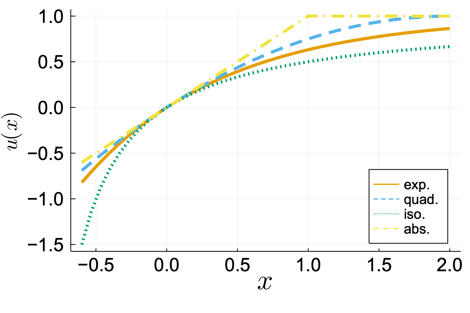
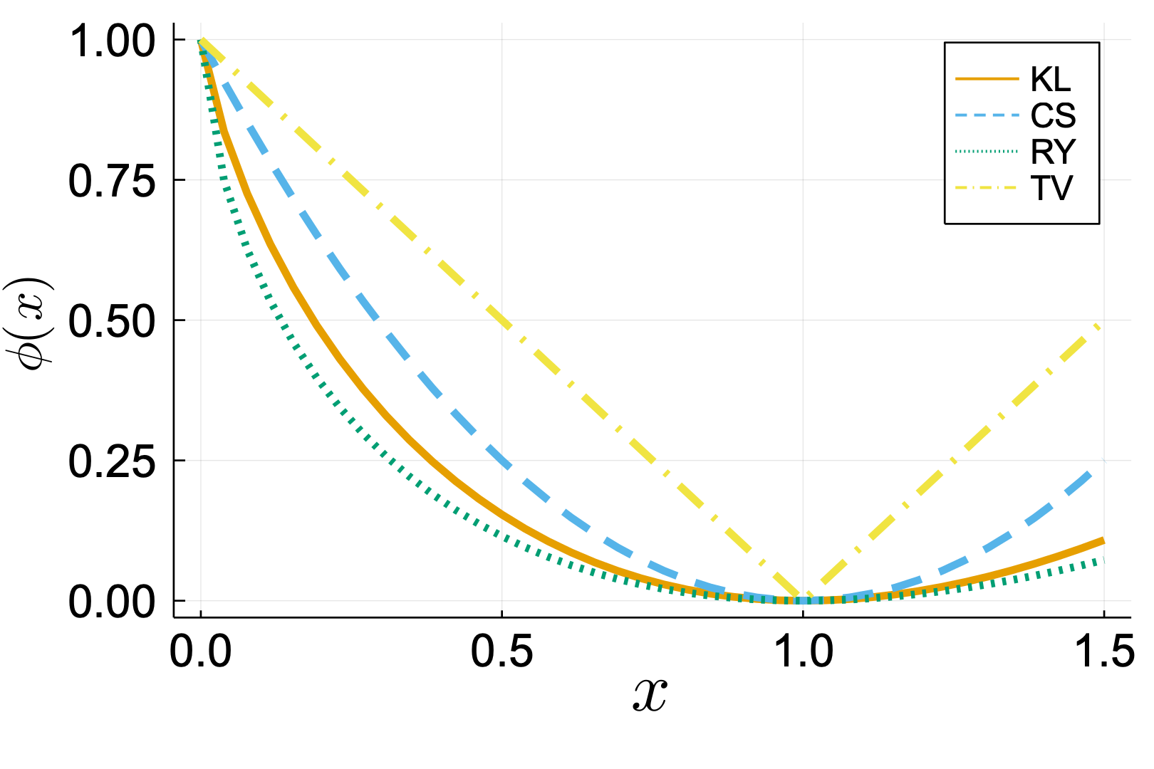
Figure 1: Four common disutility functions and their associated $\phi$-divergences: a) the exponential disutility (exp.) and Kullback-Leibler divergence (KL), b) a truncated quadratic disutility (quad.) and $\chi^{2}$ divergence (CS), c) the isoelastic disutility and Rényi divergence (RY), d) an absolute disutility and TV divergence (TV).

For the purpose of our theoretical results, and to facilitate the relationship between GVI and risk measures, we work in a slightly more general setting than traditional utility theory. We say that the functional $\mathcal{V}:\mathcal{M}\to[-\infty,+\infty]$ is a risk-averse expected disutility function if it satisfies:

• Convexity: $\mathcal{V}$ is proper, $\sigma(\mathcal{M},\mathcal{L})$-lower semicontinuous and convex;

• Risk Aversion: For any $X\in\mathcal{M}$, $\mathcal{V}(X)\geq\mathbb{E}[X]$ and $\mathcal{V}(X)=\mathbb{E}[X]$ implies $X\equiv 0$;

• Monotonicity: If $X,\,X^{\prime}\in\mathcal{M}$ satisfy $X\leq X^{\prime}$ a.s., then $\mathcal{V}(X)\geq\mathcal{V}(X^{\prime})$.

Commonly, $\mathcal{V}$ has the form

$$\mathcal{V}(X)=\mathbb{E}[v(X)],$$

where $v:\to[-\infty,+\infty]$ is a risk-averse disutility function. According to von Neumann and Morgenstern (2007), any “rational” decision maker has an expected disutility function that characterizes their decision when faced with risky outcomes. In their theory, the decision maker’s preference (denoted by the binary relationships $\prec$, $\succ$ and $\sim$) follows four axioms when deciding between any three random outcomes $X$, $Y$, and $Z$:

• Completeness: Either $X\prec Y$, $X\succ Y$ or $X\sim Y$;

• Transitivity: If $X\prec Y$ ($X\sim Y$) and $Y\prec Z$ ($Y\sim Z$), then $X\preceq Z$ ($X\sim Z$);

• Continuity: If $X\prec Y\prec Z$, then there exists $t\in[0,1]$ such that $tX+(1-t)Z\sim M$;

• Independence: If $X\prec Y$, then $tX+(1-t)Z\preceq tY+(1-t)Z$ for all $t\in(0,1]$.

Although the von Neumann-Morgenstern theory ensures the existence of an expected disutility function, it does not provide a constructive means to determine the disutility function. However, there have been attempts to systematically select a decision maker’s disutility function (Warren, 2019).

Analogously, we can generalize the $\phi$-divergence using the expected disutility functional $\mathcal{V}$ as $\Phi(p)=\mathcal{V}^{*}(p)$. Our next result lists the properties of $\Phi$ and demonstrates that $\Phi$ in fact defines a statistical divergence.

Proposition 1

Let the regret functional $\mathcal{V}:\mathcal{M}\to[-\infty,+\infty]$ satisfy (V1)–(V3). Then, the functional $\Phi:\mathcal{L}\to[-\infty,+\infty]$ defined by

$$\Phi(p)\triangleq\mathcal{V}^{*}(p)$$

is proper, $\sigma(\mathcal{L},\mathcal{M})$-lower semicontinuous, convex and satisfies the following properties:

1. $\Phi(p)\geq 0$ for all $p\in\mathcal{L}$;

2. $\Phi(p)=0$ if $p\equiv 1$ a.s.;

3. $\Phi(p)<\infty$ implies $p\geq 0$ a.s.;

4. If $\partial\mathcal{V}(0)=\{1\}$, then $\Phi(p)=0$ implies $p\equiv 1$ a.s.;

5. If $\partial\mathcal{V}(0)=\{1\}$, then $\mathrm{dom}\,\Phi=\{1\}$ if and only if $\mathcal{V}$ is positively homogeneous.

Proof  $\Phi$ is proper, $\sigma(\mathcal{L},\mathcal{M})$-lower semicontinuous and convex by the definition of the Fenchel conjugate (Rockafellar, 1971, pg. 188). Property 1 follows from the Fenchel-Young inequality and the fact that $\mathcal{V}(0)=0$, i.e.,

$$\Phi(p)=\Phi(p)+\mathcal{V}(0)=\Phi(p)+\Phi^{*}(0)\geq\mathbb{E}[0p]=0\quad\forall\,p\in\mathcal{L}.$$ (10)

Property 2 follows from (U2). That is, $X\mapsto\mathbb{E}[X]-\mathcal{V}(X)$ has a unique maximizer at $X\equiv 0$ with maximum value 0, and hence $\Phi(1)=\mathcal{V}^{*}(1)=0$. Property 3 follows from (U2) and (U3). First notice that

$$\mathcal{V}(X)\leq\mathcal{V}(0)=0\quad\forall\,X\leq 0\;\;\text{a.s.}$$

and let $p\in\mathcal{L}$ be such that $\Theta_{p}=\{\theta\in\Theta\,|\,p(\theta)<0\}$ has positive probability with respect to the prior, i.e., $\Pi(\Theta_{p})>0$. By setting

$$X_{p}(\theta)=\left\{\begin{array}[]{ll}-1&\text{if $\theta\in\Theta_{p}$}\\ 0&\text{otherwise}\end{array}\right.,$$

we see that $X_{p}\in\mathcal{M}$ since $\mathcal{M}$ includes all simple functions and

$$\mathbb{E}[tX_{p}p]-\mathcal{V}(tX_{p})\geq t\mathbb{E}[X_{p}p]>0\quad\forall\,t>0.$$

Taking the supremum in $t>0$ demonstrates that $\Phi(p)=+\infty$, proving property 3. For property 4, the Fenchel-Young inequality (10) holds with equality if and only if

$$0\in\partial\Phi(p)\quad\iff\quad p\in\partial\mathcal{V}(0).$$

and the desired result follows since $\partial\mathcal{V}(0)=\{1\}$ by assumption. Finally, to prove property 5, we first note that if $\mathrm{dom}\,\Phi=\{1\}$, then $\Phi$ is the indicator function of $\{1\}$ and hence $\mathcal{V}(X)=\Phi^{*}(X)=\mathbb{E}[X]$, which is positively homogeneous. On the other hand, if $\mathcal{V}$ is positively homogeneous, then $\Phi$ is an indicator function. Since $\Phi(p)>0$ unless $p\equiv 1$ a.s., we must have that $\Phi(p)=\infty$ unless $p\equiv 1$ a.s.  

Proposition 1 demonstrates that any risk-averse expected disutility function $\mathcal{V}$ that satisfies $\partial\mathcal{V}(0)=\{1\}$, defines the statistical divergence

$$D_{\Phi}(P\|\Pi)\triangleq\left\{\begin{array}[]{ll}\Phi(p)=\mathcal{V}^{*}(p)&\text{if $P\ll\Pi$ and $p\,\mathrm{d}\Pi=\mathrm{d}P$ with $p\in\mathcal{L}$}\\ +\infty&\text{otherwise}\end{array}\right..$$

$D_{\Phi}$ clearly generalizes the $\phi$-divergence since we can define $\Phi(p)=\mathbb{E}[\phi(p)]$ with $\phi(t)=v^{*}(t)$ and $\mathcal{V}(X)=\mathbb{E}[v(X)]$.

2.3 Risk Measures and Connections to Expected Disutility

A prinicpal contribution of this work is the demonstration of connections between GVI and risk measures. Risk measures are functionals used to quantify the overall loss or hazard associated with a random outcome. The concept of a risk measure is also closely linked to utility theory. In fact, given an expected disutility function $\mathcal{V}$, we can define the risk measure $\mathcal{R}:\mathcal{M}\to[-\infty,+\infty]$ projected from $\mathcal{V}$ by

$$\mathcal{R}(X)\triangleq\min_{t\in}\;\{t+\mathcal{V}(X-t)\}.$$ (11)

The class of risk measures projected from expected disutility functions as in (11) form a so-called risk quadrangle (Rockafellar and Uryasev, 2013) and are generalizations of optimized certainty equivalents (OCE) (Ben-Tal and Teboulle, 1986, 2007). In particualar, an OCE is a risk measure given by (11) with $\mathcal{V}(X)=\mathbb{E}[v(X)]$, where $v$ is a disutility function. It is common to require that a risk measure $\mathcal{R}$ satisfies some or all of the following axioms:

• Convexity: $\mathcal{R}$ is proper, $\sigma(\mathcal{M},\mathcal{L})$-lower semicontinuous and convex;

• Monotonicity: If $X,\,X^{\prime}\in\mathcal{M}$ satisfy $X\leq X^{\prime}$ a.s., then $\mathcal{R}(X)\geq\mathcal{R}(X^{\prime})$;

• Translation Equivariance: $\mathcal{R}(X+t)=\mathcal{R}(X)+t$ for all $X\in\mathcal{M}$ and $t\in$;

• Positive Homogeneity: $\mathcal{R}(tX)=t\mathcal{R}(X)$ for all $X\in\mathcal{M}$ and $t\geq 0$.

If $\mathcal{R}$ satisfies (R1)–(R3), it is referred to as a convex risk measure (Föllmer and Schied, 2002) and if it satisfies (R1)–(R4), it is coherent (Artzner et al., 1999). Coherent risk measures satisfy the worst-case expectation representation

$$\mathcal{R}(X)=\sup_{\eta\in\mathfrak{A}}\;\langle\eta,X\rangle_{\mathcal{M}^{*},\mathcal{M}},$$ (12)

where the risk envelope $\mathfrak{A}\subset\mathcal{M}^{*}$ is given by $\mathfrak{A}\triangleq\mathrm{dom}\,\mathcal{R}^{*}=\partial\mathcal{R}(0)$. Axiom (R1) ensures that $\mathfrak{A}$ is nonempty, closed and convex, while (R2) ensures that all $\eta\in\mathfrak{A}$ define nonnegative measures. In particular, let $B\in\mathcal{B}$ be such that $\langle\eta,\mathbbm{1}_{B}\rangle_{\mathcal{M}^{*},\mathcal{M}}<0$, where $\mathbbm{1}_{B}$ denotes the characteristic function of $B$, i.e., $\mathbbm{1}_{B}(\theta)=1$ if $\theta\in B$ and $\mathbbm{1}_{B}(\theta)=0$ if $\theta\not\in B$. Then, for any $X\in\mathrm{dom}\,\mathcal{R}$ and $t\in$, we have that

$$\mathcal{R}^{*}(\eta) \geq\sup_{t\in[0,+\infty)}\;\{\langle\eta,X-t\mathbbm{1}_{B}\rangle_{\mathcal{M}^{*},\mathcal{M}}-\mathcal{R}(X-t\mathbbm{1}_{B})\}$$

$$\geq\sup_{t\in[0,+\infty)}\;\{\langle\eta,X\rangle_{\mathcal{M}^{*},\mathcal{M}}-\mathcal{R}(X)-t\langle\eta,\mathbbm{1}_{B}\rangle_{\mathcal{M}^{*},\mathcal{M}}\}=+\infty.$$

Axiom (R3) ensures that $\eta\in\mathfrak{A}$ satisfies $\langle\eta,1\rangle_{\mathcal{M}^{*},\mathcal{M}}=1$. To see this, we have that for all $X\in\mathrm{dom}\,\mathcal{R}$ and $\eta\in\mathfrak{A}$,

$$\mathcal{R}^{*}(\eta) \geq\sup_{t\in}\,\{\langle\eta,X+t\rangle_{\mathcal{M}^{*},\mathcal{M}}-\mathcal{R}(X+t)\}$$

$$=\sup_{t\in}\,\{\langle\eta,X\rangle_{\mathcal{M}^{*},\mathcal{M}}-\mathcal{R}(X)+t(\langle\eta,1\rangle_{\mathcal{M}^{*},\mathcal{M}}-1)\}.$$

Consequently, $\mathcal{R}^{*}(\eta)=+\infty$ unless $\langle\eta,1\rangle_{\mathcal{M}^{*},\mathcal{M}}=1$. Hence, the risk envelope $\mathfrak{A}$ is a subset of probability measures in $\mathcal{M}^{*}$. Finally, owing to (R4), $\mathcal{R}^{*}$ is the indicator function of $\mathfrak{A}$. In general, we define the risk identifiers $p$ at $X\in\mathcal{M}$ as the subgradients of $\mathcal{R}$ at $X$, i.e., $p\in\partial\mathcal{R}(X)\subset\mathfrak{A}$. As a consequence of the Fenchel-Young inequality, the risk identifiers of a coherent risk measure $\mathcal{R}$ are the maximizers on the right-hand side of (12).

Returning to the generalized OCE (11), it is straightfoward to show that $\mathcal{R}$ is a convex risk measure if $\mathcal{V}$ is an risk-averse expected disutility function. Moreover, it is coherent if and only if $\mathcal{V}$ is positively homogeneous. To conclude this discussion, we prove fundamental relations between risk identifiers and subgradients of the regret function $\mathcal{V}$ as well as the Fenchel conjugates $\mathcal{R}^{*}$ and $\mathcal{V}^{*}$.

Lemma 2

Let $\mathcal{R}$ be defined by (11), where $\mathcal{V}$ is a risk-averse expected disutility function, and let $X\in\mathcal{M}$ be arbitrary. Denote by $\bar{t}\in$, a solution to the optimization problem defining $\mathcal{R}(X)$, i.e., $\mathcal{R}(X)=\bar{t}+\mathcal{V}(X-\bar{t})$. Then, we have that

$$\partial\mathcal{R}(X)=\partial\mathcal{V}(X-\bar{t})\cap\{p\in\mathcal{M}^{*}\,|\,\langle p,1\rangle_{\mathcal{M}^{*},\mathcal{M}}=1\}.$$

Proof  Let $p\in\partial\mathcal{R}(X)$, then $\langle p,1\rangle_{\mathcal{M}^{*},\mathcal{M}}=1$ by (R3) and for all $X^{\prime}\in\mathcal{M}$ and $t\in$, we have that

$$\{t+\mathcal{V}(X^{\prime}-t)\}-\{\bar{t}+\mathcal{V}(X-\bar{t})\}\geq\mathcal{R}(X^{\prime})-\mathcal{R}(X)\geq\langle p,(X^{\prime}-X)\rangle_{\mathcal{M}^{*},\mathcal{M}}.$$

Consequently, subtracting $(t-\bar{t})$ from both sides yields

$$\mathcal{V}(X^{\prime}-t)-\mathcal{V}(X-\bar{t})\geq\langle p,(X^{\prime}-t)-(X-\bar{t})\rangle_{\mathcal{M}^{*},\mathcal{M}}\quad\iff\quad p\in\partial\mathcal{V}(X-\bar{t}).$$

On the other hand, let $p\in\partial\mathcal{V}(X-\bar{t})$ satisfy $\langle p,1\rangle_{\mathcal{M}^{*},\mathcal{M}}=1$. By definition, we have that

$$\mathcal{V}(X^{\prime}-t)-\mathcal{V}(X-\bar{t})\geq\langle p,(X^{\prime}-t)-(X-\bar{t})\rangle_{\mathcal{M}^{*},\mathcal{M}}=\langle p,(X^{\prime}-X)\rangle_{\mathcal{M}^{*},\mathcal{M}}+(\bar{t}-t)$$

for all $X^{\prime}\in\mathcal{M}$ and all $t\in$. Subtracting $(\bar{t}-t)$ from both sides yields

$$t+\mathcal{V}(X^{\prime}-t)-\mathcal{R}(X)\geq\langle p,(X^{\prime}-X)\rangle_{\mathcal{M}^{*},\mathcal{M}}$$

and passing to the infimum over $t\in$ on the left-hand side proves the desired result.  

Lemma 3

Let $\mathcal{R}$ be defined by (11), where $\mathcal{V}$ is a risk-averse expected disutility function. Then, $\mathcal{R}^{*}$ is given by

$$\mathcal{R}^{*}(\eta)=\left\{\begin{array}[]{ll}\mathcal{V}^{*}(\eta)=\Phi(\eta)&\text{if $\langle\eta,1\rangle_{\mathcal{M}^{*},\mathcal{M}}=1$}\\ +\infty&\text{otherwise}\end{array}\right..$$

Proof  Using (11), we arrive at the following equality

$$\mathcal{R}^{*}(\eta) =\sup_{X\in\mathcal{M},\,t\in}\;\{\langle\eta,X\rangle_{\mathcal{M}^{*},\mathcal{M}}-\mathcal{R}(X-t)\}$$

$$=\sup_{Y\in\mathcal{M},\,t\in}\;\{\langle\eta,Y\rangle_{\mathcal{M}^{*},\mathcal{M}}-\mathcal{V}(Y)+t(\langle\eta,1\rangle_{\mathcal{M}^{*},\mathcal{M}}-1)\}$$

$$=\mathcal{V}^{*}(\eta)+\sup_{t\in}\;t(\langle\eta,1\rangle_{\mathcal{M}^{*},\mathcal{M}}-1).$$

The desired result then follows since the supremum in the final equality is equal to $+\infty$ unless $\langle\eta,1\rangle_{\mathcal{M}^{*},\mathcal{M}}=1$.  

3 Generalized Variational Inference as Risk Identification

In this section, we analyze the GVI problem

$$\sup_{p\in\mathfrak{D}}\;\{\mathbb{E}[pM_{N}]-\sigma\Phi(p)\},$$ (13)

where $\Phi$ is a generalized $\phi$-divergence as described in Proposition 1. In particular, our analysis provides necessary and sufficient conditions for the existence of solutions to (13), which we refer to as variational densities, and transforms the task of solving the optimization problem (13) into computing subgradients of a risk measure—a task that is generally simpler than optimization over probability density functions. We then introduce a new GVI problem, which we call coherent GVI (CGVI). CGVI is closely linked to coherent risk measures and again can be transformed into the problem of computing a risk identifer.

3.1 Existence and Asymptotics of Variational Densities

In this subsection, we provide necesary and sufficient conditions for the existence of solutions to the GVI problem (13). In doing so, we relate the optimization problem (13) to evaluating a generalized OCE and as a result of the Fenchel-Young inequality, show that the variational densities in (13) are subgradients of that OCE. The following result provides this characterization.

Theorem 4 (Existence of Variational Densities)

Let the generalized $\phi$-divergence $\Phi$ be defined using the risk-averse expected disutility function $\mathcal{V}$ as in Proposition 1, and let $\mathcal{R}$ denote the risk measure projected from $\mathcal{V}$ as in (11). Then, the GVI problem (13) has a solution if and only if

$$\partial\mathcal{R}(\sigma^{-1}M_{N})\cap\mathcal{L}\neq\emptyset$$

and the variational density is a risk identifier of $\sigma^{-1}M_{N}$, i.e.,

$$\bar{p}\in\partial\mathcal{R}(\sigma^{-1}M_{N})\cap\mathcal{L}.$$

Proof  We first notice that (13) is the Fenchel conjugate of $\sigma\Phi+\delta_{\mathfrak{D}}$. Consequently, the optimal value in (13) is the infimal convolution of the Fenchel conjugates $(\sigma\Phi)^{*}$ and $\delta_{\mathfrak{D}}^{*}$. That is, the optimal value in (13) is given by

$$\inf_{Y\in\mathcal{M}}\;\{(\sigma\Phi)^{*}(M_{N}-Y)+\delta_{\mathfrak{D}}^{*}(Y)\}.$$ (14)

Using the definition of $\Phi$, we have that $(\sigma\Phi)^{*}(Y)=\sigma\mathcal{V}(\sigma^{-1}Y)\triangleq\mathcal{V}_{\sigma}(Y)$. Moreover, the Fenchel conjugate of $\delta_{\mathfrak{D}}$ is the support function of $\mathfrak{D}$, i.e.,

$$\delta_{\mathfrak{D}}^{*}(Y)=\sigma_{\mathfrak{D}}(Y)=\sup_{p\in\mathfrak{D}}\mathbb{E}[pY]=\operatorname*{ess\,sup}Y,$$

where the last equality follows since $\mathfrak{D}$ consists of all probability density functions. Additionally, since $\mathcal{V}$ is monotonic and $Y\leq\operatorname*{ess\,sup}Y$ for all $Y\in\mathcal{M}$, we have that

$$\mathcal{V}_{\sigma}(M_{N}-Y)\geq\mathcal{V}_{\sigma}(M_{N}-\operatorname*{ess\,sup}Y)\quad\forall\,Y\in\mathcal{M}$$

and therefore, the random variable $Y$ in (14) can be replaced by a degenerate random variable (i.e., a scalar). The optimal value in (14) (and hence (13)) can thus be equivalently written as

$$\mathcal{R}_{\sigma}(M_{N})\triangleq\min_{t\in}\;\{t+\mathcal{V}_{\sigma}(M_{N}-t)\}=\sigma\mathcal{R}(\sigma^{-1}(M_{N}-t)),$$ (15)

where $\mathcal{R}$ is the risk measure defined in (11). As a result of the Fenchel-Young inequality, we have that

$$\mathcal{R}_{\sigma}(M_{N})=\langle p,M_{N}\rangle_{\mathcal{M}^{*},\mathcal{M}}-\mathcal{R}_{\sigma}^{*}(p)\quad\forall\,p\in\partial\mathcal{R}_{\sigma}(M_{N}).$$

Since $\mathcal{R}_{\sigma}(\cdot)=\sigma\mathcal{R}(\sigma^{-1}\cdot)$, we have that $\partial\mathcal{R}_{\sigma}(M_{N})=\partial\mathcal{R}(\sigma^{-1}M_{N})$ as desired.  

Remark 5 (Nonexistence)

In general, the estimation problem (13) need not have a solution in $\mathcal{L}$ since $\partial\mathcal{R}(\sigma^{-1}M_{N})\subseteq\mathcal{M}^{*}$. However, Theorem 12 guarantees that solutions exist when $\mathcal{L}=\mathcal{M}^{*}$ and $\partial\mathcal{R}(\sigma^{-1}M_{N})\neq\emptyset$.

The following two corollaries to Theorem 4 provide sufficient conditions for existence of variational densities to (13) when $\mathcal{L}=\mathcal{M}^{*}$ as discussed in Remark 5.

Corollary 6

In the setting of Theorem 4, if $\mathcal{L}=\mathcal{M}^{*}$ and $\mathcal{R}$ is finite valued and continuous at $\sigma^{-1}M_{N}$, then (13) has a solution.

Proof  Under the stated assumptions, $\partial\mathcal{R}(\sigma^{-1}M_{N})=\partial\mathcal{R}(\sigma^{-1}M_{N})\cap\mathcal{L}\neq\emptyset$ (Ekeland and Temam, 1999, Prop. 5.2) and the result of Theorem 4 ensures the existence of solutions.  

Corollary 7

In the setting of Theorem 4, if $\mathcal{L}=\mathcal{M}^{*}$ and $\mathcal{V}$ is finite valued, then (13) has a solution.

Proof  Since $\mathcal{V}$ is finite valued, $\mathcal{R}$ is also finite valued since $\mathcal{R}(Y)\leq\mathcal{V}(Y)$ for all $Y\in\mathcal{M}$. Therefore, $\mathcal{R}$ is continuous on $\mathcal{M}$ (Ekeland and Temam, 1999, Cor. 2.5). The corollary then follows from Corollary 6.  

Theorem 4 transforms the optimization problem (13) into a subdifferentiation problem involving the risk measure $\mathcal{R}$ projected from the risk-averse expected disutility function $\mathcal{V}$. Giving the connection between $\mathcal{R}$ and $\mathcal{V}$, it is possible to rewrite the condition $p\in\partial\mathcal{R}(\sigma^{-1}M_{N})$ in terms of $\mathcal{V}$.

Proposition 8

Consider the setting of Theorem 4 and let $\bar{t}$ be a minimizer in the definition of $\mathcal{R}_{\sigma}(M_{N})$, i.e.,

$$\mathcal{R}_{\sigma}(M_{N})=\min_{t\in}\;\{t+\sigma\mathcal{V}(\sigma^{-1}(M_{N}-t))\}.$$ (16)

Then, any solution to (13) satisfies

$$\bar{p}\in\partial\mathcal{V}(\sigma^{-1}(M_{N}-\bar{t}))\cap\{p\in\mathcal{L}\,|\,\mathbb{E}[p]=1\}.$$

Proof  This result follows directly from Theorem 4 and Lemma 2 applied to $\mathcal{R}_{\sigma}$.  

The final result in this section concerns the large data limit (i.e., as $N\to+\infty$) and presents a type of law of large numbers result for the variational densities $p_{N}$ associated with the payoff function $M_{N}$.

Theorem 9 (Asymptotic Consistency)

Consider the setting of Theorem 4. Let $\{\sigma_{N}\}\subset(0,\infty]$ with $\sigma_{N}\geq\sigma_{0}>0$ for all $N$ and $\{M_{N}\}$ satisfy $M_{N}\in\mathcal{M}$ a.s. Further, suppose that there exists $p_{N}\in\partial\mathcal{R}(\sigma_{N}^{-1}M_{N})\cap\mathcal{L}$ a.s. for all $N$ and that $\sigma_{N}^{-1}M_{N}\to M_{\star}$ in $\mathcal{M}$ a.s., i.e.,

$$\|\sigma_{N}^{-1}M_{N}-M_{\star}\|_{\mathcal{M}}\to 0\quad\text{a.s.}$$

Then, any $\sigma(\mathcal{L},\mathcal{M})$-accumulation point, $p_{\star}$, of the variational densities $\{p_{N}\}$ satisfies

$$p_{\star}\in\partial\mathcal{R}(M_{\star})\cap\mathcal{L}\quad\text{a.s.}$$

In particular, $p_{\star}$ is a variational density for the asymptotic GVI problem

$$\max_{p\in\mathfrak{D}}\;\{\mathbb{E}[pM_{\star}]-\Phi(p)\}.$$

Proof  Outside of a null set, this result follows from (Clarke, 1998, Prop. 2.1.5(b)).  

Remark 10 (Uniform Law of Large Numbers)

In Theorem 9, $M_{\star}$ is typically given by $\mathbb{E}_{y\sim Y}[m(\cdot,y)]$, where $\mathbb{E}_{y\sim Y}$ denotes the expectation with respect to the probability law of the noisy data $Y$ and $M_{N}=m(\cdot,y_{N})$ are generated by identically distributed realizations $y_{N}$ of $Y$. In this setting, the requirement that $\sigma_{N}^{-1}M_{N}\to M_{\star}$ in $\mathcal{M}$ a.s. is related to the uniform law of large numbers (LLN). In particular, if the uniform LLN holds and $\sigma_{N}\to\sigma_{\star}$, then $\sigma_{N}^{-1}M_{N}\to M_{\star}$ also holds. This is the case if, e.g., $\mathcal{M}$ is separable, $M_{N}$ and $m(\cdot,Y)$ are independent and identically distributed $\mathcal{M}$-valued random variables, and $\mathbb{E}_{y\sim Y}[\|m(\cdot,y)\|_{\psi^{\#}}]<\infty$ (Giné and Nickl, 2016, Cor. 3.7.21). This is also the case if, e.g., $\Theta$ is a compact subset of a Euclidean space, $\Upsilon$ is a Euclidean space, $m$ is a Carathèodory function and $m(\theta,\cdot)$ is dominated by an integrable function that is independent of $\theta$ (Jennrich, 1969, Th. 2).

3.2 Coherent Generalized Variational Inference

The risk measure $\mathcal{R}$ projected from $\mathcal{V}$ as in (11) satisifies (R1)–(R3). However, it need not be coherent unless $\mathcal{V}$ is positively homogeneous, in which case $\mathcal{V}_{\sigma}=\mathcal{V}$ and $\mathcal{R}_{\sigma}=\mathcal{R}$. That is, the learning rate $\sigma^{-1}$ has no effect on the estimation. This is a desirable property since choosing $\sigma$ can be difficult. In contrast to requiring $\mathcal{V}$ to be positively homogeneous, we can modify $\mathcal{R}_{\sigma}$ in the following way. Given $\varepsilon\geq 0$, we define the risk measure

$$\mathcal{R}^{\varepsilon}(X)\triangleq\inf_{\lambda>0}\;\{\lambda\varepsilon+\mathcal{R}_{\lambda}(X)\}$$ (17)

The risk measure $\mathcal{R}^{\varepsilon}$ inherits all properties from $\mathcal{R}$ with the addition that it is positively homogeneous, and hence coherent. Since $\mathcal{R}^{\varepsilon}$ is coherent, it satisfies

$$\mathcal{R}^{\varepsilon}(X)=\sup_{p\in\mathfrak{A}}\;\mathbb{E}[pX],$$ (18)

where the risk envelope $\mathfrak{A}$ is given by

$$\mathfrak{A}=\mathfrak{D}_{\varepsilon}\triangleq\{p\in\mathfrak{D}\,|\,\Phi(p)\leq\varepsilon\},$$ (19)

where $\Phi=\mathcal{V}^{*}$ is the generalized $\phi$-divergence associated with the regret functional $\mathcal{V}$. We refer to the optimization problem on the right-hand side of (18) with $X=M_{N}$ as the coherent GVI (CGVI) problem. Intuitively, the CGVI problem seeks a density function $p$ that maximizes the expected payoff $M_{N}$ within $\varepsilon$ of the prior distribution, when measured by the generalized $\phi$-divergence $\Phi$. For example, if $\mathcal{V}$ is the exponential disutility function, then $\mathcal{R}(X)=\log\mathbb{E}[\exp(X)]$ is the entropic risk measure and $\mathcal{R}^{\varepsilon}$ is the entropic value-at-risk. Moreover, $\Phi=\mathcal{V}^{*}$ generates the KL divergence. Consequently, (18) seeks a probability density function that maximizes the expected payoff and is within $\varepsilon$ of $\Pi$ when measured by the KL divergence. An obvious extension is to replace $\mathcal{R}^{\varepsilon}$ with some arbitrary coherent risk measure, not necessarily of the form (17). This extension leads to the interpretation of CGVI as finding a density that maximizes the expected payoff from the set of admissible densities $\mathfrak{A}$. However, we will restrict our attention to (17) given it’s close ties with GVI.

The CGVI problem presents a trade-off between selecting the learning rate $\sigma^{-1}$ as in GVI and selecting the $\phi$-diveregence tolerance $\varepsilon$. Both tasks can be challenging, however, choosing $\varepsilon$ may be more intuitive in certain applications. For example, if one can sample from the Bayesian posterior $p_{\rm post}$, then we can choose $\varepsilon>\Phi(p_{\rm post})$, ensuring that the CGVI density $\bar{p}$ improves upon the traditional Bayesian solution. In addition, if an intuitive method for choosing $\varepsilon$ exists, then the CGVI formulation determines an optimal inverse learning rate by solving for $\lambda$ in the definition of $\mathcal{R}^{\varepsilon}$.

Our first result proves that the risk envelope is indeed given by (19).

Proposition 11

The risk envelope of $\mathcal{R}^{\varepsilon}$ for $\varepsilon\geq 0$ is given by (19).

Proof  First, notice that for any $p\in\mathcal{M}^{*}$, we have

$$(\mathcal{R}^{\varepsilon})^{*}(p)=\sup_{X\in\mathcal{M},\,\lambda>0}\{\mathbb{E}[pX]-\lambda\varepsilon-\mathcal{R}_{\lambda}(X)\}=\sup_{\lambda>0}\lambda(\mathcal{R}^{*}(p)-\varepsilon).$$

Consequently, $(\mathcal{R}^{\varepsilon})^{*}(p)$ is finite if and only if $\Phi(p)\leq\varepsilon$ and $\langle p,1\rangle_{\mathcal{M}^{*},\mathcal{M}}=1$. Finally, $p\in\mathfrak{A}$ satisfies $p\geq 0$ a.s. since $\mathcal{R}^{\varepsilon}$ is monotonic as demonstrated in Section 2.3.  

Proposition 11 provides the intuitive interpretation of CGVI: maximize the expected payoff while being with $\varepsilon$ of the prior. Analogous to Theorem 4, the following result provides a necessary and sufficient condition for the existence of variational densities.

Theorem 12 (Existence of Variational Densities)

Let the generalized $\phi$-divergence $\Phi$ be defined using the risk-averse expected disutility function $\mathcal{V}$ as in Proposition 1 and let $\mathcal{R}^{\varepsilon}$ be defined as in (17) using the risk measure $\mathcal{R}$ projected from $\mathcal{V}$ as in (11). Then, the CGVI problem is given by

$$\mathcal{R}^{\varepsilon}(M_{N})=\sup_{p\in\mathfrak{D}_{\varepsilon}}\;\mathbb{E}[pM_{N}]=\min_{\mu\in,\,\lambda\geq 0}\;\{\mu+\lambda\varepsilon+(\lambda\Phi)^{*}(M_{N}-\mu)\},$$ (20)

and a variational density exists if and only if

$$\partial\mathcal{R}^{\varepsilon}(M_{N})\cap\mathcal{L}\neq\emptyset.$$

Moreover, the variational densities are given by

$$\bar{p}\in\partial\mathcal{V}(\bar{\lambda}^{-1}(M_{N}-\bar{\mu}))\cap\{p\in\mathcal{L}\,|\,\mathbb{E}[p]=1\},$$

where $(\bar{\mu},\bar{\lambda})$ solve the minimization problem on the right-hand side of (20).

Proof  The proof of this fact follows from the Fenchel-Young inequality, similar to the proof of Theorem 4.  

As in Remark 5, solutions to (20) may not exist if $\mathcal{M}=\mathcal{L}^{*}$, even if $\partial^{\varepsilon}\mathcal{R}(M_{N})\neq\emptyset$. The following two corollaries to Theorem 12 provide sufficient conditions for existence of variational densities to (20) when $\mathcal{L}=\mathcal{M}^{*}$.

Corollary 13

In the setting of Theorem 12, if $\mathcal{L}=\mathcal{M}^{*}$ and $\mathcal{R}^{\varepsilon}$ is finite valued and continuous at $M_{N}$, then (20) has a solution.

Proof  The proof of this fact is analogous to the proof of Corollary 6.  

Corollary 14

In the setting of Theorem 12, if $\mathcal{L}=\mathcal{M}^{*}$ and $\mathcal{V}$ is finite valued, then (13) has a solution.

Proof  The proof of this fact is analogous to the proof of Corollary 7.  

The final result in this section concerns the large data limit (i.e., as $N\to+\infty$) and presents type of law of large numbers for the CGVI densities $p_{N}$ associated with the payoff function $M_{N}$.

Theorem 15 (Asymptotic Consistency)

Consider the setting of Theorem 12 and suppose that $\mathcal{R}$ is finite valued on $\mathcal{M}$. Let $\{\varepsilon_{N}\}\subset[0,+\infty)$ and $\{M_{N}\}$ satisfy $M_{N}\in\mathcal{M}$ a.s. Furthermore, suppose that there exists $p_{N}\in\partial\mathcal{R}^{\varepsilon_{N}}(M_{N})\cap\mathcal{L}$ a.s. for all $N$, that $\varepsilon_{N}\to\varepsilon\geq 0$ and that $M_{N}\to M_{\star}$ in $\mathcal{M}$ a.s. Then, any $\sigma(\mathcal{L},\mathcal{M})$-accumulation point, $p_{\star}$, of the variational densities $\{p_{N}\}$ satisfies

$$p_{\star}\in\partial\mathcal{R}^{\varepsilon}(M_{\star})\cap\mathcal{L}.$$

In particular, $p_{\star}$ solves the asymptotic CGVI problem

$$\max_{p\in\mathfrak{D}_{\varepsilon}}\;\mathbb{E}[pM_{\star}].$$

Proof  To prove this result, we first demonstrate that $\mathcal{R}^{\varepsilon_{N}}$ converges to $\mathcal{R}^{\varepsilon}$ with respect to the slice topology. If so, then $\partial\mathcal{R}^{\varepsilon_{N}}$ graph converges $\partial\mathcal{R}^{\varepsilon}$ (Attouch and Beer, 1993, Th. 4.2). Suppose this is the case, then for all $X\in\mathcal{M}$ and $\eta\in\partial\mathcal{R}^{\varepsilon}(X)$ there exists $(X_{N},\eta_{N})$ with $\eta_{N}\in\partial\mathcal{R}^{\varepsilon_{N}}(X_{N})$ for all $N$ such that $\eta=\lim_{N}\eta_{N}$ in $\mathcal{M}^{*}$ and $X=\lim_{N}X_{N}$ in $\mathcal{M}$. Let $\{(M_{N},p_{N})\}$ denote a subsequence (without relabeling) on which $p_{\star}=\operatorname{\sigma(\mathcal{L},\mathcal{M})-lim}_{N}p_{N}$. Since $\mathcal{R}^{\varepsilon^{\prime}}$ is convex for all $\varepsilon^{\prime}\geq 0$, $\partial\mathcal{R}^{\varepsilon^{\prime}}$ is maximally monotone. Consequently, we have that

$$\langle p_{N}-\eta_{N},M_{N}-X_{N}\rangle_{\mathcal{M}^{*},\mathcal{M}}\geq 0\quad\text{a.s.}\quad\forall\,N.$$

Since $(M_{\star}-X)=\lim_{N}(M_{N}-X_{N})$ a.s. in $\mathcal{M}$ and $(p_{\star}-\eta)=\operatorname{\sigma(\mathcal{L},\mathcal{M})-lim}_{N}(p_{N}-\eta_{N})$, we have that

$$\langle p_{\star}-\eta,M_{\star}-X\rangle_{\mathcal{M}^{*},\mathcal{M}}\geq 0\quad\text{a.s.}$$

Since this holds for all $(X,\eta)$ with $\eta\in\partial\mathcal{R}^{\varepsilon}(X)$, we have that $p_{\star}\in\partial\mathcal{R}^{\varepsilon}(M_{\star})$ by the maximal monotonicity of $\partial\mathcal{R}^{\varepsilon}$, as desired.

To prove slice convergence, we must show that

1. $\forall\,X\in\mathcal{M}$, $\exists\,X_{N}\to X$ in $\mathcal{M}$ such that $\mathcal{R}^{\varepsilon_{N}}(X_{N})\to\mathcal{R}^{\varepsilon}(X)$;

2. $\forall\,p\in\mathcal{M}^{*}$, $\exists\,p_{N}\to p$ in $\mathcal{M}^{*}$ such that $(\mathcal{R}^{\varepsilon_{N}})^{*}(p_{N})\to(\mathcal{R}^{\varepsilon})^{*}(p)$

(Attouch and Beer, 1993, Th. 3.1). We will prove that $\varepsilon\mapsto\mathcal{R}^{\varepsilon}(X)$ is continuous for fixed $X\in\mathcal{M}$ by first proving that it is concave. Let $\varepsilon_{1},\,\varepsilon_{2}\geq 0$ and $t\in[0,1]$, then

$$\mathcal{R}^{t\varepsilon_{1}+(1-t)\varepsilon_{2}}(X)=\inf_{\lambda>0}\{t(\varepsilon_{1}\lambda+\mathcal{R}_{\lambda}(X))+(1-t)(\varepsilon_{2}\lambda+\mathcal{R}_{\lambda}(X))\}\geq t\mathcal{R}^{\varepsilon_{1}}(X)+(1-t)\mathcal{R}^{\varepsilon_{2}}(X).$$

Moreover, since $\mathcal{R}^{\varepsilon^{\prime}}(X)\leq\varepsilon^{\prime}+\mathcal{R}(X)<+\infty$ for all $\varepsilon^{\prime}\geq 0$, $\varepsilon\mapsto\mathcal{R}^{\varepsilon}(X)$ is finite valued, concave, and hence continuous on $[0,+\infty)$. Consequently, we can take $X_{N}=X$ for all $N$, which proves the first condition.

To prove the second, we note that for any $\varepsilon^{\prime}\geq 0$, $(\mathcal{R}^{\varepsilon^{\prime}})^{*}$ is the indicator function of $\mathfrak{D}_{\varepsilon^{\prime}}$. If $\varepsilon=0$, then $\mathfrak{D}_{0}=\{\pi\}$ and the result is trivial. We therefore assume $\varepsilon>0$. Let $p\in\mathcal{L}\setminus\mathfrak{D}_{\varepsilon}$, then $\delta_{\mathfrak{D}_{\varepsilon_{N}}}(p)=+\infty$ for $N$ sufficiently large since either $p\not\in\mathfrak{D}$ or $\Phi(p)>\varepsilon$. In this case, we can take $p_{N}=p$ for all $N$ to verify the second condition. On the other hand, suppose $p\in\mathfrak{D}_{\varepsilon}$ and define

$$p_{N}=\left\{\begin{array}[]{ll}p&\text{if $\varepsilon_{N}\geq\varepsilon$}\\ \tfrac{\varepsilon_{N}}{\varepsilon}p+(1-\tfrac{\varepsilon_{N}}{\varepsilon})&\text{if $\varepsilon_{N}>\varepsilon$}\end{array}\right..$$

Owing to convexity and the fact that $\Phi(1)=0$, we have $\Phi(p_{N})\leq\varepsilon_{N}$ for all $N$. Moreover, we clearly have that $p_{N}\to p$ and $\delta_{\mathfrak{D}_{\varepsilon_{N}}}(p_{N})=0$ for all $N$, proving the second condition.  

3.3 Application to $\phi$-Divergence-Based Variational Inference

In this subsection, we analyze GVI (13) and CGVI (20) problems when $\Phi$ is a $\phi$-divergence, i.e., $\Phi(p)=\mathbb{E}[\phi(p)]$. Recall that $\phi:\to[0,+\infty]$ is a proper, closed and convex function satisfying $\phi(1)=0$ and $\phi(t)=\infty$ for $t<0$. Moreover, $\phi$ generates a risk-averse regret function $v=\phi^{*}$. In this case, the GVI problem is

$$\mathcal{R}_{\sigma}(M_{N})=\sup_{p\in\mathfrak{D}}\;\left\{\mathbb{E}\left[pM_{N}\right]-\sigma\mathbb{E}[\phi(p)]\right\}$$ (21)

and the CGVI problem is

$$\mathcal{R}^{\varepsilon}(M_{N})=\sup_{p\in\mathfrak{D}}\;\left\{\,\mathbb{E}[pM_{N}]\,|\,\mathbb{E}[\phi(p)]\leq\varepsilon\,\right\}.$$ (22)

The natural function spaces in which to analyze (21) and (22) are the Orlicz spaces (Edgar and Sucheston, 1992). To introduce the Orlicz spaces that we will use, we first recall that the regret function $v$ associated with $\phi$ is proper, closed, convex, increasing, and satisfies $v(0)=0$. Consequently, $v$ is an Orlicz function as long as there exists $t>0$ such that $v(t)<+\infty$ (Rubshtein et al., 2016, Def. 13.1.1), which we assume to hold. We denote the Orlicz conjugate (also called the monotonic conjugate) of $v$ by $\psi=v^{\#}$, i.e.,

$$\psi(x)\triangleq\sup_{t\geq 0}\{tx-v(t)\}.$$

A straightforward calculation demonstrates that the Orlicz conjugate of $v$ is given by

$$\psi(x)=\left\{\begin{array}[]{ll}0&\text{if $x<1$}\\ \phi(x)&\text{if $x\geq 1$}\\ \end{array}\right..$$

and $\psi^{\#}=v$. We employ the Orlicz spaces generated by $\psi$ and $\psi^{\#}$ to analyze (21) and (22).

Recall that the Orlicz space $L_{\psi}\triangleq L_{\psi}(\Theta,\mathcal{B},\Pi)$ is the linear space of equivalence classes of $\mathcal{B}$-measurable functions $X$, equal up to a set of measure zero, such that $\mathbb{E}[\psi(|X/a|)]<\infty$ for some $a>0$ and that $L_{\psi}$ is a decomposable Banach lattice when endowed with the Luxemburg norm

$$\|X\|_{\psi}\triangleq\inf\{\,a>0\,|\,\mathbb{E}[\psi(|X/a|)]\leq 1\,\}.$$

We similarly define the Orlicz space $L_{\psi^{\#}}\triangleq L_{\psi^{\#}}(\Theta,\mathcal{B},\Pi)$. We pair $L_{\psi}$ with $L_{\psi^{\#}}$ using the bilinear form $\langle p,X\rangle\triangleq\mathbb{E}[pX]$ for $p\in L_{\psi}$ and $X\in L_{\psi^{\#}}$, which is finite by Young’s inequality. In this setting, $\mathfrak{D}_{\varepsilon}\subset L_{\psi}$ is bounded and $\sigma(L_{\psi},L_{\psi^{\#}})$-closed (see Appendix A). Here, $\mathcal{L}=L_{\psi}$ is the space of possible CGVI densities and $\mathcal{M}=L_{\psi^{\#}}$ is the space of pay-off functions $M_{N}$. Notice that $\mathcal{R}$ and $\mathcal{R}^{\varepsilon}$ are finite valued on $\mathcal{M}$ by definition and hence are continuous and subdifferentiable. However, this does not guarantee existence of solutions unless, e.g., $\mathcal{L}=\mathcal{M}^{*}$ is reflexive.

Our next results are corollaries of Theorems 4 and 12 that provide a semi-analytic expression for the variational densities of (21) and (22) and well as techincal assumptions on $v$ and $\psi$ that ensure existence of these densities.

Theorem 16 (Form of $\phi$-Divergence Densities)

Let $\mathcal{V}(\cdot)=\mathbb{E}[v(\cdot)]$, where $v=\phi^{*}$. If a variational density $\bar{p}\in\mathcal{L}$ exists for (21), then it satisfies

$$\bar{p}(\theta)\in\partial v(\sigma^{-1}(M_{N}(\theta)-\bar{t})),$$

where $\bar{t}$ solves the optimization problem in (16). On the other hand, if a variational density $\bar{p}\in\mathcal{L}$ exists for (22), then it satisfies

$$\bar{p}(\theta)\in\partial v(\bar{\lambda}^{-1}(M_{N}(\theta)-\bar{\mu})),$$ (23)

where $(\bar{\lambda},\bar{\mu})$ solves the optimization problem in (20).

Corollary 17 (Existence of $\phi$-Divergence Densities)

Consider the setting of Theorem 16 and suppose $v$ and $\psi$ are both finite valued and satisfy the ($\Delta_{2}$) condition, i.e., there exists $x_{0}>0$ and $k\in$ such that

$$v(2x)<kv(x)\qquad\text{and}\qquad\psi(2x)<k\psi(x)\qquad\forall\,x\geq x_{0}.$$

Then, variational densities exist to (21) and (22).

Proof  By construction we have that $\mathcal{R}$ and $\mathcal{R}^{\varepsilon}$ are continuous and subdifferentiable. Moreover, the stated assumptions on $v$ and $\psi$ ensure that $\mathcal{L}=\mathcal{M}^{*}$ is reflexive. Consequently, solutions exist by Corollaries 7 and 14.  

Corollary 17 demonstrates that the GVI problems (21) and (22) are well-posed, under certain assumptions on $v$ and $\psi$, for a fixed set of data $\{y_{n}\}_{n=1}^{N}$. Moreover, Theorem 16 provides an explicit representation of the variational densities. It is important to note that when $v=\phi^{*}$ is differentiable and $\bar{\lambda}>0$, these representations simplify to

$$\bar{p}(\theta)=v^{\prime}\left(\frac{M_{N}(\theta)-\bar{t}}{\sigma}\right)\qquad\text{and}\qquad\bar{p}(\theta)=v^{\prime}\left(\frac{M_{N}(\theta)-\bar{\mu}}{\bar{\lambda}}\right)$$

for (21) and (22), respectively.

3.4 Examples

To illustrate the connections between disutility functions, risk measures and CGVI, we present four common $\phi$-divergence examples. We note that the choice of $\phi$ should be left to the practitioner as it is application dependent and based on their disutility function. As such, we do not provide recommendations on how to choose $\phi$, but rather provide discussion for four common choices of $\phi$.

3.4.1 Kullback-Leibler Divergence

The KL divergence is generated by $\phi(t)=t\log(t)-t+1$ for $t\geq 0$, in which case $v(t)=e^{t}-1$ is the exponential disutility function (8) with $r=1$. See the solid orange line in Figure 1. For fixed $\sigma>0$, we can solve the one-dimensional minimization problem in (16) with $\mathcal{V}$ replaced by $\mathcal{V}_{\sigma}$, which yields $\bar{t}=\sigma\log\mathbb{E}[\exp(\sigma^{-1}M_{N})]$ (and similarly $\bar{\mu}=\bar{\lambda}\log\mathbb{E}[\exp(\bar{\lambda}^{-1}M_{N})]$). The associated risk measure $\mathcal{R}$ is the entropic risk measure and $\mathcal{R}^{\varepsilon}$ is the entropic value-at-risk (Ahmadi-Javid, 2012). Given $\sigma>0$ or the optimal $\bar{\lambda}>0$ from (20), we can compute the GVI and CGVI densities as

$$\bar{p}(\theta)=\frac{\exp\left(\sigma^{-1}M_{N}(\theta)\right)}{\mathbb{E}\left[\exp\left(\sigma^{-1}M_{N}\right)\right]}\qquad\text{and}\qquad\bar{p}(\theta)=\frac{\exp\left(\bar{\lambda}^{-1}M_{N}(\theta)\right)}{\mathbb{E}\left[\exp\left(\bar{\lambda}^{-1}M_{N}\right)\right]},$$

respectively. See Figure 2(a) for an example of the CGVI density. Note that the GVI and CGVI densities are exactly the Gibbs posterior with learning rate $\sigma^{-1}=\bar{\lambda}^{-1}$ for CGVI. Given the relation between KL-divergence-based GVI and the Gibbs posterior, it is natural to ask if there exists an $\varepsilon$ that produces the Bayesian posterior when $M_{N}$ is a log-likelihood function. The following result addresses this question.

Proposition 18 (Optimality of Bayesian Posterior)

Suppose the pay-off function $M_{N}$ is a log-likelihood function with $M_{N}\in L_{\psi^{\#}}$ and set

$$\varepsilon=D_{\rm KL}(\exp(M_{N})/\mathbb{E}[\exp(M_{N})]\|\pi).$$

Then, the CGVI variational density $\bar{p}$ with $\Phi$ given by the KL divergence is the usual Bayesian posterior. In particular, $\bar{\lambda}=1$.

Proof  This result follows by first differentiating the scalar function

$$\lambda\mapsto\lambda\varepsilon+\lambda\log\mathbb{E}[\exp(\lambda^{-1}M_{N})].$$

Since $\lambda=1$ is strictly interior in the set $[0,\infty)$, the desired optimality conditions consist of setting the aforementioned derivative to zero and setting $\lambda=1$. In doing so, we see that $\varepsilon$ must be as stated and we recover the Bayesian posterior as $\bar{p}$.  

3.4.2 $\chi^{2}$ Divergence

For the $\chi^{2}$-divergence, $\phi(t)=(t-1)^{2}$ for $t\geq 0$ and $\mathfrak{D}_{\varepsilon}$ can be equivalently rewritten as

$$\mathfrak{D}_{\varepsilon}=\{\,p\in\mathfrak{D}\,|\,\mathbb{E}[(p-1)^{2}]\leq\varepsilon\,\}=\{\,p\in\mathfrak{D}\,|\,\mathbb{E}[p^{2}]\leq 1+\varepsilon\,\}.$$

This follows from expanding the quadratic $\mathbb{E}[(p-1)^{2}]$ and noting that $\mathbb{E}[p]=1$. The set $\mathfrak{D}_{\varepsilon}$ defines the second-order higher moment coherent risk measure (see, e.g., § 8.2 in Cheridito and Li (2008)) with confidence level $\beta=1-(1+\varepsilon)^{-\frac{1}{2}}\in[0,1]$ and therefore

$$\mathcal{R}^{\varepsilon}(M_{N})=\min_{a\in}\left\{a+(1+\varepsilon)^{\frac{1}{2}}\mathbb{E}[\max\{0,M_{N}-a\}^{2}]^{\frac{1}{2}}\right\}.$$ (24)

Hence, given an optimal $\bar{a}$ from (24), we can recover the optimal density as

$$\bar{p}(\theta)=\frac{\max\left\{0,M_{N}(\theta)-\bar{a}\right\}}{\mathbb{E}\left[\max\left\{0,M_{N}-\bar{a}\right\}\right]}.$$

This follows from (Cheridito and Li, 2008, Prop. 3.2). See Figure 2(b) for an example of this density. An interesting property of the $\chi^{2}$-divergence (when compared with our other examples) is that the corresponding CGVI truncates the support of the posterior to account for $M_{N}(\theta)\geq\bar{a}$. Moreover, the associated disutility function for the $\chi^{2}$-divergence is the truncated quadratic disutility function

$$v(x)=\left\{\begin{array}[]{ll}\tfrac{1}{4}x^{2}+x&\text{if $x\geq-2$}\\ -1&\text{if $x<-2$}\end{array}\right.\qquad\implies\qquad v^{\prime}(x)=\max\{0,\tfrac{1}{2}x+1\}$$

and so the GVI density is given by

$$\bar{p}(\theta)=\frac{\max\{0,M_{N}(\theta)-(\bar{t}-2\sigma)\}}{\mathbb{E}[\max\{0,M_{N}-(\bar{t}-2\sigma)\}]}.$$

See the dashed blue line in Figure 1.

3.4.3 Rényi Divergence

The Rényi divergence (Rényi, 1961) is given by

$$D_{\alpha}(p\|\pi)\triangleq\frac{1}{\alpha-1}\log\mathbb{E}[p^{\alpha}],\quad\alpha>0,\;\alpha\neq 1$$

and $D_{\alpha}(p\|\pi)$ is the KL divergence when $\alpha=1$. The Rényi divergence is a popular alternative to the KL divergence because as demonstrated in (Knoblauch et al., 2019; Knoblauch, 2019), it often outperforms the KL divergence for GVI problems with misspecified priors. We restrict $\alpha$ to satisfy $0<\alpha<1$. After a sequence of invertible transformations, we can equivalently write the bound $D_{\alpha}(p\|\pi)\leq\varepsilon$ as

$$\frac{1}{\alpha-1}\mathbb{E}[p^{\alpha}-\alpha p+(\alpha-1)]\leq\frac{1-\exp((\alpha-1)\varepsilon)}{1-\alpha}=:\varepsilon_{\alpha},$$

producing a $\phi$-divergence on the left-hand side with $\phi(t)=(t^{\alpha}-\alpha t+(\alpha-1))/(\alpha-1)$ for $t\geq 0$ and $v(t)=(1+t/\beta)^{\beta}-1$ where $\beta=\frac{\alpha}{\alpha-1}<0$. This $\phi$-divergence is sometimes called the $\alpha$-divergence. The associated disutility function is the isoelastic disutility function (9). See the dotted green line in Figure 1. Given the optimal $\bar{t},\,\bar{\mu}\in$ and $\bar{\lambda}>0$, we can then compute the GVI and CGVI densities $\bar{p}$ as

$$\bar{p}(\theta)=\left(1+\frac{M_{N}(\theta)-\bar{t}}{\beta\sigma}\right)^{\beta-1}\qquad\text{and}\qquad\bar{p}(\theta)=\left(1+\frac{M_{N}(\theta)-\bar{\mu}}{\beta\bar{\lambda}}\right)^{\beta-1},$$

respectively. See Figure 2(c) for an example of the CGVI density.

3.4.4 Total-Variation Distance

For the total variation distance, we set $\phi(t)=|t-1|$ for $t\geq 0$. As shown in (Shapiro, 2017), the associated disutility function is

$$v(t)=\left\{\begin{array}[]{ll}\max\{0,t+1\}-1&\text{if $t\leq 1$}\\ +\infty&\text{if $t>1$}\end{array}\right.$$

See the dot-dashed yellow line in Figure 1. The Orlicz spaces generated by $\phi^{*}$ are $L_{\psi}=L^{1}(\Theta,\mathfrak{B},\Pi)$ and $L_{\psi^{\#}}=L^{\infty}(\Theta,\mathfrak{B},\Pi)$. As we will see, total-variation-based GVI and CGVI densities may not exist because the associated risk identifiers are measures that are not absolutely continuous with respect to $\Pi$ in general.

We first consider the total-variation-based CGVI problem. Upon the change of variables $s=\mu+\lambda\in$ and $t=\mu-\lambda\in$, we can equivalently rewrite (20) as

$$\min_{s,\,t\in} \left\{\tfrac{\varepsilon}{2}s+(1-\tfrac{\varepsilon}{2})t+\mathbb{E}[\max\{0,M_{N}-t\}]\right\}\quad\text{subject to}\quad\operatorname*{ess\,sup}M_{N}\leq s$$

$$=\tfrac{\varepsilon}{2}\operatorname*{ess\,sup}M_{N}+\min_{t\in}\left\{(1-\tfrac{\varepsilon}{2})t+\mathbb{E}[\max\{0,M_{N}-t\}]\right\},$$ (25)

where the optimal $s$ is $\bar{s}=\operatorname*{ess\,sup}M_{N}$ and the optimal $t$ solves the optimization problem in (25). Given $\bar{t}$, we recover $\bar{\mu}$ and $\bar{\lambda}$ as

$$\bar{\mu}=\tfrac{1}{2}(\operatorname*{ess\,sup}M_{N}+\bar{t})\qquad\text{and}\qquad\bar{\lambda}=\tfrac{1}{2}(\operatorname*{ess\,sup}M_{N}-\bar{t}).$$

Notice that if $\varepsilon\geq 2$, then (25) is simply $\operatorname*{ess\,sup}M_{N}$ and the optimal probability measures are convex combinations of point masses $\delta_{\theta^{\star}_{N}}$ centered at solutions $\theta^{\star}_{N}\in\Theta$ to (1) (here, $\delta_{\theta}$ denotes the usual Dirac measure, i.e., for any $S\in\mathcal{B}$, $\delta_{\theta}(S)=1$ if $\theta\in S$ and $\delta_{\theta}(S)=0$ if $\theta\not\in S$). On the other hand, if $0<\varepsilon<2$, then (25) can be equivalently rewritten as

$$\frac{\varepsilon}{2}\operatorname*{ess\,sup}M_{N}+\left(1-\frac{\varepsilon}{2}\right)\mathrm{AVaR}_{\varepsilon/2}\left(M_{N}\right),$$

where the average value-at-risk (AVaR) is defined by

$$\mathrm{AVaR}_{\beta}(X)\triangleq\frac{1}{1-\beta}\int_{\beta}^{1}q_{\alpha}(X)\,\mathrm{d}\alpha=q_{\beta}(X)+\frac{1}{1-\beta}\mathbb{E}[\max\{0,X-q_{\beta}(X)\}]$$

for $0<\beta<1$ and $q_{\alpha}(X)$ is the $\alpha$-quantile of the random variable $X$ (Rockafellar and Uryasev, 2002). In this case, the optimal $t$ is $\bar{t}=q_{\varepsilon/2}(M_{N})$. Moreover, the subdifferential $\partial\mathcal{R}^{\varepsilon}(M_{N})$ is generally set-valued and contains subgradients of the form, e.g.,

$$\frac{\varepsilon}{2}\delta_{\theta^{\star}_{N}}+\left(1-\frac{\varepsilon}{2}\right)P_{0},$$

where $P_{0}\in\mathfrak{P}$ is absolutely continuous with respect to $\Pi$ and has density $p_{0}\in\mathfrak{D}$ satisfying

$$p_{0}(\theta)\in\frac{1}{1-\frac{\varepsilon}{2}}\left\{\begin{array}[]{ll}\{0\}&\text{if $M_{N}(\theta)<\bar{t}$}\\ [0,1]&\text{if $M_{N}(\theta)=\bar{t}$}\\ \{1\}&\text{if $M_{N}(\theta)>\bar{t}$}\end{array}\right..$$

In particular, if $\Pi(\{\theta\in\Theta\,|\,M_{N}(\theta)=q_{\varepsilon/2}(M_{N})\})=0$, then

$$p_{0}(\theta)=\frac{1}{1-\frac{\varepsilon}{2}}\mathbbm{1}_{[0,\infty)}(M_{N}(\theta)-\bar{t}).$$

See Figure 2(d) for an example of this “density”. Unfortunately, the relationship between CGVI and AVaR is not present for the total-variation-based GVI problem (21). In this setting, we can make the substitution $s=t+\sigma$ in (16) to rewrite the GVI problem as

$$\min_{s\in}\;\{s+\mathbb{E}[\max\{0,M_{N}-s\}]\}\qquad\text{subject to}\qquad\operatorname*{ess\,sup}M_{N}-2\sigma\leq s.$$

Clearly, if $\tfrac{1}{2}(\operatorname*{ess\,sup}M_{N}-\operatorname*{ess\,inf}M_{N})\leq\sigma$, then we can set $\bar{s}=\operatorname*{ess\,inf}M_{N}$ and $\mathcal{R}_{\sigma}(M_{N})=\mathbb{E}[M_{N}]$. In this case, the variational density is $\bar{p}\equiv 1$. The more interesting case occurs when $\tfrac{1}{2}(\operatorname*{ess\,sup}M_{N}-\operatorname*{ess\,inf}M_{N})>\sigma$, which implies $\operatorname*{ess\,inf}M_{N}<\operatorname*{ess\,sup}M_{N}-2\sigma\leq\bar{s}\leq\operatorname*{ess\,sup}M_{N}$. Consequently, $\mathbb{E}[M_{N}]\leq\mathcal{R}_{\sigma}(M_{N})\leq\operatorname*{ess\,sup}M_{N}$. Moreover, we have that $\sigma\mapsto\mathcal{R}_{\sigma}(M_{N})$ is monotonically decreasing, attaining its lower bound when $\sigma=\tfrac{1}{2}(\operatorname*{ess\,sup}M_{N}-\operatorname*{ess\,inf}M_{N})$ and its upper bound when $\sigma=0$.

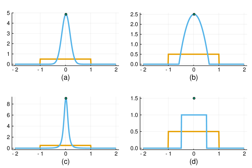
Figure 2: $\phi$-divergence CGVI densities for (a) KL, (b) $\chi^{2}$, (c) Rényi ($\alpha=\tfrac{1}{2}$), and (d) total variation. In this example, $\Upsilon=\Theta=$, 100 realizations of $Y$ were drawn from a standard normal distribution, $\Pi$ is the uniform measure on $[-1,1]$, $m$ is the standard normal log-likelihood function, and $\varepsilon=1$.

4 Computation, Sampling and Asymptotic Analysis

In this section, we investigate several theoretical properties that are relevant for the computation of the $\phi$-divergence-based CGVI variational densities analyzed in Subsection 3.3 and note that it may be possible to extend these results to general $\Phi$ using empirical estimates for law-invariant functionals (cf. (Shapiro et al., 2014, Ch. 7.2.6)). In practice, we can only expect to solve the one-dimensional GVI (21) and two-dimensional CGVI (22) problems approximately by either stochastic approximation algorithms or by empirical approximation using samples from the prior distribution $\Pi$. The latter is often referred to as sample average approximation (SAA) in stochastic programming. This raises important questions regarding the asymptotic behavior of the sample-based solutions as the sample size increases to infinity.

Given $S$ independent and identically distributed (iid) samples $\{\theta_{s}\}_{s=1}^{S}$ drawn from $\Pi$, we evaluate the pay-off samples $\{M_{N}^{s}\triangleq M_{N}(\theta_{s})\}_{s=1}^{S}$ and then solve the SAA problem

$$\widehat{\mathcal{R}}^{\varepsilon}_{S}(M_{N})\triangleq\inf_{\mu\in,\;\lambda\geq 0}\left\{\,\mu+\lambda\varepsilon+\frac{1}{S}\sum_{s=1}^{S}(\lambda\phi)^{*}(M_{N}^{s}-\mu)\right\}.$$ (26)

We denote the set of minimizers to (26) by $\widehat{X}^{\star}_{S}$ and the minimizers to (22) by $X^{\star}$. The optimization problem (26) is a two-dimensional convex optimization problem that can be solved using any convex programming methods. For example, one can employ proximal or projected (sub)gradient-type methods. If $\phi^{*}$ is sufficiently differentiable, one can employ Newton-type methods. See (Beck, 2017) for a survey of other applicable first-order methods. Additionally, under appropriate assumptions, one can prove that the estimators $\mu_{S}$ and $\lambda_{S}$ computed by solving (26) converge a.s. to a solution of (22), see e.g., (Dupacova and Wets, 1988; King and Rockafellar, 1993; Shapiro, 1989) and the result below. Moreover, when $\bar{\lambda}>0$, (Clarke, 1983, Prop. 2.1.5(b)) ensures that any $\sigma(L_{\psi},L_{\psi^{\#}})$-accumulation point $\bar{p}$ of the sequence $\{p_{S}\}$ with $p_{S}(\theta)\in\lambda_{S}\partial\phi^{*}((M_{N}(\theta)-\mu_{S})/\lambda_{S}),$ satisfies (23) a.s.

We emphasize here that there are no limitations on the dimensions of $\Theta$. In particular, the size of $\theta$ does not change the computational complexity of solving the two-dimensional convex optimization problem (26) since the pay-off samples $M_{N}(\theta_{s})$ are computed offline, prior to solving (26). However, it is important to note that the number of samples $S$ required to achieve a prescribed accuracy when solving the SAA problem (26) is typically dimension dependent (Shapiro et al., 2014, Chap. 5). Once $\bar{\lambda}$ and $\bar{\mu}$ are computed, we can generate samples from the CGVI distribution $\bar{p}$ using similar methods as those used in Bayesian inference such as Markov Chain Monte Carlo (MCMC) (Beskos et al., 2017) and transport maps (El Moselhy and Marzouk, 2012). We also note that for many choices of $\phi$, the density $\bar{p}$ is given in closed form once $\bar{\lambda}$ and $\bar{\mu}$ are computed. This allows us to compute various statistics such as the value of $\theta$ that maximizes $\bar{p}$.

In the next result, we prove asymptotic consistency of the optimal values and optimal solution set of (26) in the large sample limit (i.e., $S\to\infty$). These statements follow by verifying the assumptions of (Shapiro et al., 2014, Th. 5.4). We prove the various necessary conditions in Appendix B and then obtain the asymptotic consistency as a corollary. We refer the reader to (Rockafellar and Wets, 1998, Chap. 14) or (Shapiro et al., 2014, Chap. 7) regarding the terminology.

Theorem 19 (Asymptotic Consistency: Sample Limit)

If the asumptions of Corollary 16 hold, then

1. $\widehat{\mathcal{R}}^{\varepsilon}_{S}(M_{N})\to\mathcal{R}^{\varepsilon}(M_{N})$ a.s.;

2. The deviation of $\widehat{X}^{\star}_{S}$ to $X^{\star}$ converges to zero a.s. That is, we have that

   $$\mathbb{D}(\widehat{X}^{\star}_{S},X^{\star})\triangleq\sup_{(\mu,\lambda)\in\widehat{X}^{\star}_{S}}\inf_{(\mu^{\prime},\lambda^{\prime})\in X^{\star}}\|(\mu,\lambda)-(\mu^{\prime},\lambda^{\prime})\|\to 0\quad\text{a.s.}$$

Proof  This is a direct application of (Shapiro et al., 2014, Th. 5.4) in light of Theorem 23.  
Theorems 23 and 19 lead to the following observations. As proven in Theorem 23, the solution sets $X^{\star}$ and $\widehat{X}^{\star}_{S}$ are always nonempty, compact, and convex subsets of $\times[0,\infty)$, regardless of the sample size $S$. For any $(\mu_{S},\lambda_{S})\in\widehat{X}^{\star}_{S}$, there exists $(\mu_{S}^{\prime},\lambda_{S}^{\prime})\in X^{\star}$ satisfying

$$\|(\mu_{S},\lambda_{S})-(\mu^{\prime}_{S},\lambda^{\prime}_{S})\|=\min_{(\mu^{\prime},\lambda^{\prime})\in X^{\star}}\|(\mu_{S},\lambda_{S})-(\mu^{\prime},\lambda^{\prime})\|\leq\mathbb{D}(\widehat{X}^{\star}_{S},X^{\star})$$

since $X^{\star}$ is compact. Using again the compactness of $X^{\star}$, we can deduce the existence of some $(\bar{\mu},\bar{\lambda})\in X^{\star}$ and a subsequence $\{(\mu^{\prime}_{S_{k}},\lambda^{\prime}_{S_{k}})\}$ that converges to $(\bar{\mu},\bar{\lambda})$ a.s. It follows that

$$\|(\mu_{S_{k}},\lambda_{S_{k}})-(\bar{\mu},\bar{\lambda})\|\leq\mathbb{D}(\widehat{X}^{\star}_{S_{k}},X^{\star})+\|(\mu^{\prime}_{S_{k}},\lambda^{\prime}_{S_{k}})-(\bar{\mu},\bar{\lambda})\|$$

and, by Theorem 19, we have that

$$\|(\mu_{S_{k}},\lambda_{S_{k}})-(\bar{\mu},\bar{\lambda})\|\to 0\quad\text{a.s.}$$

Consequently, we have that

$$\mu_{S_{k}}+\varepsilon\lambda_{S_{k}}+\frac{1}{S_{k}}\sum_{k=1}^{S_{k}}(\lambda_{S_{k}}\phi)^{*}(M_{N}^{k}-\mu_{S_{k}})\to\bar{\mu}+\varepsilon\bar{\lambda}+\mathbb{E}[(\bar{\lambda}\phi)^{*}(M_{N}-\bar{\mu})]\quad\text{a.s.}.$$

In the following corollary, we use the above observations to relate the solutions $(\mu_{S},\lambda_{S})$ to sequences of CGVI variational densities.

Theorem 20

Let the assumptions of Corollary 16 hold and suppose $L_{\psi}$ is reflexive. If $\{\bar{p}_{k}\}$ denotes a sequence of SAA estimators to the CGVI posterior associated with $\{S_{k}\}$ samples with $S_{k}\nearrow\infty$, i.e.,

$$\bar{p}_{k}(\theta)\in\partial(\lambda_{S_{k}}\phi)^{*}(M_{N}(\theta)-\mu_{S_{k}}).$$

Then any a.s. $\sigma(L_{\psi},L_{\psi^{\#}})$-accumulation point $\bar{p}$ of $\{\bar{p}_{k}\}$ is a variational density for (22), i.e., $\bar{p}$ satisfies (23).

Proof  This proof uses various notions of variational convergence. See (Attouch, 1984) for an overview of these techniques. One can show that the sequence of functionals $\Phi_{k}(p)\triangleq\lambda_{S_{k}}\mathbb{E}[\phi(p)]$ pointwise and epi-converge to $\overline{\Phi}\triangleq\overline{\lambda}\mathbb{E}[\phi(\cdot)]$ a.s. (Shapiro et al., 2014, Sect. 7.2.5). Moreover, since $\langle\cdot,X\rangle:L_{\psi}\to$ is a continuous linear functional for any $X\in L_{\psi^{\#}}$, the sequence $\Phi_{k}(\cdot)-\langle\cdot,X\rangle$ also pointwise and epi-converge a.s. Consequently, we have that

$$\inf_{p\in L_{\psi}}\left\{\Phi_{k}(p)-\langle p,X\rangle\right\}\to\inf_{p\in L_{\psi}}\left\{\overline{\Phi}(p)-\langle p,X\rangle\right\}\quad\text{a.s.}$$

(Attouch, 1984). As a result, $(\Phi_{k})^{*}$ converges to $(\overline{\Phi})^{*}$ pointwise a.s. In fact, if $X_{k}\to X$ with respect to the $\sigma(L_{\psi^{\#}},L_{\psi})$-topology, then passing to the limit inferior (a.s.) on both sides and taking the supremum over $p$ in the inequality

$$-\inf_{p\in L_{\psi}}\left\{\Phi_{k}(p)-\langle p,X_{k}\rangle\right\}\geq-(\Phi_{k}(p)-\langle p,X_{k}\rangle)\quad\forall p\in L_{\psi}\quad\text{a.s.}$$

yields

$$\liminf_{k\to\infty}(\Phi_{k})^{*}(X_{k})\geq(\overline{\Phi})^{*}(X)\quad\text{a.s.},$$

since the pointwise and epi-limits of $\Phi_{k}$ coincide. These facts ensure that $(\Phi_{k})^{*}$ Mosco converges to $(\overline{\Phi})^{*}$ and therefore the subdifferentials $\partial(\Phi_{k})^{*}$ graph converge to $\partial(\overline{\Phi})^{*}$ by (Attouch, 1984, Th. 3.66). Lastly, we note that $M_{N}-\mu_{S_{k}}$ strongly converges in $L_{\psi^{\#}}$ a.s. Therefore, if $\overline{p}$ is an a.s. $\sigma(L_{\psi},L_{\psi^{\#}})$-accumulation point of $\left\{\bar{p}_{k}\right\}$ with $\overline{p}_{k}\in\partial(\Phi_{k})^{*}(M_{N}-\mu_{S_{k}})$, then $\overline{p}\in\partial(\overline{\Phi})^{*}(M_{N}-\bar{\mu})$ and by (Rockafellar, 1974, Th. 21), we have that

$$\bar{p}(\theta)\in\partial(\bar{\lambda}\phi)^{*}(M_{N}(\theta)-\bar{\mu})\quad\text{a.s.}$$

Due to Theorem 19, the discussion above surrounding the derivation of $(\mu_{S_{k}},\lambda_{S_{k}})$, and strong duality, $\bar{p}$ is optimal for (2).  

4.1 Performance of CGVI under Model Misspecification

As noted earlier, using other $\phi$-divergences such as the Rényi divergence in place of the KL divergence may produce better estimates of the parameters $\theta$. We demonstrate this feature with a small example in which both the prior and model are misspecified and only a small number of samples is available.

Given the data $\left\{y_{n}=(x_{n},z_{n})\right\}_{n=1}^{N}\subset\mathbb{R}^{2}$ with $N=100$, we postulate a linear decision function $h_{\theta}(x)=\theta x$ and make the assumption that the observation errors $\epsilon_{n}\triangleq z_{n}-h_{\theta^{\star}}(x_{n})$ are iid standard normal random variables. For the experiment, however, we generate the data using the heteroscedastic model

$$z_{n}=x_{n}+\sigma(x_{n})\eta_{n}$$

(i.e., $\theta^{\star}=1$), where $\eta_{n}$ are iid standard normal random variables and

$$\sigma(x)=\left\{\begin{array}[]{ll}0.04&\text{if $x<\xi^{N}_{5}$}\\ 0.4&\text{if $x\in[\xi^{N}_{5},\xi^{N}_{95}]$}\\ 1.0&\text{otherwise}\end{array}\right..$$

Here, $\xi^{N}_{5}$ and $\xi^{N}_{95}$ denote the 5% and 95% quantiles of the standard normal distribution, respectively. Using the standard normal error assumption, the log-likelihood function is

$$m(\theta,y_{n})=-\frac{1}{2}|z_{n}-\theta x_{n}|^{2}.$$

For the prior, we choose $\Pi$ to be normally distributed with mean -2 and unit variance. We note that the true parameter value $\theta^{\star}=1$ is in the support of $\Pi$, but it is more than two standard deviations from the mean.

For the $\phi$-divergence CGVI problems, we set $\varepsilon$ to be twice the $\phi$-divergence of the Bayesian posterior (BS) from the prior $\Pi$. We compute these values using $S=10,000$ samples of $\theta$ drawn from the prior for the KL, the $\chi^{2}$ (CS), and the Rényi (RY) with $\alpha=0.5$ divergences. We list the values of $\varepsilon$ in Table 1.

	BS	KL	CS	RY	TV
$\varepsilon$	—	1.991814	5.842229	1.106317	1.376138
$\eta$	1.632968	1.092635	1.579035	0.367454	0.108191

Table 1: The constraint tolerance $\varepsilon$ and parameter errors $\eta$ (to six significant digits) for the Bayesian postior (BS), the Kullback-Leibler divergence (KL), the $\chi^{2}$ divergence (CS), the Rényi divergence (RY), and the total variation distance (TV).

This choice of $\varepsilon$ ensures that the Bayesian posterior density is feasible for each of the CGVI problems. We then compute the optimal $\lambda_{S}$ and $\mu_{S}$ for each example. For KL and CS, we compute $\lambda_{S}$ and $\mu_{S}$, respectively, using Ridder’s root finding algorithm. For RY, we compute the optimal parameters using a projected gradient method. We plot these densities in the left image of Figure 3 along with their value at the true parameter $\theta^{\star}=1$. In each case, this value is slightly skewed to the right of the mode. In addition, we plot the full posterior densities in the right image of Figure 3.

For the total variation CGVI (TV), we proceed in a different manner. This is due to the fact that TV is fundamentally different than the other $\phi$-divergence examples as it includes point masses at the maximizers of $M_{N}$, i.e., the maximum likelihood estimators. For this one-dimensional example, these are easy to estimate. For larger dimensional problems, one would require a robust optimization method to solve the associated nonlinear program. To compute $\varepsilon$, we first compute the TV distance of the Bayesian posterior from the prior using a grid on $[-20,20]$ of size $S=100,000$. This value is listed in the rightmost column of Table 1. Scaling this value by two would yield a number larger than two. Consequently, the CGVI would only be comprised of convex combinations of point masses at the maximum likelihood estimators. Instead, we set $\varepsilon$ as in Table 1 and compute the $\varepsilon/2$ quantile, which we use to approximate the cumulative distribution function (cdf) of the full TV posterior, see Figure 4.

Finally, we judge the performance of the various CGVIs by estimating the mode of the posteriors and comparing them in absolute value to the true parameter value $\theta^{\star}=1$. We denote this error by $\eta$ and list the values in the second row of Table 1. As expected, the standard Bayesian posterior yields the worst estimate. This is followed by CS, despite exhibiting a smaller variances than the other CGVIs (see Figure 3). KL outperforms both of these. However, the clear winner amongst the CGVIs, other than TV, is RY, which corroborates the observations in (Knoblauch et al., 2019). Finally, we see that TV is the least susceptible to small data and misspecification as it provides the best estimate. However, it is more limited in applicability than RY as one must compute the maximum likelihood estimators and the quantiles of $M_{N}$.

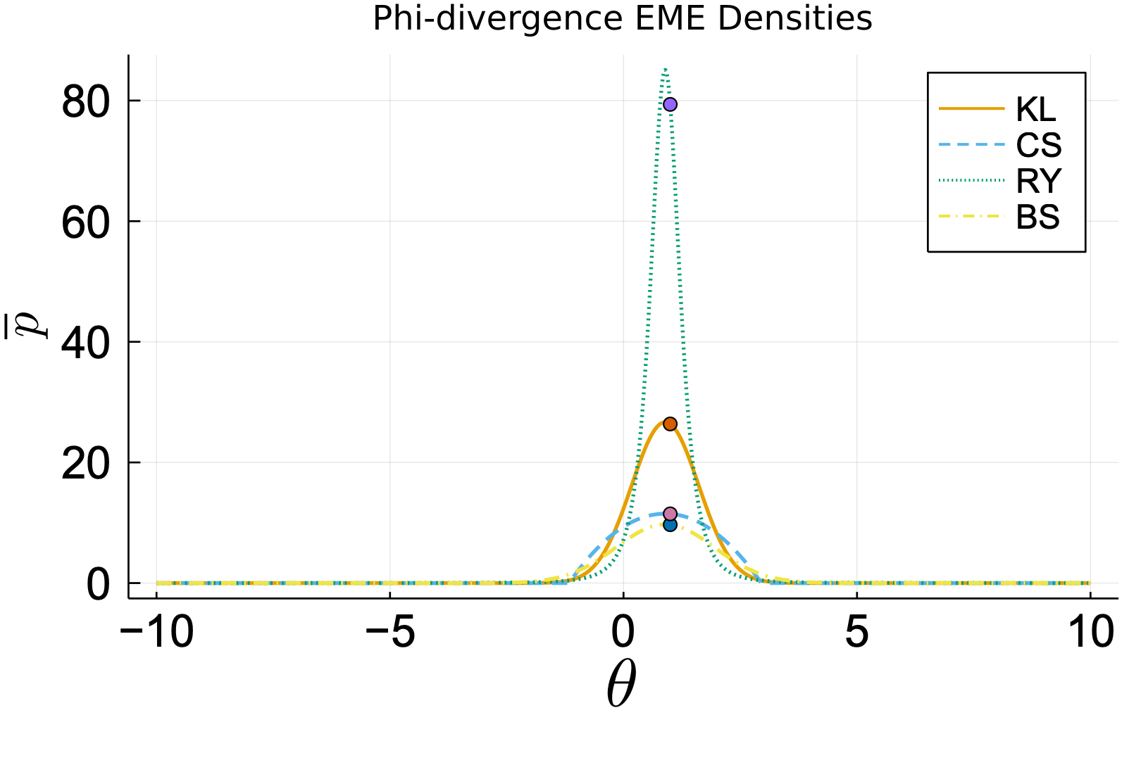
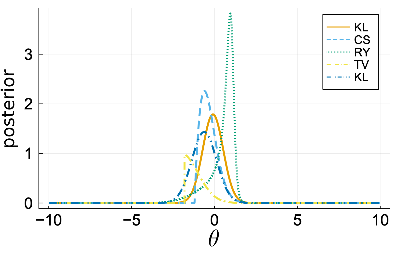
Figure 3: Left: CGVI densities for standard Bayes, KL, $\chi^{2}$ and Renyi ($\alpha=0.5$) divergences. Right: full posterior densities for standard Bayes, KL, $\chi^{2}$ and Renyi ($\alpha=0.5$)

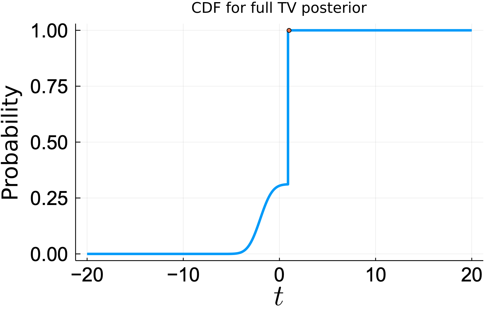
Figure 4: An empirical estimate of the cumulative distribution function for the TV posterior. The jump occurs at the estimated maximum likelihood estimator.

5 Empirical CGVI: An “Objective” Perspective

In this brief section, we present several extensions to CGVI in which we assume that no reasonable prior measure $\Pi$ exists. Instead, we wish to proceed in a more objective manner in which perhaps only samples of the prior or moments are available and we are unsure which utility function to choose. We introduce two approaches to handle this situation. The first approach falls into the class of problems described by (6) whereas the second approach is based on moment matching. From a computational standpoint, more regularity of $M_{N}$ and the integrands $\psi$ in the case of moment-matching would be necessary to compute the global minimizers. A deeper look into the computation of empirical CGVIs will be the subject of future investigations.

5.1 Wasserstein Distance and Empirical Priors

In this subsection, we assume that we have many noisy observations of $Y$ and a few noisy realizations of $\theta$. For example, these realizations could be the result of prior estimation attempts. This could also model the practical situation in which observations of $Y$ are cheap to obtain relative to observations of $\theta$. To formulate the estimation problem (2), we resort to empirical estimation to generate the prior distribution $\Pi$.

Let $\Theta$ be a locally $\sigma$-compact Polish space endowed with its Borel $\sigma$-algebra $\mathcal{B}$. According to (Williamson and Janos, 1987, Th. 1), $\Theta$ admits a metric $d:\Theta\times\Theta\to\mathbb{R}$ that has the Heine-Borel property (i.e., all closed and bounded sets are compact). One obvious example for such a $\Theta$ is ⁿ with the usual Euclidean topology. We further require that $M_{N}$ is bounded, continuous, and concave on $\Theta$. Given $M$ observations of $\theta$, denoted by $\{\widehat{\theta}_{m}\}_{m=1}^{M}$, we define the prior measure $\Pi$ as the empirical measure:

$$\Pi=\frac{1}{M}\sum_{m=1}^{M}\delta_{\widehat{\theta}_{m}},$$

One attractive approach to defining a meaningful set of measures $\mathfrak{A}$ in (2) is to use probability metrics, cf. (Rachev, 1991). To this end, we employ the Wasserstein-1 distance (i.e., the Kantorovich-Rubinstein metric), $W_{1}:\mathfrak{P}\times\mathfrak{P}\to[0,\infty]$, defined by

$$W_{1}(P,Q)\triangleq\inf_{\rho\in\Gamma(P,Q)}\int_{\Theta^{2}}d(\theta_{1},\theta_{2})\,\rho(\mathrm{d}\theta_{1},\mathrm{d}\theta_{2}),$$

where $\Gamma(P,Q)\subset\mathfrak{P}(\Theta\times\Theta)$ denotes the subset of all Borel probability measures on $\Theta\times\Theta$ that have marginal $P$ for their first factor and marginal $Q$ for their second. We then define the set $\mathfrak{A}$ by

$$\mathfrak{A}=\{\,P\in\mathfrak{P}\,|\,W_{1}(P,\Pi)\leq\varepsilon\,\}.$$

For this choice of $\mathfrak{A}$, we have the following existence result.

Theorem 21 (Existence of Wasserstein CGVI)

Under the stated assumptions, (2) admits a solution $P^{\star}$ for any $\varepsilon>0$.

Proof  Since $M_{N}$ is bounded and continuous, $\mathbb{E}_{P}\left[M_{N}\right]$ is continuous in $P\in\mathfrak{P}(\Theta)$ with respect to the weak-convergence of probability measures. It follows from (Pichler and Xu, 2018, Prop. 3) that $\mathfrak{A}$ is weakly compact. In order to use the proof of (Pichler and Xu, 2018, Prop. 3), we first note that $\mathcal{P}\triangleq\{\Pi\}$ is a uniformly tight set of probability measures. Moreover, according to (Williamson and Janos, 1987, Th. 1), given a compact set $C\subset\Theta$ and some constant $\delta>0$, the set $C_{\delta}\triangleq\left\{\theta\in\Theta\,|\,d(\theta,c)\leq\delta,c\in C\right\}$ is a closed and bounded set and therefore, compact. The rest of the proof in (Pichler and Xu, 2018, Prop. 3) can be used without change. Finally, the existence of $P^{\star}$ for (2) now follows by the usual arguments from the direct method of the calculus of variations, cf., (Attouch et al., 2006, Th. 3.2.6).  

Remark 22 (Assumptions in Theorem 21)

The assumptions of Theorem 21 are restrictive in the sense that it does not appear possible to extend the current proof to a non-trivial infinite-dimensional setting. On the other hand, $\Theta$ is still allowed to be of arbitrarily high dimension, which is clearly of interest to modern applications in machine learning and data science.

In light of Theorem 21, we know that there exists a $P^{\star}\in\mathfrak{A}$ such that

$$\mathbb{E}_{P^{\star}}[M_{N}]=\max_{P\in\mathfrak{A}}\mathbb{E}_{P}[M_{N}].$$

To compute the CGVI measure $P^{\star}$, we can reformulate the estimation problem (2) as a finite-dimensional optimization problem (cf. (Esfahani and Kuhn, 2018)). In particular, the optimal value in (2) is equal to the optimal value of the problem

$$\sup_{\theta_{1},\ldots,\theta_{M}\in\Theta}\,\frac{1}{M}\sum_{m=1}^{M}M_{N}(\theta_{m})$$ (27a)

$$\operatorname*{subject\;to}\quad\frac{1}{M}\sum_{m=1}^{M}d(\theta_{m},\widehat{\theta}_{m})\leq\varepsilon.$$ (27b)

The arguments in the proofs of Theorems 4.2 and 4.4 of (Esfahani and Kuhn, 2018) extend directly to our more general setting. Therefore, if $\{\theta_{1}^{\star},\ldots,\theta_{M}^{\star}\}$ is a solution to (27), then the optimal measure is given by

$$P^{\star}=\frac{1}{M}\sum_{m=1}^{M}\delta_{\theta^{\star}_{m}}.$$

5.2 Moment Matching

For this approach, we assume that we are given noisy observations, $\mathfrak{m}_{m}$, of auxiliary quantities with the form $\mathbb{E}[\psi_{m}]$ where $\psi_{m}:\Theta\to$ for $m=1,\ldots,M$ are $\mathcal{B}$-measurable functions that are $\Pi$-integrable, where $\Pi\in\mathfrak{P}$ again is a predetermined prior measure. In this case, we choose $\mathfrak{A}$ to be the subset of probability measures that match the computed generalized moments $\mathfrak{m}_{m}$ up to the fixed tolerances $\varepsilon_{m}\geq 0$, i.e.,

$$\mathfrak{A}=\{\,P\in\mathfrak{P}\,|\,|\mathbb{E}_{P}[\psi_{m}]-\mathfrak{m}_{m}|\leq\varepsilon_{m},\;\;m=1,\ldots,M\,\}.$$

Owing to a result from Rogosinski (Rogosinski, 1958) (see also (Shapiro et al., 2014, Th. 7.37)), the maximizing measure for (2) is a convex combination of at most $2M+1$ Dirac measures. Consequently, we can reformulate (2) as the optimization problem

$$\max_{\begin{subarray}{c}\theta_{1},\ldots,\theta_{2M+1}\in\Theta\\ \alpha_{1},\ldots,\alpha_{2M+1}\in\end{subarray}}\quad\sum_{m=1}^{2M+1}\alpha_{m}M_{N}(\theta_{m})$$

$$\quad\operatorname{subject\;to}\quad\mathfrak{m}_{k}-\varepsilon_{k}\leq\sum_{m=1}^{2M+1}\alpha_{m}\psi_{k}(\theta_{m})\leq\mathfrak{m}_{k}+\varepsilon_{k},\;\;k=1,\ldots,2M+1$$

$$\;\qquad\qquad\qquad\sum_{m=1}^{2M+1}\alpha_{m}=1,\;\;\alpha_{k}\geq 0,\;\;k=1,\ldots,2M+1.$$

See (Shapiro et al., 2014, Th. 6.66) for details in the context of distributionally robust stochastic optimization. Given optimal $\alpha_{m}^{\star}$ and $\theta_{m}^{\star}$ (if they exist), the CGVI measure then

$$P^{\star}=\sum_{i=1}^{2M+1}\alpha_{m}^{\star}\delta_{\theta_{m}^{\star}}.$$

6 Conclusions

Extended M-estimation provides a generalization of traditional statistical estimation procedures including maximum likelihood, regression, Bayesian inference, and the Gibbs posterior. Much like Bayesian inference and the Gibbs posterior, CGVI permits the use of subjective and data-driven information to produce a distribution of likely values for the unknown parameters, which can then be used to perform further analyses. Additionally, these distributions often have semi-analytical representations. In particular, they require the solution of a small convex optimization problem in the case of the $\phi$-divergence. Many natural extensions of this work exist, including its application to estimation using functional data (e.g., time-dependent signals), its application to training machine learning models such as GANs, the development of efficient sampling methods and the development of rigorous experimental design techniques that use CGVI.

Acknowledgments

Sandia National Laboratories is a multimission laboratory managed and operated by National Technology and Engineering Solutions of Sandia, LLC., a wholly owned subsidiary of Honeywell International, Inc., for the U.S. Department of Energy’s National Nuclear Security Administration under contract DE-NA0003525. This paper describes objective technical results and analysis. Any subjective views or opinions that might be expressed in the paper do not necessarily represent the views of the U.S. Department of Energy or the United States Government.

Appendix A Auxiliary Results for $\phi$-Divergence CGVI

In this appendix, we study the topological properties of $\mathfrak{D}_{\varepsilon}$ and $v_{\mathfrak{D}_{\varepsilon}}$ defined using a $\phi$-divergence.

A.1 Topological Properties of $\mathfrak{D}_{\varepsilon}$

First, we show that $\mathfrak{D}_{\varepsilon}\subset L_{\psi}$. To see this, we have the inequality

$$\psi(x)=\sup_{t\geq 0}\{tx-\phi^{*}(t)\}\leq\sup_{t\in}\{tx-\phi^{*}(t)\}=\phi(x),$$ (28)

which implies $\mathbb{E}[\psi(p)]\leq\mathbb{E}[\phi(p)]\leq\varepsilon$ and $\mathfrak{D}_{\varepsilon}\subset L_{\psi}$. As a result, we choose $\mathcal{L}=L_{\psi}$ and $\mathcal{M}=L_{\psi^{\#}}$. We note that both $\mathcal{L}$ and $\mathcal{M}$ are decomposable. In particular, let $X\in L_{\psi}$, $A\in\mathcal{B}$ and $Y$ a $\mathcal{B}$-measurable and bounded function, then there exists $a>0$ and $b>0$ such that $\mathbb{E}[\psi(|X/a|)]<\infty$ and $\mathbb{E}[\psi(|Y/b|)]<\infty$. Now, let $c=\max\{a,b\}$ and define

$$Z\triangleq\left\{\begin{array}[]{ll}X&\text{in $\Theta\setminus A$}\\ Y&\text{in $A$}\end{array}\right..$$

Then, $\mathbb{E}[\psi(|Z/c|)]<\infty$ and $Z\in L_{\psi}$ (cf. (Rockafellar, 1971, pg. 184) for additional discussion). The decomposability of $\mathcal{L}$, combined with (Rockafellar, 1976, Cor. 3D), ensures that $\Phi(\cdot)=\mathbb{E}[\phi(\cdot)]$ is $\sigma(\mathcal{L},\mathcal{M})$-lower semicontinuous and hence $\mathfrak{D}_{\varepsilon}$ is $\sigma(\mathcal{L},\mathcal{M})$-closed. As a final result, we prove that $\mathfrak{D}_{\varepsilon}$ is bounded in $\mathcal{L}$. To this end, (Edgar and Sucheston, 1992, Th. 2.2.9) provides

$$\|p\|_{L_{\psi}}\leq\|p\|_{L_{\psi^{\#}}}^{\#}=\sup\left\{|\mathbb{E}[pX]|\;|\;\mathbb{E}[\psi^{\#}(|X|)]\leq 1\right\}\quad\forall\,p\in L_{\psi},$$

and applying Young’s inequality to the objective function in the definition of the norm $\|\cdot\|_{L^{\psi^{\#}}}^{\#}$ yields

$$|\mathbb{E}[pX]|\leq\mathbb{E}[|p||X|]\leq\mathbb{E}[\psi(|p|)]+\mathbb{E}[\psi^{\#}(|X|)]\leq\mathbb{E}[|\psi(|p|)]+1\quad\forall\,p\in L_{\psi}.$$

Therefore, $\|p\|_{L_{\psi}}\leq\varepsilon+1$ for all $p\in\mathfrak{D}_{\varepsilon}$ and $\mathfrak{D}_{\varepsilon}$ is bounded.

A.2 Properties of $\mathcal{R}^{\varepsilon}$

To prove that $\mathcal{R}^{\varepsilon}$ is finite valued on $\mathcal{M}$, we first note that $\mathcal{V}(X)=\mathbb{E}[v(X)]$ and since $v$ is increasing we have that $\mathcal{V}(X)\leq\mathbb{E}[v(|X|)]$. Now, if $\|X\|_{\mathcal{M}}\leq 1$, then $\mathcal{V}(X)\leq 1$. On the other hand, if $\|X\|_{\mathcal{M}}>1$, then $|X|/\|X\|_{\mathcal{M}}<|X|$ a.s. and

The goal of this section is to prove that $\mathcal{R}^{\varepsilon}$ is finite valued. To do this, we first show that $\mathfrak{D}_{\varepsilon}$ is bounded in $L_{\psi}$. To this end, (Edgar and Sucheston, 1992, Th. 2.2.9) provides

$$\|p\|_{L_{\psi}}\leq\|p\|_{L_{\psi^{\#}}}^{\#}=\sup\left\{|\mathbb{E}[pX]|\;|\;\mathbb{E}[\psi^{\#}(|X|)]\leq 1\right\}\quad\forall\,p\in L_{\psi},$$

and applying Young’s inequality to the objective function in the definition of the norm $\|\cdot\|_{L^{\psi^{\#}}}^{\#}$ yields

$$|\mathbb{E}[pX]|\leq\mathbb{E}[|p||X|]\leq\mathbb{E}[\psi(|p|)]+\mathbb{E}[\psi^{\#}(|X|)]\leq\mathbb{E}[|\psi(|p|)]+1\quad\forall\,p\in L_{\psi}.$$

Therefore, $\|p\|_{L_{\psi}}\leq\varepsilon+1$ for all $p\in\mathfrak{D}_{\varepsilon}$ and $\mathfrak{D}_{\varepsilon}$ is bounded. Using this, we can prove that $\mathcal{R}^{\varepsilon}$ is finite valued. Let $X\in L_{\psi^{\#}}$, then by (Edgar and Sucheston, 1992, Prop. 2.2.7), we can bound the objective function in (22) by

$$\mathbb{E}[pX]\leq\mathbb{E}[p|X|]\leq 2\|p\|_{L_{\psi}}\|X\|_{L_{\psi^{\#}}}\leq 2(\varepsilon+1)\|X\|_{L_{\psi^{\#}}}$$

for all $p\in\mathfrak{D}_{\varepsilon}$. Therefore, $\mathcal{R}^{\varepsilon}$ is finite valued on $L_{\psi^{\#}}$ and Young’s inequality ensures that

$$\mathbb{E}[pX]-\Phi(p)\leq\mathbb{E}[\psi(p)]+\mathbb{E}[\psi^{\#}(|X|)]-\mathbb{E}[\phi(p)]\leq\mathbb{E}[\psi^{\#}(|X|)]$$

for all $p\in\mathcal{L}$ with $p\geq 0$ a.s. In particular, $\Phi^{*}$ is finite and hence continuous and subdifferentiable. Theorem 12 then provides conditions for existence of solutions. In particular, a CGVI density exists in $\mathfrak{D}_{\varepsilon}$ if

$$\emptyset\neq\partial v_{\varepsilon}(M_{N})\cap\mathfrak{D}_{\varepsilon}\subseteq L_{\psi}.$$

Appendix B Asymptotic Consistency of SAA Estimators

In this appendix, we prove various properties of the integrand in (20) when $\Phi^{*}$ is an expectation. These properties ensure the asymptotic consistency of the estimators for $\bar{\lambda}$ and $\bar{\mu}$ in the large sample limit (i.e., $S\to\infty$).

Theorem 23

Let the assumptions of Corollary 16 holds. Then, we have the following properties:

1. The integrand $F:\times[0,\infty)\times\Theta\to[-\infty,\infty]$ given by

   $$F(\mu,\lambda,\theta)\triangleq\mu+\lambda\varepsilon+(\lambda\phi)^{*}(M_{N}(\theta)-\mu)$$

   is random lower semicontinuous (also called a normal integrand (Rockafellar and Wets, 1998));

2. There exists $\Theta_{0}\in\mathfrak{B}$ with $\Pi(\Theta_{0})=1$ such that $F(\cdot,\cdot,\theta):\times[0,\infty)\to[-\infty,\infty]$ is convex for all $\theta\in\Theta_{0}$;

3. The integral function $f:\times[0,\infty)\to[-\infty,\infty]$ given by

   $$f(\mu,\lambda)\triangleq\mathbb{E}[F(\mu,\lambda)]$$

   is lower semicontinuous and there exists $(\overline{\mu},\overline{\lambda})\in\times[0,\infty)$ and a neighborhood $U\subset\times[0,\infty)$ containing $(\overline{\mu},\overline{\lambda})$ on which $f$ is bounded from above;

4. The set of minimizers $X^{\star}\subset\times[0,\infty)$ of $f$ is nonempty, closed, convex, and bounded;

5. The pointwise LLN holds for every $(\mu,\lambda)\in\times[0,\infty)$, i.e.

   $$\widehat{f}_{S}(\mu,\lambda)\triangleq\mu+\lambda\varepsilon+\frac{1}{S}\sum_{s=1}^{S}(\lambda\phi)^{*}(M_{N}^{s}-\mu)\to f(\mu,\lambda)$$

   a.s. for all $(\mu,\lambda)\in\times[0,\infty)$.

Proof  To prove Property 1, we first consider $\widehat{F}:\times[0,\infty)\times\to[-\infty,\infty]$ where

$$\widehat{F}(\mu,\lambda,t)\triangleq\mu+\lambda\varepsilon+(\lambda\phi)^{*}(t-\mu).$$

Note that $F(\mu,\lambda,\theta)=\widehat{F}(\mu,\lambda,M_{N}(\theta))$ and $\widehat{F}(\mu,\lambda,t)$ is otherwise independent of $\theta\in\Theta$. According to (Rockafellar and Wets, 1998, Ex. 14.30 & 14.31), we only need to prove that $\widehat{F}$ is lower-semicontinuous in order for it to qualify as a random lower-semicontinuous function. To this end, let $(\mu_{k},\lambda_{k},t_{k})\in\times[0,\infty)\times$ such that $(\mu_{k},\lambda_{k},t_{k})\to(\overline{\mu},\overline{\lambda},\overline{t})$ as $k\to\infty$. By definition of the Fenchel conjugate, we have

$$\widehat{F}(\mu_{k},\lambda_{k},t_{k})\geq\mu_{k}+\varepsilon\lambda_{k}+(t_{k}-\mu_{k})x-\lambda_{k}\phi(x),\quad\forall x\in\mathbb{R}.$$

It follows that for any fixed $x\in$ the lower bound is either finite or $-\infty$. Since $\phi$ is proper, there is at least one point $x\in$ for which $\phi(x)<\infty$. Taking the limit inferior of both sides yields

$$\liminf_{k\to+\infty}\widehat{F}(\mu_{k},\lambda_{k},t_{k})\geq\overline{\mu}+\varepsilon\overline{\lambda}+(\overline{t}-\overline{\mu})x-\overline{\lambda}\phi(x).$$

Taking the supremum over $x\in$ on the right hand side above yields

$$\liminf_{k\to+\infty}\widehat{F}(\mu_{k},\lambda_{k},t_{k})\geq\overline{\mu}+\varepsilon\overline{\lambda}+(\overline{\lambda}\phi)^{*}(\overline{t}-\overline{\mu})=\widehat{F}(\overline{\mu},\overline{\lambda},\overline{t}),$$

i.e., $\widehat{F}$ is lower semicontinuous. Now, since $M_{N}$ is $\mathfrak{B}$-measurable it follows from (Rockafellar and Wets, 1998, Prop. 14.45c) that $F$ is random lower semicontinuous.

In Property 2, the convexity of $F(\cdot,\cdot,\theta)$ follows from (Rockafellar and Wets, 1998, Ex. 3.49).

To prove Property 3, the feasible set in (20) is nonempty, closed, and convex with a nonempty interior. In addition, for any $(\mu,\lambda)\in\times[0,\infty)$ there exists $x\in$ satisfying

$$F(\mu,\lambda,\theta)\geq\mu+\varepsilon\lambda+(M_{N}(\theta)-\mu)x-\lambda\phi(x).$$

In fact, $x$ can be chosen independently of $(\mu,\lambda)$ in the effective domain of $\phi$. Therefore, $F(\mu,\lambda,\cdot):\Theta\to[-\infty,\infty]$ is bounded from below by an integrable function. Combining this with the lower-semicontinuity of $F(\cdot,\cdot,\theta):\times[0,\infty)\to[-\infty,\infty]$ and using Fatou’s lemma, we deduce the lower semicontinuity of the integral $f$ on $\times[0,\infty)$.

To prove Property 4, let $(\overline{\mu},\overline{\lambda})=(0,1)$, which is clearly feasible. In addition, for $\Pi$-almost all $\theta\in\Theta$ and any pair $(\mu,\lambda)$ in a small neighborhood around $(0,1)$, we have

$$F({\mu},{\lambda},\theta)=\mu+\varepsilon\lambda+\lambda\phi^{*}((M_{N}(\theta)-\mu)/\lambda)$$

By assumption, $M_{N}\in L_{\psi^{\#}}$ and since $(\Theta,\mathcal{B},\Pi)$ is a probability space, the constant function $\mu/\lambda\in L_{\psi^{\#}}$. Hence, $(M_{N}(\cdot)-\mu)/\lambda\in L_{\psi^{\#}}$. Using the fact that $\psi\leq\phi$, we have $\psi^{\#}\geq\phi^{*}$ (as $\phi$ is only finite on $[0,\infty)$). This provides the upper bound

$$F({\mu},{\lambda},\theta)\leq\mu+\varepsilon\lambda+\lambda\psi^{\#}((M_{N}(\theta)-\mu)/\lambda)$$

and therefore,

$$f(\mu,\lambda)\leq\mu+\varepsilon\lambda\mathbb{E}[\psi^{\#}((M_{N}(\theta)-\mu)/\lambda)]<\infty.$$

Finally, for Property 5, we first note that (20) holds by Theorem 16 (cf. Appendix A). Then by strong duality, $f$ admits at least one minimizer $(\bar{\mu},\bar{\lambda})\in\times[0,\infty)$. Let $\overline{f}\triangleq f(\bar{\mu},\bar{\lambda})$. Since $f$ is lower semicontinuous and convex on $\times[0,\infty)$, the sublevel set

$$\left\{(\mu,\lambda)\in\mathbb{R}\times\mathbb{R}_{+}\left|\;f(\mu,\lambda)\leq\overline{f}\right.\right\}$$

is closed and convex. Next, let $\left\{(\mu_{k},\lambda_{k})\right\}$ be a sequence of minimizers. Then for $\Pi$-almost all $\theta$, we have

$$F(\mu_{k},\lambda_{k},\theta)\geq\mu_{k}+\varepsilon\lambda_{k}+(M_{N}(\theta)-\mu_{k})x-\lambda_{k}\phi(x)\quad\forall\,x\in.$$

Setting $x=1$ yields

$$F(\mu_{k},\lambda_{k},\theta)\geq\varepsilon\lambda_{k}+M_{N}(\theta).$$

Taking the expectation and using the fact that $\lambda_{k}\geq 0$, we have

$$0\leq\lambda_{k}\leq\overline{f}-\mathbb{E}[M_{N}]$$

It follows that $\left\{\lambda_{k}\right\}$ is bounded. Due to the assumptions on $\phi$, we can readily argue for the existence of constants $x_{1},x_{2}\in$ with $0<x_{1}<1<x_{2}$ such that $\phi(x_{i})$ is finite for $i=1,2$. Therefore, there exists a constant $c>0$ such that

$$(1-x_{i})\mu_{k}\leq\overline{f}-\varepsilon\lambda_{k}-x_{i}\mathbb{E}[M_{N}]+\lambda_{k}\phi(x_{i})<c$$

for all $k$. Hence, $\left\{\mu_{k}\right\}$ is bounded as well. Since $F$ is random lower semicontinuous and the samples are iid, then strong the LLN holds for each fixed pair $(\mu,\lambda)\in\times[0,\infty)$, completing the proof.

References

- Ahmadi-Javid (2012) A. Ahmadi-Javid. Entropic value-at-risk: A new coherent risk measure. Journal of Optimization Theory and Applications, 155(3):1105–1123, Dec 2012. doi: 10.1007/s10957-011-9968-2.
- Arjovsky et al. (2017) M. Arjovsky, S. Chintala, and L. Bottou. Wasserstein generative adversarial networks. In Doina Precup and Yee Whye Teh, editors, Proceedings of the 34th International Conference on Machine Learning, volume 70 of Proceedings of Machine Learning Research, pages 214–223, International Convention Centre, Sydney, Australia, 06–11 Aug 2017. PMLR. URL http://proceedings.mlr.press/v70/arjovsky17a.html.
- Arrow (1970) K. J. Arrow. Essays in the theory of risk-bearing. North-Holland Publishing Co., Amsterdam-London, 1970.
- Artzner et al. (1999) Ph. Artzner, F. Delbaen, J.-M. Eber, and D. Heath. Coherent measures of risk. Math. Finance, 9(3):203–228, 1999. doi: 10.1111/1467-9965.00068. URL http://dx.doi.org/10.1111/1467-9965.00068.
- Attouch (1984) H. Attouch. Variational convergence for functions and operators. Applicable mathematics series. Pitman Advanced Publishing Program, 1984. ISBN 9780273085836.
- Attouch et al. (2006) H. Attouch, G. Buttazzo, and G. Michaille. Variational analysis in Sobolev and BV spaces, volume 6 of MPS/SIAM Series on Optimization. Society for Industrial and Applied Mathematics (SIAM), Philadelphia, PA, 2006.
- Attouch and Beer (1993) Hédy Attouch and Gerald Beer. On the convergence of subdifferentials of convex functions. Archiv der Mathematik, 60(4):389–400, 1993.
- Basu and Lindsay (1994) A. Basu and B. G. Lindsay. Minimum disparity estimation for continuous models: efficiency, distributions and robustness. Ann. Inst. Statist. Math., 46(4):683–705, 1994. ISSN 0020-3157. doi: 10.1007/BF00773476. URL https://doi.org/10.1007/BF00773476.
- Basu et al. (2011) A. Basu, H. Shioya, and C. Park. Statistical inference, volume 120 of Monographs on Statistics and Applied Probability. CRC Press, Boca Raton, FL, 2011. ISBN 978-1-4200-9965-2. The minimum distance approach.
- Beck (2017) A. Beck. First-order methods in optimization, volume 25 of MOS-SIAM Series on Optimization. Society for Industrial and Applied Mathematics (SIAM), Philadelphia, PA; Mathematical Optimization Society, Philadelphia, PA, 2017. ISBN 978-1-611974-98-0. doi: 10.1137/1.9781611974997.ch1. URL https://doi.org/10.1137/1.9781611974997.ch1.
- Ben-Tal and Teboulle (1986) A. Ben-Tal and M. Teboulle. Expected utility, penalty functions, and duality in stochastic nonlinear programming. Management Science, 32(11):1445–1466, 1986.
- Ben-Tal and Teboulle (1987) A. Ben-Tal and M. Teboulle. Penalty functions and duality in stochastic programming via -divergence functionals. Mathematics of Operations Research, 12(2):224–240, 1987. ISSN 0364765X, 15265471. URL http://www.jstor.org/stable/3689686.
- Ben-Tal and Teboulle (2007) A. Ben-Tal and M. Teboulle. An old-new concept of convex risk measures: The optimized certainty equivalent. Mathematical Finance, 17(3):449–476, 2007.
- Beskos et al. (2017) A. Beskos, M. Girolami, S. Lan, P. E. Farrell, and A. M. Stuart. Geometric MCMC for infinite-dimensional inverse problems. J. Comput. Phys., 335:327–351, 2017. ISSN 0021-9991. doi: 10.1016/j.jcp.2016.12.041. URL https://doi.org/10.1016/j.jcp.2016.12.041.
- Bissiri et al. (2016) P. G. Bissiri, C. C. Holmes, and S. G. Walker. A general framework for updating belief distributions. J. R. Stat. Soc. Ser. B. Stat. Methodol., 78(5):1103–1130, 2016. ISSN 1369-7412. doi: 10.1111/rssb.12158. URL https://doi.org/10.1111/rssb.12158.
- Cheridito and Li (2008) P. Cheridito and T. Li. Dual characterization of properties of risk measures on Orlicz hearts. Mathematics and Financial Economics, 2(1):29, 2008.
- Clarke (1983) F. H. Clarke. Optimization and nonsmooth analysis. Canadian Mathematical Society Series of Monographs and Advanced Texts. John Wiley & Sons, Inc., New York, 1983. ISBN 0-471-87504-X. A Wiley-Interscience Publication.
- Clarke (1998) F. H. Clarke. Nonsmooth Analysis and Control Theory. Graduate Texts in Mathematics. Springer, 1998.
- Csiszár (1963) I. Csiszár. Eine informationstheoretische ungleichung und ihre anwendung auf den beweis der ergodizitat von markoffschen ketten. Magyar. Tud. Akad. Mat. Kutató Int. Közl, 8:85–108, 1963.
- Csiszár (1975) I. Csiszár. -divergence geometry of probability distributions and minimization problems. Ann. Probability, 3:146–158, 1975. ISSN 0091-1798. doi: 10.1214/aop/1176996454. URL https://doi.org/10.1214/aop/1176996454.
- Dobrušin (1968a) R. L. Dobrušin. Description of a random field by means of conditional probabilities and conditions for its regularity. Teor. Verojatnost. i Primenen, 13:201–229, 1968a. ISSN 0040-361x.
- Dobrušin (1968b) R. L. Dobrušin. Gibbsian random fields for lattice systems with pairwise interactions. Funkcional. Anal. i Priložen., 2(4):31–43, 1968b. ISSN 0374-1990.
- Donsker and Varadhan (1975) M. D. Donsker and S. R. S. Varadhan. Asymptotic evaluation of certain Markov process expectations for large time. I. II. Comm. Pure Appl. Math., 28:1–47; ibid. 28 (1975), 279–301, 1975. ISSN 0010-3640. doi: 10.1002/cpa.3160280102. URL https://doi.org/10.1002/cpa.3160280102.
- Dupacova and Wets (1988) J. Dupacova and R. J.-B. Wets. Asymptotic behavior of statistical estimators and of optimal solutions of stochastic optimization problems. The Annals of Statistics, 16(4):1517–1549, 1988.
- Edgar and Sucheston (1992) G. A. Edgar and L. Sucheston. Stopping Times and Directed Processes. Encyclopedia of Mathematics and its Applications. Cambridge University Press, 1992. doi: 10.1017/CBO9780511574740.
- Ekeland and Temam (1999) I. Ekeland and R. Temam. Convex Analysis and Variational Problems. Classics in Applied Mathematics, Vol. 28. SIAM, Philadelphia, 1999.
- El Moselhy and Marzouk (2012) T. A. El Moselhy and Y. M. Marzouk. Bayesian inference with optimal maps. J. Comput. Phys., 231(23):7815–7850, 2012. ISSN 0021-9991. doi: 10.1016/j.jcp.2012.07.022. URL https://doi.org/10.1016/j.jcp.2012.07.022.
- Esfahani and Kuhn (2018) P. M. Esfahani and D. Kuhn. Data-driven distributionally robust optimization using the Wasserstein metric: performance guarantees and tractable reformulations. Mathematical Programming, 171(1):115–166, 2018. doi: 10.1007/s10107-017-1172-1.
- Fishburn (1988) Peter C. Fishburn. Nonlinear preference and utility theory, volume 5 of Johns Hopkins Series in the Mathematical Sciences. Johns Hopkins University Press, Baltimore, MD, 1988. ISBN 0-8018-3598-4.
- Föllmer and Schied (2002) H. Föllmer and A. Schied. Convex measures of risk and trading constraints. Finance Stoch., 6(4):429–447, 2002. ISSN 0949-2984. doi: 10.1007/s007800200072. URL http://dx.doi.org/10.1007/s007800200072.
- Georgii (2011) H.-O. Georgii. Gibbs measures and phase transitions, volume 9 of De Gruyter Studies in Mathematics. Walter de Gruyter & Co., Berlin, second edition, 2011. ISBN 978-3-11-025029-9. doi: 10.1515/9783110250329. URL https://doi.org/10.1515/9783110250329.
- Giné and Nickl (2016) E. Giné and R. Nickl. Mathematical Foundations of Infinite-Dimensional Statistical Models. Cambridge Series in Statistical and Probabilistic Mathematics. Cambridge University Press, 2016. ISBN 9781107043169. URL https://books.google.com/books?id=Gr0wCwAAQBAJ.
- Greco et al. (2008) L. Greco, W. Racugno, and L. Ventura. Robust likelihood functions in Bayesian inference. J. Statist. Plann. Inference, 138(5):1258–1270, 2008. ISSN 0378-3758. doi: 10.1016/j.jspi.2007.05.001. URL https://doi.org/10.1016/j.jspi.2007.05.001.
- Gretton et al. (2012) A. Gretton, K. M. Borgwardt, M. J. Rasch, Bernhard Schölkopf, and Alexander Smola. A kernel two-sample test. J. Mach. Learn. Res., 13:723–773, 2012. ISSN 1532-4435.
- Grünwald (2012) P. Grünwald. The safe Bayesian: learning the learning rate via the mixability gap. In Algorithmic learning theory, volume 7568 of Lecture Notes in Comput. Sci., pages 169–183. Springer, Heidelberg, 2012. doi: 10.1007/978-3-642-34106-9“˙16. URL https://doi.org/10.1007/978-3-642-34106-9_16.
- Grünwald and van Ommen (2018) P. Grünwald and T. van Ommen. Inconsistency of bayesian inference for misspecified linear models, and a proposal for repairing it, 2018. arxiv 1412.3730.
- Holmes and Walker (2017) C. C. Holmes and S. G. Walker. Assigning a value to a power likelihood in a general Bayesian model. Biometrika, 104(2):497–503, 2017. ISSN 0006-3444. doi: 10.1093/biomet/asx010. URL https://doi.org/10.1093/biomet/asx010.
- Jennrich (1969) R. I. Jennrich. Asymptotic properties of non-linear least squares estimators. Ann. Math. Statist., 40(2):633–643, 04 1969.
- Jiang and Tanner (2008) W. Jiang and M. A. Tanner. Gibbs posterior for variable selection in high-dimensional classification and data mining. Ann. Statist., 36(5):2207–2231, 2008. ISSN 0090-5364. doi: 10.1214/07-AOS547. URL https://doi.org/10.1214/07-AOS547.
- Kiefer and Wolfowitz (1956) J. Kiefer and J. Wolfowitz. Consistency of the maximum likelihood estimator in the presence of infinitely many incidental parameters. Annuals of Mathematical Statistics, 27(4):887–906, 1956.
- King and Rockafellar (1993) A. J. King and R. T. Rockafellar. Asymptotic theory for solutions in statistical estimation and stochastic programming. Mathematics of Operations Research, 18(1):148–162, 1993.
- Knoblauch (2019) J. Knoblauch. Frequentist consistency of generalized variational inference, 2019. arxiv 1912.04946.
- Knoblauch et al. (2019) J. Knoblauch, J. Jewson, and T. Damoulas. Generalized variational inference, 2019. arXiv:1904.02063.
- Kouri (2017) D. P. Kouri. A measure approximation for distributionally robust PDE-constrained optimization problems. SIAM Journal on Numerical Analysis, 55(6):3147–3172, 2017. doi: 10.1137/15M1036944.
- Kuhn et al. (2019) D. Kuhn, P. M. Esfahani, V. A. Nguyen, and S. Shafieezadeh-Abadeh. Wasserstein distributionally robust optimization: Theory and applications in machine learning, 2019.
- Lanford and Ruelle (1969) O. E. Lanford, III and D. Ruelle. Observables at infinity and states with short range correlations in statistical mechanics. Comm. Math. Phys., 13:194–215, 1969. ISSN 0010-3616. URL http://projecteuclid.org/euclid.cmp/1103841575.
- Miller and Dunson (2019) J. W. Miller and D. B. Dunson. Robust Bayesian inference via coarsening. J. Amer. Statist. Assoc., 114(527):1113–1125, 2019. ISSN 0162-1459. doi: 10.1080/01621459.2018.1469995. URL https://doi.org/10.1080/01621459.2018.1469995.
- Morimoto (1963) T. Morimoto. Markov processes and the -theorem. Journal of the Physical Society of Japan, 18(3):328–331, 1963.
- Nowozin et al. (2016) S. Nowozin, B. Cseke, and R. Tomioka. f-GAN: Training generative neural samplers using variational divergence minimization. In D. D. Lee, M. Sugiyama, U. V. Luxburg, I. Guyon, and R. Garnett, editors, Advances in Neural Information Processing Systems 29, pages 271–279. Curran Associates, Inc., 2016.
- Pichler and Xu (2018) A. Pichler and H. Xu. Quantitative stability analysis for minimax distributionally robust risk optimization. Mathematical Programming, Nov 2018. ISSN 1436-4646. doi: 10.1007/s10107-018-1347-4. URL https://doi.org/10.1007/s10107-018-1347-4.
- Pratt (1964) J. W. Pratt. Risk aversion in the small and in the large. Econometrica, 32(1/2):122–136, 1964. ISSN 00129682, 14680262. URL http://www.jstor.org/stable/1913738.
- Rachev (1991) S. T. Rachev. Probability metrics and the stability of stochastic models. Wiley Series in Probability and Mathematical Statistics: Applied Probability and Statistics. John Wiley & Sons, Ltd., Chichester, 1991. ISBN 0-471-92877-1.
- Rényi (1961) A. Rényi. On measures of entropy and information. In Proceedings of the Fourth Berkeley Symposium on Mathematical Statistics and Probability, Volume 1: Contributions to the Theory of Statistics, pages 547–561, Berkeley, Calif., 1961. University of California Press.
- Rockafellar (1971) R. T. Rockafellar. Convex integral functionals and duality. Contributions to Non Linear Functional Analysis, pages 215–236, 1971.
- Rockafellar (1974) R. T. Rockafellar. Conjugate duality and optimization. Society for Industrial and Applied Mathematics, Philadelphia, Pa., 1974. Lectures given at the Johns Hopkins University, Baltimore, Md., June, 1973, Conference Board of the Mathematical Sciences Regional Conference Series in Applied Mathematics, No. 16.
- Rockafellar (1976) R. T. Rockafellar. Integral functionals, normal integrands and measurable selections. In J. P. Gossez, E. J. Lami Dozo, J. Mawhin, and L. Waelbroeck, editors, Nonlinear Operators and the Calculus of Variations, pages 157–207, Berlin, Heidelberg, 1976. Springer Berlin Heidelberg.
- Rockafellar and Uryasev (2002) R. T. Rockafellar and S. Uryasev. Conditional value-at-risk for general loss distributions. Journal of Banking & Finance, 26(7):1443 – 1471, 2002.
- Rockafellar and Uryasev (2013) R. T. Rockafellar and S. Uryasev. The fundamental risk quadrangle in risk management, optimization and statistical estimation. Surveys in Operations Research and Management Science, 18(1–2):33 – 53, 2013. ISSN 1876-7354. doi: http://dx.doi.org/10.1016/j.sorms.2013.03.001. URL http://www.sciencedirect.com/science/article/pii/S1876735413000032.
- Rockafellar and Wets (1998) R. T. Rockafellar and R. J.-B. Wets. Variational Analysis. Die Grundlehren der mathematischen Wissenschaften in Einzeldarstellungen. Springer, 1998. ISBN 9783540627722. URL http://books.google.com/books?id=w-NdOE5fD8AC.
- Rogosinski (1958) W. W. Rogosinski. Moments of non-negative mass. Proceedings of the Royal Society of London. Series A, Mathematical and Physical Sciences, 245(1240):1–27, 1958.
- Rubshtein et al. (2016) B. Z. A. Rubshtein, G. Y. Grabarnik, M. A. Muratov, and Y. S. Pashkova. Foundations of Symmetric Spaces of Measurable Functions: Lorentz, Marcinkiewicz and Orlicz Spaces. Developments in Mathematics. Springer International Publishing, 2016. ISBN 9783319427584.
- Shapiro (1989) A. Shapiro. Asymptotic properties of statistical estimators in stochastic programming. The Annals of Statistics, 17(2):841–858, 1989.
- Shapiro (2017) A. Shapiro. Distributionally robust stochastic programming. SIAM Journal on Optimization, 27(4):2258–2275, 2017.
- Shapiro et al. (2014) A. Shapiro, D. Dentcheva, and A. Ruszczynski. Lectures on Stochastic Programming: Modeling and Theory, Second Edition. MOS-SIAM Series on Optimization. Society for Industrial and Applied Mathematics, Philadelphia, 2014.
- Syring and Martin (2019) N. Syring and R. Martin. Calibrating general posterior credible regions. Biometrika, 106(2):479–486, 2019. ISSN 0006-3444. doi: 10.1093/biomet/asy054. URL https://doi.org/10.1093/biomet/asy054.
- van de Geer (2000) S. A. van de Geer. Empirical Processes in M-Estimation. Cambridge Series in Statistical and Probabilistic Mathematics. Cambridge University Press, 2000.
- van der Vaart (2000) A. W. van der Vaart. Asymptotic Statistics. Asymptotic Statistics. Cambridge University Press, 2000.
- von Neumann and Morgenstern (2007) J. von Neumann and O. Morgenstern. Theory of games and economic behavior. Princeton University Press, Princeton, NJ, anniversary edition, 2007. ISBN 978-0-691-13061-3; 0-691-13061-2. With an introduction by Harold W. Kuhn and an afterword by Ariel Rubinstein.
- Žáčková (1966) J. Žáčková. On minimax solutions of stochastic linear programming problems. Časopis Pěst. Mat., 91:423–430, 1966. ISSN 0528-2195.
- Warren (2019) G. J. Warren. Choosing and using utility functions in forming portfolios. Financial Analysts Journal, 75(3):39–69, 2019. doi: 10.1080/0015198X.2019.1618109. URL https://doi.org/10.1080/0015198X.2019.1618109.
- Williamson and Janos (1987) R. Williamson and L. Janos. Constructing metrics with the Heine-Borel property. Proc. Amer. Math. Soc., 100(3):567–573, 1987. ISSN 0002-9939. doi: 10.2307/2046449. URL https://doi.org/10.2307/2046449.
- Wu and Martin (2020) P.-S. Wu and R. Martin. A comparison of learning rate selection methods in generalized bayesian inference, 2020. arXiv:2012.11349.
- Zellner (1988) A. Zellner. Optimal information processing and Bayes’s theorem. Amer. Statist., 42(4):278–284, 1988. ISSN 0003-1305. doi: 10.2307/2685143. URL https://doi.org/10.2307/2685143. With comments and a reply by the author.
- Zhang (2006a) T. Zhang. From -entropy to KL-entropy: analysis of minimum information complexity density estimation. Ann. Statist., 34(5):2180–2210, 2006a.
- Zhang (2006b) T. Zhang. Information-theoretic upper and lower bounds for statistical estimation. IEEE Transactions on Information Theory, 52(4):1307–1321, 2006b.