Using autodiff to estimate posterior moments, marginals and samples

Abstract

Importance sampling is a popular technique in Bayesian inference: by reweighting samples drawn from a proposal distribution we are able to obtain samples and moment estimates from a Bayesian posterior over some $n$ latent variables. Recent work, however, indicates that importance sampling scales poorly — in order to accurately approximate the true posterior, the required number of importance samples grows is exponential in the number of latent variables (Chatterjee and Diaconis 2018). Massively parallel importance sampling works around this issue by drawing $K$ samples for each of the $n$ latent variables and reasoning about all $K^{n}$ combinations of latent samples. In principle, we can reason efficiently over $K^{n}$ combinations of samples by exploiting conditional independencies in the generative model. However, in practice this requires complex algorithms that traverse backwards through the graphical model, and we need separate backward traversals for each computation (posterior expectations, marginals and samples). Our contribution is to exploit the source term trick from physics to entirely avoid the need to hand-write backward traversals. Instead, we demonstrate how to simply and easily compute all the required quantities — posterior expectations, marginals and samples — by differentiating through a slightly modified marginal likelihood estimator.

Introduction

Importance weighting allows us to reweight samples drawn from a proposal in order to compute expectations of a different distribution, such as a Bayesian posterior. However, importance weighting breaks down in larger models. Chatterjee and Diaconis (2018) showed that the number of samples required to accurately approximate the true posterior scales as $\exp\left(D_{\text{KL}}\left(\operatorname{P}\left(z\middle|x\right)||{\operatorname{Q}}\left(z\right)\right)\right)$, where $\operatorname{P}\left(z\middle|x\right)$ is the true posterior over latent variables, $z$, given data $x$, and ${\operatorname{Q}}\left(z\right)$ is the proposal. Problematically, we expect the KL divergence to scale with $n$, the number of latent variables. Indeed, if $z$ is composed of $n$ latent variables, and $\operatorname{P}\left(z\middle|x\right)$ and ${\operatorname{Q}}\left(z\right)$ are IID over those $n$ latent variables, then the KL-divergence is exactly proportional to $n$. Thus, we expect the required number of importance samples to be exponential in the number of latent variables, and hence we expect accurate importance sampling to be intractable in larger models.

To resolve this issue we use a massively parallel importance sampling scheme that in effect uses an exponential number of samples to compute posterior expectations, marginals and samples (Kuntz, Crucinio, and Johansen 2023; Heap and Laurence 2023). This involves drawing $K$ samples of each of the $n$ latent variables from the proposal, then individually reweighting all $K^{n}$ combinations of all samples of all latent variables. While reasoning about all $K^{n}$ combinations of samples might seem intractable, we should in principle be able to perform efficient computations by exploiting conditional independencies in the underlying graphical model.

However, many computations that are possible in principle are extremely complex in practice, and that turns out to be the case here. We noticed that we could perhaps perform this reasoning over $K^{n}$ latent variables using methods from the discrete graphical model literature. This turned out to be less helpful than we had hoped because these algorithms involve highly complex backward traversals of the generative model. Worse, different traversals are needed for computing posterior expectations, marginals and samples, making a general implementation challenging. Our contribution is to develop a much simpler approach to computing posterior expectations, marginals and samples, which entirely avoids the need to explicitly write backwards computations. Specifically, we show that posterior expectations, marginals and samples can be obtained simply by differentiating through (a slightly modified) forward computation that produces an estimate of the marginal likelihood. The required gradients can be computed straightforwardly using modern autodiff, and the resulting implicit backward computations automatically inherit potentially complex optimizations from the forward pass.

Related work

There is a considerable body of work in the discrete graphical model setting that computes posterior expectations, marginals and samples (Dawid 1992; Pfeffer 2005; Bidyuk and Dechter 2007; Geldenhuys, Dwyer, and Visser 2012; Gogate and Dechter 2012; Claret et al. 2013; Sankaranarayanan, Chakarov, and Gulwani 2013; Goodman and Stuhlmüller 2014; Gehr, Misailovic, and Vechev 2016; Narayanan et al. 2016; Albarghouthi et al. 2017; Dechter et al. 2018; Wang, Hoffmann, and Reps 2018; Obermeyer et al. 2019; Holtzen, Van den Broeck, and Millstein 2020). Our work differs in two respects. First, our massively parallel methods are not restricted to discrete graphical models, but can operate with arbitrary continuous latent variables and graphs with a mixture of continuous and discrete latent variables. Second, this prior work involves complex implementations that, in one sense or another, “proceed by recording an adjoint compute graph alongside the forward computation and then traversing the adjoint graph backwards starting from the final result of the forward computation” (Obermeyer et al. 2019). The forward computation is reasonably straightforward: it is just a big tensor product that can be computed efficiently using pre-existing libraries such as opt-einsum, and results in (an estimate of) the marginal likelihood. However, the backward traversal is much more complex, if for no other reason than the need to implement separate traversals for each operation of interest (computing posterior expectations, marginals and samples). Additionally, these traversals need to correctly handle all special cases, including optimized implementations of plates and timeseries. Importantly, optimizing the forward computation is usually quite straightforward while implementing an optimized backward traversal is far more complex. For instance, the forward computation for a timeseries involves a product of $T$ matrices arranged in a chain. Naively computing this product on GPUs is very slow, as it requires $T$ separate matrix multiplications. However, it is possible to massively optimize this forward computation, converting $\mathcal{O}(T)$ to $\mathcal{O}(\log(T))$ tensor operations by multiplying adjacent pairs of matrices in a single batched matrix multiplication operation. This optimization is straightforward in the forward computation. However, applying this optimization as part of the backward computation is far more complex (see Corenflos, Chopin, and Särkkä 2022 for details). This complexity (along with similar complexity for other important optimizations such as plates) was prohibitive for academic teams implementing e.g. new probabilistic programming languages. Our key contribution is thus to provide a much simpler approach to directly compute posterior expectations, marginals and samples by differentiating through the forward computation, without having to hand-write and hand-optimize backward traversals.

There is work on fitting importance weighted autoencoders (IWAE; Burda, Grosse, and Salakhutdinov 2015) and reweighted wake-sleep (RWS; Bornschein and Bengio 2014; Le et al. 2020) in the massively parallel setting (Aitchison 2019; Geffner and Domke 2022; Heap and Laurence 2023) for general probabilistic models. However, this work only provides methods for performing massively parallel updates to approximate posteriors (e.g. by optimizing a massively parallel ELBO). This work does not provide a method to individually reweight the samples to provide accurate posterior expectations, marginals and samples. Instead, this previous work simply takes the learned approximate posterior as an estimate of the true posterior, and does not attempt to correct for inevitable biases.

Critically, our key contribution is not the massively parallel importance sampling method itself, which we acknowledge does bear similarities to e.g. particle filtering/SMC methods (Gordon, Salmond, and Smith 1993; Doucet, Johansen et al. 2009; Andrieu, Doucet, and Holenstein 2010; Maddison et al. 2017; Le et al. 2017; Lindsten et al. 2017; Naesseth et al. 2018; Kuntz, Crucinio, and Johansen 2023; Lai, Domke, and Sheldon 2022; Crucinio and Johansen 2023) that have been generalised to arbitrary graphical models and where the resampling step has been eliminated. Instead, our key contribution is the simple method for computing posterior expectations, marginals and samples without requiring the implementation of complex backwards traversals, and this has not appeared in past work.

Background

Bayesian inference. In Bayesian inference, we have a prior, $\operatorname{P}\left(z^{\prime}\right)$ over latent variables, $z^{\prime}$, and a likelihood, $\operatorname{P}\left(x\middle|z^{\prime}\right)$ connecting the latents to the data, $x$. Here, we use $z^{\prime}$ rather than $z$ because we reserve $z$ for future use as a collection of $K$ samples (Eq. 3). Our goal is to compute the posterior distribution over latent variables conditioned on observed data,

$$\operatorname{P}\left(z^{\prime}\middle|x\right) =\frac{\operatorname{P}\left(x\middle|z^{\prime}\right)\operatorname{P}\left(z^{\prime}\right)}{\int dz^{\prime\prime}\;\operatorname{P}\left(x,z^{\prime\prime}\right)},$$ (1)

We often seek to obtain samples from the posterior or to compute posterior expectations,

$$m_{\textrm{post}} =\int dz^{\prime}\;\operatorname{P}\left(z^{\prime}\middle|x\right)m(z^{\prime})$$ (2)

However, the true posterior moment is usually intractable, so instead we are forced to use an alternative method such as importance weighting.

Importance weighting. In importance weighting, we draw a collection of $K$ samples from the full joint state space. A single sample is denoted $z^{k}\in\mathcal{Z}$, while the collection of $K$ samples is denoted,

$$z =(z^{1},z^{2},\dotsc,z^{K})\in\mathcal{Z}^{K}.$$ (3)

The collection of $K$ samples, $z$, is drawn by sampling $K$ times from the proposal,

$${\operatorname{Q}}\left(z\right) =\prod_{k\in\mathcal{K}}{\operatorname{Q}}\left(z^{k}\right),$$ (4)

where $\mathcal{K}$ is the set of possible indices, $\mathcal{K}=\{1,\dotsc,K\}$. As the true posterior moment is usually intractable, one approach is to use a self-normalized importance sampling estimate, $m_{\textrm{global}}(z)$. We call this a “global” importance weighted estimate following terminology in Geffner and Domke (2022). The global importance weighted moment estimate is,

$$m_{\textrm{global}}(z) =\tfrac{1}{K}\sum_{k\in\mathcal{K}}\frac{r_{k}(z)}{\mathcal{P}_{\textrm{global}}(z)}m(z^{k})$$ (5)

where, samples, $$z$$, are drawn from the proposal (Eq. 4), and

$$r_{k}(z) =\frac{\operatorname{P}\left(x,z^{k}\right)}{{\operatorname{Q}}\left(z^{k}\right)}$$ (6)

$$\mathcal{P}_{\textrm{global}}(z) =\tfrac{1}{K}\sum_{k\in\mathcal{K}}r_{k}(z)$$ (7)

Here, $r_{k}(z)$ is the ratio of the generative and proposal probabilities, and $\mathcal{P}_{\textrm{global}}(z)$ is an unbiased estimator of the marginal likelihood,

$$\mathrm{E}_{{\operatorname{Q}}\left(z\right)}\left[\mathcal{P}_{\textrm{global}}(z)\right] =\mathrm{E}_{{\operatorname{Q}}\left(z^{k}\right)}\left[\frac{\operatorname{P}\left(x,z^{k}\right)}{{\operatorname{Q}}\left(z^{k}\right)}\right]$$ (8)

$$=\int dz^{k}\;\operatorname{P}\left(x,z^{k}\right)=\operatorname{P}\left(x\right)$$

The first equality arises because $\mathcal{P}_{\textrm{global}}(z)$ is the average of $K$ IID terms, $\operatorname{P}\left(x,z^{k}\right)/{\operatorname{Q}}\left(z^{k}\right)$, so is equal to the expectation of a single term, and the second equality arises if we write the expectation as an integral.

Source term trick. Here, we outline a standard trick from physics that can be used to compute expectations of arbitrary probability distribution by differentiating a modified log-normalizing constant. This trick is used frequently in Quantum Field Theory, for instance (Weinberg 1995) (Chapter 16), and also turns up in the theory of neural networks (Zavatone-Veth et al. 2021). But the trick is simple enough that we can give a self-contained introduction here.

In our context, Bayes theorem (Eq. 1) defines an unnormalized density, $\operatorname{P}\left(z\middle|x\right)\propto\operatorname{P}\left(x,z\right)$, with normalizing constant, $\int dz^{\prime}\;\operatorname{P}\left(x,z^{\prime}\right)$. Of course, the normalizing constant is usually intractable, but one of our contributions will be to show that the massively parallel estimate of the normalizing constant is sufficient to apply the source term trick. It turns out that we can compute posterior expectations using a slightly modified normalizing constant,

$$Z_{m}(J) =\int dz^{\prime}\;\operatorname{P}\left(x,z^{\prime}\right)e^{Jm(z^{\prime})}.$$ (9)

where $e^{Jm(z^{\prime})}$ is known as a source term. Note that setting $J$ to zero recovers the usual normalizing constant, $Z_{m}(J=0)=\sum_{z^{\prime}}\operatorname{P}\left(x,z^{\prime}\right)$. Now, we can extract the posterior moment by evaluating the gradient of $\log Z_{m}(J)$ at $J=0$,

$$\begin{split}\left.\frac{\partial}{\partial J}\right\rvert_{J=0}\log Z_{m}(J)&=\left.\frac{\partial}{\partial J}\right\rvert_{J=0}\log\int dz^{\prime}\;\operatorname{P}\left(x,z^{\prime}\right)e^{Jm(z^{\prime})}\\ &=\frac{\int dz^{\prime}\;\operatorname{P}\left(x,z^{\prime}\right)\left.\frac{\partial}{\partial J}\right\rvert_{J=0}e^{Jm(z^{\prime})}}{\int dz^{\prime\prime}\;\operatorname{P}\left(x,z^{\prime\prime}\right)}.\end{split}$$ (10)

Differentiating the exponential at $$J=0$$ (first equality), and identifying the posterior using Bayes theorem (Eq. 1) (second equality),

$$\begin{split}\left.\frac{\partial}{\partial J}\right\rvert_{J=0}\log Z_{m}(J)&=\int dz^{\prime}\;\frac{\operatorname{P}\left(x,z^{\prime}\right)}{\int dz^{\prime\prime}\;\operatorname{P}\left(x,z^{\prime\prime}\right)}m(z^{\prime})\\ &=\int dz^{\prime}\;\operatorname{P}\left(z^{\prime}\middle|x\right)m(z)=m_{\textrm{post}}\end{split}$$ (11)

We get back exactly the form for the posterior moment in Eq. (2).

Massively parallel marginal likelihood estimators. To get an accurate yet computationally tractable marginal likelihood estimator, we use a massively parallel estimator which individually weights all $K^{n}$ combinations of $K$ samples on $n$ latent variables. We write the $k$th sample of the $i$th latent variable as $z_{i}^{k}$, so all $K$ samples of the $i$th latent variable can be written,

$$z_{i} =(z^{1}_{i},z^{2}_{i},\dotsc,z^{K}_{i}).$$ (12)

And $z$ is the collection of all $K$ samples of all $n$ latent variables, (as in Eq. 3),

$$z =(z_{1},z_{2},\dotsc,z_{n}).$$ (13)

In the massively parallel setting, proposals have graphical model structure,

$${\operatorname{Q}}_{\textrm{MP}}\left(z\right) =\prod_{i=1}^{n}{\operatorname{Q}}_{\textrm{MP}}\left(z_{i}\middle|z_{j}\text{ for }j\in{\textrm{qa}\left(i\right)}\right),$$ (14)

where ${\textrm{qa}\left(i\right)}$ is the set of indices of parents of $z_{i}$ under that graphical model. This massively parallel proposal over all copies of the $i$th latent variable, $z_{i}=(z^{1}_{i},z^{2}_{i},\dotsc,z^{K}_{i})$, arises from a user-specified, single-sample approximate posterior, $Q(z_{i}^{\prime}|z_{j}^{\prime}\text{ for }j\in{\textrm{qa}\left(i\right)})$, where $z_{i}^{\prime}$ and $z_{j}^{\prime}$ are a single copy of the $i$th and $j$th latent variable. For instance, the massively parallel proposal might be IID over the K copies, $z_{i}^{k}$, and be based on a uniform mixture over all parent samples (other alternatives are available: see (Heap and Laurence 2023) for further details).

For the generative model, we need to explicitly consider all $K^{n}$ combinations of $K$ samples on $n$ latent variables. To help us write down these combinations, we define a vector of indices, $\mathbf{k}$, with one index, $k_{i}$ for each latent variable, $z_{i}$.

$$\mathbf{k} =\left(k_{1},k_{2},\dotsc,k_{n}\right)\in\mathcal{K}^{n},$$ (15)

$$z^{\mathbf{k}} =\left(z_{1}^{k_{1}},z_{2}^{k_{2}},\dotsc,z_{n}^{k_{n}}\right)\in\mathcal{Z},$$ (16)

That, allows us to write the “indexed” latent variables, $z^{\mathbf{k}}$, which represents a single sample from the full joint latent space. The generative model also has graphical model structure, with the set of indices of parents of the $i$th latent variable under the generative model begin denoted ${\textrm{pa}\left(i\right)}$ (contrast this with ${\textrm{qa}\left(i\right)}$ which is the parents of the $i$th latent variable under the proposal). The generative probability for a single combination of samples, denoted $z^{\mathbf{k}}$, can be written as,

$$\begin{split}\operatorname{P}\left(x,z^{\mathbf{k}}\right)=&\operatorname{P}\left(x\middle|z_{j}^{k_{j}}\text{ for all }j\in{\textrm{pa}\left(x\right)}\right)\\ &\prod_{i=1}^{n}\operatorname{P}\left(z^{k_{i}}_{i}\middle|z_{j}^{k_{j}}\text{ for all }j\in{\textrm{pa}\left(i\right)}\right).\end{split}$$ (17)

Thus, we can write a massively parallel marginal likelihood estimator as,

$$\mathcal{P}_{\textrm{MP}}(z) ={\tfrac{1}{K^{n}}\sum_{\mathbf{k}\in\mathcal{K}^{n}}r_{\mathbf{k}}(z)}$$ (18)

where

$$r_{\mathbf{k}}(z) =\frac{\operatorname{P}\left(x,z^{\mathbf{k}}\right)}{\prod_{i}{\operatorname{Q}}_{\textrm{MP}}\left(z_{i}^{k_{i}}\middle|z_{j}\text{ for }j\in{\textrm{qa}\left(i\right)}\right)}$$ (19)

While this looks intuitively reasonable, proving that Eq. (18) is a valid marginal likelihood estimator is nontrivial: the full proofs are given in (Heap and Laurence 2023) (their Appendix C.1.3).

The next challenge is to compute the sum in Eq. (18). The sum looks intractable as we have to sum over $K^{n}$ settings of $\mathbf{k}$. However, it turns out that these sums are usually tractable. The reason is that that if we fix the samples, $z$, then $r_{\mathbf{k}}(z)$ can be understood as a product of low-rank tensors,

$$r_{\mathbf{k}}(z) =f^{x}_{\mathbf{k}_{{\textrm{pa}\left(x\right)}}}(z)\prod_{i}f^{i}_{k_{i},\mathbf{k}_{\textrm{pa}\left(i\right)}}(z)$$ (20)

$$f^{x}_{\mathbf{k}_{{\textrm{pa}\left(x\right)}}}(z) =\operatorname{P}\left(x\middle|z_{j}^{k_{j}}\text{ for all }j\in{\textrm{pa}\left(x\right)}\right),$$ (21)

$$f^{i}_{k_{i},\mathbf{k}_{{\textrm{pa}\left(i\right)}}}(z) =\frac{\operatorname{P}\left(z^{k_{i}}_{i}\middle|z_{j}^{k_{j}}\text{ for all }j\in{\textrm{pa}\left(i\right)}\right)}{{\operatorname{Q}}_{\textrm{MP}}\left(z_{i}^{k_{i}}\middle|z_{j}\text{ for all }j\in{\textrm{qa}\left(i\right)}\right)}.$$ (22)

Here, $f^{x}_{\mathbf{k}_{\textrm{pa}\left(x\right)}}(z)$ is a tensor of rank $\left\lvert{\textrm{pa}\left(x\right)}\right\rvert$, and $f^{i}_{k_{i},\mathbf{k}_{\textrm{pa}\left(i\right)}}(z)$ are tensors of rank $1+\left\lvert{\textrm{pa}\left(i\right)}\right\rvert$, where $\left\lvert{\textrm{pa}\left(i\right)}\right\rvert$ is the number of parents of the $i$th latent variable. Thus, Eq. (18) is a large tensor product,

$$\mathcal{P}_{\textrm{MP}}(z) =\tfrac{1}{K^{n}}\sum_{\mathbf{k}\in\mathcal{K}^{n}}f^{x}_{\mathbf{k}_{{\textrm{pa}\left(x\right)}}}(z)\prod_{i}f^{i}_{k_{i},\mathbf{k}_{\textrm{pa}\left(i\right)}}(z)$$ (23)

which can be efficiently computed using an opt-einsum implementation (Heap and Laurence 2023).

Now, we define an importance sampling scheme that operates on all $K^{n}$ combinations of samples,

$$m_{\textrm{MP}}(z) =\tfrac{1}{K^{n}}\sum_{\mathbf{k}\in\mathcal{K}^{n}}\frac{r_{\mathbf{k}}(z)}{\mathcal{P}_{\textrm{MP}}(z)}m(z^{\mathbf{k}}).$$ (24)

This looks very similar to the standard global importance sampling scheme in Eq. (5), except that Eq. (5) averages only over $K$ samples, whereas this massively parallel moment estimator averages over all $K^{n}$ combinations of samples. Proving that this is a valid importance-sampled moment estimator is not trivial (see Appendix section Derivations for details).

Methods

Of course, the contributions of this paper are not in computing the unbiased marginal likelihood estimator, which previously has been used in learning general probabilistic models, but instead our major contribution is a novel approach to computing key quantities of interest in Bayesian computation by applying the source term trick to the massively parallel marginal likelihood estimator. In particular, in the following sections, we outline in turn how to compute posterior expectations, marginals and samples.

Interpreting massively parallel importance weighting as inference in a discrete graphical model. Now, $\tfrac{1}{K^{n}}r_{\mathbf{k}}(z)/\mathcal{P}_{\textrm{MP}}(z)$ in (Eq. 24) can be understood as a normalized probability distribution over $\mathbf{k}$. In particular, this quantity is always positive, and we can show that it normalizes to $1$ by substituting the definition of $\mathcal{P}_{\textrm{MP}}(z)$ from Eq. (18),

$$\tfrac{1}{K^{n}}\sum_{\mathbf{k}}\frac{r_{\mathbf{k}}(z)}{\mathcal{P}_{\textrm{MP}}(z)} =\frac{\tfrac{1}{K^{n}}\sum_{\mathbf{k}}r_{\mathbf{k}}(z)}{\tfrac{1}{K^{n}}\sum_{\mathbf{k}^{\prime}}r_{\mathbf{k}^{\prime}}(z)}=1$$ (25)

As such, we can in principle use methods for discrete graphical models, treating $\mathbf{k}$ as a random variable. However, as discussed in Related Work, computing posterior expectations, marginals and samples in discrete graphical models may still involves complex backward traversals, which are especially difficult if we want to exploit structure such as plates or timeseries to speed up the computations.

Computing expectations by differentiating an estimate of the normalizing constant. Instead, we modify our marginal likelihood estimator with a source term,

$$\mathcal{P}_{\textrm{MP}}^{\text{exp}}(z,J) =\frac{1}{K^{n}}\sum_{\mathbf{k}\in\mathcal{K}^{n}}r_{\mathbf{k}}(z)e^{Jm(z^{\mathbf{k}})}.$$ (26)

Remember that $r_{\mathbf{k}}(z)$ is a product of low-rank tensors, indexed by subsets of $\mathbf{k}$ (Eq. 20), so the sum can be computed efficiently using opt-einsum. Critically, the source term is just another factor with indices given by a subset of $\mathbf{k}$. For instance, most often $m$ (the function whose expectation we want to compute) will depend on only a single latent variable $m(z^{\mathbf{k}})=m(z_{i}^{k_{i}})$, in which case the source term can be understood as just another tensor in the tensor product (Eq. 23), with one index, $k_{i}$,

$$f^{m}_{k_{i}} =e^{Jm(z^{\mathbf{k}})}.$$ (27)

Now, we prove that differentiating the logarithm of this modified marginal likelihood estimator gives back a massively parallel moment estimator. We now differentiate $\log\mathcal{P}_{\textrm{MP}}^{\text{exp}}(z,J)$ at $J=0$ (first equality). Then in the numerator we substitute $\mathcal{P}_{\textrm{MP}}^{\text{exp}}(z,J)$ from Eq. (26), and in the denominator, we remember that $\mathcal{P}_{\textrm{MP}}^{\text{exp}}(z,J=0)=\mathcal{P}_{\textrm{MP}}(z)$,

$$\begin{split}\left.\frac{\partial}{\partial J}\right\rvert_{J=0}\log\mathcal{P}_{\textrm{MP}}^{\text{exp}}(z,J)&=\frac{\left.\frac{\partial}{\partial J}\right\rvert_{J=0}\mathcal{P}_{\textrm{MP}}^{\text{exp}}(z,J)}{\mathcal{P}_{\textrm{MP}}^{\text{exp}}(z,0)}\\ &=\frac{\tfrac{1}{K^{n}}\sum_{\mathbf{k}}r_{\mathbf{k}}(z)\left.\frac{\partial}{\partial J}\right\rvert_{J=0}e^{Jm(z^{\mathbf{k}})}}{\mathcal{P}_{\textrm{MP}}(z)}\end{split}$$ (28)

Computing the gradient of $$e^{Jm(z^{\mathbf{k}})} J=0$$ at ,

$$\left.\frac{\partial}{\partial J}\right\rvert_{J=0}\log\mathcal{P}_{\textrm{MP}}^{\text{exp}}(z,J) =\frac{\tfrac{1}{K^{n}}\sum_{\mathbf{k}}r_{\mathbf{k}}(z)m(z^{\mathbf{k}})}{\mathcal{P}_{\textrm{MP}}(z)}=m_{\textrm{MP}}(z)$$ (29)

where the final equality comes from the definition of $m_{\textrm{MP}}(z)$ in Eq. (24). Note that this derivation is quite different from the standard “source-term trick” from physics described in Background, which works with either the true normalizing constant, or with a low-order perturbation to that normalizing constant. In contrast, here we use a very different massively parallel sample-based estimate of the marginal likelihood. Importantly, the subsequent two derivations are even more different from uses of the “source-term trick” in physics. In particular, the source-term trick is almost always used to compute moments/expectations in physics, whereas the subsequent two derivations use the same trick to compute quite different quantities (namely, probability distributions over samples).

Psuedocode for all procedures can be found in Appendix section Algorithms.

Computing marginal importance weights. Computing expectations directly is very powerful and almost certainly necessary for computing complex quantities that depend on multiple latent variables. However, if we are primarily interested in posterior expectations of individual variables, then it is considerably more flexible to compute “marginal” posterior importance weights. Once we have these marginal importance weights, we can easily compute arbitrary posterior expectations for individual variables, along with other quantities such as effective sample sizes. To define the marginal weights for the $i$th latent, note that a moment for the $i$th latent variable can be written as a sum over $k_{i}$,

$$m_{\textrm{MP}}(z) =\sum_{\mathbf{k}\in\mathcal{K}^{n}}\frac{r_{\mathbf{k}}(z)}{\mathcal{P}_{\textrm{MP}}(z)}m(z_{i}^{k_{i}})=\sum_{k_{i}}w^{i}_{k_{i}}m(z_{i}^{k_{i}}),$$ (30)

where $$w^{i}_{k_{i}} i$$ are the marginal importance weights for the th latent variable, which are defined by,

$$w^{i}_{k_{i}} =\frac{\tfrac{1}{K^{n}}\sum_{\mathbf{k}/k_{i}\in\mathcal{K}^{n-1}}r_{\mathbf{k}}(z)}{\mathcal{P}_{\textrm{MP}}(z)},$$ (31)

where the sum is over all $\mathbf{k}$ except $k_{i}$. Formally,

$$\mathbf{k}/k_{i} =\left(k_{1},\dotsc,k_{i-1},k_{i+1},\dotsc,k_{n}\right)\in\mathcal{K}^{n-1}.$$ (32)

Again we can compute the marginal importance weights using gradients of a slightly different modified marginal likelihood estimator. Specifically, we now use a vector-valued $\mathbf{J}\in\mathbb{R}^{K}$ in a slightly different modified marginal likelihood estimator,

$$\mathcal{P}_{\textrm{MP}}^{\text{marg}}(z,\mathbf{J}) =\tfrac{1}{K^{n}}\sum_{\mathbf{k}}r_{\mathbf{k}}(z)e^{J_{k_{i}}}.$$ (33)

Again, $$\mathcal{P}_{\textrm{MP}}^{\text{marg}}(z,\mathbf{0})=\mathcal{P}_{\textrm{MP}}(z) \log\mathcal{P}_{\textrm{MP}}^{\text{marg}}(z,\mathbf{J}) \mathbf{J}=\mathbf{0}$$. As before, we differentiate at ,

$$\left.\frac{\partial}{\partial J_{k_{i}^{\prime}}}\right\rvert_{\mathbf{J}=\mathbf{0}}\log\mathcal{P}_{\textrm{MP}}^{\text{marg}}(z,\mathbf{J}) =\frac{\left.\frac{\partial}{\partial J_{k_{i}^{\prime}}}\right\rvert_{\mathbf{J}=\mathbf{0}}\mathcal{P}_{\textrm{MP}}^{\text{marg}}(z,\mathbf{J})}{\mathcal{P}_{\textrm{MP}}^{\text{marg}}(z,\mathbf{0})}.$$ (34)

Substituting for $$\mathcal{P}_{\textrm{MP}}^{\text{marg}}(z,\mathbf{J})$$ in the numerator,

$$\left.\frac{\partial}{\partial J_{k_{i}^{\prime}}}\right\rvert_{\mathbf{J}=\mathbf{0}}\log\mathcal{P}_{\textrm{MP}}^{\text{marg}}(z,\mathbf{J}) =\frac{\tfrac{1}{K^{n}}\sum_{\mathbf{k}}r_{\mathbf{k}}(z)\left.\frac{\partial}{\partial J_{k_{i}^{\prime}}}\right\rvert_{\mathbf{J}=\mathbf{0}}e^{J_{k_{i}}}}{\mathcal{P}_{\textrm{MP}}(z)}.$$ (35)

The gradient is $$1 k_{i}^{\prime}=k_{i}$$ when and zero otherwise which can be represented using a Kronecker delta,

$$\left.\frac{\partial}{\partial J_{k_{i}^{\prime}}}\right\rvert_{\mathbf{J}=\mathbf{0}}\log\mathcal{P}_{\textrm{MP}}^{\text{marg}}(z,\mathbf{J}) =\frac{\tfrac{1}{K^{n}}\sum_{\mathbf{k}}r_{\mathbf{k}}(z)\delta_{k_{i}^{\prime},k_{i}}}{\mathcal{P}_{\textrm{MP}}(z)}.$$ (36)

We can rewrite this as a sum over all $$\mathbf{k} k_{i}$$ except ,

$$\left.\frac{\partial}{\partial J_{k_{i}}}\right\rvert_{\mathbf{J}=\mathbf{0}}\log\mathcal{P}_{\textrm{MP}}^{\text{marg}}(z,\mathbf{J}) =\frac{\tfrac{1}{K^{n}}\sum_{\mathbf{k}/k_{i}\in\mathcal{K}^{n-1}}r_{\mathbf{k}}(z)}{\mathcal{P}_{\textrm{MP}}(z)}$$

$$=w^{i}_{k_{i}},$$ (37)

which is exactly the definition of the marginal importance weights in Eq. (31).

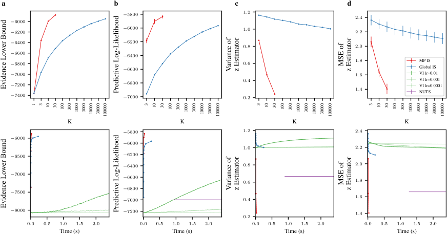
Figure 1: Results obtained in the MovieLens model. Columns a–c show the evidence lower bound, predictive log-likelihood and variance in the estimator of $\mathbf{z}_{m}$ using the true MovieLens100K data. Column d shows the mean squared error in the estimator of $\mathbf{z}_{m}$ when the data is sampled from the model and thus the true value of $\mathbf{z}_{m}$ is known. The error bars in the top-row represent the standard-deviation across different dataset splits.

Computing conditional distributions for importance sampling. A common alternative to importance weighting is importance sampling. In importance sampling, we rewrite the usual estimates of the expectations in terms of a distribution over indices, $\operatorname{P}\left(\mathbf{k}\right)$,

$$m_{\textrm{MP}}(z) =\sum_{\mathbf{k}\in\mathcal{K}^{n}}\operatorname{P}\left(\mathbf{k}\right)m(z^{\mathbf{k}})$$ (38)

where

$$\operatorname{P}\left(\mathbf{k}\right) =\frac{1}{K^{n}}\frac{1}{\mathcal{P}_{\textrm{MP}}(z)}r_{\mathbf{k}}(z)$$ (39)

We can obtain (approximate) posterior samples, $z^{\mathbf{k}}$, by sampling $\mathbf{k}$ from $\operatorname{P}\left(\mathbf{k}\right)$. However, sampling from $\operatorname{P}\left(\mathbf{k}\right)$ is difficult in our context, as there are $K^{n}$ possible settings of $\mathbf{k}$, so we cannot explicitly compute the full distribution. Instead, we need to factorise the distribution in some way, and iteratively sample (e.g. we sample $k_{1}$ from $\operatorname{P}\left(k_{1}\right)$ then sample $k_{2}$ from $\operatorname{P}\left(k_{2}\middle|k_{1}\right)$ etc.) However, this raises a question: how should we factorise the distribution over $\mathbf{k}$? This is a difficult problem in the probabilistic programming setting, because we need a factorisation that is always valid, and at the same time, has as few indices in each term as possible, to ensure that the computations remain efficient. By substituting Eq. (20) into Eq. (38),

$$\operatorname{P}\left(\mathbf{k}\right) =\frac{1}{K^{n}}\frac{1}{\mathcal{P}_{\textrm{MP}}(z)}f^{x}_{\mathbf{k}_{{\textrm{pa}\left(x\right)}}}(z)\prod_{i}f^{i}_{k_{i},\mathbf{k}_{\textrm{pa}\left(i\right)}}(z)$$ (40)

we can see that one valid factorisation follows the factorisation of the generative model. This is particularly useful, as it is guaranteed to be a valid factorisation, likely to be small (often minimal) and it is easy for us to extract. Formally, we use,

$$\operatorname{P}\left(\mathbf{k}\right) =\prod_{i}\operatorname{P}\left(k_{i}\middle|\mathbf{k}_{{\textrm{pa}\left(i\right)}}\right)$$ (41)

where

$$\mathbf{k}_{\textrm{pa}\left(i\right)} =\left(k_{j}\text{ for all }j\in{\textrm{pa}\left(i\right)}\right)$$ (42)

where, remember ${\textrm{pa}\left(i\right)}$ is the set of indices of parents of the $i$th latent variable under the generative model, and $\mathbf{k}_{\textrm{pa}\left(i\right)}$ is the value of $k$ for each of those parents. Note that this quantity is similar to the ”backward kernels” in the SMC literature (Del Moral, Doucet, and Jasra 2006), what’s different is our approach to computing the quantity, using the source-term trick to avoid the need for explicit backward traversals. Now, we have the problem of computing the conditionals, $\operatorname{P}\left(k_{i}\middle|\mathbf{k}_{{\textrm{pa}\left(i\right)}}\right)$. We can compute the conditionals from the marginals using Bayes theorem,

$$\operatorname{P}\left(k_{i}\middle|\mathbf{k}_{{\textrm{pa}\left(i\right)}}\right) =\frac{\operatorname{P}\left(k_{i},\mathbf{k}_{{\textrm{pa}\left(i\right)}}\right)}{\sum_{k^{\prime}_{i}}\operatorname{P}\left(k^{\prime}_{i},\mathbf{k}_{{\textrm{pa}\left(i\right)}}\right)}$$ (43)

where

$$\operatorname{P}\left(k_{i},\mathbf{k}_{{\textrm{pa}\left(i\right)}}\right) =\sum_{\mathbf{k}/(k_{i},\mathbf{k}_{{\textrm{pa}\left(i\right)}})}\operatorname{P}\left(\mathbf{k}\right)$$ (44)

Again, we can compute these marginals efficiently by differentiating a modified estimate of the marginal likelihood. This time, we take a tensor-valued $\mathbf{J}\in\mathbb{R}^{K^{1+\left\lvert{\textrm{pa}\left(i\right)}\right\rvert}}$, where remember $\left\lvert{\textrm{pa}\left(i\right)}\right\rvert$ is the number of parents of the $i$th latent variable under the generative model.

$$\mathcal{P}_{\textrm{MP}}^{\text{samp}}(z,\mathbf{J}) =\frac{1}{K^{n}}\sum_{\mathbf{k}}\frac{\operatorname{P}\left(x,z^{\mathbf{k}}\right)}{{\operatorname{Q}}\left(z^{\mathbf{k}}\right)}e^{J_{k_{i},\mathbf{k}_{{\textrm{pa}\left(i\right)}}}}$$ (45)

As usual, we differentiate with respect to $\mathbf{J}$ at $\mathbf{J}=\mathbf{0}$, letting

$$\nabla_{\mathcal{P}_{\textrm{MP}}^{\text{samp}}}=\left.\frac{\partial}{\partial J_{k^{\prime}_{i},\mathbf{k}^{\prime}_{\textrm{pa}\left(i\right)}}}\right\rvert_{\mathbf{J}=\mathbf{0}}\log\mathcal{P}_{\textrm{MP}}^{\text{samp}}(z,\mathbf{J})$$ (46)

then

$$\nabla_{\mathcal{P}_{\textrm{MP}}^{\text{samp}}}=\frac{\tfrac{1}{K^{n}}\sum_{\mathbf{k}}r_{\mathbf{k}}(z)\delta_{(k_{i},\mathbf{k}_{{\textrm{pa}\left(i\right)}}),(k^{\prime}_{i},\mathbf{k}^{\prime}_{{\textrm{pa}\left(i\right)}})}}{\mathcal{P}_{\textrm{MP}}(z)}$$ (47)

Here, $\delta_{(k_{i},\mathbf{k}_{{\textrm{pa}\left(i\right)}}),(k^{\prime}_{i},\mathbf{k}^{\prime}_{{\textrm{pa}\left(i\right)}})}$ is a generalisation of the Kronecker delta. It is $1$ when all the indices match (i.e. $k_{i}=k_{i}^{\prime}$, and $\mathbf{k}_{{\textrm{pa}\left(i\right)}}=\mathbf{k}^{\prime}_{{\textrm{pa}\left(i\right)}}$) and zero otherwise. These turn out to be precisely the marginals in Eq. (43),

$$\begin{split}\nabla_{\mathcal{P}_{\textrm{MP}}^{\text{samp}}}&=\frac{\tfrac{1}{K^{n}}\sum_{\mathbf{k}/(k_{i},\mathbf{k}_{{\textrm{pa}\left(i\right)}})}r_{\mathbf{k}}(z)}{\mathcal{P}_{\textrm{MP}}(z)}\\ &=\sum_{\mathbf{k}/(k_{i},\mathbf{k}_{{\textrm{pa}\left(i\right)}})}\operatorname{P}\left(\mathbf{k}\right)=\operatorname{P}\left(k_{i},\mathbf{k}_{{\textrm{pa}\left(i\right)}}\right).\end{split}$$ (48)

Experiments

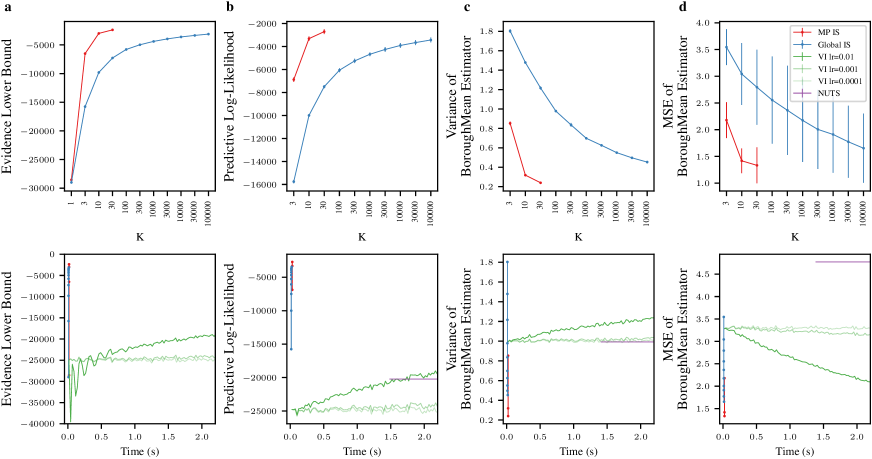
Figure 2: Results analogous to those in Fig. 1 for a different dataset: NYC Bus Breakdown. a–c are based on real data. c gives the variance in the mean estimate of $\mathrm{IdMean}_{mj}$ across runs. d gives the mean squared error between the mean estimate and the true value of $\mathrm{IdMean}_{mj}$ on simulated data.

We provide empirical results comparing the global and massively parallel importance weighting/sampling methods, as well as VI and HMC baselines. We considered two datasets: MovieLens100K (Fig. 1) and NYC Bus Breakdown (Fig. 2). MovieLens100K (Harper and Konstan 2015) contains 100k ratings of $N{=}1682$ films from among $M{=}943$ users. NYC Bus Breakdown describes the length of around 150,000 delays to New York school bus journeys, segregated by year, borough, bus company and journey type. We use hierarchical probabilistic graphical models for these datasets, which are described in more detail in Appendix section Experimental Datasets And Models.

For global and massively parallel importance sampling, we use the prior as a proposal. For VI, we used a factorised approximate posterior and optimized using Adam with learning rates ranging from $10^{-2}$ to $10^{-4}$ (learning rates faster than $10^{-2}$ were unstable). For HMC, we used the NUTS (Hoffman, Gelman et al. 2014) implementation from PyMC (Salvatier, Wiecki, and Fonnesbeck 2016).

We consider four quantities in Fig. 1 and Fig. 2. We begin by looking at the ELBO (Fig. 1a,2a). While massively parallel estimates of the ELBO can be computed using previous methods (e.g. Heap and Laurence 2023), it is nonetheless useful as it is a good measure of the quality of our approximate posteriors (as the ELBO can be written as the sum of the marginal likelihood and the KL-divergence between the true and approximate posterior Jordan et al. 1999; Kingma, Welling et al. 2019). Next, we plot the predictive log-likelihood, based on posterior samples obtained using the approach in the Methods section. In both of these plots, we see dramatic improvements against standard “global” importance sampling for a fixed $K$ (top row), and for a fixed time against other baselines such as VI and HMC (bottom row). Finally, we consider the quality of the posterior moment estimates computed using the approach in the Methods section. In particular we consider two measures of the quality of our posterior mean estimator. First, we consider the variance of the estimator (Fig. 1c,2c); in the ideal case, when we have exactly computed the posterior mean, this variance should be zero. While this variance can be zero in other cases (e.g. when the mean estimator always returns a constant), it does provide a lower-bound on the expected squared error between the estimator and the true value. Second, we directly considered the MSE between our posterior mean estimator and the true latent variable (Fig. 1d,2d). However, this quantity requires us to know the true value for the latent variable, which requires us to generate data from the model (we only generated data for d, columns a–c use real data). Again, in both of these cases, we see dramatic improvements for massively parallel against standard “global” importance sampling for a fixed $K$ (top row), and for a fixed time against other methods such as VI and HMC (bottom row).

Note the extremely poor performance of VI and HMC is because these are iterative methods that take many steps, and hence a long time to reach good performance. HMC is especially problematic on these short timescales, because it needs many gradient steps before it returns even a single posterior sample (and this is ignoring burn-in and adaptation phases). In contrast, importance sampling gets a reasonable answer much more quickly, as it just a single, non-iterative computation.

Conclusion and Limitations

We gave a new and far simpler method for computing posterior moments, marginals and samples in massively parallel importance sampling based on differentiating a slightly modified marginal likelihood estimator.

The method has limitations, in that while it is considerably more effective than e.g. VI, HMC and global importance sampling, it is more complex. Additionally, at least a naive implementation may be quite costly in terms of memory consumption, limiting how the number of importance samples we can draw for each variable. That said, it should be possible to eliminate almost all of this overhead by careful optimizations to avoid allocating large intermediate tensors, following the strategy in KeOps (Charlier et al. 2021).

Using autodiff to estimate posterior moments, marginals and samples
(Supplementary Material)

Appendix A Derivations

Global Importance Sampling

Here, we give the derivation for standard global importance sampling. Ideally we would compute moments using the true posterior, $\operatorname{P}\left(z|x\right)$,

$$m_{\textrm{post}} =\mathrm{E}_{\operatorname{P}\left(z^{k}|x\right)}\left[m(z^{k})\right].$$ (49)

However, the true posterior is not known. Instead, we write down the moment under the true posterior as an integral,

$$m_{\textrm{post}} =\int dz^{k}\operatorname{P}\left(z^{k}|x\right)m(z^{k}).$$ (50)

Next, we multiply the integrand by $$1={\operatorname{Q}}\left(z^{k}\right)/{\operatorname{Q}}\left(z^{k}\right)$$,

$$m_{\textrm{post}} =\int dz^{k}{\operatorname{Q}}\left(z^{k}\right)\frac{\operatorname{P}\left(z^{k}|x\right)}{{\operatorname{Q}}\left(z^{k}\right)}m(z^{k}).$$ (51)

Next, the integral can be written as an expectation,

$$m_{\textrm{post}} =\mathrm{E}_{{\operatorname{Q}}\left(z^{k}\right)}\left[\frac{\operatorname{P}\left(z^{k}|x\right)}{{\operatorname{Q}}\left(z^{k}\right)}m(z^{k})\right].$$ (52)

It looks like we should be able to estimate $m_{\textrm{post}}$ by sampling from our approximate posterior, ${\operatorname{Q}}\left(z^{k}\right)$. However, this is not yet possible, as we are not able to compute the true posterior, $\operatorname{P}\left(z^{k}|x\right)$. We might consider using Bayes theorem,

$$\operatorname{P}\left(z^{k}|x\right) =\frac{\operatorname{P}\left(z^{k},x\right)}{\operatorname{P}\left(x\right)},$$ (53)

but this requires computing an intractable normalizing constant,

$$\operatorname{P}\left(x\right) =\int dz^{k}\operatorname{P}\left(z^{k},x\right).$$ (54)

Instead, we use an unbiased, importance-sampled estimate of the normalizing constant, $\mathcal{P}_{\textrm{global}}(z)$ (Eq. 7). Burda, Grosse, and Salakhutdinov (2015) showed that in the limit as $K\rightarrow\infty$, $\mathcal{P}_{\textrm{global}}(z)$ approaches $\operatorname{P}\left(x\right)$. Using this estimate of the marginal likelihood our moment estimate becomes,

$$m_{\textrm{global}} =\mathrm{E}_{{\operatorname{Q}}\left(z^{k}\right)}\left[\frac{\frac{\operatorname{P}\left(z^{k},x\right)}{{\operatorname{Q}}\left(z^{k}\right)}}{\mathcal{P}_{\textrm{global}}(z)}m(z^{k})\right].$$ (55)

Using $r_{k}(z)$ (Eq. 6), we can write this expression as,

$$m_{\textrm{global}} =\mathrm{E}_{{\operatorname{Q}}_{\phi}\left(z\right)}\left[\frac{r_{k}(z)}{\mathcal{P}_{\textrm{global}}(z)}m(z^{k})\right].$$ (56)

The approximate posterior and generative probabilities are the same for different values of $k$, so we can average over $k$, which gives Eq. (5) in the main text.

Massively Parallel Importance Sampling

Inspired by the global importance sampling derivation, we consider massively parallel importance sampling. In the global importance sampling derivation, the key idea was to show that the estimator was unbiased for each of the $K$ samples, $z^{k}$, in which case the average over all $K$ samples is also unbiased. In massively parallel importance sampling, we use the same idea, except that we now have $K^{n}$ samples, denoted $z^{\mathbf{k}}$. As before,

$$m_{\textrm{post}} =\mathrm{E}_{\operatorname{P}\left(z^{\mathbf{k}}|x\right)}\left[m(z^{\mathbf{k}})\right]=\int dz^{\mathbf{k}}\operatorname{P}\left(z^{\mathbf{k}}|x\right)m(z^{\mathbf{k}}).$$ (57)

Again, we multiply and divide by the approximate posterior for $$z^{\mathbf{k}} \prod_{i}{\operatorname{Q}}\left(z_{i}^{k_{i}}\middle|z_{\textrm{qa}\left(i\right)}\right)$$. In the massively parallel setting, we specifically use ,

$$m_{\textrm{post}} =\int dz^{\mathbf{k}}\left(\prod_{i}{\operatorname{Q}}\left(z_{i}^{k_{i}}\middle|z_{\textrm{qa}\left(i\right)}\right)\right)\frac{\operatorname{P}\left(z^{\mathbf{k}}|x\right)}{\prod_{i}{\operatorname{Q}}\left(z_{i}^{k_{i}}\middle|z_{\textrm{qa}\left(i\right)}\right)}m(z^{\mathbf{k}}).$$ (58)

Overall, our goal is to convert the integral over the indexed latent variables in Eq. (58) into an integral over the full latent space, $z$, so that it can be written as an expectation over the proposal, ${\operatorname{Q}}\left(z\right)$. To do that, we need to introduce the concept of non-indexed latent variables. These are all samples of the latent variables, except for the “indexed”, or $k$th sample. For the $i$th latent variable, the non-indexed samples are,

$$z_{i}^{/k_{i}} =\left(z_{i}^{1},\dotsc,z_{i}^{k_{i}-1},z_{i}^{k_{i}+1},\dotsc,z_{i}^{K}\right)\in\mathcal{Z}_{i}^{K-1}.$$ (59)

We can also succinctly write the non-indexed samples of all latent variables as,

$$z^{/\mathbf{k}} =\left(z_{1}^{/k_{1}},z_{2}^{/k_{2}},\dotsc,z_{n}^{/k_{n}}\right)\in\mathcal{Z}^{K-1}.$$ (60)

The joint distribution over the non-indexed latent variables, conditioned on the indexed latent variables integrates to $1$,

$$1 =\int dz^{/\mathbf{k}}\prod_{i}{\operatorname{Q}}\left(z_{i}^{/k_{i}}\middle|z_{i}^{k_{i}},z_{\textrm{qa}\left(i\right)}\right),$$ (61)

We use this to multiply the integrand in Eq. (58),

$$m_{\textrm{post}} =\int dz^{\mathbf{k}}\left(\prod_{i}{\operatorname{Q}}\left(z_{i}^{k_{i}}\middle|z_{\textrm{qa}\left(i\right)}\right)\right)\frac{\operatorname{P}\left(z^{\mathbf{k}}|x\right)}{\prod_{i}{\operatorname{Q}}\left(z_{i}^{k_{i}}\middle|z_{\textrm{qa}\left(i\right)}\right)}m(z^{\mathbf{k}})\int dz^{/\mathbf{k}}\prod_{i}{\operatorname{Q}}\left(z_{i}^{/k_{i}}\middle|z_{i}^{k_{i}},z_{\textrm{qa}\left(i\right)}\right).$$ (62)

Next, we merge the integrals over over $z^{\mathbf{k}}$ and $z^{/\mathbf{k}}$ to form one integral over $z$,

$$m_{\textrm{post}} =\int dz\;{\operatorname{Q}}\left(z\right)\frac{\operatorname{P}\left(z^{\mathbf{k}}|x\right)}{\prod_{i}{\operatorname{Q}}\left(z_{i}^{k_{i}}\middle|z_{\textrm{qa}\left(i\right)}\right)}m(z^{\mathbf{k}}).$$ (63)

This integral can be written as an expectation,

$$m_{\textrm{post}} =\mathrm{E}_{{\operatorname{Q}}\left(z\right)}\left[\frac{\operatorname{P}\left(z^{\mathbf{k}}|x\right)}{\prod_{i}{\operatorname{Q}}\left(z_{i}^{k_{i}}|z_{{\textrm{pa}\left(i\right)}}\right)}m(z^{\mathbf{k}})\right].$$ (64)

As in the derivation for global importance sampling, it looks like we might be able to estimate this by sampling from ${\operatorname{Q}}\left(z|x\right)$, but this does not yet work as we do not yet have a form for the posterior. Again, we could compute the posterior using Bayes theorem,

$$\operatorname{P}\left(z^{\mathbf{k}}|x\right) =\tfrac{\operatorname{P}\left(z^{\mathbf{k}},x\right)}{\operatorname{P}\left(x\right)},$$ (65)

but we cannot compute the model evidence,

$$\operatorname{P}_{\theta}\left(x\right)=\int dz^{\mathbf{k}}\operatorname{P}_{\theta}\left(z^{\mathbf{k}},x\right).$$ (66)

As in the global importance sampling section, we instead use an estimate of the marginal likelihood. Here, we use a massively parallel estimate, $\mathcal{P}_{\textrm{MP}}(z)$,

$$m_{\textrm{MP}} =\mathrm{E}_{{\operatorname{Q}}\left(z|x\right)}\left[\frac{\frac{\operatorname{P}\left(z^{\mathbf{k}},x\right)}{\prod_{i}{\operatorname{Q}}\left(z_{i}^{k_{i}}|z_{{\textrm{pa}\left(i\right)}}\right)}}{\mathcal{P}_{\textrm{MP}}(z)}m(z^{\mathbf{k}})\right].$$ (67)

Again, we use $r_{\mathbf{k}}(z)$ (Eq. 18),

$$m_{\textrm{MP}} =\mathrm{E}_{{\operatorname{Q}}\left(z\right)}\left[\frac{r_{\mathbf{k}}(z)}{\mathcal{P}_{\textrm{MP}}(z)}m(z^{\mathbf{k}})\right].$$ (68)

So the value for a single set of latent variables, $z^{\mathbf{k}}$, has the right expectation. Thus, averaging over all $K^{n}$ settings of $\mathbf{k}$, we get the unbiased estimator in the main text, (Eq. 24).

Appendix B Algorithms

Algorithm 1 Expectations using Source Trick

Data $x$, Generative Model $\mathrm{P}(\mathbf{x}|z)$, Prior $\mathrm{P}(\mathbf{z})$, Proposal $\mathrm{Q}_{\mathrm{MP}}$, $K\geq 1$, function whose expectation we want to compute $m(z^{\mathbf{k}})$

for $i\leftarrow 1$ to $n$ do

     Sample $z_{i}\sim{\operatorname{Q}}_{\textrm{MP}}\left(z_{i}\middle|z_{j}\text{ for all }j\in{\textrm{qa}\left(i\right)}\right)$

     $z\leftarrow\{z_{1},...,z_{i-1}\}\cup z_{i}$

     $f^{i}_{k_{i},\mathbf{k}_{{\textrm{pa}\left(i\right)}}}(z)\leftarrow\frac{\operatorname{P}\left(z^{k_{i}}_{i}\middle|z_{j}^{k_{j}}\text{ for all }j\in{\textrm{pa}\left(i\right)}\right)}{{\operatorname{Q}}_{\textrm{MP}}\left(z_{i}^{k_{i}}|x,z_{j}\text{ for all }j\in{\textrm{qa}\left(i\right)}\right)}$

end for

$f^{x}_{\mathbf{k}_{{\textrm{pa}\left(x\right)}}}(z)\leftarrow\operatorname{P}\left(x\middle|z_{j}^{k_{j}}\text{ for all }j\in{\textrm{pa}\left(x\right)}\right)$

$r_{\mathbf{k}}(z)\leftarrow f^{x}_{\mathbf{k}_{{\textrm{pa}\left(x\right)}}}(z)\prod_{i}f^{i}_{k_{i},\mathbf{k}_{{\textrm{pa}\left(i\right)}}}(z)$

$J\leftarrow 0$

$\mathcal{P}_{\textrm{MP}}^{\text{exp}}(z,J)\leftarrow\tfrac{1}{K^{n}}\sum_{\mathbf{k}^{n}}r_{\mathbf{k}}(z)e^{Jm(z^{\mathbf{k}})}$

$m_{\textrm{MP}}(z)\leftarrow\left.\frac{\partial}{\partial J}\right\rvert_{J=0}\log\mathcal{P}_{\textrm{MP}}^{\text{exp}}(z,J)$

Algorithm 2 Marginal importance weights using Source Trick

Data $x$, Generative Model $\mathrm{P}(\mathbf{x}|z)$, Prior $\mathrm{P}(\mathbf{z})$, Proposal $\mathrm{Q}_{\mathrm{MP}}$, $K\geq 1$, index of latent for which to calculate weight: $i$

for $i\leftarrow 1$ to $n$ do

     Sample $z_{i}\sim{\operatorname{Q}}_{\textrm{MP}}\left(z_{i}\middle|z_{j}\text{ for all }j\in{\textrm{qa}\left(i\right)}\right)$

     $z\leftarrow\{z_{1},...,z_{i-1}\}\cup z_{i}$

     $f^{i}_{k_{i},\mathbf{k}_{{\textrm{pa}\left(i\right)}}}(z)\leftarrow\frac{\operatorname{P}\left(z^{k_{i}}_{i}\middle|z_{j}^{k_{j}}\text{ for all }j\in{\textrm{pa}\left(i\right)}\right)}{{\operatorname{Q}}_{\textrm{MP}}\left(z_{i}^{k_{i}}|x,z_{j}\text{ for all }j\in{\textrm{qa}\left(i\right)}\right)}$

end for

$f^{x}_{\mathbf{k}_{{\textrm{pa}\left(x\right)}}}(z)\leftarrow\operatorname{P}\left(x\middle|z_{j}^{k_{j}}\text{ for all }j\in{\textrm{pa}\left(x\right)}\right)$

$r_{\mathbf{k}}(z)\leftarrow f^{x}_{\mathbf{k}_{{\textrm{pa}\left(x\right)}}}(z)\prod_{i}f^{i}_{k_{i},\mathbf{k}_{{\textrm{pa}\left(i\right)}}}(z)$

$\mathbf{J}\leftarrow\mathbf{0}\in\mathbb{R}^{K}$

$\mathcal{P}_{\textrm{MP}}^{\text{marg}}(z,\mathbf{J})\leftarrow\tfrac{1}{K^{n}}\sum_{\mathbf{k}^{n}}r_{\mathbf{k}}(z)e^{J_{k_{i}}}$

$w^{i}_{k_{i}}\leftarrow\left.\frac{\partial}{\partial J_{k_{i}}}\right\rvert_{J=0}\log\mathcal{P}_{\textrm{MP}}^{\text{marg}}(z,\mathbf{J})$

Algorithm 3 Conditional distributions using Source Trick

Data $x$, Generative Model $\mathrm{P}(\mathbf{x}|z)$, Prior $\mathrm{P}(\mathbf{z})$, Proposal $\mathrm{Q}_{\mathrm{MP}}$, $K\geq 1$, index of latent for which to compute conditional distribution: $i$

for $i\leftarrow 1$ to $n$ do

     Sample $z_{i}\sim{\operatorname{Q}}_{\textrm{MP}}\left(z_{i}\middle|z_{j}\text{ for all }j\in{\textrm{qa}\left(i\right)}\right)$

     $z\leftarrow\{z_{1},...,z_{i-1}\}\cup z_{i}$

     $f^{i}_{k_{i},\mathbf{k}_{{\textrm{pa}\left(i\right)}}}(z)\leftarrow\frac{\operatorname{P}\left(z^{k_{i}}_{i}\middle|z_{j}^{k_{j}}\text{ for all }j\in{\textrm{pa}\left(i\right)}\right)}{{\operatorname{Q}}_{\textrm{MP}}\left(z_{i}^{k_{i}}|x,z_{j}\text{ for all }j\in{\textrm{qa}\left(i\right)}\right)}$

end for

$f^{x}_{\mathbf{k}_{{\textrm{pa}\left(x\right)}}}(z)\leftarrow\operatorname{P}\left(x\middle|z_{j}^{k_{j}}\text{ for all }j\in{\textrm{pa}\left(x\right)}\right)$

$\mathbf{J}\leftarrow\mathbf{0}\in\mathbb{R}^{K^{1+|\text{pa}(i)|}}$

$r_{\mathbf{k}}(z)\leftarrow f^{x}_{\mathbf{k}_{{\textrm{pa}\left(x\right)}}}(z)\prod_{i}f^{i}_{k_{i},\mathbf{k}_{{\textrm{pa}\left(i\right)}}}(z)$

$\mathcal{P}_{\textrm{MP}}^{\text{samp}}(z,\mathbf{J})\leftarrow\frac{1}{K^{n}}\sum_{\mathbf{k}}\frac{\operatorname{P}\left(x,z^{\mathbf{k}}\right)}{{\operatorname{Q}}\left(z^{\mathbf{k}}\right)}e^{J_{k_{i},\mathbf{k}_{{\textrm{pa}\left(i\right)}}}}$

$\operatorname{P}\left(k_{i},\mathbf{k}_{{\textrm{pa}\left(i\right)}}\right)\leftarrow\left.\frac{\partial}{\partial J_{k_{i},\mathbf{k}_{\textrm{pa}\left(i\right)}}}\right\rvert_{\mathbf{J}=\mathbf{0}}\log\mathcal{P}_{\textrm{MP}}^{\text{samp}}(z,\mathbf{J})$

Appendix C Experimental Datasets And Models

MovieLens Dataset

The MovieLens100K (Harper and Konstan 2015) dataset contains 100k ratings of $N{=}1682$ films from among $M{=}943$ users. The original user ratings run from 0 to 5. Following Geffner and Domke (2022), we binarise the ratings into just likes/dislikes, by taking user-ratings of $\{0,1,2,3\}$ as a binarised-rating of $0$ (dislikes) and user-ratings of $\{4,5\}$ as a binarised-rating of $1$ (likes). We assume binarised ratings of 0 for films which users have not previously rated.

The probabilistic graphical model is given in Fig 3. We use $n$ to index films, and $m$ to index users. Each film has a known feature vector, $\mathbf{x}_{n}$, while each user has a latent weight-vector, $\mathbf{z}_{m}$, of the same length, describing whether or not they like any given feature. There are 18 features, indicating which genre tags the film has (Action, Adventure, Animation, Childrens,…). Each film may have more than one tag. The probability of the user liking a film is given by taking the dot-product of the film’s feature vector with the latent weight-vector, and applying a sigmoid ($\sigma(\cdot)$) (final line)

$$\boldsymbol{\mu} \sim\mathcal{N}(\mathbf{0}_{18},\tfrac{1}{4}\mathbf{I})$$

$$\boldsymbol{\psi} \sim\mathcal{N}(\mathbf{0}_{18},\tfrac{1}{4}\mathbf{I})$$

$$\mathbf{z}_{m} \sim\mathcal{N}(\boldsymbol{\mu},\exp(\boldsymbol{\psi})\mathbf{I}),\ m=1,\dotsc,M$$

$$\mathrm{Rating}_{mn} \sim\operatorname{Bernoulli}(\sigma(\mathbf{z}_{m}^{\intercal}\mathbf{x}_{n})),\ n=1,\dotsc,N$$ (69)

Additionally, we have latent vectors for the global mean, $\boldsymbol{\mu}$, and variance, $\boldsymbol{\psi}$, of the weight vectors. We use a random subset of $N=20$ films and $M=450$ users for our experiment to ensure high levels of uncertainty. We use equally sized but disjoint subset of users held aside for calculation of the predictive log-likelihood. In Fig. 1c,d we consider the variance and MSE of estimators of $\mathbf{z}_{m}$.

Figure 3: Graphical model for the MovieLens dataset

Bus Delay Dataset

In our second experiment, we model the length of delays to New York school bus journeys, working with a dataset supplied by the City of New York (DOE 2023). Our goal is to predict the length of a delay, based on the year, $y$, borough, $b$, bus company, $c$ and journey type, $j$. Specifically, our data includes the years $2015-2022$ inclusive and covers the five New York boroughs (Brooklyn, Manhatten, The Bronx, Queens, Staten Island) as well as some surrounding areas (Nassau County, New Jersey, Connecticut, Rockland County, Westchester). There are 57 bus companies, and 6 different journey types (e.g. pre-K/elementary school route, general education AM/PM route etc.) We take $I=60$ delayed buses in each borough and year, and take $Y=3$ years and $B=3$ boroughs. We then split along the $I$ dimension to get two equally sized train and test sets. Thus, each delay is uniquely identified by the year, $y$, the borough, $b$, and the index, $i$, giving $\mathrm{delay}_{ybi}$ The delays are recorded as an integer number of minutes and we discard any entries greater than $130$ minutes.

We have a hierarchical latent variable model describing the impact of each of the features (year, borough, bus company and journey type) on the length of delays. Specifically, the integer delay is modelled with a Negative Binomial distribution, with fixed total count of 130, as we discard entries with delays longer than this. The expected delay length is controlled by a logits latent variable, $\mathrm{logits}_{ybi}$, with one logits for each delayed bus. The logits is a sum of three terms: one for the borough and year jointly, one for the bus company and one for the journey type. Each of these three terms is themselves a latent variable that must be inferred.

First, we have a term for the year and borough, $\mathrm{YearBoroughWeight}_{yb}$, which has a hierarchical prior. Specifically, we begin by sampling a global mean and variance, $\mathrm{GlobalMean}$ and $\mathrm{GlobalVariance}$. Then for each year, we use $\mathrm{GlobalMean}$ and $\mathrm{GlobalVariance}$ to sample a mean for each year, $\mathrm{YearMean}_{y}$. Additionally, we sample a variance for each borough, $\mathrm{BoroughVariance}_{b}$. Then we sample a $\mathrm{YearBoroughWeight}_{yb}$ from a Gaussian distribution with a year-dependent mean, $\mathrm{YearMean}_{y}$, and a borough-dependent variance, $\mathrm{BoroughVariance}_{b}$.

Next, the weights for the bus company and journey type are very similar. Specifically, we have one latent weight for each bus company, $\mathrm{CompanyWeight}_{c}$, with $c\in\{1,\dotsc,57\}$, and for each journey type, $\mathrm{JourneyTypeWeight}_{j}$, with $j\in\{1,\dotsc,6\}$. We have a table identifying the bus company, $b_{ybi}$, and journey type, $j_{ybi}$, for each delayed bus journey (remember that a particular delayed bus journey is uniquely identified by the year, $y$, borough, $b$ and index $i$). In $\mathrm{logits_{ybi}}$ we use these tables to pick out the right company and journey type weight for that particular delayed bus journey, $\mathrm{CompanyWeight}_{c_{ybi}}$ and $\mathrm{JourneyTypeWeight}_{c_{ybi}}$. The final generative model is,

$$\begin{split}\mathrm{GlobalVariance}&\sim\mathcal{N}(0,10^{-4})\\ \mathrm{GlobalMean}&\sim\mathcal{N}(0,10^{-4})\\ \mathrm{YearMean}_{y}&\sim\mathcal{N}(\mathrm{GlobalMean},\exp(\mathrm{GlobalVariance})),\ y\in\{1,...,Y\}\\ \mathrm{BoroughVariance}_{b}&\sim\mathcal{N}(0,0.25),\ b\in\{1,...,B\}\\ \mathrm{YearBoroughWeight}_{yb}&\sim\mathcal{N}(\mathrm{YearMean}_{y},\exp(\mathrm{BoroughVariance}_{b})),\\ \mathrm{WeightVariance}&\sim\mathcal{N}(0,10^{-4}),\\ \mathrm{CompanyWeight}_{c}&\sim\mathcal{N}(0,\exp(\mathrm{WeightVariance})),\ c\in\{1,...,C\}\\ \mathrm{JourneyTypeWeight}_{j}&\sim\mathcal{N}(0,\exp(\mathrm{WeightVariance})),\ j\in\{1,...,J\}\\ \mathrm{logits}_{ybi}&=\mathrm{YearBoroughWeight}_{yb}+\mathrm{CompanyWeight}_{c_{ybi}}+\mathrm{JourneyTypeWeight}_{j_{ybi}}\\ \mathrm{delay}_{ybi}&\sim\mathrm{NegativeBinomial}(\mathrm{total\ count}=130,\mathrm{logits}_{ybi}),\end{split}$$ (70)

and the graphical model is given in Fig. 4

Figure 4: Graphical model for the NYC Bus Breakdown dataset

Experiment Details

We ran all experiments on an 80GB NVIDIA A100 GPU and averaged the results over three different dataset splits generated using different random seeds. On each dataset split, the MovieLens experiments required a maximum 26.9 GB of memory at any one time. For the NYC Bus Breakdown experiments this value was 0.9 GB. For each experiment using a single dataset split, we used global IS, MP IS, VI and HMC methods to obtain (for each value of $K$ in the IS methods, or each iteration of VI/HMC) 1000 values of the ELBO, predictive log-likelihood (on a test set that was disjoint from the training set), and posterior mean estimates for each latent variable in the model. These 1000 values were averaged for the ELBO and predictive log-likelihood, whilst the 1000 mean estimates were used to calculate mean squared error or variance per variable, based on whether the observed data had been sampled from the model itself—in which case the true variable values were known—or not. We present error bars in the top rows of Fig. 1 and Fig. 2 representing the standard deviation over the three dataset splits.

For VI, we optimize our approximate posterior using Adam with learning rates of $10^{-2},10^{-3}$ and $10^{-4}$ (we found that learning rates faster than $10^{-2}$ were unstable), and ran 100 optimization steps for both for the MovieLens and Bus Breakdown models. For HMC, we ran the No U-Turn Sampler on our GPU using JAX (Bradbury et al. 2018) to obtain 10 consecutive samples after a single step with PyMC’s (Salvatier, Wiecki, and Fonnesbeck 2016) pre-tuning and with all other parameters set to their default values. We present results of the first 5 samples (not including the tuning sample) in order to align as best we can with the small time-scale of the IS methods.

References

- Aitchison (2019) Aitchison, L. 2019. Tensor Monte Carlo: particle methods for the GPU era. Advances in Neural Information Processing Systems, 32.
- Albarghouthi et al. (2017) Albarghouthi, A.; D’Antoni, L.; Drews, S.; and Nori, A. V. 2017. Fairsquare: probabilistic verification of program fairness. Proceedings of the ACM on Programming Languages, 1(OOPSLA): 1–30.
- Andrieu, Doucet, and Holenstein (2010) Andrieu, C.; Doucet, A.; and Holenstein, R. 2010. Particle markov chain monte carlo methods. Journal of the Royal Statistical Society: Series B (Statistical Methodology), 72(3): 269–342.
- Bidyuk and Dechter (2007) Bidyuk, B.; and Dechter, R. 2007. Cutset sampling for Bayesian networks. Journal of Artificial Intelligence Research, 28: 1–48.
- Bornschein and Bengio (2014) Bornschein, J.; and Bengio, Y. 2014. Reweighted wake-sleep. arXiv preprint arXiv:1406.2751.
- Bradbury et al. (2018) Bradbury, J.; Frostig, R.; Hawkins, P.; Johnson, M. J.; Leary, C.; Maclaurin, D.; Necula, G.; Paszke, A.; VanderPlas, J.; Wanderman-Milne, S.; and Zhang, Q. 2018. JAX: composable transformations of Python+NumPy programs.
- Burda, Grosse, and Salakhutdinov (2015) Burda, Y.; Grosse, R.; and Salakhutdinov, R. 2015. Importance weighted autoencoders. arXiv preprint arXiv:1509.00519.
- Charlier et al. (2021) Charlier, B.; Feydy, J.; Glaunès, J. A.; Collin, F.-D.; and Durif, G. 2021. Kernel Operations on the GPU, with Autodiff, without Memory Overflows. Journal of Machine Learning Research.
- Chatterjee and Diaconis (2018) Chatterjee, S.; and Diaconis, P. 2018. The sample size required in importance sampling. The Annals of Applied Probability, 28(2): 1099–1135.
- Claret et al. (2013) Claret, G.; Rajamani, S. K.; Nori, A. V.; Gordon, A. D.; and Borgström, J. 2013. Bayesian inference using data flow analysis. In Proceedings of the 2013 9th joint meeting on foundations of software engineering, 92–102.
- Corenflos, Chopin, and Särkkä (2022) Corenflos, A.; Chopin, N.; and Särkkä, S. 2022. De-Sequentialized Monte Carlo: a parallel-in-time particle smoother. arXiv preprint arXiv:2202.02264.
- Crucinio and Johansen (2023) Crucinio, F. R.; and Johansen, A. M. 2023. Properties of Marginal Sequential Monte Carlo Methods. ArXiv:2303.03498 [math, stat].
- Dawid (1992) Dawid, A. P. 1992. Applications of a general propagation algorithm for probabilistic expert systems. Statistics and computing, 2(1): 25–36.
- Dechter et al. (2018) Dechter, R.; Broka, F.; Kask, K.; and Ihler, A. 2018. Abstraction Sampling in Graphical Models. AAAI.
- Del Moral, Doucet, and Jasra (2006) Del Moral, P.; Doucet, A.; and Jasra, A. 2006. Sequential Monte Carlo Samplers. Journal of the Royal Statistical Society Series B: Statistical Methodology, 68(3): 411–436.
- DOE (2023) DOE. 2023. Bus Breakdown and Delays. url https://data.cityofnewyork.us/Transportation/Bus-Breakdown-and-Delays/ez4e-fazm Accessed on: 05.05.2023.
- Doucet, Johansen et al. (2009) Doucet, A.; Johansen, A. M.; et al. 2009. A tutorial on particle filtering and smoothing: Fifteen years later. Handbook of nonlinear filtering, 12(656-704): 3.
- Geffner and Domke (2022) Geffner, T.; and Domke, J. 2022. Variational Inference with Locally Enhanced Bounds for Hierarchical Models. arXiv preprint arXiv:2203.04432.
- Gehr, Misailovic, and Vechev (2016) Gehr, T.; Misailovic, S.; and Vechev, M. 2016. PSI: Exact symbolic inference for probabilistic programs. In International Conference on Computer Aided Verification, 62–83. Springer.
- Geldenhuys, Dwyer, and Visser (2012) Geldenhuys, J.; Dwyer, M. B.; and Visser, W. 2012. Probabilistic symbolic execution. In Proceedings of the 2012 International Symposium on Software Testing and Analysis, 166–176.
- Gogate and Dechter (2012) Gogate, V.; and Dechter, R. 2012. Importance sampling-based estimation over and/or search spaces for graphical models. Artificial Intelligence, 184: 38–77.
- Goodman and Stuhlmüller (2014) Goodman, N. D.; and Stuhlmüller, A. 2014. The design and implementation of probabilistic programming languages.
- Gordon, Salmond, and Smith (1993) Gordon, N. J.; Salmond, D. J.; and Smith, A. F. 1993. Novel approach to nonlinear/non-Gaussian Bayesian state estimation. In IEE proceedings F (radar and signal processing), volume 140, 107–113. IET.
- Harper and Konstan (2015) Harper, F. M.; and Konstan, J. A. 2015. The movielens datasets: History and context. Acm transactions on interactive intelligent systems (tiis), 5(4): 1–19.
- Heap and Laurence (2023) Heap, T.; and Laurence, A. 2023. Massively parallel reweighted wake-sleep. UAI.
- Hoffman, Gelman et al. (2014) Hoffman, M. D.; Gelman, A.; et al. 2014. The No-U-Turn sampler: adaptively setting path lengths in Hamiltonian Monte Carlo. J. Mach. Learn. Res., 15(1): 1593–1623.
- Holtzen, Van den Broeck, and Millstein (2020) Holtzen, S.; Van den Broeck, G.; and Millstein, T. 2020. Scaling exact inference for discrete probabilistic programs. Proceedings of the ACM on Programming Languages, 4(OOPSLA): 1–31.
- Jordan et al. (1999) Jordan, M. I.; Ghahramani, Z.; Jaakkola, T. S.; and Saul, L. K. 1999. An introduction to variational methods for graphical models. Machine learning, 37(2): 183–233.
- Kingma, Welling et al. (2019) Kingma, D. P.; Welling, M.; et al. 2019. An introduction to variational autoencoders. Foundations and Trends® in Machine Learning, 12(4): 307–392.
- Kuntz, Crucinio, and Johansen (2023) Kuntz, J.; Crucinio, F. R.; and Johansen, A. M. 2023. The divide-and-conquer sequential Monte Carlo algorithm: theoretical properties and limit theorems. ArXiv:2110.15782 [math, stat].
- Lai, Domke, and Sheldon (2022) Lai, J.; Domke, J.; and Sheldon, D. 2022. Variational Marginal Particle Filters. In International Conference on Artificial Intelligence and Statistics, 875–895. PMLR.
- Le et al. (2017) Le, T. A.; Igl, M.; Rainforth, T.; Jin, T.; and Wood, F. 2017. Auto-encoding sequential monte carlo. arXiv preprint arXiv:1705.10306.
- Le et al. (2020) Le, T. A.; Kosiorek, A. R.; Siddharth, N.; Teh, Y. W.; and Wood, F. 2020. Revisiting reweighted wake-sleep for models with stochastic control flow. In Uncertainty in Artificial Intelligence, 1039–1049. PMLR.
- Lindsten et al. (2017) Lindsten, F.; Johansen, A. M.; Naesseth, C. A.; Kirkpatrick, B.; Schön, T. B.; Aston, J.; and Bouchard-Côté, A. 2017. Divide-and-conquer with sequential Monte Carlo. Journal of Computational and Graphical Statistics, 26(2): 445–458.
- Maddison et al. (2017) Maddison, C. J.; Lawson, J.; Tucker, G.; Heess, N.; Norouzi, M.; Mnih, A.; Doucet, A.; and Teh, Y. 2017. Filtering variational objectives. Advances in Neural Information Processing Systems, 30.
- Naesseth et al. (2018) Naesseth, C.; Linderman, S.; Ranganath, R.; and Blei, D. 2018. Variational sequential monte carlo. In International conference on artificial intelligence and statistics, 968–977. PMLR.
- Narayanan et al. (2016) Narayanan, P.; Carette, J.; Romano, W.; Shan, C.-c.; and Zinkov, R. 2016. Probabilistic inference by program transformation in Hakaru (system description). In International Symposium on Functional and Logic Programming, 62–79. Springer.
- Obermeyer et al. (2019) Obermeyer, F.; Bingham, E.; Jankowiak, M.; Pradhan, N.; Chiu, J.; Rush, A.; and Goodman, N. 2019. Tensor variable elimination for plated factor graphs. In International Conference on Machine Learning, 4871–4880. PMLR.
- Pfeffer (2005) Pfeffer, A. 2005. The design and implementation of IBAL: A generalpurpose probabilistic programming language. In Harvard Univesity. Citeseer.
- Salvatier, Wiecki, and Fonnesbeck (2016) Salvatier, J.; Wiecki, T. V.; and Fonnesbeck, C. 2016. Probabilistic programming in Python using PyMC3. PeerJ Computer Science, 2: e55. Publisher: PeerJ Inc.
- Sankaranarayanan, Chakarov, and Gulwani (2013) Sankaranarayanan, S.; Chakarov, A.; and Gulwani, S. 2013. Static analysis for probabilistic programs: inferring whole program properties from finitely many paths. In Proceedings of the 34th ACM SIGPLAN conference on Programming language design and implementation, 447–458.
- Wang, Hoffmann, and Reps (2018) Wang, D.; Hoffmann, J.; and Reps, T. 2018. PMAF: an algebraic framework for static analysis of probabilistic programs. ACM SIGPLAN Notices, 53(4): 513–528.
- Weinberg (1995) Weinberg, S. 1995. The quantum theory of fields, volume 2. Cambridge university press.
- Zavatone-Veth et al. (2021) Zavatone-Veth, J.; Canatar, A.; Ruben, B.; and Pehlevan, C. 2021. Asymptotics of representation learning in finite Bayesian neural networks. Advances in neural information processing systems, 34: 24765–24777.