Polarization and third-order Hall effect in III-V semiconductor heterojunctions

Abstract

We study Berry connection polarizability (BCP) induced electric polarization and third-order Hall (TOH) effect in a two-dimensional electron/hole gas (2DEG/2DHG) with Rashba-Dresselhaus (RD) spin-orbit couplings in III-V semiconductor heterostructures. The electric polarization decreases with increase of the Fermi energy and is responsive to the electric field orientation in the presence of RD spin-orbit couplings for both the systems. We determine the BCP-induced TOH conductivity ($\chi_{\perp}^{\text{I}}$) along with the TOH conductivity associated with the band velocity ($\chi_{\perp}^{\text{II}}$). We find that the presence of an infinitesimal amount of Dresselhaus coupling in addition to the dominant Rashba coupling results in finite TOH responses. These conductivities vanish when the field is aligned with and/or orthogonal to the symmetry lines $k_{x}\pm k_{y}=0$ in both the systems. For typical system parameters in a 2DEG with $k$-linear RD interactions, the magnitude of $\chi_{\perp}^{\text{I}}$ is smaller than that of $\chi_{\perp}^{\text{II}}$. On the other hand, when both the SO couplings are comparable, $\chi_{\perp}^{\text{I}}$ shows a notable increase in magnitude, owing to the distinctive characteristics of BCP. The TOH conductivity of 2DEG remains unchanged when Rashba and Dresselhaus spin-orbit couplings are exchanged. For 2DHG with $k$-cubic RD interactions, $\chi_{\perp}^{\text{I},h}$ exhibits a larger magnitude compared to $\chi_{\perp}^{\text{II},h}$. Unlike the electron case, the BCP induced $\chi_{\perp}^{\text{I},h}$ alters under the exchange of spin-orbit coupling parameters, whereas $\chi_{\perp}^{\text{II},h}$ remains the same.

I Introduction

The discovery of the Hall effecthall in 1879 signified a crucial milestone in the field of condensed matter physics, paving the way for numerous notable advancements, such as the quantum Hall effectqhall , the anomalous Hall effectnah ; xiao , the spin Hall effectshe1 ; she2 , and the valley Hall effectvalley . The linear anomalous (conventional) Hall effect refers to the emergence of a transverse voltage in response to an applied electric current in the absence (presence) of a magnetic field. In particular, the occurrence of the linear anomalous Hall effect relies on the broken time-reversal symmetry, which arises from intrinsic magnetic ordering within the system. These transport properties are substantially influenced by the Berry curvature, a geometrical property of the electronic wave functionberry .

Moreover, in the recent work of Sodemann and Fu, it has been proposed that time-reversal symmetric and noncentrosymmetric materials can exhibit second-order nonlinear Hall response which is mediated by the Berry curvature dipole momentfu . It has been observed experimentally in layered transition metal dichalcogenidesexpt1 ; expt2 ; expt3 , which has subsequently propelled further investigations into other nonlinear related transport phenomenanl1 ; nl2 ; nl3 ; nl4 ; nl5 ; nl6 .

In nonmagnetic materials characterized by inversion symmetry, the third-order Hall (TOH) response can prevail as the dominant effect, as both the linear anomalous Hall effect and second-order nonlinear Hall effect are absent in such systems. Gao et al. introduced a semiclassical theory that incorporates second-order accuracy in external fields. Within this framework, they identified that the third-order Hall effect is induced by a geometric quantity known as the Berry connection polarizability (BCP)gao1 ; gao2 . The BCP is a second-rank tensor that quantifies the change in the field-induced Berry connection resulting from an applied electric field. Such extrinsic TOH response has recently been studied in a 2D Dirac modelliu-prb , the surface states of a hexagonal warped topological insulatortanay ; awadhesh . Experimental observations have been reported in thick T_d-MoTe₂ samplesliu , few-layer WTe₂ flakesliao , and the Weyl semimetal TaIrTe₄cwang . Very recent studies also investigated the intrinsic TOH responseswang ; kamal .

Expanding upon recent research conducted on TOH within the realm of 2D Dirac materials with tilted Dirac cone or trigonal warping term, here we study the TOH effect in electron and hole gases with Rashba-Dresselhaus spin-orbit interaction (RSOI and DSOI) formed at the III-V semiconductor heterostructures. The RSOI emerges from the structure inversion asymmetry due to the confining potential, while the DSOI is a consequence of bulk inversion asymmetry. The transport properties such as electrical conductivityjohn ; vasil ; tkg ; culcer-hole ; culcer-hole1 ; kozlov ; tkach , spin Hall effectshen ; sinova ; chang ; john1 ; zarea ; mireles ; firoz , spin-galvanic photocurrentpetra , anomalous Hall effectbry ; li , magnetoplasmonplasmon , optical conductivityalestin ; carbotte and zitterbewegung tutul ; tutul2 has been studied extensively for the charge carriers at the semiconductor heterojunctions. The absence of Berry curvature in these systems prohibits both first and second-order Hall effects, emphasizing the significance of the TOH response. We find that an in-plane electric field induces electric polarization which is related to the BCP and the TOH response appears as the leading contribution in both the systems.

This paper is structured as follows: In Sec. II, we present the general formalism to calculate the electric polarization and TOH response within the framework of second-order semiclassical Boltzmann theory. In Sec. III, we initiate with a discussion on a 2DEG with $k$-linear RSOI and DSOI. Subsequently, we analyze the results of electric polarization and the transverse third-order conductivity. In Sec. IV, we present the ground-state properties and BCP tensors of a 2DHG with $k$-cubic RSOI and DSOI and provide a discussion covering various aspects of the electric polarization and the transverse third-order conductivity of the system. Finally, we conclude and summarize our main results in Sec. V.

II Theoretical formulation

In this section, we outline the general formalism to evaluate the electric polarization and third-order Hall conductivity resulting from BCP in the absence of an external magnetic field. This formalism is based on the Boltzmann transport framework, employing the relaxation time approximation. The total current density is defined as

$${\mathbf{j}}=q\sum_{\lambda}\int[d\mathbf{k}]{\dot{\mathbf{r}}}^{\lambda}{f}^{\lambda}_{\mathbf{k}},$$ (1)

where $q$ is the charge of the current carriers, $[d\mathbf{k}]={d^{2}}k/{(2\pi)}^{2}$, ${f}^{\lambda}_{\mathbf{k}}$ denotes the non-equilibrium distribution function (NDF). The summation over $\lambda$ indicates the sum over different bands. Gao et al. developed a second-order semiclassical theory to calculate the third-order current response to an electric fieldgao1 . In this theory, the perturbation caused by an uniform electric field $\mathbf{E}$ is described as $H_{E}=-q\mathbf{E}\cdot{\mathbf{r}}$, resulting in a positional shift of the wavepacket. The semiclassical equations of motion incorporating the second-order corrections in electric field can be written asgao1 ; gao2

$$\mathbf{\dot{r}}^{\lambda}=\frac{1}{\hbar}\left(\frac{\partial{\tilde{\epsilon}_{\lambda}}}{\partial{\mathbf{k}}}\right)-\mathbf{\dot{k}}\times\tilde{\boldsymbol{\Omega}}_{\lambda}\;\hskip 11.38092pt\text{and}\hskip 11.38092pt\hbar\mathbf{\dot{k}}=q\mathbf{E}.$$ (2)

To account for $\dot{\mathbf{r}}\propto E^{2}$, the band energy $\tilde{\epsilon}_{\lambda}$ is corrected to second order in $E$, while the Berry curvature $\tilde{\boldsymbol{\Omega}}_{\lambda}$ is corrected to first order in $E$. These corrections can be expressed as

$$\tilde{\epsilon}_{\lambda}={\epsilon}_{\lambda}+{\epsilon}_{\lambda}^{(1)}+{\epsilon}_{\lambda}^{(2)}\;\hskip 11.38092pt\text{and}\hskip 11.38092pt\tilde{\boldsymbol{\Omega}}_{\lambda}=\boldsymbol{\Omega}_{\lambda}+\boldsymbol{\Omega}^{(1)}_{\lambda},$$ (3)

where ${\epsilon}_{\lambda}$ and $\boldsymbol{\Omega}_{\lambda}$ are the unperturbed band energy and Berry curvature, respectively. The first-order correction to band energy can be obtained as ${\epsilon}_{\lambda}^{(1)}=\langle{u_{\lambda}}|{H_{E}}|{u_{\lambda}}\rangle=-q\mathbf{E}\cdot\mathbf{A}_{\lambda\lambda}$, where $\mathbf{A}_{\lambda\lambda}=\langle{u_{\lambda}}|{i{\boldsymbol{\nabla}}_{\mathbf{k}}}|{u_{\lambda}}\rangle$ is the intraband Berry connection with $|u_{\lambda}\rangle$ the cell-periodic unperturbed Bloch eigenstate. We omit the term ${\epsilon}_{\lambda}^{(1)}$ in our further calculations due to its gauge-dependent nature. Additionally, it can also be shown that ${\epsilon}_{\lambda}^{(1)}=0$ in the wave-packet picturegao1 ; tanay . This is similar to the linear Stark effect, implying that the intrinsic dipole moment of the system is zero as expectedsakurai .

The second-order energy correction is given by

$${\epsilon}_{\lambda}^{(2)} =\sum_{\lambda^{\prime}\neq\lambda}\frac{{|\langle{u_{\lambda^{\prime}}}|{H_{E}}|{u_{\lambda}}\rangle|}^{2}}{{\epsilon}_{\lambda}-{\epsilon}_{\lambda^{\prime}}}$$ (4)

$$\equiv q^{2}\sum_{\lambda^{\prime}\neq\lambda}\frac{(\mathbf{E}\cdot{\mathbf{A}_{\lambda\lambda^{\prime}}})(\mathbf{E}\cdot{\mathbf{A}_{\lambda^{\prime}\lambda}})}{{\epsilon}_{\lambda}-{\epsilon}_{\lambda^{\prime}}}.$$

Here, ${\mathbf{A}_{\lambda\lambda^{\prime}}}=\langle{u_{\lambda}}|{i{\boldsymbol{\nabla}}_{\mathbf{k}}}|{u_{\lambda^{\prime}}}\rangle$ represents the interband Berry connection. The first-order correction to the Berry curvature is given by $\boldsymbol{\Omega}^{(1)}_{\lambda}={\boldsymbol{\nabla}}_{\mathbf{k}}\times\mathbf{A}_{\lambda}^{(1)}$, where $\mathbf{A}_{\lambda}^{(1)}$ corresponds to the first-order Berry connection. It can be expressed as $\mathbf{A}_{\lambda}^{(1)}=\langle{u_{\lambda}^{(1)}}|i{\boldsymbol{\nabla}}_{\mathbf{k}}|{u_{\lambda}}\rangle+\text{c.c.}$, with the first-order correction to the eigenstate described as

$$|{u_{\lambda}^{(1)}}\rangle=\sum_{\lambda^{\prime}\neq\lambda}\frac{-q(\mathbf{E}\cdot{\mathbf{A}_{\lambda^{\prime}\lambda}})|{u_{\lambda^{\prime}}}\rangle}{{\epsilon}_{\lambda}-{\epsilon}_{\lambda^{\prime}}}.$$ (5)

The field-induced Berry connection effectively captures the band geometric quantity, BCP and takes the form

$${A}_{\lambda,a}^{(1)}=G_{ab}^{\lambda}E_{b},$$ (6)

where indices $a$ and $b$ denote the cartesian coordinates and the BCP tensor is defined asliu

$$G_{ab}^{\lambda}=-2q\;\text{Re}\sum_{\lambda^{\prime}\neq\lambda}\frac{({{A}_{\lambda\lambda^{\prime},a}})({{A}_{\lambda^{\prime}\lambda,b}})}{{\epsilon}_{\lambda}-{\epsilon}_{\lambda^{\prime}}}.$$ (7)

Under an in-plane electric field, the second-order energy correction can be expressed in terms of BCP tensor as

$$\epsilon_{\lambda}^{(2)}=-\frac{q}{2}(G_{xx}^{\lambda}E_{x}^{2}+2G_{xy}^{\lambda}E_{x}{E_{y}}+G_{yy}^{\lambda}E_{y}^{2}).$$ (8)

It is to be noted that Eq. (8) resembles to the second-order Stark effectsakurai . So the BCP-induced dipole moment can be defined as $D_{\lambda}({\bf k})=-\partial{\epsilon}_{\lambda}^{(2)}/\partial{E}$. Quantum mechanically, the total electric polarization would be the sum over the polarizations of the occupied states in all the bandsvanderbilt . Thus the electric polarization of a 2D system at zero-temperature can be expressed as

$$P=\sum_{\lambda}\int[d\mathbf{k}]D_{\lambda}({\bf k}).$$ (9)

The electric polarization is simply the surface integral of BCP over all the occupied states in $k$-space. For an in-plane electric field ${\mathbf{E}}=E(\cos\theta,\sin\theta,0)$, the electric polarization of a system can be written as

$$P=qE\sum_{\lambda}\int[d\mathbf{k}](G_{xx}^{\lambda}\cos^{2}\theta+G_{xy}^{\lambda}\sin 2\theta+G_{yy}^{\lambda}\sin^{2}\theta).$$ (10)

Next we move to calculate the NDF as a prerequisite for calculating the current. The Boltzmann transport equation within the relaxation time approximation to evaluate the NDF $f_{\mathbf{k}}^{\lambda}$ is given byash

$$\dot{\mathbf{k}}\cdot\boldsymbol{\nabla}_{\mathbf{k}}f_{\mathbf{k}}^{\lambda}=-\frac{f_{\mathbf{k}}^{\lambda}-\tilde{f}_{\textnormal{eq}}^{\lambda}}{\tau}.$$ (11)

The NDF can be obtained as

$${f}_{\mathbf{k}}^{\lambda}=\sum_{\eta=0}^{\infty}\left(\frac{-q\tau}{\hbar}\mathbf{E}\cdot{\boldsymbol{\nabla}}_{\mathbf{k}}\right)^{\eta}\tilde{f}_{\text{eq}}^{\lambda}.$$ (12)

Here, $\tau$ is the relaxation time and the Fermi-Dirac distribution function is given by $\tilde{f}_{\textnormal{eq}}^{\lambda}=1/[1+e^{\beta(\tilde{\epsilon}_{\lambda}-\mu)}]$. The distribution function encompasses $E$-dependence resulting from the band energy, accurate up to second-order in the electric field. One can expand it as $\tilde{f}_{\text{eq}}^{\lambda}={f}_{\text{eq}}^{\lambda}+\epsilon_{\lambda}^{(2)}{f}_{\text{eq}}^{\prime\lambda}$, where ${f}_{\text{eq}}^{\lambda}$ is the equilibrium distribution function defined in the absence of external electric field and ${f}_{\text{eq}}^{\prime\lambda}\equiv\partial{{f}_{\text{eq}}^{\lambda}}/{\partial{\epsilon}_{\lambda}}$.

We can derive the current by substituting the expressions of $\dot{\mathbf{r}}^{\lambda}$ and ${f}^{\lambda}_{\mathbf{k}}$ from Eqs. (2) and (12), respectively into Eq. (1). To obtain the third-order current, we collect the terms proportional to $E^{3}$, resulting in the following formliu-prb

$$\centering\mathbf{j}^{(3)} =-\frac{q^{2}}{\hbar}\sum_{\lambda}\int[d\mathbf{k}](\mathbf{E}\times\boldsymbol{\Omega}_{\lambda})[{\epsilon}_{\lambda}^{(2)}f_{\text{eq}}^{\prime\lambda}]-\frac{q^{2}\tau}{\hbar^{2}}\sum_{\lambda}\int[d\mathbf{k}]\Big{\{}\boldsymbol{\nabla}_{\mathbf{k}}\epsilon_{\lambda}(\mathbf{E}\cdot{\boldsymbol{\nabla}}_{\mathbf{k}})[{\epsilon}_{\lambda}^{(2)}f_{\text{eq}}^{\prime\lambda}]+\Big{[}-q(\mathbf{E}\times\boldsymbol{\Omega}^{(1)}_{\lambda})+\boldsymbol{\nabla}_{\mathbf{k}}\epsilon_{\lambda}^{(2)}\Big{]}$$ (13)

$$(\mathbf{E}\cdot{\boldsymbol{\nabla}}_{\mathbf{k}})f_{\text{eq}}^{\lambda}\Big{\}}-\frac{q^{4}\tau^{2}}{\hbar^{3}}\sum_{\lambda}\int[d\mathbf{k}](\mathbf{E}\times\boldsymbol{\Omega}_{\lambda}){(\mathbf{E}\cdot{\boldsymbol{\nabla}}_{\mathbf{k}})}^{2}f_{\text{eq}}^{\lambda}-\frac{q^{4}\tau^{3}}{\hbar^{4}}\sum_{\lambda}\int[d\mathbf{k}]\boldsymbol{\nabla}_{\mathbf{k}}\epsilon_{\lambda}{(\mathbf{E}\cdot{\boldsymbol{\nabla}}_{\mathbf{k}})}^{3}f_{\text{eq}}^{\lambda}.$$

In the context of relaxation time, the first term, which is independent of $\tau$, and the term proportional to $\tau^{2}$ are both odd under time-reversal symmetry, causing them to vanish completely. Thus the third-order current exhibits dependencies on both $\tau$ and $\tau^{3}$. In Eq. (13), the second term is attributed to the second-order energy correction within the distribution function, the third term arises due to the anomalous velocity generated by the first-order field correction to the Berry curvature and the fourth term emerges as a consequence of the second-order field correction to the band velocity. Finally, the last term originates from the gradient term in the distribution function, which is cubic in the field. The third-order current response can be characterized as a Fermi surface property, as all the terms involved in its expression depend on the gradient of the equilibrium distribution function $f_{\text{eq}}$. We are interested in the third-order current induced by BCP, which is proportional to $\tau$, whereas $j^{(3)}\propto\tau^{3}$ is solely related to the band dispersion.

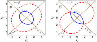
Figure 1: Fermi contours along with the two mirror symmetric lines $k_{y}=\pm k_{x}$ of a 2DEG with $k$-linear Rashba-Dresselhaus spin-orbit couplings for (a) $\alpha\neq\beta$ and (b) $\alpha=\beta$. Here, $k_{x}$ and $k_{y}$ are plotted in units of $k_{0}$.

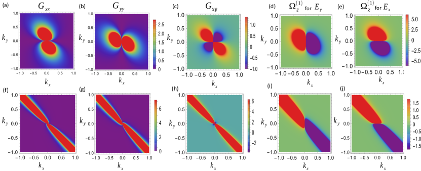
Figure 2: We present density plots of the band geometric quantities and the field-induced Berry curvature of the 2DEG with linear Rashba-Dresselhaus spin-orbit interactions: (top panel) $\alpha=6\times 10^{-9}$ eV cm and $\beta=1\times 10^{-9}$ eV cm and (bottom panel) $\alpha=6\times 10^{-9}$ eV cm and $\beta=5\times 10^{-9}$ eV cm. Here, (a)-(c) and (f)-(h) display the density plots of the BCP tensor components (in units of $e/\alpha{k_{0}^{3}}$), (d)-(e) and (i)-(j) display the field-induced Berry curvature $\Omega_{z}^{(1)}$ (in units of ${eE/\alpha k_{0}^{4}}$) for two orientations of the electric field along the $y$ and $x$ directions, respectively. The plots are given for the upper (+) band. We consider $m_{e}=0.024m_{0}$, where $m_{0}$ is the free electron masschang . In both the panels, $k_{x}$ and $k_{y}$ are in units of $k_{0}$.

The third-order current can be expressed in terms of third-order conductivity $\chi$ as $j^{(3)}_{a}=\chi_{abcd}E_{b}E_{c}E_{d}$, where the subscripts ${a,b,c,d}\in\{x,y\}$ and $\chi_{abcd}$ is a rank-4 tensor. The third-order conductivity tensor comprises two contributions, given by $\chi_{abcd}=\chi_{abcd}^{\text{I}}+\chi_{abcd}^{\text{II}}$, where $\chi_{abcd}^{\text{I}}$ is linear in $\tau$, and $\chi_{abcd}^{\text{II}}$ is proportional to $\tau^{3}$. These components can be derived as

$$\chi_{abcd}^{\text{I}} =\frac{-q^{3}\tau}{\hbar^{2}}\sum_{\lambda}\int[d\mathbf{k}]\Big{\{}\partial_{a}\partial_{b}G_{cd}^{\lambda}+\partial_{a}\partial_{d}G_{bc}^{\lambda}-\partial_{b}\partial_{d}G_{ac}^{\lambda}\Big{\}}f_{\text{eq}}^{\lambda}$$ (14)

$$+\frac{q^{3}\tau}{2}\sum_{\lambda}\int[d\mathbf{k}]v_{a,\lambda}v_{b,\lambda}G_{cd}^{\lambda}f_{\text{eq}}^{\prime\prime\lambda}$$

and

$$\chi_{abcd}^{\text{II}} =-\frac{q^{4}\tau^{3}}{\hbar^{3}}\sum_{\lambda}\int[d\mathbf{k}]v_{a,\lambda}\partial_{b}\partial_{c}\partial_{d}f_{\text{eq}}^{\lambda}.$$ (15)

Here, $\hbar\mathbf{v}_{\mathbf{k},\lambda}={\boldsymbol{\nabla}}_{\mathbf{k}}\epsilon_{\lambda}$ is the unperturbed band velocity. It is evident from Eqs. (14) and (15) that $\chi_{abcd}^{\text{I}}$ is associated with BCP, and $\chi_{abcd}^{\text{II}}$ is connected to the band dispersion. Next, we consider an in-plane electric field $\mathbf{E}=(E\cos\theta,E\sin\theta,0)$ such that the applied electric field forms an angle $\theta$ with respect to the $x$ axis. The third-order current within the plane can be described as

$$\left(\begin{matrix}{{j}^{(3)}_{x}}\\ \\ {{j}^{(3)}_{y}}\end{matrix}\right)=\left(\begin{matrix}{{\chi_{11}}{E_{x}^{3}}+3\chi_{12}{E_{x}}{E_{y}^{2}}+3\chi_{13}{E_{x}^{2}}{E_{y}}+\chi_{14}{E_{y}^{3}}}\\ \\ {\chi_{41}{E_{x}^{3}}+3\chi_{31}{E_{x}}{E_{y}^{2}}+3\chi_{21}{E_{x}^{2}}{E_{y}}+{\chi_{22}}{E_{y}^{3}}}\end{matrix}\right),$$ (16)

where we define $\chi_{11}=\chi_{xxxx}$, $\chi_{12}=(\chi_{xyyx}+\chi_{xyxy}+\chi_{xxyy})/3$, $\chi_{13}=(\chi_{xxxy}+\chi_{xyxx}+\chi_{xxyx})/3$, $\chi_{14}=\chi_{xyyy}$, $\chi_{41}=\chi_{yxxx}$, $\chi_{31}=(\chi_{yyyx}+\chi_{yxyy}+\chi_{yyxy})/3$, $\chi_{21}=(\chi_{yxxy}+\chi_{yxyx}+\chi_{yyxx})/3$ and $\chi_{22}=\chi_{yyyy}$. In nonlinear transport experiments, one measures the current response that is transverse to the electric field. Therefore, our focus lies in the third-order transverse current, which can be written as $j^{(3)}_{\perp}(\theta)=\mathbf{j}^{(3)}\cdot(\hat{\mathbf{z}}\times\hat{\mathbf{E}})$ and the associated third-order transverse conductivity is defined as $\chi_{\perp}(\theta)=j^{(3)}_{\perp}/E^{3}$. For a 2D system, the explicit form of $\chi_{\perp}(\theta)$ is given by

$$\chi_{\perp}(\theta)=(3\chi_{21}-\chi_{11})\cos^{3}\theta\sin\theta+(\chi_{22}-3\chi_{12})\sin^{3}\theta\cos\theta+3(\chi_{31}-\chi_{13})\cos^{2}\theta\sin^{2}\theta+\chi_{41}\cos^{4}\theta-\chi_{14}\sin^{4}\theta.$$ (17)

Importantly, the transverse third-order conductivities $\chi_{\perp}^{\text{I}}$ and $\chi_{\perp}^{\text{II}}$, proportional to $\tau$ and $\tau^{3}$, adopts the same form as that of $\chi_{\perp}$. This modification involves substituting $\chi_{abcd}$ by $\chi_{abcd}^{\text{I}}$ for $\chi_{\perp}^{\text{I}}$, and with $\chi_{abcd}^{\text{II}}$ for $\chi_{\perp}^{\text{II}}$. In the next section, we will apply this formalism to the Rashba-Dresselhaus system and investigate its third-order transverse conductivity.

III Two-dimensional electron gas with $k$-linear Rashba-Dresselhaus spin-orbit coupling

The Hamiltonian for a 2DEG with $k$-linear RSOI and DSOI is given byjohn ; shen

$$H=\frac{\hbar^{2}k^{2}}{2m_{e}}+\alpha(\sigma_{x}k_{y}-\sigma_{y}k_{x})+\beta(\sigma_{x}k_{x}-\sigma_{y}k_{y}).$$ (18)

Here, $\alpha$ and $\beta$ represent the strengths of RSOI and DSOI, $m_{e}$ denotes the effective mass of an electron and the $\sigma$’s are the Pauli matrices. The energy spectrum consists of two bands ($\lambda=\pm$) of the following form

$$\epsilon_{\lambda}(\mathbf{k})=\frac{\hbar^{2}k^{2}}{2m_{e}}+\lambda\sqrt{{(\alpha k_{y}+\beta k_{x})}^{2}+{(\alpha k_{x}+\beta k_{y})}^{2}}.$$ (19)

The corresponding eigenspinors can be obtained as $|{u}_{\lambda}\rangle=(1/\sqrt{2})[1\hskip 7.11317pt\lambda i\mathrm{e}^{i\varphi}]^{T}$, where $\varphi=\tan^{-1}[({\alpha k_{y}+\beta k_{x}})/({\alpha k_{x}+\beta k_{y}})]$ with $k_{x}=k\cos\phi$ and $k_{y}=k\sin\phi$ and $T$ being the transpose operation.

The two bands $\epsilon_{\lambda}(\mathbf{k})$ meet at ${\mathbf{k}}=0$, commonly called a band touching point (BTP). The energy difference between the two bands is given by $\epsilon_{g}(\mathbf{k})=2\Lambda_{\mathbf{k}}$ with $\Lambda_{\mathbf{k}}\equiv\Lambda=\sqrt{{(\alpha k_{y}+\beta k_{x})}^{2}+{(\alpha k_{x}+\beta k_{y})}^{2}}$. The maximum value of $\epsilon_{g}(\mathbf{k})$ at $\phi=\pi/4$ and $5\pi/4$ is $2k(\alpha+\beta)$, while the minimum value of $\epsilon_{g}(\mathbf{k})$ at $\phi=3\pi/4$ and $7\pi/4$ is $2k|\alpha-\beta|$. These values of $\phi$ also coincide with the symmetry lines $k_{x}\pm k_{y}=0$ of the system. There is a line degeneracy along the symmetry line $k_{y}+k_{x}=0$ for $\alpha=\beta$ case as shown Fig. 1.

The wave vectors corresponding to $\epsilon>0$ are given by $\tilde{k}_{\lambda}(\phi)=-\lambda\sqrt{\gamma}+\sqrt{2\tilde{\epsilon}+\gamma}$, where we define $\gamma=1+\zeta^{2}+2\zeta\sin 2\phi$, with $\zeta=\beta/\alpha$. We introduce the scaled parameters $\tilde{k}=k/k_{0}$ and $\tilde{\epsilon}=\epsilon/\epsilon_{0}$ with $k_{0}=m\alpha/\hbar^{2}$ and $\epsilon_{0}=m\alpha^{2}/\hbar^{2}$ as scaled wave vector and energy, respectively. For $\epsilon<0$, only one energy band with $\lambda=-$ contributes and it attains a minimum value of $\tilde{\epsilon}_{\text{min}}=-\gamma/2$. The associated wave vectors can be expressed as $\tilde{k}_{\eta}(\phi)=\sqrt{\gamma}-{(-1)}^{\eta-1}\sqrt{2\tilde{\epsilon}+\gamma}$, where $\eta=1,2$ is the branch index.

We consider the following key points in order to study the TOH response of this system. The conventional Berry curvature of the system vanishes everywhere except for a singular nature at the degenerate point $\mathbf{k}=0$. As a result, the linear anomalous Hall effect and Berry curvature dipole induced second-order Hall response vanish. Hence, the BCP induced third-order Hall response will be the dominant one in the $k$-linear Rashba-Dresselhaus system. To determine the third-order conductivity, one can compute the different components of the BCP tensor using Eq. (7) as

$$G_{ab}^{\lambda}=\lambda\frac{e{(\alpha^{2}-\beta^{2})}^{2}}{4\Lambda^{5}}\left(\begin{matrix}{k_{y}^{2}}&{-k_{x}k_{y}}\\ {-k_{x}k_{y}}&{k_{x}^{2}}\end{matrix}\right),$$ (20)

We have plotted the density plots of these BCP tensor elements $G_{xx}$, $G_{yy}$ and $G_{xy}$ for $\beta\ll\alpha$ in Figs. 2(a)-2(c), respectively. The diagonal elements $G_{xx}$ and $G_{yy}$ exhibit a dumbbell-like pattern, whereas the off-diagonal element $G_{xy}$ shows a quadrupole-like structure. Under an in-plane electric field, the field-induced Berry curvature can be written in terms of BCP tensor asliu $\boldsymbol{\Omega}^{(1)}_{\lambda}=[({\partial_{k_{x}}}G_{yx}^{\lambda}-{\partial_{k_{y}}}G_{xx}^{\lambda})E_{x}+({\partial_{k_{x}}}G_{yy}^{\lambda}-{\partial_{k_{y}}}G_{xy}^{\lambda})E_{y}]\hat{\mathbf{z}}.$ We find that for this system, the second-order energy correction and field-induced Berry curvature can be obtained as

$$\epsilon_{\lambda}^{(2)}=\lambda\frac{e^{2}{(\alpha^{2}-\beta^{2})}^{2}}{8\Lambda^{5}}(\mathbf{E}\times\mathbf{k})^{2}$$ (21)

and

$$\boldsymbol{\Omega}^{(1)}_{\lambda}(\mathbf{k})=\lambda\frac{e{(\alpha^{2}-\beta^{2})}^{2}}{2\Lambda^{5}}(\mathbf{E}\times\mathbf{k}).$$ (22)

It should be mentioned here that expressions of $\epsilon_{\lambda}^{(2)}$ and $\boldsymbol{\Omega}^{(1)}_{\lambda}(\mathbf{k})$ are obtained using the non-degenerate perturbation theory. Therefore Eqs. (21) and (22) are not valid at $\alpha=\beta$ case, since there is a line degeneracy along the symmetry line $k_{y}+k_{x}=0$ for $\alpha=\beta$ case.

Unlike the Berry curvature, the field-induced Berry curvature remains finite and exhibits a dipole-like structure. It is directed out-of-plane, but its orientation is sensitive to the applied electric field. Figures 2(f)-2(j) further depict that as the values of $\alpha$ approach close to $\beta$, the lobes in the diagonal element of BCP and $\Omega_{z}^{(1)}$ undergo substantial elongation. In the case of $G_{xy}$, the lobes experience stretching in one direction, accompanied by a corresponding contraction in the orthogonal direction. Note that these BCP tensor elements and ${\Omega}_{z}^{(1)}$ are concentrated around the BTP. Figure 2 clearly demonstrates that the lobes in diagonal components of BCP and ${\Omega}_{z}^{(1)}$ are confined in the $x$-$y$ plane. This observation can be understood from the system’s anisotropic nature resulting from $\alpha\neq\beta$. For the pure Rashba system ($\beta=0$), the lobes are exclusively aligned along the $x$ and $y$ directions.

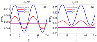
Figure 3: Polarization (in units of $P_{0}=e^{2}E/\epsilon_{0}$) as a function of angle $\theta$ for different Dresselhaus coupling strengths (in units of $10^{-9}$ eV cm) at a fixed Rashba coupling strength of $\alpha=6\times 10^{-9}$ eV cm: (a) $\epsilon_{F}>0$ at a fixed electron density of $n_{e}=5.7\times 10^{10}$/cm² and (b) $\epsilon_{F}<0$ at $n_{e}=10^{10}$/cm². The other parameters used are the same as in Fig. 2.

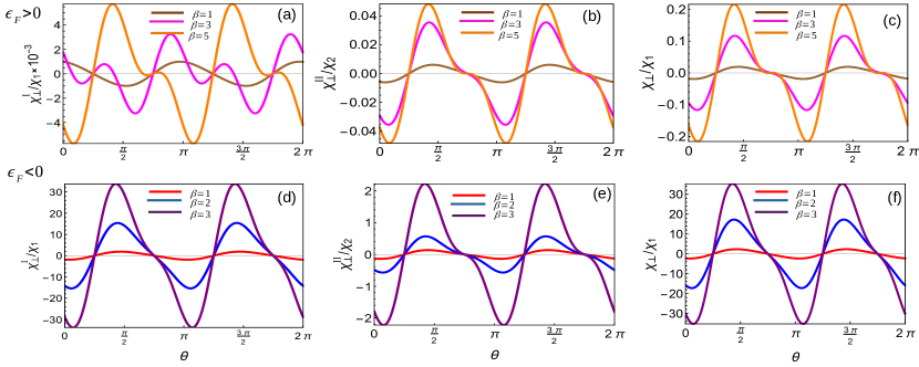
Figure 4: Variation of the transverse third-order conductivities with angle $\theta$ for different Dresselhaus coupling strengths, while keeping the Rashba coupling strength fixed at $\alpha=6\times 10^{-9}$ eV cm. The conductivities $\chi_{\perp}^{\text{I}}$ and $\chi_{\perp}^{\text{II}}$ correspond to transverse third-order conductivities proportional to $\tau$ and $\tau^{3}$, respectively. The total transverse conductivity is given by $\chi_{\perp}=\chi_{\perp}^{\text{I}}+\chi_{\perp}^{\text{II}}$. The top panel (a)-(c) represents the case for $\epsilon_{F}>0$, and the bottom panel (d)-(f) corresponds to the scenario where $\epsilon_{F}<0$. The normalization parameters for conductivities, $\chi_{\perp}^{\text{I}}$ and $\chi_{\perp}^{\text{II}}$, are given by $\chi_{1}={\tau e^{4}\hbar^{4}}/{m_{e}^{3}\alpha^{4}}$ and $\chi_{2}={e^{4}\tau^{3}}/{m_{e}\hbar^{2}}$, respectively. The value of $\beta$ is given in units of $10^{-9}$ eV cm. The $\beta=5$ curve is scaled by factors of 50 in (a) and 5 in (b) and (c), while the $\beta=3$ curve is scaled down by factors of 5 in (d) and (f). The parameters used are same as in Fig. 3.

III.1 Polarization

For the pure Rashba system ($\beta=0$), an analytical expression of the electric polarization can be obtained using Eq. (10) as

$$P=\frac{P_{0}}{16\pi}\begin{cases}\frac{1}{N_{e}-1},&N_{e}>1,\\ \frac{2N_{e}}{1-N_{e}^{2}},&N_{e}<1,\end{cases}$$ (23)

where $P_{0}=e^{2}E/\epsilon_{0}$ and $N_{e}=\pi l_{e}^{2}n_{e}$ with $l_{e}=\hbar^{2}/(m_{e}\alpha)$. Note that the Fermi energy is zero at the BTP which can be reached if $N_{e}=\pi l_{e}^{2}n_{e}=1$. For $\alpha=0$ but $\beta\neq 0$, the polarization can be obtained from Eq. (23) with $\alpha$ replaced by $\beta$. We find that the polarization decreases with the increase in Fermi energy, reflecting the behavior of the BCP. It is important to note that the polarization does not vary with the angle $\theta$ (between the electric field and $x$ axis) since contribution from $G_{xy}\propto k_{x}k_{y}$ vanishes upon angular integration, as $\int_{0}^{2\pi}\sin 2\phi d\phi=0$. Both $G_{xx}$ and $G_{yy}$ contributes equally, rendering it insensitive to orientation of the electric field in the case of $\beta=0$.

We have also illustrated the dependence of polarization on $\theta$ under the influence of both the couplings in Figs. 3(a) and 3(b) for ${\epsilon}_{F}>0$ and ${\epsilon}_{F}<0$, respectively. This demonstrates that adding an infinitesimal DSOI to the RSOI makes polarization responsive to the electric field orientation, as $G_{xy}$ also contributes. Therefore, the polarization takes the following form: $P=-eE\sum_{\lambda}\int[d\mathbf{k}](G_{xx}^{\lambda}+G_{xy}^{\lambda}\sin 2\theta)$. The integration of $G_{xx}$ and $G_{xy}$ yields the positive values for the given set of parameters. Consequently, the polarization is maximum at $\theta=\pi/4$ and $5\pi/4$ and minimum at $\theta=3\pi/4$ and $7\pi/4$. These values of $\theta$ coincides with the symmetry lines of the system. The magnitude of polarization increases with an increase in $\beta$ for a given $\alpha$. The electric polarization in ${\epsilon}_{F}<0$ region is large as compared to ${\epsilon}_{F}>0$. This is due to the Van Hove singularity in the density of states as Fermi energy approaches the band minimum, $\epsilon_{F}\rightarrow\epsilon_{\text{min}}$.

III.2 Third-order transverse conductivity

In the Rashba-Dresselhaus system, where both $\alpha$ and $\beta$ are nonzero, the lines $k_{x}=\pm k_{y}$ serve as symmetry axes of the system. Due to the underlying symmetry axes of the system, we have $\chi_{11}=\chi_{22}$, $\chi_{12}=\chi_{21}$, $\chi_{31}=\chi_{13}$, and $\chi_{14}=\chi_{41}$, which reduces Eq. (17) to

$$\chi_{\perp}(\theta)=\frac{1}{4}(3\chi_{21}-\chi_{11})\sin 4\theta+\chi_{41}\cos{2}\theta.$$ (24)

The vanishing behavior of $\chi_{\perp}$ along or perpendicular to the symmetry lines of the system can be understood well from the above equation. Both the terms $\sin 4\theta$ and $\cos 2\theta$ of Eq. (24) vanish simulatneously whenever $\theta\in\left\{{\pi}/{4},{3\pi}/{4},{5\pi}/{4},{7\pi}/{4}\right\}$, independent of the system parameters. These four angles coincide with the symmetry lines of the systems. If we consider $\theta=0$, then $\chi_{\perp}=\chi_{41}=\chi_{yxxx}$. Below, we will discuss the contributions to transverse conductivity based on their scaling relation with $\tau$.

$\tau$- scaling conductivity ($\chi_{\perp}^{\text{I}}$): We numerically evaluate $\chi_{\perp}^{\text{I}}$ for the system, considering both $\epsilon_{F}>0$ and $\epsilon_{F}<0$. For the isotropic Rashba system ($\beta=0$), we observe that $\chi_{11}=3\chi_{21}$ and $\chi_{41}=0$. Consequently, $\chi_{\perp}^{\text{I}}$ vanishes for all Fermi energies. For Fermi energies above the BTP, we perform the calculations at a constant electron density of $n_{e}=5.7\times 10^{10}$/cm² and a fixed Rashba coupling strength of $\alpha=6\times 10^{-9}$ eV cm, while systematically varying the Dresselhaus coupling parameter $\beta$. The variation of $\chi_{\perp}^{\text{I}}$ as a function of the angle $\theta$ for different values of $\beta$ is shown in Fig. 4(a). We find that when the value of $\beta$ is much smaller than $\alpha$, let’s say $\beta=1$, we obtain a finite $\chi_{\perp}^{\text{I}}$ that exhibits significant dependence on the $\cos 4\theta$ term. The system exhibits more anisotropic behavior as we further increase $\beta$, a competition arises between the coefficients of $\sin 4\theta$ and $\cos 2\theta$, which is clearly illustrated in Fig. 4(a). We also observe the presence of additional angles $\theta$ at which $\chi_{\perp}^{\text{I}}$ vanishes. Note that these angles of additional zeros depend on the system parameters. They manifest symmetrically around the zeros that originate from the inherent symmetry of the system, i.e., $\theta=\pi/4,3\pi/4,5\pi/4,7\pi/4$. Additionally, it can be noted that the magnitude of $\chi_{\perp}^{\text{I}}$ increases significantly as $\beta$ approaches close to $\alpha$ (as shown here for $\beta=5$). At $\alpha=\beta$, $\chi_{\perp}^{\text{I}}=0$. This behavior can be attributed to the characteristics of the BCP tensor. The variation of $\chi_{\perp}^{\text{I}}$ with $\theta$ exhibits a periodicity of $\pi$. On the other hand, the magnitude of $\chi_{\perp}^{\text{I}}$ for $\epsilon_{F}<0$ (${\epsilon}_{\text{min}}<\epsilon_{F}<0$) is notably larger compared to $\epsilon_{F}>0$, as depicted in Fig. 4(d). At Fermi energies below the BTP, the conductivity increases significantly as the Fermi energy approaches the band minimum, attributed to the Van Hove singularity in the density of states as $\epsilon_{F}\rightarrow\epsilon_{\text{min}}$.

One can determine the maxima and minima of $\chi_{\perp}$ by differentiating Eq. (24) with respect to $\theta$ and set it zero. Then we obtain locations of maxima and mimima for various system parameters. The values of the coefficients of $\sin 4\theta$ and $\cos 2\theta$ of Eq. (24) change with $\alpha$ and $\beta$, leading to shifts in the positions of maxima and minima and emphasizing their dependence on system parameters.

It is important to emphasize that the magnitude and sign of $\chi_{\perp}^{\text{I}}$ remain unaltered when the values of $\alpha$ and $\beta$ are interchanged. For instance, $\chi_{\perp}^{\text{I}}(\alpha=2,\beta=6$) = $\chi_{\perp}^{\text{I}}(\alpha=6,\beta=2$). This finding can be explained by the invariance of the Hamiltonian under $\alpha\leftrightarrow\beta$ and rotation by the unitary rotation operator, $U=e^{-i\frac{\pi}{4}\sigma_{z}}e^{-i\frac{\pi}{2}\sigma_{y}}$, which transforms $\sigma_{x}\rightarrow-\sigma_{y}$, $\sigma_{y}\rightarrow-\sigma_{x}$, and $\sigma_{z}\rightarrow-\sigma_{z}$. Both the unperturbed velocity operator and the velocity resulting from the second-order energy correction, which is related to the BCP tensor, also remain invariant under these transformations. Thus the third-order current is same when $\alpha$ and $\beta$ are exchanged.

We also explore the dependence of third-order conductivity on the Fermi energy. Keeping the electron density and Rashba coupling $\alpha$ fixed, an increase in $\beta$ leads to a reduction in the Fermi energy. Consequently, we find that the magnitude of $\chi_{\perp}^{\text{I}}$ increases as the Fermi energy decreases. This understanding can be derived from the behavior of the BCP tensors, which exhibit a maximal value at the degenerate point and gradually decrease as one moves away from it.

$\tau^{3}$-scaling conductivity ($\chi_{\perp}^{\text{II}}$): We also evaluate the transverse third-order conductivity $\chi_{\perp}^{\text{II}}$, which is proportional to $\tau^{3}$ and solely arises from the band velocity. We find that $\chi_{\perp}^{\text{II}}$ also vanishes for a pure Rashba system, as $\chi_{11}=3\chi_{21}$ and $\chi_{41}=0$. The dependence of $\chi_{\perp}^{\text{II}}$ on $\theta$ for different coupling strengths is illustrated in Figs. 4(b) and 4(e), corresponding to $\epsilon_{F}>0$ and $\epsilon_{F}<0$, respectively. For $\epsilon_{F}>0$, using the same parameters as those employed for $\chi_{\perp}^{\text{I}}$, we note that with increasing $\beta$, the magnitude of $\chi_{\perp}^{\text{II}}$ increases and exhibits a more pronounced anisotropic growth. We highlight two distinct behaviors of $\chi_{\perp}^{\text{II}}$: (i) there are no additional zeroes observed for any values of $\beta$, and (ii) in contrast to the case of $\chi_{\perp}^{\text{I}}$, the magnitude of $\chi_{\perp}^{\text{II}}$ does not show a drastic increase as $\beta$ approaches $\alpha$. This occurs because the BCP increases more rapidly as $\beta$ approaches $\alpha$, compared to the band velocity, which straightforwardly affects their respective contributions to the conductivity. The magnitude of $\chi_{\perp}^{\text{II}}$ is greater for $\epsilon_{F}<0$ when compared to the case of $\epsilon_{F}>0$. The magnitude and sign of $\chi_{\perp}^{\text{II}}$ also remain unchanged upon the interchange of $\alpha$ and $\beta$, along with a similar unitary transformation.

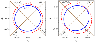
Figure 5: Fermi contours along with the two mirror symmetric lines $k_{y}=\pm k_{x}$ of the 2DHG with $k$-cubic Rashba-Dresselhaus spin-orbit couplings for (a) $\alpha_{h}\neq\beta_{h}$ and (b) $\alpha_{h}=\beta_{h}$. Here, $k_{x}$ and $k_{y}$ are plotted in units of $k_{h}$.

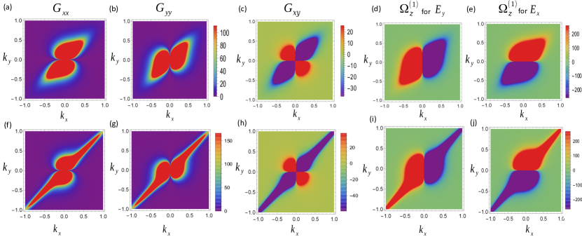
Figure 6: Distribution of the BCP tensors and the field-induced Berry curvature for + branch of a 2DHG with $k$-cubic Rashba-Dresselhaus spin-orbit interactions: (top panel) ${\alpha_{h}}=0.1$ eV nm³ and ${\beta_{h}}=0.6{\alpha_{h}}$, and (bottom panel) ${\alpha_{h}}=0.1$ eV nm³ and ${\beta_{h}}=0.9{\alpha_{h}}$. Here, (a)-(c) and (f)-(h) represent the density plots of the BCP tensor components (in units of $-e/\alpha_{h}{k_{h}^{5}}$), (d)-(e) and (i)-(j) represent the field-induced Berry curvature $\Omega_{z}^{(1)}$ (in units of ${-eE/\alpha_{h}k_{h}^{6}}$) for two orientations of the electric field along the $y$ and $x$ directions, respectively. In both panels, $k_{x}$ and $k_{y}$ are plotted in units of $k_{h}$. We consider $m_{h}=0.41m_{0}$, where $m_{0}$ is the free electron mass.

Net transverse conductivity ($\chi_{\perp}$): We also explore the third-order transverse conductivity, which comprises two components proportional to $\tau$ and $\tau^{3}$, denoted as $\chi_{\perp}=\chi_{\perp}^{\text{I}}+\chi_{\perp}^{\text{II}}$. Extracting these two conductivities individually in an experimental setting proves challenging. Therefore, providing their combined contributions becomes a valuable approach at very low temperatures. However, the separation of these contributions has been demonstrated through temperature scaling analysiscwang . We present the variation of $\chi_{\perp}/\chi_{1}$ as a function of $\theta$ for both $\epsilon_{F}>0$ and $\epsilon_{F}<0$ in Figs. 4(c) and (f). We have $\chi_{\perp}/\chi_{1}=\chi_{\perp}^{\text{I}}/\chi_{1}+(\chi_{\perp}^{\text{II}}/\chi_{2})(\chi_{2}/\chi_{1})$ with $\chi_{2}/\chi_{1}=3.29$ for $\tau=1$ ps. When $\beta$ is significantly smaller than $\alpha$, the magnitude of $\chi_{\perp}^{\text{II}}$ surpasses that of $\chi_{\perp}^{\text{I}}$, resulting in the behavior of $\chi_{\perp}$ resembling that of $\chi_{\perp}^{\text{II}}$. When $\beta$ approaches values close to $\alpha$, both $\chi_{\perp}^{\text{I}}$ and $\chi_{\perp}^{\text{II}}$ become comparable. Consequently, we also observe additional zeros in the behavior of $\chi_{\perp}$, mirroring the pattern seen in $\chi_{\perp}^{\text{I}}$ for $\beta=5$.

Based on our calculations, we provide an estimate of the third-order Hall current that can potentially manifest during experimental observations. The third-order Hall current can be defined as $I=j^{(3)}_{\perp}l_{0}$, where $j^{(3)}_{\perp}=\chi_{\perp}E^{3}$ and $l_{0}$ represents the length of the sample. For an uniform electric field of $100$ V/cm, $l_{0}=1$ mm, $\tau=1$ ps, $\theta=\pi/2$, and utilizing system parameters such as $\alpha=6\times 10^{-9}$ eV cm, $\beta=1\times 10^{-9}$ eV cm and $\epsilon_{F}=4.27$ meV, the third-order Hall current can be calculated as $I\sim 15$ ${\mu}$A.

IV Two-dimensional hole gas with $k$-cubic Rashba-Dresselhaus spin-orbit coupling

The effective Hamiltonian of a heavy-hole gas with $k$-cubic RSOI and DSOI formed at the p-type III-V semiconductor heterostructures is given byloss ; john1 ; mireles

$$H =\frac{\hbar^{2}k^{2}}{2m_{h}}+{i\alpha_{h}}\Big{(}k_{-}^{3}\sigma_{+}-k_{+}^{3}\sigma_{-}\Big{)}$$ (25)

$$-{\beta_{h}}\Big{(}k_{-}k_{+}k_{-}\sigma_{+}+k_{+}k_{-}k_{+}\sigma_{-}\Big{)},$$

where $k_{\pm}=k_{x}\pm ik_{y}$, $\sigma_{\pm}=(\sigma_{x}\pm i\sigma_{y})/2$, with $\sigma_{i}$’s as the Pauli spin matrices and $m_{h}$ is the effective heavy-hole mass. Also, $\alpha_{h}$ and $\beta_{h}$ are the strength of RSOI and DSOI, respectively. The energy spectrum is given by

$$\epsilon_{\lambda}\mathbf{(k)}=\frac{\hbar^{2}k^{2}}{2m_{h}}+\lambda k^{2}\sqrt{{(\alpha_{h}k_{x}-\beta_{h}k_{y})}^{2}+{(\alpha_{h}k_{y}-\beta_{h}k_{x})}^{2}},$$ (26)

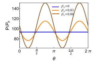
Figure 7: Polarization (in units of $P_{h}=e^{2}E/\epsilon_{h}$) for a hole gas with angle $\theta$ for different Dresselhaus coupling strengths (given in units of eV nm³) at a fixed Rashba coupling strength $\alpha_{h}=0.1$ eV nm³. The other parameters used are charge carrier density $n_{h}=2\times 10^{15}$ m^-2 and ${m_{h}}=0.41{m_{0}}$alestin .

where $\lambda=\pm$ denotes the two dispersive branches. The corresponding eigenspinors can be calculated as $|{u}_{\lambda}\rangle=(1/\sqrt{2})[1\hskip 7.11317pt\lambda\mathrm{e}^{i(2\phi-\phi^{\prime})}]^{T}$, where $\phi^{\prime}=\tan^{-1}[({\alpha_{h}k_{x}-\beta_{h}k_{y}})/({\alpha_{h}k_{y}-\beta_{h}k_{x}})]$ with $k_{x}=k\cos\phi$ and $k_{y}=k\sin\phi$. The spin splitting energy between the two branches, $\epsilon_{g}(\mathbf{k})=\epsilon_{+}(\mathbf{k})-\epsilon_{-}(\mathbf{k})=2k^{2}\Delta_{\mathbf{k}}$, with $\Delta_{\mathbf{k}}\equiv\Delta=\sqrt{(\alpha_{h}k_{x}-\beta_{h}k_{y})^{2}+(\alpha_{h}k_{y}-\beta_{h}k_{x})^{2}}$. In polar form, it can be expressed as $\epsilon_{g}(\mathbf{k})=2k^{3}\vartheta(\phi)$, where $\vartheta(\phi)\equiv\vartheta=\sqrt{\alpha_{h}^{2}+\beta_{h}^{2}-2\alpha_{h}\beta_{h}\sin 2\phi}$. It is to be noted that the lower branch of the Hamiltonian is valid for the wave numbers $k\leq\hbar^{2}/(2m_{h}\vartheta)$. The maximum value of $\epsilon_{g}(\mathbf{k})$ at $\phi=3\pi/4$ and $7\pi/4$ is $2k^{3}(\alpha_{h}+\beta_{h})$, and the minimum value of $\epsilon_{g}(\mathbf{k})$ at $\phi=\pi/4$ and $5\pi/4$ is $2k^{3}|\alpha_{h}-\beta_{h}|$. These values of $\phi$ also coincide with the symmetry lines $k_{x}\pm k_{y}=0$ of the system. There is a line degeneracy along the symmetry line $k_{y}-k_{x}=0$ for $\alpha_{h}=\beta_{h}$ case as shown in Fig. 5.

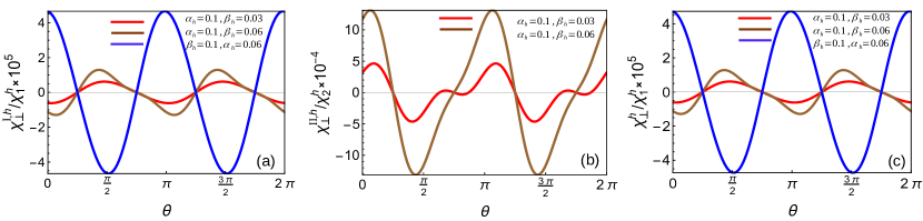
Figure 8: (a)-(c) Variation of the transverse third-order conductivities for the heavy-hole gas with $k$-cubic Rashba-Dresselhaus spin-orbit interactions as a function of the angle $\theta$ between the electric field and the $x$-axis. The conductivities $\chi_{\perp}^{\text{I},h}$ and $\chi_{\perp}^{\text{II},h}$ represent the transverse third-order conductivities of the hole gas proportional to $\tau$ and $\tau^{3}$, respectively. The total transverse conductivity is given by $\chi_{\perp}^{h}=\chi_{\perp}^{\text{I},h}+\chi_{\perp}^{\text{II},h}$. In (b), $\chi_{\perp}^{\text{II},h}$ ($\alpha_{h}=0.1$ and $\beta_{h}=0.06$) = $\chi_{\perp}^{\text{II},h}$ ($\beta_{h}=0.1$ and $\alpha_{h}=0.06$). The normalization parameters for conductivities, $\chi_{\perp}^{\text{I},h}$ and $\chi_{\perp}^{\text{II},h}$, are given by $\chi_{1}^{h}={\tau e^{4}m_{h}^{5}\alpha^{4}}/{\hbar^{12}}$ and $\chi_{2}^{h}={e^{4}\tau^{3}}/{m_{h}\hbar^{2}}$, respectively. The value of $\alpha_{h}$ and $\beta_{h}$ are given in units of eV nm³. The parameters used are the same as in Fig. 7.

The analytical derivation of wave vectors is not feasible for the anisotropic hole system. Hence, we numerically evaluate the wave vectors by solving the cubic equation, $\hbar^{2}k^{2}/2m_{h}+\lambda k^{3}\vartheta-\epsilon=0$. However, when $\beta_{h}$ is set to zero, exact expressions for the Fermi wave vectors can be obtained analyticallyjohn1 . The scaled wave vector and energy are defined as $\tilde{k}_{h}=k/k_{h}$ and $\tilde{\epsilon}=\epsilon/\epsilon_{h}$, where $k_{h}=\hbar^{2}/({m_{h}\alpha_{h}})$ and $\epsilon_{h}=\alpha_{h}{k_{h}^{3}}$.

The Berry connection for the system can be calculated as $\mathbf{A}_{\mathbf{k}}=\frac{\delta}{2k^{2}{\Delta}^{2}}(k_{y}\hat{x}-k_{x}\hat{y})$, where $\delta=[(3\alpha_{h}^{2}+\beta_{h}^{2})(k_{x}^{2}+k_{y}^{2})-8\alpha_{h}\beta_{h}k_{x}k_{y}]$. The Berry curvature is zero, which leads to the absence of linear and second-order Hall responses, making the third-order Hall response dominant for the hole system as well. To calculate the third-order conductivity, one can evaluate the different components of the BCP tensor for the system as

$$G_{ab}^{\lambda}=-\lambda\frac{e\delta^{2}}{4\Delta^{5}{k}^{6}}\left(\begin{matrix}{k_{y}^{2}}&{-k_{x}k_{y}}\\ {-k_{x}k_{y}}&{k_{x}^{2}}\end{matrix}\right).$$ (27)

Similar to the electron case, Eq. (27) is not valid for $\alpha_{h}=\beta_{h}$ because of the presence of the line degeneracy along symmetry line $k_{y}-k_{x}=0$. The distribution of the BCP tensor components in the $k_{x}$-$k_{y}$ plane for $\alpha_{h}=0.1$ eV nm³ and $\beta_{h}=0.6\alpha_{h}$ is plotted in Figs. 6(a)-6(c). The diagonal components $G_{xx}$ and $G_{yy}$ show a dumbbell-like structure, whereas $G_{xy}$ exhibits quadrupole-like features. On applying an in-plane electric field, the second-order energy correction and the field-induced Berry curvature can be obtained as

$$\epsilon_{\lambda}^{(2)}=\lambda\frac{e^{2}{\delta^{2}}}{8k^{6}\Delta^{5}}(\mathbf{E}\times\mathbf{k})^{2}\hskip 8.5359pt\text{and}\hskip 8.5359pt\boldsymbol{\Omega}^{(1)}_{\lambda}(\mathbf{k})=-\lambda\frac{e{\delta^{2}}}{k^{6}\Delta^{5}}(\mathbf{E}\times\mathbf{k}).$$ (28)

Similar to the electron gas case, we observe that $\Omega_{z}^{(1)}$ exhibits a dipole-like structure with its orientation changing relative to the electric field direction, as depicted in Figs. 6(d)-6(e). When $\beta_{h}$ is zero, the lobes align precisely along the $x$ and $y$ axes. As we increase $\beta_{h}$, anisotropy is introduced into the system, causing the lobes in the BCP components and $\Omega_{z}^{(1)}$ to align within the $x$-$y$ plane. Further increase of $\beta_{h}$ results in the stretching of lobes, as shown in Figs. 6(f)-6(j).

IV.1 Polarization

Similar to the electron case, we obtain an analytical expression for the electric polarization of 2DHG with $k$-cubic RSOI $(\beta_{h}=0)$,

$$P=\frac{3{P_{h}}}{2\pi}\Big{[}\frac{3(1+\sqrt{1-16\pi{n}_{h}l_{h}^{2}})-32\pi n_{h}l_{h}^{2}}{16\pi n_{h}l_{h}^{2}(1-16\pi n_{h}l_{h}^{2})^{3/2}}\Big{]},$$ (29)

where $P_{h}=e^{2}E/\epsilon_{h}$ and $l_{h}=m_{h}\alpha_{h}/\hbar^{2}$. For $\alpha_{h}=0$ and $\beta_{h}\neq 0$, the polarization is reduced by a factor of nine. Here as well, polarization remains constant with $\theta$ when either one of the spin-orbit couplings is absent, for similar reasons as specified in the electron case. The variation of polarization with $\theta$ in the presence of both the couplings is depicted in Fig. 7. The polarization increases with $\beta_{h}$, while decreases with the Fermi energy. When both $\alpha_{h}$ and $\beta_{h}$ are nonzero, the integration of $G_{xx}$ and $G_{xy}$ yield positive and negative values, respectively. Thus, the maximum of polarization is observed at $\theta=3\pi/4$ and $7\pi/4$ and minimum at $\theta=\pi/4$ and $5\pi/4$. This is in contrast to the electron case.

For a positive Fermi energy, the polarization of a $k$-linear electron gas with RSOI and DSOI is of an order of magnitude smaller than that for a hole gas with $k$-cubic couplings.

IV.2 Third-order transverse conductivity

The $k$-cubic Rashba-Dresselhaus system acquires the same form of $\chi_{\perp}$ as described in Eq. (24), owing to the same symmetry lines $k_{x}\pm k_{y}=0$. Next, we discuss the contribution of $\chi_{\perp}$ proportional to $\tau$ and $\tau^{3}$ given by Eqs. (14) and (15) for the hole system.

$\tau$-scaling conductivity ($\chi_{\perp}^{\text{I},h}$): We evaluate $\chi_{\perp}^{\text{I},h}$ numerically for different values of $\alpha_{h}$ and $\beta_{h}$, and its variation with respect to $\theta$ is depicted in Fig. 8(a). In our calculations, we consider the parameters representing p-type InAs heterostructuresalestin : hole density $n_{h}=2\times 10^{15}$ m^-2 and $m_{h}=0.41m_{0}$, and $\alpha_{h}=0.1$ eV nm³, while varying $\beta_{h}$. In an isotropic cubic Rashba system, $\chi_{\perp}^{\text{I},h}$ is zero since $3\chi_{21}=\chi_{11}$ and $\chi_{41}=0$. However, when a finite small value of $\beta_{h}$ is introduced, $\chi_{\perp}^{\text{I},h}$ becomes finite and exhibits a significant dependence on the $\cos 2\theta$ term. It is important to note that as we increase $\beta_{h}$ from 0.1$\alpha_{h}$ to 0.5$\alpha_{h}$, the curve of $\chi_{\perp}^{\text{I},h}$ follows qualitatively a similar pattern but with an increased magnitude. This happens because the BCP is proportional to $\delta^{2}$ and more specifically, the coefficient associated with $\alpha_{h}$ is three times that of $\beta_{h}$. Therefore, as $\beta_{h}$ is increased, the impact on $\delta^{2}$ is less pronounced compared to changes in $\alpha_{h}$, resulting in the observed pattern of $\chi_{\perp}^{\text{I},h}$ with a higher magnitude but similar overall shape. As $\beta_{h}$ is further increased, anisotropic curves emerge from the interplay between the coefficients of $\sin 4\theta$ and $\cos 2\theta$. Similar to the electron scenario, we notice additional angles at which $\chi_{\perp}^{\text{I},h}$ vanishes, beyond those dictated by the system’s inherent symmetry. Note that these angles of additional zeros depend on the system parameters. The positions of maxima and minima shift as one varies $\alpha_{h}$ and $\beta_{h}$, emphasizing their dependence on system parameters.

Upon applying a unitary transformation $U$ similar to that used for the electron case and interchanging the values of $\alpha_{h}$ and $\beta_{h}$, the transformed Hamiltonian no longer remains invariant. The perturbed velocity resulting from $\epsilon_{\lambda}^{(2)}$ changes under such transformations. Therefore, the third-order conductivity ($\propto\tau$) ceases to remain invariant under $\alpha_{h}\leftrightarrow\beta_{h}$, as evident in Fig. 8(a).

$\tau^{3}$-scaling conductivity ($\chi_{\perp}^{\text{II},h}$): The variation of $\chi_{\perp}^{\text{II},h}$ as a function of $\theta$ for the same set of parameters is shown in Fig. 8(b). We find that the $\chi_{\perp}^{\text{II},h}$ vanishes for an isotropic Rashba system ($\beta_{h}=0$), for the same underlying reason observed for $\chi_{\perp}^{\text{I},h}$. The magnitude of $\chi_{\perp}^{\text{II},h}$ increases with the $\beta_{h}$, while keeping $\alpha_{h}$ fixed. When $\alpha_{h}=\beta_{h}$, $\chi_{\perp}^{\text{II},h}$ becomes zero due to equal and opposite contributions from both the branches. The magnitude and sign of $\chi_{\perp}^{\text{II},h}$ remains unchanged upon interchanging $\alpha_{h}$ and $\beta_{h}$ is a direct consequence of its origin in the unperturbed velocity, which remains insensitive to such transformations.

Net transverse conductivity ($\chi_{\perp}^{h}$): In Fig. 8(c), we present the variation of the net contribution $\chi_{\perp}^{h}$ arising from $\tau$ and $\tau^{3}$. It is worth noting that the magnitude of $\chi_{\perp}^{\text{II},h}$ is smaller than that of $\chi_{\perp}^{\text{I},h}$ for a hole gas. As a result, the behavior of $\chi_{\perp}^{h}$ exhibits similarity to that of $\chi_{\perp}^{\text{I},h}$. Like $\chi_{\perp}^{\text{I},h}$ and $\chi_{\perp}^{\text{II},h}$, $\chi_{\perp}^{h}$ varies with $\theta$ with a period of $\pi$.

For the Hall setup with the same parameters as those employed for the electron case and the system parameters specified as $\alpha_{h}=0.1$ eV nm³ and $\beta_{h}=0.3\alpha_{h}$, the estimated third-order Hall current for the hole gas with $k$-cubic RSOI and DSOI is $I_{h}\sim 12$ ${\mu}$A.

V conclusion

In this study, we investigated the electric polarization and third-order Hall response in a 2D electron/hole gas with $k$-linear/$k$-cubic RSOI and DSOI present at III-V semiconductor heterostructures. We have obtained the analytical expressions of the BCP tensors and the field-induced Berry curvature. We have also obtained analytical expressions for the BCP-induced electric polarization when either Rashba or Dresselhaus spin-orbit interaction is present. The electric polarization decreases with an increase in the Fermi energy, while it increases with the Dresselhaus coupling for a given Rashba coupling. We find that the polarization is sensitive to the orientation of the electric field when both Rashba and Dresselhaus spin-orbit couplings are present. For the Fermi energy above the BTP, the polarization of 2DEG with Rashba-Dresselhaus spin-orbit interaction is of an order of magnitude smaller than that for the 2DHG.

The Berry curvature of such time-reversal symmetric system is zero. Consequently, both the linear Hall effect and the second-order nonlinear Hall effect (induced by the Berry curvature dipole) are absent. As a result, the third-order response becomes the dominant Hall effect in these systems. Using second-order semiclassical formalism, we have computed the third-order conductivity induced by the BCP, which is linearly proportional to $\tau$. Furthermore, we extended our analysis to the third-order conductivity stemming from band velocity, which is cubic in $\tau$, and also studied their cumulative effects.

Next, we examine the effect of an in-plane electric field and calculate the transverse third-order conductivities, namely $\chi_{\perp}^{\text{I}}$, $\chi_{\perp}^{\text{II}}$, and $\chi_{\perp}$ ($\chi_{\perp}^{\text{I},h}$, $\chi_{\perp}^{\text{II},h}$, and $\chi_{\perp}^{h}$) for electron (hole) system, while varying the coupling strengths. We find that these conductivities vanish along or perpendicular to the symmetry lines $k_{x}\pm k_{y}=0$ of the system, specifically at odd multiples of $\pi/4$. These responses exhibit $\pi$ periodicity with respect to the direction of the electric field. In the absence of either coupling, energy dispersions become isotropic with concentric circular Fermi contours. As a result, all contributions involving $\tau$ and $\tau^{3}$ to transverse third-order conductivities vanish across all angles. Thus it is the interplay between RSOI and DSOI that engenders to finite transverse third-order conductivity.

For the case of an electron gas with $k$-linear RSOI and DSOI, we find that $\chi_{\perp}^{\text{I}}$ exhibits a smaller magnitude compared to $\chi_{\perp}^{\text{II}}$ for $\beta<\alpha$. However, the magnitude of $\chi_{\perp}^{\text{I}}$ significantly increases as $\beta$ approaches proximity to $\alpha$ in comparison to $\chi_{\perp}^{\text{II}}$. This is attributed to the nature of BCP and the band velocity. The magnitudes of conductivities are larger for $\epsilon_{F}<0$ than for $\epsilon_{F}>0$. The third-order conductivity ($\chi_{\perp}^{\text{I}}$ and $\chi_{\perp}^{\text{II}}$) remains invariant under the interchange of $\alpha$ and $\beta$. This is due to the invariance of both the unperturbed velocity and the velocity resulting from the second-order energy correction when $\alpha$ and $\beta$ are exchanged.

Comparing a 2DHG with $k$-cubic RSOI and DSOI to the $k$-linear electron model, we observe that the magnitude of $\chi_{\perp}^{\text{I},h}$ is larger compared to $\chi_{\perp}^{\text{II},h}$. Therefore, $\chi_{\perp}^{h}$ shows a curve similar to that of $\chi_{\perp}^{\text{I},h}$. When $\alpha_{h}$ and $\beta_{h}$ are exchanged, $\chi_{\perp}^{\text{I},h}$ undergoes a change due to the sensitivity of the BCP tensor to such transformations. In contrast, $\chi_{\perp}^{\text{II},h}$ remains invariant since the unperturbed velocity remains constant.

ACKNOWLEDGEMENT

We would like to thank Bashab Dey for useful discussions.

References

- (1) E. Hall, On a New Action of the Magnet on Electric Currents, Am. J. Math. 2, 287 (1879).
- (2) K. V. Klitzing, G. Dorda, and M. Pepper, Method for high-accuracy determination of the fine-structure constant based on quantized Hall resistance, Phys. Rev. Lett. 45, 494 (1980).
- (3) N. Nagaosa, J. Sinova, S. Onoda, A. H. MacDonald, and N. P. Ong, Anomalous Hall effect, Rev. Mod. Phys. 82, 1539 (2010).
- (4) D. Xiao, M.-C. Chang, and Q. Niu, Berry phase effects on electronic properties, Rev. Mod. Phys. 82, 1959 (2010).
- (5) S. Murakami, N. Nagaosa, and S.-C. Zhang, Dissipationless Quantum Spin Current at Room Temperature, Science 301, 1348 (2003).
- (6) J. Sinova, D. Culcer, Q. Niu, N. A. Sinitsyn, T. Jungwirth, and A. H. MacDonald, Universal Intrinsic Spin Hall Effect, Phys. Rev. Lett. 92, 126603 (2004).
- (7) D. Xiao, W. Yao, and Q. Niu, Valley-Contrasting Physics in Graphene: Magnetic Moment and Topological Transport, Phys. Rev. Lett. 99, 236809 (2007).
- (8) M. V. Berry, Quantal phase factors accompanying adiabatic changes, Proc. R. Soc. London A 392, 45 (1984).
- (9) I. Sodemann and L. Fu, Quantum Nonlinear Hall Effect Induced by Berry Curvature Dipole in Time-Reversal Invariant Materials, Phys. Rev. Lett. 115, 216806 (2015).
- (10) Q. Ma, S.-Y. Xu, H. Shen, D. MacNeill, V. Fatemi, T.- R. Chang, A. M. Mier Valdivia, S. Wu, Z. Du, C.-H. Hsu, S. Fang, Q. D. Gibson, K. Watanabe, T. Taniguchi, R. J. Cava, E. Kaxiras, H.-Z. Lu, H. Lin, L. Fu, N. Gedik, and P. Jarillo-Herrero, Observation of the nonlinear Hall effect under time-reversal-symmetric conditions, Nature 565, 337 (2019).
- (11) K. Kang, T. Li, E. Sohn, J. Shan, and K. F. Mak, Nonlinear anomalous Hall effect in few-layer WTe2, Nature Materials 18, 324 (2019).
- (12) J.-X. Hu, C.-P. Zhang, Y.-M. Xie, and K. T. Law, Nonlinear Hall effects in strained twisted bilayer WSe2, Commun. Phys. 5, 255 (2022).
- (13) J. Son, K.-H. Kim, Y. H. Ahn, H.-W. Lee, and J. Lee, Strain Engineering of the Berry Curvature Dipole and Valley Magnetization in Monolayer MoS2, Phys. Rev. Lett. 123, 036806 (2019).
- (14) Z. Z. Du, C. M.Wang, S. Li, H.-Z. Lu, and X. C. Xie, Disorder induced nonlinear Hall effect with time-reversal symmetry, Nat. Commun. 10, 3047 (2019).
- (15) C. Xiao, Z. Z. Du, and Q. Niu, Theory of nonlinear Hall effects: Modified semiclassics from quantum kinetics, Phys. Rev. B 100, 165422 (2019).
- (16) S. Nandy and I. Sodemann, Symmetry and quantum kinetics of the nonlinear Hall effect, Phys. Rev. B 100, 195117 (2019).
- (17) B. T. Zhou, C.-P. Zhang, and K. T. Law, Highly Tunable Nonlinear Hall Effects Induced by Spin-Orbit Couplings in Strained Polar Transition-Metal Dichalcogenides, Phys. Rev. Appl. 13, 024053 (2020).
- (18) Z. Z. Du, C. M. Wang, H.-P. Sun, H.-Z. Lu, and X. C. Xie, Quantum theory of the nonlinear Hall effect, Nat. Commun. 12, 5038 (2021).
- (19) Y. Gao, S. A. Yang, and Q. Niu, Field Induced Positional Shift of Bloch Electrons and Its Dynamical Implications, Phys. Rev. Lett. 112, 166601 (2014).
- (20) Y. Gao, S. A. Yang, and Q. Niu, Geometrical effects in orbital magnetic susceptibility, Phys. Rev. B 91, 214405 (2015).
- (21) H. Liu, J. Zhao, Y.-X. Huang, X. Feng, C. Xiao, W. Wu, S. Lai, W. Gao, and S. A. Yang, Berry connection polarizability tensor and third-order Hall effect, Phys. Rev. B 105, 045118 (2022).
- (22) T. Nag, S. K. Das, C. Zeng, and S. Nandy, Third-order Hall effect in the surface states of a topological insulator, Phys. Rev. B 107, 245141 (2023).
- (23) S. Saha and A. Narayan, Nonlinear Hall effect in Rashba systems with hexagonal warping, J. Phys: Condens. Matter 35, 485301 (2023).
- (24) S. Lai, H. Liu, Z. Zhang, J. Zhao, X. Feng, N. Wang, C. Tang, Y. Liu, K. S. Novoselov, S. A. Yang, and W.-B. Gao, Third-order nonlinear Hall effect induced by the Berry-connection polarizability tensor, Nat. Nanotechnol. 16, 869 (2021).
- (25) X.-G. Ye, P.-F. Zhu, W.-Z. Xu, Z. H. Zang, Y. Ye, and Z.-M. Liao, Orbital polarization and third-order anomalous Hall effect in WTe2, Phys. Rev. B 106, 045414 (2022).
- (26) C. Wang, R.-C. Xiao, H. Liu, Z. Zhang, S. Lai, C. Zhu, H. Cai, N.Wang, S. Chen, Y. Deng, Z. Liu, S. A. Yang, and W.-B. Gao, Room-temperature third-order nonlinear Hall effect in Weyl semimetal TaIrTe4, Natl. Sci. Rev. 9, nwac020 (2022).
- (27) L. Xiang, C. Zhang, L. Wang and J. Wang, Third-order intrinsic anomalous Hall effect with generalized semiclassical theory, Phys. Rev. B 107, 075411 (2023).
- (28) D. Mandal, S. Sarkar, K. Das and A. Agarwal, Intrinsic Third Order Nonlinear Transport Responses, arXiv:2310.19092.
- (29) J. Schliemann and D. Loss, Anisotropic transport in a two-dimensional electron gas in the presence of spin-orbit coupling, Phys. Rev. B 68, 165311 (2003).
- (30) P. M. Krstajic, M. Pagano, and P. Vasilopoulos, Transport properties of low-dimensional semiconductor structures in the presence of spin–orbit interaction, Physica E 43, 893 (2011).
- (31) A. Mawrie, S. Verma, and T. K. Ghosh, Electrical and thermoelectric transport properties of two-dimensional fermionic systems with -cubic spin-orbit coupling, J. Phys: Condens. Matter 29, 46530 (2017).
- (32) E. Marcellina, A. R. Hamilton, R. Winkler, and D. Culcer, Spin-orbit interactions in inversion-asymmetric two-dimensional hole systems: A variational analysis, Phys. Rev. B 95, 075305 (2017).
- (33) H. Liu, E. Marcellina, A. R. Hamilton, and D. Culcer, Strong Spin-Orbit Contribution to the Hall Coefficient of Two-Dimensional Hole Systems, Phys. Rev. Lett. 121, 087701 (2018).
- (34) I. V. Kozlov and Y. A. Kolesnichenko, Magnetic field driven topological transitions in the noncentrosymmetric energy spectrum of the two-dimensional electron gas with Rashba-Dresselhaus spin-orbit interaction, Phys. Rev. B 99, 085129 (2019).
- (35) Y. Y. Tkach, Specific features of the conductivity and spin susceptibility tensors of a two-dimensional electron gas with Rashba and Dresselhaus spin-orbit interactions, Phys. Rev. B 104, 085413 (2021).
- (36) S.-Q. Shen, Spin Hall effect and Berry phase in two-dimensional electron gas, Phys. Rev. B 70, 081311(R) (2004).
- (37) N. A. Sinitsyn, E. M. Hankiewicz, W. Teizer, and J. Sinova, Spin Hall and spin-diagonal conductivity in the presence of Rashba and Dresselhaus spin-orbit coupling, Phys. Rev. B 70, 081312(R) (2004).
- (38) M.-C. Chang, Effect of in-plane magnetic field on the spin Hall effect in a Rashba-Dresselhaus system, Phys. Rev. B 71, 085315 (2005).
- (39) J. Schliemann and D. Loss, Spin-Hall transport of heavy holes in III-V semiconductor quantum wells, Phys. Rev. B 71, 085308 (2005).
- (40) M. Zarea and S. E. Ulloa, Spin Hall effect in two-dimensional -type semiconductors in a magnetic field, Phys. Rev. B 73, 165306 (2006).
- (41) A. Wong and F. Mireles, Spin Hall and longitudinal conductivity of a conserved spin current in two dimensional heavy-hole gases, Phys. Rev. B 81, 085304 (2010).
- (42) A. Bhattacharya and SKF. Islam, Photoinduced spin-Hall resonance in a -Rashba spin-orbit coupled two-dimensional hole system Phys. Rev. B 104, L081411 (2021).
- (43) S. D. Ganichev, V.V. Bel’kov, L. E. Golub, E. L. Ivchenko, Petra Schneider, S. Giglberger, J. Eroms, J. De Boeck, G. Borghs, W.Wegscheider, D.Weiss, and W. Prettl, Experimental Separation of Rashba and Dresselhaus Spin Splittings in Semiconductor Quantum Wells, Phys. Rev. Lett. 92, 256601 (2004).
- (44) P. Kleinerta and V.V. Bryksin, Anomalous Hall effect in a two-dimensional electron gas with Rashba and Dresselhaus spin–orbit interaction, Solid State Communications 139, 205-208 (2006).
- (45) R. Li and M. Y.-Ming, Anomalous Hall Effect in Spin-Polarized Two-Dimensional Hole Gas with Cubic-Rashbsa Spin-Orbit Interaction, Commun. Theor. Phys. 54, 559 (2010).
- (46) C. Li and F. Zhai, Anisotropic magnetoplasmon spectrum of two-dimensional electron gas systems with the Rashba and Dresselhaus spin-orbit interactions, Journal of Applied Physics 109, 093306 (2011).
- (47) A. Mawrie and T. K. Ghosh, Drude weight and optical conductivity of a two-dimensional heavy-hole gas with k-cubic spin-orbit interactions, Journal of Applied Physics 119, 044303 (2016).
- (48) Z. Li, F. Marsiglio, and J. P. Carbotte, Vanishing of interband light absorption in a persistent spin helix state, Sci. Rep. 3, 2828 (2013).
- (49) T. Biswas and T. K. Ghosh, Zitterbewegung of electrons in quantum wells and dots in the presence of an in-plane magnetic field, J. Phys.: Condens. Matter 24, 185304 (2012).
- (50) T. Biswas, S. Chowdhury, and T. K. Ghosh, Zitterbewegung of a heavy hole in presence of spin-orbit interactions, Eur. Phys. J. B 88, 220 (2015).
- (51) J. J. Sakurai, Modern Quantum Mechanics (Revised Edition), Addison Wesley, Boston, 1993.
- (52) D. Vanderbilt, Berry Phases in Electronic Structure Theory: Electric Polarization, Orbital Magnetization and Topological Insulators, Cambridge University Press, Cambridge, 2018.
- (53) N. W. Ashcroft and N. D. Mermin, Solid State Physics, HRW International Editions (Holt, Rinehart and Winston, New York, 1976).
- (54) D. V. Bulaev and D. Loss, Spin Relaxation and Decoherence of Holes in Quantum Dots, Phys. Rev. Lett. 95, 076805 (2005).