Controllability of networked multiagent systems based on linearized Turing’s model

Abstract

Turing’s model has been widely used to explain how simple, uniform structures can give rise to complex, patterned structures during the development of organisms. However, it is very hard to establish rigorous theoretical results for the dynamic evolution behavior of Turing’s model since it is described by nonlinear partial differential equations. We focus on controllability of Turing’s model by linearization and spatial discretization. This linearized model is a networked system whose agents are second order linear systems and these agents interact with each other by Laplacian dynamics on a graph. A control signal can be added to agents of choice. Under mild conditions on the parameters of the linearized Turing’s model, we prove the equivalence between controllability of the linearized Turing’s model and controllability of a Laplace dynamic system with agents of first order dynamics. When the graph is a grid graph or a cylinder grid graph, we then give precisely the minimal number of control nodes and a corresponding control node set such that the Laplace dynamic systems on these graphs with agents of first order dynamics are controllable.

, , , ,

1 Introduction

Alan Turing proposed a model in his seminal paper Turing, (1952) to explain how the formation of various inhomogeneous creature patterns, such as pigmentation in animals, branching in trees and skeletal structures, arises from homogeneous embryo Maini et al., (2012); Gierer and Meinhardt, (1972). Experimental research indicates that Turing’s model plays an important role in biological pattern formation, such as the formation of murine hair follicle spacing Sick et al., (2006) and digit patterning Sheth et al., (2012); Raspopovic et al., (2014). It is a nonlinear partial differential equation with a diffusion term and a nonlinear reaction term, which has given rise to a lot of inhomogeneous patterns in simulations Maini et al., (2012). It is thus interesting to understand the self-organizing mechanism for creating complex patterns behind Turing’s model. However, this self-organizing mechanism is so complicated that it would take a long time effort to fully understand it. Thus, in this work we study as a first step whether it is possible to create patterns by using external interventions instead. This idea coincides with the controllability problem in control theory when the external intervention is viewed as control. It is hard to study controllability of the original Turing’s model due to its nonlinearity and dimensionality. Therefore, in this paper, we study controllability of a networked linear system derived from Turing’s model by linearization and spatial discretization.

Recently, some researchers focus on the controllability of multiagent systems whose agents have high order dynamics Hao et al., 2019a ; Zhang and Zhou, (2017); Trumpf and Trentelman, (2019); Wang et al., (2016). In Wang et al., (2016), a necessary and sufficient condition for a general networked multi-input/multi-output (MIMO) system to be controllable is established in terms of two algebraic matrix equations. In Hao et al., (2018) and Hao et al., 2019a , based on the eigenvalues and eigenvectors of diagonalizable topology matrices, necessary and sufficient conditions for a networked MIMO system to be controllable are given. Despite the fact that necessary and sufficient conditions for controllability of very general multiagent systems are given in the literature, verification of these conditions remains difficult.

Most research on controllability of multiagent systems of first order dynamics focuses on the Laplace dynamic systems, namely control systems whose system matrix is the Laplacian matrix of a graph. The network controllability problem of a Laplace dynamic system was introduced in Tanner, (2004), where the eigenstructure of system matrix is used to characterize network controllability. Some progresses have been made for the network controllability in a general graph framework Sun et al., (2017); Aguilar and Gharesifard, (2015); Yazıcıoğlu et al., (2016); Commault and Dion, (2013); Ji and Yu, (2017); Godsil, (2012); Rahmani et al., (2009). For example, Godsil in Godsil, (2012) presented necessary and sufficient conditions for network controllability of unweighted adjacency dynamic system with a single node by concepts in graph theory. But, this work did not consider the case of multiple control nodes. In Rahmani et al., (2009), a necessary condition for networked systems with single control node to be controllable is given by using graph symmetry, and then this result is extended to the multiple control node case by introducing the approach of network equitable partitions. However, sufficient conditions to guarantee that a networked system is controllable in this work are not given. Research on the controllablity of networked system in general graph framework indicates that, without any given structure on the graph, it is hard to give a practically useful criterion for network controllability. Thus, some researchers are interested in controllability of networked systems on graphs of special structures, such as composite network constructed by Cartesian Products She et al., (2021); Chapman et al., (2014); Hao et al., 2019a , Kronecker product Hao et al., 2019b , join and union operations Mousavi et al., (2021). In Chapman et al., (2014); Hao et al., 2019b , the authors give some necessary and sufficient conditions for network controllability with multiple control nodes for Cartesian product network and Kronecker product network. In Mousavi et al., (2021), Mousavi, Haeri and Mesbahi present a necessary and sufficient condition for the controllability of cographs, and provide an efficient method for selecting a control node set of minimal number for cographs to be controllable. These results are useful and practical for controllability of cographs. Nevertheless, a lot of graphs in reality are not cographs, such as almost all path graphs, cycle graphs and grid graphs.

There is also research on controllability of more concrete networks, such as path graph She et al., (2020); Parlangeli and Notarstefano, (2012), cycle She et al., (2020); Parlangeli and Notarstefano, (2012), multichain Cao et al., (2013), tree Ji et al., (2012), grid graph Notarstefano and Parlangeli, (2013) and circulant graph Nabi-Abdolyousefi and Mesbahi, (2013). In Parlangeli and Notarstefano, (2012), a necessary and sufficient condition based on simple relations from number theory for Laplace dynamic system on path graph to be controllable is given, by which network controllability of the Laplace dynamic system on the path graph is completely solved. Similar condition is also given for cycle graph in Parlangeli and Notarstefano, (2012). In Notarstefano and Parlangeli, (2013), Notarstefano and Parlangeli give a necessary and sufficient condition for controllability of the Laplace dynamic system on simple grid graphs, namely grid graphs whose Laplacian matrices have only simple eigenvalues. Then, the eigenstructure of Laplacian matrices of general grid graphs is analyzed. Yet, they did not give efficient method for the case when the grid graph is not simple.

There is also research that does not aim at determining whether a networked system is controllable for given control node set, rather at finding a control node set with the minimal number of control nodes which assure controllability of the networked system Yuan et al., (2013); Olshevsky, (2014); Mousavi et al., (2021); Nabi-Abdolyousefi and Mesbahi, (2013). This problem is called “Minimal controllability problem” and is proved to be NP-hard in Olshevsky, (2014). In Yuan et al., (2013), it is proposed that the minimal number of control nodes to ensure controllability of a networked system is equal to the maximum geometric multiplicity of Laplacian matrix for general network topology and link weights, and a method for selecting minimal set of control node to achieve full controllability of networks is obtained, provided some limitation on the network topology or link weights is given. In Nabi-Abdolyousefi and Mesbahi, (2013), the minimal number of control nodes for circulant networks is proved to be the maximum multiplicity of the Laplacian matrix. To the best of our knowledge, none of the results on “Minimal controllability problem” in previous research works when the graph is a grid graph or cylinder grid graph.

In this paper, by using analytical methods such as PBH Criterion, Kalman Criterion and the solutions of trigonometric diophantine equations Conway and Jones, (1976); Wlodarski, (1969), we study controllability of a linearized Turing’s model, and give the minimal number of control nodes and a corresponding control node set for the linearized Turing’s model to be controllable when the graph is chosen as a grid graph or cylinder grid graph.

The contribution of this paper is as follows. For a linearized Turing’s model, which is a networked system with agents of second order dynamics, under mild conditions, we prove that its controllability is equivalent to network controllability of a Laplace dynamic system with agents of first order dynamics. As a consequence, the controllability problem of the linearized Turing’s model is significantly simplified. Taking advantage of the special structure of the linearized Turing’s model, our conditions are concise and easy to verify compared to the previous work on controllability of general networked MIMO system Wang et al., (2016); Hao et al., (2018); Hao et al., 2019a . Furthermore, for Laplace dynamic systems on a grid graph, by carefully analyzing the eigenvalues and eigenvectors of Laplacian matrices of grid graphs, and by using the method of trigonometric diophantine equations, we give the precisely minimal number of control nodes and a minimal control nodes set so that the system is controllable. This number only depends on the row number and column number of the grid graph and can be easily computed. In fact, the greatest common divisor of the row number and column number plays an important role in this minimal number. Similar results are given when the base graph is a cylinder grid graph. These results are more general and complete compared to the previous work on controllability of grid graphs Notarstefano and Parlangeli, (2013) as they did not give any efficient method for the case when the grid graph has multiple eigenvalues. Although we consider only the case when the system matrices of the control systems are the Laplacian matrices of two types of graphs mentioned above, the methods proposed in this paper can be easily applied to obtain similar results when the system matrices of the control systems are adjacency matrices of grid graphs and cylinder grid graphs.

The remainder of this paper is organized as follows. In Section 2, we first introduce relevant background material pertaining to graphs, Cartesian products, and Kronecker products, and then introduce the linearized Turing’s model and its controllability problem. In Section 3, we analyze controllability of the linearized Turing’s model. In Section 4, controllability of the Laplace dynamic systems on grid graphs and cylinder grid graphs is analyzed.

2 Preliminaries and problem formulation

2.1 Preliminaries

In this paper, $\mathbf{R}$, $\mathbf{C}$ and $\mathbf{N}$ denote the set of real, complex and natural numbers, respectively. $I_{n}=[e^{(n)}_{1},\cdots,e^{(n)}_{n}]$ denotes the $n\times n$ unit matrix where $e^{(n)}_{j}$ denotes the $j$th column of $I_{n}$. For two matrices $P\in\mathbf{R}^{m\times m}$ and $Q\in\mathbf{R}^{n\times n}$, $P\oplus Q=P\otimes I_{n}+I_{m}\otimes Q$ is called the Kronecker sum of $P$ and $Q$, where $\otimes$ denotes the Kronecker product. If $P$ and $Q$ have (either left or right) eigenvalue-eigenvector pairs $(\lambda_{i},v_{i})$ for $1\leq i\leq p_{1}(p_{1}\leq m)$ and $(\mu_{j},w_{j})$ for $1\leq j\leq p_{2}(p_{2}\leq n)$, respectively, then $P\oplus Q$ has eigenvalue-eigenvector pairs $(\lambda_{i}+\mu_{j},v_{i}\otimes w_{j})$ for $1\leq i\leq p_{1}$ and $1\leq j\leq p_{2}$.

A graph is denoted as $\mathcal{G}=(\mathcal{V},\mathcal{E})$, where $\mathcal{V}=\{\zeta_{i}|1\leq i\leq N\}$ represents the vertex set, $\mathcal{E}\subset\mathcal{V}\times\mathcal{V}$ is the edge set, and $\times$ denotes the Cartesian product of two sets. All the graphs mentioned in this paper are undirected. The Laplacian matrix of a graph is denoted by $L$.

The Cartesian product of graphs can help us construct properties of complex graphs from those of simple graphs. For two graphs $\mathcal{G}_{1}=(\mathcal{V}_{1},\mathcal{E}_{1})$ and $\mathcal{G}_{2}=(\mathcal{V}_{2},\mathcal{E}_{2})$, $\mathcal{G}_{1}\Box\mathcal{G}_{2}=(\mathcal{V},\mathcal{E})$ is called their Cartesian product, where $\mathcal{V}=\mathcal{V}_{1}\times\mathcal{V}_{2}$ is the Cartesian product of sets $\mathcal{V}_{1}$ and $\mathcal{V}_{2}$, and $\mathcal{E}=\{((\zeta_{i},\eta_{i}),(\zeta_{j},\eta_{j}))\in(\mathcal{V}_{1}\times\mathcal{V}_{2})\times(\mathcal{V}_{1}\times\mathcal{V}_{2})|\zeta_{i}=\zeta_{j},(\eta_{i},\eta_{j})\in\mathcal{E}_{2};\ or\ (\zeta_{i},\zeta_{j})\in\mathcal{E}_{1},\eta_{i}=\eta_{j}\}$. The Laplacian matrix of $\mathcal{G}_{1}\Box\mathcal{G}_{2}$ are $L_{1}\oplus L_{2}$, where $L_{k}(k=1,2)$ are Laplacian matrix of $\mathcal{G}_{k}$.

In the following, we introduce several commonly used graphs. For a graph $\mathcal{G}=(\mathcal{V},\mathcal{E})$, if $\mathcal{V}=\{\zeta_{i}|1\leq i\leq n\}$ and $\mathcal{E}=\{(\zeta_{i},\zeta_{i+1})|1\leq i\leq n-1\}$, then it is called a path graph and denoted as $\mathcal{P}_{n}$. The Cartesian product of two path graphs $\mathcal{P}_{m}$ and $\mathcal{P}_{n}$ is called a grid graph (see Fig. 1(a)), and denoted by $\mathcal{L}_{m,n}=\mathcal{P}_{m}\Box\mathcal{P}_{n}$. A graph $\mathcal{G}=(\mathcal{V},\mathcal{E})$ is called a cycle graph, if $\mathcal{V}=\{\zeta_{i}|1\leq i\leq n\}$ and $\mathcal{E}=\{(\zeta_{i},\zeta_{i+1})|1\leq i\leq n-1\}\cup\{(\zeta_{n},\zeta_{1})\}$. Denote a cycle graph with $m$ nodes as $\mathcal{D}_{m}$. The Cartesian product of a cycle graph $\mathcal{D}_{m}$ and a path graph $\mathcal{P}_{n}$ is called a cylinder grid graph (see Fig. 1(b)), and denoted by $\mathcal{C}_{m,n}=\mathcal{D}_{m}\Box\mathcal{P}_{n}$.

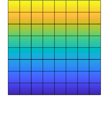
(a) A $9\times 9$ grid graph

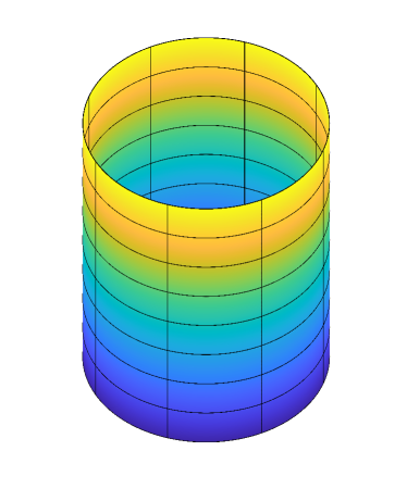
(b) An $8\times 9$ cylinder grid graph

Figure 1: The figures of a grid graph and a cylinder grid graph.

2.2 Problem formulation

The Turing’s model is proposed to explain the process of biological pattern formation(cf., Turing, (1952); Maini et al., (2012)). The dynamics of the system is described by

$$\left\{\begin{array}[]{c}\frac{\partial{z}_{1}(t,x,y)}{\partial t}=\nu_{1}\Delta z_{1}+f(z_{1},z_{2}),\\ \frac{\partial{z}_{2}(t,x,y)}{\partial t}=\nu_{2}\Delta z_{2}+g(z_{1},z_{2}),\end{array}\right.$$

where $t\in[0,+\infty)$, $(x,y)\in\mathbf{D}$ with $\mathbf{D}$ being a bounded region contained in $\mathbf{R}^{2}$, $z_{i}\in\mathbf{R}$, $f,g:\mathbf{R}^{2}\rightarrow\mathbf{R}$ are two differential functions, $\Delta=\frac{\partial^{2}}{\partial x^{2}}+\frac{\partial^{2}}{\partial y^{2}}$ is the Laplace operator in $\mathbf{R}^{2}$, and $\nu_{1},\nu_{2}$ are two positive constants. Appropriate boundary and initial conditions are applied to close the system. In the Turing’s model, ${z}_{i}(t,x,y)$ represents concentrations of chemical material $\mathbf{M}_{i}$ at time $t$ and location $(x,y)$. $\nu_{1}\Delta z_{1}$ and $\nu_{2}\Delta z_{2}$ represent diffusion rates of chemical materials $\mathbf{M}_{1}$ and $\mathbf{M}_{2}$, respectively, and $\nu_{1}$ and $\nu_{2}$ are diffusion coefficients. $f(z_{1},z_{2})$ and $g(z_{1},z_{2})$ are the production rates or consumption rates of $\mathbf{M}_{1}$ and $\mathbf{M}_{2}$ by chemical reaction.

This model is described by nonlinear partial differential equations, whose dynamics are hard to analyze. To simplify this model, we first discretize the region $\mathbf{D}$ into a graph of $N$ vertexes. Then, by linearization and spatial discretization (sampling on vertexes of the graph in $\mathbf{D}$), we get the following linear second-order multi-agent system,

$$\left\{\begin{array}[]{c}\dot{z}_{1}(t)=-\nu_{1}Lz_{1}+az_{1}+bz_{2},\\ \dot{z}_{2}(t)=-\nu_{2}Lz_{2}+cz_{1}+dz_{2},\end{array}\right.$$

where $L$ is the Laplacian matrix of the graph, $z_{i}(t)=[z_{i}^{(1)},\cdots,z_{i}^{(N)}]\in\mathbf{R}^{N}$ denotes the concentration of $M_{i}$ at sampling points for $i=1,2$. Each vertex $j\ (1\leq j\leq N)$, also called agent, has two states $z^{(j)}_{1}$ and $z^{(j)}_{2}$. Few patterns will emerge if the above linear system evolves in a self-organization manner. We are interested in whether it is possible to generate desired patterns by external intervention. Thus, we choose $\kappa+\tau$ states $z^{(i_{1})}_{1},\cdots,z^{(i_{\kappa})}_{1},z^{(j_{1})}_{2},\cdots,z^{(j_{\tau})}_{2}$ to add control. By this way, we can obtain the following controlled linearized Turing’s model,

$$\left\{\begin{array}[]{c}\dot{z}_{1}(t)=-\nu_{1}Lz_{1}+az_{1}+bz_{2}+Bu_{1},\\ \dot{z}_{2}(t)=-\nu_{2}Lz_{2}+cz_{1}+dz_{2}+Cu_{2},\end{array}\right.$$ (1)

where $L$ is the Laplacian matrix of a graph, $\nu_{1},\nu_{2}>0$, $a,b,c,d\in\mathbf{R}$, $z_{i}(t)\in\mathbf{R}^{N}$ for $i=1,2$ and $t\in[0,+\infty)$, $B=[e^{(N)}_{i_{1}},\cdots,e^{(N)}_{i_{\kappa}}]$ and $C=[e^{(N)}_{j_{1}},\cdots,e^{(N)}_{j_{\tau}}]$ ( $1\leq i_{k},j_{l}\leq N$ for $1\leq k\leq\kappa$ and $1\leq l\leq\tau$) are control matrices, $e^{(N)}_{j}$ denotes the $j$th column of $N\times N$ unit matrix, $u_{1}\in\mathbf{R}^{\kappa}$ and $u_{2}\in\mathbf{R}^{\tau}$ are the control inputs.

If system (1) is controllable, then the desired behaviors can be achieved by designing control inputs. In this paper, we will investigate how to choose control matrices $B$ and $C$ to achieve controllability of the system.

In the controlled linearized Turing’s model (1), by choosing some states instead of vertexes to add control, we can reduce the amount of controlled states to achieve controllability of the system. We illustrate this point by an example.

Example 1.

Let the parameters in system (1) be taken as $\nu_{1}=\nu_{2}=1$, $a=1$, $b=2$, $c=3$, $d=4$. The number of vertexes is $N=3$, and the graph is taken as a path graph with the corresponding Laplacian matrix

$$L=\begin{bmatrix}1&-1&0\\ -1&2&-1\\ 0&-1&1\end{bmatrix}.$$

If we choose vertexes to add control, then we can achieve controllability of the system by controlling the first vertex. For this case, the control matrices are $B=C=e^{(3)}_{1}$, and two states $z^{(1)}_{1}$ and $z^{(1)}_{2}$ are controlled. On the other hand, if we choose states to add control, then we only need to choose the first state of the first vertex, i.e. $z^{(1)}_{1}$, to achieve controllability of the system. The control matrices are $B=e^{(3)}_{1}$ and $C=0$.

3 Controllability of the linearized Turing’s model

Denote

$$A=\begin{bmatrix}-\nu_{1}L+aI&bI\\ cI&-\nu_{2}L+dI\end{bmatrix},$$

$$\tilde{B}=\begin{bmatrix}B&0_{N\times\tau}\\ 0_{N\times\kappa}&C\end{bmatrix}.$$

Then (1) can be written as

$$\dot{z}=Az+\tilde{B}u,$$

where $z=[z_{1}^{T},z_{2}^{T}]^{T}$ and $u=[u_{1}^{T},u_{2}^{T}]^{T}$.

We first give a necessary condition for the controllability of $(A,\tilde{B})$.

Lemma 1.

If $(A,\tilde{B})$ is controllable, then $(L,\begin{bmatrix}B&C\end{bmatrix})$ is controllable.

Proof.

If $(L,\begin{bmatrix}B&C\end{bmatrix})$ is uncontrollable, then by PBH criterion (Bacciotti, (2019)), there exist $\lambda\in\mathbf{C}$ and a nonzero vector $v\in\mathbf{C}^{N}$ such that $v^{T}L=\lambda v^{T}$, and $v^{T}B=v^{T}C=0$. By calculation, we can derive that $[v^{T},0_{1\times N}]A^{k}\tilde{B}=0$ for $k=0,1,...,N-1$, which indicates that $(A,\tilde{B})$ is uncontrollable. By reduction to absurdity, the lemma is proved. ∎

In the following, we consider the sufficient conditions for the controllability of $(A,\tilde{B})$. Since both the analysis and results for the controllability of $(A,\tilde{B})$ are different for the cases of $C=B$ and $C\neq B$, we will study these two cases separately. We first provide a necessary and sufficient condition for the controllability of $(A,\tilde{B})$ when $C=B$.

Proposition 1.

If $\nu_{1}\neq 0,\nu_{2}\neq 0$ and $C=B$, then $(A,\tilde{B})$ is controllable if and only if $(L,B)$ is controllable.

Proof.

By Lemma 1, we have the necessity. Now, we consider the sufficiency. Denote

$$B_{1}=\begin{bmatrix}B\\ 0_{N\times\kappa}\end{bmatrix},B_{2}=\begin{bmatrix}0_{N\times\kappa}\\ B\end{bmatrix},$$

$$F=\begin{bmatrix}aI&bI\\ cI&dI\end{bmatrix},\bar{L}=\begin{bmatrix}L&0_{N\times\kappa}\\ 0_{N\times\kappa}&L\end{bmatrix}.$$

We have for $k\in\mathbf{N}$,

$$A\bar{L}^{k}B_{1}= -\nu_{1}\bar{L}^{k+1}B_{1}+F\bar{L}^{k}B_{1}$$

$$=-\nu_{1}\bar{L}^{k+1}B_{1}+a\bar{L}^{k}B_{1}+c\bar{L}^{k}B_{2},$$ (2)

and

$$A\bar{L}^{k}B_{2} =-\nu_{2}\bar{L}^{k+1}B_{2}+F\bar{L}^{k}B_{2}$$

$$=-\nu_{2}\bar{L}^{k+1}B_{2}+b\bar{L}^{k}B_{1}+d\bar{L}^{k}B_{2}.$$ (3)

We claim that for $k\in\mathbf{Z}^{+}$,

$$A^{k}B_{1}=(-\nu_{1})^{k}\bar{L}^{k}B_{1}+\sum_{i=1}^{k}(p_{ik}\bar{L}^{i-1}B_{1}+q_{ik}\bar{L}^{i-1}B_{2}),$$ (4)

$$A^{k}B_{2}=(-\nu_{2})^{k}\bar{L}^{k}B_{2}+\sum_{i=1}^{k}(r_{ik}\bar{L}^{i-1}B_{1}+t_{ik}\bar{L}^{i-1}B_{2}),$$ (5)

where $p_{ik}$, $q_{ik}$, $r_{ik}$ and $t_{ik}$ are some proper real numbers. We prove equations (4) and (5) by induction. It is clear that the equations hold for $k=1$. We assume that equations (4) and (5) hold for $k\leq m$. Then for $k=m+1$, by (2) and (3), we have

$$A^{m+1}B_{1}=A(A^{m}B_{1})$$

$$=(-\nu_{1})^{m}A\bar{L}^{m}B_{1}+\sum_{i=1}^{m}(p_{im}A\bar{L}^{i-1}B_{1}+q_{im}A\bar{L}^{i-1}B_{2})$$

$$=(-\nu_{1})^{m+1}\bar{L}^{m+1}B_{1}$$

$$+\sum_{i=1}^{m+1}(p_{i,m+1}\bar{L}^{i-1}B_{1}+q_{i,m+1}\bar{L}^{i-1}B_{2}),$$

$$A^{m+1}B_{2}=A(A^{m}B_{2})$$

$$=(-\nu_{2})^{m}A\bar{L}^{m}B_{2}+\sum_{i=1}^{m}(r_{im}A\bar{L}^{i-1}B_{1}+t_{im}A\bar{L}^{i-1}B_{2})$$

$$=(-\nu_{2})^{m+1}\bar{L}^{m+1}B_{2}$$

$$+\sum_{i=1}^{m+1}(r_{i,m+1}\bar{L}^{i-1}B_{1}+t_{i,m+1}\bar{L}^{i-1}B_{2}),$$

where

$$p_{m+1,m+1}=(-\nu_{1})^{m}a-\nu_{1}p_{m,m},$$

$$p_{i,m+1}=ap_{i,m}+bq_{i,m}-\nu_{1}p_{i-1,m},$$

$$p_{1,m+1}=ap_{1,m}+bq_{1,m},$$

$$q_{m+1,m+1}=(-\nu_{1})^{m}c-\nu_{2}q_{m,m},$$

$$q_{i,m+1}=cp_{i,m}+dq_{i,m}-\nu_{2}q_{i-1,m},$$

$$q_{1,m+1}=cp_{1,m}+dq_{1,m},$$

$$r_{m+1,m+1}=(-\nu_{2})^{m}b-\nu_{1}r_{m,m},$$

$$r_{i,m+1}=ar_{i,m}+bt_{i,m}-\nu_{1}r_{i-1,m},$$

$$r_{1,m+1}=ar_{1,m}+bt_{1,m},$$

$$t_{m+1,m+1}=(-\nu_{2})^{m}d-\nu_{2}t_{m,m},$$

$$t_{i,m+1}=cr_{i,m}+dt_{i,m}-\nu_{2}t_{i-1,m},$$

$$t_{1,m+1}=cr_{1,m}+dt_{1,m},$$

for $2\leq i\leq m$. Thus, equations (4) and (5) hold. By (4) and (5), we have

$$[B_{1},B_{2},AB_{1},AB_{2},\cdots,A^{2N-1}B_{1},A^{2N-1}B_{2}]$$

$$=[B_{1},B_{2},\bar{L}B_{1},\bar{L}B_{2},\cdots,\bar{L}^{2N-1}B_{1},\bar{L}^{2N-1}B_{2}]Q,$$

where $Q$ is a $4N\kappa\times 4N\kappa$ invertible matrix. Thus we have

$$rank([B_{1},B_{2},AB_{1},AB_{2},\cdots,A^{2N-1}B_{1},A^{2N-1}B_{2}])$$

$$=rank[B_{1},B_{2},\bar{L}B_{1},\bar{L}B_{2},\cdots,\bar{L}^{2N-1}B_{1},\bar{L}^{2N-1}B_{2}]$$

$$=2\times rank([B,LB,\cdots,L^{N-1}B])$$

$$=2N,$$

which indicates that $(A,\tilde{B})$ is controllable. ∎

Next, we consider the case of $C\neq B$. Since the equations (2) and (3) do not hold when $C\neq B$, the method used in Proposition 1 is not applicable for such a case. We focus on analyzing the relationship of eigenvalues and eigenvectors between matrices $A$ and $L$. According to the definition of $A$, if $L$ has an eigenvalue $\lambda$ with left eigenvector $v^{T}$, then $A$ has two eigenvalues $s_{i}(\lambda)(i=1,2)$ and two left eigenvectors $[v^{T},k_{i}(\lambda)v^{T}](i=1,2)$, where $s_{i}(\lambda)(i=1,2)$ are roots of the following equation

$$s^{2}-((-\nu_{1}\lambda+a)+(-\nu_{2}\lambda+d))s$$ (6)

$$+((-\nu_{1}\lambda+a)(-\nu_{2}\lambda+d)-bc)=0,$$

and $k_{i}(\lambda)(i=1,2)$ are the roots of the equation

$$ck^{2}+((\nu_{2}-\nu_{1})\lambda+(a-d))k-b=0.$$ (7)

By simple calculations, the roots of (6) are

$$s_{1}(\lambda)=\frac{((-\nu_{1}\lambda+a)+(-\nu_{2}\lambda+d))+\sqrt{\Delta}}{2},$$

$$s_{2}(\lambda)=\frac{((-\nu_{1}\lambda+a)+(-\nu_{2}\lambda+d))-\sqrt{\Delta}}{2},$$

and the roots of (7) are

$$k_{1}(\lambda)=\frac{-((\nu_{2}-\nu_{1})\lambda+(a-d))+\sqrt{\Delta}}{2c},$$

$$k_{2}(\lambda)=\frac{-((\nu_{2}-\nu_{1})\lambda+(a-d))-\sqrt{\Delta}}{2c},$$

where $\Delta=\Delta(\lambda)=((\nu_{2}-\nu_{1})\lambda+(a-d))^{2}+4bc.$

Denote $S=S_{1}\cup S_{2}$ with

$$S_{1}=\Big{\{}(a,b,c,d,\nu_{1},\nu_{2})\in\mathbf{R}^{6}|there\ exist\ j,l\in\{1,2\},$$ (8)

$$\lambda_{1},\lambda_{2}\in\sigma(L),\lambda_{1}\neq\lambda_{2},such\ that\ s_{j}(\lambda_{1})=s_{l}(\lambda_{2})\Big{\}},$$

and

$$S_{2}=\Big{\{} (a,b,c,d,\nu_{1},\nu_{2})\in\mathbf{R}^{6}|there\ exists\ \lambda\in\sigma(L),$$ (9)

$$such\ that\ \Delta(\lambda)=0\Big{\}},$$

where $\sigma(L)=\{\lambda_{i}|1\leq i\leq N\}$ is the spectrum of $L$. It is clear that $\mathbf{m}(S)=0$, where $\mathbf{m}(\cdot)$ is the Lebesgue measure in $\mathbf{R}^{6}$.

Proposition 2.

If $(a,b,c,d,\nu_{1},\nu_{2})\in\mathbf{R}^{6}-S$, $b\neq 0$, and $c\neq 0$, then $(A,\tilde{B})$ is controllable if and only if $(L,\begin{bmatrix}B&C\end{bmatrix})$ is controllable.

Proof.

By Lemma 1, we have necessity. Now, we consider sufficiency. By $b\neq 0$, $c\neq 0$ and $(a,b,c,d,\nu_{1},\nu_{2})\notin S_{2}$, the equation (7) has two different nonzero roots $k_{j}(\lambda)(j=1,2)$, where $S_{2}$ is defined in (9). The set of left eigenvectors of $A$, i.e., $\{[v^{T},k_{j}(\lambda)v^{T}]|\lambda\in\sigma(L),v^{T}L=\lambda v^{T},j=1,2\}$, constructs a basis of $\mathbf{R}^{2N}$. For a given eigenvalue $s_{0}$ of $A$, each left eigenvectors $w^{T}$ can be expressed as

$$w^{T}=\sum_{i=1}^{N}\sum_{j=1}^{2}l_{ij}[v_{i}^{T},k_{j}(\lambda_{i})v_{i}^{T}].$$ (10)

By $w^{T}A=s_{0}w^{T}$, we can deduce that for $1\leq i\leq N$ and $j=1,2$

$$l_{ij}=0,\ if\ s_{j}(\lambda_{i})\neq s_{0}.$$ (11)

By the condition $(a,b,c,d,\nu_{1},\nu_{2})\notin S_{2}$, we have $s_{1}(\lambda_{i})\neq s_{2}(\lambda_{i})$ for $1\leq i\leq N$. Based on (11), we have $l_{i1}=0$ or $l_{i2}=0$ for $1\leq i\leq N$ by reduction to absurdity. Without loss of generality, we assume that $l_{i2}=0$ for $1\leq i\leq N$, $s_{1}(\lambda_{i})=s_{0}$ for $1\leq i\leq p(1\leq p\leq N)$, and $l_{i1}=0$ for $p+1\leq i\leq N$. As $s_{1}(\lambda_{1})=\cdots=s_{1}(\lambda_{p})=s_{0}$ and $(a,b,c,d,\nu_{1},\nu_{2})\notin S_{1}$, we have $\lambda_{1}=\cdots=\lambda_{p}$ and $k_{j}(\lambda_{1})=\cdots=k_{j}(\lambda_{p})\triangleq k_{j}(j=1,2)$, where $S_{1}$ is defined in (8). Then by (10) and the above assumption, we have $w^{T}=[u^{T},k_{1}u^{T}]$, where $u=\sum_{i=1}^{p}l_{i1}v_{i}$ is a left eigenvector of $L$ subject to the eigenvalue $\lambda_{1}$. Thus, every left eigenvector can be expressed as the form of $[v^{T},lv^{T}]$, where $v^{T}$ is a left eigenvector of $L$ and $l\in\mathbf{C},l\neq 0$.

If $(A,\tilde{B})$ is uncontrollable, then by PBH criterion, there exists a left eigenvector $[v^{T},lv^{T}]$ such that $[v^{T},lv^{T}]\tilde{B}=0$, where $v^{T}$ is a left eigenvector of $L$. Thus, we have $v^{T}\begin{bmatrix}B&C\end{bmatrix}=0$, which indicates that $(L,\begin{bmatrix}B&C\end{bmatrix})$ is uncontrollable. By reduction to absurdity, the sufficiency is proved. ∎

For both cases $B=C$ and $B\neq C$, we have proved that the controllability of $(A,\tilde{B})$ is equivalent to the controllability of $(L,\begin{bmatrix}B&C\end{bmatrix})$ except for a set of zero Lebesgue measure. By now, the controllability problem of a second-order multiagent system is transferred to that of a first-order multiagent system. Thus, the analysis of the controllability problem can be simplified.

In the following section, we investigate the controllability of $(L,\bar{B})$ with $\bar{B}=\begin{bmatrix}B&C\end{bmatrix}$.

4 Controllability of $(L,\bar{B})$

In this section, we consider controllability of the system

$$\dot{z}=Lz+\bar{B}u,$$ (12)

where $z\in\mathbf{R}^{N}$, $u\in\mathbf{R}^{\rho}$, $L$ is the Laplacian matrix of the graph, $\bar{B}=[e^{(N)}_{i_{1}},\cdots,e^{(N)}_{i_{\rho}}]$ is the control matrix with $1\leq i_{k}\leq N(1\leq k\leq\rho)$ and $\rho$ is the number of controlled nodes. For general graphs, it is hard to give a detailed analysis for the controllability of the system (12) since eigenvalues and eigenvectors of $L$ can not be explicitly expressed. Thus, we consider the controllability on two typical graphs: grid graph and cylinder grid graph, which are shown in Fig. 1.

A direct lemma derived from PBH Criterion is introduced, which gives a necessary condition for the controllability of $(L,\bar{B})$.

Lemma 2.

If $L$ has an eigenvalue with multiplicity $r$ and $rank(\bar{B})<r$, then $(L,\bar{B})$ is uncontrollable.

4.1 Controllability of system (12) on grid graphs

In this subsection, we consider controllability of the system (12) on $m\times n$ grid graphs $\mathcal{L}_{m,n}$, and the Laplacian matrix of $\mathcal{L}_{m,n}$ is denoted as $L(m,n)$.

We know that the grid graph $\mathcal{L}_{m,n}$ is the Cartesian product of two path graphs $\mathcal{P}_{m}$ and $\mathcal{P}_{n}$, and we first introduce a lemma which gives the explicit expression of eigenvalues and eigenvectors of the Laplacian matrix $L_{\mathcal{P}}(m)$ of the path graph $\mathcal{P}_{m}$.

Lemma 3 (Yueh, (2005)).

The eigenvalues $\lambda^{(\mathcal{P})}_{0},\cdots,$ $\lambda^{(\mathcal{P})}_{m-1}$ of $L_{\mathcal{P}}(m)$ are given by

$$\lambda^{(\mathcal{P})}_{\alpha}=2-2\cos{\frac{\alpha\pi}{m}},\ \alpha=0,1,\cdots,m-1,$$

and the corresponding eigenvectors $v_{\alpha}=[v_{\alpha,1},\cdots,v_{\alpha,m}]^{T}$ are given by

$$v_{\alpha,k}=\begin{cases}\frac{1}{\sqrt{m}},&\mbox{if $\alpha=0$;}\\ \sqrt{\frac{2}{m}}\cos{\frac{\alpha(2k-1)\pi}{2m}},&\mbox{otherwise;}\end{cases}$$ (13)

for $k=1,2,\cdots,m$.

Based on the above lemma, we have the following results about the eigenvalues and eigenvectors of the Laplacian matrix $L(m,n)$ of the grid graph $\mathcal{L}_{m,n}$.

Lemma 4.

$L(m,n)$ has the following $mn$ eigenvalues,

$$\lambda_{\alpha\beta}=4-2\big{(}\cos{\frac{\alpha\pi}{m}}+\cos{\frac{\beta\pi}{n}}\big{)},0\leq\alpha\leq m-1,0\leq\beta\leq n-1.$$ (14)

The eigenvector subject to $\lambda_{\alpha\beta}$ is $v_{\alpha}\otimes w_{\beta}$, where $\otimes$ denotes the Kronecker product, $v_{\alpha}=[v_{\alpha,1},\cdots,v_{\alpha,m}]^{T}$ with $v_{\alpha,k}$ defined in (13) and $w_{\beta}=[w_{\beta,1},\cdots,w_{\beta,m}]^{T}$ with

$$w_{\beta,l}=\begin{cases}\frac{1}{\sqrt{n}},&\mbox{if $\beta=0$;}\\ \sqrt{\frac{2}{n}}\cos{\frac{\beta(2l-1)\pi}{2n}},&\mbox{otherwise;}\end{cases}$$ (15)

for $1\leq l\leq n$.

From (14), we see that “$\cos{\frac{\alpha\pi}{m}}+\cos{\frac{\beta\pi}{n}}$” reflects the difference between $\lambda_{\alpha\beta}$ with other eigenvalues, so we call $\cos{\frac{\alpha\pi}{m}}+\cos{\frac{\beta\pi}{n}}$ the characteristic part of $\lambda_{\alpha\beta}$. Denote $V=[v_{0},\cdots,v_{m-1}]^{T}$ and $W=[w_{0},\cdots,w_{n-1}]^{T}$.

Remark 1.

Since $\{v_{\alpha}\}_{0\leq\alpha\leq m-1}$ are unit eigenvectors subject to different eigenvalues of $L_{\mathcal{P}}(m)$, $V$ is an orthogonal matrix. Similarly, $W$ is an orthogonal matrix.

We first consider the case of $m=n$. We denote $L(n,n)$ as the Laplacian matrix of the grid graph $\mathcal{L}_{n,n}$. Based on Lemma 4, we have the following result on the largest multiplicity of the eigenvalues of $L(n,n)$.

Corollary 1.

For $n\geq 3$, the largest multiplicity of eigenvalues of $L(n,n)$ is $n-1$.

Proof.

By Lemma 4, for $\beta=n-\alpha$ with $1\leq\alpha\leq n-1$, we have $\lambda_{\alpha\beta}=4$. Thus, $L(n,n)$ has an eigenvalue with multiplicity $n-1$. In the following, we show that $L(n,n)$ has no eigenvalues whose multiplicities are strictly larger than $n-1$ by reduction to absurdity. If $L(n,n)$ has an eigenvalue whose multiplicity is larger than $n-1$, then there exist two sequences $\{\alpha_{i},0\leq\alpha_{i}\leq n-1\}_{0\leq i\leq n-1}$ and $\{\beta_{i},0\leq\beta_{i}\leq n-1\}_{0\leq i\leq n-1}$ such that

$$\lambda_{\alpha_{0},\beta_{0}}=\lambda_{\alpha_{1},\beta_{1}}=\cdots=\lambda_{\alpha_{n-1},\beta_{n-1}},$$ (16)

where $\alpha_{i}\neq\alpha_{j}$ and $\beta_{i}\neq\beta_{j}$ for any $0\leq i<j\leq n-1$.

Without loss of generality, we assume that $\alpha_{0}<\alpha_{1}<\cdots<\alpha_{n-1}$. Then by (14) and (16), we have $\beta_{0}>\beta_{1}>\cdots>\beta_{n-1}$. Thus, for $0\leq i\leq n-1$, we have $\alpha_{i}=n-1-\beta_{i}=i$. By the first equation in (16), we have $1+\cos{\frac{2\pi}{n}}=2\cos{\frac{\pi}{n}}$, which contradicts with the fact $1+\cos{\frac{2\pi}{n}}=2\cos^{2}{\frac{\pi}{n}}<2\cos{\frac{\pi}{n}}$. This completes the proof of Corollary 1. ∎

We next introduce a lemma about orthogonal matrices, which will be used in the proof of the following theorems.

Lemma 5 (Horn and Johnson, (2012)).

Let $W=(w_{ij})_{n\times n}$ be an orthogonal matrix. Denote

$$W^{*}_{ij}=\begin{bmatrix}w_{11}&\cdots&w_{1,j-1}&w_{1,j+1}&\cdots&w_{1,n}\\ \vdots&\ddots&\vdots&\vdots&\ddots&\vdots\\ w_{i-1,1}&\cdots&w_{i-1,j-1}&w_{i-1,j+1}&\cdots&w_{i-1,n}\\ w_{i+1,1}&\cdots&w_{i+1,j-1}&w_{i+1,j+1}&\cdots&w_{i+1,n}\\ \vdots&\ddots&\vdots&\vdots&\ddots&\vdots\\ w_{n,1}&\cdots&w_{n,j-1}&w_{n,j+1}&\cdots&w_{n,n}\end{bmatrix}.$$ (17)

Then for $1\leq i,j\leq n$, $det(W^{*}_{ij})=0$ if and only if $w_{ij}=0$.

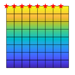
Figure 2: This figure illustrates how to choose control nodes on the grid graph $\mathcal{L}_{m,n}$ such that $(L(m,n),\bar{B})$ is controllable for $m=n$, where the control nodes are marked by red stars.

Now, we give a theorem about the minimal number of control nodes such that $(L(n,n),\bar{B})$ is controllable. The meaning of “minimal number” is twofold. One is that there exist at least a set of control nodes whose cardinality is exactly the given minimal number such that $(L(n,n),\bar{B})$ is controllable. Another is that if the number of control nodes is less than the given minimal number, then $(L(n,n),\bar{B})$ is uncontrollable no matter how we choose control nodes.

Theorem 1.

Denote $\varphi(n,n)$ as the minimal number of control nodes such that $(L(n,n),\bar{B})$ is controllable, that is,

$$\varphi(n,n)=\min\big{\{}\rho\in\mathbf{Z}^{+}|there\ exist\ i_{1},...,i_{\rho},\ 1\leq i_{1},...,i_{\rho}$$

$$\leq n^{2},\ such\ that\ (L(n,n),[e^{(n^{2})}_{i_{1}},\cdots,e^{(n^{2})}_{i_{\rho}}])\ is$$

$$controllable\big{\}}.$$

Then we have

$$\varphi(n,n)=\begin{cases}n,&\mbox{for $n=1,2$;}\\ $n$-1,&\mbox{for $n\geq 3$.}\end{cases}$$

Proof.

For $n=1,2$, it is clear that $\varphi(n,n)=n$ by directly calculating the rank of controllability matrices.

For $n\geq 3$, by Lemma 2 and Corollary 1, we have $\varphi(n,n)\geq n-1$. In the following, we prove $\varphi(n,n)\leq n-1$. We choose the first $n-1$ nodes in the first row as control nodes as illustrated in Fig. 2. It is clear that the corresponding control matrix is

$$\bar{B}=e^{(n)}_{1}\otimes[e^{(n)}_{1},\cdots,e^{(n)}_{n-1}].$$

By Lemma 4, for any eigenvalue of $L(n,n)$ with multiplicity $r$, there exist two sequences $\{\alpha_{i},0\leq\alpha_{i}\leq n-1\}_{1\leq i\leq r}$ and $\{\beta_{i},0\leq\beta_{i}\leq n-1\}_{1\leq i\leq r}$ such that

$$\lambda_{\alpha_{1},\beta_{1}}=\lambda_{\alpha_{2},\beta_{2}}=\cdots=\lambda_{\alpha_{r},\beta_{r}},$$

where $\lambda_{\alpha,\beta}$ is defined in Lemma 4, and $\alpha_{i}\neq\alpha_{j}$ and $\beta_{i}\neq\beta_{j}$ for any $1\leq i<j\leq r$. By Corollary 1, we have $r\leq n-1$. Denote any one of the eigenvectors corresponding to the above eigenvalue as $u$, then there exists a vector $g=[g_{1},\cdots,g_{r}]^{T}\in\mathbf{R}^{r}\backslash\{0\}$, such that $u=\sum_{i=1}^{r}g_{i}(v_{\alpha_{i}}\otimes w_{\beta_{i}})$, where $v_{\alpha_{i}}$ and $w_{\beta_{i}}$ are defined in Lemma 4. By PBH criterion, we need to show $u^{T}\bar{B}\neq 0$ for any $g\neq 0$.

By Lemma 5, Remark 1 and the fact that $w_{\beta,n}\neq 0$ for any $0\leq\beta\leq n-1$, we have $rank(W^{*}_{\beta,n})=n-1$, where $w_{\beta,n}$ is defined in (15) and $W^{*}_{\beta,n}$ is defined in (17). As $r\leq n-1$, we have

$$rank\left(\begin{bmatrix}w_{\beta_{1},1}&\cdots&w_{\beta_{1},n-1}\\ \vdots&\ddots&\vdots\\ w_{\beta_{r},1}&\cdots&w_{\beta_{r},n-1}\end{bmatrix}\right)=r.$$

Thus, we have

$$rank\left(\begin{bmatrix}(v_{\alpha_{1}}\otimes w_{\beta_{1}})^{T}\bar{B}\\ \vdots\\ (v_{\alpha_{r}}\otimes w_{\beta_{r}})^{T}\bar{B}\end{bmatrix}\right)$$

$$=rank\left(\begin{bmatrix}w_{\beta_{1},1}&\cdots&w_{\beta_{1},n-1}\\ \vdots&\ddots&\vdots\\ w_{\beta_{r},1}&\cdots&w_{\beta_{r},n-1}\end{bmatrix}\right)=r.$$

This indicates $u^{T}\bar{B}=\sum_{i=1}^{r}g_{i}(v_{\alpha_{i}}\otimes w_{\beta_{i}})^{T}\bar{B}\neq 0$ for any $g\neq 0$. Thus, system (12) is controllable by choosing control nodes in the above manner. We complete the proof of the theorem. ∎

In the following, we consider the case of $m\neq n$. Firstly, we introduce a lemma which gives the complete solution of the following trigonometric diophantine equation

$$\cos{(f_{1}\pi)}+\cos{(f_{2}\pi)}+\cos{(f_{3}\pi)}+\cos{(f_{4}\pi)}=0,$$ (18)

in which all the variables $f_{j}(0\leq f_{j}\leq 1,1\leq j\leq 4)$ are rational. In the following lemma, we express a solution of (18) by an unordered quadruple $\{f_{1},f_{2},f_{3},f_{4}\}$.

Lemma 6 (Wlodarski, (1969)).

If rational numbers $f_{j}(0\leq f_{j}\leq 1,1\leq j\leq 4)$ satisfy the trigonometric diophantine equation (18), then $\{f_{1},f_{2},f_{3},f_{4}\}$ either belongs to the following infinite family (19) or (20)

$$\left\{\gamma,\delta,\pi-\gamma,\pi-\delta\right\}\ \left(0\leq\gamma\leq\delta\leq\frac{\pi}{2}\right),$$ (19)

$$\left\{\theta,\frac{2\pi}{3}-\theta,\frac{2\pi}{3}+\theta,\frac{\pi}{2}\right\}\ \left(0<\theta<\frac{\pi}{3}\right)$$ (20)

or is one of the following quadruples

$$\left\{\frac{\pi}{3},\pi,\frac{\pi}{2},\frac{\pi}{3}\right\},\ \left\{\frac{2\pi}{3},0,\frac{\pi}{2},\frac{2\pi}{3}\right\},$$ (21)

$$\left\{\frac{2\pi}{5},\frac{4\pi}{5},\frac{\pi}{2},\frac{\pi}{3}\right\},\ \left\{\frac{3\pi}{5},\frac{\pi}{5},\frac{\pi}{2},\frac{2\pi}{3}\right\},$$

$$\left\{\frac{\pi}{5},\frac{3\pi}{5},\pi,\frac{\pi}{3}\right\},\ \left\{\frac{4\pi}{5},\frac{2\pi}{5},0,\frac{2\pi}{3}\right\},$$

$$\left\{\frac{2\pi}{5},\frac{7\pi}{15},\frac{13\pi}{15},\frac{\pi}{3}\right\},\ \left\{\frac{3\pi}{5},\frac{8\pi}{15},\frac{2\pi}{15},\frac{2\pi}{3}\right\},$$

$$\left\{\frac{\pi}{15},\frac{4\pi}{5},\frac{11\pi}{15},\frac{\pi}{3}\right\},\ \left\{\frac{14\pi}{15},\frac{\pi}{5},\frac{4\pi}{15},\frac{2\pi}{3}\right\},$$

$$\left\{\frac{2\pi}{7},\frac{4\pi}{7},\frac{6\pi}{7},\frac{\pi}{3}\right\},\ \left\{\frac{5\pi}{7},\frac{3\pi}{7},\frac{\pi}{7},\frac{2\pi}{3}\right\}.$$

Denote $L(m,n)$ as the Laplacian matrix of the grid graph $\mathcal{L}_{m,n}$. By Lemma 6, we can obtain the largest multiplicity of eigenvalues of $L(m,n)$ for general $m$ and $n$.

Corollary 2.

Let $\psi(m,n)$ denote the largest multiplicity of eigenvalues of $L(m,n)$, and $\mathbf{d}$ denote the greatest common divisor of $m$ and $n$. Then we have

• for $\mathbf{d}\geq 4$, $\psi(m,n)=\mathbf{d}-1$;

• for $\mathbf{d}=3$,

  $$\psi(m,n)=\begin{cases}3,&\mbox{if $2|m$ or $2|n$;}\\ 2,&\mbox{otherwise;}\end{cases}$$

• for $\mathbf{d}=2$, $\psi(m,n)=2$;

• for $\mathbf{d}=1$,

  $$\psi(m,n)=\begin{cases}2,&\mbox{if $(2|m,3|n)$ or $(3|m,2|n)$}\\ &\mbox{or $(3|m,5|n)$ or $(5|m,3|n)$;}\\ 1,&\mbox{otherwise;}\end{cases}$$

where $p|q$ denotes that $p$ divides $q$ exactly, and $(2|m,3|n)$ means that these two conditions $2|m$ and $3|n$ are satisfied simultaneously.

Proof.

By Lemma 4, we need to solve the following trigonometric diophantine equation in order to find all the multiple eigenvalues of $L(m,n)$,

$$\cos{\frac{\alpha_{1}\pi}{m}}+\cos{\frac{\beta_{1}\pi}{n}}=\cos{\frac{\alpha_{2}\pi}{m}}+\cos{\frac{\beta_{2}\pi}{n}},$$ (22)

where $\alpha_{i}(i=1,2)\in\{0,1,\cdots,m-1\}$ and $\beta_{i}(i=1,2)\in\{0,1,\cdots,n-1\}$. The solutions of (22) are given by (19)(20) and (21) in Lemma 6.

We further discuss the solutions given by (19), that is,

$$\left\{\frac{\alpha_{1}\pi}{m},\frac{\beta_{1}\pi}{n},\pi-\frac{\alpha_{2}\pi}{m},\pi-\frac{\beta_{2}\pi}{n}\right\}=\left\{\gamma,\delta,\pi-\gamma,\pi-\delta\right\},$$ (23)

where $0\leq\gamma\leq\delta\leq\frac{\pi}{2}$. The equation (23) indicates that in the unordered quadruple $\left\{\frac{\alpha_{1}\pi}{m},\frac{\beta_{1}\pi}{n},\pi-\frac{\alpha_{2}\pi}{m},\pi-\frac{\beta_{2}\pi}{n}\right\}$, there exist two terms whose sum is $\pi$ and sum of the other two terms is also $\pi$. If $\frac{\alpha_{1}\pi}{m}+\frac{\beta_{1}\pi}{n}=\pi$, then the solutions of (22) are

$$\alpha_{i}=\frac{k_{i}m}{\mathbf{d}},\ \beta_{i}=\frac{(\mathbf{d}-k_{i})n}{\mathbf{d}}$$ (24)

for $i=1,2$ and $1\leq k_{i}\leq\mathbf{d}-1$. If $\frac{\alpha_{1}\pi}{m}+(\pi-\frac{\alpha_{2}\pi}{m})=\pi,$ then we have $\alpha_{1}=\alpha_{2}$ and $\beta_{1}=\beta_{2}$. If $\frac{\alpha_{1}\pi}{m}+(\pi-\frac{\beta_{2}\pi}{n})=\pi,$ then the solutions of (22) are

$$\alpha_{i}=\frac{k_{i}m}{\mathbf{d}},\ \beta_{3-i}=\frac{k_{i}n}{\mathbf{d}}$$

for $i=1,2$ and $1\leq k_{i}\leq\mathbf{d}-1$. Solutions of (22) given in (20) and (21) can be obtained similarly. By these solutions, we can obtain all the multiple eigenvalues and corresponding multiplicities.

We see that the eigenvalue $4$ of $L(m,n)$ is of $\mathbf{d}-1$ multiplicities by (24). Thus,

$$\psi(m,n)\geq\mathbf{d}-1.$$ (25)

• For $\mathbf{d}\geq 4$, if $L(m,n)$ has an eigenvalue with multiplicity $r(r\geq 4)$, then according to the basic property of exact division and the explicit expression of solutions of (22) given in Lemma 6, we can easily deduce that

  $$\mathbf{d}-1\geq r$$ (26)

  by checking all the eigenvalues whose multiplicity is not less than 4. Now, we prove $\psi(m,n)=\mathbf{d}-1$ by reduction to absurdity. Assume that there exist $m$ and $n$ such that $\psi(m,n)>\mathbf{d}-1\geq 3$, then by (26) we have $\mathbf{d}-1\geq\psi(m,n)$. This is a contradiction. Thus, for $\mathbf{d}\geq 4$, $\psi(m,n)=\mathbf{d}-1$.

• For $\mathbf{d}=3$, by the explicit expression of solutions of (22) given in Lemma 6, we see that if $2|m$ (or $2|n$), then the only eigenvalue of $L(m,n)$ whose multiplicity is strictly larger than $\mathbf{d}-1$ has the characteristic parts $\cos{0\pi}+\cos{\frac{2\pi}{3}}=\cos{\frac{2\pi}{3}}+\cos{0\pi}=\cos{\frac{\pi}{2}}+\cos{\frac{\pi}{3}}$(or its equivalent form). Otherwise, multiplicities of all the eigenvalues of $L(m,n)$ are not more than $\mathbf{d}-1$. Thus, for $\mathbf{d}=3$, $\psi(m,n)=3$ if $2|m$ or $2|n$; otherwise, $\psi(m,n)=\mathbf{d}-1=2$.

• For $\mathbf{d}=2$, $L(m,n)$ must have an eigenvalue with multiplicity $2$, which has the following characteristic part $\cos{\frac{\pi}{2}}+\cos{0\pi}=\cos{0\pi}+\cos{\frac{\pi}{2}},$ and have no eigenvalues whose multiplicities are strictly larger than 2. Thus, for $\mathbf{d}=2$, $\psi(m,n)=2$.

• For $\mathbf{d}=1$, by the expression of solutions of (22) given in Lemma 6, we know that $L(m,n)$ has no eigenvalues whose multiplicities are strictly larger than 2. Furthermore, if ($2|m$, $3|n$) or ($3|m$, $2|n$) or ($3|m$, $5|n$) or ($5|m$, $3|n$), the eigenvalues with multiplicity 2 have at least one of the following characteristic parts or their equivalent forms

  $$\cos{\frac{\pi}{2}}+\cos{\frac{\pi}{3}}=\cos{0\pi}+\cos{\frac{2\pi}{3}},$$

  $$\cos{0\pi}+\cos{\frac{2\pi}{5}}=\cos{\frac{\pi}{3}}+\cos{\frac{\pi}{5}},$$

  $$\cos{\frac{\pi}{2}}+\cos{\frac{\pi}{5}}=\cos{\frac{\pi}{3}}+\cos{\frac{2\pi}{5}}.$$

  Thus, $\psi(m,n)=2$. Otherwise, $\psi(m,n)=1$.

This completes the proof. ∎

Based on the above corollary, we establish our theorem about the minimal number of control nodes such that $(L(m,n),\bar{B})$ is controllable when $m\neq n$.

Theorem 2.

Denote $\varphi(m,n)$ as the minimal number of control nodes such that $(L(m,n),\bar{B})$ is controllable, that is,

$$\varphi(m,n)=\min\big{\{}\rho\in\mathbf{Z}^{+}|there\ exist\ i_{1},...,i_{\rho},1\leq$$

$$i_{1},...,i_{\rho}\leq mn,\ such\ that\ (L(m,n),[e^{(mn)}_{i_{1}},\cdots,e^{(mn)}_{i_{\rho}}])$$

$$is\ controllable\big{\}}.$$

Then we have $\varphi(m,n)=\psi(m,n)$, where $\psi(m,n)$ is defined in Corollary 2.

Proof.

By Lemma 2, we see that $\varphi(m,n)\geq\psi(m,n)$. In the following, we prove $\varphi(m,n)\leq\psi(m,n)$. By Corollary 2, it is clear that $\psi(m,n)\leq\min(m,n)$. As illustrated in Fig. 3, we choose the first $\psi(m,n)$ nodes in the first row as control nodes from left to right. The corresponding control matrix is

$$\bar{B}=e^{(m)}_{1}\otimes[e^{(n)}_{1},\cdots,e^{(n)}_{\psi(m,n)}].$$

We next prove that $(L(m,n),\bar{B})$ is controllable. Similar to the proof of Theorem 1, for any eigenvalue $\lambda$ of $L(m,n)$ and the corresponding eigenvector $u$, we just need to prove

$$u^{T}\bar{B}\neq 0.$$ (27)

By the explicit expression of eigenvectors in Lemma 4, it is clear that (27) holds for any eigenvectors $u$ corresponding to single eigenvalues. In the following, we will discuss (27) for multiple eigenvalues by using Lemma 4 and Corollary 2.

We introduce a matrix $Y=[y_{i,j}]_{\mathbf{d}\times\mathbf{d}}$ whose rows are $\mathbf{d}$ eigenvectors of the Laplacian matrix of $\mathcal{P}_{\mathbf{d}}$, where $\mathbf{d}$ is the greatest common divisor of $m$ and $n$ and

$$y_{i,j}=\begin{cases}\frac{1}{\sqrt{\mathbf{d}}},&\mbox{if $i=1$;}\\ \sqrt{\frac{2}{\mathbf{d}}}\cos{\frac{(i-1)(2j-1)\pi}{2\mathbf{d}}},&\mbox{otherwise.}\end{cases}$$

Obviously, $Y$ is an orthogonal matrix. By Lemma 5 and the fact that $y_{i,\mathbf{d}}\neq 0$ for any $1\leq i\leq\mathbf{d}$, we have

$$rank(Y^{*}_{i,\mathbf{d}})=\mathbf{d}-1,$$ (28)

where $Y^{*}_{i,\mathbf{d}}$ is defined in (17).

For eigenvalues with the following characteristic parts

$$\cos{\frac{\alpha_{1}\pi}{m}}+\cos{\frac{\beta_{1}\pi}{n}}=\cdots=\cos{\frac{\alpha_{r}\pi}{m}}+\cos{\frac{\beta_{r}\pi}{n}},$$

where $r(2\leq r\leq\mathbf{d}-1)$ is the multiplicity of eigenvalues and $l_{i}\triangleq\frac{\mathbf{d}}{n}\beta_{i}$ are integers, we then have by (25) and (28)

$$rank\begin{bmatrix}(v_{\alpha_{1}}\otimes w_{\beta_{1}})^{T}\bar{B}\\ \vdots\\ (v_{\alpha_{r}}\otimes w_{\beta_{r}})^{T}\bar{B}\end{bmatrix}$$

$$\geq\ rank\begin{bmatrix}y_{l_{1}+1,1}&\cdots&y_{l_{1}+1,d-1}\\ \vdots&\ddots&\vdots\\ y_{l_{r}+1,1}&\cdots&y_{l_{r}+1,\mathbf{d}-1}\end{bmatrix}$$

$$=\ r,$$ (29)

where $\{v_{\alpha_{i}}\otimes w_{\beta_{i}},1\leq i\leq r\}$ is a basis for the eigenvector space corresponding to the above eigenvalue. Thus, the eigenvectors $u$ can be expressed into the following form,

$$u=\sum_{i=1}^{r}g_{i}(v_{\alpha_{i}}\otimes w_{\beta_{i}}),$$ (30)

where $[g_{1},g_{2},\cdots,g_{r}]^{T}$ is a nonzero vector. For eigenvectors (30), we have by (29),

$$u^{T}\bar{B}=\sum_{i=1}^{r}g_{i}(v_{\alpha_{i}}\otimes w_{\beta_{i}})^{T}\bar{B}\neq 0.$$

For other multiple eigenvalues, we can list them one by one according to the explicit expression of solutions of (22) given in Lemma 6. We see that the mulitiplicities of these eigenvalues are not more than $5$. By directly calculating the determinant of the following matrix whose dimension is not more than $5$,

$$H=\begin{bmatrix}w_{\beta_{1},1}&\cdots&w_{\beta_{1},r}\\ \vdots&\ddots&\vdots\\ w_{\beta_{r},1}&\cdots&w_{\beta_{r},r}\end{bmatrix},$$ (31)

where $r(2\leq r\leq 5)$ is multiplicity of the eigenvalue and $w_{\beta,l}$ is defined in Lemma 4, we have $det(H)\neq 0$. Thus, we can obtain (29), which indicates that $u^{T}\bar{B}\neq 0$. This completes the proof of the theorem. ∎

For given $m$ and $n$, Theorem 2 provides the minimal number of control nodes to guarantee the controllability of $(L(m,n),\bar{B})$. The results in Theorem 1 can also be contained in Theorem 2.

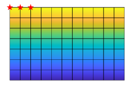
Figure 3: This figure illustrates how to choose control nodes on the grid graph $\mathcal{L}_{m,n}$ such that $(L(m,n),\bar{B})$ is controllable for $m\neq n$, where the control nodes are marked by red stars.

Generally speaking, it is difficult to give all the control node sets such that $(L(m,n),\bar{B})$ is controllable for given $m$ and $n$. However, for some special cases, we can solve this problem completely by using our results.

• For the case $\psi(m,n)=1$, Notarstefano and Parlangeli in Notarstefano and Parlangeli, (2013) gave all and only the combinations of control nodes for $(L(m,n),\bar{B})$ to be controllable, though they did not show under what conditions $\psi(m,n)=1$ holds. Our Corollary 2 gives the answer for this question. Thus, for the case $\psi(m,n)=1$, the problem of finding all the control node sets for the pair $(L(m,n),\bar{B})$ to be controllable is thoroughly solved.

• Another case where this problem can be solved thoroughly is $\mathbf{d}=1$, $2|m$, $3|n$ and $5\nmid m$ so that $\varphi(m,n)=\psi(m,n)=2$ (see Corollary 2 and Theorem 2), where $5\nmid m$ means that $5$ is not a factor of $m$. For this case, $L(m,n)$ has only one multiple eigenvalue whose multiplicity is 2. We can find all the control node combinations such that (29) holds by calculating the determinant of $2\times 2$ square matrices. Thus, all the control node sets such that $(L(m,n),\bar{B})$ is controllable can be obtained.

4.2 Controllability of system (12) on cylinder grid graphs

In Subsection 4.1, we investigate controllability of system (12) on grid graphs. In fact, the methods in the above subsection can also be extended to study controllability of system (12) on $m\times n$ cylinder grid graphs $\mathcal{C}_{m,n}$. The Laplacian matrix of $\mathcal{C}_{m,n}$ is denoted as $L_{\mathcal{C}}(m,n)$.

By Subsection 2.1 , we know that a cylinder grid graph $\mathcal{C}_{m,n}$ is the Cartesian product of a cycle graph $\mathcal{D}_{m}$ and a path graph $\mathcal{P}_{n}$. In order to provide properties of eigenvalues and eigenvectors of $L_{\mathcal{C}}(m,n)$, we introduce a lemma which gives the explicit expression of eigenvalues and eigenvectors of the Laplacian matrix $L_{\mathcal{D}}(m)$ of the cycle graph $\mathcal{D}_{m}$.

Lemma 7 (Godsil and Royle, (2001)).

The eigenvalues $\lambda^{(\mathcal{D})}_{1},\cdots,\lambda^{(\mathcal{D})}_{m}$ of $L_{\mathcal{D}}(m)$ are given by

$$\lambda^{(\mathcal{D})}_{\alpha}=2-2\cos{\frac{2\alpha\pi}{m}},\ \alpha=1,2,\cdots,m,$$ (32)

and the corresponding eigenvectors $\bar{v}_{\alpha}=[\bar{v}_{\alpha,1},\cdots,\bar{v}_{\alpha,m}]^{T}$ are given by

$$\bar{v}_{\alpha,j}=\mathbf{e}^{\mathbf{i}\frac{2\alpha j\pi}{m}},\ j=1,2,\cdots,m,$$

where $\mathbf{i}$ is the unit of imaginary number and $\mathbf{e}$ is the base of natural logarithm.

Based on the above lemma, we have the following results about eigenvalues and eigenvectors of the Laplacian matrix $L_{\mathcal{C}}(m,n)$.

Lemma 8.

The Laplacian matrix $L_{\mathcal{C}}(m,n)$ has the following $mn$ eigenvalues,

$$\hat{\lambda}_{\alpha\beta}=4-2(\cos{\frac{2\alpha\pi}{m}}+\cos{\frac{\beta\pi}{n}}),1\leq\alpha\leq m,0\leq\beta\leq n-1.$$ (33)

The eigenvector corresponding to $\hat{\lambda}_{\alpha\beta}$ is $\bar{v}_{\alpha}\otimes w_{\beta}$, where $\bar{v}_{\alpha}=[\bar{v}_{\alpha,1},\cdots,\bar{v}_{\alpha,m}]^{T}$ with $\bar{v}_{\alpha,k}=\mathbf{e}^{\mathbf{i}\frac{2\alpha k\pi}{m}}$ for $1\leq k\leq m$ and $w_{\beta}=[w_{\beta,1},\cdots,w_{\beta,n}]^{T}$ with $w_{\beta,l}$ defined in (15).

Parallel to Corollary 2, we have the following result for the largest multiplicity of eigenvalues of $L_{\mathcal{C}}(m,n)$ by using Lemma 6.

Corollary 3.

Let $\psi_{\mathcal{C}}(m,n)(m\geq 3,n\geq 2)$ denote the largest multiplicity of eigenvalues of $L_{\mathcal{C}}(m,n)$, and $\mathbf{d}_{\mathcal{C}}$ denote the greatest common divisor of $m$ and $2n$. We have

• for $\mathbf{d}_{\mathcal{C}}\geq 6$, $\psi_{\mathcal{C}}(m,n)=\mathbf{d}_{\mathcal{C}}-1$;

• for $\mathbf{d}_{\mathcal{C}}=5$,

  $$\psi_{\mathcal{C}}(m,n)=\begin{cases}6,&\mbox{if $(15|m,10|n)$;}\\ 4&\mbox{otherwise;}\end{cases}$$

• for $\mathbf{d}_{\mathcal{C}}=4$,

  $$\psi_{\mathcal{C}}(m,n)$$

  $$=\begin{cases}4,&\mbox{if ($10|m$, $3|n$) or ($12|m$, $5|n$) or ($6|m$, $2|n$);}\\ 3&\mbox{otherwise;}\end{cases}$$

• for $\mathbf{d}_{\mathcal{C}}=3$, $\psi_{\mathcal{C}}(m,n)=3$;

• for $\mathbf{d}_{\mathcal{C}}=2$,

  $$\psi_{\mathcal{C}}(m,n)$$

  $$=\begin{cases}4,&\mbox{if $(10|m,3|n)$ or $(12|m,5|n)$ or $(6|m,2|n)$;}\\ 3,&\mbox{otherwise if $(6|m,5|n)$ or $(4|m,3|n)$;}\\ 2,&\mbox{otherwise;}\end{cases}$$

• for $\mathbf{d}_{\mathcal{C}}=1$, $\psi_{\mathcal{C}}(m,n)=2$.

The proof of this corollary follows that of Corollary 2.

Based on Lemma 6, Lemma 8 and Corollary 3, we can establish the following theorem about the minimal number of control nodes such that $(L_{\mathcal{C}}(m,n),\bar{B})$ is controllable.

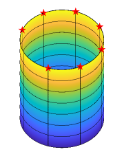
Figure 4: This figure illustrates how to choose control nodes on the cylinder grid graph $\mathcal{C}_{m,n}$ such that $(L_{\mathcal{C}}(m,n),\bar{B})$ is controllable, where the control nodes are marked by red stars.

Theorem 3.

Denote $\varphi_{\mathcal{C}}(m,n)$ as the minimal number of control nodes such that $(L_{\mathcal{C}}(m,n),\bar{B})$ is controllable, that is,

$$\varphi_{\mathcal{C}}(m,n)=\min\big{\{}\rho\in\mathbf{Z}^{+}|there\ exist\ i_{1},...,i_{\rho},1\leq$$

$$i_{1},...,i_{\rho}\leq mn,such\ that\ (L_{\mathcal{C}}(m,n),[e^{(mn)}_{i_{1}},\cdots,e^{(mn)}_{i_{\rho}}])\$$

$$is\ controllable\big{\}}.$$

Then we have $\varphi_{\mathcal{C}}(m,n)=\psi_{\mathcal{C}}(m,n)$.

Proof.

The control nodes to guarantee controllability of $(L_{\mathcal{C}}(m,n),\bar{B})$ can be chosen as $\psi_{\mathcal{C}}(m,n)$ consecutive nodes in the first row of the cylinder grid graph as illustrated in Fig. 4. It is clear that the corresponding control matrix is $\bar{B}=[e^{(m)}_{1},\cdots,e^{(m)}_{\psi_{\mathcal{C}}(m,n)}]\otimes e^{(n)}_{1}$. By following the proof line of Theorem 2, we can obtain the reuslts of the theorem. ∎

5 Concluding remarks

This paper investigates controllability of networked multiagent systems which are obtained by linearizing and spatial discretizing Turing’s model. We first establish the equivalence between controllability of the second-order linearized Turing’s model and the Laplace dynamic system under mild conditions on parameters of the model. Then, with the help of solutions of the trigonometric diophantine equation, we characterize multiplicities of eigenvalues of the Laplacian matrix of grid graphs and cylinder grid graphs. Based on this analysis, we give a complete characterization for the controllability problem of the linearized Turing’s model on these two graphs by not only providing minimal numbers of control nodes but also choosing corresponding control node sets to guarantee controllability of the system.

References

- Aguilar and Gharesifard, (2015) Aguilar, C. and Gharesifard, B. (2015). Graph controllability classes for the Laplacian leader-follower dynamics. IEEE Transactions on Automatic Control, 60(6):1611–1623.
- Bacciotti, (2019) Bacciotti, A. (2019). Stability and Control of Linear Systems. Springer International Publishing, Cham.
- Cao et al., (2013) Cao, M., Zhang, S., and Camlibel, M. (2013). A class of uncontrollable diffusively coupled multiagent systems with multichain topologies. IEEE Transactions on Automatic Control, 58(2):465–469.
- Chapman et al., (2014) Chapman, A., Nabi-Abdolyousefi, M., and Mesbahi, M. (2014). Controllability and observability of network-of-networks via Cartesian products. IEEE Transactions on Automatic Control, 59(10):2668–2679.
- Commault and Dion, (2013) Commault, C. and Dion, J.-M. (2013). Input addition and leader selection for the controllability of graph-based systems. Automatica, 49(11):3322–3328.
- Conway and Jones, (1976) Conway, J. and Jones, A. (1976). Trigonometric diophantine equations (on vanishing sums of roots of unity). Acta Arithmetica, 30:229–240.
- Gierer and Meinhardt, (1972) Gierer, A. and Meinhardt, H. (1972). A theory of biological pattern formation. Kybernetik, 12:30–39.
- Godsil, (2012) Godsil, C. (2012). Controllable subsets in graphs. Annals of Combinatorics, 16(4):733–744.
- Godsil and Royle, (2001) Godsil, C. and Royle, G. (2001). Algebraic Graph Theory. Springer New York, New York.
- Hao et al., (2018) Hao, Y., Duan, Z., and Chen, G. (2018). Further on the controllability of networked MIMO LTI systems. International Journal of Robust and Nonlinear Control, 28(5):1778–1788.
- (11) Hao, Y., Duan, Z., Chen, G., and Wu, F. (2019a). New controllability conditions for networked, identical LTI systems. IEEE Transactions on Automatic Control, 64(10):4223–4228.
- (12) Hao, Y., Wang, Q., Duan, Z., and Chen, G. (2019b). Controllability of Kronecker product networks. Automatica, 110:108597.
- Horn and Johnson, (2012) Horn, R. and Johnson, C. (2012). Matrix Analysis. Cambridge University Press, Cambridge, 2nd edition.
- Ji et al., (2012) Ji, Z., Lin, H., and Yu, H. (2012). Leaders in multi-agent controllability under consensus algorithm and tree topology. Systems Control Letters, 61(9):918–925.
- Ji and Yu, (2017) Ji, Z. and Yu, H. (2017). A new perspective to graphical characterization of multiagent controllability. IEEE Transactions on Cybernetics, 47(6):1471–1483.
- Maini et al., (2012) Maini, P., Woolley, T., Baker, R., Gaffney, E., and Lee, S. (2012). Turing’s model for biological pattern formation and the robustness problem. Interface focus, 2(4):487–496.
- Mousavi et al., (2021) Mousavi, S., Haeri, M., and Mesbahi, M. (2021). Laplacian dynamics on cographs: Controllability analysis through joins and unions. IEEE Transactions on Automatic Control, 66(3):1383–1390.
- Nabi-Abdolyousefi and Mesbahi, (2013) Nabi-Abdolyousefi, M. and Mesbahi, M. (2013). On the controllability properties of circulant networks. IEEE Transactions on Automatic Control, 58(12):3179–3184.
- Notarstefano and Parlangeli, (2013) Notarstefano, G. and Parlangeli, G. (2013). Controllability and observability of grid graphs via reduction and symmetries. IEEE Transactions on Automatic Control, 58(7):1719–1731.
- Olshevsky, (2014) Olshevsky, A. (2014). Minimal controllability problems. IEEE Transactions on Control of Network Systems, 1(3):249–258.
- Parlangeli and Notarstefano, (2012) Parlangeli, G. and Notarstefano, G. (2012). On the reachability and observability of path and cycle graphs. IEEE Transactions on Automatic Control, 57(3):743–748.
- Rahmani et al., (2009) Rahmani, A., Ji, M., Mesbahi, M., and Egerstedt, M. (2009). Controllability of multi-agent systems from a graph-theoretic perspective. SIAM Journal on Control and Optimization, 48(1):162–186.
- Raspopovic et al., (2014) Raspopovic, J., Marcon, L., Russo, L., and Sharpe, J. (2014). Digit patterning is controlled by a bmp-sox9-wnt turing network modulated by morphogen gradients. Science, 345(6196):566–570.
- She et al., (2020) She, B., Mehta, S., Ton, C., and Kan, Z. (2020). Controllability ensured leader group selection on signed multiagent networks. IEEE Transactions on Cybernetics, 50(1):222–232.
- She et al., (2021) She, B., Mehta, S. S., Doucette, E., Ton, C., and Kan, Z. (2021). Characterizing energy-related controllability of composite complex networks via graph product. IEEE Transactions on Automatic Control, 66(7):3205–3212.
- Sheth et al., (2012) Sheth, R., Marcon, L., Bastida, M., Junco, M., Quintana, L., Dahn, R., Kmita, M., Sharpe, J., and Ros, M. (2012). Hox genes regulate digit patterning by controlling the wavelength of a Turing-type mechanism. Science, 338(6113):1476–1480.
- Sick et al., (2006) Sick, S., Reinker, S., Timmer, J., and Schlake, T. (2006). WNT and DKK determine hair follicle spacing through a reaction-diffusion mechanism. Science, 314(5804):1447–1450.
- Sun et al., (2017) Sun, C., Hu, G., and Xie, L. (2017). Controllability of multiagent networks with antagonistic interactions. IEEE Transactions on Automatic Control, 62(10):5457–5462.
- Tanner, (2004) Tanner, H. (2004). On the controllability of nearest neighbor interconnections. In Proceedings of the 43rd IEEE Conference on Decision and Control, 3:2467-2472, Nassau, Bahamas.
- Trumpf and Trentelman, (2019) Trumpf, J. and Trentelman, H. (2019). Controllability and stabilizability of networks of linear systems. IEEE Transactions on Automatic Control, 64(8):3391–3398.
- Turing, (1952) Turing, A. (1952). The chemical basis of morphogenesis. Philosophical Transactions of the Royal Society of London. Series B, Biological Sciences, 237(641):37–72.
- Wang et al., (2016) Wang, L., Chen, G., Wang, X., and Tang, W. (2016). Controllability of networked MIMO systems. Automatica, 69:405–409.
- Wlodarski, (1969) Wlodarski, L. (1969). On the equation . Annales Universitatis Scientarium Budapestinensis de Rolando Eötvös Nominatae Sectio Mathematica, 12:147–155.
- Yazıcıoğlu et al., (2016) Yazıcıoğlu, A., Abbas, W., and Egerstedt, M. (2016). Graph distances and controllability of networks. IEEE Transactions on Automatic Control, 61(12):4125–4130.
- Yuan et al., (2013) Yuan, Z., Zhao, C., Di, Z., Wang, W., and Lai, Y. (2013). Exact controllability of complex networks. Nature communications, 4:2447.
- Yueh, (2005) Yueh, W. (2005). Eigenvalues of several tridiagonal matrices. Applied Mathematics E-Notes, 5:66–74.
- Zhang and Zhou, (2017) Zhang, Y. and Zhou, T. (2017). Controllability analysis for a networked dynamic system with autonomous subsystems. IEEE Transactions on Automatic Control, 62(7):3408–3415.