On Forecast Stability

Abstract

Forecasts are typically not produced in a vacuum but in a business context, where forecasts are generated on a regular basis and interact with each other. For decisions, it may be important that forecasts do not change arbitrarily, and are stable in some sense. However, this area has received only limited attention in the forecasting literature. In this paper, we explore two types of forecast stability that we call vertical stability and horizontal stability. The existing works in the literature are only applicable to certain base models and extending these frameworks to be compatible with any base model is not straightforward. Furthermore, these frameworks can only stabilise the forecasts vertically. To fill this gap, we propose a simple linear-interpolation-based approach that is applicable to stabilise the forecasts provided by any base model vertically and horizontally. The approach can produce both accurate and stable forecasts. Using N-BEATS, Pooled Regression and LightGBM as the base models, in our evaluation on four publicly available datasets, the proposed framework is able to achieve significantly higher stability and/or accuracy compared to a set of benchmarks including a state-of-the-art forecast stabilisation method across three error metrics and six stability metrics.

1 Introduction

In many business applications, forecasts are produced on a regular basis and if the forecasts are volatile that can have negative consequences for subsequent decision-making steps. Thus, stability of the forecasts of some sort is often a desirable property. However, stability can be understood in different ways, e.g., it can mean that forecasts performed on different (origin) days for the same target day should not differ too much, or it can mean that forecasts within an output window should be stable/smooth in some way. It can also simply mean an ensembling/forecast combination step to “stabilize” the output of low-bias high-variance forecasting methods, such as neural networks. Finally, it can mean any combination of those.

The first mentioned type of stability is sometimes referred to as rolling origin forecast stability [23] in the literature. In real-world applications such as supply chain planning, the forecasting models are retrained when new observations become available, and thus, the forecast corresponding with a particular horizon can be produced multiple times considering different origins. If the forecasts corresponding with the same target made at different origins are unstable, then the decisions that are made based on the forecasts made at a previous origin are required to be significantly changed based on the forecasts made at a later origin. This leads to revisions of supply chain plans and can incur significant losses for the businesses [14, 25]. Thus, obtaining stable forecasts is oftentimes important for correct decision-making. In a recent very interesting paper, Van Belle et al. [26] propose an extension to the N-BEATS framework [19] to stabilise its forecasts in this rolling origin sense. Those authors modify the loss function of the original N-BEATS implementation to optimise both forecast accuracy and stability. The main limitation of that work that we observe is that, by the approach of using a modified loss function, the method needs to forecast for all origins to stabilise over, which does not coincede with the typical use case, where forecasts for older origins have already been produced and communicated to stakeholders, and therewith cannot be changed. Furthermore, the approach is not model-agnostic, as it may be difficult to implement for certain model classes; the original paper focuses on an implementation in the N-BEATS model. Moreover, the approach is only applicable to stabilise forecasts in the rolling origin manner.

Making the forecast stable in the sense of producing a smooth forecast over an output window can be important, e.g., in supply chain planning to reduce the bullwhip effect [13] which refers to a phenomenon of demand variation amplification in a supply chain consisting of a large number of parties including manufacturers, wholesalers, suppliers and customers. The unstable forecasts corresponding with one party in a supply chain may lead to higher fluctuations in demand information for other parties incurring significant costs. Thus, the bullwhip effect is a common high-risk phenomenon in the supply chain domain and obtaining stable forecasts over the full horizon is important to reduce this effect.

Ensembling can be identified as another approach to mitigate forecast instability. In the forecasting space, ensembling is also known as forecast combination [2, 24]. Ensembled models aggregate the predictions provided by multiple models to obtain final predictions. Ensembling can reduce model variance and model bias [22, 3] and thus, it provides stable forecasts compared to the individual forecasting models [12, 27]. Forecast combinations are also used to stabilise forecasts in the macroeconomic forecasting domain [1]. The winning method of the M5 forecasting competition [8] also uses an ensembling approach where it considers the simple average of the forecasts obtained using direct and recursive methods as the final forecasts. The direct method directly produces the forecasts corresponding with a particular target time point from a prior forecasting origin. The recursive method iteratively produces the forecasts one-by-one starting from a particular forecast origin. Thus, the final forecast produced by this method corresponding with a particular target time point is an ensemble of the forecasts obtained for the same target time point from different forecast origins. In that sense, the forecasts are stable and as the method won the competition, the forecasts are highly accurate as well. However, the authors have not explored the stability of the forecasts provided by the method.

In this paper, we first take a systematic approach and introduce a categorisation for different types of forecast stability. There is a perceived trade-off between accuracy and stability. However, the findings of Van Belle et al. [26] and In and Jung [8] lead us to believe that sometimes it is possible to obtain forecasts that are both accurate and stable. Motivated by this, we then propose a simple and generic yet powerful model-agnostic linear interpolation based approach to stabilise the forecasts in all different forecast stability categories. In the experiments, we are able to show that for many datasets, our approach produces both significantly more accurate and stable forecasts compared to the base models whereas on the other datasets, it produces much more stable forecasts with quite modest accuracy losses. All implementations of this study are publicly available at: https://tinyurl.com/ycxt95rm.

The remainder of this paper is organized as follows. Section 2 introduces our stability categorisation and our proposed linear interpolation approach in detail. Section 3 discusses the experimental framework, including the datasets, error metrics, base models and benchmarks. Section 4 presents an analysis of the results. Section 5 concludes the paper and discusses possible future research.

2 Methodology

In this section, we first explain the proposed stability categorisation, and then introduce the proposed model-agnostic approach that can be used to stabilise forecasts.

2.1 Categorisation of Types of Forecast Stability

We identify four different types of stability, depending on the same or different forecast origins and targets of the methods, as shown in Figure 1. In particular, we may want to achieve stability between forecasts that have been produced:

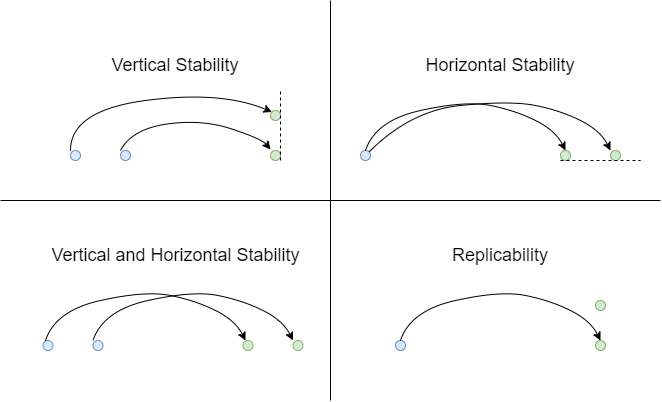
Figure 1: A visualisation of four different forecast stability types: vertical stability, horizontal stability, vertical and horizontal stability, and replicability. The blue and green dots respectively represent the origin that the forecasts are made and the target.

1. from the same origin and for the same target. This is effectively ensembling or a forecast combination approach. We call this replicability in the following.

2. from different origins for the same target. We’ll call this vertical stability in the following, as the forecasting target is at the same time stamp, and therewith the desired stability is vertical on the time axis.

3. from the same origin for different targets. We’ll call this horizontal stability, as the desired stability is horizontal with respect to the time axis of the forecast targets.

4. from different origins for different targets. This form of stability is a mix of both horizontal and vertical stability.

As ensembling has been covered extensively elsewhere and we deem it not the main focus of our paper, we discuss in the following vertical and horizontal stability in more detail.

Vertical Stability

In real-world applications, often the forecasts are obtained in a rolling origin fashion. Thus, the forecasts corresponding with a particular target time point are obtained multiple times considering different forecast origins as shown in Figure 2. Let us assume a time series with 10 data points, T1-T10. A forecasting model is trained with the training data and 6-step ahead forecasts are obtained, H1-H6, with T10 as the origin. The number of forecasts made at a given origin, i.e., the forecasting horizon or forecasting window, is 6 in this example.

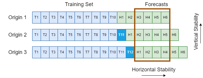
Figure 2: Visualisation of the concepts of vertical and horizontal stability types.

In real-world applications, new data points become available as time passes. Thus, when the next data point, T11, becomes available, it is added to the training set. Again, 6-step ahead forecasts are made considering T11 as the new, second, origin. When T12 becomes available, it is also added to the training set, and considering T12 as the third origin, 6-step ahead forecasts are again made. We can see from the figure that the forecast output windows overlap, so that forecasts made at different origins are corresponding with the same target time point. For example, consider the forecasts provided by adjacent forecast origins. Here, the forecasts H2-H6 at origin 1 and H1-H5 at origin 2, and H2-H6 of origin 2 and H1-H5 of origin 3 are corresponding with the same time periods. Non-adjacent forecast origins also provide forecasts corresponding with the same time period, e.g., forecasts H3-H6 at origin 1, H2-H5 at origin 2 and H1-H4 at origin 3 (brown box). Thus, depending on the step size in which the origin is moved and the size of the forecasting window, not only two forecasts will be made for the same target value, but potentially many more.

To achieve vertical stability, our goal is that forecasts produced at multiple origins for the same time period are close. Otherwise, the decisions (e.g., the number of products that should be ordered for the next 6 weeks) made based on the forecasts provided at a previous origin may require to be significantly changed based on the forecasts provided at a later origin, potentially incurring significant order adjustment costs. Thus, the forecasts corresponding with the same time period made at different origins should be vertically stable for proper decision-making.

Only the last forecasts are produced for time points for which no previous forecasts already exist. As such, these new forecasts can be produced purely in a way to maximise accuracy. All other forecasts are merely updates of already existing forecasts. As we assume that the previous forecasts have already been communicated to stakeholders, they cannot be changed anymore, and the new forecasts need to be “anchored” at the old forecasts, to achieve vertical stability. Now, assuming that newer forecasts will be more accurate, as they can incorporate additional, new data points not available before, predicting with a shorter horizon, it is clear that there is a trade-off between accuracy and stability.

Horizontal Stability

The concept of horizontal stability is for forecasts produced from the same origin. As shown in Figure 2, to achieve horizontal stability, the forecasts H1-H6 that are made at the same origin are required to be close to each other. Thus, the adjacent forecasts: H1 and H2, H2 and H3, H3 and H4, H4 and H5, and H5 and H6, need to be close. This eventually tries to make the forecasts smooth throughout the forecast horizon.

Horizontally stable forecasts are useful in some real-world applications, to counter the so-called bullwhip effect in supply chains. For example, consider a supply chain that contains a manufacturer, a supplier, and customers. When the product sales at the customer end are predicted to be increased, then more products are required to be ordered from the supplier. In general, the supplier orders products from the manufacturer with a buffer, and thus, they will order more products from the manufacturer to fulfill the customer demand. The manufacturer also produces goods with a buffer and thus, they will produce even more goods. Thus, the small fluctuations at the customer end may result in larger fluctuations at the manufacturer end. The horizontally stable forecasts reduce the fluctuations in the forecasts from the consumer end and thus, they reduce the bullwhip effect.

Note that horizontal stability is not always desirable. For example, when there are known future promotions in retail we expect the forecasts to change sharply and not be smooth. Also, other highly predictable patterns, namely trend and seasonality, can be present. In such situations, we could develop horizontally stable forecasts that are seasonally smoothed, so that they show smooth seasonalities and trends, or we could introduce smoothing weights that change based on the amount of smoothing desired. Though it is a simplification, as even many of the datasets in our experiments have trends and seasonality, in this paper we focus on the most basic stationary case as an illustration of the general process, without further considerations of, e.g., trend and seasonality handling.

2.2 Proposed Framework

The main prior work that we are aware of to tackle (vertical) stability is the work of Van Belle et al. [26], where those authors build a model that produces forecasts directly for two origins, and couples them in the loss function to be vertically stable. The main drawback of using custom loss functions to achieve stability is that this approach does not adequately capture the normal use case. In a normal use case, forecasts from a previous origin will have already been produced and communicated to stakeholders, so they cannot be changed anymore. They are an input to the algorithm, not an output. Thus, the approach of Van Belle et al. [26] is somewhat ineffective in the sense that all forecasts are produced twice, with one version being discarded. More importantly, the stabilisation is performed not against the actual prior forecasts but against newly built and adapted “prior” forecasts. This holds the implicit assumption that the prior forecasts have been produced with a similar model/methodology and resemble similar properties as the newly produced “prior” forecasts. This assumption may be limiting in many applications. Furthermore, the approach is limited to stabilise over two forecasts, while in practice, as shown in Section 2.1, usually more forecasts need to be stabilised over.

Due to these considerations, we propose in our work not to use the approach of a custom loss function, but to take a step back and use a simpler approach, namely linear interpolation. This approach is straightforward and has been implicitly used in some forms in the literature. Van Belle et al. [26] present a comparison method using the N-BEATS model, namely N-BEATS origin ensemble. As the final forecast of a particular target time point, this method produces the simple average of the forecasts made at prior origins and the current origin corresponding with that target time point. In contrast, we apply linear interpolation for the forecasts made at adjacent forecast origins, separately, considering both simple and weighted averaging. The winning approach of the M5 forecasting competition [8] also implicitly considers the simple average of the forecasts obtained using different forecast origins as the final forecasts, however, the authors have not explored the stability of the forecasts produced by their method.

This is the first study to present a systematic analysis showing the usage of linear interpolation to stabilise forecasts with state-of-the-art machine learning tools and datasets. It has the advantage that it can be used in a model-agnostic way, even for situations where different methodologies are used for different forecast iterations (i.e., different origins), it is fast to compute, and it allows in a very straightforward way to control the trade-off between accuracy and stability, without the need to recompute the base forecasts.

2.2.1 Linear Interpolation for Vertical Stability

As shown in Figure 2, consider an example situation where the forecasts are required to be vertically stabilised across 3 consecutive origins where 6-step ahead forecasts are made at each origin. Thus, in this case, the forecast horizon (h) is 6. The forecasts, H2-H6 at a given origin and the forecasts, H1-H5 at the next origin are corresponding with the same time period. Thus, those forecasts should be close to each other to achieve vertical stability.

Note that the forecasts made at the first origin of each series cannot be stabilised as those are the very first forecasts obtained from the series. The last forecast made at each origin also cannot be stabilised as those are the very first forecasts corresponding with a particular time point. Thus, for each series, the forecasts are required to be stabilised from the second origin onwards except the last forecasts.

The forecasts made at a given origin can be stabilised by linearly combining them with the forecasts made at the previous origin in a pairwise manner or linearly combining them with the forecasts made at all prior origins together. For simplicity, in this work, the forecasts made at adjacent origins are linearly combined to make them stable.

Thus, the stable forecasts at the second origin are obtained as a linear combination of the original forecasts made at the second origin and the corresponding forecasts made at the first origin as shown in Equation 1. Here, $SF_{O_{2}H_{j}}$ is the stable forecast of the $j^{th}$ horizon at origin 2, $F_{O_{2}H_{j}}$ is the original forecast of the $j^{th}$ horizon made at origin 2, $F_{O_{1}H_{j+1}}$ is the corresponding original forecast made at origin 1, and $w\_s$ is the weight of the corresponding forecast made at origin 1, where $1\leq j<h$ and $0\leq w\_s\leq 1$.

$$SF_{O_{2}H_{j}}=(w\_s)F_{O_{1}H_{j+1}}+(1-w\_s)F_{O_{2}H_{j}}$$ (1)

From the third origin onwards, linear interpolation can be performed in two ways to stabilise forecasts. We name these two methods as partial interpolation and full interpolation. Equations 2 and 3 show the formulas of partial and full interpolation, respectively, where $SF_{O_{i}H_{j}}$ is the stable forecast of the $j^{th}$ horizon at $i^{th}$ origin, $F_{O_{i}H_{j}}$ is the original forecast of the $j^{th}$ horizon made at $i^{th}$ origin and $w\_s$ is the weight of the corresponding forecast made at $(i-1)^{th}$ origin, where $i>2$ and $1\leq j<h$ and $0\leq w\_s\leq 1$.

$$SF_{O_{i}H_{j}}=(w\_s)F_{O_{i-1}H_{j+1}}+(1-w\_s)F_{O_{i}H_{j}}$$ (2)

$$SF_{O_{i}H_{j}}=(w\_s)SF_{O_{i-1}H_{j+1}}+(1-w\_s)F_{O_{i}H_{j}}$$ (3)

As shown in Equations 2 and 3, the difference between partial and full interpolation methods is that to obtain stable forecasts at the current origin, partial interpolation considers the corresponding original forecasts at the previous origin whereas full interpolation considers the corresponding interpolated stable forecasts at the previous origin. Thus, partial interpolation considers the forecasts made at adjacent forecast origins and combines the forecasts in a pairwise manner. Even though full interpolation combines the forecasts corresponding with adjacent forecast origins, it also takes the forecasts made at all prior origins into account as the prior interpolated stable forecasts are used during the interpolation. In that sense, full interpolation combines the forecasts in a chained manner where higher weights are given for the forecasts made at closer origins. In general, full interpolation is closer to a practical use case as the forecasts at a given origin should be stable with respect to the forecasts corresponding with the prior origin, not the original forecasts, but the stable forecasts which are already communicated to the stakeholders.

2.2.2 Linear Interpolation for Horizontal Stability

The concept of horizontal stability considers the adjacent forecasts made at a given origin. For the example shown in Figure 2, it requires the adjacent forecasts such as H1 and H2, H2 and H3, H3 and H4, H4 and H5, and H5 and H6 of any origin to be closer.

It is not possible to horizontally stabilise the forecasts corresponding with the first horizon, H1. Thus, for each series and origin, the forecasts are required to be stabilised from H2 onwards.

The stable forecasts corresponding with H2 are obtained as a linear combination of the original H2 and H1 forecasts as shown in Equation 4. Here, $SF_{H_{2}}$ is the stable H2 forecast, $F_{H_{2}}$ is the original H2 forecast, $F_{H_{1}}$ is the original H1 forecast, and $w\_s$ is the weight given for H1 forecast, where $0\leq w\_s\leq 1$.

$$SF_{H_{2}}=(w\_s)F_{H_{1}}+(1-w\_s)F_{H_{2}}$$ (4)

From H3 onwards, either partial or full interpolation can be performed to stabilise forecasts. Equations 5 and 6 respectively show the formulas of partial and full interpolation that are used to make the forecasts horizontally stable, where $SF_{H_{j}}$ is the stable forecast of the $j^{th}$ horizon, $F_{H_{j}}$ is the original forecast of the $j^{th}$ horizon and $w\_s$ is the weight given for the forecast of the $(j-1)^{th}$ horizon, where $1<j\leq h$ and $0\leq w\_s\leq 1$.

$$SF_{H_{j}}=(w\_s)F_{H_{j-1}}+(1-w\_s)F_{H_{j}}$$ (5)

$$SF_{H_{j}}=(w\_s)SF_{H_{j-1}}+(1-w\_s)F_{H_{j}}$$ (6)

Similar to the vertical stability, here also the difference between partial and full interpolation methods is that to obtain stable forecasts for the current horizon, partial interpolation considers the corresponding original forecasts from the previous horizon whereas full interpolation considers the interpolated stable forecasts from the previous horizon.

For our experiments, we analyse the effect of both partial and full interpolation methods to gain vertical and horizontal stability with different weights for $w\_s$, namely 0.2, 0.4, 0.5, 0.6, 0.8, and 1.

3 Experimental Framework

In this section, we discuss the datasets, error metrics, base models, and benchmarks used in our experiments.

3.1 Datasets

We use four publicly available datasets to evaluate the performance of our proposed framework. Table 1 provides a summary of the datasets. A brief overview of the datasets is as follows.

• M4 Monthly Dataset: The monthly dataset of the M4 forecasting competition [16].

• M3 Monthly Dataset: The monthly dataset of the M3 forecasting competition [15].

• Favorita Dataset [9]: The first 1000 time series from the Corporación Favorita Grocery Sales forecasting competition. Each series shows daily unit sales of a particular item sold at a Favorita store. The missing observations of this dataset are replaced by zeros.

• M5 Items Dataset: An aggregated version of the M5 forecasting competition dataset [17] where the daily unit sales of individual items have been aggregated across Walmart stores in different states.

Dataset	No. of	No. of	Forecast	Min.	Max.
	Series	Origins	Horizon	Length	Length
M4	48000	13	6	60	2812
M3	1428	13	6	66	144
Favorita	1000	11	6	1684	1684
M5	3049	13	16	1969	1969

Table 1: Summary of the used Datasets

The major reason for using the M3 monthly and M4 monthly datasets is to compare the performance of the proposed approach against the Stable N-BEATS approach [26]. Those authors have used all the sub-datasets of the M3 and M4 forecasting competitions for their experiments and for a fair comparison, we have used the monthly versions of both datasets which are the corresponding largest sub-datasets in terms of the number of time series. Furthermore, to add some diversity into the pool of datasets, we consider the Favorita and M5 items datasets which are real-world retail datasets where our proposed approach is highly useful in practice.

3.2 Error Metrics

We use three error measures to evaluate the forecast accuracy and six error measures to evaluate the forecast stability. These error measures are explained in the following.

3.2.1 Accuracy Measures

The accuracy of the forecasts is evaluated using three error measures that are common in the forecasting research space: symmetric Mean Absolute Percentage Error (sMAPE), Mean Absolute Error [MAE, 21] and Root Mean Squared Error (RMSE), which are respectively defined in Equations 7, 8 and 9. For a given dataset, the forecast accuracy is evaluated across series with multiple forecast origins. Thus, the error measures are defined across one to $h$-step ahead forecasts resulting from a specific forecasting origin $t$, where $h$ is the forecast horizon, $y_{t+i}$ is the actual series value at time $t+i$ and $\hat{y}_{t+i|t}$ is the forecast corresponding with time $t+i$ made at time $t$.

$$\textit{sMAPE}=\frac{200\%}{h}\sum_{i=1}^{h}\frac{|y_{t+i}-\hat{y}_{t+i|t}|}{|y_{t+i}|+|\hat{y}_{t+i|t}|}$$ (7)

$$\textit{MAE}=\frac{\sum_{i=1}^{h}{|y_{t+i}-\hat{y}_{t+i|t}|}}{h}$$ (8)

$$\textit{RMSE}=\sqrt{\frac{\sum_{i=1}^{h}{|y_{t+i}-\hat{y}_{t+i|t}|}^{2}}{h}}$$ (9)

To measure the performance of the models on a dataset, we further calculate the mean values of sMAPE, MAE, and RMSE across multiple forecast origins in all series. Thus, the accuracy of each model is finally evaluated using three error metrics: mean sMAPE, mean MAE and mean RMSE, across a dataset.

3.2.2 Stability Measures

The stability of the forecasts is evaluated using six error measures that are following the stability metrics introduced by Van Belle et al. [26]. The definitions of the error measures are changed for vertical and horizontal stability types, which are explained in the following. To measure vertical stability, Van Belle et al. [26] propose symmetric Mean Absolute Percentage Change (sMAPC), which is defined in Equation 10.

$$\textit{sMAPC}(V)=\frac{200\%}{(h-1)}\sum_{i=1}^{h-1}\frac{|\hat{y}_{t+i|t}-\hat{y}_{t+i|t-1}|}{|\hat{y}_{t+i|t}|+|\hat{y}_{t+i|t-1}|}$$ (10)

Here, sMAPC measures the change of one to $h$-step ahead forecasts corresponding with two adjacent forecast origins, $t$ and $t-1$. Thus, it provides a measurement of up to which extent the forecasts generated at origin $t$ are stable compared to the forecasts generated at origin $t-1$ for the same time period. In line with the definition of sMAPC, we also define two other stability measures, Mean Absolute Change (MAC) and Root Mean Squared Change (RMSC), which compare the change between the forecasts generated at two adjacent forecast origins for the same time period. The MAC and RMSC are defined in Equations 11 and 12, respectively.

$$\textit{MAC}(V)=\frac{\sum_{i=1}^{h-1}{|\hat{y}_{t+i|t}-\hat{y}_{t+i|t-1}|}}{h-1}$$ (11)

$$\textit{RMSC}(V)=\sqrt{\frac{\sum_{i=1}^{h-1}{|\hat{y}_{t+i|t}-\hat{y}_{t+i|t-1}|}^{2}}{h-1}}$$ (12)

We also measure the vertical forecast stability in terms of the change between the forecasts generated at origin $t$ and the very first set of forecasts generated for the same time period at a previous origin. We name sMAPC, MAC, and RMSC calculated in this way as sMAPC_I, MAC_I and RMSC_I. When calculating sMAPC_I, MAC_I and RMSC_I for vertical stability, the term $\hat{y}_{t+i|t-1}$ in Equations 10, 11 and 12 is replaced with the very first forecast corresponding with time $t+i$ generated at a previous origin.

The horizontal stability measures the change of forecasts generated at the same origin. Thus, to measure horizontal forecast stability, the definitions of sMAPC, MAC and RMSC are respectively changed as shown in Equations 13, 14 and 15.

$$\textit{sMAPC}(H)=\frac{200\%}{(h-1)}\sum_{i=2}^{h}\frac{|\hat{y}_{t+i|t}-\hat{y}_{t+i-1|t}|}{|\hat{y}_{t+i|t}|+|\hat{y}_{t+i-1|t}|}$$ (13)

$$\textit{MAC}(H)=\frac{\sum_{i=2}^{h}{|\hat{y}_{t+i|t}-\hat{y}_{t+i-1|t}|}}{h-1}$$ (14)

$$\textit{RMSC}(H)=\sqrt{\frac{\sum_{i=2}^{h}{|\hat{y}_{t+i|t}-\hat{y}_{t+i-1|t}|}^{2}}{h-1}}$$ (15)

The sMAPC_I, MAC_I, and RMSC_I are also redefined for horizontal stability. For a given origin $t$, these stability measures calculate the change between the forecasts from time $t+2$ onwards with the first forecast at time $t+1$. Thus, to calculate sMAPC_I, MAC_I, and RMSC_I for horizontal stability, the term $\hat{y}_{t+i-1|t}$ in Equations 13, 14 and 15 is replaced with $\hat{y}_{t+1|t}$.

For a given dataset, all stability measures are calculated per each series and origin. Thus, to measure the forecast stability of the models on a dataset, the mean values of sMAPC, MAC, RMSC, sMAPC_I, MAC_I, and RMSC_I are calculated across multiple forecast origins in all series. Thus, the vertical stability and horizontal stability of each model are finally evaluated using six error metrics: mean sMAPC, mean MAC, mean RMSC, mean sMAPC_I, mean MAC_I, and mean RMSC_I, across a dataset. For the remainder of the paper, the names of the error metrics are not accompanied by the term, mean.

3.3 Experimental Base Models and Benchmarks

Our proposed framework is model-agnostic and it is applicable to stabilise the forecasts obtained from any forecasting model. However, for the experiments, we use three base models: N-BEATS [19], Pooled Regression [PR, 5, 18] and LightGBM [10] to evaluate the performance of the proposed framework. The method proposed by Van Belle et al. [26] is applicable to stabilise the forecasts of N-BEATS and thus, we use N-BEATS as a base model for the experiments. LightGBM is a highly efficient gradient-boosted tree that recently obtained massive popularity in the forecasting domain after contributing to most of the top solutions of the M5 forecasting competition [17]. To further add some diversity into the pool of base models, we consider PR as a base model which is a globally trained linear model.

We use the N-BEATS implementation by Van Belle et al. [26] for the experiments. The original N-BEATS model is executed by setting the parameter $\lambda$ in the implementation to zero. The Stable N-BEATS model is also executed as a benchmark by setting $\lambda$ to the corresponding optimal values provided in Van Belle et al. [26]. The remaining parameters of the N-BEATS model are also set to the parameters given in Van Belle et al. [26]. As the performance of the N-BEATS implementation highly depends on the parameters, the N-BEATS models are only executed across the M3 monthly and M4 monthly datasets where the optimal values of all parameters are available in Van Belle et al. [26].

The R packages glmnet [4] and lightgbm [11] are respectively used to implement PR and LightGBM models. The LightGBM model is executed with the default hyperparameter values except for learning rate, minimum instances in a leaf node, and the number of estimators where the values of these parameters are respectively set to 0.075, 100, and 100. The PR model does not require parameters. The LightGBM and PR models are executed across all datasets.

The number of lagged values used in PR and LightGBM are determined using a heuristic suggested by Hewamalage et al. [7]. In particular, the number of lags is considered as $seasonality\times 1.25$ of the dataset. Thus, we consider 9 and 15 lags for daily and monthly datasets, respectively.

The original N-BEATS, Stable N-BEATS, PR, and LightGBM models are also considered as the main benchmarks of this study.

3.4 Statistical Tests of the Results

We also perform pairwise tests for statistical significance using a Wilcoxon test [20] considering an initial significance level of $\alpha=0.05$. A Bonferroni correction is applied for $\alpha$ by dividing it with the number of comparisons made (for details, see Section 4.3).

4 Results and Discussion

This section explains the results of vertical and horizontal stability experiments and later provides more insights regarding the proposed models. The accuracy results are reported in terms of sMAPE and stability results are reported in terms of sMAPC and sMAPC_I. The Online Appendix contains the results of the other two error metrics: MAE and RMSE, and four stability metrics: MAC, MAC_I, RMSC and RMSC_I, and they are in agreement with the conclusions we draw by analysing sMAPE, sMAPC and sMAPC_I.

In the results tables, the terms PI and FI, respectively, denote the partial and full interpolation experiments. The numerical values next to the terms PI and FI show the corresponding w_s values considered during interpolation.

4.1 Results of Vertical Stability Experiments

Table 2 shows the results of vertical stability experiments across all experimental datasets for sMAPE, sMAPC and sMAPC_I. The experiments with the three base models: N-BEATS, PR, and LightGBM are separately grouped. The sub-experiments related to each base model are further divided into three groups. The first sub-group contains the benchmarks, the base models which do not use any stabilisation techniques. For N-BEATS models, the first sub-group also contains the Stable N-BEATS approach. The second and third sub-groups, respectively, show the partial and full interpolation experiments performed with the corresponding base model forecasts. The results of the best performing variants in each sub-group are italicized, and the overall best performing variants corresponding with a particular base model across the datasets are highlighted in boldface.

Table 2: sMAPE, sMAPC and sMAPC_I results of vertical stability experiments across all datasets. The best performing variants in each group are italicized and the overall best performing variants are highlighted in boldface. The * symbols represent the results that are significantly accurate or stable than the corresponding base models results across Favorita and M5 datasets.

	sMAPE				sMAPC				sMAPC_I
	M4	M3	Favorita	M5	M4	M3	Favorita	M5	M4	M3	Favorita	M5
N-BEATS
Base	9.296	11.485	-	-	4.717	3.932	-	-	6.468	5.786	-	-
Stable	9.279	11.390	-	-	3.336	2.820	-	-	5.270	4.705	-	-
PI_0.2	9.265	11.461	-	-	3.745	3.181	-	-	5.886	5.288	-	-
PI_0.4	9.324	11.484	-	-	3.050	2.649	-	-	5.386	4.850	-	-
PI_0.5	9.384	11.511	-	-	2.865	2.508	-	-	5.169	4.657	-	-
PI_0.6	9.464	11.553	-	-	2.808	2.451	-	-	4.976	4.485	-	-
PI_0.8	9.677	11.673	-	-	2.998	2.569	-	-	4.665	4.202	-	-
PI_1	9.956	11.831	-	-	3.450	2.889	-	-	4.462	4.000	-	-
FI_0.2	9.261	11.454	-	-	3.732	3.158	-	-	5.806	5.212	-	-
FI_0.4	9.318	11.458	-	-	2.851	2.444	-	-	4.991	4.483	-	-
FI_0.5	9.390	11.478	-	-	2.429	2.095	-	-	4.489	4.029	-	-
FI_0.6	9.502	11.518	-	-	2.008	1.743	-	-	3.897	3.492	-	-
FI_0.8	9.919	11.703	-	-	1.119	0.977	-	-	2.339	2.082	-	-
FI_1	10.806	12.219	-	-	0.000	0.000	-	-	0.000	0.000	-	-
PR
Base	10.632	12.622	103.351	54.964	3.245	3.518	29.190	17.559	5.282	4.896	36.772	26.876
PI_0.2	10.713	12.638	103.255	54.579	2.743	2.880	24.303	13.857	4.817	4.407	33.580	25.222
PI_0.4	10.822	12.680	$103.173^{*}$	54.392	2.350	2.385	$20.319^{*}$	11.260	4.390	3.971	$30.665^{*}$	23.894
PI_0.5	10.886	12.712	103.196	54.374	2.221	2.222	19.011	10.650	4.192	3.777	29.261	23.366
PI_0.6	10.956	12.751	103.269	54.406	2.142	2.132	18.160	10.565	4.007	3.604	27.930	22.935
PI_0.8	11.116	12.851	103.566	54.629	2.118	2.154	17.694	11.810	3.679	3.317	25.568	22.392
PI_1	11.302	12.981	104.084	55.087	2.244	2.388	18.739	14.375	3.418	3.128	23.677	22.273
FI_0.2	10.720	12.638	103.627	54.532	2.715	2.858	24.670	13.856	4.748	4.341	33.216	24.994
FI_0.4	10.860	12.685	103.530	54.162	2.177	2.217	19.386	10.504	4.064	3.661	28.954	22.720
FI_0.5	10.957	12.726	103.563	53.987	1.893	1.894	16.809	8.925	3.640	3.253	26.342	21.269
FI_0.6	11.080	12.783	103.673	53.812	1.594	1.565	13.911	7.361	3.144	2.786	23.174	19.446
FI_0.8	11.448	12.972	104.248	$53.556^{*}$	0.909	0.856	8.077	$4.213^{*}$	1.860	1.618	14.923	$13.662^{*}$
FI_1	12.103	13.333	105.775	54.936	0.000	0.000	0.000	0.000	0.000	0.000	0.000	0.000
LightGBM
Base	11.125	12.653	101.341	52.207	3.566	3.478	13.216	9.992	5.450	4.887	18.787	17.961
PI_0.2	11.211	12.680	101.229	52.100	2.950	2.812	10.796	8.108	4.939	4.412	16.703	16.996
PI_0.4	11.332	12.738	101.171	52.081	2.466	2.304	8.846	6.792	4.479	3.996	14.821	16.204
PI_0.5	11.405	12.779	101.155	52.092	2.307	2.146	8.146	6.445	4.270	3.813	13.963	15.862
PI_0.6	11.487	12.827	101.149	52.116	2.223	2.072	7.686	6.466	4.077	3.648	13.163	15.554
PI_0.8	11.673	12.944	101.164	52.209	2.237	2.146	7.359	7.063	3.744	3.375	11.764	15.057
PI_1	11.889	13.089	101.222	52.398	2.440	2.417	7.697	8.259	3.496	3.190	10.659	14.796
FI_0.2	11.221	12.683	101.214	52.079	2.929	2.798	10.701	8.029	4.868	4.349	16.457	16.826
FI_0.4	11.386	12.757	101.120	51.988	2.310	2.165	8.257	6.264	4.144	3.693	13.698	15.369
FI_0.5	11.503	12.815	101.086	51.946	1.993	1.852	7.025	5.398	3.701	3.297	12.087	14.393
FI_0.6	11.652	12.892	$101.067^{*}$	51.907	1.663	1.533	$5.768^{*}$	4.523	3.187	2.838	$10.274^{*}$	13.138
FI_0.8	12.087	13.136	101.107	$51.888^{*}$	0.929	0.845	3.095	$2.636^{*}$	1.868	1.665	5.861	$9.062^{*}$
FI_1	12.827	13.610	101.323	52.690	0.000	0.000	0.000	0.000	0.000	0.000	0.000	0.000

In the N-BEATS model group, our proposed models show a better performance in terms of both accuracy and stability compared to the base N-BEATS model which does not use any stabilisation techniques, across both M3 and M4 datasets. The Stable N-BEATS and FI_0.2 variant show the best performance across M3 and M4 datasets, respectively, in terms of sMAPE. Thus, in terms of accuracy, our proposed framework and Stable N-BEATS approach share the lead. In terms of sMAPC and sMAPC_I, the Stable N-BEATS model is always better than FI_0.2 across both M3 and M4 datasets. However, using our proposed methods, the trade-off between stability and accuracy can be controled easily, and it is possible to make the forecasts stable up to any extent as required using the value of w_s. For example, the FI_1 method always provides completely stable forecasts with any base model as it considers the forecasts made at the current origin as the same as the forecasts made at the corresponding previous origin by setting the value of w_s to 1. Thus, with our framework, practitioners can choose whether they need more accurate forecasts or more stable forecasts based on the requirement, and choose w_s accordingly, without having to re-run the base forecasting models. With the Stable N-BEATS implementation [26] also it would be possible to make forecasts more stable with the value of $\lambda$, however, the original paper tuned $\lambda$ as a hyperparameter, and based on the Stable N-BEATS implementation it is only possible to make the forecasts stable up to a limited extent. Furthermore, the method needs to be retrained when $\lambda$ is changed.

In the PR and LightGBM model groups, the base models and our proposed models show a mixed performance in terms of accuracy, where the base models show better performance across M3 and M4 datasets, and our proposed models show better performance across Favorita and M5 datasets. However, our proposed models are always considerably more stable than the base models in terms of both sMAPC and sMAPC_I, with modest accuracy losses.

In terms of stability, the full interpolation models are overall better than the partial interpolation models across all datasets on both sMAPC and sMAPC_I. The full interpolation models use the interpolated stable forecasts of the previous origin to produce the forecasts for the current origin and thus, they provide more stable forecasts compared to the partial interpolation models.

However, the accuracy of partial and full interpolation experiments varies across different base models. With N-BEATS, the full interpolation models provide better accuracy than the partial interpolation models for both M3 and M4 datasets. However, with the PR and LightGBM models, the partial interpolation models overall show better accuracy than the full interpolation models across M3 and M4 datasets. Across the M5 dataset, full interpolation models show better accuracy than the partial interpolation models for both PR and LightGBM. Across the Favorita dataset, full interpolation models are more accurate with the LightGBM and partial interpolation models are more accurate with the PR model. The Favorita and M5 are intermittent datasets and thus, they have series with lower variance. Hence, the stable forecasts provided by the full interpolation models are more accurate for those datasets with the PR and LightGBM base models. Compared to that, the M3 and M4 datasets show a higher degree of trend [6], and thus, stable forecasts are not always the most accurate forecasts for those datasets.

The variants with higher w_s provide more stable forecasts in terms of both sMAPC and sMAPC_I across all datasets with all base models. When w_s is high, the variants consider a higher proportion of the forecasts made at the previous origin to produce the forecasts at the current origin, and that is the main reason for this phenomenon. However, in terms of accuracy, the variants with different w_s values show the best performance across different datasets. The best partial and full interpolation variants across M3 and M4 datasets in terms of accuracy use 0.2 for w_s, which is the lowest weight considered for the experiments. The lowest w_s value does not make the forecasts considerably more stable as it only considers a small proportion of the forecasts made at the previous origin to make the forecasts at the current origin. Thus, out of the proposed model variants, PI_0.2 and FI_0.2 overall produce the least stable forecasts. However, these variants produce the most accurate forecasts for the M3 and M4 datasets. Compared to that, the most accurate partial and full interpolation variants across the Favorita and M5 datasets use higher values for w_s. In particular, the most accurate model across the M5 dataset with the PR and LightGBM is FI_0.8 which considers w_s as 0.8. The higher w_s values provide more stable forecasts. More stable forecasts are more accurate for the Favorita and M5 datasets as they have a lower variance and thus, the variants with higher w_s values show better accuracy across those datasets.

Table 3: sMAPE, sMAPC and sMAPC_I results of horizontal stability experiments across all datasets. The best performing variants in each group are italicized and the overall best performing variants are highlighted in boldface. The * symbols represent the results that are significantly accurate or stable than the corresponding base model results across Favorita and M5 datasets.

	sMAPE				sMAPC				sMAPC_I
	M4	M3	Favorita	M5	M4	M3	Favorita	M5	M4	M3	Favorita	M5
N-BEATS
Base	9.296	11.485	-	-	3.061	4.850	-	-	5.393	7.307	-	-
PI_0.2	9.311	11.539	-	-	2.572	3.941	-	-	5.014	6.760	-	-
PI_0.4	9.381	11.673	-	-	2.234	3.302	-	-	4.687	6.306	-	-
PI_0.5	9.432	11.765	-	-	2.143	3.140	-	-	4.542	6.117	-	-
PI_0.6	9.494	11.873	-	-	2.123	3.102	-	-	4.410	5.955	-	-
PI_0.8	9.644	12.133	-	-	2.236	3.351	-	-	4.185	5.709	-	-
PI_1	9.828	12.452	-	-	2.478	3.870	-	-	4.018	5.562	-	-
FI_0.2	9.311	11.543	-	-	2.535	3.914	-	-	4.943	6.667	-	-
FI_0.4	9.399	11.708	-	-	2.029	3.043	-	-	4.342	5.843	-	-
FI_0.5	9.478	11.839	-	-	1.769	2.610	-	-	3.948	5.313	-	-
FI_0.6	9.589	12.014	-	-	1.497	2.171	-	-	3.465	4.668	-	-
FI_0.8	9.966	12.552	-	-	0.873	1.225	-	-	2.122	2.877	-	-
FI_1	10.731	13.588	-	-	0.000	0.000	-	-	0.000	0.000	-	-
PR
Base	10.632	12.622	103.351	54.964	1.977	4.476	31.795	9.130	3.678	7.616	42.400	18.954
PI_0.2	10.645	12.649	102.888	54.904	1.696	3.820	26.019	8.122	3.441	7.103	39.635	18.512
PI_0.4	10.670	12.731	102.716	54.911	1.501	3.358	21.741	7.603	3.228	6.656	37.522	18.189
PI_0.5	10.687	12.793	102.723	54.940	1.445	3.224	20.481	7.538	3.132	6.458	36.659	18.068
PI_0.6	10.707	12.867	102.792	54.986	1.426	3.169	20.466	7.605	3.042	6.278	35.890	17.973
PI_0.8	10.756	13.049	103.137	55.126	1.476	3.282	22.566	8.070	2.885	5.974	34.694	17.857
PI_1	10.817	13.271	103.761	55.333	1.606	3.603	25.797	8.886	2.759	5.750	33.761	17.835
FI_0.2	10.647	12.649	102.827	54.872	1.669	3.754	25.676	7.807	3.391	6.996	39.095	18.382
FI_0.4	10.686	12.754	102.460	54.796	1.357	3.015	19.946	6.228	2.988	6.146	34.924	17.615
FI_0.5	10.718	12.848	102.335	54.769	1.191	2.623	17.079	5.325	2.720	5.589	32.207	17.098
FI_0.6	10.763	12.976	$102.266^{*}$	$54.757^{*}$	1.013	2.209	$14.176^{*}$	$4.353^{*}$	2.390	4.907	$28.826^{*}$	$16.405^{*}$
FI_0.8	10.912	13.396	102.511	54.842	0.597	1.275	8.075	2.315	1.465	3.017	19.120	13.534
FI_1	11.235	14.279	104.189	56.888	0.000	0.000	0.000	0.000	0.000	0.000	0.000	0.000
LightGBM
Base	11.125	12.653	101.341	52.207	1.743	3.138	13.442	4.035	3.875	5.699	29.583	12.558
PI_0.2	11.130	12.697	101.387	52.204	1.522	2.620	11.415	3.604	3.638	5.319	28.099	12.290
PI_0.4	11.145	12.771	101.486	52.224	1.373	2.265	10.047	3.363	3.415	4.976	26.688	12.067
PI_0.5	11.155	12.818	101.555	52.241	1.333	2.179	9.729	3.331	3.308	4.821	26.003	11.973
PI_0.6	11.168	12.871	101.636	52.265	1.320	2.161	9.698	3.362	3.206	4.676	25.330	11.889
PI_0.8	11.200	12.998	101.831	52.327	1.352	2.283	10.275	3.584	3.013	4.422	24.018	11.757
PI_1	11.241	13.149	102.071	52.412	1.440	2.552	11.321	3.957	2.840	4.220	22.738	11.668
FI_0.2	11.130	12.703	101.391	$52.202^{*}$	1.502	2.600	11.391	$3.505^{*}$	3.590	5.247	27.814	$12.213^{*}$
FI_0.4	11.142	12.808	101.503	52.214	1.260	2.093	9.541	2.880	3.181	4.625	25.251	11.704
FI_0.5	11.152	12.887	101.590	52.222	1.129	1.834	8.604	2.523	2.904	4.212	23.463	11.339
FI_0.6	11.165	12.992	101.704	52.229	0.985	1.562	7.595	2.139	2.559	3.704	21.163	10.840
FI_0.8	11.219	13.309	102.107	52.222	0.613	0.928	5.007	1.319	1.580	2.282	14.091	8.814
FI_1	11.405	13.919	103.318	52.822	0.000	0.000	0.000	0.000	0.000	0.000	0.000	0.000

4.2 Results of Horizontal Stability Experiments

Table 3 shows the results of horizontal stability experiments across all experimental datasets for sMAPE, sMAPC and sMAPC_I. The results in Table 3 are also grouped in the same way as in Table 2. The results of the best performing variants in each group are italicized, and the overall best performing variants corresponding with a particular base model across the datasets are highlighted in boldface.

In terms of accuracy, the base models outperform the proposed partial and full interpolation models across all datasets except for three cases: Favorita with PR, and M5 with PR and LightGBM. However, in terms of stability, the proposed models are always better than the base models in both sMAPC and sMAPC_I. As explained in Section 2.1, the horizontally stable forecasts are smoothed throughout the horizon and thus, these forecasts lose accuracy especially for datasets with trend and seasonality, like in the M3 and M4 datasets [6].

The comparison between partial and full interpolation models for horizontal stability is similar to the corresponding observations with the vertical stability experiments. Overall, the full interpolation models outperform the partial interpolation models in terms of stability with both sMAPC and sMAPC_I across all datasets on all base models. The full interpolation models use a smoothed previous forecast to obtain the next forecast and thus, they provide more stable forecasts compared to the partial interpolation models. In terms of accuracy, the partial and full interpolation models show a mixed performance. In particular, the partial interpolation models overall outperform the full interpolation models across M3 and M4 datasets on all base models. On the other hand, the full interpolation models outperform the partial interpolation models across the M5 dataset on both PR and LightGBM and Favorita dataset on PR. The best performing partial and full interpolation variants use 0.2 for w_s across all datasets on all base models except the Favorita and M5 datasets on PR. The reasoning for this phenomenon is the same as with the vertical stability experiments. The intermittent datasets such as M5 and Favorita have series with a lower variance and thus, the more stable forecasts provided by the full interpolation models tend to be more accurate for these datasets. For the datasets with stronger trends and seasonal components such as M3 and M4, the less stable forecasts provided by the partial interpolation models are more accurate.

4.3 Statistical Testing Results

For statistical testing, we only consider Favorita and M5 datasets across the PR and LightGBM models as for those datasets, some of our proposed model variants provide both more accurate and more stable forecasts compared to the base models. We intend to check whether these proposed variants can provide significantly more accurate and stable forecasts compared to the base models across these two datasets. For that, the most accurate interpolation variants based on PR and LightGBM are separately compared with the corresponding base models on every series and on every origin based on their corresponding sMAPE, sMAPC and sMAPC_I errors.

The statistical testing is separately conducted for vertical and horizontal stability models. For the statistical testing of vertical stability models, PI_0.4 and PR base model on Favorita, FI_0.8 and PR base model on M5, FI_0.6 and LightGBM base model on Favorita, and FI_0.8 and LightGBM base model on M5 are considered. For statistical testing of horizontal stability models, FI_0.6 and PR base model on Favorita, FI_0.6 and PR base model on M5, and FI_0.2 and LightGBM base model on M5 are considered.

As explained in Section 3.4, a Bonferroni correction is applied for the significance level, $\alpha$ by dividing its initial value (0.05) with the total number of comparisons made (21). Thus, the final value of $\alpha$ considered for statistical testing is 0.0024.

In Tables 2 and 3, asterisks represent the results that are significantly more accurate and stable compared to the corresponding base model results. For all conducted pairwise statistical comparisons, the results are highly significant ($p$-value$\ <10^{-16}$).

4.4 Trade-off Analysis with Pareto Fronts

We effectively perform a multi-objective optimisation where both stability and accuracy are optimised. For multi-objective optimisation problems, there are different solutions based on the requirements of the users, e.g., solutions with higher accuracy and less stability, solutions with higher stability and less accuracy, and solutions with the same accuracy but less stable than others. A Pareto front is a plot that visualises all solutions that do not dominate each other.

Figures 3 and 4 show the Pareto fronts that represent the accuracy (sMAPE) and stability (sMAPC) results across the M4 dataset for vertical and horizontal stability experiments, respectively. In both figures, the plots are grouped according to the base model.

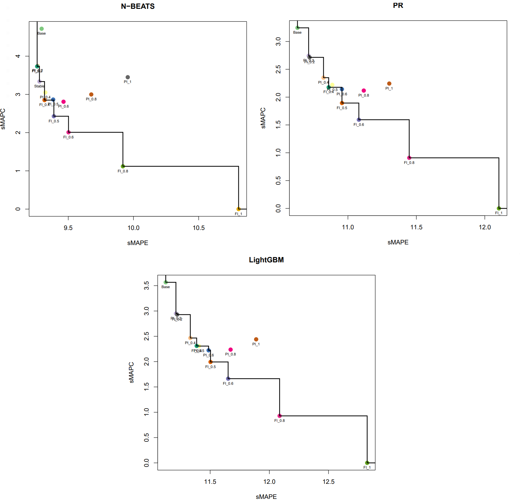
Figure 3: Pareto fronts showing the accuracy (sMAPE) and stability (sMAPC) of all vertical stability experimental models across the M4 dataset with N-BEATS, PR and LightGBM base models.

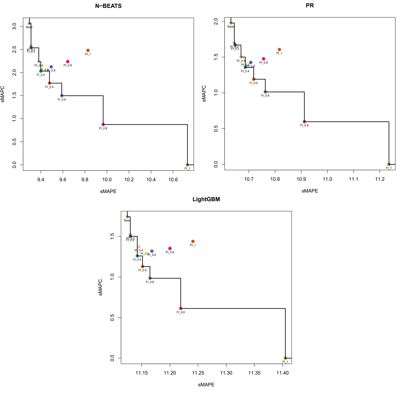
Figure 4: Pareto fronts showing the accuracy (sMAPE) and stability (sMAPC) of all horizontal stability experimental models across the M4 dataset with N-BEATS, PR and LightGBM base models.

Figures 3 and 4 show that there are no models that produce forecasts which are most accurate and stable at the same time with any base model. The Stable N-BEATS is on the Pareto front and thus, it is a good and valid method. However, it does not significantly stand out as there are other methods that are either more accurate or stable than the Stable N-BEATS. Hence, with our simpler interpolation approach, we can get comparable results. Furthermore, our method easily produces the full spectrum of the accuracy-stability trade-off whereas with the Stable N-BEATS approach, the users have to change the parameter, $\lambda$, and retrain the model multiple times to get the full spectrum which can be time-consuming. Presenting the full spectrum is usually important for practitioners to select a model based on their requirements. For example, regarding both vertical and horizontal stability experiments on all base models across the M4 dataset, PI_0.2 and FI_0.2 can be selected to obtain more accurate forecasts and FI_0.6 and FI_0.8 can be selected to obtain more stable forecasts.

Figures 5 and 6 show the Pareto fronts that represent the accuracy (sMAPE) and stability (sMAPC) results across the M5 dataset for vertical and horizontal stability experiments, respectively.

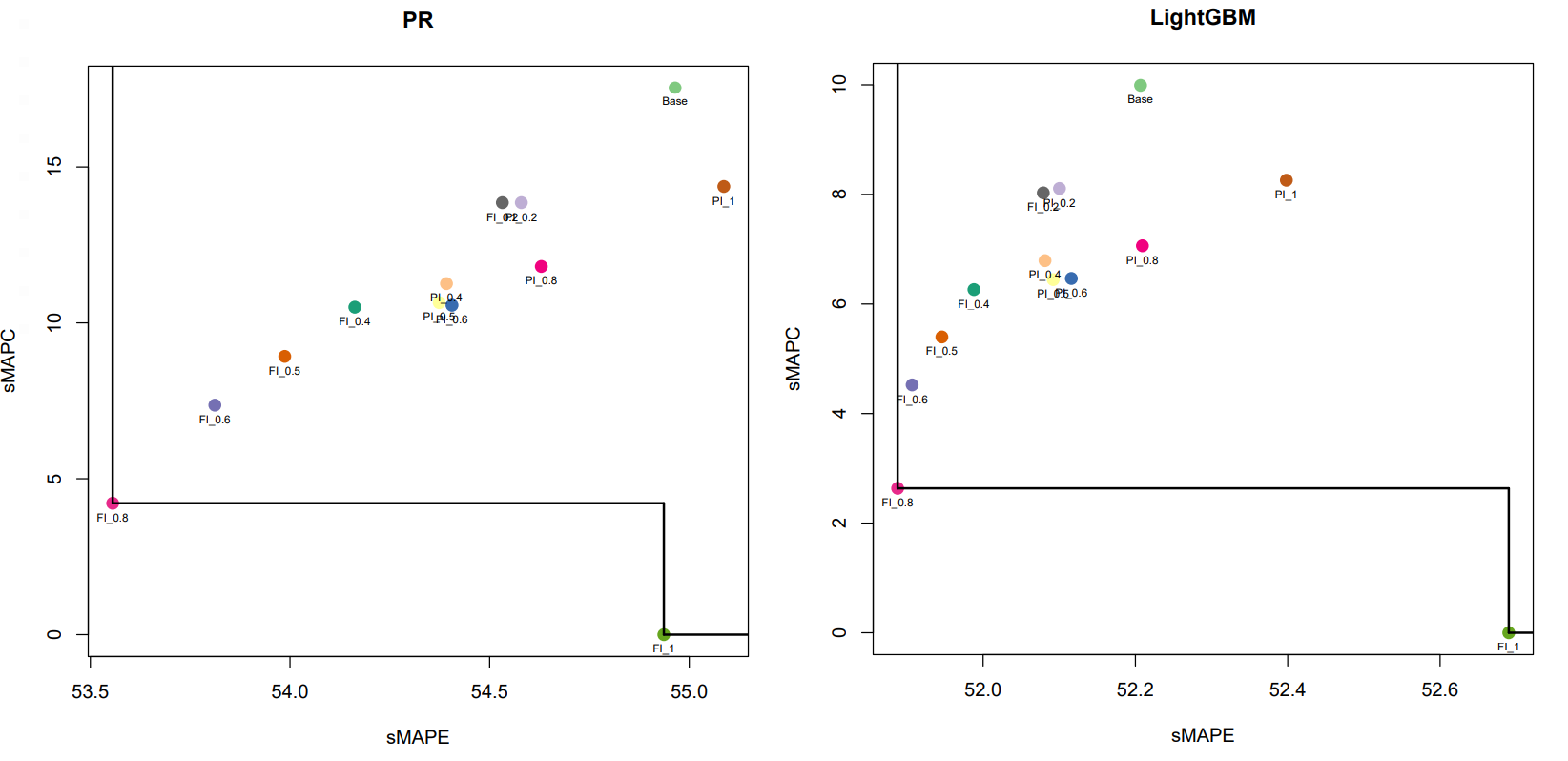
Figure 5: Pareto fronts showing the accuracy (sMAPE) and stability (sMAPC) of all vertical stability experimental models across the M5 dataset with PR and LightGBM base models.

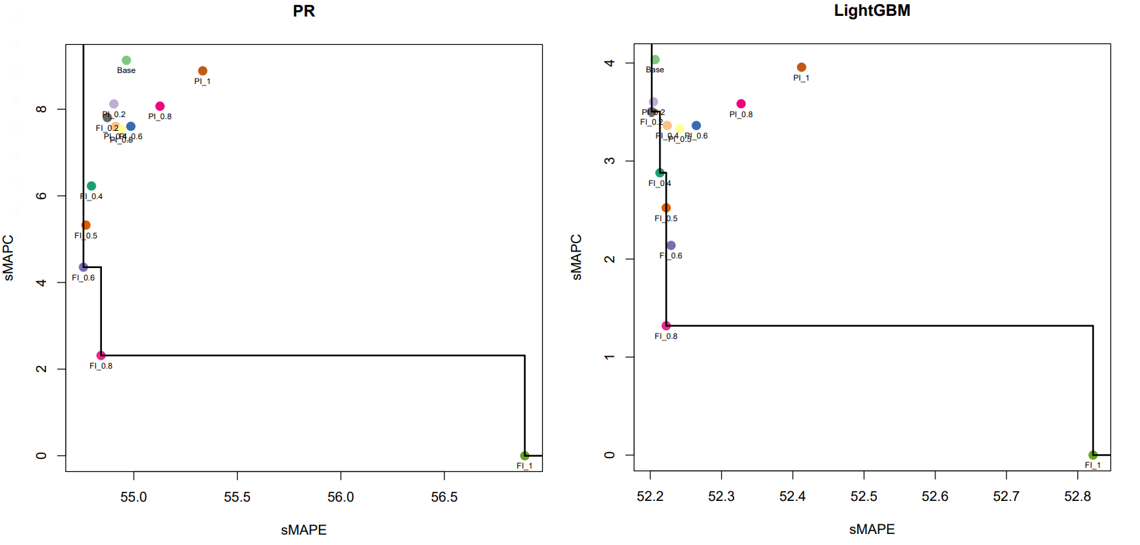
Figure 6: Pareto fronts showing the accuracy (sMAPE) and stability (sMAPC) of all horizontal stability experimental models across the M5 dataset with PR and LightGBM base models.

Here, the shapes of the Pareto fronts are considerably different from the Pareto fronts of the M4 dataset. In Figure 5, the variant FI_0.8 produces the most accurate forecasts across the M5 dataset with both PR and LightGBM models. This variant is also the second-best model in terms of stability. Thus, unlike with the M4 dataset, the FI_0.8 model variant can be used to obtain both accurate and vertically stable forecasts for the M5 dataset with both PR and LightGBM models. This phenomenon also explains the reason that the ensemble model proposed by In and Jung [8] won the M5 competition. The winning method also implicitly combines the forecasts obtained at different origins to produce the final forecasts and thus, the forecasts are stable and for this dataset, stable forecasts are also accurate. However, this does not work in the same way for any dataset and hence, presenting the full spectrum of accuracy-stability trade-off is highly useful for decision-making of real-world applications.

The observations are slightly different for the horizontal stability experiments across the M5 dataset. As shown in Figure 6, the FI_0.6 and FI_0.2 models respectively provide the most accurate forecasts with the PR and LightGBM models across the M5 dataset. However, these variants do not provide the most horizontally stable forecasts. Thus, in this case also the practitioners can select any model variant in the Pareto front based on their requirement to obtain forecasts. In general, the variant FI_0.8 provides considerably accurate and horizontally stable forecasts with both PR and LightGBM models. In both Figures 5 and 6, the base models are not on the Pareto fronts and this highlights that linear interpolation can produce both accurate and stable forecasts compared to the base models for the M5 dataset.

5 Conclusions and Future Research

Obtaining stable forecasts is highly important for many real-world applications. In this paper, we have systematically explored different types of stability, and have proposed a categorisation based on same/different targets and origins, focussing then on the two types of different origin and same target, and same origin and different target, that we call vertical stability and horizontal stability. Making the forecasts vertically stable across different forecast origins is important for correct decision-making and strategic planning. Also, making the forecasts horizontally stable across the forecast horizon can support reducing the bullwhip effect in supply chains. However, the area of stable forecasting has received limited attention in the forecast community. The available forecast stabilisation frameworks are only applicable to certain base models and extending those to stabilise the forecasts provided by any base model is not straightforward. Furthermore, these frameworks are only designed to make the forecasts vertically stable.

In this paper, we have proposed a simple model-agnostic linear interpolation approach to make the forecasts either vertically or horizontally stable. To make the forecasts made at a given origin vertically stable, the forecasts are linearly combined with the corresponding forecasts made at the previous origin. To make the forecasts horizontally stable across the forecast horizon, the adjacent forecasts are linearly combined. The proportion of the previous forecasts that is used during the interpolation to make the current forecasts is a parameter to the method that enables to easily control the trade-off between stability and accuracy. For both vertical and horizontal stability experiments, linear interpolation is conducted in two ways, partial interpolation and full interpolation. The experiments are conducted using three base models: N-BEATS, PR and LightGBM. Across four experimental datasets, we have shown that our framework can produce more stable forecasts compared to the benchmark models on six error metrics. Furthermore, our framework can produce more accurate and more stable forecasts for some datasets compared to the benchmark models on three error metrics.

From our experiments, we conclude that linear interpolation is a good approach to make the forecasts either vertically or horizontally stable. We further conclude that full interpolation leads to more stable forecasts compared to partial interpolation with both vertical and horizontal stability types as it considers the previously interpolated forecasts to make the next forecasts. For the datasets with intermittent series such as Favorita and M5, the full interpolation models can provide both more accurate and more stable forecasts than the base models. For the datasets with higher trends and seasonal effects such as M3 and M4, the full interpolation models can provide forecasts that only lose small amounts of accuracy in exchange for being considerably more stable. For those datasets, our apporach enables practitioners to select a trade-off between accuratcy and stability from the Pareto front, based on their requirements. Compared with other recently proposed forecast stability models, our interpolation based framework is simple to implement and it is applicable to any base model to make forecasts either vertically or horizontally stable. Thus, we recommend using our full interpolation framework as a benchmark and easy way to stabilise the forecasts, before potentially more sophisticated methods are tried.

There are many possible avenues to extend this research. Weighting mechanisms could be developed to change stability, in the case of horizontal stability with respect to trend, seasonality, holiday effects, known promotions, and other similar effects. Also different weighting for different horizons may be beneficial in certain situations. Finally, in the case of vertical stability, one point worthy of investigation would be to develop measures of how much new information the newly available data add. Though this is a problem at the core of any forecasting method, as in, how responsive it should to the most recent observations, this is also relevant in a stability context, as truly new information may render stability less desirable.

References

- Altavilla and Ciccarelli [2007] Altavilla, C., Ciccarelli, M., 2007. Information combination and forecast (st)ability: Evidence from vintages of time-series data: Technical report 846. European Central Bank (ECB) .
- Bates and Granger [1969] Bates, J.M., Granger, C.W., 1969. The combination of forecasts. Journal of the Operational Research Society 20, 451––468.
- Breiman [2001] Breiman, L., 2001. Random forests. Machine Learning 45, 5–32.
- Friedman et al. [2010] Friedman, J., Hastie, T., Tibshirani, R., 2010. Regularization paths for generalized linear models via coordinate descent. Journal of Statistical Software 33, 1–22.
- Gelman and Hill [2006] Gelman, A., Hill, J., 2006. Data analysis using regression and multilevel/hierarchical models. Analytical Methods for Social Research, Cambridge University Press.
- Godahewa et al. [2021] Godahewa, R., Bergmeir, C., Webb, G.I., Hyndman, R.J., Montero-Manso, P., 2021. Monash time series forecasting archive, in: Neural Information Processing Systems Track on Datasets and Benchmarks.
- Hewamalage et al. [2021] Hewamalage, H., Bergmeir, C., Bandara, K., 2021. Recurrent neural networks for time series forecasting: Current status and future directions. International Journal of Forecasting 37, 388–427.
- In and Jung [2022] In, Y., Jung, J.Y., 2022. Simple averaging of direct and recursive forecasts via partial pooling using machine learning. International Journal of Forecasting 38, 1386–1399. Special Issue: M5 competition.
- Kaggle [2018] Kaggle, 2018. Corporación favorita grocery sales forecasting. https://www.kaggle.com/c/favorita-grocery-sales-forecasting.
- Ke et al. [2017] Ke, G., Meng, Q., Finley, T., Wang, T., Chen, W., Ma, W., Ye, Q., Liu, T., 2017. LightGBM: A highly efficient gradient boosting decision tree, in: Proceedings of the 31st International Conference on Neural Information Processing Systems, Curran Associates Inc., Red Hook, NY, USA. p. 3149–3157.
- Ke et al. [2020] Ke, G., Soukhavong, D., Lamb, J., Meng, Q., Finley, T., Wang, T., Chen, W., Ma, W., Ye, Q., Liu, T.Y., 2020. lightgbm: light gradient boosting machine. URL: https://CRAN.R-project.org/package=lightgbm. R package version 3.1.1.
- Kolassa [2011] Kolassa, S., 2011. Combining exponential smoothing forecasts using akaike weights. International Journal of Forecasting 27, 238–251.
- Lee and Padmanabhan [1997] Lee, H.L., Padmanabhan, V.and Whang, S., 1997. Information distortion in a supply chain: The bullwhip effect. Management Science 43, 546–558.
- Li and Disney [2017] Li, Q., Disney, S.M., 2017. Revisiting rescheduling: MRP nervousness and the bullwhip effect. International Journal of Productions Research 55, 1992–2012.
- Makridakis and Hibon [2000] Makridakis, S., Hibon, M., 2000. The M3-competition: results, conclusions and implications. International Journal of Forecasting 16, 451–476.
- Makridakis et al. [2018] Makridakis, S., Spiliotis, E., Assimakopoulos, V., 2018. The M4 competition: results, findings, conclusion and way forward. International Journal of Forecasting 34, 802–808.
- Makridakis et al. [2022] Makridakis, S., Spiliotis, E., Assimakopoulos, V., 2022. The M5 accuracy competition: Results, findings and conclusions. International Journal of Forecasting 38, 1346–1364.
- Montero-Manso and Hyndman [2021] Montero-Manso, P., Hyndman, R.J., 2021. Principles and algorithms for forecasting groups of time series: Locality and globality. International Journal of Forecasting 37, 1632–1653.
- Oreshkin et al. [2020] Oreshkin, B.N., Carpov, D., Chapados, N., Bengio, Y., 2020. N-BEATS: Neural basis expansion analysis for interpretable time series forecasting, in: 8th International Conference on Learning Representations (ICLR).
- Rey and Neuhäuser [2011] Rey, D., Neuhäuser, M., 2011. International Encyclopedia of Statistical Science. Springer, Berlin, Heidelberg.
- Sammut and Webb [2010] Sammut, C., Webb, G.I. (Eds.), 2010. Encyclopedia of Machine Learning. Springer US, Boston, MA.
- Schapire [1999] Schapire, R.E., 1999. A brief introduction to boosting, in: Proceedings of the 16th International Joint Conference on Artificial Intelligence - Volume 2, Morgan Kaufmann Publishers Inc., San Francisco, CA, USA. p. 1401–1406.
- Schuster et al. [2017] Schuster, N., Ehm, H., Hottenrott, A., Lauer, T., 2017. Bridging short and mid-term demand forecasting in the semiconductor industry, in: 2017 Winter Simulation Conference, IEEE. p. 3658–3669.
- Timmermann [2006] Timmermann, A., 2006. Forecast combinations. Handbook of Economic Forecasting 1, 135–196.
- Tunc et al. [2013] Tunc, H., Kilic, O.A., Tarim, S.A., Eksioglu, B., 2013. A simple approach for assessing the cost of system nervousness. International Journal of Production Economics 141, 619–625.
- Van Belle et al. [2023] Van Belle, J., Crevits, R., Verbeke, W., 2023. Improving forecast stability using deep learning. International Journal of Forecasting 39, 1333–1350.
- Yuan and Yang [2005] Yuan, Z., Yang, Y., 2005. Combining linear regression models: When and how? Journal of the American Statistical Association 100, 1202–1214.