Grokking Beyond Neural Networks: An Empirical Exploration with Model Complexity

Abstract

In some settings neural networks exhibit a phenomenon known as grokking, where they achieve perfect or near-perfect accuracy on the validation set long after the same performance has been achieved on the training set. In this paper, we discover that grokking is not limited to neural networks but occurs in other settings such as Gaussian process (GP) classification, GP regression and linear regression. We also uncover a mechanism by which to induce grokking on algorithmic datasets via the addition of dimensions containing spurious information. The presence of the phenomenon in non-neural architectures provides evidence that grokking is not specific to SGD or weight norm regularisation. Instead, grokking may be possible in any setting where solution search is guided by complexity and error. Based on this insight and further trends we see in the training trajectories of a Bayesian neural network (BNN) and GP regression model, we make progress towards a more general theory of grokking. Specifically, we hypothesise that the phenomenon is governed by the accessibility of certain regions in the error and complexity landscapes.

1 Introduction

Grokking is intimately linked with generalisation. The phenomenon is characterised by a relatively quick capacity to perform well on a necessarily narrow training set, followed by an increase in more general performance on a validation set. In this paper, we explore grokking with reference to existing theories of generalisation and model complexity. In the introduction, we discuss these theoretical points and review existing work on grokking. Afterwards in Section 2, we present some novel empirical observations. Reflecting on these observations in Section 3, we hypothesise a general mechanism which explains grokking in settings where model selection is guided by error and complexity. Finally, in Section 4 we consider the limits of empirical evidence presented and what directions might be fruitful for further grokking research.

1.1 Generalisation

In abstract, generalisation is the capacity of a model to make good predictions in novel scenarios. To express this formally, we restrict our study of generalisation to supervised learning.

Definition 1.1 (Supervised Learning).

In supervised machine learning, we are given a set of training examples $X$, whose elements are members of $\mathcal{X}$, and associated targets $Y$, whose elements are members of $\mathcal{Y}$. We then attempt to find a function $f_{\theta}:\mathcal{X}\rightarrow\mathcal{Y}$ so as to minimise an objective function $\mathscr{L}:(X,Y,f_{\theta})\rightarrow\mathbb{R}$.

Having found $f_{\theta}$, we may look at the function’s performance under a possibly new objective function $\mathscr{G}$ (typically $\mathscr{L}$ without additional complexity considerations) on an unseen set of examples and labels, $X^{\prime}$ and $Y^{\prime}$. If $\mathscr{G}(X^{\prime},Y^{\prime})$ is small, we say that the model has generalised well and if it is large, it has generalised poorly.

1.2 Model Selection and Complexity

Consider $\mathscr{F}$, a set of models we wish to use for a prediction task. Presently, we have described a process by which to assess the generalisation performance of $f_{\theta}\in\mathscr{F}$ given $X^{\prime}$ and $Y^{\prime}$. Unfortunately, these hidden examples and targets are not available during training. As such, we may want to measure relevant properties about members of $\mathscr{F}$ that could be indicative of their capacity for generalisation. One obvious property is the value of $\mathscr{G}(X,Y)$ (or some related function) which we call the data fit. Another property is complexity. If we can find some means to measure the complexity, then traditional thinking would recommend we follow the principle of parsimony.

Definition 1.2 (Principle of Parsimony).

“[The principle of] parsimony is the concept that a model should be as simple as possible with respect to the induced variables, model structure, and number of parameters” ((Burnham and Anderson, 2004). That is, if we have two models with similar data fit, we should choose the simplest of the two.

If we wish to follow both the principle of parsimony and minimise the data fit, the loss function $\mathscr{L}$ we use for choosing a model is given by:

$$\mathscr{L}=\text{error}+\text{complexity}.$$ (1)

Suppose one is completing a regression task. In this case, if one substitutes error for mean squared error and complexity for the $L_{2}$ norm of the weights, we arrive at perhaps the most widely used loss function in machine learning:

$$\mathcal{L}=\frac{1}{N}\sum_{i=1}^{N}||f_{\theta}(x_{i})-y_{i}||^{2}+\frac{\beta}{M}\sum_{i=1}^{M}||\theta_{i}||^{2}.$$ (2)

where $N$ is the number of data samples, $M$ is the number of parameters and $\beta$ is a hyperparameter controlling the contribution of the weight decay term.

While Equation 1 may seem simple, it is often difficult to characterise the complexity term. Not only are there multiple definitions for model complexity across different model categories, definitions also change among the same category. When using a decision tree, we might measure complexity by tree depth and the number of leaf nodes ((Hu et al., 2021). Alternatively, for deep neural networks, we could count the number and magnitude of parameters or use a more advanced measure such as the linear mapping number (LMN) ((Liu et al., 2023a). Fortunately, in this wide spectrum of complexity measures, there are some unifying formalisms we can apply. One such formalism was developed by Kolmogorov ((Yueksel et al., 2020). In this formalism, we measure the complexity as the length of the minimal program required to generate a given model. Unfortunately, the difficulty of computing this measure makes it impractical. A more pragmatic alternative is the model description length. This defines the complexity of a model as the minimal message length required to communicate its parameters between two parties ((Hinton and van Camp, 1993).

1.2.1 Model Description Length

To understand model description length, we will consider two agents connected via a communication channel. One of these agents (Brian) is sending a model across the channel and the other (Oscar) is receiving the model. Both agree upon two items before communication. First, anything required to transmit the model with the parameters unspecified. For example, the software that implements the model, the training algorithm used to generate the model and the training examples (excluding the targets). Second, a prior distribution $P$ over parameters in the model . After initial agreement on these items, Brian learns a set of model parameters $\theta$ which are distributed according to $Q$. The complexity of the model found by Brian is then given by the cost of “describing” the model over the channel to Oscar. Via the “bits back” argument ((Hinton and van Camp, 1993), this cost is:

$$\mathcal{L}(f_{\theta})=D_{KL}(Q||P)$$ (3)

While the model description length is a relatively simple and quite general measure of model complexity, it relies upon a critical assumption. Namely, that the amount of information contained in the components agreed upon by Brian and Oscar should be small or shared among different models being compared. Fortunately, this is usually the case, especially in our experiments. When analysing the grokking phenomenon, we generally agree upon priors and look at the complexity of a model across epochs in optimisation. Thus, there is complete shared information cost outside of changes which occur during optimisation.

1.2.2 Minimal Description Length

The model description length is often combined with a data fit term under the minimal description length principle or MDL ((MacKay, 2003). One can understand this principle by considering the following scenario. Oscar does not know the training targets $Y$ but would like to infer them from $X$ to which he has access. To help Oscar, Brian transmits parameters $\theta$ which Oscar then uses to run $f_{\theta}$ on $X$. However, the model is not perfect; so Brian must additionally send corrections to the model outputs. The combined message of the corrections and model, denoted $(D,f)$, has a total description length of:

$$\mathcal{L}(D,f_{\theta})=\mathcal{L}(f_{\theta})+\mathcal{L}(D|f_{\theta}).$$ (4)

In reference to Equation 1, the model description length is taking the role of the complexity term and the residuals are taking on the role of the data fit. The model which minimises $\mathcal{L}(D,f_{\theta})$ is deemed optimal under the MDL principle ((Hinton and van Camp, 1993) and also under our generalised objective function in Equation 1.

Notably, the MDL principle is equivalent to two widely used paradigms for model selection. The first is MAP estimation from Bayesian inference where $\mathcal{L}(f_{\theta})$ comes to represent a prior over the parameters which specify $f_{\theta}$ ((MacKay, 2003). The second equivalence is with Equation 2. Indeed, if one calculates $L(D,f_{\theta})$ under a Gaussian prior and posterior where the standard deviation of these distributions are fixed in advance, the model complexity term reduces to a squared weight penalty and the data fit is proportional to the mean squared error ((Hinton and van Camp, 1993).

1.2.3 The Case of GP Regression

While the model description length is equivalent to many complexity measures used in model selection, it is not equivalent to all. For example, we complete some experimentation with GP regression where we observe grokking across optimisation of the kernel hyperparameters. The posterior distribution of these kernel parameters is given by:

$$p(\theta|X,y) =\frac{p(y|X,\theta)p(\theta)}{p(y|X)}=\frac{p(\theta)\int p(y|f,X)p(f|\theta)df}{p(y|X)}$$ (5)

From here we could use MAP-estimation to find $\theta$ which we know is equivalent to the MDL. However, it is standard practice in GP optimisation to find $\theta$ which maximises $p(y|X,\theta)$ ((Rasmussen and Williams, 2006). It turns out $p(y|X,\theta)$ itself contains a regularising term which is often labelled the complexity ((Rasmussen and Williams, 2006):

$$\log p(y|X,\theta)=-\underbrace{\frac{1}{2}y^{T}K_{\theta}^{-1}y}_{\text{data fit}}-\underbrace{\frac{1}{2}\log|K_{\theta}|}_{\text{complexity}}-\underbrace{\frac{n}{2}\log 2\pi}_{\text{normalisation}}.$$ (6)

In Equation 6, this so-called complexity penalty characterises “the volume of possible datasets that are compatible with the data fit term” ((Bauer et al., 2016). This is clearly distinct from the model description length. However, Equation 6 is still congruent with Equation 1 and thus amenable to later analysis in this paper. As we will see, even though this definition of complexity is not equivalent to the description length, it seems to serve the same function empirically and is treated in the same way by our grokking hypothesis.

1.3 The Grokking Phenomenon

The grokking phenomenon was recently discovered by Power et al. ((2022) and has garnered attention from the machine learning community. We define the phenomenon in Definition 1.3.

Definition 1.3 (Grokking).

Grokking is a phenomenon in which the performance of a model $f_{\theta}$ on the training set reaches a low error at epoch $E_{1}$, then following further optimisation, the model reaches a similarly low error on the validation dataset at epoch $E_{2}$. Importantly the value $\Delta_{k}=|E_{2}-E_{1}|$ must be non-trivial.

In many settings, the value of $\Delta_{k}$ is much greater than $E_{1}$. Additionally, the change from poor performance on the validation set to good performance can be quite sudden. A prototypical illustration of grokking is provided in Figure 13 (Appendix H.2).

Since initial publication by Power et al. ((2022), there has been empirical and theoretical exploration of the phenomenon. In Section 1.3.1, we summarise the experimentation completed and in Section 1.3.2, we discuss the current theories of grokking. Due to the phenomenon’s recent discovery, few theories exist which seek to explain it and those that do tend to focus on particular architectures. Further, the prevalence of grokking across the wide gamut of machine learning algorithms has not been thoroughly investigated.

1.3.1 Architectures and Datasets

To the best of our knowledge, all notable existing empirical literature on the grokking phenomenon is summarised in Table 1. The literature has focused primarily on neural network architectures and algorithmic datasets. No paper has yet demonstrated the existence of the phenomenon using a GP or linear regression. We believe that extension of the effect to these other machine learning models would be of interest to the community.

1.3.2 Theories of Grokking

Several theories have been presented to explain grokking. They can be categorised into two main classes based on the mechanism they use to analyse the phenomenon. Loss-based theories such as Liu et al. ((2023b) appeal to the loss landscape of the training and test sets under different measures of complexity and data fit. Alternatively, representation-based theories such as Davies et al. ((2023), Barak et al. ((2022), Nanda et al. ((2023) and Varma et al. ((2023) claim that grokking occurs as a result of representation learning (or circuit formation) and associated training dynamics. The current set of theories tend to be narrow and thus might not be applicable if grokking were found in non-neural architectures.

Loss based theory. Liu et al. ((2023b) assume that there is a spherical shell (Goldilocks zone) in the weight space where generalisation is better than outside the shell. They claim that, in a typical case of grokking, a model will have large weights and quickly reach an over-fitting solution outside of the Goldilocks zone. Then regularisation will slowly move weights towards the Goldilocks zone. That is, grokking occurs due to the mismatch in time between the discovery of the overfitting solution and the general solution. While some empirical evidence is presented in Liu et al. ((2023b) for their theory, and the mechanism itself seems plausible, the requirement of a spherical Goldilocks zone seems too stringent. It may be the case that a more complicated weight-space geometry is at play in the case of grokking.

Liu et al. ((2023a) also recently explored some cases of grokking using the LMN metric. They find that during periods they identify with generalisation, the LMN decreases. They claim that this decrease in LMN is responsible for grokking.

Representation or circuit based theory. Representation or circuit based theories require the emergence of certain general structures within neural architectures. These general structures become dominant in the network well after other less general ones are sufficient for low training loss. For example, Davies et al. ((2023) claim that grokking occurs when, “slow patterns generalize well and are ultimately favoured by the training regime, but are preceded by faster patterns which generalise poorly.” Similarly, it has been shown that stochastic gradient descent (SGD) slowly amplifies a sparse solution to algorithmic problems which is hidden to loss and error metrics ((Barak et al., 2022). This is mirrored somewhat in the work of Liu et al. ((2022) which looks to explain grokking via a slow increase in representation quality. Nanda et al. ((2023) claim in the setting of an algorithmic dataset and transformer architecture, training dynamics can be split into three phases based on the network’s representations: memorisation, circuit formation and cleanup. Additionally, that the structured mechanisms (circuits) encoded in the weights are gradually amplified with later removal of memorising components. Varma et al. ((2023) are in general agreement with Nanda et al. ((2023). Representation (or circuit) theories seem the most popular, based on the number of research papers published which use these ideas. They also seem to have a decent empirical backing. For example, Nanda et al. ((2023) explicitly discover circuits in a learning setting where grokking occurs.

2 Experiments

In the following section, we present various empirical observations we have made regarding the grokking phenomenon. In Section 2.1, we demonstrate that grokking can occur with GP classification and linear regression. This proves its existence in non-neural architectures, identifying a need for a more general theory of the phenomenon. Further, in Section 2.2, we show that there is a way of inducing grokking via data augmentation. Finally, in Section 2.3, we examine directly the weight-space trajectories of models which grok during training, incidentally demonstrating the phenomenon in GP regression. Due to their number, the datasets used for these experiments are not described in the main text but rather in Appendix C.

2.1 Grokking in GP Classification and Linear Regression

In the following experiments, we show that grokking occurs with GP classification and linear regression. In the case of linear regression, a very specific set of circumstances were required to induce grokking. However, for the GP models tested using typical initialisation strategies, we were able to observe behaviours which satisfy Definition 1.3. Such findings demonstrate that grokking is a more general phenomenon than previously demonstrated in the literature.

2.1.1 Zero-One Classification on a Slope with Linear Regression

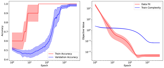
Figure 1: Accuracy, data fit and complexity on zero-one slope classification task with a linear model. Note that the shaded region corresponds to the standard error of five training runs.

As previously mentioned, to demonstrate the existence of grokking with linear regression, a very specific learning setting was required. We employed Dataset 9 with three additional spurious dimensions and two training points. Given a particular example $x_{0}$ from the dataset, the spurious dimensions were added as follows to produce the new example $x^{\prime}$:

$$x^{\prime}=\begin{bmatrix}x_{0}&x_{0}^{2}&x_{0}^{3}&\sin(100x_{0})\end{bmatrix}^{T}$$ (7)

The model was trained as though the problem were a regression task with outputs later transformed into binary categories based on the sign of the predictions. To find the model weights, we used SGD over a standard loss function with a MSE data fit component and a scaled weight-decay complexity term:

$$L=\frac{\text{MSE}(y,\hat{y})}{\epsilon_{0}}+\sum_{i=0}^{d}\frac{(w^{i}-\mu_{0}^{i})^{2}}{\sigma_{0}^{i}}.$$ (8)

In Equation 8, $i$ indexes the dimensionality of the variables $w_{0},\mu_{0}$ and $\sigma_{0}$, $\epsilon_{0}$ is the noise variance, $\mu_{0}$ is the prior mean, $\sigma_{0}$ is the prior variance, and $w$ is the weight vector of the model. For our experiment, $\mu_{i}$ was taken to be $0$ and $\sigma_{i}$ to be $0.5$ for all $i$. Regarding initialisation, $w$ was heavily weighted against the first dimension of the input examples. This unusual alteration to the initial weights was required for a clear demonstration of grokking with linear regression.

The accuracy, complexity and data fit of the linear model under five random seeds governing dataset generation is shown in Figure 1. Clearly, in the region between epochs $2\cdot 10^{1}$ and $10^{3}$, validation accuracy was significantly worse than training accuracy and then, in the region $2\cdot 10^{3}$, the validation accuracy was very similar to that of the training accuracy. This satisfies Definition 1.3, although the validation accuracy did not always reach $100\%$ in every case. Provided in Appendix F.1 is an example of a training run with a specific seed and a clearer case of grokking with $100\%$ accuracy.

2.1.2 Zero-One Classification with a Gaussian Process

In our second learning scenario, we applied GP classification to Dataset 8 with a radial basis function (RBF) kernel:

$$k(x_{1},x_{2})=\alpha\exp\left(-\frac{1}{2}(x_{1}-x_{2})^{T}\Theta^{-2}(x_{1}-x_{2})\right).$$ (9)

Here, $\Theta$ is called the lengthscale parameter and $\alpha$ is the kernel amplitude. Both $\Theta$ and $\alpha$ were found by minimising the approximate negative marginal log likelihood associated with a Bernoulli likelihood function via the Adam optimiser acting over the variational evidence lower bound ((Hensman et al., 2015; Gardner et al., 2018).

The result of training the model using five random seeds for dataset generation and model initialisation can be seen in Figure 2. The final validation accuracy is not $100\%$ like the cases we will see in the proceeding sections. However, it is sufficiently high to say that the model has grokked. In Appendix F.2, we also provide a plot of the model complexity as the KL divergence between the variational distribution and the prior for the training function values. As we later discuss in Section 4, there are issues with using this as a measure of complexity.

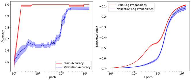
Figure 2: Accuracy and log likelihoods on zero-one classification task with a RBF Gaussian process. Note that the shaded region corresponds to the standard error of five training runs.

2.1.3 Parity Prediction with a Gaussian Process

In our third learning scenario, we also looked at GP classification. However, this time on a more complex algorithmic dataset – a modified version of Dataset 1 (with $k=3$) where additional spurious dimensions are added and populated using values drawn from a normal distribution. In particular, the number of additional dimensions is $n=37$ making the total input dimensionality $d=40$. We use the same training set up as in Section 2.1.2. The results (again with five seeds) can be seen in Figure 3 with a complexity plot in Appendix F.3 and discussion of the limitations of this complexity measure in Section 4.

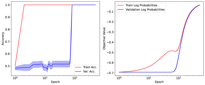
Figure 3: Accuracy and log likelihoods on hidden parity prediction task with RBF Gaussian process. Note that the shaded region corresponds to the standard error of five training runs. Acc. is Accuracy and Val. is Validation.

2.2 Inducing Grokking via Concealment

In this section, we investigate how one might augment a dataset to induce grokking. In particular, we develop a strategy which induces grokking on a range of algorithmic datasets. This work was inspired by Merrill et al. ((2023) and Barak et al. ((2022) where the true task is “hidden” in a higher dimensional space. This requires models to “learn” to ignore the additional dimensions of the input space. For an illustration of learning to ignore see Figure 12 (Appendix H.1).

Our strategy is to extend this “concealment” idea to other algorithmic datasets. Consider $(x,y)$, an example and target pair in supervised learning. Under concealment, one augments the example $x$ (of dimensionality $d$) by drawing $v\sim\mathcal{N}(0,I_{l})$ and appending it to $x$. The new concealed example $x^{\prime}$ is:

$$x^{\prime}=\begin{bmatrix}x_{0}&x_{1}&\cdots&x_{d}&v_{0}&\cdots&v_{l}\end{bmatrix}^{T}.$$

To determine the generality of this strategy in the algorithmic setting, we applied it to 6 different datasets (2-7). These datasets were chosen as they share a regular form and seem to cover a fairly diverse variety of algorithmic operations. In each case, we used the prime $7$, and varied the additional dimensionality $k$. For the model, we used a simple neural network analogous to that of Merrill et al. ((2023). This neural network consisted of $1$ hidden layer of size $1000$ and was optimised using SGD with cross-entropy loss. The weight decay was set to $10^{-2}$ and the learning rate to $10^{-1}$.

To discover the relationship between concealment and grokking, we measured the “grokking gap” $\Delta_{k}$ as presented in Definition 1.3. In particular, we considered how an increase in the number of spurious dimensions relates to this gap. The algorithm used to run the experiment is detailed in Algorithm 1 (Appendix G.1). The result of running this algorithm can be seen in Figure 4. In addition to visual inspection of the data, a regression analysis was completed to determine whether the relationship between grokking gap and additional dimensionality might be exponential. The result of this regression is denoted as Regression Fit in the figure.

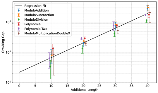
Figure 4: Relationship between grokking gap and number of additional dimensions using the grokking via concealment strategy. Note that $x$-values are artificially perturbed to allow for easier visibility of error bars. In reality they are either $10$, $20$, $30$ or $40$. Also, the data of zero additional length is removed (although still influences the regression fit). See Appendix G.2 for the plot without these changes.

The Pearson correlation coefficient ((Pearson, 1895) was also calculated in log space for all points available and for each dataset individually. Further, we completed a test of the null hypothesis that the distributions underlying the samples are uncorrelated and normally distributed. The Pearson correlation $r$ and $p$-values are presented in Table 2 (Appendix D.2) The Pearson correlation coefficients are high in aggregate and individually, indicating a positive linear trend in log space. Further, $p$ values in both the aggregate and individual cases are well below the usual threshold of $\alpha=0.05$.

2.3 Parameter Space Trajectories of Grokking

Our last set of experiments was designed to interrogate the parameter space of models which grok. We completed this kind of interrogation in two different settings. The first was GP regression on Dataset 10 and the second was BNN classification on a concealed version of Dataset 1. Since the GP only had two hyperparameters governing the kernel, we could see directly the contribution of complexity and data fit terms. Alternatively, for the BNN we aggregated data regarding training trajectories across several initialisations to investigate the possible dynamics between complexity and data fit.

2.3.1 GP Grokking on Sinusoidal Example

In this experiment, we applied a GP (with the same kernel as in Section 2.1.2) to regression of a sine wave. To find the optimal parameters for the kernel, a Gaussian likelihood function was employed with exact computation of the marginal log likelihood. In this optimisation scenario, the complexity term is as described in Section 1.2.3.

To see how grokking might be related to the complexity and data fit landscapes, we altered parameter initialisations. We considered three different initialisation types. In case A, we started regression in a region of high error and low complexity (HELC) where a region of low error and high complexity (LEHC) was relatively inaccessible when compared a region of low error and low complexity (LELC). For case B, we initialised the model in a region of LEHC where LELC solutions were less accessible. Finally, in case C, we initialised the model in a region of LELC.

As evident in Figure 5, we only saw grokking for case B. It is interesting that, in this GP regression case, we did not see a clear example of the spherical geometry mentioned in the Goldilocks zone theory of Liu et al. ((2023b). Instead a more complicated loss surface is present which results in grokking.

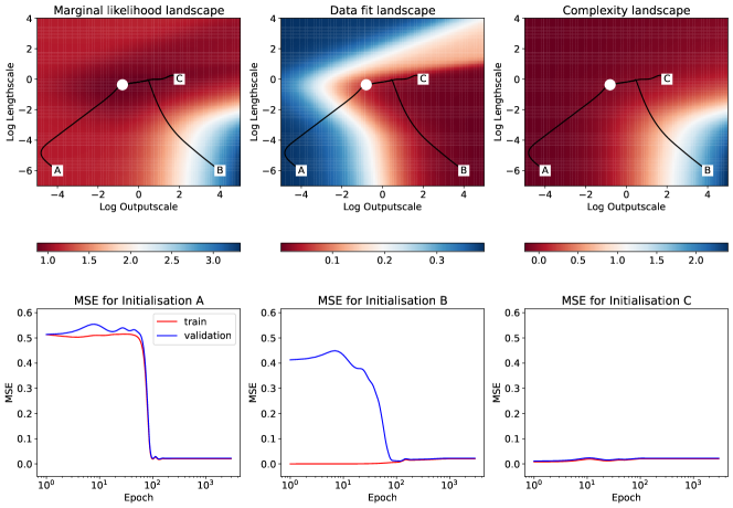
Figure 5: Trajectories through parameter landscape for GP regression. Initialisation points A-C refer to those mentioned in Section 2.3.1.

2.3.2 Trajectories of a BNN with Parity Prediction

We also examined the weight-space trajectories of a BNN ($f_{\theta}$). Our learning scenario involved Dataset 1 with the concealment strategy presented in Section 2.2. Specifically, we used an additional dimensionality of $27$ and a parity length of $3$. To train the model, we employed SGD with the following variational objective:

$$\begin{split}\mathcal{L}(\phi)=\mathbb{E}_{Q_{\phi}(\theta)}[\text{CrossEntropyLoss}(f_{\theta}(X),Y)]+D_{KL}(Q_{\phi}(\theta)||P(\theta))\end{split}$$ (10)

In Equation 10, $P(\theta)$ is a standard Gaussian prior on the weights and $Q_{\phi}(\theta)$ is the variational approximation. The complexity penalty in this case is exactly the model description length discussed in Section 1.2 with the overall loss function clearly a subset of Equation 1.

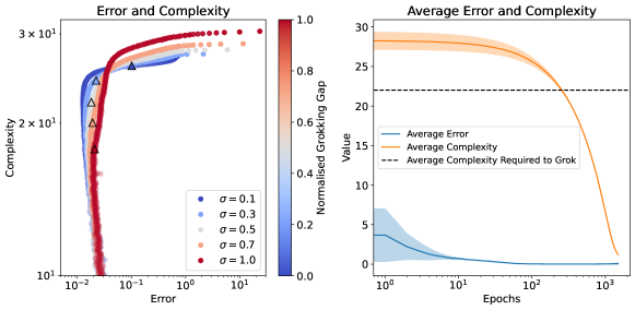
Figure 6: Grokking with BNN using different standard deviation values ($\sigma$) for the variational mean initialisations. Normalised Grokking Gap refers to the difference in epoch between high training accuracy and high validation accuracy normalised between zero and 1. In the left-hand plot, the transparency of a point indicates at which epoch it was recorded (more transparent equates to further in training) and triangles of a particular colour correspond to the point on the error-complexity landscape at which a model with a particular initialisation exhibited grokking. Note that three trials were run per $\sigma$ initialisation.

To explore the weight-space trajectories of the BNN we altered the network’s initialisation by changing the standard deviation of the normal distribution used to seed the variational mean of the weights. This resulted in network initialisations with differing initial complexity and error. We then trained the network based on these initialisations using three random seeds, recording values of complexity, error and accuracy. The outcomes of this process are in Figure 6. Notably, initialisations which resulted in an increased grokking gap correlate with increased optimisation time in regions of LEHC. Further, there seems to be a trend across epochs with error and complexity. At first, there is a significant decrease in error followed by a decrease in complexity.

3 Grokking and Complexity

Thus far we have explored grokking with reference to different complexity measures across a range of models. We have found the existence of the phenomenon in GP classification and regression, linear regression and BNNs. We have identified a means to induce grokking via the addition of spurious dimensions. Finally, we have analysed the trajectories of a GP and BNN during training, observing trends associated with the complexity and error of the models. Noting the discussion in Section 1.3.2, there seems to be no theory of grokking in the literature which can explain the new empirical evidence we present. Motivated by this, we construct a new hypothesis which fills this gap. We believe this hypothesis to be compatible with our new results, previous empirical observations and with many previous theories of the grokking phenomenon.

To build the hypothesis, we first make Assumption 1. We then posit Claim 1, our hypothesis of grokking, which we sometimes refer to as the complexity theory of grokking.

Assumption 1.

For the task of interest, the principle of parsimony holds. That is, solutions with minimal possible complexity will generalise better.

Claim 1.

If the low error, high complexity (LEHC) weight space is readily accessible from typical initialisation but the low error, low complexity (LELC) weight space is not, models will quickly find a low error solution which does not generalise. Given a path between LEHC and LELC regions which has non-increasing loss, solutions in regions of LEHC will slowly be guided toward regions of LELC due to regularisation. This causes an eventual decrease in validation error, which we see as grokking.

3.1 Explanation of Previous Empirical Results

In the following subsection, we demonstrate the congruence between our hypothesis and existing empirical observations. In Appendix E we draw parallels between our work and existing theory.

Learning with algorithmic datasets benefits from the principle of parsimony as a small encoding is required for the solution. In addition, when learning on these datasets, there appear to be many other more complex solutions which do not generalise but attain low training error. For example, with a neural network containing one hidden layer completing a parity prediction problem, there is competition between dense subnetworks which are used to achieve high accuracy on the training set (LEHC) and sparse subnetworks (LELC) which have better generalisation performance ((Merrill et al., 2023). In this case, the reduced accessibility of LELC regions compared to LEHC regions seems to cause the grokking phenomenon. This general story is supported by further empirical analysis completed by Liu et al. ((2022) and Nanda et al. ((2023). Liu et al. ((2022) found that a less accessible, but more general representation, emerges over time within the neural network they studied and that after this representation’s emergence, grokking occurs. Nanda et al. ((2023) discovered that a set of trigonometric identities were employed by a transformer to encode an algorithm for solving modular arithmetic. Additionally, this trigonometric solution was gradually amplified over time with the later removal of high complexity “memorising” structures. In this case, the model is moving from an accessible LEHC region where memorising solutions exist to a LELC region.

The work by Liu et al. ((2023b) showed the existence of grokking on non-algorithmic datasets via alteration of the initialisation and dataset size. From Claim 1, we can see why these factors would alter the existence of grokking. Changing the initialisation alters the relative accessibility of LEHC and LELC regions and reducing the dataset size may lessen constraints on LEHC regions which otherwise do not exist.

3.2 Explanation of New Empirical Evidence

Having been proposed to explain the empirical observation we have uncovered in this paper, Claim 1 should be congruent with these new findings – the first of which is the existence of grokking in non-neural models. Indeed, one corollary of our theory (Corollary 1) is that grokking should be model agnostic. This is because the proposed mechanism only requires certain properties of error and complexity landscapes during optimisation. It is blind to the specific architecture over which optimisation occurs.

Corollary 1.

The phenomenon of grokking should be model agnostic. Namely, it could occur in any setting in which solution search is guided by complexity and error.

Another finding from this paper is that of the concealment data augmentation strategy. We believe this can be explained via the lens of Claim 1 as follows. When dimensions are added with uninformative features, there exist LEHC solutions which use these features. However, the number of LELC solutions remains relatively low as the most general solution should have no dependence on the additional components. This leads to an increase in the relative accessibility of LEHC regions when compared to LELC regions which in turn leads to grokking.

4 Discussion

Despite some progress made toward understanding the grokking phenomenon in this paper, there is still some points to discuss. We should start by assessing the limitations of the empirical evidence gathered. This is important for a balanced picture of the experimentation completed and its implications for our grokking hypothesis. Having examined these limitations, we can provide some recommendations regarding related future work in the field.

4.1 Limitations of Empirical Evidence

In Section 2.1, experimentation with linear regression may be criticised for the specificity of the learning setup required to demonstrate grokking and for the value of the final validation accuracy. We note that the first critique is not reasonable in the sense that we should be able to show grokking under “normal” circumstances since grokking does not appear under “normal circumstances.” However, if one wanted to show that Claim 1 is a general theory of grokking, we should be able to see it at work in any learning setting which exhibits grokking. It could be the case that, with only one setting, we saw results consistent with Claim 1 but under another learning scenario, our claim could be proven false. We do not consider the second critique to be significant. For our purposes, grokking need not have $100\%$ accuracy as not all general solutions provide that. However, if this is desired, we provide a case where this occurs in Appendix F.1.

There are also reasonable critiques concerning the experimentation completed on GP classification. The most pressing might be concerns over the measurement of complexity as presented in Appendices F.2 and F.3. This is due to the way the model is optimised. Namely, via maximisation of the evidence lower bound:

$$\mathcal{L}_{\text{ELBO}}(\phi,\theta)=\sum_{i=1}^{N}\mathbb{E}_{q_{\phi}(f_{i})}[\log p(y_{i}|f_{i})]-\beta\text{KL}[q_{\phi}(f)||p_{\theta}(f)].$$ (11)

Unfortunately, optimisation of this value leads to changes in both the variational approximation and the hyperparameters of the prior GP. This presents a problem when trying to use the results of GP classification to validate Claim 1. The hyperparameters control the complexity of the prior which then influences the measured complexity of the model via the KL divergence. Consequently, the complexity measurement at any two points in training are not necessarily comparable. To disentangle optimisation of the hyperparameters and the variational approximation, one could complete a set of ablation studies. For this, one would keep either the hyperparameters or the variational approximation constant and alter the other variable. By doing so, one would be able to validate more directly Claim 1 with GP classification. Additionally, one might need to alter the learning setting to retain grokking under a new approximation scheme such as Laplace’s method. Further discussion and experimentation are provided in Appendix I.

Due to the simplicity of the model considered in Figure 5, it is hard to criticise experimentation completed there. However, the experimental design of the BNN lacks generality. Indeed, it is difficult to know if the subspace from which the BNN was initialised is indicative of general trends about the weight space. However, the values chosen were indicative of typical initialisation values. Thus, we can say that for “normal” cases that might be encountered by a practitioner, the BNN weight trajectories are representative.

4.2 Future Work

An interesting outcome of experimentation in this paper was the discovery of the concealment data augmentation strategy. As far as the authors are aware, this is the first data augmentation strategy found which consistently results in grokking. Additionally, its likely exponential trend with the degree of grokking is of great interest. Indeed, we know that the volume of a region in an $n$-dimensional space decreases exponentially with an increase in $n$. This fact and the exponential increase in grokking with additional dimensionality could be connected. Unfortunately, at this point in time, such a connection is only speculative. Thus, a more theoretical analysis might be warranted which seeks to examine this relationship.

5 Conclusion

We have presented novel empirical evidence for the existence of grokking in non-neural architectures and discovered a data augmentation technique which induces the phenomenon. Relying upon these observations and analysis of training trajectories in a GP and BNN, we proposed an effective theory of grokking. Importantly, we argued that this theory is congruent with previous empirical evidence and many previous theories of grokking. In future, researchers could extend the ideas in this paper by undertaking a theoretical analysis of the concealment strategy discovered and by testing the theory in non-algorithmic datasets.

Acknowledgements

We would like to acknowledge Russell Tsuchida, Matthew Ashman, Rohin Shah and Yuan-Sen Ting for their useful feedback on the content of this paper.

Supporting Information

All experiments can be found at this GitHub page. They have descriptive names and should reproduce the figures seen in this paper. For Figure 6, the relevant experiment is in the feat/info-theory-description branch.

Appendix A Summary of Existing Empirical Work on Grokking

Research Paper	Architecture	Category	Dataset Description
Power et al. [2022]	Transformer	Algorithmic	Problems of the form $a\circ b=c$ where $\circ$ is a binary operation and “$a$”, “$b$”, “$\circ$”, “$=$” and “$c$” are tokens.
Žunkovič and Ilievski [2022]	Perceptron Tensor Network	Rules-Based	1D cellular automaton rule, 1D exponential and $D$-dimensional uniform ball.
Liu et al. [2022]	MLP Transformer	Algorithmic Image class.	Addition modulo $P$, regular addition and MNIST.
Nanda et al. [2023]	Transformer	Algorithmic	Addition modulo $P$.
Liu et al. [2023b]	MLP LSTM GCNN	Algorithmic Image class. Language Molecules	Regular addition, MNIST, IMDb dataset and QM9.
Merrill et al. [2023]	MLP	Algorithmic	Modular addition.
Davies et al. [2023]	Transformer	Algorithmic	Addition modulo $P$.
Barak et al. [2022]	MLP Transformer PolyNet	Algorithmic	Parity prediction task.
Murty et al. [2023]	Transformer	Language	Question formation, tense-inflection and bracket nesting
Liu et al. [2023a]	MLP	Algorithmic	XOR, S4 group operation and bitwise XOR.
Varma et al. [2023]	Transformer	Algorithmic	Similar to Power et al. [2022]

Table 1: Summary of datasets and architectures in which the grokking phenomenon has been studied. Note that class. is short for classification.

Appendix B Kolmogorov Complexity

The Kolmogorov complexity is one of several measures of complexity discussed in this paper. In some sense, it is the measure of complexity with the least prior knowledge used to generate its value.

Definition B.1 (Kolmogorov).

According to Yueksel et al. [2020], the Kolmogorov complexity $K_{U}$ of a string $x$ with respect to a universal computer $U$ is:

$$K_{U}(x)=\min_{p:U(p)=x}l(p)$$ (12)

where $p$ denotes a program and $l(p)$ is the length of the program in some standard language.

Essentially, the Kolmogorov complexity is the length of the minimal program required to produce a string representation of a model. To illustrate this point, consider the three strings presented in Figure. 7. Let us assume that each of the associated programs are minimal under some language understood by a universal computer $U$. In this case, the first string would have the least complexity as the program specifying it requires $52$ characters, the second string would be more complex requiring $105$ and the third would be most complex requiring $106$. In the Kolmogorov formalism, if we have members $f,h\in\mathscr{F}$ and the minimal program to produce the string representation of $f$ is longer than $h$, it is more complex.

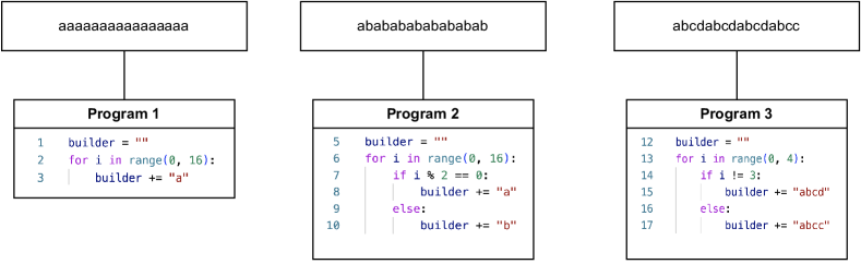
Figure 7: Illustration of Kolmogorov Complexity

With this Kolmogorov measure of complexity we can formalism the principle of parsimony under a computational picture. To do so, we use Solomonoff’s theory of inductive inference. In Solomonoff induction, we assume that we have an observation about the world $o\in\mathscr{O}$ which can be encoded in a binary string. In addition, we have a set of hypothesis $\mathscr{H}$ about that observation. We assume that these hypothesises are computable in the sense that each can be run on a Turing machine producing $o$. Further, we make a metaphysical assumption that true hypothesises are generated randomly using an unbiased process whereby the binary sequence defining $h\in\mathscr{H}$ is generated by choosing between three options at every point in the sequence: $0$, $1$ or END. In this setting if a hypothesis $h$ generates an observation $o$ but has a smaller Kolmogorov complexity than other hypotheses generating $o$, it is more likely [Altair, 2012].

B.1 Approximating Kolmogorov Complexity using Entropy

Unfortunately, the Kolmogorov complexity of a string (here a model) is non-computable [Vitányi, 2020]. However, we can approximate it with a concept from information theory [Shannon, 1948]. Namely, the entropy of a stochastic process which produces that string (or model).

Theorem 1.

Let a stochastic process $\{X_{i}\}$ be drawn i.i.d. according to the probability mass function $f(x)$, $x\in\mathcal{X}$, where $\mathcal{X}$ is a finite alphabet. According to Cover and Thomas [2006], we have the limit:

$$\frac{1}{n}\mathbb{E}\left[K(X^{n}|n)\right]\rightarrow H(X).$$ (13)

I.e. the expected Kolmogorov complexity of a $n$-bit string approaches the entropy of the distribution from which characters in that string are drawn.

Thus, if we treat each parameter of a model as a random variable, we may calculate the approximate Kolmogorov complexity of the model by considering the entropy of the distribution over the parameters which make up the model. For example, if we assume that each parameter $W$ in a particular model ($f$) is distributed normally, then the approximate distribution (after quantisation) for $W$ is given in Equation 14 [Hinton and van Camp, 1993]:

$$p(W)=\frac{t}{\sqrt{2\pi}}\exp\left[-\frac{W^{2}}{2}\right].$$ (14)

Now that we have a distribution over $W$, we can calculate $H(W)$:

$$H(W) =\mathbb{E}_{p}\left[-\ln p(W)\right]$$

$$=\mathbb{E}_{p}\left[-\ln\left(t\frac{1}{\sqrt{2\pi}}\exp\left[-\frac{W^{2}}{2}\right]\right)\right]$$

$$=\frac{1}{2}\mathbb{E}_{p}[W^{2}]+\text{const.}$$

Given this expression for $H(W)$, the approximate Kolmogorov complexity is then:

$$K(f)\approx\frac{N}{2}\mathbb{E}_{W}[W^{2}]+\text{const.}$$ (15)

Notably, $K(f)$ is proportional to the square of the weights of the network. Consequently, by minimising the approximate Kolmogorov complexity under the assumption of normality, we also minimise the $L_{2}$ norm of the weights. This is equivalent to the familiar weight decay regularisation strategy.

B.2 Connection Between Kolmogorov Complexity and Bayesianism

We can also relate Kolmogorov complexity to Bayesian inference. Consider the case where we are finding parameters of a model using the maximum a posteriori estimator. In this paradigm, we wish to choose the model $f_{\theta}$ to maximise $P(f|D)$ where $D$ is the data. According to Vitányi and Li [2000], this is equivalent to finding $\theta^{*}$ such that:

$$f_{\theta}^{*} =\min_{\theta}\left\{-\log P(D|f_{\theta})-\log P(f_{\theta})+\log P(D)\right\}$$ (16)

$$=\min_{\theta}\left\{-\log P(D|f_{\theta})-\log P(f_{\theta})\right\}$$

If we assume our hypothesis class to be finite and take the universal prior $m$, we can make the substitution $-\log P(f_{\theta})=K(f_{\theta})$ and $-\log P(D|f_{\theta})=K(D|f_{\theta})$ [Vitányi and Li, 2000]. This gives:

$$f_{\theta}^{*}=\min_{H}\left\{K(f_{\theta})+K(D|f_{\theta})\right\}.$$ (17)

Hence, under the universal prior, the maximum a posteriori estimator is equivalent to the minimiser of the Kolmogorov complexity of the model and of the data given the model.

Appendix C Datasets used in Experimentation

Many datasets were used for the experimentation completed in this paper. They are were either found in Merrill et al. [2023], Power et al. [2022] or were developed independently. Although grokking has been seen on non-algorithmic datasets [Liu et al., 2023b], we restrict ourselves to these and a basic regression task since our focus is a theoretical exploration of the phenomenon via the modification of other inducing variables. Work on larger datasets may have hindered this exploration.

Dataset 1 (Parity Prediction Task).

In the parity prediction task, the model is provided with a binary sequence $x$ of length $k$. The target $y$ is the parity of the sequence i.e. the product of the sequence if $0$ is $-1$ and $1$ is $1$.

Dataset 2 (Prime Modulo Addition Task).

In the prime modulo addition task, a prime $p$ and two numbers in the range $[0,p)$ are chosen. These numbers are represented by a one hot encoding and the model must predict their addition modulo $p$.

Dataset 3 (Prime Modulo Subtraction Task).

The prime modulo subtraction task has the same setup as Dataset 2, but is subtraction.

Dataset 4 (Prime Modulo Division Task).

The prime modulo division task has the same setup as Dataset 2, but is division.

Dataset 5 (Prime Modulo Polynomial Task).

The prime polynomial division task has the same setup as Dataset 2, but the model tries to predict the result of the equation:

$$x\circ y=x^{2}+xy+y^{2}\mod p$$ (18)

Dataset 6 (Extended Prime Modulo Polynomial Task).

The extended prime polynomial division task has the same setup as Dataset 2, but the model tries to predict the result of the equation:

$$x\circ y=x^{2}+xy+y^{2}+x\mod p$$ (19)

Dataset 7 (Extended Prime Modulo Multiplication Task).

The extended prime polynomial division task has the same setup as Dataset 2, but the model tries to predict the result of the equation:

$$x\circ y=x\cdot y\cdot x\mod p$$ (20)

Dataset 8 (1-0 Classification).

In this classification task, a model is attempting to distinguish whether a point will take a value of $0$ or $1$. These points are normally distributed (with $\sigma=1$) around $0$ and have label $y=0$ if they are below $x=0$ and $y=1$ if they are above.

Dataset 9 (1-0 Classification on a Slope).

In this classification task, a model is attempting to distinguish whether a point will is above $0$ or not. The $x$ values of these points are normally distributed (with $\sigma=1$) around $0$ and the $y$ values are given by the linear equation:

$$y=0.3x$$ (21)

Dataset 10 (Regression on a Sine Wave).

In this regression task, a model is attempting to predict the value of the equation:

$$y=A\sin(2\pi fx+\phi)+B\epsilon$$ (22)

where by default $A=1$, $f=\frac{1}{\pi}$, $\phi=0$, $B=0.1$ and $\epsilon$ is noise distributed according to $\mathscr{N}(0,1)$. Further $x$ values in the training set are modified so that the function is not necessarily on a uniform support by adding Gaussian noise of the same form as $\epsilon$.

Appendix D Statistical Analysis of the Concealment Strategy

D.1 Regression Method

Given a matrix $X$ of pairs $(l,\delta)$ where $l$ is the additional length and $\delta$ is the recorded grokking gap, we first transform the $y$-values into log space. That is, the dataset of pairs is given by:

$$X^{\prime}=\begin{bmatrix}X_{0}&\ln X_{1}\end{bmatrix}$$ (23)

Then we find the optimal coefficients $a$ and $b$ such that the model:

$$\hat{y}=aX^{\prime}_{0}+b$$ (24)

has minimal squared error with respect to the labels $X^{\prime}_{1}$. Returning from log to regular space, the function:

$$\delta=\exp\left(al+b\right)$$ (25)

is then our proposed relationship between additional dimensionality and grokking gap.

D.2 Correlation and $p$-Value Results

Dataset	$r$	$p$
Combined	$0.92$	$1.46\cdot 10^{-37}$
Addition	$0.933$	$3.91\cdot 10^{-7}$
Subtraction	$0.914$	$1.84\cdot 10^{-6}$
Division	$0.967$	$4.659\cdot 10^{-9}$
Polynomial	$0.959$	$1.860\cdot 10^{-8}$
Extended Polynomial	$0.906$	$2.981\cdot 10^{-6}$
Extended Multiplication	$0.942$	$1.484\cdot 10^{-7}$

Table 2: Table summarising the Person correlation $r$ and null hypothesis likelihood $p$ for concealment data in log space. Note that all datasets are under a modulo argument.

Appendix E Connection Between the Complexity Theory of Grokking and Previous Theories

The complexity theory of grokking unifies loss and representation based theories of grokking under a single framework. In the text below, we show how each may be seen as an example of the behaviour described in Claim 1.

The loss-based explanation of Liu et al. [2023b] asserts that in the weight space of a model there exists a Goldilocks zone of high generalisation. In cases of grokking, models will quickly find over-fitting solutions before being guided towards this Goldilocks zone via weight decay. As previously mentioned, weight norm can be seen as a measure of a model’s description length. Thus the guidance of weight norm is towards regions of lower complexity. Additionally, via Assumption 1, we can say that the Goldilocks zone must be a region of LELC since good generalisation comes from lower complexity. Consequently, this theory can be viewed as an instance of our broader framework with over-fitting solutions constituting LEHC and the Goldilocks zone constituting LELC.

The use of the LMN by Liu et al. [2023a] is also congruent with our theory of grokking. In the paper, the authors introduce LMN as a complexity measure and show that a decrease in LMN after a period of high training performance leads to a grokking solution. Under Claim 1, LMN is one instance of a complexity measure which can result in grokking.

Theories which use representation dynamics as a means of explaining grokking can also be placed in our framework. Via Assumption 1, more general representations should have a relatively low complexity. Thus, representation descriptions which talk of an emergence of general structures after the initial creation of memorising structures are talking of a transition from LEHC to LELC. Indeed, in neural networks it may be the case that LEHC solutions can often be characterised as “memorising” and LELC as “general circuits.” However, in other models we require the more abstract language of Claim 1.

Appendix F Additional Model Experiments

F.1 Linear Regression with a Specific Seed

In the following experiment, we take the same learning setting as in Section 2.1.1 but restrict ourselves to one seed which shows a clear case of grokking. This case is presented in Figure 8

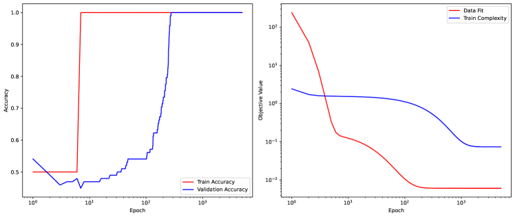
Figure 8: Accuracy, complexity and data fit on zero-one slope classification task with a linear model and one seed.

F.2 GP Classification Complexity for 0-1 Classification

We take the same learning setting as in Section 2.1.2, showing the complexity and error curves in Figure 9. In this figure, the data fit term is the negation of the error in Equation 11. Alternatively, the complexity is measured as the KL divergence in Equation 11. That is, the data fit and complexity are:

$$\text{data fit}=-\sum_{i=1}^{N}\mathbb{E}_{q_{\phi}(f_{i})}[\log p(y_{i}|f_{i})],\hskip 10.00002pt\text{complexity}=\text{KL}[q_{\phi}(f)||p_{\theta}(f)]$$ (26)

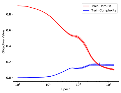
Figure 9: Complexity and data fit for GP classification on the 0-1 task.

F.3 GP Classification Complexity for Algorithmic Case

We take the same learning setting as in Section 2.1.3, showing the complexity and error curves in Figure 9 as defined in Equation 26.

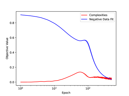
Figure 10: Complexity and data fit for GP classification on the concealed parity prediction task.

Appendix G Grokking via Concealment

G.1 Algorithm

Algorithm 1 Algorithm for relationship of $\Delta_{k}$ with dimensionality

1:$|L|>0$ $\triangleright$ Number of additional lengths

2:$|D|>0$ $\triangleright$ Number of datasets

3:$|R|>0$ $\triangleright$ Number of random seeds

4:$\gamma\leftarrow 0.95$ $\triangleright$ Threshold for high accuracy

5:$N\leftarrow 1500$ $\triangleright$ Number of epochs

6:array_of_avg, array_of_std $\leftarrow$ [], []

7:for each $l$ in $L$ do

8:     length_scale_avgs, length_scale_stds $\leftarrow$ [], []

9:     for each $d$ in $D$ do

10:         dataset_gap $\leftarrow$ []

11:         for each $r$ in $R$ do

12:              set_random_seed($r$)

13:              model $\leftarrow$ initialise_model()

14:              training_accuracy, validation_accuracy $\leftarrow$ train_model(model, $d$)

15:              training_index $\leftarrow$ first_index_above(training_accuracy, $\gamma$)

16:              validation_index $\leftarrow$ first_index_above(validation_accuracy, $\gamma$)

17:              $\Delta_{k}\leftarrow\text{{validation\_index}}-\text{{training\_index}}$

18:              dataset_gap.append($\Delta_{k}$)

19:         end for

20:         avg_gap, std_gap $\leftarrow$ avg(dataset_gap), std(dataset_gap)

21:         length_scale_avgs.append(avg_gap)

22:         length_scale_stds.append(std_gap)

23:     end for

24:     array_of_avg.append(length_scale_avgs)

25:     array_of_std.append(length_scale_stds)

26:end for

G.2 Original Regression Plot

Below we present a version of Figure 4 where we have reversed alterations to the error bars and included data from the $0$ additional length category.

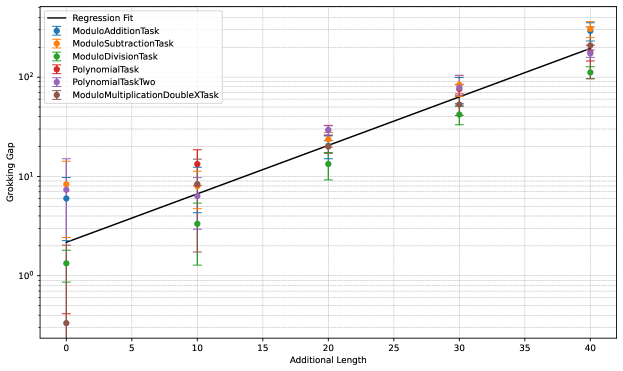
Figure 11: Relationship between grokking gap and number of additional dimensions using the grokking via concealment strategy.

Appendix H Illustrative Figures

H.1 Lengthscale Plot of GP with Parity Prediction

In Section 2.1.3, a GP is used for the hidden parity prediction task. With this dataset, models should learn to disregard dimensions with spurious data. In this case, the spurious dimensions are those above three. Presented in Figure 12 is a plot of the length scale parameter over the course of hyperparameters. As can be seen in that figure, length scale increases for for input dimensions above three but decrease for input dimensions three and below. This is expected – a larger length scale cannot discern small changes in the input dimension and thus renders them uninformative.

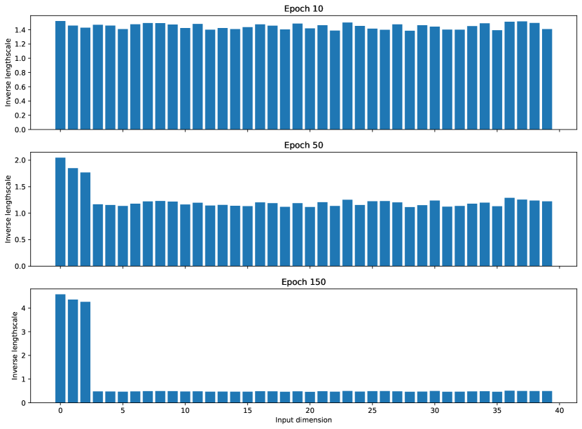
Figure 12: Example of GP kernel length scale for hidden parity prediction task. Note that inverse length scale refers to $1/l_{i}$ where $l_{i}$ is the length scale associated with dimension $i$.

H.2 Illustrative Example of Grokking

Figure 13: Illustrative example of the grokking phenomenon. The red line is the training loss and the blue line is the validation loss.

Appendix I On the complexity term in approximate inference for GP models

As shown in the main text, the exact log marginal likelihood (LML) for GP regression has interpretable terms as follows:

$$\mathcal{L}(\theta)=\log p(y|X,\theta)=-\underbrace{\frac{1}{2}y^{T}K_{\theta}^{-1}y}_{\text{data fit}}-\underbrace{\frac{1}{2}\log|K_{\theta}|}_{\text{complexity}}-\underbrace{\frac{n}{2}\log 2\pi}_{\text{normalisation}}.$$ (27)

where $K_{\theta}=K_{f}+\sigma_{n}^{2}I$. Unfortunately, the exact LML is analytically intractable for many other GP models of interest such as GP classification. In the following, we will write down the approximate LML provided by variational inference or the Laplace’s approximation. We will then look at their special case - GP regression, to identify which terms correspond to the data fit term and the complexity term in the GP regression’s LML.

I.1 Laplace approximation

Laplace’s method approximates the posterior by a Gaussian density where its mean is the mode of the posterior and its covariance is the inverse of the negative Hessian evaluated at the mode. The corresponding approximate LML is

$$\mathcal{F}_{\mathrm{Laplace}}(\theta)=-\underbrace{\frac{1}{2}{\bf\hat{f}}^{T}K_{\theta}^{-1}{\bf\hat{f}}+\log p(y|{\bf\hat{f}})}_{\text{data fit}}-\underbrace{\frac{1}{2}\log|B|}_{\text{complexity}},$$ (28)

where ${\bf\hat{f}}$ is the posterior mode, $B=I_{n}+W^{\frac{1}{2}}KW^{\frac{1}{2}}$, and $W=-\nabla\nabla\log p(y|{\bf f})$. For GP classification with a logistic likelihood function, the second derivative of the likelihood function wrt the function value does not depend on the target. That is, $B$ does not depend on y. For this reason, we can view $\frac{1}{2}\log|B|$ as a model complexity measure. To double check, when the likelihood is Gaussian as in GP regression, $B=\frac{1}{\sigma_{n}^{2}}(K_{\bf f}+\sigma_{n}^{2}I_{n})$ and hence $\frac{1}{2}\log|B|=\frac{1}{2}\log|K_{\bf f}+\sigma_{n}^{2}I_{n}|-\frac{N}{2}\log\sigma_{n}^{2}$, which is identical to the GPR’s complexity term up to a constant when the noise is fixed.

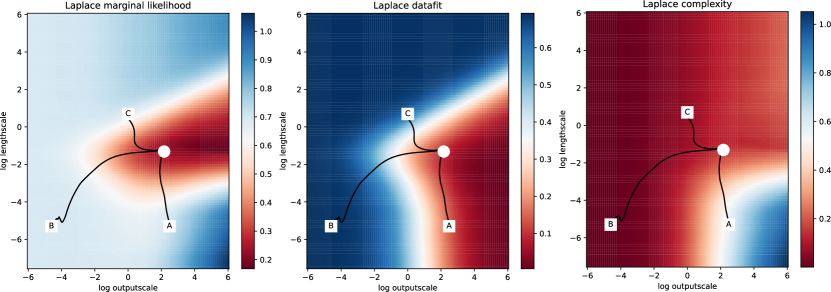
Figure 14: The approximate log marginal likelihood, data-fit and complexity provided by the Laplace’s approximation. The black curves are the trajectories of the hyperparameters with different initialisations when using variational inference.

I.2 Variational inference and the lower bound on the LML

Gaussian variational inference is widely used to perform approximate inference in GP models with non-Gaussian likelihoods such as GP classification. In this setting, the variational lower bound on the LML can be optimised to select the variational approximation and a point estimate for the model hyperparameters. Assuming $p({\bf f})=\mathcal{N}({\bf f};0,K_{\bf f})$ and $q({\bf f})=\mathcal{N}({\bf f};\mu,\Sigma)$, the variational bound can be written as follows,

$$\mathcal{F}_{\mathrm{VI}}(q({\bf f}),\theta) =\underbrace{-\mathrm{KL}(q({\bf f})||p({\bf f}))}_{\text{KL term}}+\underbrace{\int_{\bf f}q({\bf f})\log p(y|{\bf f})}_{\text{expected log likelihood}}$$ (29)

$$=-\frac{1}{2}\mu^{\intercal}K_{\bf f}^{-1}\mu-\frac{1}{2}\mathrm{trace}(K_{\bf f}^{-1}\Sigma)-\underbrace{\frac{1}{2}\log|K_{\bf f}|}_{\text{prior entropy}+\mathrm{const}}+\frac{1}{2}\log|\Sigma|-\frac{N}{2}+\int_{\bf f}q({\bf f})\log p(y|{\bf f})$$ (30)

Using the KL term as a complexity measure in this case has two connected issues:

• Unlike exact GP regression or Bayesian neural networks with a fixed prior, both the variational approximation and the hyperparameters are being optimised in variational inference. It is thus challenging to state which terms in the KL correspond to the complexity of the current fit, and which corresponds to the complexity governed by the prior model. In fact, for the GP regression case and $q({\bf f})$ is set to the exact posterior, the KL term has a data-fit component and thus does not naturally fall back to the complexity term in the GPR’s exact LML.

• One could pick the variational posterior to be the prior (which is of course a poor fit), leading to a zero KL term. However, this does not mean the complexity is zero!

Due to these potential issues, we did not see a clear relationship between the KL term and grokking in GP classification, as shown in the main text and Sections F.2 and F.3. We can work around these issues by looking at just the entropy of the prior (which resembles the complexity term in the GPR LML) or using the complexity term provided by Laplace’s method using the current hyperparameter estimates. Figure 15 shows the objective function, the learning curves and predictions made during training, for various hyperparameter initialisations. The initialisations and trajectories are shown together with the Laplace approximate LML in in Figure 14.

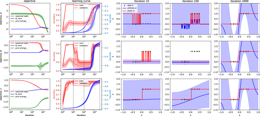
Figure 15: The objective function [first column], the learning curves [second column] and predictions made during training [final three columns], for three hyperparameter initialisations [each row corresponds to an initialisation]. A: short lengthscale and high kernel variance. B: short lengthscale and small kernel variance. C: intermediate lengthscale and kernel variance.

References

- Goodfellow et al. [2016] Ian Goodfellow, Yoshua Bengio, and Aaron Courville. Deep Learning. MIT Press, 2016.
- Burnham and Anderson [2004] Kenneth P. Burnham and David R. Anderson. Model Selection and Multimodel Inference: A Practical Information-Theoretic Approach. Springer, 2nd edition, 2004.
- Hu et al. [2021] Xia Hu, Lingyang Chu, Jian Pei, Weiqing Liu, and Jiang Bian. Model complexity of deep learning: A survey. Knowledge and Information Systems, 63:2585–2619, 2021.
- Liu et al. [2023a] Ziming Liu, Ziqian Zhong, and Max Tegmark. Grokking as compression: A nonlinear complexity perspective, 2023a.
- Yueksel et al. [2020] Hazar Yueksel, Kush R. Varshney, and Brian Kingsbury. A kolmogorov complexity approach to generalization in deep learning, 2020. URL https://openreview.net/forum?id=Bke7MANKvS.
- Hinton and van Camp [1993] Geoffrey E. Hinton and Drew van Camp. Keeping the neural networks simple by minimizing the description length of the weights. In Proceedings of the Sixth Annual Conference on Computational Learning Theory, page 5–13, 1993.
- MacKay [2003] David J. C. MacKay. Information Theory, Inference, and Learning Algorithms. Cambridge University Press, 2003.
- Rasmussen and Williams [2006] Carl Edward Rasmussen and Christopher K. I. Williams. Gaussian processes for machine learning. MIT Press, 2006.
- Bauer et al. [2016] Matthias Bauer, Mark van der Wilk, and Carl Edward Rasmussen. Understanding probabilistic sparse Gaussian process approximations. Advances in Neural Information Processing Systems, 29, 2016.
- Power et al. [2022] Alethea Power, Yuri Burda, Harri Edwards, Igor Babuschkin, and Vedant Misra. Grokking: Generalization beyond overfitting on small algorithmic datasets, 2022.
- Liu et al. [2023b] Ziming Liu, Eric J. Michaud, and Max Tegmark. Omnigrok: Grokking beyond algorithmic data. International Conference on Learning Representations, 2023b.
- Davies et al. [2023] Xander Davies, Lauro Langosco, and David Krueger. Unifying grokking and double descent, 2023.
- Barak et al. [2022] Boaz Barak, Benjamin Edelman, Surbhi Goel, Sham Kakade, Eran Malach, and Cyril Zhang. Hidden progress in deep learning: SGD learns parities near the computational limit. Advances in Neural Information Processing Systems, 35:21750–21764, 2022.
- Nanda et al. [2023] Neel Nanda, Lawrence Chan, Tom Lieberum, Jess Smith, and Jacob Steinhardt. Progress measures for grokking via mechanistic interpretability, 2023.
- Varma et al. [2023] Vikrant Varma, Rohin Shah, Zachary Kenton, János Kramár, and Ramana Kumar. Explaining grokking through circuit efficiency, 2023.
- Liu et al. [2022] Ziming Liu, Ouail Kitouni, Niklas S Nolte, Eric Michaud, Max Tegmark, and Mike Williams. Towards understanding grokking: An effective theory of representation learning. Advances in Neural Information Processing Systems, 35:34651–34663, 2022.
- Hensman et al. [2015] James Hensman, Alexander G. de G. Matthews, and Zoubin Ghahramani. Scalable variational Gaussian process classification. In Proceedings of the Eighteenth International Conference on Artificial Intelligence and Statistics, volume 38, 2015.
- Gardner et al. [2018] Jacob Gardner, Geoff Pleiss, Kilian Q Weinberger, David Bindel, and Andrew G Wilson. Gpytorch: Blackbox matrix-matrix Gaussian process inference with GPU acceleration. Advances in Neural Information Processing Systems, 31, 2018.
- Merrill et al. [2023] William Merrill, Nikolaos Tsilivis, and Aman Shukla. A tale of two circuits: Grokking as competition of sparse and dense subnetworks, 2023.
- Pearson [1895] Karl Pearson. Note on Regression and Inheritance in the Case of Two Parents. Proceedings of the Royal Society of London Series I, 58:240–242, January 1895.