CROP: Conservative Reward for Model-based Offline Policy Optimization

Abstract

Offline reinforcement learning (RL) aims to optimize policy using collected data without online interactions. Model-based approaches are particularly appealing for addressing offline RL challenges due to their capability to mitigate the limitations of offline data through data generation using models. Prior research has demonstrated that introducing conservatism into the model or Q-function during policy optimization can effectively alleviate the prevalent distribution drift problem in offline RL. However, the investigation into the impacts of conservatism in reward estimation is still lacking. This paper proposes a novel model-based offline RL algorithm, Conservative Reward for model-based Offline Policy optimization (CROP), which conservatively estimates the reward in model training. To achieve a conservative reward estimation, CROP simultaneously minimizes the estimation error and the reward of random actions. Theoretical analysis shows that this conservative reward mechanism leads to a conservative policy evaluation and helps mitigate distribution drift. Experiments on D4RL benchmarks showcase that the performance of CROP is comparable to the state-of-the-art baselines. Notably, CROP establishes an innovative connection between offline and online RL, highlighting that offline RL problems can be tackled by adopting online RL techniques to the empirical Markov decision process trained with a conservative reward. The source code is available with https://github.com/G0K0URURI/CROP.git.

Introduction

Reinforcement learning (RL) has achieved impressive performance across various many decision-making domains, including electronic games (Mnih et al. 2015), robot control (Kalashnikov et al. 2018), and recommended systems (Zhang et al. 2017). Conventional RL employs an online training paradigm where the agent optimizes policies based on real-time interactions with the environment (Sutton and Barto 2005). Online interactions can be expensive, time-consuming, or dangerous, posing a significant hurdle for widespread RL applications. To address this issue, a natural idea is to use pre-collected data instead of online interactions in RL, which is known as offline RL (Levine et al. 2020).

Directly using online RL algorithms in the offline setting often leads to extremely poor results due to the distribution shift (Kumar et al. 2020). Distribution shift arises from the difference between the behavior policy that produced the offline data and the learned policy, which may cause erroneous overestimation of Q-function and damage the performance. To alleviate the distribution drift, many model-free offline RL algorithms incorporate conservatism or regularization to constrain the learned policy (Kumar et al. 2020; Cheng et al. 2022; Kumar et al. 2019; Kostrikov et al. 2021; Shi et al. 2022). However, model-free algorithms can only directly learn about the states in the offline data and cannot generalize environmental information, which may lead to myopia and poor performance in unseen states.

Model-based offline RL algorithms solve the limitation by training a environment model for interactions with the agent. Nevertheless, distribution drift can also negatively impact model-based offline RL methods. The model accuracy inherently diminishes for state-action pairs that lie beyond the scope of the offline dataset. These inaccurate situations may be accessed by the agent due to the distribution drift and affect the effect of policy optimization. Several methods use uncertainty estimation to penalize the situations with low model accuracy. However, these methods rely on some sort of strong heuristic assumption about uncertainty estimation (Yu et al. 2020; Sun et al. 2023) or directly detect out-of-distribution (OOD) state-action tuples (Kidambi et al. 2020), which might prove fragile or impractical in complex environments. Furthermore, some researchers have heuristically designed elaborate structures, such as introducing counters(Kim and Oh 2023) or inverse dynamic functions (Lyu, Li, and Lu 2022), to punish OOD data. To eschew uncertainty estimation or other addition parts, several methods induce conservatism into the model (Rigter, Lacerda, and Hawes 2022; Bhardwaj et al. 2023) or Q-function (Yu et al. 2021) in policy optimization and underestimate OOD state-action tuples, indirectly mitigating distribution shift (Yu et al. 2021; Rigter, Lacerda, and Hawes 2022; Bhardwaj et al. 2023).

The main contributions of this paper are as follows:

• A novel model-based offline RL algorithm, Conservative Reward for model-based Offline Policy optimization (CROP), is proposed in this paper. The proposed method conservatively estimates the reward in model training by minimizing rewards of random actions alongside the estimation error, then uses the existing online RL method in policy optimization. This provides a new perspective bridging offline and online RL, where offline RL can be solved by online RL methods in the empirical MDP with the conservative reward.

• Theoretical analysis gives a lower bound on the performance of CROP and demonstrates that the proposed method CROP is capable of underestimating Q-function and mitigating distribution drift.

• Experimental results show that CROP obtains the state-of-the-art results on D4RL benchmark tasks.

Related Work

In offline RL, there is no opportunity of improving exploration during policy optimization. When offline data sufficiently cover the state-action space, online RL methods can perform well without additional modification  (Agarwal, Schuurmans, and Norouzi 2019). However, in more common cases offline data is insufficiently covered. Using out-of-distribution (OOD) actions is necessary to find better policies, but also brings potential risks, which need to be balanced in policy optimization (Levine et al. 2020). Online RL methods often perform extremely poorly in such settings due to overestimation caused by the distribution shift (Fu et al. 2020; Kumar et al. 2020). Below, we discuss how existing offline methods address this challenge.

Model-free offline RL: Existing model-free offline RL methods can be broadly categorized into policy constraint and value regularization. Policy constraint methods introduce constraints based on the behavior policy, directly restricting the learned policy to be close to the behavior policy (Fujimoto, Meger, and Precup 2019; Fujimoto and Gu 2021; Ghasemipour, Schuurmans, and Gu 2021) or avoiding OOD actions in Bellman backup operator (Kumar et al. 2019). These methods directly limit the scope of policy optimization and may perform poorly when the behavioral policy is inferior. In contrast, value regularization methods avoid OOD actions indirectly by underestimating the value function. Value regularization can be achieved by conservatively estimating value function (Kumar et al. 2020; Cheng et al. 2022; Lyu et al. 2022), or penalizing uncertainty based on Q function ensembles (An et al. 2021; Bai et al. 2022).

Model-based offline RL: Model-based offline RL methods first train an environment model based on the offline data, then utilize interactions with the trained models to extend the offline data. A major approach to eliminating distribution drift in offline RL is to penalize model uncertainty (Yu et al. 2020; Sun et al. 2023; Lu et al. 2022; Rafailov et al. 2021). However, methods that rely on model uncertainty often necessitate strong prior assumptions during uncertainty quantification. For example, MOPO and MOBILE respectively assume variance and Bellman inconsistency as reasonable estimates of model uncertainty. These assumptions may not hold in specific cases. To avoid model uncertainty estimators, additional parts, such as counters and discriminators, are incorporated into the model to conservatively estimate OOD action (Kim and Oh 2023; Kidambi et al. 2020; Lyu, Li, and Lu 2022). Moreover, some research directly introduces conservatism into the model or Q-function and designs offline RL methods without additional parts or model uncertainty (Yu et al. 2021; Rigter, Lacerda, and Hawes 2022; Bhardwaj et al. 2023).

The proposed method CROP is similar to the existing methods COMBO (Yu et al. 2021), RAMBO (Rigter, Lacerda, and Hawes 2022), and ARMOR (Bhardwaj et al. 2023), all of which incorporate conservatism into the fundamental components of model-based RL (the model or Q-function) to avoid overestimation. Compared with the existing three methods, CROP is mainly different in two places:

• While the existing three methods introduce conservatism in the Q-function or the entire model, CROP only introduces conservatism in the model’s reward estimate.

• CROP conservatively estimates rewards during model training, whereas these methods achieve conservatism during policy optimization. Since the number of steps required for model training is empirically much smaller than that required for policy optimization, CROP can compute and back-propagate conservative losses less often. Furthermore, CROP directly adopts online RL methods during policy optimization, providing a new perspective on bridging offline and online RL that offline RL can be solved by applying online RL methods on the empirical MDP with conservative rewards.

Preliminaries

Reinforcement learning (RL) is used for optimization problems in Markov decision processes (MDP). An MDP is defined by a tuple $\left(\mathcal{S},\mathcal{A},T,R,\mu_{0},\gamma\right)$, where $\mathcal{S}$ and $\mathcal{A}$ represent the state and action spaces. $T$, $R$, $\mu_{0}$, and $\gamma$ denote the transition probability, reward, initial state distribution, and discount factor, respectively. At time step $t$ with state $s\in\mathcal{S}$, the agent chooses an action $a$ based on a policy $\pi(a|s)$. Then the state changes from $s$ to $s^{\prime}$ based on the transition probability $T(s^{\prime}|s,a)$, and the agent obtains a reward $R(s,a)\in\left[-R_{\max},R_{\max}\right]$. The goal of RL is to find the optimal policy that maximizes the expected cumulative discounted reward $\sum_{t}\mathbb{E}_{s,a}\left[\gamma^{t}R(s,a)\right]$ in the MDP. Offline RL is a special formulation of RL that only uses previously collected datasets $\mathcal{D}=\left\{(s,a,R(s,a),s^{\prime})\right\}$ during training (Levine et al. 2020). We use $\bar{\pi}$ to denote the empirical behavior policy in $\mathcal{D}$.

Method

Algorithm 1 Conservative Reward for model-based Offline Policy optimization (CROP)

1:offline data $\mathcal{D}=\left\{(s,a,R(s,a),s^{\prime})\right\}$

2:loop$\triangleright$ model training

3:     divide $\mathcal{D}$ into a train set and a valid set;

4:     loop

5:         train $\hat{T}$ using Equation 1;

6:     end loop

7:     loop

8:         train $\hat{r}$ using Equation 2;

9:     end loop

10:end loop

11:recompute the reward in $\mathcal{D}$;

12:loop$\triangleright$ policy optimization

13:     interact with the model using policy $\pi$;

14:     update Q-function $\hat{Q}^{\pi}$ using Equation 4

15:     update policy $\pi$ using Equation 6

16:     update $\alpha$ using Eqation 7

17:     update the target Q-function $Q_{\mathrm{tar}}$

18:end loop

19:the learned policy $\pi$

Model training with conservative reward estimation

The proposed algorithm, Conservative Reward for model-based Offline Policy optimization (CROP), aims to integrate the conservative evaluation of out-of-distribution (OOD) actions in the process of model training, to avoid additional consideration of avoiding OOD actions and directly utilize existing online RL algorithms in policy optimization.

The model consists of a transition probability estimator $\hat{T}$ and a reward estimator $\hat{r}$. In the model training, the transition probability estimator $\hat{T}$ is updated by maximizing log-probability:

$$l_{T}=\mathbb{E}_{\mathcal{D}}\left\{-\log\hat{T}(s^{\prime}|s,a)\right\}.$$ (1)

The reward estimator $\hat{r}$ should minimize the estimation error as well as underestimate actions outside $\mathcal{D}$ as much as possible, which is achieved by the following loss:

$$l_{r}=\mathbb{E}_{\mathcal{D}}\left\{\left[\hat{r}(s,a)-R(s,a)\right]^{2}+\beta\hat{r}(s,\bar{a})\right\},$$ (2)

where $\bar{a}$ denotes random actions and hyperparameter $\beta$ controls the underestimation. By setting the derivative of Equation 2 to zero, we obtain the optimal conservative reward estimation $r$:

$$r\left(s,a\right)=R\left(s,a\right)-\beta\frac{\mu}{\bar{\pi}(a|s)},$$ (3)

where $\mu$ is the probability density of a uniform distribution in the action space $\mathcal{A}$, and $\bar{\pi}$ is the behavior policy of $\mathcal{D}$. The second term on RHS of Equation 3 represents the conservativeness of the reward estimation, which is inversely proportional to the probability of the action appearing in $\mathcal{D}$.

By interacting with models that use the conservative reward estimation, online RL algorithms can avoid OOD actions and improve policies safely for offline RL problems, which will be shown in Section Theoretical analysis of CROP. Therefore, CROP provides a new perspective to connect offline and online RL that offline RL can be regarded as online RL under conservative reward estimation, which helps to apply the appealing development of online RL to offline RL.

Practical implementation

Now we describe a practical implementation of CROP using the conservative reward estimation above. The algorithm is summarized in Algorithm 1, which consists of model training and policy optimization.

In model training, we learn an ensemble of models, and each model is trained independently. For each model, the offline data $\mathcal{D}$ is divided into a train set and a valid set, and then $\hat{T}$ and $\hat{r}$ are trained using Function 1 and Function 2, respectively.

After model training, the reward in offline data $R_{t}$ is replaced by the mean of $\hat{r}$. Then an online model-free RL algorithm, Soft Actor-Critic (SAC) (Haarnoja et al. 2018), is used to optimize the policy from offline data and online interactions with the model ensemble. In interactions with the model ensemble, the reward is computed as the mean of $\hat{r}$, while the next state is the output of $\hat{T}$ in a model chosen at random. The initial state of the interaction is randomly sampled from the offline data $\mathcal{D}$, and the interaction lasts for $k$ steps. In each step of policy optimization, a mini-batch data $\mathcal{D}_{f}$ is sampled, where the proportion of online interaction data is $f$. Q-function of policy $\pi$, which is denoted by $\hat{Q}^{\pi}$, is trained by minimizing the soft Bellman residual

$$l_{\hat{Q}^{\pi}}=\mathbb{E}_{\mathcal{D}_{f}}\{[\hat{Q}^{\pi}\left(s,a\right)-\hat{r}\left(s,a\right)-\gamma\hat{V}^{\pi}\left(s^{\prime}\right)]^{2}\}.$$ (4)

$V$ is estimated by Monte Carlo method

$$\hat{V}^{\pi}(s)=\mathbb{E}_{a\sim\pi(\cdot|s)}[Q_{\mathrm{tar}}(s,a)-\alpha\log\pi(a|s)],$$ (5)

where the target Q-function $Q_{\mathrm{tar}}$ is an exponentially moving average of $\hat{Q}^{\pi}$. The policy $\pi$ is trained by maximizing value function $V^{\pi}$ and keeping a reasonable entropy with a Lagrangian relaxation. The policy loss function $l_{\pi}$ is as follows:

$$l_{\pi}=\mathbb{E}_{\mathcal{D}_{f}}\left\{\alpha\mathcal{H}[\pi(\cdot|s)]-\hat{V}^{\pi}(s)\right\},$$ (6)

where $\mathcal{H}(\cdot)$ stands for entropy. $\alpha$ is a non-negative parameter updated by minimizing the following loss function:

$$l_{\alpha}=\mathbb{E}_{\mathcal{D}_{f}}\left\{\alpha\mathcal{H}[\pi(\cdot|s)]-\alpha\bar{\mathcal{H}}\right\},$$ (7)

where hyperparameter $\bar{\mathcal{H}}$ is the target entropy.

$\hat{T}$, $\hat{r}$, $Q_{\rm{tar}}$, $\hat{Q}^{\pi}$ and $\pi$ are all parameterized with multi-layer perceptrons.

Theoretical analysis of CROP

In the following, we theoretically analyze the proposed method CROP and show that it underestimates Q-function and satisfies safe policy improvement guarantees. In the following we discuss the tabular case, and the proof on the continuous case is similar and omitted for brevity.

Let $\bar{T}$ and $\bar{r}$ denote the empirical transition probability and the empirical conservative reward, which are the optimal estimations of $T$ and $r$ from $\mathcal{D}$. The difference between $(\bar{T},\bar{r})$ and $(T,r)$ comes from the sample bias during offline data collection, while the difference between $(\bar{T},\bar{r})$ and $(\hat{T},\hat{r})$ comes from the estimation error of models (neural networks in this paper). The sample bias and the estimation error are the main factors affecting the performance of the algorithm. To express the Q-function update conveniently, we use $B^{T,r,\pi}$ to denote the Bellman operator about policy $\pi$ in the MDP with transition probability $T$ and reward $r$:

$$B^{T,r,\pi}Q^{\pi}=r+\gamma T^{\pi}Q^{\pi},$$ (8)

where $T^{\pi}$ denotes the state transition probability with policy $\pi$: $T^{\pi}(s^{\prime}|s)=\sum_{a}\pi(a|s)T(s^{\prime}|s,a)$. Following the standard assumption in model-based offline RL literature (Yu et al. 2021; Laroche, Trichelair, and des Combes 2019), we assume that the sample bias and the estimation error are bounded as following:

Assumption 1.

$\forall s,a\in D$, the following relationships hold

$$\begin{split}|\bar{r}\left(s,a\right)-r\left(s,a\right)|\leq\frac{C_{r}}{\sqrt{|D\left(s,a\right)|}},\\ ||\bar{T}\left(s^{\prime}|s,a\right)-T\left(s^{\prime}|s,a\right)||_{1}\leq\frac{C_{T}}{\sqrt{|D\left(s,a\right)|}},\end{split}$$ (9)

Assumption 2.

$\forall s,a\in D$, the model estimation bias is bounded:

$$|\hat{r}\left(s,a\right)-\bar{r}\left(s,a\right)|\leq\epsilon_{r},||\hat{T}\left(s^{\prime}|s,a\right)-\bar{T}\left(s^{\prime}|s,a\right)||_{1}\leq\epsilon_{T}$$ (10)

Firstly, We state that the Q-function $\hat{Q}^{\pi}$ in CROP conservatively estimates the true Q-function:

Proposition 1.

For large enough $\beta$, we have

$$\mathbb{E}_{s\sim\mu_{0},a\sim\pi(\cdot|s)}\left[\hat{Q}^{\pi}(s,a)\right]\leq\mathbb{E}_{s\sim\mu_{0},a\sim\pi(\cdot|s)}\left[Q^{\pi}(s,a)\right],$$ (11)

where $Q^{\pi}$ is the Q-function of $\pi$ in the actual MDP, i.e. the fixed point of $B^{T,R,\pi}$, and $\mu_{0}$ is the initial state distribution.

Proof.

With Assumption 1, the difference between $B^{\bar{T},\bar{r},\pi}$ and $B^{T,r,\pi}$ can be bounded:

$$\left|B^{T,r,\pi}Q^{\pi}\left(*\right)-B^{\bar{T},\bar{r},\pi}Q^{\pi}\left(*\right)\right|$$ (12)

$$=\left|(r\left(*\right)-\bar{r}\left(*\right))+\gamma\sum_{s^{\prime}}\left(T\left(s^{\prime}|*\right)-\bar{T}\left(s^{\prime}|*\right)\right)V^{\pi}(s^{\prime})\right|$$

$$\leq\left|(r\left(*\right)-\bar{r}\left(*\right))\right|+\gamma\left|\sum_{s^{\prime}}\left(T\left(s^{\prime}|*\right)-\bar{T}\left(s^{\prime}|*\right)\right)V^{\pi}(s^{\prime})\right|$$

$$\leq\frac{C_{r}+\gamma C_{T}2R_{\max}/(1-\gamma)}{\sqrt{|D\left(*\right)|}},$$

where $*$ denotes $(s,a)$ and $V^{\pi}(s)=\sum_{a}\pi(a|s)Q(a|s)$. This gives us an expression, which is a function of $C_{r}$ and $C_{P}$, to bound the potential overestimation caused by the sample bias.

In the proposed algorithm, only state transitions of offline date are kept, and the reward for offline data is replaced by the reward of environment model. Thus, the Bellman operator using offline data is $B^{\bar{T},\hat{r},\pi}$, whose difference to $B^{\bar{T},\bar{r},\pi}$ is bounded by $\epsilon_{r}$:

$$\begin{split}\left|B^{\bar{T},\hat{r},\pi}Q^{\pi}\left(*\right)-B^{\bar{T},\bar{r},\pi}Q^{\pi}\left(*\right)\right|=|\hat{r}\left(*\right)-\bar{r}\left(*\right)|\leq\epsilon_{r}.\end{split}$$ (13)

The Bellman operator using interactions with the model is $B^{\hat{T},\hat{r},\pi}$, whose difference to $B^{\bar{T},\bar{r},\pi}$ is bounded as follows:

$$\left|B^{\hat{T},\hat{r},\pi}Q\left(*\right)-B^{\bar{T},\bar{r},\pi}Q\left(*\right)\right|$$ (14)

$$=\left|\hat{r}\left(*\right)-\bar{r}\left(*\right)+\gamma\sum_{s^{\prime}}\left(\hat{T}\left(s^{\prime}|*\right)-\bar{T}\left(s^{\prime}|*\right)\right)V^{\pi}(s^{\prime})\right|$$

$$\leq\left|\hat{r}\left(*\right)-\bar{r}\left(*\right)\right|+\left|\gamma\sum_{s^{\prime}}\left(\hat{T}\left(s^{\prime}|*\right)-\bar{T}\left(s^{\prime}|*\right)\right)V^{\pi}(s^{\prime})\right|$$

$$\leq\epsilon_{r}+\gamma\epsilon_{P}2R_{\max}/(1-\gamma).$$

Since offline data and interactions with the model are mixed in the ratio $(1-f):f$ for policy optimization in CROP, the Bellman operator used in CROP $B_{\rm{CROP}}$ can be seen as a mix of $B^{\bar{T},\hat{r},\pi}$ and $B^{\hat{T},\hat{r},\pi}$:

$$B_{\rm{CROP}}Q\left(*\right)=\left[(1-f)B^{\bar{T},\hat{r},\pi}+fB^{\hat{T},\hat{r},\pi}\right]Q\left(*\right)$$ (15)

$$\leq B^{T,r,\pi}Q\left(*\right)+\left|B^{T,r,\pi}Q\left(*\right)-B^{\bar{T},\bar{r},\pi}Q\left(*\right)\right|$$

$$+(1-f)\left|B^{\bar{T},\hat{r},\pi}Q\left(*\right)-B^{\bar{T},\bar{r},\pi}Q\left(*\right)\right|$$

$$+f\left|B^{\hat{T},\hat{r},\pi}Q\left(*\right)-B^{\bar{T},\bar{r},\pi}Q\left(*\right)\right|$$

$$\leq B^{T,r,\pi}Q\left(*\right)+\frac{C_{r}+\gamma C_{T}2R_{\max}/(1-\gamma)}{\sqrt{|D\left(*\right)|}}$$

$$+(1-f)\epsilon_{r}+f\left(\epsilon_{r}+\gamma\epsilon_{T}2R_{\max}/\left(1-\gamma\right)\right)$$

$$=B^{T,R,\pi}Q\left(*\right)-\beta\frac{\mu}{\bar{\pi}(a|s)}+\frac{C_{r}+\gamma C_{T}2R_{\max}/(1-\gamma)}{\sqrt{|D\left(*\right)|}}$$

$$+\epsilon_{r}+f\gamma\epsilon_{T}2R_{\max}/\left(1-\gamma\right).$$

$\hat{Q}^{\pi}(*)$ is the fixed point of $B_{\rm{CROP}}$, and $Q^{\pi}\left(*\right)$ is the fixed point of $B^{P,R,\pi}$. Define the terms independent of $\beta$ in the RHS of Equation 15 as $\phi$: $\phi=\frac{C_{r}+\gamma C_{T}2R_{\max}/(1-\gamma)}{\sqrt{|D\left(s,a\right)|}}+\epsilon_{r}+f*\gamma\epsilon_{T}2R_{\max}/\left(1-\gamma\right)$. By computing the fixed point of equation 15, $\hat{Q}^{\pi}(*)$ can be bounded as follows:

$$\hat{Q}^{\pi}(*)\leq Q^{\pi}\left(*\right)-\beta*\left[S^{\pi}\frac{\mu}{\bar{\pi}}\right]\left(*\right)+\left[S^{\pi}\phi\right]\left(*\right),$$ (16)

where $S^{\pi}=\left(I-\gamma T^{\pi}\right)^{-1}$.

Thus, by choosing large enough $\beta$, $\hat{Q}^{\pi}(*)\leq Q^{\pi}\left(*\right)$ and $\mathbb{E}_{s\sim\mu_{0},a\sim\pi(\cdot|s)}\left[\hat{Q}^{\pi}(s,a)\right]\leq\mathbb{E}_{s\sim\mu_{0},a\sim\pi(\cdot|s)}\left[Q^{\pi}(s,a)\right]$. ∎

Proposition 1 shows that CROP can conservatively estimate Q-function and avoid the common overestimation problem in offline RL. However, not all conservative estimations help avoid OOD actions. As an extreme example, for all bounded $\hat{Q}^{\pi}$, there always exists a constant large enough that $\hat{Q}^{\pi}(*)$ minus the constant is smaller than $Q^{\pi}(*)$. However, this constant subtraction on Q-function does not change the relative merits of actions and has no effect on policy optimization. Thus, it is necessary to prove that CROP is effective in avoiding OOD actions.

Proposition 2.

$\forall a_{1},a_{2}\in A,s_{1},s_{2}\in S$, if $\bar{\pi}\left(a_{1}|s_{1}\right)<\bar{\pi}\left(a_{2}|s_{2}\right)$, for large enough $\beta$,

$$Q^{\pi}\left(s_{1},a_{1}\right)-\hat{Q}^{\pi}(s_{1},a_{1})>Q^{\pi}\left(s_{2},a_{2}\right)-\hat{Q}^{\pi}(s_{2},a_{2}).$$ (17)

Proof.

Similar to equation 15,

$$B_{\rm{CROP}}Q^{\pi}\left(*\right)=\left[(1-f)B^{\bar{P},\hat{r},\pi}+fB^{\hat{P},\hat{r},\pi}\right]Q^{\pi}\left(*\right)$$ (18)

$$\geq B^{P,r,\pi}Q^{\pi}\left(*\right)-\left|B^{P,r,\pi}Q^{\pi}\left(*\right)-B^{\bar{P},\bar{r},\pi}Q^{\pi}\left(*\right)\right|$$

$$-(1-f)\left|B^{\bar{P},\hat{r},\pi}Q^{\pi}\left(*\right)-B^{\bar{P},\bar{r},\pi}Q^{\pi}\left(*\right)\right|$$

$$-f\left|B^{\hat{P},\hat{r},\pi}Q^{\pi}\left(*\right)-B^{\bar{P},\bar{r},\pi}Q^{\pi}\left(*\right)\right|$$

$$\geq B^{P,R,\pi}Q^{\pi}\left(*\right)-\beta\frac{\mu}{\bar{\pi}(a|s)}-\phi.$$

Computing the fixed points on both sides of equation 18 yields the following:

$$\hat{Q}^{\pi}(*)\geq Q^{\pi}\left(*\right)-\beta*\left[S^{\pi}\frac{\mu}{\bar{\pi}}\right]\left(*\right)-\left[S^{\pi}\phi\right]\left(*\right)$$ (19)

Therefore,

$$\left(Q^{\pi}\left(s_{1},a_{1}\right)-\hat{Q}^{\pi}(s_{1},a_{1})\right)-\left(Q^{\pi}\left(s_{2},a_{2}\right)-\hat{Q}^{\pi}(s_{2},a_{2})\right)\geq$$ (20)

$$\beta*\left\{\left[S^{\pi}\frac{\mu}{\bar{\pi}}\right]\left(s_{1},a_{1}\right)-\left[S^{\pi}\frac{\mu}{\bar{\pi}}\right]\left(s_{2},a_{2}\right)\right\}$$

$$-\left[S^{\pi}\phi\right]\left(s_{1},a_{1}\right)-\left[S^{\pi}\phi\right]\left(s_{2},a_{2}\right)$$

For large enough $\beta$, $\left(Q^{\pi}\left(s_{1},a_{1}\right)-\hat{Q}^{\pi}(s_{1},a_{1})\right)-\left(Q^{\pi}\left(s_{2},a_{2}\right)-\hat{Q}^{\pi}(s_{2},a_{2})\right)>0$, i.e., $Q^{\pi}\left(s_{1},a_{1}\right)-\hat{Q}^{\pi}(s_{1},a_{1})>Q^{\pi}\left(s_{2},a_{2}\right)-\hat{Q}^{\pi}(s_{2},a_{2})$ ∎

Proposition 2 states that with suitable hyperparameters, the conservatism ($Q^{\pi}$ minus $\hat{Q}^{\pi}$) in CROP is stronger for actions that occur less frequently in $\bar{\pi}$, thus avoiding OOD actions in policy optimization. When $\beta$ comes to $+\infty$, $\arg\max_{a}\hat{Q}^{\pi}(\cdot|s)=\arg\max_{a}\bar{\pi}(\cdot,s)$, and the optimal policy in CROP $\pi^{*}$ directly chooses the most likely action in $\bar{\pi}$.

Hyperparameter	Value
Hidden units of model	200
Hidden units of policy	256
Number of layers in model	4
Number of layers in Q-function	2
Number of layers in policy	2
Ratio of valid set in $\mathcal{D}$	0.01
Nonlinear activation	ReLU
Batch size in model training	256
Batch size in policy optimization	512
$f$	0.5
Optimizer	Adam
Learning rate of model	1e-3
Learning rate of Q-function	3e-4
Learning rate of policy	1e-4
Learning rate of alpha	3e-5
Discount factor $\gamma$	0.99
Exponentially moving average of $\bar{Q}$	0.005
Replay buffer size for model-generated data	10000

Table 1: Value of Hyperparameters

The core evaluation metric for offline RL algorithms is the performance of the learned policy. The proposed algorithm CROP has a safe policy improvement guarantee as stated in the following.

Proposition 3.

The optimal policy $\pi^{*}$ learned by maximizing $\hat{Q}^{\pi}$

$$\pi^{*}=\arg\max_{\pi}\mathbb{E}_{s\sim\mu_{0},a\sim\pi(\cdot|s)}\left[\hat{Q}^{\pi}(s,a)\right]$$ (21)

is performed not worse than the behavior policy $\bar{\pi}$ with toleration $\delta$:

$$\mathbb{E}_{s\sim\mu_{0},a\sim\pi^{*}(\cdot|s)}\left[Q^{\pi^{*}}(s,a)\right]\geq\mathbb{E}_{s\sim\mu_{0},a\sim\bar{\pi}(\cdot|s)}\left[Q^{\bar{\pi}}(s,a)\right]-\delta.$$ (22)

$\delta$ is a function about the sample bias, estimation errors, and difference between $\pi^{*}$ and $\bar{\pi}$, which is detailed in the proof ($\delta$-safe policy improvement).

Proof.

For ease of writing, we define the expected cumulative reward of policy $\pi$ in a MDP with transition probability $T$ and reward $r$ as $F(T,r,\pi)=\mathbb{E}_{s\sim\mu_{0},a\sim\pi(\cdot|s)}\left[Q^{\pi}(s,a)\right]$. Similarly define $F(\bar{T},\bar{r},\pi)=\mathbb{E}_{s\sim\mu_{0},a\sim\pi(\cdot|s)}\left[\bar{Q}^{\pi}(s,a)\right]$ and $F(T_{f},\hat{r},\pi)=\mathbb{E}_{s\sim\mu_{0},a\sim\pi(\cdot|s)}\left[\hat{Q}^{\pi}(s,a)\right]$, where $T_{f}=(1-f)\bar{T}+f\hat{T}$

Step 1: Relate $F(T_{f},R,\pi^{*})$ and $F(T_{f},R,\bar{\pi})$. Since $\pi^{*}$ optimizes Equation 21,

$$F(T_{f},\hat{r},\pi^{*})\geq F(T_{f},\hat{r},\bar{\pi}).$$ (23)

Since $\left|\bar{r}-\hat{r}\right|\leq\epsilon_{r}$,

$$F(T_{f},R-\beta\frac{\mu}{\bar{\pi}(a|s)}+\frac{C_{r}}{\sqrt{|D\left(s,a\right)|}}+\epsilon_{r},\pi^{*})$$ (24)

$$\geq F(T_{f},R-\beta\frac{\mu}{\bar{\pi}(a|s)}-\frac{C_{r}}{\sqrt{|D\left(s,a\right)|}}-\epsilon_{r},\bar{\pi}).$$

Arranging Equation 24 can get:

$$F(T_{f},R,\pi^{*})\geq F(T_{f},R,\bar{\pi})+F(T_{f},\beta\frac{\mu}{\bar{\pi}(a|s)},\pi^{*})$$ (25)

$$-\beta-\frac{2\epsilon_{r}}{1-\gamma}-F(T_{f},\frac{C_{r}}{\sqrt{|D\left(s,a\right)|}},\pi^{*})$$

$$-F(T_{f},\frac{C_{r}}{\sqrt{|D\left(s,a\right)|}},\bar{\pi}).$$

$$F(T_{f},\frac{C_{r,\delta}}{\sqrt{|D\left(s,a\right)|}},\pi)=\sum_{s}\sum_{a}\frac{C_{r}\pi(a|s)d^{\pi}_{T_{f}}(s)}{\sqrt{|D\left(s\right)|\bar{\pi}(a|s)}}$$ (26)

$$=\sum_{s}\frac{C_{r,\delta}d^{\pi}_{T_{f}}(s)}{\sqrt{|D\left(s\right)|}}\sum_{a}\frac{\pi(a|s)}{\sqrt{\bar{\pi}(a|s)}}$$

$$\leq\sum_{s}\frac{C_{r,\delta}d^{\pi}_{T_{f}}(s)}{\sqrt{|D\left(s\right)|}}\sqrt{|A|\left[D_{\rm{CQL}}(\pi,\bar{\pi})(s)+1\right]}.$$

where $d^{\pi}_{T_{f}}$ is the distribution of state with the transition probility $T_{f}$ and policy $\pi$. $D_{\rm{CQL}}(\pi,\bar{\pi})(s)=\sum_{a}\pi(a|s)\left(\frac{\pi(a|s)}{\bar{\pi}(a|s)}-1\right)$ is defined as in (Kumar et al. 2020) and can be bounded as:

$$D_{\rm{CQL}}(\pi,\bar{\pi})(s)+1\leq(\sum_{a}\frac{\pi(a|s)}{\sqrt{\bar{\pi}(a|s)}})^{2},$$ (27)

$$|A|\left[D_{\rm{CQL}}(\pi,\bar{\pi})(s)+1\right]\geq(\sum_{a}\frac{\pi(a|s)}{\sqrt{\bar{\pi}(a|s)}})^{2}.$$

$$F(T_{f},\beta\frac{\mu}{\bar{\pi}(a|s)},\pi)=\sum_{s}\sum_{a}\beta\frac{\mu}{\bar{\pi}(a|s)}\pi(a|s)d^{\pi}_{T_{f}}(s)$$ (28)

$$=\sum_{s}\beta d^{\pi}_{T_{f}}(s)\sum_{a}\frac{\pi(a|s)}{\sqrt{\bar{\pi}(a|s)}}\frac{\mu}{\sqrt{\bar{\pi}(a|s)}}$$

$$\geq\sum_{s}\beta d^{\pi}_{T_{f}}(s)\sqrt{D_{\rm{CQL}}(\pi,\bar{\pi})(s)+1}\sqrt{D_{\rm{CQL}}(\pi_{\rm{ran}},\bar{\pi})(s)+1},$$

where $\pi_{\rm{ran}}$ is the random policy and $\pi_{\rm{ran}}(s,a)=\mu$ for all $(s,a)$.

Therefore,

$$F(T_{f},R,\pi^{*})\geq F(T_{f},R,\bar{\pi})-\Delta_{R},$$ (29)

where

$$\Delta_{R}=\sum_{s}\frac{C_{r,\delta}}{\sqrt{|D\left(s\right)|}}\left\{d^{\pi^{*}}_{T_{f}}(s)\sqrt{|A|\left[D_{\rm{CQL}}(\pi^{*},\bar{\pi})(s)+1\right]}\right.$$ (30)

$$\left.+d^{\bar{\pi}}_{T_{f}}(s)\sqrt{|A|}\right\}+\beta+\frac{2\epsilon_{r}}{1-\gamma}$$

$$-\sum_{s}\beta d^{\pi}_{T_{f}}(s)\sqrt{D_{\rm{CQL}}(\pi,\bar{\pi})(s)+1}\sqrt{D_{\rm{CQL}}(\pi_{\rm{ran}},\bar{\pi})(s)+1}$$

Step 2: Relate $F(T_{f},R,\cdot)$ and $F(T,R,\cdot)$.

$$F(T_{f},R,\pi) =F(T,R,\pi)$$ (31)

$$+\frac{\gamma}{1-\gamma}\mathbb{E}_{s,a\sim d_{T_{f}}^{\pi}(s)\pi(a|s)}\left[(T_{f}^{\pi}-T^{\pi})Q^{\pi}\right]$$

The above equation comes from Simulation Lemma (Chapter 2, Lemma 2.2) in (Agarwal, Jiang, and Kakade 2019). Therefore,

$$|F(T_{f},R,\pi)-F(T,R,\pi)|$$ (32)

$$\leq\frac{\gamma R_{\max}}{(1-\gamma)^{2}}\mathbb{E}_{s,a\sim d_{T_{f}}^{\pi}(s)\pi(a|s)}\left[||T_{f}^{\pi}-T^{\pi}||_{1}\right]$$

$$\leq\frac{\gamma R_{\max}}{(1-\gamma)^{2}}\left\{\mathbb{E}_{s,a\sim d_{T_{f}}^{\pi}(s)\pi(a|s)}\left[||\bar{T}^{\pi}-T^{\pi}||_{1}\right]+f\epsilon_{P}\right\}$$

$$\mathbb{E}_{s,a\sim d_{T_{f}}^{\pi}(s)\pi(a|s)}\left[||\bar{T}^{\pi}-T^{\pi}||_{1}\right]$$ (33)

$$=\sum_{s}\sum_{a}||\bar{T}(\cdot|s,a)-T(\cdot|s,a)||_{1}\pi(a|s)d^{\pi}_{T_{f}}(s)$$

$$\leq\sum_{s}\sum_{a}\frac{C_{T}}{\sqrt{|D\left(s,a\right)|}}\pi(a|s)d^{\pi}_{T_{f}}(s)$$

$$=\sum_{s}\frac{C_{T}d^{\pi}_{T_{f}}(s)}{\sqrt{|D\left(s\right)|}}\sum_{a}\frac{\pi(a|s)}{\sqrt{\bar{\pi}(a|s)}}$$

$$\leq\sum_{s}\frac{C_{T}d^{\pi}_{T_{f}}(s)}{\sqrt{|D\left(s\right)|}}\sqrt{|A|\left[D_{\rm{CQL}}(\pi,\bar{\pi})(s)+1\right]}$$

$$|F(P_{f},R,\pi)-F(P,R,\pi)|\leq\Delta_{P}(\pi)=$$ (34)

$$\frac{\gamma R_{\max}}{(1-\gamma)^{2}}\left\{f\epsilon_{P}+\sum_{s}\frac{C_{T}d^{\pi}_{T_{f}}(s)}{\sqrt{|D\left(s\right)|}}\sqrt{|A|\left[D_{\rm{CQL}}(\pi,\bar{\pi})(s)+1\right]}\right\}$$

Step 3: Relate $F(P,R,\pi^{*})$ and $F(P,R,\bar{\pi})$. Combining step 1 and step 2,

$$F(P,R,\pi^{*})\geq F(P,R,\bar{\pi})-\delta,$$ (35)

where $\delta=\Delta_{R}+\Delta_{P}(\pi^{*})+\Delta_{P}(\bar{\pi})$. ∎

Experiment

Conservative reward visualization

To visualize the proposed conservative reward, we design a simple 1-dimension MDP where the state is always 0 and the action space is $[-1,1]$. The reward $R$ is defined as:

$$R(a)=0.4*\mathcal{N}(a|0.1,0.2)+1*\mathcal{N}(a|-0.3,0.5)+0.1*b,$$ (36)

where $\mathcal{N}(*|x,y)$ denotes the probability density function of a Gaussian distribution with mean $x$ and variance $y$, and $b$ is a noise following the standard Gaussian distribution. The offline data contains 10000 interactions where the probability of action is proportional to $\mathcal{N}(*|0.1,0.5)$. The model hyperparameters are the same as in Table. 1. The conservative reward with different $\beta$ is shown in Fig. 1. The results show that the larger $\beta$ is, the smaller the conservative reward is, and when $\beta$ is large enough ($\beta=10$), the conservative reward corresponding to $\arg\max_{a}\bar{\pi}(\cdot,s)$ (the action near $0.2$) is the largest. This result is consistent with our theoretical analysis.

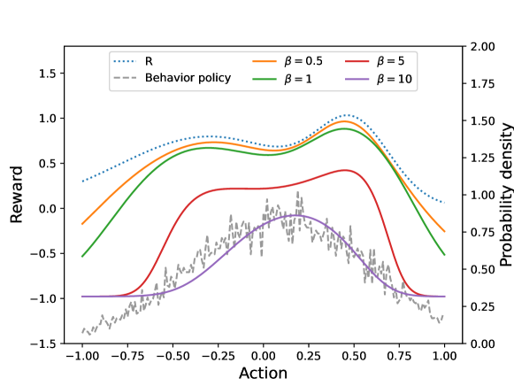
Figure 1: Conservative reward with different $\beta$. $R$ and the behavior policy are also shown for comparison.

Experiments on D4RL

Dataset	Model-based methods						Model-free methods
	CROP	RAMBO	CABI+	MoREL	COMBO	Count-	ATAC	CQL	IQL
	(ours)		TD3-BC			MORL
halfcheetah-random	33.3$\pm$2.8	40.0	15.1	25.6	38.8	41.0	3.9	35.4	-
hopper-random	19.1$\pm$11.0	11.5	11.9	37.3	7.0	30.7	17.5	10.8	-
walker2d-random	21.6$\pm$0.8	21.6	6.4	53.6	17.9	21.9	6.8	7.0	-
halfcheetah-medium	68.1$\pm$0.8	77.6	45.1	42.1	54.2	76.5	53.3	44.4	47.4
hopper-medium	100.6$\pm$3.2	92.8	105.0	95.4	97.2	103.6	85.6	86.6	66.3
walker2d-medium	89.7$\pm$0.8	86.9	82.0	77.8	81.9	87.6	89.6	74.5	78.3
halfcheetah-medium-expert	91.1$\pm$1.1	93.7	107.6	53.3	90.0	100.0	94.8	62.4	86.7
hopper-medium-expert	96.5$\pm$10.2	83.3	112.4	108.7	111.1	111.4	111.9	111.0	91.5
walker2d-medium-expert	109.3$\pm$0.3	68.3	108.6	95.6	103.3	112.3	114.2	98.7	109.6
halfcheetah-medium-replay	64.9$\pm$1.1	68.9	44.4	40.2	55.1	71.5	48.0	46.2	44.2
hopper-medium-replay	93.0$\pm$2.2	96.6	31.3	93.6	89.5	101.7	102.5	48.6	94.7
walker2d-medium-replay	89.7$\pm$0.7	85.0	29.4	49.8	56.0	87.7	92.5	32.6	73.9
mean	73.1	68.9	58.3	64.4	66.8	78.8	68.4	54.9	-

• The highest score on each dataset is underlined. Boldface denotes performance better than 90% of the highest score.

Table 2: Results on the Mujoco tasks of D4RL dataset

In this section, the proposed method CROP is compared with several prior offline RL methods on the Mujoco-v2 tasks (HalfCheetah, Hopper, Walker2D) of D4RL dataset (Fu et al. 2020). Each task has four datasets, Random, Medium, Medium-Replay, and Medium-Expert. The Random dataset comprises transitions gathered through a random policy. The Medium dataset consists of suboptimal data collected by an early-stopped SAC policy. The Medium-Replay dataset encompasses the replay buffer generated during the training of an early-stopped SAC policy. Lastly, the Medium-Expert dataset combines expert demonstrations and suboptimal data.

Due to the different sizes and behavior policies of different datasets, the coverage of offline data and the learned model accuracy are different, which affect the selection of conservatism coefficient $\beta$ and roll-out length $k$. For each dataset, $\beta$ is searched from $\{0.01,0.05,0.1,0.2\}$ and $k$ is searched from $\{3,5,10\}$. We train an ensemble of 7 models and pick the best 5 models based on their loss on the valid set. For the Hopper task, the hidden units of Q-function are 256, while the hidden units of Q-function are 512 for the Halfcheetah task and the Walker2d task. Other hyperparameters are shown in Table. 1.

The performance is compared with several state-of-the-art model-based ( RAMBO (Rigter, Lacerda, and Hawes 2022), CABI+TD3-BC (Lyu, Li, and Lu 2022), MoREL (Kidambi et al. 2020), COMBO (Yu et al. 2021),and Count-MORL (Kim and Oh 2023)) and model-free (ATAC (Cheng et al. 2022), CQL (Kumar et al. 2020), and IQL (Kostrikov, Nair, and Levine 2022)) offline RL methods. Results of the baselines are taken from their respective papers. The score of CROP is the average of the last five evaluations on three random seeds.

The results are shown in the Table. 2. CROP achieves comparable performances (surpassing 90% of the maximum score) on 6 of the 12 datasets and obtains a mean score of 73.1. The proposed method ranks second only to Count-MORL, surpassing the performance of other baselines. This outcome highlights the efficacy of CROP. It should be emphasized that CROP performs better than methods that incorporate conservatism within the value function (COMBO) or the entire environment model (RAMBO), underscoring the value of the novel design choice to introduce conservatism into the reward estimator.

Conclusion

This paper proposes a novel model-based offline RL method CROP which uses a conservative reward estimation. The proposed method estimates the reward by concurrently minimizing both the estimation error and the rewards with random actions during model training. Theoretical analysis shows that CROP can conservatively estimate Q-function, effectively mitigate distribution drift, and ensure a safe policy improvement. Experiments on D4RL benchmarks show that CROP is comparable with the state-of-the-art offline RL methods. CROP provides a new perspective where online RL methods can be used on the empirical MDP with conservative rewards for offline RL problems, which is conducive to applying the latest development of online RL to offline settings. Future work will consider hyperparameter selection without relying on online evaluation. Additionally, combining model design in online model-based RL with CROP will be an appealing way to deal with more complex offline environments.

References

- Agarwal, Jiang, and Kakade (2019) Agarwal, A.; Jiang, N.; and Kakade, S. M. 2019. Reinforcement learning: Theory and algorithms. Seattle, WA: CS Dept. of UW Seattle.
- Agarwal, Schuurmans, and Norouzi (2019) Agarwal, R.; Schuurmans, D.; and Norouzi, M. 2019. An Optimistic Perspective on Offline Reinforcement Learning. In International Conference on Machine Learning.
- An et al. (2021) An, G.; Moon, S.; Kim, J.; and Song, H. O. 2021. Uncertainty-Based Offline Reinforcement Learning with Diversified Q-Ensemble. In Ranzato, M.; Beygelzimer, A.; Dauphin, Y. N.; Liang, P.; and Vaughan, J. W., eds., Annual Conference on Neural Information Processing Systems 2021, 7436–7447.
- Bai et al. (2022) Bai, C.; Wang, L.; Yang, Z.; Deng, Z.; Garg, A.; Liu, P.; and Wang, Z. 2022. Pessimistic Bootstrapping for Uncertainty-Driven Offline Reinforcement Learning. In The Tenth International Conference on Learning Representations.
- Bhardwaj et al. (2023) Bhardwaj, M.; Xie, T.; Boots, B.; Jiang, N.; and Cheng, C.-A. 2023. Adversarial Model for Offline Reinforcement Learning. ArXiv, abs/2302.11048.
- Cheng et al. (2022) Cheng, C.-A.; Xie, T.; Jiang, N.; and Agarwal, A. 2022. Adversarially Trained Actor Critic for Offline Reinforcement Learning. In Proceedings of the 39th International Conference on Machine Learning, 3852–3878.
- Fu et al. (2020) Fu, J.; Kumar, A.; Nachum, O.; Tucker, G.; and Levine, S. 2020. D4RL: Datasets for Deep Data-Driven Reinforcement Learning. ArXiv, abs/2004.07219.
- Fujimoto and Gu (2021) Fujimoto, S.; and Gu, S. S. 2021. A Minimalist Approach to Offline Reinforcement Learning. In Advances in Neural Information Processing Systems 34: Annual Conference on Neural Information Processing Systems 2021, 20132–20145.
- Fujimoto, Meger, and Precup (2019) Fujimoto, S.; Meger, D.; and Precup, D. 2019. Off-Policy Deep Reinforcement Learning without Exploration. In Proceedings of the 36th International Conference on Machine Learning, volume 97, 2052–2062.
- Ghasemipour, Schuurmans, and Gu (2021) Ghasemipour, S. K. S.; Schuurmans, D.; and Gu, S. S. 2021. EMaQ: Expected-Max Q-Learning Operator for Simple Yet Effective Offline and Online RL. In Proceedings of the 38th International Conference on Machine Learning, volume 139, 3682–3691.
- Haarnoja et al. (2018) Haarnoja, T.; Zhou, A.; Hartikainen, K.; Tucker, G.; Ha, S.; Tan, J.; Kumar, V.; Zhu, H.; Gupta, A.; Abbeel, P.; and Levine, S. 2018. Soft Actor-Critic Algorithms and Applications. CoRR, abs/1812.05905.
- Kalashnikov et al. (2018) Kalashnikov, D.; Irpan, A.; Pastor, P.; Ibarz, J.; Herzog, A.; Jang, E.; Quillen, D.; Holly, E.; Kalakrishnan, M.; Vanhoucke, V.; and Levine, S. 2018. QT-Opt: Scalable Deep Reinforcement Learning for Vision-Based Robotic Manipulation. ArXiv, abs/1806.10293.
- Kidambi et al. (2020) Kidambi, R.; Rajeswaran, A.; Netrapalli, P.; and Joachims, T. 2020. MOReL: Model-Based Offline Reinforcement Learning. In Advances in Neural Information Processing Systems 33: Annual Conference on Neural Information Processing Systems 2020, NeurIPS 2020, December 6-12, 2020, virtual.
- Kim and Oh (2023) Kim, B.; and Oh, M. 2023. Model-based Offline Reinforcement Learning with Count-based Conservatism. In the 40 th International Conference on Machine Learning.
- Kostrikov et al. (2021) Kostrikov, I.; Fergus, R.; Tompson, J.; and Nachum, O. 2021. Offline Reinforcement Learning with Fisher Divergence Critic Regularization. In Proceedings of the 38th International Conference on Machine Learning, volume 139 of Proceedings of Machine Learning Research, 5774–5783. PMLR.
- Kostrikov, Nair, and Levine (2022) Kostrikov, I.; Nair, A.; and Levine, S. 2022. Offline Reinforcement Learning with Implicit Q-Learning. In The Tenth International Conference on Learning Representations, ICLR 2022, Virtual Event, April 25-29, 2022.
- Kumar et al. (2019) Kumar, A.; Fu, J.; Soh, M.; Tucker, G.; and Levine, S. 2019. Stabilizing Off-Policy Q-Learning via Bootstrapping Error Reduction. In Advances in Neural Information Processing Systems 32: Annual Conference on Neural Information Processing Systems 2019, NeurIPS 2019, December 8-14, 2019, Vancouver, BC, Canada, 11761–11771.
- Kumar et al. (2020) Kumar, A.; Zhou, A.; Tucker, G.; and Levine, S. 2020. Conservative Q-Learning for Offline Reinforcement Learning. In Proceedings of Annual Conference on Neural Information Processing Systems 2020, 1179–1191.
- Laroche, Trichelair, and des Combes (2019) Laroche, R.; Trichelair, P.; and des Combes, R. T. 2019. Safe Policy Improvement with Baseline Bootstrapping. In Chaudhuri, K.; and Salakhutdinov, R., eds., Proceedings of the 36th International Conference on Machine Learning, ICML 2019, 9-15 June 2019, Long Beach, California, USA, volume 97 of Proceedings of Machine Learning Research, 3652–3661. PMLR.
- Levine et al. (2020) Levine, S.; Kumar, A.; Tucker, G.; and Fu, J. 2020. Offline Reinforcement Learning: Tutorial, Review, and Perspectives on Open Problems. ArXiv, abs/2005.01643.
- Lu et al. (2022) Lu, C.; Ball, P. J.; Parker-Holder, J.; Osborne, M. A.; and Roberts, S. J. 2022. Revisiting Design Choices in Offline Model Based Reinforcement Learning. In The Tenth International Conference on Learning Representations. OpenReview.net.
- Lyu, Li, and Lu (2022) Lyu, J.; Li, X.; and Lu, Z. 2022. Double Check Your State Before Trusting It: Confidence-Aware Bidirectional Offline Model-Based Imagination. In NeurIPS.
- Lyu et al. (2022) Lyu, J.; Ma, X.; Li, X.; and Lu, Z. 2022. Mildly Conservative Q-Learning for Offline Reinforcement Learning. In Annual Conference on Neural Information Processing Systems 2022.
- Mnih et al. (2015) Mnih, V.; Kavukcuoglu, K.; Silver, D.; Rusu, A. A.; Veness, J.; Bellemare, M. G.; Graves, A.; Riedmiller, M. A.; Fidjeland, A. K.; Ostrovski, G.; Petersen, S.; Beattie, C.; Sadik, A.; Antonoglou, I.; King, H.; Kumaran, D.; Wierstra, D.; Legg, S.; and Hassabis, D. 2015. Human-level control through deep reinforcement learning. Nature, 518: 529–533.
- Rafailov et al. (2021) Rafailov, R.; Yu, T.; Rajeswaran, A.; and Finn, C. 2021. Offline Reinforcement Learning from Images with Latent Space Models. In the 3rd Annual Conference on Learning for Dynamics and Control, volume 144, 1154–1168.
- Rigter, Lacerda, and Hawes (2022) Rigter, M.; Lacerda, B.; and Hawes, N. 2022. RAMBO-RL: Robust Adversarial Model-Based Offline Reinforcement Learning. In NeurIPS.
- Shi et al. (2022) Shi, L.; Li, G.; Wei, Y.; Chen, Y.; and Chi, Y. 2022. Pessimistic Q-Learning for Offline Reinforcement Learning: Towards Optimal Sample Complexity. In International Conference on Machine Learning, volume 162, 19967–20025.
- Sun et al. (2023) Sun, Y.; Zhang, J.; Jia, C.; Lin, H.; Ye, J.; and Yu, Y. 2023. Model-Bellman Inconsistency for Model-based Offline Reinforcement Learning. In the 40 th International Conference on Machine Learning.
- Sutton and Barto (2005) Sutton, R. S.; and Barto, A. G. 2005. Reinforcement Learning: An Introduction. IEEE Transactions on Neural Networks, 16: 285–286.
- Yu et al. (2021) Yu, T.; Kumar, A.; Rafailov, R.; Rajeswaran, A.; Levine, S.; and Finn, C. 2021. COMBO: Conservative Offline Model-Based Policy Optimization. In Ranzato, M.; Beygelzimer, A.; Dauphin, Y. N.; Liang, P.; and Vaughan, J. W., eds., Advances in Neural Information Processing Systems 34: Annual Conference on Neural Information Processing Systems 2021, NeurIPS 2021, December 6-14, 2021, virtual, 28954–28967.
- Yu et al. (2020) Yu, T.; Thomas, G.; Yu, L.; Ermon, S.; Zou, J. Y.; Levine, S.; Finn, C.; and Ma, T. 2020. MOPO: Model-based Offline Policy Optimization. In Advances in Neural Information Processing Systems 33: Annual Conference on Neural Information Processing Systems 2020, NeurIPS 2020, December 6-12, 2020, virtual.
- Zhang et al. (2017) Zhang, S.; Yao, L.; Sun, A.; Tay, Y.; Zhang, S.; Yao, L.; and Sun, A. 2017. Deep Learning based Recommender System: A Survey and New Perspectives. ArXiv, abs/1707.07435.