Geometry of exactness of moment-SOS relaxations for polynomial optimization

Abstract

The moment-SOS (sum of squares) hierarchy is a powerful approach for solving globally non-convex polynomial optimization problems (POPs) at the price of solving a family of convex semidefinite optimization problems (called moment-SOS relaxations) of increasing size, controlled by an integer, the relaxation order. We say that a relaxation of a given order is exact if solving the relaxation actually solves the POP globally. In this note, we study the geometry of the exactness cone, defined as the set of polynomial objective functions for which the relaxation is exact. Generalizing previous foundational work on quadratic optimization on real varieties, we prove by elementary arguments that the exactness cones are unions of semidefinite representable cones monotonically embedded for increasing relaxation order.

1 Solving POPs with the moment-SOS hierarchy

Given a compact semialgebraic set ${\mathscr{X}}\in\mathbb{R}^{n}$ and a polynomial $f$ in the vector space $\mathbb{R}[{\bf x}]_{d}$ of polynomials of ${\bf x}\in\mathbb{R}^{n}$ of degree up to $d$, consider the polynomial optimization problem (POP)

$$v(f):=\min_{{\bf x}\in{\mathscr{X}}}f({\bf x}).$$ (1)

The notation emphasizes that the optimal value depends parametrically on the objective function.

The key observation behind the moment-SOS (sum of squares) hierarchy [7, 5, 4, 8] is that the POP is equivalent to the primal-dual problems

$$\begin{array}[]{rcllcll}v(f)&=&\min_{{\bf y}}&\ell_{{\bf y}}(f)&=&\max_{v}&v\\ &&\mathrm{s.t.}&{\bf y}\in{\mathscr{M}}({\mathscr{X}})_{d}&&\mathrm{s.t.}&f-v\in{\mathscr{P}}({\mathscr{X}})_{d}\\ &&&\ell_{{\bf y}}(1)=1\end{array}$$

where the dual maximization problem consists of finding the largest lower bound $v\in\mathbb{R}$ on $f$ on ${\mathscr{X}}$, formalized as a linear conic problem in the convex cone ${\mathscr{P}}({\mathscr{X}})_{d}$ of polynomials of degree up to $d$ which are positive on ${\mathscr{X}}$. The primal minimization problem is over vectors ${\bf y}$ in the convex cone ${\mathscr{M}}({\mathscr{X}})_{d}$ of moments of degree up to $d$ of positive measures on ${\mathscr{X}}$, which is the convex dual of ${\mathscr{P}}({\mathscr{X}})_{d}$, defined as the set of linear functionals positive on ${\mathscr{P}}({\mathscr{X}})_{d}$, cf. e.g. [8, Thm. 8.1.2]. The linear objective function in the primal conic problem is $\ell_{{\bf y}}(f):=\int_{{\mathscr{X}}}f({\bf x})d\mu({\bf x})$ where $\mu$ is a positive measure with moment vector ${\bf y}$, and the linear constraint $\ell_{{\bf y}}(1)=\int_{{\mathscr{X}}}d\mu({\bf x})=1$ enforces that $\mu$ is a probability measure.

If ${\mathscr{X}}:=\{{\bf x}\in\mathbb{R}^{n}:g_{i}({\bf x})\geq 0,i=1,\ldots,m\}$ is basic semialgebraic, defined by a given polynomial vector ${\bf g}=(g_{i})_{i=1,\ldots,m}$, then ${\mathscr{P}}({\mathscr{X}})_{d}$ can be approximated with other convex cones, the truncated quadratic modules

$${\mathscr{Q}}({\bf g})^{r}_{d}:=\{p\in\mathbb{R}[{\bf x}]_{d}:p=\sum_{i=0}^{m}s_{i}g_{i},\>s_{i}\in\Sigma[{\bf x}],\>s_{i}g_{i}\in\mathbb{R}[{\bf x}]_{2r}\}$$

where $\Sigma[{\bf x}]\subset\mathbb{R}[{\bf x}]$ is the convex cone of sums of squares (SOS) of polynomials of ${\bf x}$ and $g_{0}({\bf x}):=1$.

Remark 1.

Note that if a polynomial equation enters the definition of ${\mathscr{X}}$, i.e. $g_{i}({\bf x})=0$ instead of $g_{i}({\bf x})\geq 0$ for some $i=1,\ldots,m$, then the corresponding weight $s_{i}\in\mathbb{R}[{\bf x}]$ in the quadratic module ${\mathscr{Q}}({\bf g})^{r}_{d}$ is not constrained in sign, while satisfying $s_{i}g_{i}\in\mathbb{R}[{\bf x}]_{2r}$. This is consistent with the fact that two inequalities of opposite signs are equivalent to an equation. Without loss of generality, and for notational conciseness, in this note we use only inequalities.

Note that by construction the quadratic modules are monotonically embedded for decreasing relaxation order:

$${\mathscr{Q}}({\bf g})^{r}_{d}\subset{\mathscr{Q}}({\bf g})^{r+1}_{d}\subset{\mathscr{P}}({\mathscr{X}})_{d}.$$ (2)

Contrary to ${\mathscr{P}}({\mathscr{X}})_{d}$, the truncated quadratic module ${\mathscr{Q}}({\bf g})^{r}_{d}$ is semidefinite representable, i.e. it is the linear projection of a spectrahedron, itself defined as a linear section of the cone of positive semidefinite quadratic forms. Practically, this means that linear optimization in ${\mathscr{Q}}({\bf g})^{r}_{d}$ can be done efficiently with powerful interior-point algorithms.

Let us denote by ${\mathscr{R}}({\bf g})^{r}_{d}$ the convex cone dual to the truncated quadratic module ${\mathscr{Q}}({\bf g})^{r}_{d}$. By convex duality, for the primal problem we have the reversed monotone embedding ${\mathscr{R}}({\bf g})^{r}_{d}\supset{\mathscr{R}}({\bf g})^{r+1}_{d}\supset{\mathscr{M}}({\bf g})_{d}$ meaning that the moment cone is approximated from outside, or relaxed. This motivates the terminology moment relaxation to refer to ${\mathscr{R}}({\bf g})^{r}_{d}$.

Now we have all the ingredients to define the moment-SOS hierarchy also known as Lasserre’s hierarchy: a family of primal-dual convex semidefinite optimization problems whose size is controlled by the relaxation order $r\in\mathbb{N}$:

$$\begin{array}[]{rcllcll}v^{r}(f)&:=&\inf_{{\bf y}}&\ell_{{\bf y}}(f)&\geq&\sup_{v}&v\\ &&\mathrm{s.t.}&{\bf y}\in{\mathscr{R}}({\bf g})^{r}_{d}&&\mathrm{s.t.}&f-v\in{\mathscr{Q}}({\bf g})^{r}_{d}\\ &&&\ell_{{\bf y}}(1)=1.\end{array}$$ (3)

This primal-dual pair of semidefinite optimization problems is called the moment-SOS relaxation of order $r$

Assumption 1.

For large enough $R\in\mathbb{R}$ and $r\in\mathbb{N}$ it holds $R^{2}-\sum_{k=1}^{n}x^{2}_{i}\in{\mathscr{Q}}({\bf g})^{r}_{2}$.

Since ${\mathscr{X}}$ is bounded, it is always possible to add a redundant quadratic constraint $R^{2}-\sum_{k=1}^{n}x^{2}_{i}\geq 0$ to the description of ${\mathscr{X}}$. So Assumption 1 is without loss of generality. Then it follows from [6] that the relaxed values are monotonically converging lower bounds on the value:

$$v^{r}(f)\leq v^{r+1}(f)\leq v^{\infty}(f)=v(f),$$ (4)

that the primal is attained (i.e. the infimum is a minimum) and that there is no duality gap (i.e. the infimum equals the supremum). Moreover if ${\mathscr{X}}$ has an interior point, then the dual is attained (i.e. the supremum is a maximum). If ${\mathscr{X}}$ does not have an interior point, e.g. if it is a low-dimensional algebraic variety, then additional algebraic or geometric conditions are required for the dual to be attained, cf. [2, 1, 8].

2 Exactness cone

Beyond the asymptotic convergence guarantees (4), it is important to know whether the moment-SOS relaxation of a given order is exact, i.e. whether an optimal solution to the relaxation attains the value $v(f)$. If this is the case, there is no need to increase $r$ and solve larger semidefinite optimization problems.

In this note, we are interested in the geometry of the exactness cone, defined as the set of objective functions which are such that the moment-SOS relaxation (3) is exact.

Definition 1.

The exactness cone of degree $d$ at relaxation order $r$ is defined by

$${\mathscr{F}}({\bf g})^{r}_{d}:=\{f\in\mathbb{R}[{\bf x}]_{d}:\ell_{\hat{{\bf y}}}(f)=\hat{v}=v(f),\>\hat{{\bf y}}\in{\mathscr{R}}({\bf g})^{r}_{d},\>f-\hat{v}\in{\mathscr{Q}}({\bf g})^{r}_{d}\}.$$

Note that this set is a cone since $v(af)=av(f)$ for all $a\geq 0$.

Our main result states that the exactness cone is a (generally uncountable and non-convex) union of semidefinite representable cones. We also describe the convex geometry of the exactness cones, their monotone embedding, and how they are related to normal cones of the moment relaxations.

Our analysis is elementary. It is inspired by the foundational work [3] which focused on the particular case of the Shor relaxation ($r=1$) with $f$ linear ($d=1$) or quadratic ($d=2$), and ${\mathscr{X}}$ a real algebraic variety defined by quadratic equations. We believe that our contribution consists of considerably simplifying and extending this analysis to higher order relaxations of general semialgebraic sets.

3 Main result

Theorem 1.

The exactness cone at relaxation order $r$ is given by

$${\mathscr{F}}({\bf g})^{r}_{d}=\bigcup_{\hat{{\bf x}}\in{\mathscr{X}}}{\mathscr{S}}_{\hat{{\bf x}}}({\bf g})^{r}_{d}$$ (5)

where each cone

$${\mathscr{S}}_{\hat{{\bf x}}}({\bf g})^{r}_{d}:=\{f\in{\mathscr{Q}}({\bf g})^{r}_{d},\>f(\hat{{\bf x}})=0\}$$

is semidefinite representable.

Proof: At order $r$, exactness of the moment-SOS relaxation (3) is equivalent to the existence of an optimal primal-dual pair ($\hat{{\bf y}},\hat{v}$) with a Dirac vector $\hat{{\bf y}}\in{\mathscr{R}}({\bf g})^{r}_{d}$ concentrated at a point $\hat{{\bf x}}\in{\mathscr{X}}$, i.e. such that the objective function is the point evaluation $v^{r}(f)=\ell_{\hat{{\bf y}}}(f)=f(\hat{{\bf x}})=\hat{v}$, and also $f-\hat{v}\in{\mathscr{Q}}({\bf g})^{r}_{d}$. Since $\hat{{\bf x}}\in{\mathscr{X}}$, the value $f(\hat{{\bf x}})$ is an upper bound on the global optimum $v(f)$. According to (4), $v^{r}(f)$ is also a lower bound, so it follows that $v^{r}(f)=v(f)$.

Optimality of a primal-dual pair $(\hat{{\bf y}},\hat{v})$ is equivalent to conic complementarity of $\hat{{\bf y}}\in{\mathscr{R}}({\bf g})^{r}_{d}$ and $f-\hat{v}\in{\mathscr{Q}}({\bf g})^{r}_{d}$, i.e. $\ell_{\hat{{\bf y}}}(f)-\hat{v}=f(\hat{{\bf x}})-\hat{v}=f(\hat{{\bf x}})-v(f)=0$. Therefore, for each $\hat{{\bf x}}\in{\mathscr{X}}$, objective functions $f\in\mathbb{R}[{\bf x}]_{d}$ that achieve exactness are such that $f=v(f)+f^{0}$ for some polynomial $f^{0}\in{\mathscr{Q}}({\bf g})^{r}_{d}$. This polynomial satisfies $f^{0}(\hat{{\bf x}})=f(\hat{{\bf x}})-v(f)=0$, i.e. it belongs to ${\mathscr{S}}_{\hat{{\bf x}}}({\bf g})^{r}_{d}$.

Cone ${\mathscr{S}}_{\hat{{\bf x}}}({\bf g})^{r}_{d}$ is semidefinite representable since it is the projection of linear sections of the SOS cone $\Sigma[{\bf x}]$, which is itself semidefinite representable.

The proof is completed by observing that ${\mathscr{S}}_{\hat{{\bf x}}}({\bf g})^{r}_{d}$ reduces to the origin whenever $\hat{{\bf x}}$ is not optimal for POP (1). Let us proceed by contradiction. Let $\hat{{\bf x}}\in{\mathscr{X}}$ be non-optimal, and assume there exists a non-zero polynomial $f^{0}\in{\mathscr{S}}_{\hat{{\bf x}}`}({\bf g})^{r}_{d}$, i.e. $f^{0}(\hat{{\bf x}})=0$. Since $\hat{{\bf x}}$ is not optimal, $f^{0}(\hat{{\bf x}})=f(\hat{{\bf x}})-v(f)>0$, a contradiction. $\Box$

Remark 2.

The truncated quadratic module ${\mathscr{Q}}({\bf g})^{r}_{d}$ can be replaced by any other semidefinite representable approximation of ${\mathscr{P}}({\mathscr{X}})$, e.g. the preordering of ${\bf g}$, or any other Positivstellensatz [7, 8].

Remark 3.

The exactness cone is semialgebraic since $f$ belongs to ${\mathscr{F}}({\bf g})^{r}_{d}$ whenever 1) $f$ belongs to ${\mathscr{Q}}({\bf g})^{r}_{d}$, a semidefinite representable hence semialgebraic cone, and 2) there exists $\hat{{\bf x}}$ in ${\mathscr{X}}$, a semialgebraic set, such that $f$ vanishes at $\hat{{\bf x}}$.

Remark 4.

It follows from the proof of Theorem 1 that it is enough to restrict the union (5) to points $\hat{{\bf x}}\in{\mathscr{X}}$ which are optimal for some objective function $f$. For example if $d=1$, the union can be restricted to the set of extreme points of the convex hull of ${\mathscr{X}}$. In general however it is not easy to describe explicitly these subsets of ${\mathscr{X}}$.

Remark 5.

In our definition of the exactness cone, we require that both primal and dual values are attained in (3). Since what matters is whether $v^{r}(f)=v(f)$, we may relax our attainment requirements. The corresponding exactness cones would be slightly larger, at the price of more technicalities.

4 Geometry of exactness cones

Lemma 1.

The exactness cones are monotonically embedded for increasing relaxation order:

$$\mathbb{R}[{\bf x}]_{0}\subset{\mathscr{F}}({\bf g})^{r}_{d}\subset{\mathscr{F}}({\bf g})^{r+1}_{d}\subset\overline{{\mathscr{F}}({\bf g})^{\infty}_{d}}=\mathbb{R}[{\bf x}]_{d}.$$

Proof: The inclusion $R[{\bf x}]_{0}\subset{\mathscr{F}}({\bf g})^{r}_{d}$ follows from the translation invariance of the value: $v(f+a)=v(f)+a$ for all $a\in\mathbb{R}$. The inclusion ${\mathscr{F}}({\bf g})^{r}_{d}\subset{\mathscr{F}}({\bf g})^{r+1}_{d}$ follows from the inclusion relations (2). Finally, the identity $\overline{{\mathscr{F}}({\bf g})^{\infty}_{d}}=\mathbb{R}[{\bf x}]_{d}$ follows from Putinar’s Positivstellensatz – see e.g. [7, Thm. 2.15] – which states that under Assumption 1 every strictly positive polynomial of degree $d$ on ${\mathscr{X}}$ belongs to ${\mathscr{Q}}({\bf g})^{r}_{d}$ for sufficiently large $r\in\mathbb{N}$, i.e. $\overline{{\mathscr{Q}}({\bf g})^{\infty}_{d}}={\mathscr{P}}({\mathscr{X}})_{d}$. $\Box$

Remark 6.

Note that in Lemma 1 the closure is required for asymptotic exactness of all degree $d$ polynomial objective functions, i.e. $\overline{{\mathscr{F}}({\bf g})^{\infty}_{d}}=\mathbb{R}[{\bf x}]_{d}$. A classical example is $n=m=1$, $g_{1}(x)=-x^{2}$ for which ${\mathscr{X}}=\{0\}$ and Assumption 1 is readily satisfied. Whereras $f(x)=\pm x\notin{\mathscr{Q}}({\bf g})^{r}_{1}$ for finite $r\in\mathbb{N}$, it holds that $f(x)+\varepsilon=\frac{\varepsilon}{2}+\frac{\varepsilon}{2}(1\pm\frac{x}{\varepsilon})^{2}-\frac{x^{2}}{2\varepsilon}+\in{\mathscr{Q}}({\bf g})^{1}_{1}$ for every $\varepsilon>0$, see [1, Ex. 1.3.4] or [8, §2.5.2]. For this example ${\mathscr{F}}({\bf g})^{r}_{1}=\mathbb{R}[{\bf x}]_{0}$ for all finite $r$, and $\overline{{\mathscr{F}}({\bf g})^{\infty}_{1}}=\mathbb{R}[{\bf x}]_{1}$.

Given $\hat{{\bf x}}\in{\mathscr{X}}$, let ${\bf y}_{\hat{{\bf x}}}$ be the Dirac vector at $\hat{{\bf x}}$, i.e. such that $\ell_{{\bf y}_{\hat{{\bf x}}}}(f)=f(\hat{{\bf x}})$ for every $f\in\mathbb{R}[{\bf x}]_{d}$. Given a convex set ${\mathscr{Y}}\in\mathbb{R}^{N}$, let ${\mathscr{N}}_{{\mathscr{Y}}}({{\bf y}})$ denote the normal cone to ${\mathscr{Y}}$ at a point ${{\bf y}}\in{\mathscr{Y}}$. Recall that $f\in{\mathscr{N}}_{{\mathscr{Y}}}({{\bf y}})$ if and only if ${{\bf y}}\in\mathrm{argmax}_{{\bf y}\in{\mathscr{Y}}}\ell_{{\bf y}}(f)$, where $\ell_{{\bf y}}(f)$ is a linear functional on $\mathbb{R}^{N}$. With these notations, we have the following geometric counterpart to Theorem 1.

Lemma 2.

Up to the sign, the spectrahedral cones of Theorem 1 are normal cones to the moment relaxation:

$${\mathscr{S}}_{\hat{{\bf x}}}({\bf g})^{r}_{d}=-{\mathscr{N}}_{{\mathscr{R}}({\bf g})^{r}_{d}}({\bf y}_{\hat{{\bf x}}})$$

for all $\hat{{\bf x}}\in{\mathscr{X}}$.

Proof: First observe that extreme points of the moment cone ${\mathscr{M}}({\mathscr{X}})_{d}$ are Dirac vectors of ${\mathscr{X}}$, cf. e.g. [8, Thm. 8.1.1]. Dirac vectors which are also extreme points of the moment relaxation ${{\mathscr{R}}({\bf g})^{r}_{d}}$ are of the form ${{\bf y}}_{\hat{{\bf x}}}$ for some optimal $\hat{{\bf x}}\in{\mathscr{X}}$ for POP (1).

Therefore, if $\hat{{\bf x}}$ is optimal then ${\bf y}_{\hat{{\bf x}}}\in\mathrm{argmin}_{{\bf y}\in{\mathscr{R}}({\bf g})^{r}_{d}}\ell_{{\bf y}_{\hat{{\bf x}}}}(f^{0})$ with $f^{0}:=f-v(f)\in-{\mathscr{N}}_{{\mathscr{R}}({\bf g})^{r}_{d}}({\bf y}_{\hat{{\bf x}}})$, $\ell_{{\bf y}_{\hat{{\bf x}}}}(f^{0})=f^{0}(\hat{{\bf x}})=0$. Since ${\mathscr{Q}}({\bf g})^{r}_{d}$ is dual to ${\mathscr{R}}({\bf g})^{r}_{d}$, it follows that $f^{0}\in{\mathscr{Q}}({\bf g})^{r}_{d}$ and hence $f^{0}\in{\mathscr{S}}_{\hat{{\bf x}}}({\bf g})^{r}_{d}$.

If $\hat{{\bf x}}\in{\mathscr{X}}$ is not optimal, then the Dirac vector ${\bf y}_{\hat{{\bf x}}}$ cannot be on the boundary of the moment relaxation ${{\mathscr{R}}({\bf g})^{r}_{d}}$, so the normal cone ${\mathscr{N}}_{{\mathscr{R}}({\bf g})^{r}_{d}}({\bf y}_{\hat{{\bf x}}})$ at this point is zero, which trivially belongs to ${\mathscr{S}}_{\hat{{\bf x}}}({\bf g})^{r}_{d}$. $\Box$

Lemma 2 is a generalization of [3, Prop. 4.7] which considers only the case $d\leq 2$ and the Shor relaxation (i.e. $r=1$) for real varieties ${\mathscr{X}}$ generated by quadratic polynomials.

It is of interest to know whether we have exactness at relaxation order $r$ for all objective functions. Obviously, a necessary and sufficient condition is that ${\mathscr{R}}({\bf g})^{r}_{d}={\mathscr{M}}({\mathscr{X}})_{d}$, i.e. all vectors of the moment relaxation are convex combinations of Dirac vectors of ${\mathscr{X}}$. If $d=1$ the condition becomes ${\mathscr{R}}({\bf g})^{r}_{1}=\mathbb{R}_{+}\times\mathrm{conv}\>{\mathscr{X}}$, the Cartesian product of the positive real line with the convex hull of ${\mathscr{X}}$.

5 Examples

5.1 Finite set

Let us revisit [3, Ex. 4.4] where $d=1$ and

$$\begin{array}[]{rcl}{\mathscr{X}}&=&\{{\bf x}\in\mathbb{R}^{2}:g_{1}({\bf x})=2x_{2}-2x^{2}_{2}+x_{1}x_{2}=0,\>g_{2}({\bf x})=-x_{1}+x_{2}+x^{2}_{1}-x^{2}_{2}=0\}\\ &=&\{(0,0),(0,1),(1,0),(2,2)\}\end{array}$$

is a finite set consisting of four points. Then the exactness cone ${\mathscr{F}}({\bf g})^{r}_{d}$ is the union of four semidefinite representable cones. For example if $d=r=1$ one of these cones is

$$\begin{array}[]{rcl}{\mathscr{S}}(2,2)^{1}_{1}&=&\{f\in\mathbb{R}[{\bf x}]_{1}:f({\bf x})=f_{0}+f_{1}x_{1}+f_{2}x_{2}=s_{0}({\bf x})+s_{1}g_{1}({\bf x})+s_{2}g_{2}({\bf x}),\\ &&\quad f(2,2)=0,s_{0}\in\Sigma[{\bf x}]\cap\mathbb{R}[{\bf x}]_{2},s_{1}\in\mathbb{R},s_{2}\in\mathbb{R}\}\end{array}$$

which can be written more explicitly by expressing the quadratic SOS constraint

$$s_{0}({\bf x})=(1,x_{1},x_{2})X(1,x_{1},x_{2})^{T},\>X=\left(x_{ij}\right)_{i,j=1,2,3}\succeq 0$$

with a 3-by-3 positive semidefinite Gram matrix $X$, as well as the equality constraint

$$f(2,2)=s_{0}(2,2)=x_{11}+4x_{21}+4x_{22}+4x_{31}+8x_{32}+4x_{33}=0.$$

Therefore

$$\begin{array}[]{rcl}{\mathscr{S}}(2,2)^{1}_{1}&=&\{(f_{0},f_{1},f_{2})\in\mathbb{R}^{3}:f_{0}=x_{11},f_{1}=2x_{21}-s_{2},f_{2}=2x_{31}+2s_{1}+s_{2},\\ &&\quad 0=x_{22}+s_{2},0=2x_{32}+s_{1},0=x_{33}-2s_{1}-s_{2},\\ &&\quad x_{11}+4x_{21}+4x_{22}+4x_{31}+8x_{32}+4x_{33}=0,\\ &&\quad X\succeq 0,s_{1}\in\mathbb{R},s_{2}\in\mathbb{R}\}\\ &&=\{(f_{0},f_{1},f_{2})\in\mathbb{R}^{3}:\left(\begin{array}[]{ccc}2f_{0}&f_{1}+s_{2}&f_{2}-2s_{1}+s_{2}\\ f_{1}+s_{2}&-2s_{2}&-s_{1}\\ f_{2}-2s_{1}+s_{2}&-s_{1}&4s_{1}+2s_{2}\end{array}\right)\succeq 0,s_{1}\in\mathbb{R},s_{2}\in\mathbb{R}\}\end{array}$$

is the 3-dimensional projection of a 5-dimensional cubic spectrahedral cone.

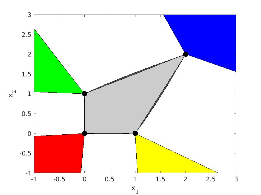
(a) First moment relaxation and normal cones

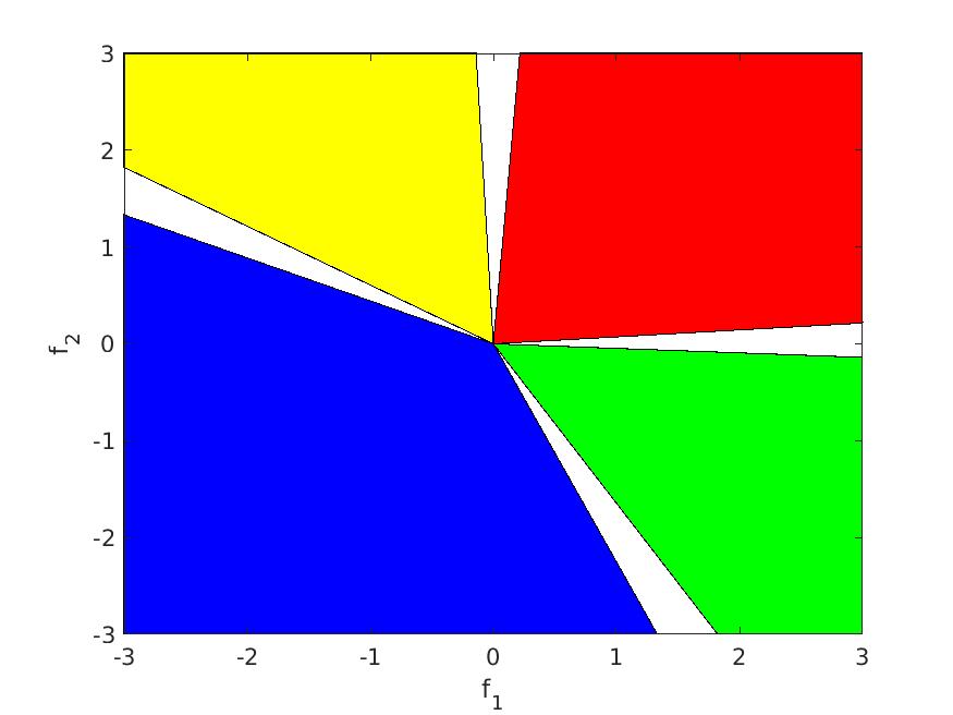
(b) First exactness cone

Figure 1: Finite set. Left (a): first moment relaxation (dark gray) including the convex hull (light gray) of ${\mathscr{X}}$ (four black points), and normal cones at the points (colored). Right (b): first exactness cone (colored).

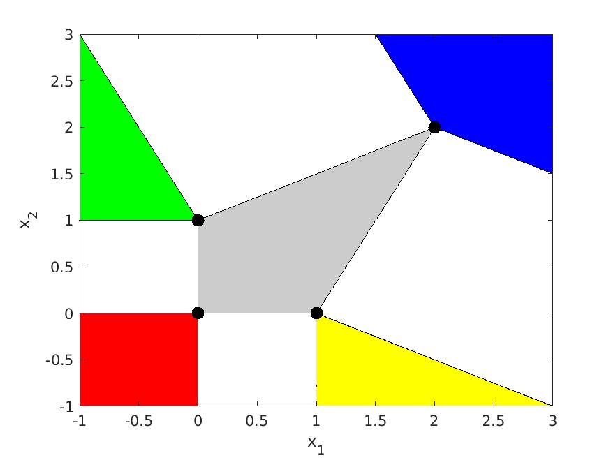
(a) Second moment relaxation and normal cones

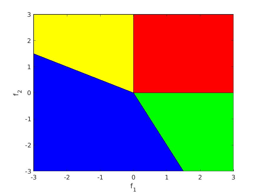
(b) Second exactness cone

Figure 2: Finite set. Left (a): second moment relaxation (light gray) which is the convex hull of ${\mathscr{X}}$ (four black points), and normal cones at the points (colored). Right (b): second exactness cone (colored).

On the left of Figure 1 we represent the first ($r=1$) moment relaxation ${\mathscr{R}}({\bf g})^{1}_{1}$ (dark gray), the convex hull $\mathrm{conv}\>{\mathscr{X}}$ (light gray), and the four points of ${\mathscr{X}}$ (black). The tiny dark gray region which remains visible are points in ${\mathscr{R}}({\bf g})^{1}_{1}\setminus\mathrm{conv}\>{\mathscr{X}}$. Also represented (in color) are the four normal cones at the four points. According to Lemma 2, up to the sign, they are the four spectrahedral cones ${\mathscr{S}}(\hat{{\bf x}})$, $\hat{{\bf x}}\in{\mathscr{X}}$ of Theorem 1. On the right of Figure 1 we represent the exactness cone ${\mathscr{F}}({\bf g})^{1}_{1}$ which is the union of the four spectrahedra, according to Theorem 1. We observe tiny conic regions (in white) corresponding to $\mathbb{R}[{\bf x}]_{1}\setminus{\mathscr{F}}({\bf g})^{1}_{1}$, namely first degree polynomials $f$ for which the moment-SOS relaxation of first order is not exact. If we solve the relaxation, we hit the slightly inflated tiny regions (dark gray on the left figure) of the moment relaxation ${\mathscr{R}}({\bf g})^{1}_{1}$, yielding a strict lower bound on the value $v(f)$. If instead we minimize the polynomials in ${\mathscr{F}}({\bf g})^{1}_{1}$, we hit one of the four points of ${\mathscr{X}}$, i.e. the relaxation is exact.

On Figure 2 we represent the same objects for the second relaxation, i.e. $r=2$. On the left, we see that the moment relaxation ${\mathscr{R}}({\bf g})^{2}_{1}$ is the polytope $\mathrm{conv}\>{\mathscr{X}}$, i.e. ${\mathscr{R}}({\bf g})^{2}_{1}\setminus\mathrm{conv}\>{\mathscr{X}}$ is empty: the tiny dark gray regions of Figure 1(a) disappeared. Consistently with Lemma LABEL:polytope, we observe on the right that the exactness cone ${\mathscr{F}}({\bf g})^{2}_{1}$ is the whole space $\mathbb{R}[{\bf x}]_{1}$, i.e. the relaxation is exact everywhere: the tiny white regions of Figure 1(b) disappeared, consistently with Lemma 1. Exactness follows from the property that all non-negative bivariate quartics are SOS. Indeed, the dual problem consists of maximizing $v$ such that $f-v$ is positive on the four points of ${\mathscr{X}}$, a linear constraint. But this is equivalent to enforcing that $f-v$ is a degree 4 (i.e. $r=2$) SOS subject to the linear constraint.

5.2 Non-convex set

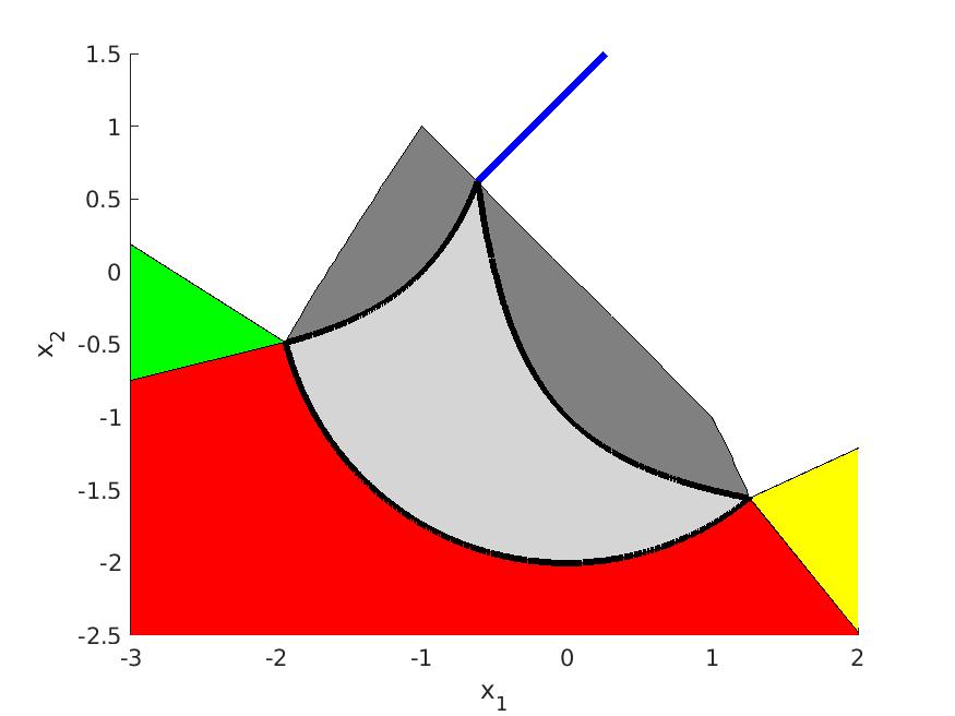
(a) First moment relaxation and normal cones

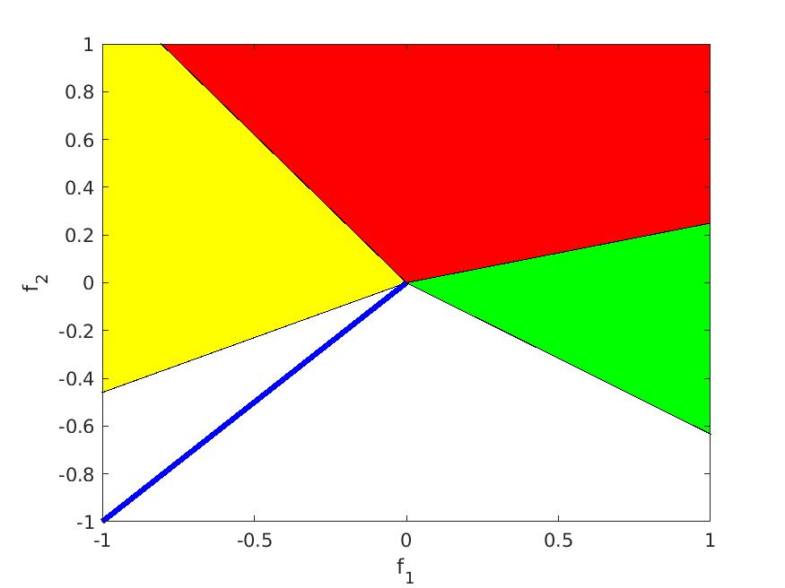
(b) First exactness cone

Figure 3: Non-convex set. Left (a): first moment relaxation (dark gray) of ${\mathscr{X}}$ (light gray), and normal cones (colored). Right (b): first exactness cone (colored).

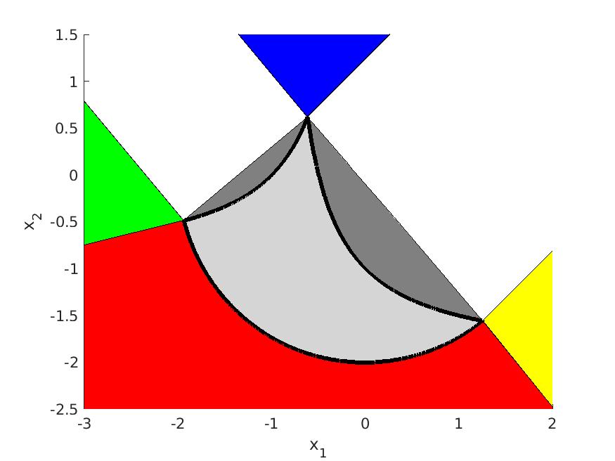
(a) Second moment relaxation and normal cones

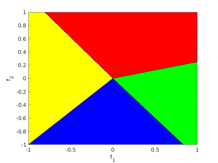
(b) Second exactness cone

Figure 4: Non-convex set. Left (a): second moment relaxation (dark gray) which is the convex hull of ${\mathscr{X}}$ (light gray), and normal cones at the points (colored). Right (b): second exactness cone (colored).

Consider [4, Ex.2 21] where $d=1$ and

$$\begin{array}[]{rcl}{\mathscr{X}}&=&\{{\bf x}\in\mathbb{R}^{2}:g_{1}({\bf x})=4-x^{2}_{1}-x^{2}_{2}\geq 0,\>g_{2}({\bf x})=-1-2x_{1}-x_{2}-x_{1}x_{2}\geq 0,\\ &&\quad g_{3}({\bf x})=1+x_{1}+x_{1}x_{2}\geq 0\}.\end{array}$$

On the left of Figure 3 we represent the first ($r=1$) moment relaxation ${\mathscr{R}}({\bf g})^{1}_{1}$ (dark gray) of ${\mathscr{X}}$ (light gray), as well as the normal cones to the points of the boundary of ${\mathscr{R}}({\bf g})^{1}_{1}$ where the first relaxation is exact. The green region is the normal cone to the left corner point of ${\mathscr{X}}$, the yellow region is the normal cone to the right corner point of ${\mathscr{X}}$, the blue line is the one-dimensional normal cone to the top corner point of ${\mathscr{X}}$, and the red region is the union of all the one-dimensional normal cones to the convex circular bottom part of ${\mathscr{X}}$. According to Lemma 2, up to the sign, the green, yellow, and blue cones are spectrahedral cones, whereas the red region is the union of spectrahedral cones along the circular arc. On the right of Figure 3 we represent the exactness cone ${\mathscr{F}}({\bf g})^{1}_{1}$ which is the union of these spectrahedral cones, according to Theorem 1. The blue line corresponds to the objective function $f({\bf x})=-x_{1}-x_{2}$ for which the first moment relaxation is exact. It is surrounded by a white region corresponding to objective functions for which the first moment relaxation is not exact. The other colored regions belong to the exactness cone.

On the left of Figure 4 we represent the second ($r=2$) moment relaxation ${\mathscr{R}}({\bf g})^{2}_{1}$ (dark gray) of ${\mathscr{X}}$ (light gray), as well as the normal cones to the points of the boundary of ${\mathscr{R}}({\bf g})^{2}_{1}$ where the second relaxation is exact. Observe that ${\mathscr{R}}({\bf g})^{2}_{1}=\mathrm{conv}\>{\mathscr{X}}$. In comparison with Figure 3, we notice that the green and yellow normal cones are now larger, and the blue half-line of the first relaxation is now a full-dimensional normal cone to the top corner of ${\mathscr{X}}$. On the right of Figure 4, we consistently see that the exactness cone ${\mathscr{F}}({\bf g})^{2}_{1}$ now fills up to whole space $\mathbb{R}[{\bf x}]_{1}$, i.e. the second moment relaxation is exact for all first degree objective functions.

References

• [1] L. Baldi. Représentations effectives en géométrie algébrique réelle et optimisation polynomiale. PhD thesis, Inria Univ. Côte d’Azur, 2022.
• [2] L. Baldi, B. Mourrain. Exact moment representation in polynomial optimization arXiv:2012.14652, 2020.
• [3] D. Cifuentes, C. Harris, B. Sturmfels. The geometry of SDP-exactness in quadratic optimization Math. Prog. 182:399-428, 2020.
• [4] D. Henrion. Moments for polynomial optimization - An illustrated tutorial. Lecture notes of a course given for the programme Recent Trends in Computer Algebra, Institut Henri Poincaré, Paris, 2023.
• [5] D. Henrion, M. Korda and J. B. Lasserre. The moment-SOS hierarchy. World Scientific, 2020.
• [6] C. Josz, D. Henrion. Strong duality in Lasserre’s hierarchy for polynomial optimization. Optim. Letters 1(10):3-10, 2016.
• [7] J. B. Lasserre. An introduction to polynomial and semi-algebraic optimization. Cambridge Univ. Press, 2015.
• [8] J. Nie. Moments and polynomial optimization. SIAM, 2023.