LLM4DyG: Can Large Language Models Solve Problems on Dynamic Graphs?

Abstract

In an era marked by the increasing adoption of Large Language Models (LLMs) for various tasks, there is a growing focus on exploring LLMs’ capabilities in handling web data, particularly graph data. Dynamic graphs, which capture temporal network evolution patterns, are ubiquitous in real-world web data. Evaluating LLMs’ competence in understanding spatial-temporal information on dynamic graphs is essential for their adoption in web applications, which remains unexplored in the literature. In this paper, we bridge the gap via proposing to evaluate LLMs’ spatial-temporal understanding abilities on dynamic graphs, to the best of our knowledge, for the first time. Specifically, we propose the LLM4DyG benchmark, which includes nine specially designed tasks considering the capability evaluation of LLMs from both temporal and spatial dimensions. Then, we conduct extensive experiments to analyze the impacts of different data generators, data statistics, prompting techniques, and LLMs on the model performance. Finally, we propose Disentangled Spatial-Temporal Thoughts (DST2) for LLMs on dynamic graphs to enhance LLMs’ spatial-temporal understanding abilities. Our main observations are: 1) LLMs have preliminary spatial-temporal understanding abilities on dynamic graphs, 2) Dynamic graph tasks show increasing difficulties for LLMs as the graph size and density increase, while not sensitive to the time span and data generation mechanism, 3) the proposed DST2 prompting method can help to improve LLMs’ spatial-temporal understanding abilities on dynamic graphs for most tasks. The data and codes will be open-sourced at publication time.

1 Introduction

In an era marked by the increasing adoption of Large Language Models (LLMs) for various tasks beyond natural language processing, such as image recognition (Alayrac et al., 2022), healthcare diagnostics (Thirunavukarasu et al., 2023), and autonomous agents (Wang et al., 2023b), there has been a growing body of research dedicated to exploring LLMs’ abilities to tackle the vast troves of web data. One area of particular interest is the handling of graph data, which ubiquitously exists on the Internet. The World Wide Web itself can be seen as a colossal interconnected graph of webpages, hyperlinks, and content. For example, social media platforms like Facebook and Twitter generate dynamic social graphs reflecting user interactions and connections.

To leverage the in-context learning and commonsense knowledge of LLMs, several pioneer works have been dedicated to adopting LLMs on static graphs. For instance,  Wang et al. (2023a) and  Guo et al. (2023) propose benchmarks to evaluate LLMs’ proficiency in comprehending and reasoning about graph structures, with tasks like graph connectivity, topological sort, etc, demonstrating the LLMs’ abilities of in-context learning and reasoning to solve static graph problems.  Ye et al. (2023) and  Chen et al. (2023b) propose to fine-tune the LLMs to solve graph tasks in natural language, showing the strong potential of LLMs to leverage text information, generate human-readable explanations, and integrate commonsense knowledge to enhance the reasoning over structures.

Dynamic graphs, in comparison with static graphs, possess a wealth of temporal evolution information, which is more prevalent on the internet. For instance, on platforms such as Twitter, users engage in continuous interactions with each other, and on Wikipedia, knowledge graphs are kept updated over time. On the one hand, with the additional temporal dimension, it is possible for LLMs to interpret the ever-changing relationships and information updates on dynamic graphs, which are ignored in static graphs. On the other hand, there exist additional research challenges for capturing the graph dynamics, and evaluating LLMs’ proficiency in comprehending spatial-temporal information is critical for the applications of LLMs on dynamic graphs. Such investigations hold the potential to shed light on broader web applications such as sequential recommendation, trend prediction, fraud detection, etc.

To this end, in this paper we propose to explore the following research question, Can LLMs understand and handle the spatial-temporal information on dynamic graphs in natural language?

However, this problem remains unexplored in literature, and is non-trivial with the following challenges: 1) How to design dynamic graph tasks to assess the capabilities of LLMs to understand temporal and structural information both separately and simultaneously; 2) How to investigate the impacts of spatial and temporal dimensions, where they have complex and mixed interactions on dynamic graphs; 3) How to design the prompts for dynamic graphs and tasks, where spatial-temporal information should be taken into consideration in natural language.

To address these issues, we further propose LLM4DyG, a comprehensive benchmark for evaluating the spatial-temporal understanding abilities of LLMs on dynamic graphs. Specifically, we design nine specially designed tasks (illustrated in Figure 1) that consider the capability evaluation from both temporal and spatial dimensions, and question LLMs when, what or whether the spatial-temporal patterns, ranging from temporal links, and chronological paths to dynamic triadic closure, take place. To obtain a deeper analysis of the impacts of spatial and temporal dimensions for LLMs on dynamic graphs, we make comparisons on these tasks with three data generators (including Erdős-Rényi model (Erdős et al., 1960), stochastic block model (Holland et al., 1983), and forest fire model (Leskovec et al., 2007)), various data statistics (including time span, graph size and density), four general prompting techniques (including zero/one-shot prompting, zero/one-shot chain-of-thoughts prompting (Wei et al., 2022)), and five LLMs (including closed-source GPT-3.5 and open-source LLMs Vicuna-7B, Vicuna-13B (Chiang et al., 2023), Llama-2-13B (Touvron et al., 2023), and CodeLlama-2-13B (Rozière et al., 2023)). Inspired by the observations and dynamic graph learning literature, we further design a dynamic graph prompting technique, i.e., Disentangled Spatial-Temporal Thoughts (DST2), to encourage LLMs to process spatial and temporal information sequentially. We observe the following findings from conducting extensive experiments with LLM4DyG :

1. LLMs have preliminary spatial-temporal understanding abilities on dynamic graphs. We find that LLMs significantly outperform the random baseline on the dynamic graph tasks, and the improvements range from +9.8% to +73% on average in Table 2, which shows that LLMs are able to recognize structures and time, and to perform reasoning in dynamic graph tasks.

2. Dynamic graph tasks exhibit increasing difficulties for LLMs as the graph size and density grow, while not sensitive to the time span and data generation mechanism. Specifically, the performance of GPT-3.5 in the ‘when link’ task drops from 48% to 27% when the density increases from 0.3 to 0.7, while the performance varies slightly as the time span changes for most tasks in Figure 3. We also find that in the ‘when connect’ task the performance drops from 97.7% to 17.7% when the graph size increases from 5 to 20 in Table 2.

3. Our proposed DST2 prompting technique can help LLMs to improve spatial-temporal understanding abilities. We find that the results of the existing prompting techniques vary a lot for different tasks in Table 3. Inspired by dynamic graph literature, our proposed DST2 encourages LLMs to first consider time before nodes, thus improving the performance for most tasks, particularly, from 33.7% to 76.7% in the ‘when link’ task in Table 6.

To summarize, we make the following contributions:

• We propose to evaluate LLMs’ spatial-temporal understanding capabilities on dynamic graphs for the first time, to the best of our knowledge.

• We propose the LLM4DyG benchmark to comprehensively evaluate LLMs on dynamic graphs. LLM4DyG consists of nine dynamic graph tasks in natural language with considerations of both temporal and spatial dimensions, ranging from temporal links, and chronological paths to dynamic triadic closure and covering questions regarding when, what or whether for LLMs.

• We conduct extensive experiments taking into account three data generators, three graph parameters, four general prompts, and five different LLMs. Based on the experiments, we provide fine-grained analyses and observations about the evaluation of LLMs on dynamic graphs.

• We propose a Disentangled Spatial-Temporal Thoughts (DST2) prompting technique. Experimental results show that it can greatly improve the spatial-temporal reasoning ability of LLMs.

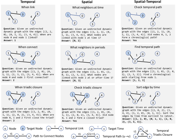
Figure 1: An overview of the tasks in the LLM4DyG Benchmark. The tasks are designed to consider both temporal and spatial dimensions, and question LLMs in natural language when, what or whether the spatial-temporal patterns take place. The spatial-temporal patterns range from temporal links, and chronological paths to dynamic triadic closure. The tasks are classified based on the targets of the queries. An example prompt and graph illustration are provided for each task.

2 Related Work

2.1 LLMs for tasks with graph data

Recently, there has been a surge of works about LLMs for solving tasks with graph data. He et al. (2023) proposed an approach that LLMs not only execute zero-shot predictions but also generate coherent explanations for their decisions. These explanations are subsequently leveraged to enhance the features of graph nodes for node classification in text-attributed graphs.  Chen et al. (2023b) proposes to explore LLMs-as-Enhancers and LLMs-as-Predictors for solving graph-related tasks, where the former augment the GNN with LLMs, and the latter directly adopts LLMs to make predictions. Wang et al. (2023a) introduced NLGraph, a benchmarking framework tailored for evaluating the performance of LLMs on traditional graph-related tasks. Simultaneously,  Guo et al. (2023) conducted a comprehensive empirical study focused on utilizing LLMs to tackle structural and semantic understanding tasks within graph-based contexts. Recent contributions in this line of research include InstructGLM (Ye et al., 2023), a method for fine-tuning LLMs inspired by LLaMA (Touvron et al., 2023), designed specifically for node classification tasks.  Zhang (2023) and  Jiang et al. (2023) have initiated the exploration of this frontier by interfacing LLMs with external tools and enhancing their reasoning capabilities over structured data sources such as knowledge graphs (KGs) and tables.  Pan et al. (2023) have provided a comprehensive roadmap for the seamless integration of LLMs with KGs, offering valuable insights into the potential synergies between language models and structured knowledge. However, these works mainly focus on static graphs, ignoring the temporal nature of graphs in real-world web applications. In this paper, we propose to explore LLMs on dynamic graphs, which remains unexplored in the literature.

2.2 LLMs for other related tasks

LLMs have been recently applied to other related tasks, including time-series forecasting, recommendation, etc.  Yu et al. (2023) presents a novel study on harnessing LLMs’ outstanding knowledge and reasoning abilities for explainable financial time series forecasting. Chang et al. (2023) leverages pre-trained LLMs to enhance time-series forecasting and has shown exceptional capabilities as both a robust representation learner and an effective few-shot learner.  Sun et al. (2023) summarizes two strategies for completing time-series (TS) tasks using LLM: LLM-for-TS that designs and trains a fundamental large model for TS data and TS-for-LLM that enables the pre-trained LLM to handle TS data.  Lyu et al. (2023) investigates various prompting strategies for enhancing personalized recommendation performance with large language models through input augmentation. However, these works do not consider the role of structures, and in this paper, we mainly focus on exploring the spatial-temporal understanding abilities of LLMs on dynamic graphs.

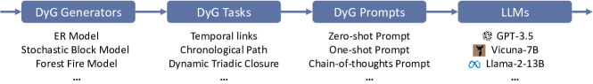
Figure 2: An overview of the pipeline in the LLM4DyG Benchmark, which includes various dynamic graph generators, tasks, prompt methods, and LLMs for evaluation.

2.3 Dynamic Graph Learning

Dynamic graphs are pervasive in a multitude of real-world applications, spanning areas such as event forecasting, recommendation systems, and many more (Cai et al., 2021; Deng et al., 2020; You et al., 2019; Wang et al., 2021b; Li et al., 2019; Wu et al., 2020; Zhang et al., 2022, 2023c, 2023b, 2023a). This prevalence has prompted significant research interest in the development and refinement of dynamic graph neural networks (Skarding et al., 2021; Zhu et al., 2022; Chen et al., 2023a). These networks are designed to model intricate graph dynamics, which incorporate evolving structures and features over time. A variety of approaches have been proposed to address the challenges posed by dynamic graphs. Some research efforts have focused on employing Graph Neural Networks (GNNs) to aggregate neighborhood information for each individual snapshot of the graph. Subsequently, these methods use a sequence module to capture and model the temporal information (Yang et al., 2021; Sun et al., 2021; Hajiramezanali et al., 2019; Seo et al., 2018; Sankar et al., 2020). In contrast, other studies have proposed the use of time-encoding techniques. These methods encode the temporal links into specific time-aware embeddings, and then utilize a GNN or memory module (Wang et al., 2021a; Cong et al., 2021; Xu et al., 2020; Rossi et al., 2020) to process and handle the structural information embedded in the graph. However, these methods require the model to be trained every time they encounter a new task, limiting their widespread usage. In this paper, we explore the potential of LLMs on dynamic graph tasks and evaluate their spatial-temporal understanding abilities.

3 The LLM4DyG Benchmark

In this section, we introduce our proposed LLM4DyG benchmark to evaluate whether LLMs are capable of understanding spatial-temporal information on the dynamic graph. Specifically, we first adopt a random dynamic graph generator to generate the base dynamic graphs with controllable parameters like time span. Then, we design nine dynamic graph tasks to evaluate LLMs’ abilities considering both spatial and temporal dimensions. The pipeline is illustrated in Figure 2. Based on this pipeline, we can control the data generation, statistics, prompting methods, and LLMs for each task to conduct fine-grained analyses.

3.1 Dynamic Graph Data Generators

We first adopt a random dynamic graph data generator to control the statistics of the dynamic graph. In default, we adopt an Erdős-Rényi (ER) model to generate an undirected graph, and randomly assign a time-stamp for each edge. Denote a graph $\mathcal{G}=(\mathcal{V},\mathcal{E})$ with the node set $\mathcal{V}=\{v_{1},v_{2},\dots v_{N}\}$ and edge set $\mathcal{E}=\{e_{1},e_{2},\dots,e_{M}\}$. We first generate the graph with the ER model $\mathcal{G}=ER(N,p)$ where $N$ is the number of nodes in the graph, and $p$ is the probability of edge occurrence between each node pair. In this way, $N$ controls the graph size, and $p$ controls the graph density. After obtaining the graph $\mathcal{G}$, we assign each edge with a random timestamp $t\sim U(\{0,1,\dots,T-1\})$, where $T$ controls the time span. For a generated dynamic graph, each edge $e=(v_{i},v_{j},t)$ denotes that node $v_{i}$ and node $v_{j}$ are linked at time $t$. We also include other dynamic graph generators, stochastic block (SB) model, and forest fire (FF) model.

3.2 Dynamic Graph Tasks

To evaluate LLMs’ spatial-temporal understanding abilities, we design nine tasks considering both temporal and spatial dimensions. The tasks are classified based on the targets of the queries, e.g., the temporal tasks make queries about the time, the spatial tasks make queries about the nodes, while the solutions in spatial-temporal tasks are more complex and include the spatial-temporal patterns mixed together. We introduce the definition and generation of each task as follows.

• Temporal Task 1: when link. We ask when two nodes are linked in this task. In a dynamic graph $\mathcal{G}=(\mathcal{V},\mathcal{E})$, two nodes $u$ and $v$ are linked at time $t$ if there exists a temporal edge $(u,v,t)$ in the edge set $\mathcal{E}$. We randomly select an edge from the edge set as the query.

• Temporal Task 2: when connect. We ask when two nodes are connected in this task. In a dynamic graph $\mathcal{G}=(\mathcal{V},\mathcal{E})$, two nodes $u$ and $v$ are connected at time $t$ if there exists a path $[(u,k_{1},t),(k_{1},k_{2},t),\dots,(k_{i},v,t)]$ from node $u$ to node $v$ at time $t$ in the edge set $\mathcal{E}$. We randomly select a pair of nodes that are connected at some time as the query.

• Temporal Task 3: when triadic closure (tclosure). We ask when the three given nodes first form a closed triad in this task. Dynamic triadic closure has been shown critical for dynamic graph analyses (Zhou et al., 2018). In a dynamic graph $\mathcal{G}=(\mathcal{V},\mathcal{E})$, two nodes with a common neighbor are said to have a triadic closure, if they are linked since some time so that the three nodes have linked with each other to form a triad. We randomly select a closed triad as the query.

Note that while these temporal tasks focus on making queries about time, they also require the model to understand structures so that the model can recognize when some structural patterns exist, from links and paths to dynamic triads. Next, we introduce the spatial tasks that require the model to spot the specific time and discover the structures.

• Spatial Task 1: what neighbor at time. In this task, we ask what nodes are linked with a given node at a given time. We randomly select a time and a node not isolated in the time-related graph snapshot to construct the query.

• Spatial Task 2: what neighbor in periods. In this task, we ask what nodes are linked with a given node after or at a given time, but not linked before the given time. We randomly select a time and a node not isolated before the given time to construct the query. This task measures the model’s abilities to understand structures within a time period, e.g., the latest links.

• Spatial Task 3: check triadic closure (tclosure). We ask whether the three given nodes form a closed triad in the dynamic graph through true/false questions. We uniformly sample from the sets of closed triads and open triads to construct the positive and negative samples respectively. We also keep a balanced number of positive and negative samples in the dataset.

Similarly, these tasks also require the model to spot the time, from a specific time and time period to the full-time span, and then to recognize what structural patterns or whether the given structural patterns meet the requirements of the queries. Next, we introduce the spatial-temporal tasks that directly require the LLMs to process the spatial-temporal targets.

• Spatial-Temporal Task 1: check temporal path (tpath). In this task, we ask whether the given three ordered nodes form a chronological path. In a dynamic graph $\mathcal{G}=(\mathcal{V},\mathcal{E})$, a sequence of nodes $[v_{1},v_{2},\dots,v_{n}]$ construct a chronological path if the timestamps of the edges do not decrease from source node $v_{1}$ to target node $v_{n}$ in the path. We randomly select positive and negative samples from the set of chronological paths and non-chronological paths to construct a balanced dataset.

• Spatial-Temporal Task 2: find temporal path (tpath). In this task, we ask the model to find a chronological path starting from a given node in the dynamic graph. We randomly select a node that is a starting node at any chronological path to construct the queries. Note that any valid chronological path starting at the given node is a correct answer.

• Spatial-Temporal Task 3: sort edge by time. In this task, we shuffle the edges and ask the model to sort the edges by time from earliest to latest. In the cases where some edges have the same timestamp, the orders within these edges do not matter for the correct answers.

These tasks require the model to understand the spatial-temporal information at the local or global scale. The targets of the queries include both temporal and spatial information on the dynamic graph. The example prompts and illustrations are shown in Fig. 1.

Table 1: An example of prompt construction for the ‘when connect’ task.

Prompt	Example
DyG Instruction	In an undirected dynamic graph, (u, v, t) means that node u and node v are linked with an undirected edge at time t.
Task Instruction	Your task is to answer when two nodes are first connected in the dynamic graph. Two nodes are connected if there exists a path between them.
Answer Instruction	Give the answer as an integer number at the last of your response after ’Answer:’
Exemplar	Here is an example: Question: Given an undirected dynamic graph with the edges [(0, 1, 0), (1, 2, 1), (0, 2, 2)]. When are node 0 and node 2 first connected? Answer:1
Question	Question: Given an undirected dynamic graph with the edges [(0, 9, 0), (1, 9, 0), (2, 5, 0), (1, 2, 1), (2, 6, 1), (3, 7, 1), (4, 5, 2), (4, 7, 2), (7, 8, 2), (0, 1, 3), (1, 6, 3), (5, 6, 3), (0, 4, 4), (3, 4, 4), (3, 6, 4), (4, 6, 4), (4, 9, 4), (6, 7, 4)]. When are node 2 and node 1 first connected?
Answer	Answer:1

4 Experiments

In this section, we conduct experiments to evaluate LLMs’ spatial-temporal understanding abilities on dynamic graphs. We conduct fine-grained analyses with various settings from different aspects, including data, prompting methods, models, etc.

4.1 Setups

Random baseline

To verify whether the model can understand dynamic graphs instead of outputting random answers, we adopt a random baseline that uniformly selects one of the possible solutions as the answer. The accuracies of the random baseline for the tasks can be calculated by the ratio of the number of correct solutions over the number of possible solutions, which are specifically provided as follows. For the tasks ‘when connect’ and ‘when tclosure’, the baseline accuracy is $\frac{1}{T}$. For the task ‘when link’, the baseline accuracy is $\frac{1}{\sum_{i}^{T}C(T,i)}$, where $C(T,i)$ is the combination number. For the tasks ‘neighbor at time’ and‘neighbor in periods’, the baseline accuracy is $\frac{1}{\sum_{i}^{N}C(N,i)}$. For the tasks ‘check tclosure’ and‘check tpath’, the baseline accuracies are 1/2, as the answer is either no or yes. For the tasks ‘find tpath’ and ‘check tpath’, the baseline accuracies are calculated by enumerating possible solutions and correct solutions for each instance.

Prompting methods

To investigate how different prompting techniques affect the model’s abilities, we compare various prompting methods, including zero-shot prompting, few-shot prompting (Brown et al., 2020), chain-of-thought prompting (COT) (Wei et al., 2022) and few-shot prompting with COT. We adopt one example for few-shot prompting, and use one-shot prompting as the default prompting approach. For each problem instance, the prompt is constructed by sequentially concatenating dynamic graph instruction, task instruction, answer instruction, exemplar prompts, and question prompts. An example of the prompt construction is shown in Table 1.

Models

We use GPT-3.5-turbo-instruct as the default LLM, and we also include other LLMs like Vicuna-7B, Vicuna-13B, Llama-2-13B and CodeLlama-2-13B. For all models, we set temperature $\tau=0$ for reproducibility. We adopt accuracy as the metric for all tasks.

Data

In default settings, we set $N=10$, $p=0.3$, $T=5$, and ER model for generating dynamic graphs. For each task and setting, we randomly generate one hundred problem instances for evaluation.

We run the experiments three times with different seeds, and report the average performance and their standard deviations.

Table 2: The overall model performance (ACC%) on the dynamic graph tasks. In the data column, ‘N’ denotes the number of nodes in the dynamic graph. In the model column, ‘Random’ denotes the random baseline which uniformly outputs one of the possible solutions, and ‘$\Delta$’ denotes the performance improvement of GPT-3.5 over the random baseline.

Task		Temporal			Spatial			Spatial-Temporal
Data	model	when link	when connect	when tclosure	neighbor at time	neighbor in periods	check tclosure	check tpath	find tpath	sort edge
N = 5	GPT-3.5	68.0$\pm$2.8	97.7$\pm$0.9	52.7$\pm$2.4	86.0$\pm$2.2	42.3$\pm$1.7	69.0$\pm$2.2	58.7$\pm$2.1	79.0$\pm$4.1	78.0$\pm$1.4
	Random	3.2	20.0	20.0	3.2	3.2	50.0	50.0	9.3	13.1
	$\Delta$	+64.8	+77.7	+32.7	+82.8	+39.1	+19.0	+8.7	+69.7	+64.9
N = 10	GPT-3.5	33.7$\pm$2.1	77.0$\pm$2.9	73.0$\pm$1.6	34.0$\pm$1.4	15.7$\pm$4.2	66.7$\pm$4.5	63.7$\pm$2.6	78.3$\pm$6.0	29.3$\pm$4.0
	Random	3.2	20.0	20.0	0.1	0.1	50.0	50.0	6.7	0.0
	$\Delta$	+30.4	+57.0	+53.0	+33.9	+15.6	+16.7	+13.7	+71.6	+29.3
N = 20	GPT-3.5	40.3$\pm$1.7	17.7$\pm$4.2	63.3$\pm$0.9	17.7$\pm$1.7	2.0$\pm$0.8	64.3$\pm$7.3	57.0$\pm$2.2	85.0$\pm$0.8	0.0$\pm$0.0
	Random	3.2	20.0	20.0	0.0	0.0	50.0	50.0	7.3	0.0
	$\Delta$	+37.1	-2.3	+43.3	+17.7	+2.0	+14.3	+7.0	+77.7	0.0
Avg.	GPT-3.5	47.3$\pm$1.2	64.1$\pm$0.3	63.0$\pm$1.0	45.9$\pm$3.1	20.0$\pm$0.8	66.7$\pm$2.9	59.8$\pm$0.8	80.8$\pm$0.3	35.8$\pm$2.0
	Random	3.2	20.0	20.0	1.1	1.1	50.0	50.0	7.8	4.4
	$\Delta$	+44.1	+44.1	+43.0	+44.8	+18.9	+16.7	+9.8	+73.0	+31.4

4.2 Results with data of different statistics

We first compare GPT-3.5 on each task with different graph sizes, where $N$ is set to 5, 10 and 20 respectively. From Table 2, we have the following observations.

Observation 1. LLMs have preliminary spatial-temporal understanding abilities on dynamic graphs.

As shown in Table 2, on average, GPT-3.5 has shown significant performance improvement (from +9.8% to +73.0%) over the baseline for all tasks, indicating that LLMs indeed understand the dynamic graph as well as the question in the task, and are able to exploit spatial-temporal information to give correct answers instead of guessing by outputting randomly generated answers. Overall, we can find that LLMs have the ability to recognize time, structures, and spatial-temporal patterns.

Observation 2. Most dynamic graph tasks exhibit increasing difficulty for LLMs as the graph size grows.

As shown in Table 2, for most tasks, the performance of GPT-3.5 drops as the graph size $N$ increases. For example, the performance drops from 97.7% to 17.7% on ‘when connect’ task, and 42.3% to 2.0% on ‘neighbor in periods’ task. This phenomenon may be due to two factors: 1) From the task perspective, the solution space is enlarged so that it is harder for any model to obtain the correct solution, e.g., the accuracy of the random baseline also drops significantly on ‘sort edge’ task. 2) From the model perspective, it is harder for the model to retrieve the useful information inside the data since the input space is enlarged, e.g., on ‘when connect’ task, the performance drops drastically while the solution space remains the same. This observation shows that it is worthy of exploring handling larger dynamic graph contexts with LLMs.

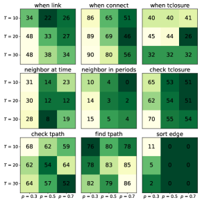
Figure 3: Performance comparisons (ACC%) on the dynamic graph tasks with different density $p$ and time span $T$. (Best viewed in color)

We then compare GPT-3.5 on each task with different time span $T$ and density $p$, where $T$ is set to 10, 20, and 30 respectively, and $p$ is set to 0.3, 0.5, and 0.7 respectively. From Figure 3, we have the following observations.

Observation 3. For LLMs, the difficulties of dynamic graph tasks are not sensitive to the time span but sensitive to the graph density.

As shown in Figure 3, for most tasks, the model performance is close as the time span $T$ increases while the density $p$ remains the same. If we keep the time span $T$ the same and increase the density $p$, the model performance drops for most tasks. One exception is the task ‘find tpath’ where the model performance increases as the two factors increase. Another interesting finding from the heatmap is that LLMs are relatively more sensitive with the time span $T$ in temporal tasks while the density $p$ in spatial tasks, possibly due to the different points of focus for these tasks. It can be also observed in spatial-temporal tasks, where the model performance mainly changes along with the diagonal of the time span $T$ and density $p$.

To investigate how the performance of LLMs varies when the task requires additional temporal information other than only structural information, we make comparisons with different time span $T$ and graph size $N$ on the ‘neighbor at time’ task. We have the following observation.

Table 3: Performance comparisons (ACC%) of various prompting methods on the dynamic graph tasks. ‘Random’ denotes the random baseline which uniformly outputs one of the possible solutions. The best result for each task is in bold.

Task	Temporal			Spatial			Spatial-Temporal
Prompt Method	when link	when connect	when tclosure	neighbor at time	neighbor in periods	check tclosure	check tpath	find tpath	sort edge
zero-shot	2.3$\pm$0.5	73.3$\pm$2.1	68.0$\pm$0.8	36.0$\pm$4.3	4.3$\pm$2.1	70.7$\pm$1.7	66.0$\pm$5.4	56.3$\pm$9.0	33.7$\pm$7.4
one-shot	33.7$\pm$2.1	77.0$\pm$2.9	73.0$\pm$1.6	34.0$\pm$1.4	15.7$\pm$4.2	66.7$\pm$4.5	63.7$\pm$2.6	78.3$\pm$6.0	29.3$\pm$4.0
zero-shot COT	1.0$\pm$0.8	58.3$\pm$1.2	70.0$\pm$1.6	32.0$\pm$0.8	4.3$\pm$2.6	55.0$\pm$1.4	62.3$\pm$2.9	58.0$\pm$9.1	44.7$\pm$0.5
one-shot COT	10.3$\pm$0.5	76.0$\pm$2.4	80.0$\pm$1.6	27.7$\pm$1.9	13.0$\pm$3.6	57.7$\pm$2.1	57.7$\pm$3.4	81.3$\pm$2.6	24.7$\pm$2.4

Observation 4. Temporal information adds additional difficulties to LLMs in comparisons with static graphs.

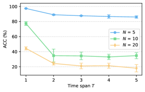
Figure 4: Performance of GPT-3.5 on the ‘neighbor at time’ task as the time span $T$ increases with different network sizes $N$. Note that when $T=1$, the data degenerates to a static graph, since there is only one timestamp on the graph.

As shown in Figure 4, GPT-3.5 has a drastic performance drop when the time span $T$ increases from 1 to 2. The possible reason is that the task is changed from static to dynamic, serving as a more challenging setting, since the model has to capture the additional temporal information. Similar to the results from Figure 3, the model performance is not sensitive to the time span when the task is already a dynamic graph problem.

4.3 Results with different prompting methods

We then make comparisons with different prompting methods, including zero-shot prompting, one-shot prompting, zero-shot chain-of-thoughts, and one-shot chain-of-thoughts. From Tab. 3, we have the following observations.

Observation 5. General advanced prompting techniques do not guarantee a performance boost in tackling spatial-temporal information.

As shown in Table 3, some advanced prompting methods like zero-shot COT and one-shot COT achieve higher performance than other prompting methods in the tasks ‘when tclosure’, ‘find tpath’ and ‘sort edge’. Note that these tasks involve more complex dynamic graph concepts or have to tackle a large time span, which shows that the chain-of-thoughts method can, to some extent, activate the model’s reasoning ability by thinking step by step on complex tasks. However, no prompting methods consistently achieve the best performance on all tasks, which calls for the need to design special advanced prompting methods to boost LLMs’ performance in handling spatial-temporal information on dynamic graphs.

4.4 Results with different LLMs

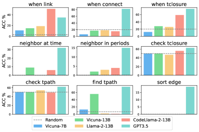
Figure 5: Performance comparisons (ACC%) of various LLMs on the dynamic graph tasks. ‘Random’ denotes the random baseline which uniformly outputs one of the possible solutions. (Best viewed in color)

Table 4: Valid rate (%) of different LLMs. An answer is judged as valid if it meets the requirement of the answer template and can be parsed by the evaluator program.

Valid Rate when link when connect when tclosure neighbor at time neighbor in periods sort edge Vicuna-7B 100 100 100 100 99 10 Vicuna-13B 92 89 100 93 97 92 Llama-2-13B 99 97 95 21 91 74 CodeLlama-2-13B 100 100 100 100 96 100 GPT-3.5 100 100 100 100 100 100

Table 5: Performance comparisons (ACC%) of various prompting methods and dynamic graph generation models on the ‘when link’ task.

Generation Model	ER Model	SB Model	FF Model
zero-shot	2.3$\pm$0.5	7.7$\pm$1.7	5.3$\pm$2.5
one-shot	33.7$\pm$2.1	46.0$\pm$2.9	48.0$\pm$7.1
zero-shot COT	1.0$\pm$0.8	5.7$\pm$3.1	2.0$\pm$1.6
one-shot COT	10.3$\pm$0.5	15.3$\pm$0.9	13.0$\pm$2.9

Table 6: Model performance (ACC%) on the dynamic graph tasks with one-shot prompting method and our proposed DST2 prompting methods (v1 to v4). The best and the second-best results for each task are in bold and underlined respectively.

Task Temporal Spatial Spatial-Temporal Prompting methods when link when connect when tclosure neighbor at time neighbor in periods check tclosure check tpath find tpath sort edge one-shot prompt 33.7$\pm$2.1 77.0$\pm$2.9 73.0$\pm$1.6 34.0$\pm$1.4 15.7$\pm$4.2 66.7$\pm$4.5 63.7$\pm$2.6 78.3$\pm$6.0 29.3$\pm$4.0 v1: Think (about) nodes and then time 40.0$\pm$1.6 77.0$\pm$4.1 74.0$\pm$1.4 34.0$\pm$0.8 15.0$\pm$4.2 69.3$\pm$1.7 61.0$\pm$3.3 79.0$\pm$7.5 30.0$\pm$3.6 v2: Think (about) time and then nodes 37.3$\pm$2.6 76.7$\pm$3.4 73.3$\pm$0.5 31.7$\pm$1.9 15.7$\pm$3.4 67.0$\pm$2.9 61.3$\pm$1.9 79.0$\pm$7.5 30.7$\pm$3.9 v3: Pick nodes and then time 59.3$\pm$2.1 77.0$\pm$2.4 68.0$\pm$0.8 35.0$\pm$2.9 16.7$\pm$4.7 65.0$\pm$3.7 62.3$\pm$2.9 78.0$\pm$5.4 30.0$\pm$2.9 v4: Pick time and then nodes 76.7$\pm$1.7 76.3$\pm$3.9 68.7$\pm$0.9 35.7$\pm$2.5 15.3$\pm$3.3 65.3$\pm$2.9 63.3$\pm$2.6 78.3$\pm$5.8 29.3$\pm$2.9

We then make comparisons with different LLMs, including GPT-3.5, Llama-2-13B, Vicuna-7B, Vicuna-13B and CodeLlama-2-13B. From Figure 5, we have the following observations.

Observation 6. LLMs’ abilities on dynamic graph tasks are related to the model scale.

As shown in Figure 5, smaller LLMs like vicuna-7B and Llama-2-13B have performance lower than GPT-3.5 for all tasks, and even lower than random baseline for several tasks like ‘when connect’ and ‘check tclosure’. Overall, for these tasks, larger LLMs have better performance.

To further investigate whether the lower performance stems from the incompetence of understanding instructions or performing reasoning, we show the valid rate of the answers given by different LLMs in several tasks. An answer is judged as valid if it meets the requirement of the answer template and can be parsed by the evaluator program. From Table 4, we find that 1) smaller models have significantly lower valid rates for some tasks, e.g., 21% of Llama-2-13B in the task ‘neighbor at time’, demonstrating their limitations in understanding human instructions for dynamic graph tasks. 2) In some tasks, the smaller models have high valid rates, while having significantly lower performance than GPT-3.5, showing their limitations in reasoning for dynamic graph tasks.

Observation 7. Training on codes may help LLMs tackle on dynamic graph tasks.

As shown in Figure 5, compared with Llama-2-13B, CodeLlama-2-13B shows significantly better results in most tasks. In particular, CodeLlama-2-13B even outperforms GPT-3.5 in the task ‘when link’. Note that in comparison with Llama-2-13B, CodeLlama-2-13B is further pretrained on a large corpus of code data, which shows the potential of improving the performance of LLMs on dynamic graph tasks by training with codes. One possible reason is that the code data covers more implicit knowledge of structures and sequences, e.g., the control flows of the programs and their comments as explanations, which might be useful for LLMs to understand dynamic graphs.

4.5 Results with different data generators

We make comparisons with various prompting methods and dynamic graph generation models, including Erdős–Rényi (ER) model, Stochastic Block (SB) model, and Forest Fire (FF) model, on the ‘when link’ task. To keep the number of edges similar, we set the class number as 2, the in-class probability as 0.4, the cross-class probability as 0.2 for SB model, and the forward burning probability as 0.5 for FF model.

Observation 8. General prompting methods have consistent performance with different dynamic graph generators in the same task.

As shown in Table 5, the ‘one-shot’ prompt method consistently achieves the best performance with different dynamic graph generation models in the ‘when link’ task. The results indicate that the evaluation of different prompting methods on dynamic graphs may not be closely related to the dynamic graph generators.

4.6 Exploring advanced dynamic graph prompts

In this section, we aim to explore advanced dynamic graph prompting techniques to improve the reasoning ability of LLMs on dynamic graphs. The chain-of-thoughts prompting is shown as a general advanced prompting technique to activate LLMs’ complex reasoning abilities, while it does not effectively improve performance on dynamic graphs as shown in Table 3.

To have further developments, we draw inspiration from dynamic graph learning literature where most works tackle spatial-temporal information separately, e.g., to tackle time first and then structures, or to tackle structures first and then time. Intuitively, this thought breaks down the complex spatial-temporal information into two separate dimensions so that the difficulty can be decreased. To this end, we propose Disentangled Spatial-Temporal Thoughts (DST2) to improve LLMs’ reasoning abilities on dynamic graphs, that is to instruct LLMs to sequentially think about the nodes or time. Specifically, we design several prompts and add the prompts after the task instruction in the one-shot prompt, which are denoted as ‘v1’ to ‘v4’ respectively in Table 6.

Observation 9. The prompting of instructing LLMs to separately tackle spatial and temporal information significantly improves the performance.

As shown in Table 6, the prompt ‘v4’ achieves the accuracy of 76.7% in the ‘when link’ task, significantly surpassing the one-shot prompt (33.7%), showing that guiding the LLM to handle time before nodes may help the model improve the spatio-temporal understanding ability on dynamic graphs. For spatial tasks, it seems that it would be better for the LLM to think about spatial information before temporal information ( e.g., the prompt ‘v1’ achieves 69.3% in the ‘check tclosure’ task). While our proposed methods provide performance gains in most tasks, there exist some tasks that are not positively affected. Designing specific prompting methods for LLMs on dynamic graphs is still an open research question.

5 Conclusion

In this paper, we propose a novel LLM4DyG benchmark to evaluate LLMs’ spatial-temporal understanding capabilities on dynamic graphs, which remains unexplored in literature. The proposed benchmark encompasses nine specially devised tasks, which assess the capabilities of LLMs to handle both temporal and spatial information on dynamic graphs. The evaluation procedure involves a diverse range of LLMs, prompting techniques, data generators, and data statistics. We also propose Disentanlged Spatio-Temporal Thoughts (DST2) as an advanced prompting method to enhance reasoning capabilities by guiding LLMs to think about time and structures separately. Through comprehensive experiments, we provide nine fine-grained observations that would be helpful for understanding LLMs’ reasoning abilities on dynamic graphs. We hope that future work can be developed based on our proposed benchmark and observations.

References

- Alayrac et al. (2022) Alayrac, J.-B., Donahue, J., Luc, P., Miech, A., Barr, I., Hasson, Y., Lenc, K., Mensch, A., Millican, K., Reynolds, M., et al. Flamingo: a visual language model for few-shot learning. Advances in Neural Information Processing Systems, 35:23716–23736, 2022.
- Brown et al. (2020) Brown, T., Mann, B., Ryder, N., Subbiah, M., Kaplan, J. D., Dhariwal, P., Neelakantan, A., Shyam, P., Sastry, G., Askell, A., Agarwal, S., Herbert-Voss, A., Krueger, G., Henighan, T., Child, R., Ramesh, A., Ziegler, D., Wu, J., Winter, C., Hesse, C., Chen, M., Sigler, E., Litwin, M., Gray, S., Chess, B., Clark, J., Berner, C., McCandlish, S., Radford, A., Sutskever, I., and Amodei, D. Language models are few-shot learners. In Advances in Neural Information Processing Systems, pp. 1877–1901, 2020.
- Cai et al. (2021) Cai, L., Chen, Z., Luo, C., Gui, J., Ni, J., Li, D., and Chen, H. Structural temporal graph neural networks for anomaly detection in dynamic graphs. In Proceedings of the 30th ACM international conference on Information & Knowledge Management, pp. 3747–3756, 2021.
- Chang et al. (2023) Chang, C., Peng, W.-C., and Chen, T.-F. Llm4ts: Two-stage fine-tuning for time-series forecasting with pre-trained llms. arXiv preprint arXiv:2308.08469, 2023.
- Chen et al. (2023a) Chen, C., Geng, H., Yang, N., Yang, X., and Yan, J. Easydgl: Encode, train and interpret for continuous-time dynamic graph learning. arXiv preprint arXiv:2303.12341, 2023a.
- Chen et al. (2023b) Chen, Z., Mao, H., Li, H., Jin, W., Wen, H., Wei, X., Wang, S., Yin, D., Fan, W., Liu, H., and Tang, J. Exploring the potential of large language models (llms) in learning on graphs. arXiv preprint arXiv:2307.03393, 2023b.
- Chiang et al. (2023) Chiang, W.-L., Li, Z., Lin, Z., Sheng, Y., Wu, Z., Zhang, H., Zheng, L., Zhuang, S., Zhuang, Y., Gonzalez, J. E., Stoica, I., and Xing, E. P. Vicuna: An open-source chatbot impressing gpt-4 with 90%* chatgpt quality, March 2023. URL https://lmsys.org/blog/2023-03-30-vicuna/.
- Cong et al. (2021) Cong, W., Wu, Y., Tian, Y., Gu, M., Xia, Y., Mahdavi, M., and Chen, C.-c. J. Dynamic graph representation learning via graph transformer networks. arXiv preprint arXiv:2111.10447, 2021.
- Deng et al. (2020) Deng, S., Rangwala, H., and Ning, Y. Dynamic knowledge graph based multi-event forecasting. In Proceedings of the 26th ACM SIGKDD International Conference on Knowledge Discovery & Data Mining, pp. 1585–1595, 2020.
- Erdős et al. (1960) Erdős, P., Rényi, A., et al. On the evolution of random graphs. Publ. math. inst. hung. acad. sci, 5(1):17–60, 1960.
- Guo et al. (2023) Guo, J., Du, L., and Liu, H. Gpt4graph: Can large language models understand graph structured data? an empirical evaluation and benchmarking. arXiv preprint arXiv:2305.15066, 2023.
- Hajiramezanali et al. (2019) Hajiramezanali, E., Hasanzadeh, A., Narayanan, K., Duffield, N., Zhou, M., and Qian, X. Variational graph recurrent neural networks. Advances in neural information processing systems, 32, 2019.
- He et al. (2023) He, X., Bresson, X., Laurent, T., and Hooi, B. Explanations as features: Llm-based features for text-attributed graphs. arXiv preprint arXiv:2305.19523, 2023.
- Holland et al. (1983) Holland, P. W., Laskey, K. B., and Leinhardt, S. Stochastic blockmodels: First steps. Social networks, 5(2):109–137, 1983.
- Jiang et al. (2023) Jiang, J., Zhou, K., Dong, Z., Ye, K., Zhao, W. X., and Wen, J.-R. Structgpt: A general framework for large language model to reason over structured data. arXiv preprint arXiv:2305.09645, 2023.
- Leskovec et al. (2007) Leskovec, J., Kleinberg, J., and Faloutsos, C. Graph evolution: Densification and shrinking diameters. ACM transactions on Knowledge Discovery from Data (TKDD), 1(1):2–es, 2007.
- Li et al. (2019) Li, H., Cui, P., Zang, C., Zhang, T., Zhu, W., and Lin, Y. Fates of microscopic social ecosystems: Keep alive or dead? In Proceedings of the 25th ACM SIGKDD International Conference on Knowledge Discovery & Data Mining, pp. 668–676, 2019.
- Lyu et al. (2023) Lyu, H., Jiang, S., Zeng, H., Xia, Y., and Luo, J. Llm-rec: Personalized recommendation via prompting large language models. arXiv preprint arXiv:2307.15780, 2023.
- Pan et al. (2023) Pan, S., Luo, L., Wang, Y., Chen, C., Wang, J., and Wu, X. Unifying large language models and knowledge graphs: A roadmap. arXiv preprint arXiv:2306.08302, 2023.
- Rossi et al. (2020) Rossi, E., Chamberlain, B., Frasca, F., Eynard, D., Monti, F., and Bronstein, M. Temporal graph networks for deep learning on dynamic graphs. arXiv preprint arXiv:2006.10637, 2020.
- Rozière et al. (2023) Rozière, B., Gehring, J., Gloeckle, F., Sootla, S., Gat, I., Tan, X. E., Adi, Y., Liu, J., Remez, T., Rapin, J., Kozhevnikov, A., Evtimov, I., Bitton, J., Bhatt, M., Ferrer, C. C., Grattafiori, A., Xiong, W., Défossez, A., Copet, J., Azhar, F., Touvron, H., Martin, L., Usunier, N., Scialom, T., and Synnaeve, G. Code llama: Open foundation models for code, 2023.
- Sankar et al. (2020) Sankar, A., Wu, Y., Gou, L., Zhang, W., and Yang, H. Dysat: Deep neural representation learning on dynamic graphs via self-attention networks. In Proceedings of the 13th International Conference on Web Search and Data Mining, pp. 519–527, 2020.
- Seo et al. (2018) Seo, Y., Defferrard, M., Vandergheynst, P., and Bresson, X. Structured sequence modeling with graph convolutional recurrent networks. In International Conference on Neural Information Processing, pp. 362–373. Springer, 2018.
- Skarding et al. (2021) Skarding, J., Gabrys, B., and Musial, K. Foundations and modeling of dynamic networks using dynamic graph neural networks: A survey. IEEE Access, 9:79143–79168, 2021.
- Sun et al. (2023) Sun, C., Li, Y., Li, H., and Hong, S. Test: Text prototype aligned embedding to activate llm’s ability for time series. arXiv preprint arXiv:2308.08241, 2023.
- Sun et al. (2021) Sun, L., Zhang, Z., Zhang, J., Wang, F., Peng, H., Su, S., and Yu, P. S. Hyperbolic variational graph neural network for modeling dynamic graphs. In Proceedings of the AAAI Conference on Artificial Intelligence, volume 35, pp. 4375–4383, 2021.
- Thirunavukarasu et al. (2023) Thirunavukarasu, A. J., Ting, D. S. J., Elangovan, K., Gutierrez, L., Tan, T. F., and Ting, D. S. W. Large language models in medicine. Nature medicine, 29(8):1930–1940, 2023.
- Touvron et al. (2023) Touvron, H., Lavril, T., Izacard, G., Martinet, X., Lachaux, M.-A., Lacroix, T., Rozière, B., Goyal, N., Hambro, E., Azhar, F., et al. Llama: Open and efficient foundation language models. arXiv preprint arXiv:2302.13971, 2023.
- Wang et al. (2023a) Wang, H., Feng, S., He, T., Tan, Z., Han, X., and Tsvetkov, Y. Can language models solve graph problems in natural language? arXiv preprint arXiv:2305.10037, 2023a.
- Wang et al. (2023b) Wang, L., Ma, C., Feng, X., Zhang, Z., Yang, H., Zhang, J., Chen, Z., Tang, J., Chen, X., Lin, Y., et al. A survey on large language model based autonomous agents. arXiv preprint arXiv:2308.11432, 2023b.
- Wang et al. (2021a) Wang, Y., Chang, Y.-Y., Liu, Y., Leskovec, J., and Li, P. Inductive representation learning in temporal networks via causal anonymous walks. arXiv preprint arXiv:2101.05974, 2021a.
- Wang et al. (2021b) Wang, Y., Li, P., Bai, C., and Leskovec, J. Tedic: Neural modeling of behavioral patterns in dynamic social interaction networks. In Proceedings of the Web Conference 2021, pp. 693–705, 2021b.
- Wei et al. (2022) Wei, J., Wang, X., Schuurmans, D., Bosma, M., Xia, F., Chi, E., Le, Q. V., Zhou, D., et al. Chain-of-thought prompting elicits reasoning in large language models. Advances in Neural Information Processing Systems, 35:24824–24837, 2022.
- Wu et al. (2020) Wu, J., Cao, M., Cheung, J. C. K., and Hamilton, W. L. Temp: Temporal message passing for temporal knowledge graph completion. arXiv preprint arXiv:2010.03526, 2020.
- Xu et al. (2020) Xu, D., Ruan, C., Korpeoglu, E., Kumar, S., and Achan, K. Inductive representation learning on temporal graphs. arXiv preprint arXiv:2002.07962, 2020.
- Yang et al. (2021) Yang, M., Zhou, M., Kalander, M., Huang, Z., and King, I. Discrete-time temporal network embedding via implicit hierarchical learning in hyperbolic space. In Proceedings of the 27th ACM SIGKDD Conference on Knowledge Discovery & Data Mining, pp. 1975–1985, 2021.
- Ye et al. (2023) Ye, R., Zhang, C., Wang, R., Xu, S., and Zhang, Y. Natural language is all a graph needs. arXiv preprint arXiv:2308.07134, 2023.
- You et al. (2019) You, J., Wang, Y., Pal, A., Eksombatchai, P., Rosenburg, C., and Leskovec, J. Hierarchical temporal convolutional networks for dynamic recommender systems. In The world wide web conference, pp. 2236–2246, 2019.
- Yu et al. (2023) Yu, X., Chen, Z., Ling, Y., Dong, S., Liu, Z., and Lu, Y. Temporal data meets llm–explainable financial time series forecasting. arXiv preprint arXiv:2306.11025, 2023.
- Zhang (2023) Zhang, J. Graph-toolformer: To empower llms with graph reasoning ability via prompt augmented by chatgpt. arXiv preprint arXiv:2304.11116, 2023.
- Zhang et al. (2022) Zhang, Z., Wang, X., Zhang, Z., Li, H., Qin, Z., and Zhu, W. Dynamic graph neural networks under spatio-temporal distribution shift. In Advances in Neural Information Processing Systems, 2022.
- Zhang et al. (2023a) Zhang, Z., Li, X., Teng, F., Lin, N., Zhu, X., Wang, X., and Zhu, W. Out-of-distribution generalized dynamic graph neural network for human albumin prediction. In IEEE International Conference on Medical Artificial Intelligence, 2023a.
- Zhang et al. (2023b) Zhang, Z., Wang, X., Zhang, Z., Qin, Z., Wen, W., Xue, H., Li, H., and Zhu, W. Spectral invariant learning for dynamic graphs under distribution shifts. In Advances in Neural Information Processing Systems, 2023b.
- Zhang et al. (2023c) Zhang, Z., Zhang, Z., Wang, X., Qin, Y., Qin, Z., and Zhu, W. Dynamic heterogeneous graph attention neural architecture search. In Thirty-Seventh AAAI Conference on Artificial Intelligence, 2023c.
- Zhou et al. (2018) Zhou, L., Yang, Y., Ren, X., Wu, F., and Zhuang, Y. Dynamic network embedding by modeling triadic closure process. In Proceedings of the AAAI conference on artificial intelligence, volume 32, 2018.
- Zhu et al. (2022) Zhu, Y., Lyu, F., Hu, C., Chen, X., and Liu, X. Learnable encoder-decoder architecture for dynamic graph: A survey. arXiv preprint arXiv:2203.10480, 2022.