Invariant Physics-Informed Neural Networks for Ordinary Differential Equations

Abstract

Physics-informed neural networks have emerged as a prominent new method for solving differential equations. While conceptually straightforward, they often suffer training difficulties that lead to relatively large discretization errors or the failure to obtain correct solutions. In this paper we introduce invariant physics-informed neural networks for ordinary differential equations that admit a finite-dimensional group of Lie point symmetries. Using the method of equivariant moving frames, a differential equation is invariantized to obtain a, generally, simpler equation in the space of differential invariants. A solution to the invariantized equation is then mapped back to a solution of the original differential equation by solving the reconstruction equations for the left moving frame. The invariantized differential equation together with the reconstruction equations are solved using a physcis-informed neural network, and form what we call an invariant physics-informed neural network. We illustrate the method with several examples, all of which considerably outperform standard non-invariant physics-informed neural networks.

1 Introduction

Physics-informed neural networks (PINN) are an emerging method for solving differential equations using deep learning, [23, 30]. The main idea behind this method is to train a neural network as an approximate solution interpolant for a system of differential equations. This is done by minimizing a loss function that incorporates both the differential equations and any associated initial and/or boundary conditions. The method has a particular elegance as the derivatives in the differential equations can be computed using automatic differentiation rather than numerical discretization, which greatly simplifies the solution procedure, especially when solving differential equations on arbitrary surfaces, [35].

The ease of the discretization procedure in physics-informed neural networks, however, comes at the price of numerous training difficulties, and numerical solutions that are either not particularly accurate, or fail to converge at all to the true solution of the given differential equation. Since training a physics-informed neural network constitutes a non-convex optimization problem, an analysis of failure modes when physics-informed neural networks fail to train accurately is a non-trivial endeavour. This is why several modified training methodologies have been proposed, which include domain decomposition strategies, [18], modified loss functions, [38], and custom optimization, [3]. While all of these strategies, sometimes substantially, improve upon vanilla physics-informed neural networks, none of these modified approaches completely overcome all the inherent training difficulties.

Here we propose a new approach for training physics-informed neural networks, which relies on using Lie point symmetries of differential equations and the method of equivariant moving frames to simplify the form of the differential equations that have to be solved. This is accomplished by first projecting the differential equation onto the space of differential invariant to produce an invariantized differential equation. The solution to the invariantized equation is then mapped back to the solution of the original equation by solving a system of first order differential equations for the left moving frame, called reconstruction equations. The invariant physics-informed neural network architecture proposed in this paper consists of simultaneously solving the system of equations consisting of the invariantized differential equation and the reconstruction equations using a physics-informed neural network. The method proposed is entirely algorithmic, and can be implemented for any system of differential equations that is strongly invariant under the action of a group of Lie point symmetries. Since almost all equations of physical relevance admit a non-trivial group of Lie point symmetries, the proposed method is potentially a viable path for improving physics-informed neural networks for many real-world applications. The idea of projecting a differential equation into the space of invariants and then reconstructing its solution is reminiscent of the recent work [37], where the authors consider Hamiltonian systems with symmetries, although the tools used in our paper and in [37] to achieve the desired goals are very different. Moreover, in our approach we do not assume that our equations have an underlying symplectic structure.

To simplify the theoretical exposition, we focus on the case of ordinary differential equations in this paper. We show using several examples that the proposed approach substantially improves upon the numerical results achievable with vanilla physics-informed neural networks. Applications to partial differential equations will be considered elsewhere.

The paper is organized as follows. We first review relevant work on physics-informed neural networks and symmetry preserving numerical methods in Section 2. In Section 3 we introduce the methods of equivariant moving frames and review how it can be used to solve ordinary differential equations that admit a group of Lie point symmetries. Building on Section 3 we introduce a version of invariant physics-informed neural network in Section 4. We illustrate our method with several examples in Section 5. The examples show that our proposed invariant physics-informed neural network formulation can yield better numerical results than its non-invariant version. A short summary and discussion about potential future research avenues concludes the paper in Section 6.

2 Previous work

Physics-informed neural networks were first proposed in [23], and later popularized through the work of Raissi et al., [30]. The main idea behind physics-informed neural networks is to train a deep neural network to directly approximate the solution to a system of differential equations. This is done by defining a loss function that incorporates the given system of equations, along with any relevant initial and/or boundary conditions. Crucially, this turns training physics-informed neural networks into a multi-task, non-convex optimization problem that can be challenging to minimize, [22]. There have been several solutions proposed to overcome the training difficulties and improve the generalization capabilities of physics-informed neural networks. These include modified loss functions, [26, 38], meta-learned optimization, [3], domain decomposition methods, [6, 18], and the use of operator-based methods, [11, 24].

The concepts of symmetries and transformation groups have also received considerable attention in the machine learning community. Notably, the equivariance of convolutional operations with respect to spatial translations has been identified as a crucial ingredient for the success of convolutional neural networks, [13]. The generalization of this observation for other types of layers of neural networks and other transformation groups has become a prolific subfield of deep learning since. For example, see [16] for some recent results.

Here we do not consider the problem of endowing a neural network with equivariance properties but rather investigate the question whether a better formulation of a given differential equation can help physics-informed neural networks better learn a solution. As we will be using symmetries of differential equations for this re-formulation, our approach falls within the framework of geometric numerical integration. The problem of symmetry-preserving numerical schemes, in other words the problem of designing discretization methods for differential equations that preserve the symmetries of a given differential equation, has been studied extensively over the past several decades, see [14, 34, 39] for some early work on the topic. Invariant discretization schemes have since been proposed for finite difference, finite volume, finite elements and meshless methods, [2, 4, 5, 7, 8, 12, 19, 28, 31, 32].

3 Method

In this section we introduce the theoretical foundations on which the invariant physics-informed neural network framework is based. In order to fix some notation, we begin by recalling certain well-known results pertaining to symmetries of differential equations, and refer the reader to [9, 10, 17, 27] for a more thorough exposition. Within this field, the use of moving frames to solve differential equations admitting symmetries is not as well-known. Therefore, the main purpose of this section is to introduce this solution procedure. In contrast to the approach proposed in [25], we avoid the introduction of computational variables. All computations are based on the differential invariants of the prolonged group action which results in less differential equations. Our approach is a simplified version of the algorithm presented in [36], which deals with partial differential equations admitting infinite-dimensional symmetry Lie pseudo-groups.

As mentioned in the introduction, in this paper we limit ourselves to the case of ordinary differential equations.

3.1 Invariant differential equations

Let $M$ be a $(q+1)$-dimensional manifold with $q\geq 1$. Given a one-dimensional curve $C\subset M$, we introduce the local coordinates $z=(t,u)=(t,u^{1},\ldots,u^{q})$ on $M$ so that the curve $C$ is locally specified by the graph of a function $C=\{(t,f(t))\}$. Accordingly, the $n$-th order jet space $\mathrm{J}^{(n)}$ is locally parametrized by $z^{(n)}=(t,u^{(n)})$, where $u^{(n)}$ denotes all the derivatives $u^{\alpha}_{j}=u^{\alpha}_{t^{j}}$ of order $0\leq j\leq n$, with $\alpha=1,\ldots,q$.

Let $G$ be an $r$-dimensional Lie group (locally) acting on $M$:

$$(T,U)=Z=g\cdot z=g\cdot(t,u),\qquad\text{where}\qquad g\in G.$$ (1)

The group transformation (1) induces an action on curves $C\subset M$, which prolongs to the jet space $\mathrm{J}^{(n)}$:

$$Z^{(n)}=g\cdot z^{(n)}.$$ (2)

Coordinate expressions for the prolonged action (2) are obtained by applying the implicit total derivative operator

$$\mathrm{D}_{T}=\frac{1}{\text{D}_{t}(T)}\,\mathrm{D}_{t},\qquad\text{where}\qquad\mathrm{D}_{t}=\frac{\partial}{\partial t}+\sum_{j=0}^{\infty}\sum_{\alpha=1}^{q}\>u^{\alpha}_{j+1}\frac{\partial}{\partial u^{\alpha}_{j}}$$

denotes the standard total derivative operator, to the transformed dependent variables $U^{\alpha}$:

$$U^{\alpha}_{j}=U^{\alpha}_{T^{j}}=\mathrm{D}_{T}^{j}(U^{\alpha}),\qquad\alpha=1,\ldots,q,\qquad j\geq 0.$$ (3)

In the following we use the notation $\Delta(z^{(n)})=\Delta(t,u^{(n)})=0$ to denote a system of differential equations, and use the index notation $\Delta_{i}(z^{(n)})=0$, $i=1,\ldots,l,$ to label each equation in $\Delta(z^{(n)})$. Also, a differential equation $\Delta(z^{(n)})=0$, can either be a single equation or represent a system of differential equations.

Definition 1.

A nondegenerate ordinary differential equation $\Delta(z^{(n)})=0$ is said to be strongly invariant under the prolonged action of a connected local Lie group of transformations $G$ if and only if

$$\Delta(g\cdot z^{(n)})=0\qquad\text{for all}\qquad g\in G$$

near the identity element.

Remark 2.

Strong invariance is more restrictive than the usual notion of symmetry, where invariance is only required to hold on the solution space. In the following, we require strong invariance to guarantee that our differential equation is an invariant function.

Invariance is usually stated in terms of the infinitesimal generators of the group action. To this end, let

$$\mathbf{v}_{\kappa}=\xi_{\kappa}(t,u)\frac{\partial}{\partial t}+\sum_{\alpha=1}^{q}\phi^{\alpha}_{\kappa}(t,u)\frac{\partial}{\partial u^{\alpha}},\qquad\kappa=1,\ldots,r,$$ (4)

be a basis of infinitesimal generators for the group action $G$. The prolongation of the vector fields (4), induced from the prolonged action (3), is given by

$$\mathbf{v}^{(n)}=\xi_{\kappa}(t,u)\frac{\partial}{\partial t}+\sum_{j=0}^{n}\sum_{\alpha=1}^{q}\phi^{\alpha,j}_{\kappa}(t,u^{(j)})\frac{\partial}{\partial u^{\alpha}_{j}},\qquad\kappa=1,\ldots,r,$$

where the prolonged coefficients are computed using the standard prolongation formula

$$\phi^{\alpha,j}_{\kappa}=\mathrm{D}^{j}_{t}(\phi^{\alpha}_{\kappa}-\xi_{\kappa}u^{\alpha}_{1})+\xi_{\kappa}u^{\alpha}_{j+1},\qquad\kappa=1,\ldots,r,\qquad\alpha=1,\ldots,q,\qquad 0\leq j\leq n.$$

Proposition 3.

A nondegenerate ordinary differential equation $\Delta(z^{(n)})=0$ is strongly invariant under the prolonged action of a connected local Lie group of transformations $G$ if and only if

$$\mathbf{v}^{(n)}_{\kappa}[\Delta_{i}(z^{(n)})]=0,\qquad\kappa=1,\ldots,r,\qquad i=1,\ldots,l,$$

where $\mathbf{v}_{1},\ldots,\mathbf{v}_{r}$ is a basis of infinitesimal generators for the group of transformations $G$.

Remark 4.

As one may observe, we do not include the initial conditions

$$u^{(n-1)}(t_{0})=u^{(n-1)}_{0}$$ (5)

when discussing the symmetry of the differential equation $\Delta(z^{(n)})=\Delta(x,u^{(n)})=0$. This is customary when studying symmetries of differential equations. Of course, the initial conditions are necessary to select a particular solution and when implementing numerical simulations.

3.2 Invariantization

Given a nondegenerate differential equation $\Delta(z^{(n)})=0$ strongly invariant under the prolonged action of an $r$-dimensional Lie group $G$ acting regularly on $\mathrm{J}^{(n)}$, we now explain how to use the method of equivariant moving frames to “project" the differential equation onto the space of differential invariants. For the theoretical foundations of the method of equivariant moving frames, we refer the reader to the foundational papers [15, 21] and the textbook [25].

Definition 5.

A Lie group $G$ acting smoothly on a $\mathrm{J}^{(n)}$ is said to act freely if the isotropy group

$$G_{z^{(n)}}=\{g\in G\,|\,g\cdot z^{(n)}=z^{(n)}\}=\{e\}$$

at the point $z^{(n)}$ is trivial for all $z^{(n)}\in\mathrm{J}^{(n)}$. The Lie group $G$ is said to act locally freely if $G_{z^{(n)}}$ is a discrete subgroup of $G$ for all $z^{(n)}\in\mathrm{J}^{(n)}$.

Remark 6.

More generally we can restrict Definition 5, and the subsequent considerations, to a $G$-invariant submanifold $\mathcal{V}^{(n)}\subset\mathrm{J}^{(n)}$. To simplify the discussion. we assume $\mathcal{V}^{(n)}=\mathrm{J}^{(n)}$.

Definition 7.

A right moving frame is a $G$-equivariant map $\rho\colon\mathrm{J}^{(n)}\to G$ such that

$$\rho(g\cdot z^{(n)})=g\cdot\rho(z^{(n)})$$

for all $g\in G$ where the prolonged action is defined. Taking the group inverse of a right moving frame yields the left moving frame

$$\overline{\rho}(z^{(n)})=\rho(z^{(n)})^{-1}$$

satisfying the equivariance condition

$$\overline{\rho}(g\cdot z^{(n)})=g\cdot\overline{\rho}(z^{(n)}).$$

Theorem 8.

A moving frame exists in the neighborhood of a point $z^{(n)}\in\mathrm{J}^{(n)}$ provided the prolonged action of $G$ on $\mathrm{J}^{(n)}$ is (locally) free and regular.

A moving frame is obtained by selecting a cross-section $\mathcal{K}\subset\mathrm{J}^{(n)}$ to the orbits of the prolonged action. Keeping with most applications, and to simplify the exposition, assume $\mathcal{K}$ is a coordinate cross-section obtained by setting $r$ coordinates of the jet $z^{(n)}$ to constant values:

$$z^{a_{\kappa}}=c^{\kappa},\qquad\kappa=1,\ldots,r.$$ (6)

Solving the normalization equations

$$Z^{a_{\kappa}}=c^{\kappa},\qquad\kappa=1,\ldots,r,$$

for the group parameters, yields a right moving frame $\rho$. Given a moving frame, there is a systemic procedure for constructing differential invariant functions.

Definition 9.

Let $\rho\colon\mathrm{J}^{(n)}\to\mathbb{R}$ be a right moving frame. The invariantization of the differential function $F\colon\mathrm{J}^{(n)}\to\mathbb{R}$ is the differential invariant function

$$\iota(F)(z^{(n)})=F(\rho(z^{(n)})\cdot z^{(n)}).$$

In particular, invariantization of the coordinate jet functions

$$\iota(z^{(n)})=\rho(z^{(n)})\cdot z_{n}$$

yields differential invariants that can be used as coordinates on the cross-section $\mathcal{K}$. In particular, the invariantization of the coordinates used to define the cross-section in (6) are constant

$$\iota(z^{a_{\kappa}})=c^{\kappa},\qquad\kappa=1,\ldots,r,$$

and are called phantom invariants. The remaining invariantized coordinates are called normalized invariants. In light of Theorem 5.32 in [29], assume there are $q+1$ normalized invariants

$$H,I^{1},\,\ldots,I^{q},$$ (7)

such that locally the invariants

$$I^{\alpha}=I^{\alpha}(H),\qquad\alpha=1,\ldots,q,$$

are independent functions of the invariant $H$, and generate the algebra of differential invariants. This means that any differential invariant can be expressed in terms of (7) and their invariant derivatives with respect to $\mathrm{D}_{H}$. In the following we let $I^{(n)}$ denote the derivatives of $I=(I^{1},\ldots,I^{q})$ with respect to $H$, up to order $n$.

Assuming the differential equation $\Delta(z^{(n)})=0$ is strongly invariant and its solutions are transverse to the prolonged action, this equation, once invariantized, will yield a differential equation in the space of invariants

$$\iota[\Delta(t,u^{(n)})]=\Delta_{\text{Inv}}(H,I^{(k)})=0,\qquad\text{where}\qquad k\leq n.$$ (8)

Initial conditions for (8) are obtained by invariantizing (5) to obtain

$$I^{(k-1)}(H_{0})=I^{(k-1)}_{0}.$$ (9)

Example 10.

To illustrate the concepts introduced thus far, we use the Schwarz equation

$$\frac{u_{ttt}}{u_{t}}-\frac{3}{2}\bigg{(}\frac{u_{tt}}{u_{t}}\bigg{)}^{2}=F(t)$$ (10)

as our running example. This equation admits a three-dimensional Lie group of point transformations given by

$$T=t,\qquad U=\frac{\alpha u+\beta}{\gamma u+\delta},\qquad\text{where}\qquad g=\begin{bmatrix}\alpha&\beta\\ \gamma&\delta\end{bmatrix}\in\text{SL}(2,\mathbb{R}),$$ (11)

so that $\alpha\delta-\beta\gamma=1$. A cross-section to the prolonged action

$$U_{T} =\mathrm{D}_{t}(U)=\frac{u_{t}}{(\gamma u+\delta)^{2}},$$ (12)

$$U_{TT} =\mathrm{D}_{t}(U_{T})=\frac{u_{tt}}{(\gamma u+\delta)^{2}}-\frac{2\gamma u_{t}^{2}}{(\gamma u+\delta)^{3}},$$

$$U_{TTT} =\mathrm{D}_{t}(U_{TT})=\frac{u_{ttt}}{(\gamma u+\delta)^{2}}-\frac{6\gamma u_{t}u_{tt}}{(\gamma u+\delta)^{3}}+\frac{6\gamma^{2}u_{t}^{3}}{(\gamma u+\delta)^{4}},$$

is given by

$$\mathcal{K}=\{u=0,\,u_{t}=\sigma,\,u_{tt}=0\}\subset\mathcal{V}^{(n)}\subset\mathrm{J}^{(n)},$$ (13)

where $\sigma=\text{sign}(u_{t})$, and $\mathcal{V}^{(n)}=\{z\in\mathrm{J}^{(n)}\,|\,u_{t}\neq 0\}$ with $n\geq 2$. Solving the normalization equations

$$U=0,\qquad U_{T}=\sigma,\qquad U_{TT}=0,$$ (14)

together with the unitary constraint $\alpha\delta-\beta\gamma=1$, we obtain the right moving frame

$$\alpha=\pm\frac{1}{\sqrt{|u_{t}|}},\qquad\beta=\mp\frac{u}{\sqrt{|u_{t}|}},\qquad\gamma=\pm\frac{u_{tt}}{2|u_{t}|^{3/2}},\qquad\delta=\pm\frac{2u_{t}^{2}-uu_{tt}}{2|u_{t}|^{3/2}},$$ (15)

where the sign ambiguity comes from solving the normalization $U_{T}=\sigma$, which involves the quadratic term $(\gamma u+\delta)^{2}$. Invariantizing the third order derivative $u_{ttt}$ produces the differential invariant

$$\iota(u_{ttt})=\frac{u_{ttt}}{(\gamma u+\delta)^{2}}-\frac{6\gamma u_{t}u_{tt}}{(\gamma u+\delta)^{3}}+\frac{6\gamma^{2}u_{t}^{3}}{(\gamma u+\delta)^{4}}\bigg{|}_{\eqref{mf}}=\sigma\bigg{(}\frac{u_{ttt}}{u_{t}}-\frac{3}{2}\bigg{(}\frac{u_{tt}}{u_{t}}\bigg{)}^{2}\bigg{)}.$$ (16)

In terms of the general theory previously introduced, we have the invariants

$$H=t,\qquad I=\frac{u_{ttt}}{u_{t}}-\frac{3}{2}\bigg{(}\frac{u_{tt}}{u_{t}}\bigg{)}^{2}.$$ (17)

Since the independent variable $t$ is an invariant, instead of using $H$, we use $t$ in the following computations. The invariantization of Schwarz equation (10) then yields the algebraic equation

$$I=F(t).$$ (18)

Since the prolonged action is transitive on the fibers of each component $\{(t,u,u_{t},u_{tt})\,|\,u_{t}>0\}\cup\{(t,u,u_{t},u_{tt})\,|\,u_{t}<0\}=\mathcal{V}^{(2)}$, any initial conditions

$$u(t_{0})=u_{0},\qquad u_{t}(t_{0})=u_{t}^{0},\qquad u_{tt}(t_{0})=u_{tt}^{0},$$

is mapped, under invariantization, to the identities

$$0=0,\qquad\sigma=\sigma,\qquad 0=0.$$

3.3 Recurrence relations

Using the recurrence relations we now explain how the invariantized equation (8) can be derived symbolically, without requiring the coordinate expressions for the moving frame $\rho$ or the invariants $(H,I)$. The key observation is that the invariantization map $\iota$ and the exterior differential do not, in general, commute

$$\iota\circ\mathrm{d}\neq\mathrm{d}\circ\iota.$$

The extend by which these two operations do not commute is encapsulated in the recurrence relations. To state these equations we need to introduce the (contact) invariant one-form

$$\varpi=\iota(\mathrm{d}t)=\rho^{*}(\mathrm{D}_{t}(T))\,\mathrm{d}t,$$

which comes from invariantizing the horizontal one-form $\mathrm{d}t$, see [21] for more details.

Given a Lie group $G$, let $g\in G$ be represented by a faithful matrix. Then the right Maurer–Cartan form is given by

$$\mu=\mathrm{d}g\cdot g^{-1}.$$ (19)

The pull-back of the Maurer–Cartan form (19) by a right moving frame $\rho$ yields the invariant matrix

$$\nu=\mathrm{d}\rho\cdot\rho^{-1}=\big{[}I_{ij}\big{]}\,\varpi,$$ (20)

where the invariants $I_{ij}$ are called Maurer–Cartan invariants.

Proposition 11.

Let $F\colon\mathrm{J}^{(n)}\to\mathbb{R}$ be a differential function. The recurrence relation for the invariantization map $\iota$ is

$$\mathrm{d}[\iota(F)]=\iota[\mathrm{d}F]+\sum_{\kappa=1}^{r}\iota[\mathbf{v}_{\kappa}^{(n)}(F)]\,\nu^{\kappa},$$ (21)

where $\nu^{1},\ldots,\nu^{r}$ is a basis of normalized Maurer–Cartan forms extracted from (20).

Substituting for $F$ in (21) the jet coordinates (6) specifying the coordinate cross-section $\mathcal{K}$ leads to $r$ linear equations for the normalized Maurer–Cartan forms $\nu^{1},\ldots,\nu^{r}$. Solving those equations and substituting the result back in (21) yields a symbolic expression for the differential of any invariantized differential function $F$, without requiring the coordinate expressions for the moving frame $\rho$.

Example 12.

Continuing Example 10, a basis of infinitesimal generators for the group action (11) is provided by

$$\mathbf{v}_{1}=\frac{\partial}{\partial u},\qquad\mathbf{v}_{2}=u\frac{\partial}{\partial u},\qquad\mathbf{v}_{3}=u^{2}\frac{\partial}{\partial u}.$$

The prolongation of those vector fields, up to order 2, is given by

$$\mathbf{v}_{1}^{(3)} =\frac{\partial}{\partial u},$$

$$\mathbf{v}_{2}^{(3)} =u\frac{\partial}{\partial u}+u_{t}\frac{\partial}{\partial u_{t}}+u_{tt}\frac{\partial}{\partial u_{tt}},$$

$$\mathbf{v}_{3}^{(3)} =u^{2}\frac{\partial}{\partial u}+2uu_{t}\frac{\partial}{\partial u_{t}}+2(u_{t}^{2}+uu_{tt})\frac{\partial}{\partial u_{tt}}.$$

Applying the recurrence relation (21) to $t$, $u$, $u_{t}$, and $u_{tt}$ yields

$$\mathrm{d}[\iota(t)] =\varpi,$$ (22)

$$\mathrm{d}[\iota(u)] =\iota(u_{t})\varphi+\nu^{1},$$

$$\mathrm{d}[\iota(u_{t})] =\iota(u_{tt})\varpi+\iota(u_{t})\nu^{2}+2\iota(u)\iota(u_{t})\nu^{3},$$

$$\mathrm{d}[\iota(u_{tt})] =\iota(u_{ttt})\varpi+\iota(u_{tt})\nu^{2}+2[\iota(u_{t})^{2}+\iota(u)\iota(u_{tt})]\nu^{3}.$$

Recalling the cross-section (13) and the invariants (16), (17), we make the substitutions $H=\iota(t)=t$, $\iota(u)=0$, $\iota(u_{t})=\sigma$, $\iota(u_{tt})=0$, $\iota(u_{ttt})=\sigma I$ into (22) and obtain

$$\mathrm{d}t=\varpi,\qquad 0=\varpi+\nu^{1},\qquad 0=\nu^{2},\qquad 0=I\sigma\,\varpi+2\nu^{3}.$$

Solving for the normalized Maurer–Cartan forms yields

$$\nu^{1}=-\sigma\,\varpi,\qquad\nu^{2}=0,\qquad\nu^{3}=-\frac{I\sigma}{2}\varpi.$$

In matrix form we have that

$$\nu=\begin{bmatrix}0&-\sigma\\ \frac{1}{2}\sigma I&0\end{bmatrix}\varpi=\begin{bmatrix}0&-\sigma\\ \frac{1}{2}\sigma F(t)&0\end{bmatrix}\varpi,$$

where we used the algebraic relationship (18) originating from the invariance of Schwarz’ equation (10).

3.4 Reconstruction

Let $I(H)$ be a solution to the invariantized differential equation (8) with initial conditions (9). In this section we explain how to reconstruct the solution to the original equation $\Delta(x,u^{(n)})=0$ with initial conditions (5). To do so, we introduce the reconstruction equations for the left moving frame $\overline{\rho}=\rho^{-1}$:

$$\mathrm{d}\overline{\rho}=-\overline{\rho}\cdot\mathrm{d}\rho\cdot\overline{\rho}=-\overline{\rho}\,\nu,$$ (23)

where $\nu$ is the normalized Maurer–Cartan form introduced in (20). As we have seen in Section 3.3, the invariantized Maurer–Cartan matrix $\nu$ can be obtained symbolically using the recurrence relations for the phantom invariants. Since $\nu$ is invariant, it can be expressed in terms of $H$, the solution $I(H)$, and its derivatives. Thus, equation (23) yield a first order system of differential equations for the group parameters expressed in the independent variable $H$. Integrating (23), we obtain the left moving frame that sends the invariant curve $(H,I(H))$ to the original solution

$$(t(H),u(H))=\overline{\rho}(H)\cdot\iota(t,u)(H).$$ (24)

Assuming $t_{H}>0$, the initial conditions to the reconstruction equations (23) are given by

$$\overline{\rho}(H_{0})=\overline{\rho}_{0}\qquad\text{such that}\qquad\overline{\rho}_{0}\cdot\iota(t_{0},u^{(n-1)}_{0})=(t_{0},u^{(n-1)}_{0}).$$ (25)

If $t_{H}<0$, one can always reparametrize the solution so that the derivative becomes positive.

The solution (24) is a parametric curve with the invariant $H$ serving as the parameter. From a numerical perspective, this is sufficient to graph the solution. Though we note that by inverting $t=t(H)$ to express the invariant $H=H(t)$ in terms of $t$, we can recover the solution as a function of $t$:

$$u=u(H(t)).$$

Example 13.

The left moving frame

$$\overline{\rho}=\begin{bmatrix}\alpha&\beta\\ \gamma&\delta\end{bmatrix}\quad\in\quad\text{SL}(2,\mathbb{R})$$

that will send the solution (18) to the original function $u(t)$ is a solution to the reconstruction equations

$$\begin{bmatrix}\alpha_{t}&\beta_{t}\\ \gamma_{t}&\delta_{t}\end{bmatrix}=-\begin{bmatrix}\alpha&\beta\\ \gamma&\delta\end{bmatrix}\begin{bmatrix}0&-\sigma\\ \frac{1}{2}\sigma F(t)&0\end{bmatrix}=\begin{bmatrix}\alpha&\beta\\ \gamma&\delta\end{bmatrix}\begin{bmatrix}0&\sigma\\ -\frac{1}{2}\sigma F(t)&0\end{bmatrix},$$ (26a)

with initial conditions

$$\delta_{0}=\pm\frac{1}{\sqrt{|u_{t}^{0}|}},\qquad\beta_{0}=\pm\frac{u_{0}}{\sqrt{|u_{t}^{0}|}},\qquad\gamma_{0}=\mp\frac{u_{tt}^{0}}{2(u_{t}^{0})^{3/2}},\qquad\alpha_{0}=\pm\sqrt{|u_{t}^{0}|}\mp\frac{u_{0}u_{tt}^{0}}{2(|u_{t}^{0}|)^{3/2}}.$$ (26b)

Then, the solution to Schwarz’ equation (10) is

$$u(t)=\overline{\rho}\cdot 0=\frac{\beta}{\delta}.$$ (27)

3.5 Summary

Let us summarize the algorithm for solving an ordinary differential equation $\Delta(t,u^{(n)})=0$ admitting a group of Lie point transformations $G$ using the method of moving frames.

1. Select a cross-section $\mathcal{K}$ to the prolonged action.

2. Choose $q+1$ invariants $H$, $I^{1},\ldots,I^{q}$ from $\iota(t,u^{(n)})$, that generate the algebra of differential invariants, and assume $I^{1}(H),\ldots,I^{q}(H)$ are functions of $H$.

3. Invariantize the differential equation $\Delta(t,u^{(n)})=0$ and use the recurrence relation (21) to write the result in terms of $H$ and $I^{(k)}$ to obtain the equation $\Delta_{\text{Inv}}(H,I^{(k)})=0$.

4. Solve the equation $\Delta_{\text{Inv}}(H,I^{(k)})=0$ subject to the initial conditions (9).

5. A parametric solution to the original equation $\Delta(t,u^{(n)})=0$ is given by $\overline{\rho}(H)\cdot\iota(t,u)(H)$, where the left moving frame $\overline{\rho}(H)$ is a solution of the reconstruction equation (23) subject to the initial conditions (25).

Figure 1: Solving a differential equation using moving frames.

4 Invariant physics-informed neural networks

Before introducing our invariant physics-informed neural network, we recall the definition of the standard physics-informed loss function that needs to be minimized when solving ordinary differential equations. To this end, assume we want to solve the ordinary differential equation $\Delta(t,u^{(n)})=0$ subject to the initial conditions $u^{(n-1)}(t_{0})=u^{(n-1)}_{0}$ on the interval $[t_{0},t_{f}]$.

First we introduce the collocation points $\{t_{i}\}_{i=0}^{\ell}$ sampled randomly over the interval $[t_{0},t_{f}]$ with $t_{0}=t_{0}<t_{1}<\cdots<t_{\ell}=t_{f}$. Then, a neural network of the form $u_{\bm{\theta}}(t)=\mathcal{N}_{\bm{\theta}}(t)$, parameterized by the parameter vector $\bm{\theta}$, is trained to approximate the solution of the differential equation, i.e. $u_{\bm{\theta}}(t)\approx u(t)$, by minimizing the physics-informed loss function

$$\mathcal{L}(\bm{\theta})=\mathcal{L}_{\Delta}(\bm{\theta})+\alpha\,\mathcal{L}_{\text{I.C.}}(\bm{\theta})$$ (28a)

with respect to $$\bm{\theta}$$, where

$$\mathcal{L}_{\Delta}(\bm{\theta})=\sum_{i=0}^{\ell}\>\big{[}\Delta(t_{i},u^{(n)}_{\bm{\theta}}(t_{i}))\big{]}^{2}$$ (28b)

is the differential equation loss,

$$\mathcal{L}_{\text{I.C.}}(\bm{\theta})=\big{[}u_{\bm{\theta}}^{(n-1)}(t_{0})-u^{(n-1)}_{0}\big{]}^{2}$$ (28c)

is the initial condition loss, and $\alpha$ is a hyper-parameter to re-scale the importance of both loss functions. We note that the differential equation loss is the mean squared error of the differential equation evaluated at the collocation points $\{t_{i}\}_{i=0}^{\ell}\subset[t_{0},t_{f}]$ over which the numerical solution is sought. The initial condition loss is likewise the mean squared error between the true initial conditions and the initial conditions approximated by the neural network. We note in passage that the initial conditions could alternatively be enforced as a hard constraint in the neural network, [11, 23], in which case the physics-informed loss function would reduce to $\mathcal{L}_{\Delta}(\bm{\theta})$ only.

The physics-informed loss function (28) is minimized using gradient descent, usually using the Adam optimizer, [20], but also more elaborate optimizers can be employed, [3]. The particular elegance of the method of physics-informed neural networks lies in the fact that the derivatives $u_{\bm{\theta}}^{(n)}$ of the neural network solution approximation are computed using automatic differentiation, [1], which is built into all modern deep learning frameworks such as JAX, TensorFlow, or PyTorch.

Similar to the above standard physics-informed neural network, an invariant physics-informed neural network is a feed-forward neural network approximating the solution of the invariantized differential equation and the reconstruction equations for the left moving frame. In other words, the loss function to be minimized is defined using symmetries of the given differential equation.

In light of the five step process given in Section 3.5, assume the invariantized equation $\Delta_{\text{Inv}}(H,I^{(k)})=0$ and the reconstruction equation $\mathrm{d}\overline{\rho}=-\overline{\rho}\nu$ have been derived. Introduce an interval of integration $[H_{0},H_{f}]$ over which the numerical solution is sought, and consider the collocation points $\{H_{i}\}_{i=0}^{\ell}\subset[H_{0},H_{f}]$, such that $H_{\ell}=H_{f}$. The neural network has to learn a mapping between $H$ and the functions

$$I_{\bm{\theta}}(H)\qquad\text{and}\qquad\overline{\rho}_{\bm{\theta}}(H),$$

where $I_{\bm{\theta}}(H)$ denotes the neural network approximation of the differential invariants $I(H)$ solving (8), and $\overline{\rho}_{\bm{\theta}}(H)$ is the approximation of the left moving frame $\overline{\rho}(H)$ solving the reconstruction equations (23). We note that the output size of the network depends on the numbers of invariants $I(H)$ and the size of the symmetry group via $\overline{\rho}(H)$.

The network is trained by minimizing the invariant physics-informed loss function consisting of the invariantized differential equation loss and the reconstruction equations loss defined as the mean squared error

$$\mathcal{L}_{\Delta_{\text{Inv}},\overline{\rho}}(\bm{\theta})=\sum_{i=0}^{\ell}\big{(}\big{[}\Delta_{\text{Inv}}(H_{i},I^{(k)}_{\bm{\theta}}(H_{i}))\big{]}^{2}+\big{[}\mathrm{d}\overline{\rho}_{\bm{\theta}}(H_{i})+\overline{\rho}_{\bm{\theta}}(H_{i})\,\nu(H_{i},I_{\bm{\theta}}^{(\kappa)}(H_{i}))\big{]}^{2}\big{)}.$$ (29)

We supplement the loss function (29) with the initial conditions (9) and (25) by considering the invariant initial conditions loss function

$$\mathcal{L}_{\text{I.C.}}(\bm{\theta})=\big{[}I_{\bm{\theta}}^{(k-1)}(H_{0})-I_{0}^{(k-1)}\big{]}^{2}+\big{[}\overline{\rho}_{\bm{\theta}}(H_{0})-\overline{\rho}_{0}\big{]}^{2}.$$

The final invariant physics-informed loss function is thus given by

$$\mathcal{L}_{\text{Inv}}(\bm{\theta})=\mathcal{L}_{\Delta_{\text{Inv}},\overline{\rho}}(\bm{\theta})+\alpha\,\mathcal{L}_{\text{I.C.}}(\bm{\theta}),$$

where $\alpha$ is again a hyper-parameter rescaling the importance of the equation and initial condition losses.

5 Examples

We now implement the invariant neural network architecture introduced in Section 4 for several examples. We also train a standard physics-informed neural network to compare the solutions obtained. For both models we use feed-forward neural networks minimizing the invariant loss function and standard PINN loss function, respectively. For the sake of consistency, all networks used throughout this section have 5 layers, with 40 nodes per layer, and use the hyperbolic tangent as activation functions. For most examples, the loss stabilizes at fewer than 5,000 epochs, but for uniformity we trained all models for 5,000 epochs. The numerical errors of the two neural network solutions are obtained by comparing the numerical solutions to the exact solution, if available, or to the numerical solution obtained using odeint in scipy.integrate. We also compute the mean square error over the entire interval of integration for all examples together with the standard deviation averaged over $5$ runs. These results are summarized in Table 1. Finally, the point-wise square error plots for each example are provided to show the error varying over the interval of integration.

Example 14.

As our first example, we consider the Schwarz equation (10), with $F(t)=2$. For the numerical simulations, we used the initial conditions

$$u_{0}=u_{tt}^{0}=0,\qquad u_{t}^{0}=1.$$ (30)

According to (18) the invariantization of Schwarz’ equation yields the algebraic constraint $I=2$. Thus, the loss function (29) will only contain the reconstruction equations (26a). Namely,

$$\alpha_{t}+\beta=\beta_{t}-\alpha=\gamma_{t}+\delta=\delta_{t}-\gamma=0,$$

where we used the fact that $\sigma=1$. Substituting (30) into (26b), yields the initial conditions

$$\delta_{0}=\alpha_{0}=\pm 1,\qquad\beta_{0}=\gamma_{0}=0$$

for the reconstruction equations. In our numerical simulations we worked with the positive sign. Once the reconstruction equations shave been solved, the solution to the Schwarz equation is given by the ratio (27). The solution is integrated on the interval $t\in[0,\pi]$. Error plots for the solutions obtained via the invariant PINN and the standard PINN implementations are given in Figure 2. These errors are obtained by comparing the numerical solutions to the exact solution $u(t)=\tan(t)$. Clearly, the invariant implementation is substantially more precise near the vertical asymptote at $t=\pi/2$. Away from the asymptote, the errors are of the same order of magnitude.

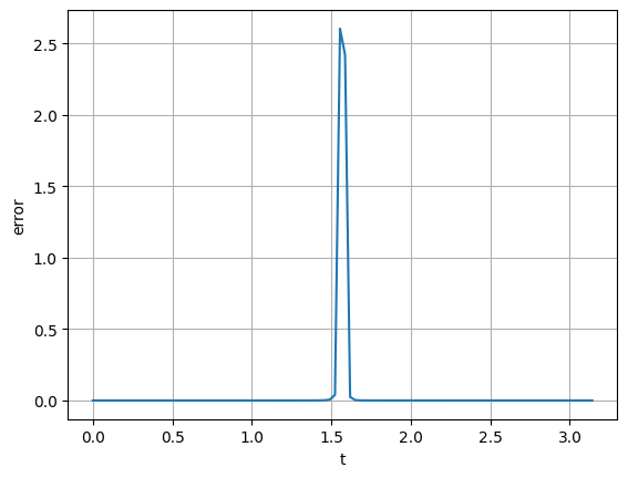
(a) Invariant PINN error.

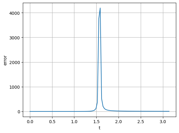
(b) Standard PINN error.

Figure 2: Time series of the squared error for the Schwarz equation (10).

Example 15.

As our second example, we consider the logistic equation

$$u_{t}=u(1-u)$$ (31)

occurring in population growth modeling. Equation (31) admits the one-parameter symmetry group

$$T=t,\qquad U=\frac{u}{1+\epsilon\,ue^{-t}},\qquad\text{where}\qquad\epsilon\in\mathbb{R}.$$

Implementing the algorithm outlined in Section 3.5, we choose the cross-section $\mathcal{K}=\{u=1\}$. This yields the invariantized equation

$$I=\iota(u_{t})=0.$$

The reconstruction equation is

$$\epsilon_{t}=I=0,$$

subject to the initial condition

$$\epsilon(t_{0})=\bigg{(}\frac{1-u_{0}}{u_{0}}\bigg{)}e^{t_{0}},$$

where $u_{0}=0.5$ and our interval of integration is $[0,\pi]$. The solution to the logistic equation is then given by

$$u(t)=\frac{1}{1+\epsilon\,e^{-t}}.$$

As Figure 3 illustrates, the error incurred by the invariant PINN model is significantly smaller, by about a factor of more than 100, than the standard PINN implementation when compared to the exact solution $u(t)=1/(1+e^{-t})$.

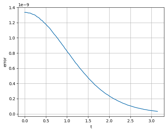
(a) Invariant PINN error.

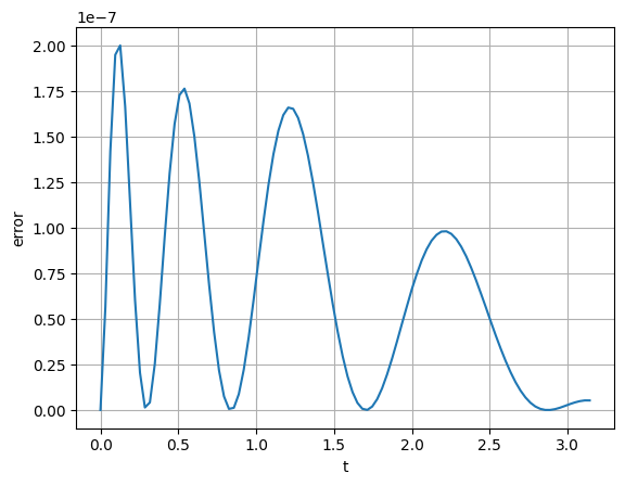
(b) Standard PINN error.

Figure 3: Time series of the squared error for the logistic equation (31).

Example 16.

We now consider the driven harmonic oscillator

$$u_{tt}+u=\sin(t^{a}),$$ (32)

which appears in inductor-capacitor circuits, [33]. In the following we set $a=0.99$, which yields bounded solutions close to resonance occurring when $a=1$. The differential equation (32) admits the two-dimensional symmetry group of transformations

$$T=t,\qquad U=u+\alpha\sin(t)+\beta\cos(t),\qquad\text{where}\qquad\alpha,\beta\in\mathbb{R}.$$

A cross-section to the prolonged action is given by $\mathcal{K}=\{u=u_{t}=0\}$. The invariantization of (32) yields

$$I=\iota(u_{tt})=\sin(t^{a}).$$

The reconstruction equations are

$$\alpha_{t}=\sin(t^{a})\cos(t),\qquad\beta_{t}=-\sin(t^{a})\sin(t),$$ (33)

with initial conditions

$$\alpha(t_{0})=u_{0}\sin(t_{0})+u_{t}^{0}\cos(t_{0}),\qquad\beta(t_{0})=u_{0}\cos(t_{0})-u_{t}^{0}\sin(t_{0}),$$

where, in our numerical simulations, we set $u_{0}=u_{t}^{0}=1$ and integrate over the interval $[0,10]$. Given a solution to the reconstruction equations (33), the solution to the driven harmonic oscillator (32) is

$$u(t)=\alpha(t)\,\sin(t)+\beta(t)\cos(t).$$

Figure 4 shows the error for the invariant PINN implementation and the standard PINN approach compared to the solution obtained using the odeint Runge–Kutta method in scipy.integrate. As in the previous two examples, the invariant version yields substantially better numerical results than the standard PINN method.

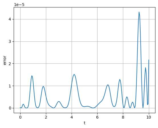
(a) Invariant PINN error

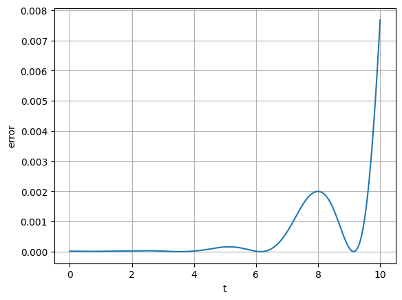
(b) Standard PINN error

Figure 4: Time series of the squared error for the driven harmonic oscillator (32).

Example 17.

We now consider the second order ordinary differential equation

$$u_{tt}=\exp{[-u_{t}]}$$ (34)

with an exponential term. Equation (34) admits a three-dimensional symmetry group action given by

$$T=e^{\epsilon}t+a,\qquad U=e^{\epsilon}u+\epsilon\,e^{\epsilon}x+b,$$

where $a,b,\epsilon\in\mathbb{R}$. In the following, we only consider the one-dimensional group

$$T=e^{\epsilon}t,\qquad U=e^{\epsilon}u+\epsilon\,e^{\epsilon}x.$$

We note that in this example the independent variable is not invariant as in the previous examples. A cross-section to the prolonged action is given by $\mathcal{K}=\{u_{x}=0\}$. Introducing the invariants

$$H=\ln\bigg{[}\frac{1}{1-\iota(t)}\bigg{]}=\ln\bigg{[}\frac{1}{1-tu_{t}}\bigg{]},\qquad I=\iota(u)=\exp[-u_{t}](u-tu_{t}),$$

the invariantization of the differential equation (34) reduces to the first order linear equation

$$I_{H}+I=e^{-H}-1.$$

The reconstruction equation for the left moving frame is simply

$$\epsilon_{H}=1.$$

In terms of $\epsilon$ and $I$, the parametric solution to the original differential equation (34) is

$$t=e^{\epsilon}(1-e^{-H}),\qquad u=e^{\epsilon}(I+\epsilon(1-e^{-H})).$$ (35)

The solution to (34) is known and is given by

$$u(t)=(t+c_{1})\ln(t+c_{1})-t+c_{2},$$ (36)

where $c_{1}$, $c_{2}$ are two integration constants. For the numerical simulations, we use the initial conditions

$$I_{0}=\exp[-u_{t}^{0}](u_{0}-t_{0}u_{t}^{0}),\qquad\epsilon_{0}=u_{t}^{0},$$

where $u_{0}=u(t_{0})$, $u_{t}^{0}=u_{t}(t_{0})$ with $t_{0}=0$, and $c_{1}=\exp(-5)$, $c_{2}=0$ in (36). The interval of integration $[H_{0},H_{f}]$ is given by

$$H_{0}=\ln\bigg{[}\frac{1}{1-t_{0}u_{t}^{0}}\bigg{]},\qquad H_{f}=\ln\bigg{[}\frac{1}{1-t_{f}u_{t}^{f}}\bigg{]},$$ (37)

where $u_{t}^{f}=u_{t}(t_{f})$ and $t_{f}=2$. We choose the interval of integration given by (37), so that when $t$ is given by (35) it lies in the interval $[0,2]$.

Figure 5 shows the error obtained for the invariant PINN model when compared to the exact solution (34), and similarly for the non-invariant PINN model. As in all previous examples, the invariant version drastically outperforms the standard PINN approach.

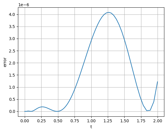
(a) Invariant PINN error.

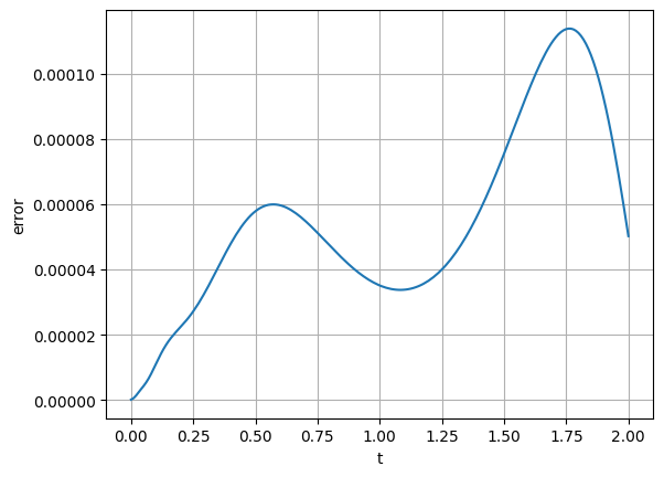
(b) Standard PINN error.

Figure 5: Time series of the squared error for the exponential equation (34).

Example 18.

As our final example, we consider a system of first order ODEs

$$u_{t}=-u+(t+1)v,\qquad v_{t}=u-tv.$$ (38)

This system admits a two-dimensional symmetry group of transformations given by

$$T=t,\qquad U=\alpha u+\beta t,\qquad V=\alpha v+\beta,$$

where $\alpha>0$ and $\beta\in\mathbb{R}$. Working with the cross-section $\mathcal{K}=\{u=1,v=0\}$, the invariantization of (38) yields

$$I=\iota(u_{x})=-1,\qquad J=\iota(v_{x})=1.$$

The reconstruction equations are

$$\alpha_{t}=\alpha(1+t),\qquad\beta_{t}=\alpha$$

subject to the initial conditions $\alpha_{0}=1$, $\beta_{0}=1$, corresponding to the initial conditions $u_{0}=v_{0}=1$, when $t_{0}=0$. In our numerical simulations we integrated over the interval $[0,2]$. The solution to (38) is then given by

$$u(t)=\alpha(t)+t\,\beta(t),\qquad v(t)=\beta(t).$$

As in all previous examples, comparing the numerical solutions to the exact solution

$$u(t)=\sqrt{\frac{2}{\pi}}\,c\,e^{-(t+1)^{2}/2}+c\,t\,\text{erf}\bigg{(}\frac{t+1}{\sqrt{2}}\bigg{)}+kt,\qquad v(t)=c\,\text{erf}\bigg{(}\frac{t+1}{\sqrt{2}}\bigg{)}+k,$$

with $c=\big{(}\sqrt{2/\pi}\,\exp(-1/2)\big{)}^{-1}$ and $k=1-c\,\text{erf}(1/\sqrt{2})$, where $\text{erf}(t)=2/\sqrt{\pi}\int_{0}^{t}e^{-x^{2}}\mathrm{d}x$ is the standard error function, we observe in Figure 6 that the invariant version of the PINN model considerably outperforms its non-invariant counterpart.

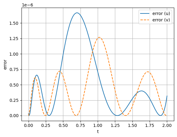
(a) Invariant PINN error.

(b) Standard PINN error.

Figure 6: Time series of the squared error for the system of equations (38).

6 Summary and conclusions

In this paper we have introduced the notion of invariant physics-informed neural networks. These combine physics-informed neural networks with methods from the group analysis of differential equations to simplify the form of the differential equations that have to be solved. In turns, this simplifies the loss function that has to be minimized, and our numerical tests show that the solutions obtained with the invariant model outperformed their non-invariant counterparts, and typically considerably so. Table 1 summarizes the examples considered in the paper and shows that the invariant PINN outperforms vanilla PINN for the examples considered.

Example	Invariant PINN	Vanilla PINN
Schwarz (10)	$5.1\cdot 10^{-2}\pm 4.1\cdot 10^{-2}$	$96.89\pm 0.81$
Logistic (31)	$2.6\cdot 10^{-10}\pm 1.8\cdot 10^{-10}$	$3\cdot 10^{-2}\pm 4.6\cdot 10^{-5}$
Harmonic (32)	$5.8\cdot 10^{-6}\pm 4.8\cdot 10^{-6}$	$1.4\cdot 10^{-5}\pm 2.3\cdot 10^{-5}$
Exponential (34)	$3.2\cdot 10^{-7}\pm 2.2\cdot 10^{-7}$	$2.6\cdot 10^{-5}\pm 3.6\cdot 10^{-5}$
System (38)	$9.4\cdot 10^{-7}\pm 2.0\cdot 10^{-7}$	$6.6\cdot 10^{-6}\pm 7.9\cdot 10^{-6}$

Table 1: Mean square error with standard deviation averaged over five runs for all examples considered in Section 5.

The proposed method is fully algorithmic and as such can be applied to any system of differential equations that is strongly invariant under the prolonged action of a group of Lie point symmetries. It is worth noting that the work proposed here parallels some of the work on invariant discretization schemes which, for ordinary differential equations, also routinely outperform their non-invariant counterparts. We have observed this to also be the case for physics-informed neural networks.

Lastly, while we have restricted ourselves here to the case of ordinary differential equations, our method extends to partial differential equations as well. Though, when considering partial differential equations, it is not sufficient to project the equations onto the space of differential invariants as done in this paper. As explained in [36], integrability conditions among the differential invariants must also be added to the invariantized differential equations. In the multivariate case, the reconstruction equations (23) will then form a system of first order partial derivatives for the left moving frame. Apart from these modifications, invariant physics-informed neural networks can also be constructed for partial differential equations, which will be investigated elsewhere.

References

- [1] A. G. Baydin, B. A. Pearlmutter, A. A. Radul, and J. M. Siskind. Automatic differentiation in machine learning: a survey. J. Mach. Learn. Res., 18:Paper No. 153, 2018.
- [2] A. Bihlo. Invariant meshless discretization schemes. J. Phys. A: Math. Theor., 46(6):062001 (12 pp), 2013.
- [3] A. Bihlo. Improving physics-informed neural networks with meta-learned optimization. arXiv preprint arXiv:2303.07127, 2023.
- [4] A. Bihlo, J. Jackaman, and F. Valiquette. Invariant variational schemes for ordinary differential equations. Stud. Appl. Math., 148(3):991–1020, 2022.
- [5] A. Bihlo and J.-C. Nave. Convecting reference frames and invariant numerical models. J. Comput. Phys., 272:656–663, 2014.
- [6] A. Bihlo and R. O. Popovych. Physics-informed neural networks for the shallow-water equations on the sphere. J. of Comput. Phys., 456:111024, 2022.
- [7] A. Bihlo and F. Valiquette. Symmetry-preserving numerical schemes. In Symmetries and Integrability of Difference Equations, pages 261–324. Springer, 2017.
- [8] A. Bihlo and F. Valiquette. Symmetry-preserving finite element schemes: An introductory investigation. SIAM J. Sci. Comput., 41(5):A3300–A3325, 2019.
- [9] G. W. Bluman, A. F. Cheviakov, and S. C. Anco. Application of symmetry methods to partial differential equations, volume 168 of Applied Mathematical Sciences. Springer, New York, 2010.
- [10] G.W. Bluman and S. Kumei. Symmetries and differential equations. Springer, New York, 1989.
- [11] R. Brecht, D. R. Popovych, A. Bihlo, and R. O. Popovych. Improving physics-informed deeponets with hard constraints. arXiv preprint arXiv:2309.07899, 2023.
- [12] C. Budd and V. A. Dorodnitsyn. Symmetry-adapted moving mesh schemes for the nonlinear Schrödinger equation. J. Phys. A, 34(48):10387–10400, 2001.
- [13] T. Cohen and M. Welling. Group equivariant convolutional networks. In International conference on machine learning, pages 2990–2999. PMLR, 2016.
- [14] V. A. Dorodnitsyn. Transformation groups in mesh spaces. J. Sov. Math., 55(1):1490–1517, 1991.
- [15] M. Fels and P. J. Olver. Moving coframes. II. Regularization and theoretical foundations. Acta Appl. Math., 55:127–208, 1999.
- [16] M. Finzi, M. Welling, and A. G. Wilson. A practical method for constructing equivariant multilayer perceptrons for arbitrary matrix groups. In ICML, pages 3318–3328. PMLR, 2021.
- [17] P. E. Hydon. Symmetry methods for differential equations. Cambridge University Press, Cambridge, 2000.
- [18] A. D. Jagtap, E. Kharazmi, and G. E. Karniadakis. Conservative physics-informed neural networks on discrete domains for conservation laws: applications to forward and inverse problems. Comput. Methods Appl. Mech. Eng., 365:113028, 2020.
- [19] P. Kim. Invariantization of numerical schemes using moving frames. BIT Numerical Mathematics, 47(3):525–546, 2007.
- [20] D. P. Kingma and J. Ba. Adam: A method for stochastic optimization. arXiv:1412.6980, 2014.
- [21] I. A. Kogan and P. J. Olver. Invariant Euler–Lagrange equations and the invariant variational bicomplex. Acta Appl. Math., 76(2):137–193, 2003.
- [22] A. Krishnapriyan, A. Gholami, S. Zhe, R. Kirby, and M. W. Mahoney. Characterizing possible failure modes in physics-informed neural networks. Advances in Neural Information Processing Systems, 34:26548–26560, 2021.
- [23] I. E. Lagaris, A. Likas, and D. I. Fotiadis. Artificial neural networks for solving ordinary and partial differential equations. IEEE Trans. Neural Netw., 9(5):987–1000, 1998.
- [24] L. Lu, P. Jin, G. Pang, Z. Zhang, and G. E. Karniadakis. Learning nonlinear operators via DeepONet based on the universal approximation theorem of operators. Nat. Mach. Intell., 3(3):218–229, 2021.
- [25] E. L. Mansfield. A practical guide to the invariant calculus, volume 26. Cambridge University Press, 2010.
- [26] L. McClenny and U. Braga-Neto. Self-adaptive physics-informed neural networks using a soft attention mechanism. arXiv preprint arXiv:2009.04544, 2020.
- [27] P. J. Olver. Application of Lie groups to differential equations. Springer, New York, 2000.
- [28] P. J. Olver. Geometric foundations of numerical algorithms and symmetry. Appl. Algebra Engrg. Comm. Comput., 11(5):417–436, 2001.
- [29] P. J. Olver. Equivalence, invariants and symmetry. Cambridge University Press, Cambridge, 2009.
- [30] M. Raissi, P. Perdikaris, and G. E. Karniadakis. Physics-informed neural networks: A deep learning framework for solving forward and inverse problems involving nonlinear partial differential equations. J. Comput. Phys., 378:686–707, 2019.
- [31] R. Rebelo and F. Valiquette. Symmetry preserving numerical schemes for partial differential equations and their numerical tests. J. of Diff. Eq. and Appl., 19(5):738–757, 2013.
- [32] R. Rebelo and F. Valiquette. Invariant discretization of partial differential equations admitting infinite-dimensional symmetry groups. J. Difference Equ. Appl., 21(4):285–318, 2015.
- [33] R.A. Serway and J.W. Jewett. Physics for Scientists and Engineers. Brooks/Cole, 2003.
- [34] Y.I. Shokin. The method of differential approximation. Springer, 1983.
- [35] Z. Tang, Z. Fu, and S. Reutskiy. An extrinsic approach based on physics-informed neural networks for pdes on surfaces. Mathematics, 10(16):2861, 2022.
- [36] R. Thompson and F. Valiquette. Group foliation of differential equations using moving frames. Forum of Math.: Sigma, 3:e22, 2015.
- [37] M. Vaquero, J. Cortés, and D.M. de Diego. Symmetry preservation in hamiltonian systems: Simulation and learning.
- [38] S. Wang, S. Sankaran, and P. Perdikaris. Respecting causality is all you need for training physics-informed neural networks. arXiv preprint arXiv:2203.07404, 2022.
- [39] N. N. Yanenko and Y. I. Shokin. The group classification of difference schemes for the system of equations of gas dynamics. Tr. Mat. Inst. Akad. Nauk SSSR, 122:85–97, 1973.