Fundamental MHD scales – II: the kinematic phase of the supersonic small-scale dynamo

Abstract

The small-scale dynamo (SSD) amplifies weak magnetic fields exponentially fast via kinetic motions. While there exist well-established theories for SSDs in incompressible flows, many astrophysical environments SSDs operate in supersonic, turbulent gas. To understand the impact of compressibility on SSD-amplified magnetic fields, we perform an extensive set of visco-resistive SSD simulations, covering a wide range of sonic Mach number $\mathcal{M}$, hydrodynamic Reynolds number $\mathrm{Re}$, and magnetic Prandtl number $\mathrm{Pm}$. We develop simple, robust methods for measuring characteristic kinetic and magnetic energy dissipation scales $\ell_{\nu}$ and $\ell_{\eta}$, as well as the scale at which magnetic fields are strongest $\ell_{\mathrm{p}}$ during the kinematic phase of these simulations. We show that $\ell_{\nu}/\ell_{\eta}\sim\mathrm{Pm}^{1/2}$ is a universal feature in the kinematic phase of $\mathrm{Pm}\geq 1$ SSDs, regardless of $\mathcal{M}$ or $\mathrm{Re}$, and we confirm earlier predictions that SSDs operating in incompressible plasmas (either $\mathcal{M}\leq 1$ or $\mathrm{Re}<\mathrm{Re}_{\mathrm{crit}}\approx 100$) concentrate magnetic energy at the smallest scales allowed by magnetic dissipation, $\ell_{\mathrm{p}}\sim\ell_{\eta}$, and produce fields organised with field strength and field-line curvature inversely correlated. However, we show that these predictions fail for compressible SSDs ($\mathcal{M}>1$ and $\mathrm{Re}>\mathrm{Re}_{\mathrm{crit}}$), where shocks concentrate magnetic energy in large-scale, over-dense, coherent structures in the plasma, with characteristic size $\ell_{\mathrm{p}}\sim(\ell_{\mathrm{turb}}/\ell_{\mathrm{shock}})^{1/3}\ell_{\eta}\gg\ell_{\eta}$, where $\ell_{\mathrm{shock}}\sim\mathcal{M}^{2}/[\mathrm{Re}\,(\mathcal{M}-1)^{2}]$ is the characteristic shock width, and $\ell_{\mathrm{turb}}$ is the outer scale of the turbulent field. Moreover, in this compressible regime, magnetic field-line curvature becomes almost independent of the field strength. We discuss the implications of these results for galaxy mergers and for cosmic-ray transport models in the interstellar medium that are sensitive to field-line curvature statistics.

1 Introduction

As far as we understand, the Universe was born without magnetic fields. This, however, stands in stark contrast with the present-day Universe, where dynamically important magnetic fields are observed to be ubiquitous (see Krumholz & Federrath, 2019; Brandenburg & Ntormousi, 2023, for recent reviews on magnetic fields in galaxies and their impact on star formation). The origin of these fields remains uncertain, but two main candidates exist: phase transitions during inflation, which could have generated fields with strengths ranging from $10^{-36}$ to $10^{-8}\,\mathrm{G}$, varying on $\sim\mbox{Mpc}$ scales (Quashnock et al., 1989; Sigl et al., 1997; Kahniashvili et al., 2013), and battery processes during the epoch of re-ionisation ($z\sim 35$–$6$) (Biermann, 1950; Naoz & Narayan, 2013), which could have produced fields of around $10^{-24}\,\mathrm{G}$ on $\sim 10\,\mbox{kpc}$ scales. Regardless of which mechanism seeded the first magnetic fields, primordial fields are believed to have decayed until the structure formation era at $z\sim 2$ (e.g.,  Brandenburg et al., 2017; Vachaspati, 2021; Hosking & Schekochihin, 2022; Mtchedlidze et al., 2022, 2023), by which time they would have been more than $15$ orders of magnitude weaker than the $\sim\mu\mathrm{G}$ fields observed on $\sim\mbox{kpc}$ scales in the Milky Way and in other nearby galaxies (e.g.,  Kulsrud et al., 1997; Beck et al., 2019; Shah & Seta, 2021; Lopez-Rodriguez et al., 2022). Present-day magnetic fields, therefore, cannot simply be relics from electroweak phase transitions or battery processes in the early Universe, and instead some mechanism must have amplified them dramatically.

Dynamo action is believed to be the most plausible mechanism for amplifying primordially-produced fields to the levels we observe in the present day (e.g.,  Latif et al., 2013; Mtchedlidze et al., 2022, 2023), and broadly describes the process by which initially weak magnetic fields are amplified and subsequently maintained through the conversion of kinetic into magnetic energy (see Rincon 2019; Brandenburg & Ntormousi 2023 for recent reviews, and Tzeferacos et al. 2018; Bott et al. 2021, 2022 for recent laboratory experiments). Such processes are categorised either as small-scale dynamos (SSDs) or large-scale dynamos (LSDs), determined by the scale on which magnetic fields are grown relative to the kinetic fields that amplify them. In the current paradigm for the origin of galactic magnetic fields, both SSDs and LSDs are believed to be important, but are understood to play very different roles (see Bhat et al., 2016; Pakmor et al., 2017; Rieder & Teyssier, 2017a, b; Steinwandel et al., 2023; Gent et al., 2023, for recent works).

Starting with initially weak seed fields, SSDs that operate in regimes relevant for the interstellar medium (ISM) of galaxies, for example, follow a three-stage process: (1) first, random kinetic motions (e.g.,  Vainshtein et al., 1972; Zel’Dovich et al., 1984; Archontis et al., 2003) amplify magnetic energy exponentially fast-in-time (also termed the kinematic phase of the SSD), then, (2) once magnetic fields are strong enough to impart a backreation on the flow, via the Lorentz force, the growth rate slows down to a linear-in-time growth (e.g.,  Schekochihin et al., 2004; Xu & Lazarian, 2016; Seta & Federrath, 2020), and (3) finally, once the magnetic field is in close equipartition with kinetic energy, the field strength saturates and continues to be maintained at this level via the kinetic field (e.g.,  Schekochihin et al., 2002b; Seta & Federrath, 2021; Beattie et al., 2023). Galactic LSDs are also capable of exponential magnetic growth, which could be driven by a mix of helical turbulence (e.g.,  Bhat et al., 2016; Rincon, 2021), galactic differential rotation/shear (e.g.,  Käpylä et al., 2008; Squire & Bhattacharjee, 2015), and magnetic instabilities (e.g.,  Johansen & Levin, 2008; Qazi et al., 2023). However, due to catastrophic quenching at low magnetic resistivity, they are not believed to be capable of amplifying primordial fields to the magnitudes we observe today (see Brandenburg & Ntormousi, 2023, for a recent, thorough review of LSDs).

SSDs supported by supernova-driven turbulence are capable of amplifying magnetic energy far more rapidly than LSDs (Schober et al., 2012; Gent et al., 2023), and have been shown (using simulations) to be capable of amplifying primordial magnetic fields with an e-folding time of $\approx 100\,\mbox{Myr}$, reaching a saturated field strength of $10$–$50\,\mu\mathrm{G}$ (corresponding to $\approx 10\%$ of equipartition with the kinetic energy) by $z\sim 3$–$2$ (Pakmor et al., 2017; Rieder & Teyssier, 2016, 2017a; Steinwandel et al., 2023), thus making the kinematic stage of the SSD an important phase to study. By contrast, LSDs are too slow to produce saturated fields at such high redshifts, but are efficient at reorganising fields to produce large scale, coherent structures. Thus, as galaxies become more quiescent, rotation creates a LSD that operates on the SSD-generated fields to produce the larger scale, ordered fields that we see today (Rieder & Teyssier, 2017a; Gent et al., 2023).

This picture has been challenged, however, by the detection of $\lesssim 500\,\mu\mathrm{G}$ magnetic fields ordered on $5\,\mbox{kpc}$ scales in a distant ($z\sim 2.6$) gravitationally micro-lensed galaxy (Geach et al., 2023). While the field strength remains poorly constrained, the fact that it is ordered on $\sim\mbox{kpc}$ scales poses a problem for the model outlined above, since a LSD would not have had enough time to become established at $z\sim 2.6$, and SSDs have been traditionally thought to produce fields that are chaotic on large scales, and only become ordered on the smallest scales allowed by magnetic dissipation (e.g.,  Schekochihin et al., 2004; Kriel et al., 2022; Brandenburg et al., 2023), which are expected to be $\ll\mbox{pc}$ in size for ISM conditions (Marchand et al., 2016). A similar problem exists in galaxy mergers, where the rapid growth in magnetic field strengths seen in simulations point to SSD action, but the fields produced are correlated on $\sim\mbox{kpc}$ scales, which have been thought to be too large scale for a SSD to generate (e.g.,  Rodenbeck & Schleicher, 2016; Basu et al., 2017; Brzycki & ZuHone, 2019; Whittingham et al., 2021).

In this paper we explore a possible resolution to the problems highlighted above for galaxy mergers. The expectation that SSDs only produce small-scale structure is based on extensive explorations of SSDs in incompressible (e.g., subsonic) flow regimes, which is the regime we explored in Paper I of this series (Kriel et al., 2022, herein Fundamental Scales I). In Fundamental Scales I, we used direct numerical simulations to confirm theoretically predicted properties of magnetic fields produced during the kinematic phase (see seminal works by, e.g.,  Kazantsev, 1968; Vainshtein, 1982; Vincenzi, 2002; Schekochihin et al., 2004; Boldyrev & Cattaneo, 2004), highlighting how the bulk of magnetic energy is localised at the smallest possible scales in the incompressible problem, i.e., the scale where magnetic fields dissipate. However, both the first galaxies (Maio et al., 2011; Mandelker et al., 2020) and later galaxy mergers (Geng et al., 2012; Sparre et al., 2022) are expected to host highly compressible (i.e., supersonic) turbulence, since the great majority of their mass and a substantial fraction of their volume consists of dense, atomic and molecular gas (Cox et al., 2006; Krumholz et al., 2009; Popping et al., 2014; Nandakumar & Dutta, 2023) where rapid cooling keeps the sound speed well below the characteristic flow velocity (Rees & Ostriker, 1977; White & Rees, 1978; Birnboim & Dekel, 2003; Krumholz et al., 2020; Li et al., 2020). While it has been shown that supersonic flows decreases the efficiency of SSDs (Federrath et al., 2011, 2014; Achikanath Chirakkara et al., 2021; Seta & Federrath, 2021, 2022; Hew & Federrath, 2023), there has to date, been no systematic study of how compressibility changes magnetic field geometry, characteristic scales, or structure. Our goal in this paper is to provide such a study, and in turn to explore its implications both for galaxy mergers and for other phenomena that depend on magnetic field structure, most notably cosmic ray transport (e.g.,  Kempski et al., 2023; Lemoine, 2023).

The remainder of this paper is structured as follows. In Section 2 we describe the numerical simulation suite we use to develop our theoretical model for compressible SSDs. In Section 3 we present and interpret the simulation results, and in Section 4 we discuss their implications for a variety of astrophysical systems. We summarise our results and conclusions in Section 5.

2 Numerical Approach

In this study we use direct numerical simulations to explore the kinematic phase of SSDs in flows ranging from viscous to turbulent, and subsonic to supersonic. In Section 2.1 we introduce the basic equations that we solve, the numerical method by which we do so, and the initial conditions for our simulations. In Section 2.2 we introduce the key dimensionless parameters that describe different flow regimes, and how we vary these parameters to explore different flow properties. In Section 2.3, we then discuss issues of convergence.

2.1 Numerical Model, Method, and Initial Conditions

For all the simulations in this study, we solve the compressible set of non-ideal (visco-resistive) magnetohydrodynamical (MHD) fluid equations, which in conservative form are

$$\frac{\partial\rho}{\partial t}+\nabla\cdot(\rho\mathrm{{\mn@boldsymbol{\mathit{u}}}}) =0,$$ (1)

$$\frac{\partial\rho\mathrm{{\mn@boldsymbol{\mathit{u}}}}}{\partial t}+\nabla\cdot\bigg{[}\rho\mathrm{{\mn@boldsymbol{\mathit{u}}}}\otimes\mathrm{{\mn@boldsymbol{\mathit{u}}}}-\frac{1}{4\pi}\mathrm{{\mn@boldsymbol{\mathit{b}}}}\otimes\mathrm{{\mn@boldsymbol{\mathit{b}}}}\hskip 70.0001pt\ignorespaces$$

$$+\left(c_{\mathrm{s}}^{2}\rho+\frac{b^{2}}{8\pi}\right)\textbf{{I}}-2\nu\rho\textbf{{S}}\bigg{]} =\rho\mathrm{{\mn@boldsymbol{\mathit{f}}}},$$ (2)

$$\frac{\partial\mathrm{{\mn@boldsymbol{\mathit{b}}}}}{\partial t}-\nabla\times\left(\mathrm{{\mn@boldsymbol{\mathit{u}}}}\times\mathrm{{\mn@boldsymbol{\mathit{b}}}}-\eta\mathrm{{\mn@boldsymbol{\mathit{j}}}}\right) =0,$$ (3)

$$\nabla\cdot\mathrm{{\mn@boldsymbol{\mathit{b}}}} =0,$$ (4)

for an isothermal plasma evolving over a uniformly discretised, cubic-domain $\ell_{(x,y,z)}\in[0,\ell_{\mathrm{box}}]$, with triply periodic boundary conditions. Here we use constant (in both space and time) kinematic shear viscosity and Ohmic resistivity, parameterised by the coefficients $\nu$ and $\eta$, respectively, in combination with an external forcing field $\mathrm{{\mn@boldsymbol{\mathit{f}}}}$, to achieve flows with desired plasma numbers (see Section 2.2 for details). The remaining quantities in the equations are the gas density $\rho$, the gas velocity $\mathrm{{\mn@boldsymbol{\mathit{u}}}}$, the sound speed $c_{\mathrm{s}}$, the current density $\mathrm{{\mn@boldsymbol{\mathit{j}}}}=\nabla\times\mathrm{{\mn@boldsymbol{\mathit{b}}}}/(4\pi)$, and the magnetic field $\mathrm{{\mn@boldsymbol{\mathit{b}}}}=\mathrm{{\mn@boldsymbol{\mathit{b}}}}_{0}+\mathrm{{\mn@boldsymbol{\mathit{\delta b}}}}$, which has mean field $\mathrm{{\mn@boldsymbol{\mathit{b}}}}_{0}$, and fluctuating (turbulent) field $\mathrm{{\mn@boldsymbol{\mathit{\delta b}}}}$ components. Finally, our viscosity model is based on the traceless strain rate tensor, S, where

$$\textbf{{S}}=\frac{1}{2}\left(\nabla\otimes\mathrm{{\mn@boldsymbol{\mathit{u}}}}+\left(\nabla\otimes\mathrm{{\mn@boldsymbol{\mathit{u}}}}\right)^{T}\right)-\frac{1}{3}\left(\nabla\cdot\mathrm{{\mn@boldsymbol{\mathit{u}}}}\right)\textbf{{I}},$$ (5)

and $\otimes$ is the tensor product $\nabla\otimes\mathrm{{\mn@boldsymbol{\mathit{u}}}}\equiv\partial_{i}u_{j}$.

We solve Equation 1-Equation 4 with a modified version of the finite-volume flash code (Fryxell et al., 2000; Dubey et al., 2008), employing a second-order conservative MUSCL-Hancock 5-wave approximate Riemann solver, described in Bouchut et al. (2007, 2010), and implemented into flash by Waagan et al. (2011), who showed that it possesses excellent stability properties for highly supersonic MHD flows, with improved efficiency and stability compared with Roe-type solvers. Since our primary interest lies in studying the effects of shocks (a hallmark of supersonic flows), this solver proves highly suitable. Moreover, we utilise the parabolic divergence-cleaning method described by Marder (1987) to enforce that $\nabla\cdot\mathrm{{\mn@boldsymbol{\mathit{b}}}}=0$ errors are diffused away.

All our simulations use a dimensionless unit system where the simulation box size $\ell_{\mathrm{box}}=1$, mean density $\rho_{0}=1$, the sound speed $c_{\mathrm{s}}=1$, and magnetic fields are measured in units of $\rho_{0}^{1/2}c_{\mathrm{s}}=1$. We initialise every simulation with uniform density $\rho=\rho_{0}=1$, zero velocity $\mathrm{{\mn@boldsymbol{\mathit{u}}}}=\mathrm{{\mn@boldsymbol{\mathit{0}}}}$, and zero mean magnetic field $\mathrm{{\mn@boldsymbol{\mathit{b}}}}_{0}=\mathrm{{\mn@boldsymbol{\mathit{0}}}}$. Since there is no mean magnetic field, and magnetic flux through the simulation volume is conserved, only a fluctuating component can exist, $\mathrm{{\mn@boldsymbol{\mathit{b}}}}=\mathrm{{\mn@boldsymbol{\mathit{\delta b}}}}$. We initialise this fluctuating component with a spectral distribution (using TurbGen; Federrath et al., 2022) that is non-zero only over the wavenumber range $1\leq k\ell_{\mathrm{box}}/2\pi\leq 3$, with a parabolic profile that peaks at $k\ell_{\mathrm{box}}/2\pi=2$, and goes to zero at $k\ell_{\mathrm{box}}/2\pi=1$ and $k\ell_{\mathrm{box}}/2\pi=3$. Here, the isotropic wavenumber $k$ is defined as per usual: $k\equiv 2\pi/\ell$. We choose the amplitude of this initial parabolic $\mathrm{{\mn@boldsymbol{\mathit{\delta b}}}}$ profile such that the plasma–$\beta\equiv p_{\rm th}/p_{\mathrm{mag}}=8\pi c_{\mathrm{s}}^{2}\rho_{0}/b^{2}=10^{10}$. We note that the exact configuration of the initial seed $\mathrm{{\mn@boldsymbol{\mathit{\delta b}}}}$ field is not important, because it is quickly forgotten by the Markovian-like flow dynamics, and has been shown to not affect the amplification nor the final saturation of the dynamo (Seta & Federrath, 2020; Bott et al., 2022; Beattie et al., 2023).

2.2 Dimensionless Numbers and Flow Regimes

In this study we explore 34 different simulation configurations, each parameterised by a set of dimensionless numbers that characterise the MHD flow regime. Here we introduce each of these numbers, as well as the range of values over which we vary them, before summarising our full set of simulations in Table 1.

2.2.1 Sonic Mach Number

For all our simulations we produce an isotropic, smoothly varying (in time and space) acceleration field via the forcing term, $\mathrm{{\mn@boldsymbol{\mathit{f}}}}$, in Equation 2, which is modelled with a generalisation of the Ornstein-Uhlenbeck process in wavenumber-space (Eswaran & Pope, 1988; Schmidt et al., 2006; Schmidt et al., 2009; Federrath et al., 2010, 2022) using TurbGen. We choose to drive the acceleration field with purely solenoidal modes, i.e., $\nabla\cdot\mathrm{{\mn@boldsymbol{\mathit{f}}}}=0$, because they produce motions that are the most efficient at amplifying magnetic energy (Federrath et al., 2011, 2014; Martins Afonso et al., 2019; Chirakkara et al., 2021), and tune the amplitude of $\mathrm{{\mn@boldsymbol{\mathit{f}}}}$ in each of our simulations to achieve a root-mean-squared (rms) gas velocity dispersion, $\left\langle u\right\rangle_{\mathcal{V}}^{1/2}$, on the driving (outer) scale, $\ell_{\mathrm{turb}}$, that lies within $5\%$ of our desired value, $u_{\mathrm{turb}}$; the notation $\left\langle q\right\rangle_{\mathcal{V}}$ indicates the volume average of quantity $q$ over the entire simulation domain $\mathcal{V}\equiv\ell_{\mathrm{box}}^{3}$. We choose $\ell_{\mathrm{turb}}=\ell_{\mathrm{box}}/2$ for all of our simulations to maximise the scale separation between kinetic fields and the small-scale magnetic fields they generate, which we achieve by driving $\mathrm{{\mn@boldsymbol{\mathit{f}}}}$ with a parabolic power spectrum that is non-zero only over the wavenumber range $1\leq k\ell_{\mathrm{box}}/2\pi\leq 3$, peaking at $k\ell_{\mathrm{box}}/2\pi=2$, and falling to zero at $k\ell_{\mathrm{box}}/2\pi=1$ and $k\ell_{\mathrm{box}}/2\pi=3$. The corresponding autocorrelation time of $\mathrm{{\mn@boldsymbol{\mathit{f}}}}$, and hence the kinetic field, is

$$t_{\mathrm{turb}}=2\pi/(k_{\mathrm{turb}}u_{\mathrm{turb}}).$$ (6)

Even though $c_{\mathrm{s}}=1$ in our simulations, it is convenient to express the flow velocity relative to the sound speed, i.e., the sonic Mach number

$$\mathcal{M} \equiv\frac{u_{\mathrm{turb}}}{c_{\mathrm{s}}}.$$ (7)

To study the effect of compressibility, we run simulations spanning a wide range of $\mathcal{M}$, with $\mathcal{M}=0.3,1,5$, and $10$. On the lower end of $\mathcal{M}$, we run 11 simulations with $\mathcal{M}=0.3$, where incompressibility in the probability density function (PDF) of $\mathcal{M}$ values in $\mathcal{V}$ holds up to $3$-sigma fluctuations (assuming Gaussianity). This is the regime we explored in Fundamental Scales I, and is relevant for studying Kolmogorov (1941)-like turbulence. We also run a set of four transsonic simulations, $\mathcal{M}=1$, but then turn most of our attention towards the supersonic flow regime, where we run 16 simulations with $\mathcal{M}=5$ and three simulations with $\mathcal{M}=10$. Here, in the highly-compressible ($\mathcal{M}\gtrsim 1$) flow regime, one expects to see Burgers (1948)-like turbulence (see for example Federrath, 2013; Federrath et al., 2021).

2.2.2 Hydrodynamic Reynolds Number

The second dimensionless parameter that characterises our simulations is the hydrodynamic Reynolds number

Re $$\equiv\frac{|\nabla\cdot(\rho\mathrm{{\mn@boldsymbol{\mathit{u}}}}\otimes\mathrm{{\mn@boldsymbol{\mathit{u}}}})|}{|\nabla\cdot(2\nu\rho\textbf{{S}})|}\sim\frac{u_{\mathrm{turb}}\,\ell_{\mathrm{turb}}}{\nu},$$ (8)

which describes the relative importance of inertial to viscous forces in a flow. In Fundamental Scales I we found evidence that $\mbox{Re}\approx\mbox{Re}_{\mathrm{crit}}\approx 100$ is a critical value for Re during the kinematic phase, separating viscous ($\mbox{Re}<\mbox{Re}_{\mathrm{crit}}$) from turbulent ($\mbox{Re}>\mbox{Re}_{\mathrm{crit}}$) flows, with several flow properties changing across this boundary. For example, velocity gradients – which are responsible for viscous dissipative events (see for example Schumacher et al., 2014) – have sub-Gaussian kurtosis in flows with $\mbox{Re}<\mbox{Re}_{\mathrm{crit}}$, and super-Gaussian kurtosis (i.e., intermittent velocity fluctuations) in $\mbox{Re}>\mbox{Re}_{\mathrm{crit}}$ flows. Similarly, the kinetic energy dissipation (viscous) scale follows the theoretically-expected scaling $\ell_{\nu}\sim\mbox{Re}^{3/4}$ (Kolmogorov, 1941) when $\mbox{Re}>\mbox{Re}_{\mathrm{crit}}$, and then as $\ell_{\nu}\sim\mbox{Re}^{3/8}$ when $\mbox{Re}<\mbox{Re}_{\mathrm{crit}}$ (Fundamental Scales I). While $\ell_{\nu}$ is the characteristic viscous scale, there are in fact a whole range of scales $\lesssim\ell_{\nu}$ over which dissipation takes place (e.g.,  Frisch & Vergassola, 1991; Chen et al., 1993), which have also been shown to be directly affected by the degree of intermittency of velocity gradient fluctuations (e.g.,  Schumacher, 2007).

Based on this, we explore $10\leq\mbox{Re}\leq 3000$, where we run most of our simulations with $\mbox{Re}>100$ (in the turbulent regime), and dedicate a small portion of our simulations to $10\leq\mbox{Re}\leq 100$, to explore the transitional regime towards viscous flows.

2.2.3 Magnetic Prandtl Number

Our final two dimensionless numbers are the magnetic Reynolds number,

Rm $$\equiv\frac{|\nabla\times(\mathrm{{\mn@boldsymbol{\mathit{u}}}}\times\mathrm{{\mn@boldsymbol{\mathit{b}}}})|}{|\eta\nabla\times\mathrm{{\mn@boldsymbol{\mathit{j}}}}|}\sim\frac{u_{\mathrm{turb}}\,\ell_{\mathrm{turb}}}{\eta},$$ (9)

which, analogously to the hydrodynamic Reynolds number, characterises the relative importance of magnetic induction compared with magnetic (Ohmic) dissipation, and the magnetic Prandtl number,

$$\mbox{Pm}\equiv\frac{\mbox{Rm}}{\mbox{Re}}\sim\frac{\nu}{\eta}.$$ (10)

Pm characterises the relative strength of the magnetic and kinetic energy dissipation, and thereby gives us control of the relative position of the characteristic kinetic and magnetic energy dissipation scales, $\ell_{\nu}$ and $\ell_{\eta}$, respectively. We focus on the $\mbox{Pm}\geq 1$ regime, because it is relevant for most of the gas in the ISM, and explore $1\leq\mbox{Pm}\leq 300$.

Now, during the kinematic phase of $\mathcal{M}<1$, $\mbox{Pm}>1$ SSDs, there exist well-established theoretical expectations for the relationship between key MHD length scales: $\ell_{\mathrm{turb}}$, $\ell_{\nu}$, and $\ell_{\eta}$, along with the scale $\ell_{\mathrm{p}}$ on which magnetic fields are strongest. In this regime, Schekochihin et al. (2002b, 2004) predicted, and Fundamental Scales I, and Brandenburg et al. (2023) confirmed numerically, that $\ell_{\mathrm{p}}\sim\ell_{\eta}\sim\ell_{\nu}\,\mbox{Pm}^{-1/2}$ (i.e., magnetic energy is strongest on the magnetic dissipation scale). One of the primary goals of our study is to test whether this hierarchy of scales also holds in the $\mathcal{M}>1$ regime.

2.2.4 Choice of Simulation Parameters

The discussion of dimensionless numbers above motivates our choice of simulation parameters. To determine the scaling behaviour of $\ell_{\eta}$ and $\ell_{\mathrm{p}}$ in compressible flows, we first run a set of eight simulations with $\mbox{Rm}=3000$, where we vary $1\leq\mbox{Pm}\leq 300$ while keeping $\mathcal{M}=5$. To isolate the role of compressibility, we then also run a subset of these simulations with $\mathcal{M}=0.3,1$, and $10$. Next, we run three $\mbox{Re}=500$, $\mathcal{M}=5$ simulations, with $\mbox{Pm}=1,2$, and $4$, and four $\mbox{Re}=10$, $\mathcal{M}=5$ simulations with $25\leq\mbox{Pm}\leq 250$. Then, to explore the transition from turbulent to viscous flows, we run a set of four $\mathcal{M}=0.3$ simulations, where we fix $\mbox{Rm}=500$ and vary $1\leq\mbox{Pm}\leq 50$. Finally, we run two simulations with $\mbox{Re}=2000$ and $\mbox{Pm}=5$ (which gives $\mbox{Rm}=10000$), with $\mathcal{M}=0.3$ and $5$, respectively, to confirm that our findings in both the subsonic and supersonic regimes hold in the high-Rm limit.

We summarise the full set of simulations we carry out in Table 1. In this table, and throughout the remainder of this paper, we adopt a naming convention whereby simulations are named $\mathcal{M}$MMMReRRRPmPPP, where MMM, RRR, and PPP give the numerical values of the sonic Mach number, hydrodynamic Reynolds number, and magnetic Prandtl number for that simulation, respectively. Thus, for example $\mathcal{M}$0.3Re600Pm5 indicates a simulation with $\mathcal{M}=0.3$, $\mbox{Re}=600$, and $\mbox{Pm}=5$.

2.3 Numerical Convergence in Time and Resolution

To ensure well-sampled statistics, we run all of our simulations for a duration of $t=100\,t_{\mathrm{turb}}$ (i.e., 100 autocorrelation times of the forcing field), which we show below extends well beyond the kinematic phase and into the saturated state of the dynamo for all of our simulations. We also collect data every $t=0.1\,t_{\mathrm{turb}}$ to ensure well-sampled temporal statistics.

To ensure convergence with regard to spatial resolution, we systematically run each of our simulation setups at progressively higher resolution, until our measurements of key characteristic scales: $\ell_{\nu}$, $\ell_{\eta}$, and $\ell_{\mathrm{p}}$ converge. All our simulations use a uniform, cubic grid of $N_{\mathrm{res}}^{3}$ cells, where we test for convergence by carrying out simulations at resolutions $N_{\mathrm{res}}=18,36,72,144$, and $288$, and then for a subset of our simulations, as required, we also run at higher resolutions of $N_{\mathrm{res}}=576$, $1152$ (we indicate these simulations in column 13 of Table 1); we defer a discussion of how we assess convergence to Section 3.4.

Table 1: Main simulation parameters and derived quantities.

Sim. ID

Re

Rm

Pm

$\nicefrac{{\nu t_{\mathrm{turb}}}}{{\ell_{\mathrm{turb}}^{2}}}$

$\nicefrac{{\eta t_{\mathrm{turb}}}}{{\ell_{\mathrm{turb}}^{2}}}$

$\mathcal{M}$

$\gamma\,t_{\mathrm{turb}}$

$\left(\frac{E_{\mathrm{mag}}}{E_{\mathrm{kin}}}\right)_{\mathrm{sat}}$

$k_{\nu}/k_{\mathrm{box}}$

$k_{\eta}/k_{\mathrm{box}}$

$k_{\mathrm{p}}/k_{\mathrm{box}}$

Extra $N_{\mathrm{res}}^{3}$

(1)

(2)

(3)

(4)

(5)

(6)

(7)

(8)

(9)

(10)

(11)

(12)

(13)

$\mathcal{M}=0.3$

$\mathcal{M}$0.3Re500Pm1

$500$

$500$

$1$

$3.0\times 10^{-4}$

$3.0\times 10^{-4}$

$0.30\pm 0.01$

$0.42\pm 0.01$

$0.14\pm 0.03$

$23.9\pm 0.5$

$13\pm 1$

$4\pm 1$

–

$\mathcal{M}$0.3Re100Pm5

$100$

$500$

$5$

$1.5\times 10^{-3}$

$3.0\times 10^{-4}$

$0.30\pm 0.02$

$0.48\pm 0.01$

$0.36\pm 0.06$

$8.4\pm 0.2$

$9\pm 1$

$4\pm 1$

–

$\mathcal{M}$0.3Re50Pm10

$50$

$500$

$10$

$3.0\times 10^{-3}$

$3.0\times 10^{-4}$

$0.30\pm 0.02$

$0.46\pm 0.01$

$0.4\pm 0.1$

$5.8\pm 0.2$

$9\pm 1$

$4\pm 1$

–

$\mathcal{M}$0.3Re10Pm50

$10$

$500$

$50$

$1.5\times 10^{-2}$

$3.0\times 10^{-4}$

$0.29\pm 0.02$

$0.40\pm 0.01$

$0.05\pm 0.06$

$3.0\pm 0.1$

$9\pm 1$

$4\pm 1$

–

$\mathcal{M}$0.3Re3000Pm1

$3000$

$3000$

$1$

$5.0\times 10^{-5}$

$5.0\times 10^{-5}$

$0.29\pm 0.01$

$0.76\pm 0.01$

$0.32\pm 0.04$

$75.5\pm 1.3$

$41\pm 1$

$16\pm 1$

$576^{3}$

$\mathcal{M}$0.3Re600Pm5

$600$

$3000$

$5$

$2.5\times 10^{-4}$

$5.0\times 10^{-5}$

$0.31\pm 0.01$

$1.00\pm 0.01$

$0.43\pm 0.05$

$27.7\pm 0.6$

$30\pm 1$

$10\pm 1$

$576^{3}$

$\mathcal{M}$0.3Re300Pm10

$300$

$3000$

$10$

$5.0\times 10^{-4}$

$5.0\times 10^{-5}$

$0.30\pm 0.01$

$0.93\pm 0.01$

$0.7\pm 0.1$

$16.7\pm 0.3$

$22\pm 1$

$8\pm 1$

–

$\mathcal{M}$0.3Re100Pm30

$100$

$3000$

$30$

$1.5\times 10^{-3}$

$5.0\times 10^{-5}$

$0.30\pm 0.01$

$0.76\pm 0.01$

$0.9\pm 0.2$

$8.4\pm 0.2$

$20\pm 1$

$8\pm 1$

–

$\mathcal{M}$0.3Re24Pm125

$24$

$3000$

$125$

$6.3\times 10^{-3}$

$5.0\times 10^{-5}$

$0.31\pm 0.02$

$0.83\pm 0.01$

$1.6\pm 0.3$

$4.2\pm 0.1$

$16\pm 1$

$7\pm 1$

–

$\mathcal{M}$0.3Re10Pm300

$10$

$3000$

$300$

$1.5\times 10^{-2}$

$5.0\times 10^{-5}$

$0.30\pm 0.02$

$0.79\pm 0.01$

$2.4\pm 0.4$

$3.0\pm 0.1$

$14\pm 1$

$7\pm 1$

–

$\mathcal{M}$0.3Re2000Pm5

$2000$

$10000$

$5$

$7.0\times 10^{-5}$

$1.0\times 10^{-5}$

$0.29\pm 0.01$

$1.34\pm 0.01$

$0.36\pm 0.04$

$70.6\pm 1.0$

$80\pm 1$

$26\pm 1$

$576^{3},1152^{3}$

$\mathcal{M}=1$

$\mathcal{M}$1Re3000Pm1

$3000$

$3000$

$1$

$1.7\times 10^{-4}$

$1.7\times 10^{-4}$

$0.97\pm 0.04$

$0.59\pm 0.01$

$0.18\pm 0.03$

$78.0\pm 1.3$

$38\pm 1$

$13\pm 1$

$576^{3}$

$\mathcal{M}$1Re600Pm5

$600$

$3000$

$5$

$8.5\times 10^{-4}$

$1.7\times 10^{-4}$

$1.02\pm 0.03$

$0.72\pm 0.01$

$0.40\pm 0.05$

$30.7\pm 0.9$

$27\pm 1$

$8\pm 1$

$576^{3}$

$\mathcal{M}$1Re300Pm10

$300$

$3000$

$10$

$1.7\times 10^{-3}$

$1.7\times 10^{-4}$

$1.04\pm 0.04$

$0.78\pm 0.01$

$0.45\pm 0.08$

$18.9\pm 0.8$

$22\pm 1$

$8\pm 1$

–

$\mathcal{M}$1Re24Pm125

$24$

$3000$

$125$

$2.1\times 10^{-2}$

$1.7\times 10^{-4}$

$1.04\pm 0.06$

$0.83\pm 0.01$

$1.1\pm 0.2$

$4.4\pm 0.1$

$16\pm 1$

$8\pm 1$

–

$\mathcal{M}=5$

$\mathcal{M}$5Re10Pm25

$10$

$250$

$25$

$2.5\times 10^{-1}$

$1.0\times 10^{-2}$

$5.1\pm 0.3$

$0.43\pm 0.01$

$0.14\pm 0.05$

$3.2\pm 0.1$

$7\pm 1$

$3\pm 1$

$576^{3}$

$\mathcal{M}$5Re10Pm50

$10$

$500$

$50$

$2.5\times 10^{-1}$

$5.0\times 10^{-3}$

$5.1\pm 0.3$

$0.64\pm 0.01$

$0.26\pm 0.06$

$3.2\pm 0.1$

$9\pm 1$

$4\pm 1$

$576^{3}$

$\mathcal{M}$5Re10Pm125

$10$

$1250$

$125$

$2.5\times 10^{-1}$

$2.0\times 10^{-3}$

$5.0\pm 0.3$

$0.77\pm 0.01$

$0.29\pm 0.04$

$3.2\pm 0.1$

$13\pm 1$

$6\pm 1$

$576^{3}$

$\mathcal{M}$5Re10Pm250

$10$

$2500$

$250$

$2.5\times 10^{-1}$

$1.0\times 10^{-3}$

$5.0\pm 0.3$

$0.81\pm 0.01$

$0.40\pm 0.07$

$3.2\pm 0.1$

$16\pm 1$

$9\pm 1$

$576^{3}$

$\mathcal{M}$5Re500Pm1

$500$

$500$

$1$

$5.0\times 10^{-3}$

$5.0\times 10^{-3}$

$5.1\pm 0.3$

$0.19\pm 0.01$

$0.01\pm 0.01$

$37.5\pm 0.7$

$16\pm 4$

$3\pm 1$

–

$\mathcal{M}$5Re500Pm2

$500$

$1000$

$2$

$5.0\times 10^{-3}$

$2.5\times 10^{-3}$

$5.2\pm 0.3$

$0.34\pm 0.01$

$0.04\pm 0.01$

$37.8\pm 0.7$

$21\pm 3$

$4\pm 2$

–

$\mathcal{M}$5Re500Pm4

$500$

$2000$

$4$

$5.0\times 10^{-3}$

$1.3\times 10^{-3}$

$5.1\pm 0.3$

$0.42\pm 0.01$

$0.06\pm 0.01$

$37.6\pm 0.7$

$25\pm 2$

$4\pm 2$

–

$\mathcal{M}$5Re3000Pm1

$3000$

$3000$

$1$

$8.3\times 10^{-4}$

$8.3\times 10^{-4}$

$5.1\pm 0.2$

$0.35\pm 0.01$

$0.03\pm 0.01$

$101.5\pm 1.2$

$46\pm 5$

$5\pm 2$

$576^{3}$

$\mathcal{M}$5Re1500Pm2

$1500$

$3000$

$2$

$1.7\times 10^{-3}$

$8.3\times 10^{-4}$

$5.1\pm 0.3$

$0.37\pm 0.01$

$0.05\pm 0.01$

$80.8\pm 1.2$

$41\pm 3$

$4\pm 2$

$576^{3}$

$\mathcal{M}$5Re600Pm5

$600$

$3000$

$5$

$4.2\times 10^{-3}$

$8.3\times 10^{-4}$

$5.0\pm 0.2$

$0.44\pm 0.01$

$0.07\pm 0.01$

$43.9\pm 0.8$

$34\pm 3$

$4\pm 1$

$576^{3}$

$\mathcal{M}$5Re300Pm10

$300$

$3000$

$10$

$8.3\times 10^{-3}$

$8.3\times 10^{-4}$

$5.1\pm 0.3$

$0.50\pm 0.01$

$0.11\pm 0.04$

$27.0\pm 0.6$

$25\pm 2$

$5\pm 1$

–

$\mathcal{M}$5Re120Pm25

$120$

$3000$

$25$

$2.1\times 10^{-2}$

$8.3\times 10^{-4}$

$5.0\pm 0.3$

$0.57\pm 0.01$

$0.13\pm 0.01$

$14.3\pm 0.4$

$25\pm 1$

$7\pm 1$

$576^{3}$

$\mathcal{M}$5Re60Pm50

$60$

$3000$

$50$

$4.2\times 10^{-2}$

$8.3\times 10^{-4}$

$4.9\pm 0.3$

$0.72\pm 0.01$

$0.25\pm 0.03$

$9.0\pm 0.3$

$23\pm 1$

$7\pm 1$

$576^{3}$

$\mathcal{M}$5Re24Pm125

$24$

$3000$

$125$

$1.0\times 10^{-1}$

$8.3\times 10^{-4}$

$4.9\pm 0.3$

$0.76\pm 0.01$

$0.38\pm 0.09$

$5.0\pm 0.2$

$19\pm 1$

$8\pm 1$

$576^{3}$

$\mathcal{M}$5Re12Pm250

$12$

$3000$

$250$

$2.1\times 10^{-1}$

$8.3\times 10^{-4}$

$4.8\pm 0.3$

$0.72\pm 0.01$

$0.42\pm 0.06$

$3.4\pm 0.1$

$17\pm 1$

$8\pm 1$

$576^{3}$

$\mathcal{M}$5Re2000Pm5

$2000$

$10000$

$5$

$1.3\times 10^{-3}$

$2.5\times 10^{-4}$

$4.9\pm 0.3$

$0.49\pm 0.01$

$0.09\pm 0.02$

$104.2\pm 1.5$

$71\pm 3$

$9\pm 2$

$576^{3},1152^{3}$

$\mathcal{M}=10$

$\mathcal{M}$10Re3000Pm1

$3000$

$3000$

$1$

$1.7\times 10^{-3}$

$1.7\times 10^{-3}$

$9.6\pm 0.5$

$0.44\pm 0.01$

$0.02\pm 0.01$

$98.5\pm 1.7$

$53\pm 4$

$5\pm 2$

$576^{3}$

$\mathcal{M}$10Re600Pm5

$600$

$3000$

$5$

$8.3\times 10^{-3}$

$1.7\times 10^{-3}$

$9.8\pm 0.5$

$0.55\pm 0.01$

$0.05\pm 0.01$

$45.5\pm 0.8$

$37\pm 2$

$6\pm 1$

$576^{3}$

$\mathcal{M}$10Re300Pm10

$300$

$3000$

$10$

$1.7\times 10^{-2}$

$1.7\times 10^{-3}$

$10.1\pm 0.5$

$0.65\pm 0.01$

$0.07\pm 0.02$

$28.5\pm 0.6$

$26\pm 2$

$6\pm 2$

–

• Column (1): unique simulation ID. Column (2): the hydrodynamic Reynolds number (Equation 8). Column (3): the magnetic Reynolds number (Equation 9). Column (4): the magnetic Prandtl number (Equation 10). Columns (5) and (6): the kinematic viscosity (in Equation 2) and magnetic resistivity (in Equation 3) expressed in units of the turbulent turnover-time, $t_{\mathrm{turb}}$, and the driving scale, $\ell_{\mathrm{turb}}$. Column (7): the turbulent sonic Mach number, $\mathcal{M}=u_{\mathrm{turb}}/c_{s}$, where $c_{s}$ is the speed of sound. Column (8): the exponential growth rate of the volume-integrated magnetic energy during the exponential-growing (kinematic) phase of the small-scale dynamo (SSD), in units of $t_{\mathrm{turb}}$. Column (9): the ratio of the volume-integrated magnetic $E_{\mathrm{mag}}$ to kinetic energy $E_{\mathrm{kin}}$ in the saturated state of the SSD. Columns (10), (11), and (12): $k_{\nu}$, the characteristic kinetic dissipation (viscous) wavenumber (see Section 3.3.1), $k_{\eta}$, magnetic dissipation(resistive) wavenumber (see Section 3.3.2), and $k_{\mathrm{p}}$, peak scale of the magnetic energy power spectrum (see Section 3.3.3) during the kinematic phase. Note, all scales are expressed in units of $k_{\mathrm{box}}=\ell_{\mathrm{box}}/(2\pi)$. Column (13): extra grid resolutions that were explored in addition to the default $N_{\mathrm{res}}^{3}\in\{18^{3},36^{3},72^{3},144^{3},288^{3}\}$, (see Section 2.3 for details).

3 Results

Before we detail our methods for characterising field structures in our simulations, we first confirm that we measure dynamo growth for all our simulations in Section 3.1, discuss the effect of compressibility on the efficiency of it, and define how we isolate the time-range corresponding with the kinematic phase. Then in Section 3.2 we compare magnetic field morphologies in the subsonic and supersonic regimes, which motivate our methods for measuring characteristic scales described in Section 3.3. We evaluate convergence in Section 3.4, and then analyse the trends of converged, characteristic scales across our full parameter range in Section 3.5 and 3.6.

3.1 Simulation Phases

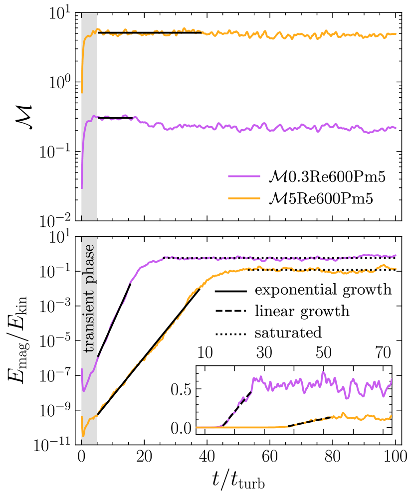
Figure 1: Time evolution of the root-mean-squared sonic Mach number (top panel) and the ratio of the volume-integrated magnetic to kinetic energy (bottom panel) for $\mathcal{M}$0.3Re600Pm5 (purple) and $\mathcal{M}$5Re600Pm5 (yellow). Both plasmas have $\mbox{Re}=600$ and $\mbox{Pm}=5$, but $\mathcal{M}=0.3$ and $5$, respectively. We indicate four distinct phases in the simulations: (1) a transient phase where the turbulent velocity field becomes fully established (grey shaded region); (2) a kinematic phase when the magnetic field grows exponentially in time (black solid lines show exponential model fits); (3) a linear growth phase that begins once magnetic fields are strong enough to suppress some of the kinetic motions (dashed black lines in the inset panel show linear fits); (4) a saturated phase that begins once the magnetic energy is close to equipartition with the kinetic energy (dotted horizontal lines). We report the measured exponential growth rate, and saturated energy ratio for each of our simulation setups in columns (8) and (9) of Table 1, respectively.

In Figure 1 we plot the time evolution of the rms $\mathcal{M}$ and volume-integrated ratio of magnetic to kinetic energy,

$$E_{\mathrm{ratio}}\equiv\frac{E_{\mathrm{mag}}}{E_{\mathrm{kin}}}=\frac{\displaystyle\int_{\mathcal{V}}b^{2}/(8\pi)\,\mathrm{d}\mathcal{V}}{\displaystyle\int_{\mathcal{V}}\rho u^{2}/2\,\mathrm{d}\mathcal{V}}$$ (11)

for two representative simulations, $\mathcal{M}$0.3Re600Pm5 in purple and $\mathcal{M}$5Re600Pm5 in yellow. These runs have identical dimensionless plasma numbers, $\mbox{Re}=600$ with $\mbox{Pm}=5$, but differ in $\mathcal{M}$. In both simulations shown, and in fact for all our simulations (see Table 1), we identify four distinct phases: a transient phase at the start of the simulation, immediately followed by the exponential-growth (kinematic), linear-growth, and finally saturated dynamo phase.

The transient phase roughly spans $0\leq t/t_{\mathrm{turb}}\leq 5$, and is associated with the time it takes for the forcing field to accelerate the plasma into a fully developed (statistically stationary) state. During this transient time, the magnetic field reorganises itself out of this initial configuration, and in the case of subsonic turbulence, into a self-similar configuration that has most of its energy concentrated on the smallest scales (e.g., Fundamental Scales I and Beattie et al. 2023). This reorganisation leads to a short-lived decay in $E_{\mathrm{mag}}$.

During the kinematic phase, $E_{\mathrm{mag}}$ grows exponentially fast, amplifying the magnetic energy by more than 7 orders of magnitude, until it reaches $\sim 10\%$ of the kinetic energy. We measure the growth rate, $\gamma$, of magnetic energy during this phase by fitting each simulation with an exponential model, $E_{\mathrm{mag}}(t)\sim\exp(\gamma t)$, over the time range $5t_{\mathrm{turb}}\leq t\leq t_{\mathrm{end}}$, where $t_{\mathrm{end}}$ is implicitly defined by $E_{\mathrm{ratio}}(t_{\mathrm{end}})=10^{-2}$. For the two simulation show, namely $\mathcal{M}$0.3Re600Pm5 and $\mathcal{M}$5Re600Pm5, we measure growth rates $\gamma=(1.00\pm 0.01)t_{\mathrm{turb}}^{-1}$ and $\gamma=(0.44\pm 0.01)t_{\mathrm{turb}}^{-1}$, and report the measured $\gamma$ for all simulations in column 8 of Table 1. Inspection of these values supports the idea that at fixed Re and Pm, $\gamma$ is generally lower in supersonic compared with subsonic SSDs (Federrath et al., 2011; Schober et al., 2012; Federrath et al., 2014; Chirakkara et al., 2021). During this (kinematic) phase we also confirm that $\mathcal{M}$ remains statistically stationary, and within $5\%$ of our desired value for all our simulations; $\mathcal{M}=0.31\pm 0.01$ for $\mathcal{M}$0.3Re600Pm5, and $\mathcal{M}=5.0\pm 0.2$ for $\mathcal{M}$5Re600Pm5 (see column 7 of Table 1 for all other simulations).

Following the kinematic phase, the magnetic energy growth transitions from an exponential-in-time process to a linear-in-time process for both $\mathcal{M}<1$ and $\mathcal{M}\geq 1$ SSDs. To illustrate this, we plot $E_{\mathrm{ratio}}$ for our two representative simulations on a linear-linear scale in the inset axis of the bottom panel in Figure 1. For our $\mathcal{M}\geq 1$ SSDs, we do not find a transition into quadratic growth, as has been suggested should be the case by Schleicher et al. (2013). Moreover, as was the case in the kinematic phase, we find that the growth rate in the linear-growth regime is lower for the supersonic, i.e., $\mathcal{M}$5Re600Pm5, compared with the subsonic, i.e., $\mathcal{M}$0.3Re600Pm5, SSDs. Finally, once the magnetic energy approaches equipartition with the kinetic energy, the energy ratio saturates, and is maintained thereafter at a nearly constant value by the forcing field; this defines the saturated phase. We measure $(E_{\mathrm{ratio}})_{\mathrm{sat}}=0.43\pm 0.05$ and $0.07\pm 0.01$ for $\mathcal{M}$0.3Re600Pm5 and $\mathcal{M}$5Re600Pm5, respectively, and report this ratio for all simulations in column 9 of Table 1. Again, these values are generally smaller in the supersonic compared with subsonic regimes.

3.2 Magnetic Structures

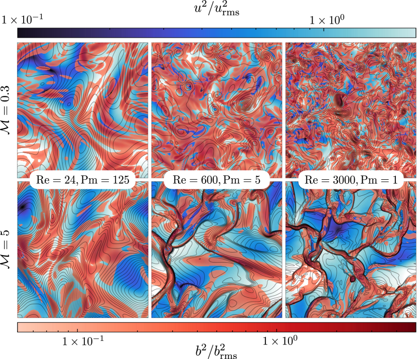
Figure 2: Two-dimensional slices of $u^{2}/u_{\mathrm{rms}}^{2}$ (blue), $b^{2}/b_{\mathrm{rms}}^{2}$ (red), and $\rho/\rho_{\mathrm{rms}}$ (black contours) fields for six different simulations at $N_{\mathrm{res}}^{3}=576^{3}$, spanning a range of plasma regimes. Note that the colourbar for $b^{2}/b_{\mathrm{rms}}^{2}$ is transparent for values $b^{2}/b_{\mathrm{rms}}^{2}<0.5$, so regions of low magnetic energy density are not visible. The six simulations shown are $\mathcal{M}$0.3Re24Pm125, $\mathcal{M}$0.3Re600Pm5, and $\mathcal{M}$0.3Re3000Pm1 in the top row, and $\mathcal{M}$5Re24Pm125, $\mathcal{M}$5Re600Pm5, and $\mathcal{M}$5Re3000Pm1 in the bottom row, respectively, where all simulations have $\mbox{Rm}=3000$, with Pm (and therefore also Re) changing, and velocity flows are subsonic ($\mathcal{M}=0.3$) in the top row and supersonic ($\mathcal{M}=5$) in the bottom row. We see that in the viscous flow regime ($\mbox{Re}<\mbox{Re}_{\mathrm{crit}}\approx 100$; left column), both the subsonic and supersonic simulations produce similar, large-scale magnetic structures. Moving towards the turbulent regime ($\mbox{Re}\gg\mbox{Re}_{\mathrm{crit}}$; middle and right columns), structures that carry most of the magnetic field energy live on significantly smaller scales compared with the viscous regime. In the subsonic regime (top row), magnetic fields are more uniformly distributed and space-filling, occupying even smaller scales than in the corresponding supersonic simulations (bottom row). In the supersonic simulations, magnetic fields are concentrated in high-density shocked regions bounded by sharp jumps in the velocity magnitude, with an almost constant characteristic length of approximately $\ell_{\mathrm{turb}}$, and shock width $\ell_{\mathrm{shock}}$ decreasing with increasing Re.

Now that we have confirmed we observe SSD growth in all of our simulations, we turn our attention to field morphologies during the kinematic phase. In Figure 2 we plot 2D field slices for six simulations from Table 1 (with the two simulations in Figure 1 plotted in the two middle column-panels). All slices are taken from the middle of the simulation domain, $(x,y,z=\ell_{\mathrm{box}}/2)$, at a time realisation midway through the kinematic phase, viz. $(5+t_{\mathrm{end}})/2$, where $t_{\mathrm{end}}$ is defined as in the previous section. The top and bottom row panels show slices for simulations in two different $\mathcal{M}$ regimes, where the top row shows subsonic simulations with $\mathcal{M}=0.3$, and the bottom row shows supersonic simulations with $\mathcal{M}=5$. For all simulations in this figure, we keep $\mbox{Rm}=3000$ fixed, and vary Pm (and thereby Re, or more explicitly $\nu$) between the columns.

In the left column we show two simulations in the viscous-flow regime, where $\mbox{Re}=24<\mbox{Re}_{\mathrm{crit}}$, in the middle column we show mildly turbulent flows, $\mbox{Re}=600\gtrsim\mbox{Re}_{\mathrm{crit}}$, and the right column we show highly turbulent flows, $\mbox{Re}=3000\gg\mbox{Re}_{\mathrm{crit}}$. In each panel we plot $|u^{2}/u_{\mathrm{rms}}^{2}|$ in blue, $|b^{2}/b_{\mathrm{rms}}^{2}|$ in red, and $\rho/\rho_{\mathrm{rms}}$ contours in black, where we have normalised both the velocity and magnetic fields by their rms values to reveal the underlying structure. We truncate the magnetic energy colourbar to show only regions where $|b^{2}/b_{\mathrm{rms}}^{2}|>0.5$, so that the weak-field regions are not shown.

Qualitatively, the top row of Figure 2 illustrates how magnetic field energy shifts from being primarily present in large-scale structures in viscous flows, to smaller scale structures in turbulent flows. This systematic transition is expected during the kinematic phase of a subsonic SSD, where magnetic fields become stretched, folded, and ultimately organised with most of their energy concentrated at the smallest available scales allowed by Ohmic dissipation, $\ell_{\mathrm{p}}\sim\ell_{\eta}\sim\mbox{Re}^{-3/4}\mbox{Pm}^{-1/2}$ (e.g., Schekochihin et al. 2004 and Fundamental Scales I).

In the supersonic regime (bottom row), however, we observe a different transition in the magnetic field morphology. In the viscous regime (left column), both the subsonic and supersonic plasmas have similarly large-scale magnetic structures, but, then in the highly turbulent regime (right column), these two flow regimes look distinctively different. The turbulent, subsonic plasma (top-right panel of Figure 2) appears to have significantly more small-scale magnetic energy structures compared with the turbulent, supersonic plasma, which appears to have its magnetic energy primarily concentrated in elongated, coherent, shocked regions of gas (e.g., illustrated by the tightly-packed density contours that coincide with the boundaries of regions of strong magnetic energy in the bottom-right panel of Figure 2).

While systematic studies of the volume-averaged SSD properties (i.e., growth rate and saturated energy ratio) have explored this transition (Federrath et al., 2011; Chirakkara et al., 2021), no direct, systematic study of the underlying magnetic field properties has been performed, and therefore we focus the remainder of this study on it.

3.3 Measuring Characteristic Scales from Energy Spectra

In the previous section we highlighted the systematic shift of magnetic energy structures from large scale for viscous flows to smaller scale for turbulent flows, which we broadly observed for both subsonic and supersonic plasmas in the kinematic phase of the SSD. To quantify this transition in all of simulations, we measure three characteristic wavenumbers, namely $k_{\nu}$, $k_{\eta}$, and $k_{\mathrm{p}}$, which are directly related ($k\equiv 2\pi/\ell$) to $\ell_{\nu}$, $\ell_{\eta}$, and $\ell_{\mathrm{p}}$, respectively.

In Fundamental Scales I we measured these characteristic wavenumbers by fitting semi-analytical models for the kinetic and magnetic energy spectra, $E_{\mathrm{kin}}(k)$ and $E_{\mathrm{mag}}(k)$, respectively, to 1D shell-integrated power spectra calculated from simulations in the usual way (by summing the total power in discrete, radial shells in k-space). Namely, the energy spectrum of field $\mathrm{{\mn@boldsymbol{\mathit{\psi}}}}$ is computed as

$$E_{\psi}(k,t)=\sum_{k^{*}<|\mathrm{{\mn@boldsymbol{\mathit{k}}}}|<k^{*}+\Delta k^{*}}4\pi k^{2}\widetilde{\psi}(\mathrm{{\mn@boldsymbol{\mathit{k}}}},t)\,\widetilde{\psi}^{*}(\mathrm{{\mn@boldsymbol{\mathit{k}}}},t)$$ (12)

where we choose to bin in integer $k$-bins ($k^{*}\in\mathds{Z}^{+}:k^{*}\neq 0$) separated by $\Delta k^{*}=1$, and

$$\widetilde{\psi}(\mathrm{{\mn@boldsymbol{\mathit{k}}}},t)=\frac{1}{(2\pi\ell_{\mathrm{box}})^{3/2}}\int_{\mathcal{V}}\mathrm{{\mn@boldsymbol{\mathit{\psi}}}}(\mathrm{{\mn@boldsymbol{\mathit{\ell}}}},t)\exp\left(-i\mathrm{{\mn@boldsymbol{\mathit{k}}}}\cdot\mathrm{{\mn@boldsymbol{\mathit{\ell}}}}\right)\,\mathrm{d}^{3}\ell$$ (13)

is the Fourier transform of $\psi(\mathrm{{\mn@boldsymbol{\mathit{\ell}}}},t)$, with $\widetilde{\psi}^{*}(\mathrm{{\mn@boldsymbol{\mathit{k}}}},t)$ its complex conjugate.

We also attempted this approach for the present study, but found that the existing functional models for both energy spectra failed to reliably measure characteristic scales for our supersonic simulations, especially our lower-resolution runs, which are required to perform our resolution study. More specifically, due to the limited inertial range for our low-Re simulations, we could not effectively constrain $k_{\nu}$, and found that $E_{\mathrm{mag}}(k)$, for our supersonic simulations, had a wider energy spectrum than the subsonic simulations, which was not well-fit by the functional form used in Fundamental Scales I for the subsonic case. Prompted by these challenges, we develop new and simpler, spectral model-free methods for measuring $k_{\nu}$, $k_{\eta}$, and $k_{\mathrm{p}}$, based on the underlying turbulence and fluid theory, which we apply to all our simulations, and demonstrate yield robust results through all of our flow regimes.

3.3.1 Characteristic Viscous Dissipation Wavenumber

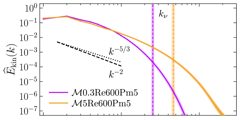
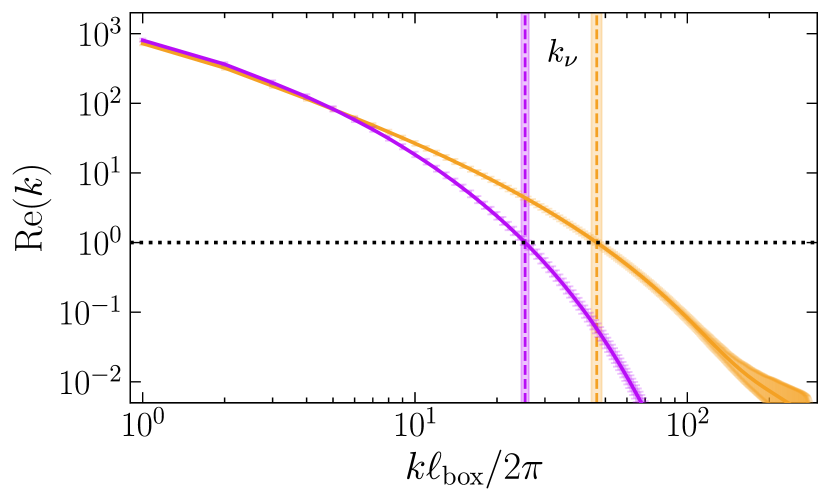
Figure 3: Normalised and time-averaged (over the kinematic phase) kinetic energy spectrum ($\widehat{E}_{\mathrm{kin}}(k)$; top panel) constructed with $\mathrm{{\mn@boldsymbol{\mathit{\psi}}}}=\mathrm{{\mn@boldsymbol{\mathit{u}}}}/\sqrt{2}$ in Equation 13, for the $\mathcal{M}$0.3Re600Pm5 (purple) and $\mathcal{M}$0.3Re600Pm5 (yellow) simulations run at $N_{\mathrm{res}}^{3}=576^{3}$. The solid lines shows the $50^{\rm th}$ percentile of the $\widehat{E}_{\mathrm{kin}}(k)$ spectrum over all snapshots during this phase, and the bands show the $16^{\rm th}$ to $84^{\rm th}$ percentile variance of $\widehat{E}_{\mathrm{kin}}(k)$. We also plot the wavenumber-dependent hydrodynamic Reynolds number ($\mbox{Re}(k)$; bottom panel), Equation 14. From $\mbox{Re}(k)$ we measure a characteristic kinetic energy dissipation (viscous) wavenumber, $k_{\nu}:\mbox{Re}(k_{\nu})=1$ (via Equation 16), which we annotate with vertical lines for both simulations in the top and bottom panels. For reference, we also plot $\widehat{E}_{\mathrm{kin}}(k)\sim k^{-5/3}$ and $\widehat{E}_{\mathrm{kin}}(k)\sim k^{-2}$ in the top panel, which corresponds with the expected inertial range scaling of Kolmogorov (1941) and Burgers (1948) kinetic energy spectra, respectively.

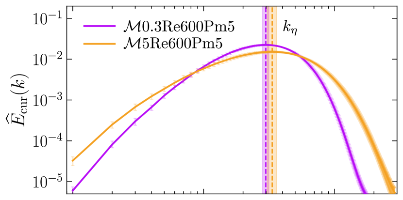
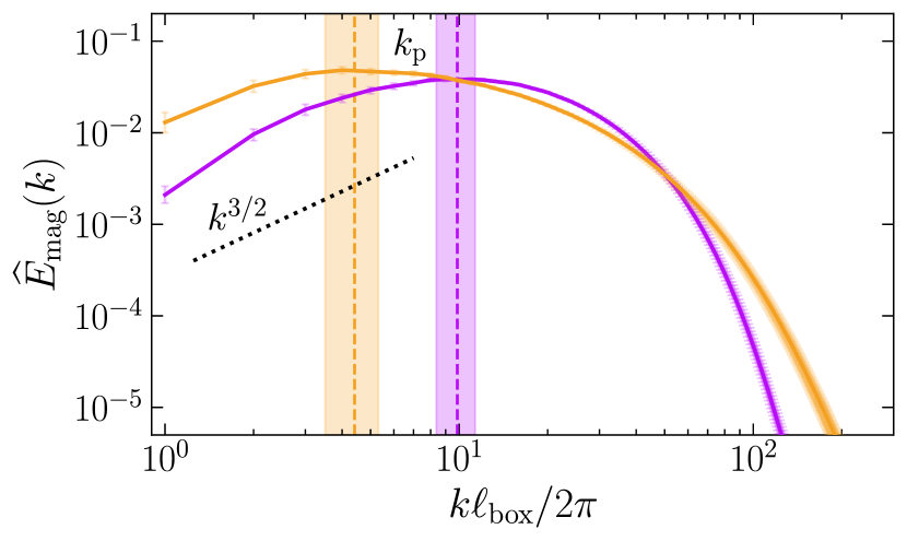
Figure 4: As in Figure 3, but for the current density power spectra ($\widehat{E}_{\mathrm{cur}}(k)$; top panel) and magnetic energy spectrum ($\widehat{E}_{\mathrm{mag}}(k)$; bottom panel) for $\mathcal{M}$0.3Re600Pm5 and $\mathcal{M}$5Re600Pm5. We annotate the measured characteristic magnetic dissipation (resistive) wavenumber in the top panel, $k_{\eta}$ (Equation 17), and the magnetic peak wavenumber, $k_{\mathrm{p}}$ (Equation 18), in the bottom panel. We also annotate $\widehat{E}_{\mathrm{mag}}(k)\sim k^{3/2}$ for reference, which is the expected scaling of $E_{\mathrm{mag}}(k)$ in the subviscous range during the kinematic phase of a subsonic SSD (Kazantsev, 1968; Schekochihin et al., 2002a).

We define the turbulent viscous wavenumber, $k_{\nu}$, directly from the definition in Kolmogorov turbulence, i.e., the wavenumber where the scale-dependent hydrodynamic Reynolds number equals one, $\mbox{Re}(k_{\nu})=1$. This scale marks the transition from inertial forces dominating in the turbulent cascade, $k_{\mathrm{turb}}<k<k_{\nu}$, to dissipation dominating at $k_{\nu}<k$. Hence, to measure $k_{\nu}$, we construct the wavenumber-dependent hydrodynamic Reynolds number,

$$\mbox{Re}(k,t)=\frac{u_{\mathrm{turb}}(k,t)}{\nu k},$$ (14)

which follows from the turbulent velocity as a function of $k$,

$$u_{\mathrm{turb}}(k,t)=\left(\frac{2}{\rho_{0}}\int_{k}^{\infty}E_{\mathrm{kin}}(k^{\prime},t)\,\mathrm{d}k^{\prime}\right)^{1/2}.$$ (15)

In practice we solve for $k_{\nu}$ from our simulations using a root finding method,

$$k_{\nu}(t)=\texttt{argmin}_{k}\Big{[}\mathcal{I}\Big{\{}\Big{|}\mbox{Re}(k,t)-1\Big{|}\Big{\}}\Big{]},$$ (16)

where $|\dots|$ is the absolute operator, $\mathcal{I}[\dots]$ is a piecewise cubic polynomial (spline) interpolation operator, as performed in Beattie et al. (2023), and $\texttt{argmin}_{k}[h(k)]$ returns the argument $k$ which minimises the function $h(k)$. For each of our simulations, we evaluate Equation 16 at each time-snapshot during the kinematic phase.

While Equation 16 provides a simple way of extracting the viscous wavenumber from $E_{\mathrm{kin}}(k)$, there remains the question of which field, $\mathrm{{\mn@boldsymbol{\mathit{\psi}}}}$, to Fourier transform in the supersonic regime. When $\mathrm{{\mn@boldsymbol{\mathit{\psi}}}}=\mathrm{{\mn@boldsymbol{\mathit{u}}}}/\sqrt{2}$ in Equation 13, then $E_{\mathrm{kin}}(k)$ is the velocity power spectrum – which in incompressible flows is directly proportional to the kinetic energy spectrum because the density field is constant – and Equation 14 then carries the same units as the usual definition of the hydrodynamic Reynolds number, i.e., Equation 8 is computed from the velocity on scale $\ell$. However, this velocity power spectrum definition for $E_{\mathrm{kin}}(k)$ ignores the covariance between the density field and the square velocity field, i.e., $\left\langle\rho u^{2}\right\rangle_{\mathcal{V}}/2$ (see footnote 3), as well as fluctuations in the density field, which in isothermal plasmas are a factor of $\mathcal{M}^{2}$ larger than velocity fluctuations (this factor follows from a unit analysis of the ideal-hydrodynamic momentum equation in steady state). Beattie & Federrath (2020) showed that the density spectrum becomes dominated by high-$k$ modes that can lead to large pressure gradients, which mediate the exchange of kinetic and internal energy (see for example Federrath et al., 2010; Federrath, 2013; Schmidt & Grete, 2019; Grete et al., 2021, 2023). Therefore we also check whether density fluctuations affect our measurements of $k_{\nu}$, by also considering the definition for $E_{\mathrm{kin}}$ which carries the units of kinetic energy, namely with $\mathrm{{\mn@boldsymbol{\mathit{\psi}}}}=\mathrm{{\mn@boldsymbol{\mathit{u}}}}\sqrt{\rho/2}$ (see, e.g., Federrath et al., 2010; Grete et al., 2021, 2023).

Here in the main text we focus on $k_{\nu}$ derived from Equation 14 constructed with $\mathrm{{\mn@boldsymbol{\mathit{\psi}}}}=\mathrm{{\mn@boldsymbol{\mathit{u}}}}/\sqrt{2}$, which we demonstrate in Figure 3 for the same two representative simulations shown in Figure 1, namely $\mathcal{M}$0.3Re600Pm5 and $\mathcal{M}$5Re600Pm5. Then in Appendix A we demonstrate that regardless of the choice of definition for $E_{\mathrm{kin}}(k)$, whether based on $\mbox{Re}(k)$ having dimensionless units (i.e., constructed with $\mathrm{{\mn@boldsymbol{\mathit{\psi}}}}=\mathrm{{\mn@boldsymbol{\mathit{u}}}}/\sqrt{2}$), or choosing $\mathrm{{\mn@boldsymbol{\mathit{\psi}}}}=\mathrm{{\mn@boldsymbol{\mathit{u}}}}\sqrt{\rho/2}$ such that $E_{\mathrm{kin}}(k)$ carries units of kinetic energy, we recover the same scaling behaviour for $k_{\nu}$, and thus the choice of definition for $E_{\mathrm{kin}}$ does not any of the conclusion presented in our study.

3.3.2 Characteristic Resistive Dissipation Wavenumber

While our approach of defining $k_{\nu}$ in terms of the wavenumber-dependent hydrodynamic Reynolds number performs well, we find that an analogous approach to defining the resistive wavenumber in terms of the spectrum of Rm yields results that are inconsistent with those derived from early methods (Kulsrud & Anderson, 1992; Kriel et al., 2022; Brandenburg et al., 2023); see Appendix B for details. For this reason we adopt a different approach by recognising that, since we employ Ohmic dissipation in the induction equation (Equation 3), the Ohmic dissipation rate at any point in space is exactly equal to $\eta j^{2}$. On this basis we define the resistive wavenumber as the wavenumber of maximum $j^{2}(k)$, corresponding to the maximum magnetic dissipation (since $\eta$ is a constant). Explicitly, we define $k_{\eta}$ as the value of $k$ corresponding to the maximum of the 1D shell-integrated current density spectrum (which has units of current density squared), $E_{\mathrm{cur}}(k)$, which is defined similarly to $E_{\mathrm{kin}}(k)$ in Section 3.3.1, but for the field $\mathrm{{\mn@boldsymbol{\mathit{\psi}}}}=\nabla\times\mathrm{{\mn@boldsymbol{\mathit{b}}}}/(4\pi)$.

In practice we implement this as

$$k_{\eta}(t)=\texttt{argmax}_{k}\Big{[}\mathcal{I}\Big{\{}E_{\mathrm{cur}}(k,t)\Big{\}}\Big{]},$$ (17)

where $\mathcal{I}\{\dots\}$ is defined as in Equation 16, and $\texttt{argmax}_{k}[h(k)]$ returns the argument $k$ which maximises $h(k)$. As with $k_{\nu}$, we compute this quantity for every snapshot during the kinematic phase. We illustrate this procedure in the top panel of Figure 4, where in analogy with the top panel of Figure 3, we plot the normalised and time-averaged (over the kinematic phase) $E_{\mathrm{cur}}$ for our two representative simulations, with the corresponding resistive wavenumbers $k_{\eta}$ indicated by vertical bands.

3.3.3 Peak Magnetic Wavenumber

Finally, we define the magnetic peak wavenumber as the maximum of $E_{\mathrm{mag}}(k)$, defined similarly to the current density power spectra but with $\mathrm{{\mn@boldsymbol{\mathit{\psi}}}}=\mathrm{{\mn@boldsymbol{\mathit{b}}}}/{8\pi}$. Explicitly,

$$k_{\mathrm{p}}(t)=\texttt{argmax}_{k}\Big{[}\mathcal{I}\Big{\{}E_{\mathrm{mag}}(k,t)\Big{\}}\Big{]}.$$ (18)

We illustrate $E_{\mathrm{mag}}(k)$ and $k_{\mathrm{p}}$ for our two representative simulations in the bottom panel of Figure 4. In Appendix C we point out that, while the magnetic correlation wavenumber is directly proportional to peak wavenumber during the kinematic phase of a subsonic (both viscous and turbulent) SSD (Schekochihin et al., 2004; Galishnikova et al., 2022; Beattie et al., 2023), this scaling breaks down for supersonic, turbulent SSDs.

3.4 Convergence of Measured Wavenumbers

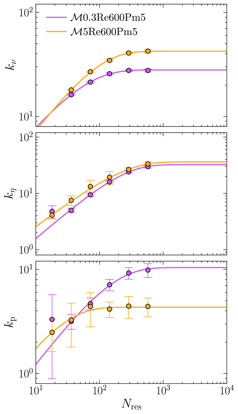
Figure 5: Measured viscous ($k_{\nu}$; top panel), resistive ($k_{\eta}$; middle panel), and magnetic peak ($k_{\mathrm{p}}$; bottom panel) wavenumbers plotted against linear grid resolution for $\mathcal{M}$0.3Re600Pm5 (magenta) and $\mathcal{M}$5Re600Pm5 (yellow). We overlay a best-fit of our convergence model, Equation 19, to each set of wavenumbers to measure characteristic wavenumbers that have converged with resolution. We report the converged $k_{\nu}$, $k_{\eta}$, and $k_{\mathrm{p}}$ for each of our simulations in columns (10), (11), and (12) of Table 1, respectively.

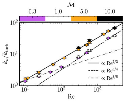
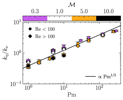
Figure 6: For each of our simulation setups in Table 1, we compare the converged viscous wavenumber, $k_{\nu}$, with the hydrodynamic Reynolds number of the plasma flow (left panel). We also plot the scale separation between the magnetic and kinetic dissipation wavenumbers, $k_{\eta}/k_{\nu}$, with the magnetic Prandtl number (right panel). We colour points based on their $\mathcal{M}$, where $\mathcal{M}=0.3$ is coloured magenta, $\mathcal{M}=1$ is coloured white, $\mathcal{M}=5$ is coloured yellow, and $\mathcal{M}=10$ is coloured black. To guide the eye in the left panel, we show theoretical scalings of $k_{\nu}$ for Burgers (1948): $k_{\nu}\sim\mathrm{Re}^{2/3}$ (solid black line; Schober et al. 2012), Kolmogorov (1941): $k_{\nu}\sim\mathrm{Re}^{3/4}$ (dashed black line), and for a viscous, subsonic velocity field (see Fundamental Scales I): $k_{\nu}\sim\mathrm{Re}^{3/8}$ (dotted black line). In the right panel we annotate a $k_{\eta}/k_{\nu}\sim\mbox{Pm}^{1/2}$ scaling, and plot viscous simulations ($\mbox{Re}<\mbox{Re}_{\mathrm{crit}}\approx 100$) as circles, and turbulent simulations ($\mbox{Re}>\mbox{Re}_{\mathrm{crit}}$) as diamonds.

As previously discussed in Section 2.3, we ensure that all the characteristic wavenumbers we measure from our different simulation setups are converged with respect to the grid resolution $N_{\mathrm{res}}$. We do this by running each simulation setup in Table 1 across a wide range of $N_{\mathrm{res}}$, measuring our three wavenumbers of interest, $k_{\rm scale}\in\{k_{\nu},k_{\eta},k_{\mathrm{p}}\}$ in the kinematic phase, and then fitting a generalised logistic model of the functional form

$$k_{\rm scale}(N_{\mathrm{res}})=k_{\rm scale}(\infty)\left(1-\exp\left\{-\left(\frac{N_{\mathrm{res}}}{N_{\rm res,crit}}\right)^{R}\right\}\right),$$ (19)

to the resolution-dependent wavenumbers. The parameters in our fits are $k_{\rm scale}(\infty)$, which represents the converged ($N_{\mathrm{res}}\to\infty$) value of each wavenumber $\{k_{\nu},k_{\eta},k_{\mathrm{p}}\}$, the rate of convergence $R$, and the critical resolution $N_{\rm res,crit}$ at which characterises the resolution where convergence begins.

As discussed in Section 2.3, we start by running each simulation configuration across $N_{\mathrm{res}}=18-288$, separated by factors of 2, and then we fit those data for $N_{\mathrm{res,crit}}$. If we find that our best-fit value of $N_{\mathrm{res,crit}}$ is larger than 288, or that our data does not yield a fit for $N_{\mathrm{res,crit}}$ with reasonable uncertainty, we rerun that setup at the higher resolution $N_{\mathrm{res}}=576$. We then repeat the convergence test, doubling the resolution until we obtain a well-constrained value of $N_{\mathrm{res,crit}}$, such that our highest-resolution run for each setup satisfies $\texttt{max}[\{N_{\mathrm{res}}\}]>N_{\mathrm{res,crit}}$.

In Figure 5 we plot the resolution ($N_{\mathrm{res}}$) dependent $k_{\nu}$, $k_{\eta}$, and $k_{\mathrm{p}}$, and our best fits to these wavenumbers, for our two representative simulations. Broadly, for both simulations, we find evidence of convergence at $N_{\mathrm{res}}\approx 576$, but since $k_{\nu}$, $k_{\eta}$, and $k_{\mathrm{p}}$ may all exist on different scales, one would expect the convergence properties of each wavenumber to be different, since small-scale (high-$k$) structures are expected to require higher resolution to converge than larger-scale (low-$k$) structures. This is what we find. For $\mathcal{M}$0.3Re600Pm5 we find $k_{\nu}$ begins to converge at $N_{\rm res,crit}=43.0\pm 2.2$, while $k_{\eta}$ and $k_{\mathrm{p}}$ begin converging at $N_{\rm res,crit}=190.4\pm 20.2$ and $N_{\rm res,crit}=117.2\pm 40.0$, respectively. This is expected, since we are operating in the $\mbox{Pm}\geq 1$ regime where magnetic structures are smaller-scale than velocity structures, viz. $k_{\nu}<k_{\eta}\sim k_{\mathrm{p}}$, and therefore require a higher grid resolution to resolve. By contrast, for $\mathcal{M}$5Re600Pm5, we find that $k_{\nu}$ shows convergence at $N_{\rm res,crit}=79.4\pm 4.6$, whereas $k_{\eta}$ requires $N_{\rm res,crit}=173.5\pm 40.7$ and $k_{\mathrm{p}}$ requires $N_{\rm res,crit}=20.6\pm 18.3$. Comparing the subsonic and supersonic cases, it is noteworthy that $k_{\eta}$ shows similar convergence behaviour, but that $k_{\mathrm{p}}$ converges at significantly lower grid resolution, consistent with the visual differences in size scale visible in Figure 2.

We report the converged values $k_{\rm scale}(\infty)$ (extrapolated to infinite resolution) for all our simulations in columns 10–12 of Table 1, and use this in all of our analysis that follows, but for compactness from this point on (and in the header of Table 1) we drop the notation $(\infty)$. We also report the measured $N_{\rm res,crit}$ and $R$ for all our simulations in Table 2. These fits are based on using all data up to the highest resolution we have run for each simulation configuration.

3.5 Where Do Kinetic and Magnetic Fields Dissipate?

Now that we have obtained converged dissipation wavenumbers, we are prepared to explore how these scales depend on the dimensionless plasma parameters $\mathcal{M}$, Re and Pm. In the kinematic phase of the dynamo, where magnetic fields are subdominant on all scales, we expect $k_{\nu}$ to depend only on the kinetic field properties (i.e., $k_{\mathrm{turb}}$ and Re), and the separation between $k_{\nu}$ and $k_{\eta}$ to be a function of only Pm. The exact relationship between these dissipation scales and principal parameters should change between the subsonic and supersonic regimes, an effect we explore in Figure 6, where we plot $k_{\nu}/k_{\mathrm{turb}}$ against Re in the left panel and $k_{\eta}/k_{\nu}$ against Pm in the right panel, in both cases colour-coding the simulations by $\mathcal{M}$.

3.5.1 Viscous Scaling

We first consider the scaling behaviour of $k_{\nu}$, and its dependence on Re, in the left hand panel of Figure 6. Here, for our turbulent ($\mbox{Re}\gtrsim\mbox{Re}_{\mathrm{crit}}$), subsonic ($\mathcal{M}=0.3$; plotted in yellow) and transsonic ($\mathcal{M}=1$; plotted in white) simulations, we recover $k_{\nu}/k_{\mathrm{turb}}\sim\mbox{Re}^{3/4}$ as expected for Kolmogorov (1941) turbulence with $E_{\mathrm{kin}}(k)\sim k^{-5/3}$. This is the same scaling behaviour we had previously demonstrated in Fundamental Scales I using our previous methods, and now, here we confirm that our new method (Equation 16) recovers the same scaling in the same flow regime. This scaling has also been extensively demonstrated in both numerical simulations (Yeung & Zhou, 1997; Schumacher, 2007; Schumacher et al., 2014) and laboratory experiments (Barenblatt et al., 1997).

For our viscous ($\mbox{Re}<\mbox{Re}_{\mathrm{crit}}$), trans- and subsonic ($\mathcal{M}\leq 1$) simulations, we recover $k_{\nu}/k_{\mathrm{turb}}\sim\mbox{Re}^{3/8}=(\mbox{Re}^{3/4})^{1/2}$. This result again agrees broadly with our previous findings in Fundamental Scales I, where we had found that viscous, subsonic flows have sub-Gaussian velocity gradients (viscous dissipation lacked intense, local events), which led to a scaling of $k_{\nu}$ with Re that was shallower than expected for Kolmogorov (1941) turbulence.

Finally, for our supersonic ($\mathcal{M}=5$ and $10$) simulations we measure $k_{\nu}/k_{\mathrm{turb}}\sim\mbox{Re}^{2/3}$, which corresponds with Burgers (1948) turbulence where $E_{\mathrm{kin}}(k)\sim k^{-2}$ (Schober et al., 2012; Federrath et al., 2021), which is a shallower scaling in Re compared with Kolmogorov (1941) turbulence, but steeper than the scaling for a viscous, subsonic velocity field (Fundamental Scales I).

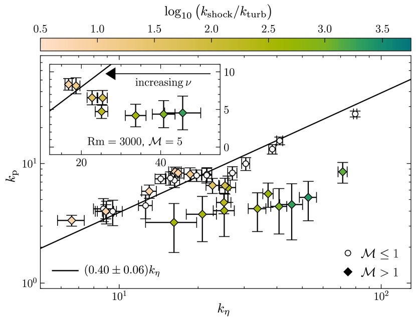
Figure 7: Converged magnetic peak wavenumber, $k_{\mathrm{p}}$, plotted against the converged characteristic magnetic dissipation (resistive) wavenumber, $k_{\eta}$, for each simulation setup in Table 1. In the main panel, we plot sub- and transsonic simulations with white circles, and in both (main as well as inset) panels, we plot supersonic simulations with diamonds that are coloured based on the reciprocal of our characteristic shock width model, $k_{\mathrm{shock}}$ (see Equation 26). To provide further insights into the supersonic dynamics, we add an inset panel where we focus on a subset of the supersonic simulations. In this inset, we plot the set of $\mathcal{M}=5$ simulations where $\mbox{Rm}=3000$ is fixed, and Re is changed via $\nu$. In both panels, we also annotate the same reference $k_{\mathrm{p}}\sim k_{\eta}$ line in black.

To summarise the three regimes concisely,

$$k_{\nu}/k_{\mathrm{turb}}\sim\left\{\begin{matrix}\mbox{Re}^{3/8},&\mathcal{M}\leq 1,&\mbox{Re}<\mbox{Re}_{\mathrm{crit}},\\ \mbox{Re}^{3/4},&\mathcal{M}\leq 1,&\mbox{Re}\geq\mbox{Re}_{\mathrm{crit}},\\ \mbox{Re}^{2/3},&\mathcal{M}>1.\end{matrix}\right.$$ (20)

The fact that during the kinematic phase of our SSD simulations we have in all cases recovered well-known results for purely hydrodynamic turbulence is not surprising, since during the kinematic phase $E_{\mathrm{mag}}(k)\ll E_{\mathrm{kin}}(k)$ for all $k$ (see Beattie et al. 2023 for the sub-sonic $E_{\mathrm{mag}}(k)/E_{\mathrm{kin}}(k)$ functions showing this), and therefore the magnetic field exerts a negligible Lorentz force. Thus Equation 2 becomes independent of $\mathrm{{\mn@boldsymbol{\mathit{b}}}}$, and approximately hydrodynamical. Once $\mathrm{{\mn@boldsymbol{\mathit{b}}}}$ is strong enough (as the dynamo process transitions into the linear growth and saturated regimes), we do not expect these dissipation scalings to persist, but measuring these scalings is beyond the scope of the current study.

3.5.2 Resistive Scaling

Next, in the right hand panel of Figure 6, we consider the scale-separation between $k_{\nu}$ and $k_{\eta}$, and how this scale separation depends upon Pm. This is the most direct way to test whether, even in supersonic flows, the smallest scale kinetic eddies are responsible for amplifying (shearing) magnetic fields (see Section 2.2.3 for details). And in fact, we find evidence that regardless of the flow regime, $k_{\eta}/k_{\nu}$ scales like $\mbox{Pm}^{1/2}$, which implies that this is the case.

Now, perhaps this is not completely unexpected. At no stage during the derivation for the theoretical $k_{\eta}\sim k_{\nu}\mbox{Pm}^{1/2}$ expectation does one make any assumption about the underlying properties of the velocity field (i.e., if the flow is turbulent or viscous, subsonic or supersonic), as long as the flow is isotropic. Namely, Schekochihin et al. (2002b) put forward $\ell_{\eta}\sim\ell_{\nu}\,\mbox{Pm}^{-1/2}$ by assuming that $E_{\mathrm{mag}}$ is primarily grown by viscous eddies, with characteristic shearing (or stretching) rate $u_{\nu}/\ell_{\nu}$ (where $u_{\nu}$ is the velocity on scale $\ell_{\nu}$). Balancing this rate of energy injection into the magnetic field with the rate of Ohmic dissipation, $\eta/\ell_{\eta}^{2}$, rearranges to give

$$\ell_{\eta}\sim\left(\frac{\eta\,\ell_{\nu}}{u_{\nu}}\right)^{1/2}=\left(\frac{\eta}{\nu}\frac{\nu}{u_{\nu}}\ell_{\nu}\right)^{1/2}\sim\ell_{\nu}\,\mbox{Pm}^{-1/2},$$ (21)

where $\ell_{\nu}\sim\nu/u_{\nu}$ follows from a straightforward unit analysis.

From this we conclude that $k_{\eta}\sim k_{\nu}\,\mbox{Pm}^{1/2}$ is a universal scaling in the $\mbox{Pm}\geq 1$ regime, a result that favours a picture in which the smallest scale (viscous) eddies are responsible for converting $E_{\mathrm{kin}}$ into $E_{\mathrm{mag}}$, completely invariant to whether the kinetic energy cascade is Burgers (1948)-like or Kolmogorov (1941)-like, and moreover, turbulent ($\mbox{Re}>\mbox{Re}_{\mathrm{crit}}$) or viscous ($\mbox{Re}<\mbox{Re}_{\mathrm{crit}}$).

3.6 What Sets the Peak Magnetic Energy Scale?

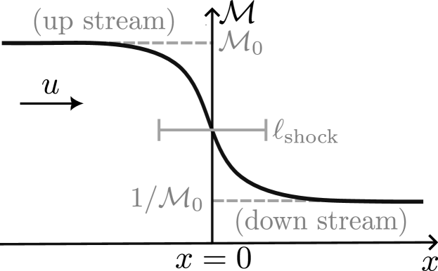
Figure 8: Schematic of a 1D velocity shock, in the reference frame of the shock: the up stream material ($x<0$) with up stream sonic Mach number $\mathcal{M}_{0}$ approaches the shock located at $x=0$ with velocity $u$.

In Figure 7 we plot the wavenumber where the magnetic energy spectrum peaks, $k_{\mathrm{p}}$, and compare it with the characteristic resistive wavenumber, $k_{\eta}$, for all of our simulations. We notice an interesting dichotomy in the scaling of $k_{\mathrm{p}}$ derived from the $\mathcal{M}\leq 1$ (sub- and transsonic) and $\mathcal{M}>1$ (supersonic) simulations, and introduce a new colouring criteria for all our simulations to highlight the differences between the different flow regimes. We colour all the $\mathcal{M}\leq 1$ simulations white, and colour the $\mathcal{M}>1$ simulations based on a colour map that we will discuss and motivate below.

Before we move to the supersonic simulations, we again verify that our new methods for measuring $k_{\mathrm{p}}$ and $k_{\eta}$ are robust and reliable. To demonstrate this, we highlight that we find $k_{\mathrm{p}}=(0.40\pm 0.06)\,k_{\eta}$, determined from averaging our $\mathcal{M}\leq 1$ SSD simulations (white points), which recovers $k_{\mathrm{p}}\sim k_{\eta}$. This is a well known theoretical result (e.g.,  Schekochihin et al., 2002b), which was confirmed in previous numerical simulations (Fundamental Scales I; Brandenburg et al. 2023), and tells us that in the kinematic phase of (even approximately) incompressible SSDs, magnetic energy becomes concentrated at the smallest scales allowed by magnetic dissipation (e.g.,  Schekochihin et al., 2002b; Xu & Lazarian, 2016; Kriel et al., 2022; Brandenburg et al., 2023). Notice, however, that the $0.40\pm 0.06$ constant of proportionality in this relation is dependent upon the models used to measure $k_{\mathrm{p}}$ and $k_{\eta}$, and therefore expectantly different from the $1.2\pm 0.2$ found in Fundamental Scales I (see Section 3.3 for a discussion on our new methods).

The behaviour of $k_{\mathrm{p}}$ for supersonic SSDs during the kinematic phase is dramatically different from the subsonic scaling, though. While a portion of our $\mathcal{M}>1$ simulations follow the same $k_{\mathrm{p}}\sim k_{\eta}$ scaling as the subsonic cases, the rest deviate significantly to wavenumbers such that $k_{\mathrm{p}}<k_{\eta}$. To develop an intuition for why this happens, we briefly turn our attention back to the bottom row panels in Figure 2, which show runs $\mathcal{M}$5Re24Pm125, $\mathcal{M}$5Re600Pm5, and $\mathcal{M}$5Re3000Pm1, respectively. For $\mathcal{M}$5Re3000Pm1, for example, magnetic energy (red) seems to be preferentially concentrated inside of shocked regions of gas, where there are large jumps in the density field (black contours), which have previously been shown to be coherent up to $k_{\mathrm{turb}}$ (and even beyond, depending upon how strong the magnetisation is; Beattie & Federrath 2020; Beattie et al. 2021), even though they fill very little of the volume (e.g., Hopkins, 2013; Robertson & Goldreich, 2018; Mocz & Burkhart, 2019; Beattie et al., 2022b). Based on $k_{\mathrm{p}}$, the shocks do not seem to be present in $\mathcal{M}$5Re24Pm125, where even though the velocity dispersion is large ($u_{\mathrm{turb}}\gtrsim 5c_{\mathrm{s}}$), the kinetic energy diffusion coefficient, $\nu$, is large enough to dissipate the supersonic velocities before they are able to form shocks. A likely criteria for this effect is that the shock lifetime, $t_{\mathrm{shock}}$ (which is a fraction of the sound crossing time across the shocked region; Robertson & Goldreich 2018), is shorter than the diffusion timescale, $t_{\nu}\sim\ell_{\nu}^{2}/\nu$.

Our supersonic simulations appear to support a hypothesis that, when shocks are present, $\ell_{\mathrm{p}}$ approaches a value much larger than $\ell_{\eta}$, that depends somehow on the typical width of shocks, $\ell_{\mathrm{shock}}$. To test this conjecture, we estimate $\ell_{\mathrm{shock}}$ from the quasi-equilibrium state of the momentum equation, omitting the magnetic terms because the Lorentz force is unimportant in the kinematic dynamo phase, even in shocked regions ($E_{\mathrm{mag}}(k)/E_{\mathrm{kin}}(k)\ll 1,$ for all $k$; Beattie et al. 2023), and excluding external forcing, but not setting viscosity or the sound speed to zero (e.g., the pressureless, Burgers’ equation limit, $\nabla P/\mathcal{M}^{2}\rightarrow 0$ as $\mathcal{M}\rightarrow\infty$), namely,

$$\nabla\cdot\left(\rho\mathrm{{\mn@boldsymbol{\mathit{u}}}}\otimes\mathrm{{\mn@boldsymbol{\mathit{u}}}}+c_{\mathrm{s}}^{2}\rho\textbf{{I}}-2\nu\rho\textbf{{S}}\right) =0.$$ (22)

Since shocks are generated isotropically in our supersonic turbulent simulations, we simplify Equation 22 by considering a single characteristic shock travelling in 1D (adopting the usual convention that $x<0$ and $x>0$ are the up and down stream directions, respectively; see Figure 8 for a schematic of this setup). It follows that

$$\frac{\mathrm{d}}{\mathrm{d}x}\left[\rho u^{2}+c_{\mathrm{s}}^{2}\rho-\frac{4\nu\rho}{3}\frac{\mathrm{d}u}{\mathrm{d}x}\right]=0.$$ (23)

The quantity in square brackets is the momentum flux, which is conserved across the shock, and since $\mathrm{d}u/\mathrm{d}x\to 0$ as $x\to-\infty$ (i.e., the velocity gradient vanishes far up stream of the shock), this momentum flux must be $\rho_{0}u_{0}^{2}+c_{s}^{2}\rho_{0}$, where subscript 0 indicates quantities in the far up stream region. Conservation of mass flux further implies that $\rho u=\rho_{0}u_{0}=\mathrm{const}$, and making use of this result allows us to rewrite Equation 23 in the form

$$\frac{\mathrm{d}\mathcal{M}}{\mathrm{d}x}=\frac{3c_{\mathrm{s}}}{4\nu}\left(\mathcal{M}^{2}-\left(\frac{\mathcal{M}_{0}^{2}+1}{\mathcal{M}_{0}}\right)\mathcal{M}+1\right),$$ (24)

where $\mathcal{M}=u/c_{\mathrm{s}}$ is the position-dependent sonic Mach number.

Equation 24 has the form of a Riccati equation (nonlinear, quadratic differential equation of first-order) with constant coefficients, and has the solution that $\mathrm{d}\mathcal{M}/\mathrm{d}x=0$ when $\mathcal{M}=\mathcal{M}_{0}$ or $1/\mathcal{M}_{0}$; the former possibility represents the up stream region, and the latter the down stream region. Since $x$ does not explicitly appear on the right-hand side of Equation 24, we are free to choose our coordinate system such that $\mathcal{M}=1$ at $x=0$ (as we have done in Figure 8). From this, we estimate the characteristic shock width as

$$\frac{\ell_{\mathrm{shock}}}{\ell_{\mathrm{turb}}}\sim\frac{1}{\ell_{\mathrm{turb}}}\left[\frac{\mathcal{M}}{\mathrm{d}\mathcal{M}/\mathrm{d}x}\right]_{x=0}\sim\frac{\mathcal{M}_{0}^{2}}{\mbox{Re}\,(\mathcal{M}_{0}-1)^{2}}.$$ (25)

In supersonic turbulence one expects to see a population of shocks that take on a wide distribution of $\ell_{\mathrm{shock}}$ (e.g.,  Smith et al., 2000; Brunt & Heyer, 2002; Donzis, 2012; Lesaffre et al., 2013; Squire & Hopkins, 2017; Park & Ryu, 2019; Beattie et al., 2020; Beattie et al., 2022b), where each of the different $\ell_{\mathrm{shock}}$ are determined by the $\mathcal{M}_{0}$ that is up stream from it. That being said, the distribution of shock widths is controlled by the turbulent properties on $\ell_{\mathrm{turb}}$, where on average, $\mathcal{M}_{0}\approx\mathcal{M}$. Therefore, we model the characteristic width of a shock in our isotropic turbulent simulations as

$$\frac{k_{\mathrm{turb}}}{k_{\mathrm{shock}}}=\frac{\ell_{\mathrm{shock}}}{\ell_{\mathrm{turb}}}\sim\frac{\mathcal{M}^{2}}{\mbox{Re}\,(\mathcal{M}-1)^{2}}.$$ (26)

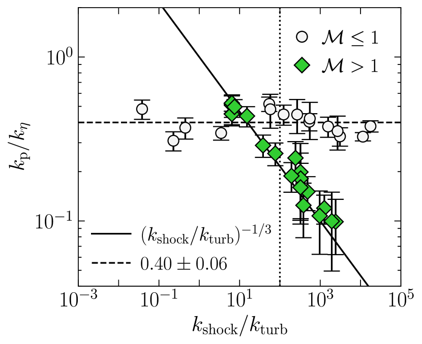
Figure 9: For each of our simulations we compare $k_{\mathrm{p}}/k_{\eta}$ with the reciprocal of our shock width model (Equation 26; note, formally, this is only valid for $\mathcal{M}>1$), where $\mathcal{M}\leq 1$ points are plotted as white circles, and $\mathcal{M}>1$ as green diamonds. We annotate the scaling relation $k_{\mathrm{p}}/k_{\eta}=(k_{\mathrm{shock}}/k_{\mathrm{turb}})^{-1/3}$ (relevant for compressible simulations) with a solid line, the average of the $\mathcal{M}\leq 1$ simulations $k_{\mathrm{p}}/k_{\eta}=0.40\pm 0.06$ (relevant for incompressible simulations) with a dashed line, and $k_{\mathrm{shock}}/k_{\mathrm{turb}}=10^{2}$ with a vertical dotted line, about which we see the supersonic points transition from the compressible to incompressible scaling.

In the inset axis of Figure 7 we test whether this shock width model can explain the difference between $k_{\mathrm{p}}$ and $k_{\eta}$ that we see (note that we colour points by the inverse shock width, so to emphasise that the numerator, $k_{\mathrm{shock}}$, is changing, and $k_{\mathrm{turb}}=2$ in the denominator is fixed). Here we plot the full set of $\mathcal{M}=5$ and $\mbox{Rm}=3000$ simulations; within this collection of runs, Re is varied via changing $\nu$ (i.e., $u_{\mathrm{turb}}$ and $k_{\mathrm{turb}}$ are fixed), and we find that the most turbulent simulation in this set, $\mathcal{M}$5Re3000Pm1, lies farthest from the $k_{\mathrm{p}}\sim k_{\eta}$ relation, while the most viscous simulation, $\mathcal{M}$5Re24Pm125, lies on the relation. Between these two limits, the inverse shock width (Equation 26) scales directly proportional to the deviation of each point from the $k_{\mathrm{p}}\sim k_{\eta}$ relation.

We demonstrate this more explicitly in Figure 9, which shows $k_{\mathrm{p}}/k_{\eta}$ as a function of $k_{\mathrm{shock}}/k_{\mathrm{turb}}$. It is clear that the majority of the $\mathcal{M}>1$ simulations (green diamond points) are well-fit by the empirical relationship

$$\frac{k_{\mathrm{p}}}{k_{\eta}}=\left(\frac{k_{\mathrm{shock}}}{k_{\mathrm{turb}}}\right)^{-1/3},$$ (27)

which we interpret to mean that shocks bring $k_{\mathrm{p}}$ from $k_{\eta}$ towards $k_{\mathrm{shock}}$, and the amount by which $k_{\mathrm{p}}$ shifts to larger scales is determined by the aspect ratio of typical shocks, i.e., ratio of the typical length compared with width of shocks in the medium. Since the forcing modes in all of our simulations are $k_{\mathrm{turb}}=2$, only $k_{\mathrm{shock}}$ changes with the properties of the medium (i.e., $\nu$) and flow (Re and $\mathcal{M}$), which is excellently captured by Equation 26. We hypothesise that the exponent $1/3$ in Equation 27 is likely associated with magnetic energy becoming concentrated into filamentary, shocked regions, which are inherently 1D structures embedded in 3D space.

In Figure 9 we see more evidence for a critical Reynolds number $\mbox{Re}_{\mathrm{crit}}\approx 100$ that separates $\mathcal{M}>1$ flows that support shocks ($\mbox{Re}>\mbox{Re}_{\mathrm{crit}}$) from those where strong viscosity prevents shocks from forming ($\mbox{Re}<\mbox{Re}_{\mathrm{crit}}$). In the high $\mathcal{M}$ limit $k_{\mathrm{shock}}/k_{\mathrm{turb}}=\mbox{Re}$, and thus $\mbox{Re}=\mbox{Re}_{\mathrm{crit}}\sim 100$ corresponds to $k_{\mathrm{shock}}/k_{\mathrm{turb}}\sim 100$; we highlight this value by the dotted vertical line in Figure 9. It is clear from the figure that this line roughly identifies where the $\mathcal{M}>1$ simulations transition from $k_{\mathrm{p}}/k_{\eta}\sim\mathrm{const}$ to $k_{\mathrm{p}}/k_{\eta}\sim(k_{\mathrm{shock}}/k_{\mathrm{turb}})^{-1/3}$. Indeed, one should notice that the seven red points that lie to the left of the vertical line in Figure 9 correspond with the seven that lie along the $k_{\mathrm{p}}\propto k_{\eta}$ relation in Figure 7, where in all seven cases $\mbox{Re}<100$.

We conclude that Figure 7 and Figure 9 can be explained simply by two distinct regimes. In the first, incompressible regime, the development of shocks is not supported by the properties of the plasma, whether it is because the velocity dispersion is too small ($\mathcal{M}\leq 1$) or because the viscosity is large enough to dissipate the supersonic velocities before shocks can form (i.e., $\mathcal{M}>1$ and $\mbox{Re}<\mbox{Re}_{\mathrm{crit}}$). This results in the well-known hierarchy of characteristic MHD scales where

$$\ell_{\mathrm{turb}}>\ell_{\nu}>\ell_{\eta}\sim\ell_{\mathrm{p}}.$$ (28)

In the compressible (shock-dominated; $\mathcal{M}>1$ and $\mbox{Re}>\mbox{Re}_{\mathrm{crit}}$) flow regime, however, shocks concentrate magnetic energy in large-scale, filamentary structures, which bring the peak magnetic field scale from the resistive scale to $\ell_{\mathrm{p}}\sim(\ell_{\mathrm{turb}}/\ell_{\mathrm{shock}})^{1/3}\ell_{\eta}\gg\ell_{\eta}$ (approaching $\ell_{\mathrm{p}}\sim\mbox{Re}^{1/3}\ell_{\eta}$ for $\mathcal{M}\gg 1$), so the hierarchy of scales becomes

$$\ell_{\mathrm{turb}}>\ell_{\mathrm{p}}>\ell_{\mathrm{shock}}>\ell_{\nu}>\ell_{\eta}.$$ (29)

Our characteristic shock width model, Equation 26, explains the growing proportion of large-scale magnetic energy in the magnetic energy distribution, and captures the transition between the compressible and incompressible flow regimes during the kinematic phase of a supersonic SSD. Moreover, we find that the scaling in both flow regimes remains consistent with our simulations, even in the asymptotic, high-Rm plasma regime, as evidenced by our two highest, $\mbox{Rm}=10^{4}$ simulations in both the incompressible and compressible regimes (namely $\mathcal{M}$0.3Re2000Pm5 and $\mathcal{M}$5Re2000Pm5) agreeing with the Equation 28 and 29 scalings, respectively.

In the next section, we show that shocks not only concentrate magnetic energy into larger-scale coherent structures (as demonstrated here), but they also change the underlying magnetic field geometry.

3.7 Magnetic Field Curvature

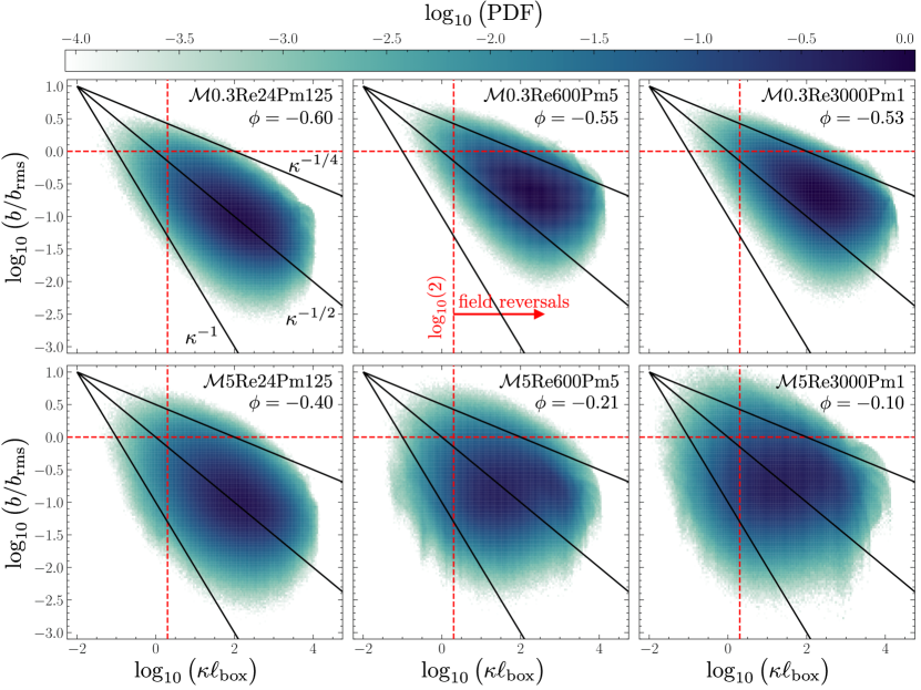
Figure 10: Joint distributions of the relative magnetic field strength, $b/b_{\mathrm{rms}}$, and the magnetic field-line curvature, $\kappa$ (measured in units of inverse $\ell_{\mathrm{box}}$), for the same six simulations as in Figure 2. In all panels we report the Pearson correlation coefficient $\phi$ (given by Equation 31) between $\log_{10}(b/b_{\mathrm{rms}})$ and $\log_{10}(\kappa/\kappa_{\mathrm{rms}})$. We also annotate a $b\sim\kappa^{-1/2}$ scaling, which is associated with a curvature relation where the magnetic tension is exactly balanced by the turbulent stretching (the symmetric rate of shear component in $\nabla\otimes\mathrm{{\mn@boldsymbol{\mathit{v}}}}$; Schekochihin et al. 2001, 2004); see Section 3.7 for a discussion. We also show $b\sim\kappa^{-1/4}$ and $b\sim\kappa^{-1}$ to guide the eye. The red, horizontal, dashed lines indicates $b=b_{\mathrm{rms}}$, while the red, vertical, dashed lines indicate $\kappa\ell_{\mathrm{box}}=2$, which marks the transition between fields that can ($\kappa\ell_{\mathrm{box}}\geq 2$) and cannot ($\kappa\ell_{\mathrm{box}}<2$) reverse within the box-domain. The $b\sim\kappa^{-1/2}$ scaling holds well (on average) for the subsonic cases (top row), but breaks down for the supersonic cases (bottom two right panels), which is most likely due to the presence of shocks being able to compress and grow the field without necessarily modifying the curvature.

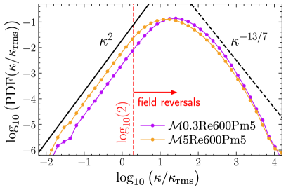
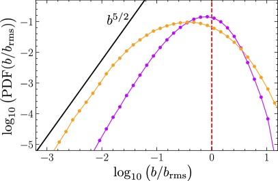
Figure 11: Probability density functions (PDFs) of the magnetic field-line curvature, $\kappa$ (measured in units of box-length; left panel), and the normalised magnetic field amplitude (right panel), $b/b_{\mathrm{rms}}$, for $\mathcal{M}$0.3Re600Pm5 and $\mathcal{M}$5Re600Pm5. We annotate $\kappa^{2}$ and $\kappa^{-13/7}$ in the left panel, and $b^{5/2}$ in the right panel, where $\kappa^{-13/7}$ is a theoretical prediction for the $\kappa$ distribution for magnetic fields in the kinematic phase of a subsonic turbulent dynamo (Schekochihin et al., 2002c). We find only a negligible difference between $p(\kappa\ell_{\mathrm{box}})$ for the $\mathcal{M}<1$ (purple) and $\mathcal{M}>1$ (yellow) simulations, but there is significantly more low and high $b/b_{\mathrm{rms}}$ probability densities in the $\mathcal{M}>1$ simulation. Hence we conclude that the weakening correlation between $\kappa$ and $b$ (shown in Figure 10) is caused from shock compressions that grow and shrink $b$ without influencing $\kappa$.

While we have shown that shocks are responsible for reorganising magnetic energy into large-scale, filamentary structures, here we will show that in doing so, they also completely change the underlying magnetic field geometry. To quantify field geometry we compute the curvature of magnetic field lines

$$\kappa=\left\|\left(\widehat{\mathrm{{\mn@boldsymbol{\mathit{b}}}}}\cdot\nabla\right)\widehat{\mathrm{{\mn@boldsymbol{\mathit{b}}}}}\right\|,$$ (30)

at every point in a simulation domain, where $\widehat{\mathrm{{\mn@boldsymbol{\mathit{b}}}}}=\mathrm{{\mn@boldsymbol{\mathit{b}}}}/|\mathrm{{\mn@boldsymbol{\mathit{b}}}}|$ is the tangent vector to the field, and curvature points in the $\widehat{\mathrm{{\mn@boldsymbol{\mathit{\kappa}}}}}=(\widehat{\mathrm{{\mn@boldsymbol{\mathit{b}}}}}\cdot\nabla)\widehat{\mathrm{{\mn@boldsymbol{\mathit{b}}}}}/\kappa$ direction. The radius of curvature of the field in units of box length is then $\ell_{\mathrm{box}}/\kappa$.

In Figure 10 we plot the time-averaged, joint distributions of the relative magnetic field strength, $b/b_{\mathrm{rms}}$ (normalising out the dynamo growth in $b$), and field-line curvature, $\kappa\ell_{\mathrm{box}}$, for the same six simulations as in Figure 2, namely $\mathcal{M}$0.3Re24Pm125, $\mathcal{M}$0.3Re600Pm5, and $\mathcal{M}$0.3Re3000Pm1 in the top row, and $\mathcal{M}$5Re24Pm125, $\mathcal{M}$5Re600Pm5, and $\mathcal{M}$5Re3000Pm1 in the bottom row, respectively. Focusing first only on the three subsonic simulations (top row of Figure 10), we find that the $(\kappa,b)$ distributions in both the viscous (left panel) and turbulent SSDs (middle and right panels) appear to have the same overall shape, where the weakest magnetic fields have the largest curvature, e.g., have the most field reversals, and conversely the strongest fields are the straightest. Here we find evidence of a scaling consistent with $b\sim\kappa^{-1/2}$, which was first demonstrated by Schekochihin et al. (2004) (as opposed to $b\sim\kappa^{-1}$ as previously suggested by Schekochihin et al. 2002c and Brandenburg et al. 1995) for incompressible SSDs and more recently by Kempski et al. (2023) using $\mathcal{M}<1$ SSD and weak mean-field simulations to study cosmic ray propagation. Schekochihin et al. (2004) associates the $b\sim\kappa^{-1/2}$ anti-correlation with a “folded field” geometry, where the shearing (tearing) velocity gradient tensor and the magnetic tension are balanced.

In contrast, the supersonic SSDs (bottom row of Figure 10), show a significantly weaker relationship between the field strength and field-line curvature, with the relative statistical independence of $b$ and $\kappa$ increasing as we move from the most viscous flow (bottom left) to the most turbulent (bottom right). In the turbulent, supersonic regime, it is clear that both strong ($b>b_{\mathrm{rms}}$) and weak ($b<b_{\mathrm{rms}}$) field lines can maintain a straight configuration ($\kappa\ell_{\mathrm{box}}<2$), although we still see a dearth of high curvature ($\kappa\ell_{\mathrm{box}}>2$) for strong magnetic fields ($b>b_{\mathrm{rms}}$; i.e., the upper right quadrant of the plot is empty). We quantify this growing independence between $b$ and $\kappa$ for each of our simulations in Figure 10 by computing the Pearson correlation coefficient between $\log_{10}(b/b_{\mathrm{rms}})$ and $\log_{10}(\kappa)$,

$$\phi=\frac{\mathrm{cov}\big{[}\log_{10}(b/b_{\mathrm{rms}})\log_{10}(\kappa\ell_{\mathrm{box}})\big{]}}{\sqrt{\mathrm{var}\big{[}\log_{10}(b/b_{\mathrm{rms}})\big{]}\,\mathrm{var}\big{[}\log_{10}(\kappa\ell_{\mathrm{box}})\big{]}}},$$ (31)

where $\mathrm{cov}[\ldots]$ and $\mathrm{var}[\ldots]$ are the covariance and variance operators, respectively. We annotate these values in each panel of Figure 10.

The numerical results confirm our qualitative, visual impression: $b$ and $\kappa$ are strongly anti-correlated (and in the $\log$-$\log$ domain, this translates to being linearly anti-correlated, as one expects for the Schekochihin et al. 2004-type models) in both the subsonic, viscous flow regime (upper left panel, $\phi=-0.60$) and subsonic, turbulent flow regimes (upper middle and right panels; $\phi=-0.55$ and $\phi=-0.53$, respectively). The anti-correlation remains, but becomes weaker for supersonic flows that are too viscous to support shocks (lower left panel, $\phi=-0.40$), and then the anti-correlation almost completely disappears once strong shocks enter the picture (lower middle and right panels; $\phi=-0.21$ and $\phi=-0.10$, respectively).

However, we find that what drives the anti-correlation in Figure 10 is not the distribution of $\log_{10}(\kappa)$, but the distribution of $\log_{10}(b)$. We demonstrate this in Figure 11, where we plot the time-averaged (over the kinematic phase) PDF of $\log_{10}(\kappa)$ (left panel) and $\log_{10}(b)$ (right panel) for our two representative simulations (again, $\mathcal{M}$0.3Re600Pm5 and $\mathcal{M}$0.3Re600Pm5). Notice that while the $\log_{10}(\kappa)$ distributions look very similar, the $\log_{10}(b)$ distribution changes significantly between the two flow regimes, with the magnetic amplitude distribution becoming much broader (a greater proportion of the fields are weaker or stronger than $b_{\mathrm{rms}}$) in the supersonic compared with the subsonic SSD. This is likely due to shocks growing magnetic energy via compression and flux-freezing, which do not change the structure of the magnetic field significantly. There is a marginal increase in straighter fields, in the compressible regime, however for $\mathcal{M}<10$ this effect is largely negligible.

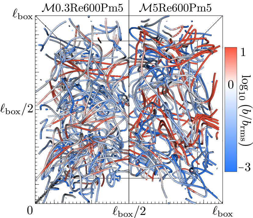
Figure 12: Magnetic field streamlines for $\mathcal{M}$0.3Re600Pm5 and $\mathcal{M}$5Re600Pm5 plotted on the left- and right-side half of the cube, respectively, for a time realisation midway through each simulation’s kinematic phase. The streamlines are coloured based on the normalised magnetic field magnitude, $b/b_{\mathrm{rms}}$, using a colour-range that spans across the same range of $b/b_{\mathrm{rms}}$ as plotted in the right panel of Figure 11.

This picture is supported by Figure 12, where we plot $100$ magnetic field streamlines for our two representative simulations at a time realisation midway through the kinematic phase. $\mathcal{M}$0.3Re600Pm5 is plotted on the left half of the cube, and $\mathcal{M}$5Re600Pm5 is plotted on the right half. The key takeaway is, in line with our findings above, that while magnetic field lines in both regimes thread the simulation domain with an equally “chaotic structure” (the field-line curvature distribution remains largely unchanged), the magnitude of the field corresponding with different field-line structures is different in the incompressible and compressible regimes. In $\mathcal{M}$0.3Re600Pm5, all straight field lines are strong ($b>b_{\mathrm{rms}}$; red), and all field lines with intense curvature are weak ($b<b_{\mathrm{rms}}$; blue). In contrast, for $\mathcal{M}$5Re600Pm5 some curved fields are strong and others are weak, and likewise, straight fields can also be strong or weak, although there are slightly more straight fields that are strong (compare the two right hand quadrants in the middle panel on the bottom row of Figure 10).

Overall, our quantitative analysis of the field geometry supports our interpretation and Schekochihin et al. (2004, 2002b)’s models of the relationship between the magnetic peak energy scale and resistive dissipation scale in the previous section: in the incompressible flow regime (where shocks are absent), the SSD in the kinematic phase produces a “folded-field” geometry where magnetic energy becomes concentrated at $k_{\eta}$ – the smallest scales possible (a state that Schekochihin et al. (2004) shows persists into the saturated phase), and $b\sim\kappa^{-1/2}$, but in the compressible flow regime (where shocks are ubiquitous), this organisation of the field geometry disappears. Again, we emphasise that the distribution of magnetic field-line curvature remains essentially the same, regardless of the flow regime, but curvature in the compressible regime no longer correlates with magnetic-field strength.

4 Discussion

Our findings in this study are relevant to a wide range of astrophysical systems, but here we highlight galaxy mergers and cosmic ray (CR) propagation as two particularly interesting cases, since the former case creates an environment that stimulates a kinematic phase SSD, while the latter has recently been explored in terms of underlying curvature statistics of the magnetic field. We highlight how it is of key importance to differentiate between the incompressible and compressible SSD regimes (see the end of Section 3.6 for our distinction between these two regimes) for these astrophysical processes.

4.1 Galaxy Mergers

Recent studies (e.g.,  Pakmor et al., 2014, 2017; Brzycki & ZuHone, 2019; Whittingham et al., 2021, 2023; Pfrommer et al., 2022) have highlighted the important role that turbulent SSD amplified magnetic fields play in shaping the overall size and shape of galaxy merger remnants, particularly those involving gas-rich disc galaxies. These merger events are transformative for the galactic gas dynamics, with strong magnetic fields modifying the transport of angular momentum, and aiding in pressure support against collapse (Whittingham et al., 2021). Collectively, these factors contribute to the formation of remnant galaxies with prominent spiral arms, which are notably missing in the smaller scale, compact remnants produced by merger simulations that do not include the effects of magnetic fields (e.g.,  Whittingham et al., 2021, 2023).

An important and as-yet unexplained property of the amplified magnetic fields is that the magnetic energy peaks on $\ell_{\mathrm{p}}\gtrsim\mbox{kpc}$ scales during the kinematic phase of the SSD produced by the merger (e.g.,  Rodenbeck & Schleicher, 2016; Basu et al., 2017; Brzycki & ZuHone, 2019; Whittingham et al., 2021), in stark contrast to the significantly smaller-scale fields predicted by incompressible SSD theory. For example, Whittingham et al. (2021) simulate a galaxy merger using ideal MHD (i.e., no explicit viscosity or resistivity), so their simulations have $\ell_{\eta}\sim\ell_{\nu}\sim\ell_{\mathrm{res}}$, where $\ell_{\mathrm{res}}$ is the numerical resolution. This is non-uniform in their moving-mesh arepo simulations, but as a rough estimate we note that in the $\sim 5\,\mbox{kpc}$ region where they observe most of the dynamo amplification, they report a mean density $\sim 10^{7}$ $M_{\odot}$ kpc^-3, which given their baryonic resolution $m_{\rm b}\sim 10^{4}M_{\odot}$ and characteristic Mach number $\mathcal{M}\sim 3$, corresponds with $\ell_{\mathrm{res}}\sim 100\,\mbox{pc}$, and $\mbox{Re}\sim 1000$, though the latter may be a slight underestimate since presumably their resolution is finest in regions of strong dissipation. Regardless, if an incompressible SSD were responsible for setting $\ell_{\mathrm{p}}$, then one would expect $\ell_{\mathrm{p}}\sim\ell_{\eta}\sim 100\,\mbox{pc}$, which is significantly smaller than the $\ell_{\mathrm{p}}\gtrsim 1\,\mbox{kpc}$ they find.

This discrepancy is resolved if we notice that mergers not only induce compressions, but also drive supersonic turbulent velocity fields (Geng et al., 2012; Sparre et al., 2022). For example, Sparre et al. (2022) find that the gas bridge connecting merging galaxies is dominated by $1.6\leq\mathcal{M}\leq 3.3$ turbulence on $\ell_{\mathrm{turb}}\lesssim 10\,\mbox{kpc}$ scales. Magnetic amplification in these galaxy mergers should therefore be attributed to a compressible rather than an incompressible SSD, which we showed in Section 3.6 brings magnetic energy to larger scales by a factor $\sim(\ell_{\mathrm{turb}}/\ell_{\mathrm{shock}})^{1/3}\gtrsim 10$. This would naturally explain why they see magnetic fields structured on $\sim\mbox{kpc}$ scales, much larger than the magnetic dissipation scales in their simulations.

It is important to note that, while the discrepancy between the value of $\ell_{\mathrm{p}}$ produced during galaxy mergers and that predicted by subsonic SSD models is only a factor of $\sim 10-100$ in the context of simulations, the discrepancy is much larger in reality, where dissipation scales are much smaller than can be achieved in simulations. Incompressible SSDs predict (e.g., Schekochihin et al. 2004; Fundamental Scales I; Brandenburg et al. 2023; see also Section 3.6) $\ell_{\mathrm{p}}\sim\ell_{\eta}\sim\ell_{\nu}\mbox{Pm}^{-1/2}\sim\ell_{\mathrm{turb}}\mbox{Re}^{-3/4}\mbox{Pm}^{-1/2}\sim\ell_{\mathrm{turb}}\mbox{Re}^{-1/4}\mbox{Rm}^{-1/2}$. Assuming typical plasma parameters for the warm ionised phase of the ISM (Rincon, 2019; Ferrière, 2019; Shukurov & Subramanian, 2021; Brandenburg & Ntormousi, 2023), $\mbox{Re}\sim 10^{7}$ and $\mbox{Rm}\sim 10^{18}$, an incompressible SSD is therefore expected to produce magnetic fields that are peaked $\sim 10$ orders of magnitude smaller than the turbulent scale; for a $\sim 10\,\mbox{kpc}$-scale galaxy merger, this would correspond to $\sim 10^{-2}\,\mbox{AU}$! There is clearly a huge discrepancy between this prediction and $\ell_{\mathrm{p}}\gtrsim\mbox{kpc}$ observed magnetic fields, which are structured on much larger scales. This highlights that compressible SSD amplification, which organises magnetic fields on much larger scales than incompressible SSDs, is a much more plausible explanation for the magnetic structure produced during galaxy mergers.

4.2 Cosmic ray Propagation

Butsky et al. (2023) has recently suggested that intermittent magnetic field fluctuations are necessary for regulating low-energy ($\sim{\rm MeV}$ – ${\rm TeV}$) cosmic ray (CR) scattering in the Milky Way. Kempski et al. (2023) and Lemoine (2023) provide a potential source of magnetic field intermittency: intense regions of curved magnetic fields that reverse upon themselves, i.e., magnetic field reversals. They argue that if magnetic fields are dominated by their fluctuating field ($\delta b/b_{0}\gg 1$; as is the case for our simulations because there is no $\mathrm{{\mn@boldsymbol{\mathit{b}}}}_{0}$) then there is an energy dependent diffusion process associated with CR particles scattering off of magnetic fields due to the field’s reversal being on scales that are resonant with the gyroradius of the CR.

The Kempski et al. (2023) model contains a resonance criterion derived from the assumption that $b\sim\kappa^{1/2}$, which we have shown holds in incompressible plasma regimes, but breaks down in supersonic turbulence. Instead, Section 3.7 shows that magnetic field strength and curvature tend towards independence in the supersonic turbulent regime. That is not to say that the magnetic field does not also support reversals in the supersonic regime; in probability density, it has just as many as the subsonic regime (see Figure 11). However the magnetic field amplitude is no longer constrained to a curvature relation, and hence the gyroradii of the CRs are free to vary independently of the curvature. Therefore these models will need to be modified for the $\mathcal{M}>1$ turbulent regime, where parts of the volume will have no resonances.

The turbulent, $\mathcal{M}>1$ regime is important because (1) most of the gas volume of the Milky Way is filled by hot and warm ionized phases, where flows are sub- to transsonic, $\mathcal{M}\lesssim 2$ (e.g.,  Gaensler et al., 2011; Draine, 2011; Shukurov & Subramanian, 2021; Beattie et al., 2022a), hence shocks may form even in the volume-filling phases of the ISM, and (2) by mass – and thus if one is interested in the majority of the targets for $\gamma$-ray production, for example – the Milky Way is dominated by cold and warm neutral phases within which flows are supersonic, $\mathcal{M}\gtrsim 4-10$ (e.g.,  Federrath et al., 2016; Beattie et al., 2019; Nguyen et al., 2019). Hence, one cannot ignore the difference between incompressible and compressible curvature statistics for CR propagation models.

5 Summary & Conclusions

In this study we explore how both the energy spectrum (see Section 3.6) and field-line curvature (see Section 3.7) of magnetic fields produced during the exponential-growing (kinematic) phase of small-scale dynamos (SSDs) depend upon the plasma flow regime (from subsonic $\mathcal{M}<1$ to supersonic $\mathcal{M}>1$, and viscous $\mbox{Re}<\mbox{Re}_{\mathrm{crit}}\approx 100$ to turbulent $\mbox{Re}>\mbox{Re}_{\mathrm{crit}}$ flows). To do so, we have used direct numerical simulations where we explicitly control the velocity field magnitude, as well as the dissipation rates of kinetic and magnetic energy to explore a wide range of $\mathcal{M}$, hydrodynamic Reynolds number Re, and magnetic Prandtl number Pm. This has allowed us to extend our understanding of SSD-amplified magnetic fields into the previously poorly-understood regime of supersonic SSDs. In particular, we have identified new relationships between the important characteristic length scales in a SSD – the outer scale of turbulence $\ell_{\mathrm{turb}}$, the kinetic energy dissipation scale $\ell_{\nu}$, the magnetic energy dissipation scale $\ell_{\eta}$, and the peak magnetic energy scale $\ell_{\mathrm{p}}$ – as a function of the fundamental plasma numbers: $\mathcal{M}$, Re, and Pm. We complement this with a study of the statistics of magnetic field-line curvature, which support our findings.

We list our key results below:

• During the kinematic phase of SSDs the kinetic energy dissipation scale $\ell_{\nu}$ varies with Re and $\mathcal{M}$ as expected for hydrodynamic flows (see the left panel in Figure 6). That is, we find three regimes: $\ell_{\nu}\sim\ell_{\mathrm{turb}}\,\mbox{Re}^{3/4}$ for $\mathcal{M}\leq 1$ flows where $\mbox{Re}>\mbox{Re}_{\mathrm{crit}}$ (turbulent subsonic flows), which corresponds to Kolmogorov (1941)-like scaling, $\ell_{\nu}\sim\ell_{\mathrm{turb}}\,\mbox{Re}^{2/3}$ for $\mathcal{M}>1$ (supersonic) flows, which corresponds to Burgers (1948)-like scaling, and finally $\ell_{\nu}\sim\ell_{\mathrm{turb}}\,\mbox{Re}^{3/8}$ for $\mathcal{M}\leq 1$ and $\mbox{Re}<\mbox{Re}_{\mathrm{crit}}$ (subsonic viscous) flows (first shown in Fundamental Scales I), which has a scaling intermediate between the Kolmogorov (1941) and Burgers (1948) cases.
  

• The magnetic dissipation scale $\ell_{\eta}$ is related to the kinetic dissipation scale as $\ell_{\eta}\sim\ell_{\nu}\,\mbox{Pm}^{1/2}$, regardless of the plasma flow regime. Since this scaling relation, first proposed by Schekochihin et al. (2002b), follows from assuming that $\ell_{\eta}$ is located on the scale where the viscous eddy shearing rate is balanced by Ohmic dissipation, we conclude that the viscous (smallest-scale) kinetic eddies are always the most efficient at amplifying magnetic energy during the kinematic phase of $\mbox{Pm}\geq 1$ SSDs, invariant to the underlying properties of the kinetic motion, as long as the motions are isotropic.
  

• The magnetic peak scale $\ell_{\mathrm{p}}$ and the associated statistics of the magnetic field-line curvature $\kappa$ produced by SSDs are very different for incompressible (i.e., either $\mathcal{M}\leq 1$, or $\mathcal{M}>1$ and $\mbox{Re}<\mbox{Re}_{\mathrm{crit}}$) and compressible (i.e., $\mathcal{M}>1$ and $\mbox{Re}>\mbox{Re}_{\mathrm{crit}}$) flows. The incompressible case behaves as predicted by the “folded field” model of Schekochihin et al. (2002b, 2004), where the field-line curvature $\kappa$ and the field magnitude $b$ are strongly anti-correlated (see Figure 10) as $b\sim\kappa^{-1/2}$, and the magnetic energy becomes concentrated on the smallest scales allowed by magnetic dissipation, which results in the hierarchy of characteristic length scales $\ell_{\mathrm{turb}}>\ell_{\nu}>\ell_{\eta}\sim\ell_{\mathrm{p}}$. By contrast in the compressible regime supersonic turbulence naturally gives rise to shocks with characteristic shock width $\ell_{\mathrm{shock}}\sim\mathcal{M}^{2}\ell_{\mathrm{turb}}/[\mbox{Re}\,(\mathcal{M}-1)^{2}]$, which we derive in Section 3.6. These shocks grow magnetic energy via flux-freezing and compression, which changes the distribution of $b$ amplitudes, essentially destroying the anti-correlation between $b$ and $\kappa$, but notably, does not change the distribution of field-line curvature. As $\mathcal{M}\to\infty$, the two magnetic field-line quantities tend towards independence, $b\sim\kappa^{0}$. Moreover, these shocks also concentrate magnetic fields on a scale $\ell_{\mathrm{p}}\sim(\ell_{\mathrm{turb}}/\ell_{\mathrm{shock}})^{1/3}\ell_{\eta}\gg\ell_{\eta}$; in the high $\mathcal{M}$ limit, this produces $\ell_{\mathrm{p}}\sim\mbox{Re}^{1/3}\ell_{\eta}$, giving rise to a hierarchy $\ell_{\mathrm{turb}}>\ell_{\mathrm{p}}>\ell_{\mathrm{shock}}>\ell_{\nu}>\ell_{\eta}$, where magnetic energy becomes concentrated on scales much larger than the magnetic dissipation scale.
  

• We discuss a longstanding problem about the generation of large-scale magnetic fields in the context of galaxy mergers (but potentially can be more broadly applied to other young galaxies, such as the recent observation of a young starburst galaxy with a large-scale field in Geach et al. 2023). We argue that through supersonic turbulence – a natural state for these galaxies, since both early galaxies and galaxy mergers feature dense gas that cools quickly, rendering their flows supersonic – the compressible SSD can construct fields whose size scale can, for sufficiently large Re, approach the outer scale of the turbulence, in complete contrast with fields produced by the incompressible SSD, which are concentrated at much smaller resistive scales $\ell_{\mathrm{p}}\sim\ell_{\eta}$.
  

• We also discuss the implications our results have on models of cosmic ray scattering based on resonances between the size-scale of magnetic field reversals and the gyro-radius of the cosmic ray, (e.g., Kempski et al., 2023). We suggest that for supersonic plasmas, which may be a significant portion of the interstellar medium of the Milky Way, these resonances may not work, since the magnetic field amplitude ($\sim$ gyro-radius) and underlying field curvature become independent from one another.

Data Availability

The dataset underlying Table 1 and Table 2 is publicly available from MNRAS. Access to data beyond this will be shared upon reasonable request to the corresponding author.

Appendix A Density-Weighted Hydrodynamic Reynolds Number

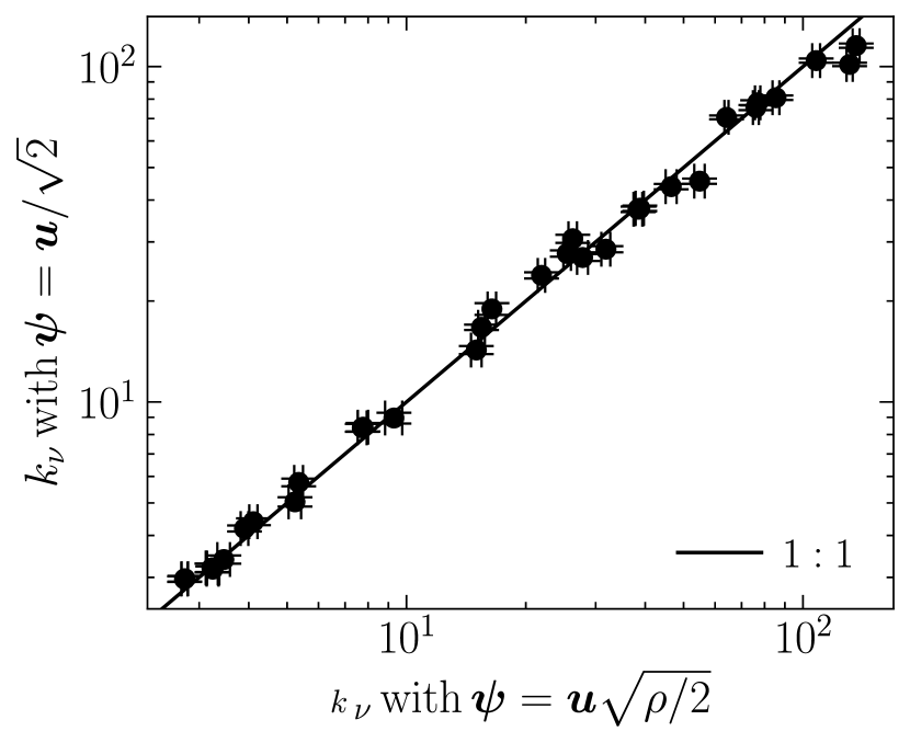
Figure 13: For each simulation setup in Table 1, we compare the converged (see Section 3.4 for details) characteristic viscous wavenumber, $k_{\nu}$, measured from Equation 16 constructed with $\mathrm{{\mn@boldsymbol{\mathit{\psi}}}}=\mathrm{{\mn@boldsymbol{\mathit{u}}}}/\sqrt{2}$ (y-axis; studied in the main text), and $k_{\nu}$ constructed with $\mathrm{{\mn@boldsymbol{\mathit{\psi}}}}=\mathrm{{\mn@boldsymbol{\mathit{u}}}}\sqrt{\rho/2}$ (x-axis).

In the main text (see Section 3.3.1) we measured characteristic viscous wavenumbers, $k_{\nu}$, from kinetic energy spectra, $E_{\mathrm{kin}}(k)$, constructed only from the velocity field (that is, $\mathrm{{\mn@boldsymbol{\mathit{\psi}}}}=\mathrm{{\mn@boldsymbol{\mathit{u}}}}/\sqrt{2}$ in Equation 13). An alternative, popular definition for compressible flows (see for example Federrath et al., 2010; Federrath, 2013; Schmidt & Grete, 2019; Grete et al., 2021, 2023), which accounts for density fluctuations, is $E_{\mathrm{kin}}(k)$ constructed from Equation 13 with $\mathrm{{\mn@boldsymbol{\mathit{\psi}}}}=\mathrm{{\mn@boldsymbol{\mathit{u}}}}\sqrt{\rho/2}$. This definition is based on the idea that $E_{\mathrm{kin}}$ should have units of kinetic energy, and such that $\psi^{2}$ needs to be a positive definite quantity (Kida & Orszag, 1990).

In Figure 13 we compare converged (with numerical resolution; see Section 3.4) $k_{\nu}$ measured from both definitions for $E_{\mathrm{kin}}(k)$, for all our simulations, plotting $k_{\nu}$ derived from the $\mathrm{{\mn@boldsymbol{\mathit{\psi}}}}=\mathrm{{\mn@boldsymbol{\mathit{u}}}}\sqrt{\rho/2}$ spectrum on the x-axis, and $\mathrm{{\mn@boldsymbol{\mathit{\psi}}}}=\mathrm{{\mn@boldsymbol{\mathit{u}}}}/\sqrt{2}$ on the y-axis. We show that $k_{\nu}$ measured from the different definitions for $E_{\mathrm{kin}}(k)$ scales 1:1, and therefore our measurements for $k_{\nu}$ in the kinematic phase of the SSD are robust and insensitive to density fluctuations.

Appendix B Resistive Scales Measured from Magnetic Reynolds Spectra

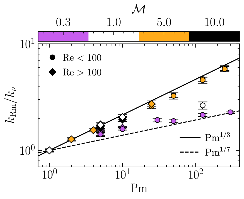
Figure 14: For each simulation in Table 1, we plot the separation between the wavenumber where magnetic Reynolds number is one, $k_{\rm Rm}:\mbox{Rm}(k)=1$, and the viscous wavenumber, $k_{\nu}$ (using the definition in the main text, see Section 3.3.1), via $k_{\rm Rm}/k_{\nu}$ and compare this separation with the magnetic Prandtl number. We plot simulations with $\mbox{Re}<\mbox{Re}_{\mathrm{crit}}\approx 100$ as circles, and $\mbox{Re}>\mbox{Re}_{\mathrm{crit}}$ as diamonds, and colour points by the sonic Mach number. We also annotate two power laws $\mbox{Pm}^{1/3}$ (solid line) and $\mbox{Pm}^{1/7}$ (dashed line) to highlight the different empirical scaling of $k_{\rm Rm}/k_{\nu}$ for subsonic and supersonic SSDs.

Given the success of our definition for the viscous scale (Equation 16), one may be tempted to define the resistive scale analogously. That is

$$k_{\rm Rm}(t)=\texttt{argmin}_{k}\Big{[}\mathcal{I}\Big{\{}\Big{|}\mbox{Rm}(k,t)-1\Big{|}\Big{\}}\Big{]},$$ (32)

where $\mbox{Rm}(k,t)\equiv u_{\mathrm{turb}}(k,t)/\eta k$. However, in Figure 14 we show that this wavenumber, $k_{\rm Rm}$, does not correspond with $k_{\eta}$ derived from Equation 17. In this figure we plot the separation between the converged (with numerical resolution; see Section 3.4), time averaged (over the kinematic phase) $k_{\rm Rm}$ and $k_{\nu}$, for each of our simulations in Table 1, and show that this separation does not scale like $\mbox{Pm}^{1/2}$, which we showed in Figure 6 is the case irrespective of the flow regime.

We interpret this to mean that, whilst a unit analysis of the magnetic Reynolds number gives $\mbox{Rm}\sim u_{\mathrm{turb}}\ell_{\mathrm{turb}}/\eta$, more directly, Rm (Equation 9) controls the relative importance of the induction term, $\nabla\times(\mathrm{{\mn@boldsymbol{\mathit{u}}}}\times\mathrm{{\mn@boldsymbol{\mathit{b}}}})$, compared with magnetic dissipation, $\eta\nabla\times\mathrm{{\mn@boldsymbol{\mathit{j}}}}$. However, each of these terms operate on different characteristic scales, (scales associated with $\ell_{\nu}$ for the induction, as we showed in Figure 6, and scales associated with $\ell_{\eta}$ for the dissipation). These details are not captured by only considering the influence of $u_{\mathrm{turb}}\ell_{\mathrm{turb}}/\eta$, i.e., only considering the velocity structures for building the scale dependence (as we did with Equation 14). In fact, we know from Section 3.5 that $k_{\eta}$ should be largely independent of the kinetic cascade statistics, which Equation 32 is completely dependent upon (along with the material properties of the magnetic field).

Appendix C Magnetic correlation scale

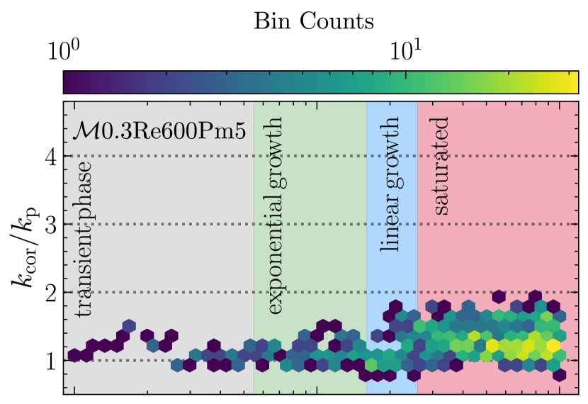
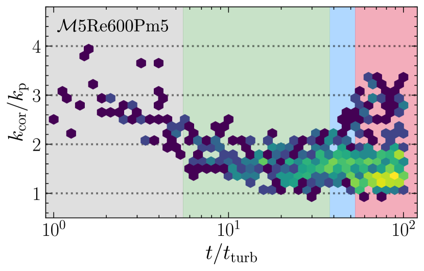
Figure 15: Time evolution of the magnetic correlation scale, $k_{\mathrm{cor}}$ (from Equation 33), compared with the magnetic peak scale, $k_{\mathrm{p}}$ (from Equation 18), for $\mathcal{M}$0.3Re600Pm5 and $\mathcal{M}$5Re600Pm5 in the top and bottom panels, respectively. We highlight the transient phase of the simulation in grey, followed by the exponential growth (kinematic), linear growth, and saturated SSD phases in green, blue, and red, respectively.

Schekochihin et al. (2004) and Galishnikova et al. (2022) assume that the magnetic correlation (coherence) wavenumber,

$$k_{\mathrm{cor}}(t) =\int_{0}^{\infty}E_{\mathrm{mag}}(k,t)\,\mathrm{d}k\Big{/}\int_{0}^{\infty}k^{-1}E_{\mathrm{mag}}(k,t)\,\mathrm{d}k,$$ (33)

is proportional to the magnetic peak wavenumber, $k_{\mathrm{p}}$, which Beattie et al. (2023) showed seemed to be qualitatively true not only in the kinematic phase, but also in the saturated phase. It is not clear whether this assumption would be valid for supersonic SSD amplified fields, where the magnetic energy spectrum is broadened by shocks when $\mathcal{M}>1$ (see the bottom panel in Figure 4). To test this, we compute $k_{\mathrm{cor}}$ and $k_{\mathrm{p}}$ for our two representative simulations, $\mathcal{M}$0.3Re600Pm5 and $\mathcal{M}$5Re600Pm5 at $N_{\mathrm{res}}^{3}=576^{3}$. In Figure 15 we compare the time evolution of these two scales by plotting $k_{\mathrm{cor}}/k_{\mathrm{p}}$ computed throughout the simulation for both setups. We colour individual hexagon-bins based on the number of occurrences, and shade the time range corresponding with the transient, exponential growth (kinematic), linear growth, and saturated phases grey, green, blue, and red, respectively.

As expected for $\mathcal{M}$0.3Re600Pm5, we find evidence that during the kinematic phase $k_{\mathrm{cor}}\sim k_{\mathrm{p}}$, but this relationship appears to weaken into the saturated state. For $\mathcal{M}$5Re600Pm5 we find that $k_{\mathrm{cor}}>k_{\mathrm{p}}$ at all times. Initially $k_{\mathrm{cor}}\gg k_{\mathrm{p}}$, but gradually as the magnetic field becomes strong enough to suppress deformation on the smallest scales, $k_{\mathrm{cor}}/k_{\mathrm{p}}$ tends toward $\gtrsim 1$. Here $k_{\mathrm{cor}}>k_{\mathrm{p}}$ arises due to the magnetic energy distribution becoming broader due to shocks compressing magnetic energy into long, thin (i.e., filamentary) structures, with the typical length of these shocked regions adding energy on low-k modes, and the typical width (see our model Equation 26) adding energy to the spectrum on high-k modes.

Appendix D Fit Parameters Derived from Measuring Scale Convergence

In Section 3.4 we highlighted numerical convergence for two of our representative simulations, namely $\mathcal{M}$0.3Re600Pm5 and $\mathcal{M}$5Re600Pm5. We also performed the same convergence study for all of our other simulation setups in Table 1, so here, for each of our simulation setups, we list the two fitted parameters: (1) critical numerical resolution, $N_{\mathrm{res},\mathrm{crit}}$, required for wavenumber convergence, and (2) the rate of convergence, $R$, for the viscous (column 2), resistive (column 3), and magnetic peak wavenumbers (column 4).

For all of our viscous flow simulations, where $\mbox{Re}\leq\mbox{Re}_{\mathrm{crit}}\approx 100$, we find that our measurement for $k_{\nu}$ (and $k_{\mathrm{p}}$ in the case of $\mathcal{M}$5Re10Pm25) converged at even our lowest resolution runs (i.e., as expected, we do not need much resolution to resolve low-Re dynamics). In these cases, we report the lowest resolution run we performed as $N_{\mathrm{res},\mathrm{crit}}$, and report no value for $R$, in Table 2.

Table 2: Convergence properties of characteristic MHD wavenumbers.

Sim. ID	$k_{\nu}$			$k_{\eta}$			$k_{\mathrm{p}}$
	$N_{\rm res,crit}$	$R$		$N_{\rm res,crit}$	$R$		$N_{\rm res,crit}$	$R$
(1)	(2)			(3)			(4)
$\mathcal{M}=0.3$
$\mathcal{M}$0.3Re500Pm1	$34.7\pm 1.9$	$0.8\pm 0.1$		$67.8\pm 8.7$	$1.0\pm 0.2$		$31.6\pm 13.4$	$0.9\pm 0.8$
$\mathcal{M}$0.3Re100Pm5	$18.0$	–		$54.4\pm 10.4$	$1.0\pm 0.2$		$31.4\pm 14.7$	$0.9\pm 1.0$
$\mathcal{M}$0.3Re50Pm10	$18.0$	–		$49.9\pm 7.5$	$1.1\pm 0.3$		$32.5\pm 12.0$	$1.2\pm 1.0$
$\mathcal{M}$0.3Re10Pm50	$18.0$	–		$54.5\pm 12.6$	$0.8\pm 0.2$		$25.8\pm 15.3$	$0.8\pm 0.8$
$\mathcal{M}$0.3Re3000Pm1	$116.8\pm 5.0$	$1.0\pm 0.1$		$229.2\pm 19.0$	$1.1\pm 0.1$		$169.7\pm 32.4$	$1.0\pm 0.1$
$\mathcal{M}$0.3Re600Pm5	$43.0\pm 2.2$	$0.8\pm 0.1$		$190.4\pm 20.2$	$1.0\pm 0.1$		$117.2\pm 40.1$	$0.8\pm 0.2$
$\mathcal{M}$0.3Re300Pm10	$23.9\pm 0.9$	$0.9\pm 0.1$		$120.3\pm 15.0$	$1.1\pm 0.1$		$84.8\pm 26.6$	$1.0\pm 0.3$
$\mathcal{M}$0.3Re100Pm30	$18.0$	–		$124.3\pm 21.0$	$1.0\pm 0.1$		$89.2\pm 35.2$	$0.9\pm 0.3$
$\mathcal{M}$0.3Re24Pm125	$18.0$	–		$102.4\pm 12.9$	$1.0\pm 0.1$		$77.3\pm 37.5$	$0.8\pm 0.3$
$\mathcal{M}$0.3Re10Pm300	$18.0$	–		$102.4\pm 21.6$	$0.9\pm 0.1$		$82.2\pm 27.1$	$0.9\pm 0.2$
$\mathcal{M}$0.3Re2000Pm5	$130.3\pm 4.3$	$0.8\pm 0.1$		$534.9\pm 33.1$	$1.0\pm 0.1$		$317.4\pm 51.9$	$0.9\pm 0.1$
$\mathcal{M}=1$
$\mathcal{M}$1Re3000Pm1	$116.4\pm 4.5$	$1.1\pm 0.1$		$205.2\pm 19.8$	$1.0\pm 0.1$		$148.7\pm 36.5$	$0.9\pm 0.2$
$\mathcal{M}$1Re600Pm5	$48.5\pm 3.5$	$0.7\pm 0.1$		$159.8\pm 19.0$	$0.9\pm 0.1$		$90.8\pm 36.2$	$0.7\pm 0.2$
$\mathcal{M}$1Re300Pm10	$18.0$	–		$117.4\pm 17.0$	$1.0\pm 0.1$		$103.2\pm 81.7$	$0.7\pm 0.3$
$\mathcal{M}$1Re24Pm125	$18.0$	–		$96.7\pm 16.1$	$0.9\pm 0.1$		$95.4\pm 111.2$	$0.6\pm 0.3$
$\mathcal{M}=5$
$\mathcal{M}$5Re10Pm25	$18.0$	–		$35.2\pm 7.8$	$0.8\pm 0.4$		$18.0$	–
$\mathcal{M}$5Re10Pm50	$18.0$	–		$56.5\pm 12.1$	$0.8\pm 0.2$		$26.1\pm 9.8$	$0.8\pm 0.5$
$\mathcal{M}$5Re10Pm125	$18.0$	–		$101.5\pm 24.1$	$0.8\pm 0.1$		$63.9\pm 38.9$	$0.6\pm 0.2$
$\mathcal{M}$5Re10Pm250	$18.0$	–		$144.2\pm 36.8$	$0.8\pm 0.1$		$151.9\pm 124.8$	$0.6\pm 0.2$
$\mathcal{M}$5Re500Pm1	$61.9\pm 4.0$	$0.8\pm 0.1$		$64.6\pm 35.3$	$1.0\pm 0.4$		$14.1\pm 27.5$	$1.0\pm 6.9$
$\mathcal{M}$5Re500Pm2	$62.7\pm 4.2$	$0.8\pm 0.1$		$84.1\pm 32.8$	$1.0\pm 0.3$		$11.2\pm 20.5$	$0.6\pm 1.8$
$\mathcal{M}$5Re500Pm4	$62.1\pm 3.8$	$0.8\pm 0.1$		$100.3\pm 28.7$	$1.0\pm 0.2$		$22.0\pm 14.8$	$0.7\pm 1.2$
$\mathcal{M}$5Re3000Pm1	$146.7\pm 3.9$	$1.2\pm 0.1$		$200.1\pm 60.5$	$1.0\pm 0.1$		$20.1\pm 18.1$	$0.7\pm 1.6$
$\mathcal{M}$5Re1500Pm2	$143.6\pm 8.0$	$0.9\pm 0.1$		$199.8\pm 45.1$	$1.0\pm 0.1$		$21.6\pm 13.1$	$0.8\pm 1.6$
$\mathcal{M}$5Re600Pm5	$79.4\pm 4.6$	$0.8\pm 0.1$		$173.5\pm 40.7$	$0.9\pm 0.1$		$20.6\pm 18.3$	$0.6\pm 0.8$
$\mathcal{M}$5Re300Pm10	$43.1\pm 3.5$	$0.7\pm 0.1$		$120.1\pm 26.5$	$0.9\pm 0.1$		$31.1\pm 35.0$	$0.5\pm 0.5$
$\mathcal{M}$5Re120Pm25	$20.3\pm 1.2$	$0.7\pm 0.1$		$157.0\pm 29.2$	$0.8\pm 0.1$		$84.3\pm 112.4$	$0.5\pm 0.3$
$\mathcal{M}$5Re60Pm50	$18.0$	–		$159.8\pm 36.9$	$0.8\pm 0.1$		$75.7\pm 99.4$	$0.5\pm 0.3$
$\mathcal{M}$5Re24Pm125	$18.0$	–		$143.7\pm 33.1$	$0.8\pm 0.1$		$134.4\pm 169.0$	$0.5\pm 0.3$
$\mathcal{M}$5Re12Pm250	$18.0$	–		$137.4\pm 30.7$	$0.8\pm 0.1$		$112.5\pm 54.6$	$0.6\pm 0.2$
$\mathcal{M}$5Re2000Pm5	$208.5\pm 10.1$	$0.8\pm 0.1$		$457.0\pm 68.8$	$0.9\pm 0.1$		$146.1\pm 161.6$	$0.5\pm 0.2$
$\mathcal{M}=10$
$\mathcal{M}$10Re3000Pm1	$137.8\pm 4.0$	$1.2\pm 0.1$		$228.8\pm 55.0$	$1.0\pm 0.1$		$26.2\pm 12.2$	$0.8\pm 0.6$
$\mathcal{M}$10Re600Pm5	$83.7\pm 5.0$	$0.8\pm 0.1$		$198.1\pm 32.0$	$0.9\pm 0.1$		$35.1\pm 34.6$	$0.5\pm 0.4$
$\mathcal{M}$10Re300Pm10	$45.7\pm 3.6$	$0.7\pm 0.1$		$125.9\pm 32.3$	$0.9\pm 0.1$		$60.7\pm 98.6$	$0.5\pm 0.4$

• Note: All parameters are derived from fits of Equation 19 to the time averaged (over the kinematic phase of the SSD) characteristic wavenumbers derived for each simulation. Column (1): unique simulation ID. Column (2): the characteristic grid resolution, $N_{\mathrm{res},\mathrm{crit}}$ (scale-height parameter in Equation 19), where the viscous wavenumber, $k_{\nu}$ (derived from Equation 16 with $\mathrm{{\mn@boldsymbol{\mathit{\psi}}}}=\mathrm{{\mn@boldsymbol{\mathit{u}}}}/\sqrt{2}$), shows evidence of convergence, and the rate of convergence, $R$. Column (3) and (4): the same as column (2) but for the resistive wavenumber, $k_{\eta}$ (derived from Equation 17), and the magnetic peak wavenumber, $k_{\mathrm{p}}$ (derived from Equation 18), respectively.

Appendix E Computing Field Curvature

As mentioned in the main text (and very briefly discussed in Schekochihin et al. (2004)), when computing the curvature $\kappa$ of the magnetic field $\mathrm{{\mn@boldsymbol{\mathit{b}}}}$ in the presence of grid-scale structures, it is necessary to take some care to preserve the exact orthogonality of the tangent and normal basis-vectors,

$$\widehat{\mathrm{{\mn@boldsymbol{\mathit{b}}}}} =\frac{\mathrm{{\mn@boldsymbol{\mathit{b}}}}}{|\mathrm{{\mn@boldsymbol{\mathit{b}}}}|},$$ (34)

$$\widehat{\mathrm{{\mn@boldsymbol{\mathit{\kappa}}}}} =\frac{(\widehat{\mathrm{{\mn@boldsymbol{\mathit{b}}}}}\cdot\nabla)\widehat{\mathrm{{\mn@boldsymbol{\mathit{b}}}}}}{\kappa}\equiv\frac{\mathrm{{\mn@boldsymbol{\mathit{\kappa}}}}}{\kappa}.$$ (35)

Here we have defined the non-normalised normal vector $\mathrm{{\mn@boldsymbol{\mathit{\kappa}}}}$, which points in the direction of maximum curvature, and has magnitude equal to the radius of curvature, $1/\kappa$. In Section E.1 we highlight why numerical errors arise when directly computing $\mathrm{{\mn@boldsymbol{\mathit{\kappa}}}}$ from $\widehat{\mathrm{{\mn@boldsymbol{\mathit{b}}}}}$, then in Section E.2 we derive an improved stencil for $\mathrm{{\mn@boldsymbol{\mathit{\kappa}}}}$ which preserves orthogonality by construction. In Section E.3 we outline the algorithm we adopt for this improved procedure. Note that in discussing these algorithms (Section E.1 and Section E.3), we use $\mathrm{{\mn@boldsymbol{\mathit{b}}}}_{x}^{ijk}$ to denote the x-component of $\mathrm{{\mn@boldsymbol{\mathit{b}}}}$ in cell $(i,j,k)$, which should not to be confused with the index notation used in Section E.2.

E.1 Flawed Algorithm

The following is a straightforward, but flawed algorithm for computing $\kappa$:

1. Define the tangent field in every cell:

   $$\widehat{\mathrm{{\mn@boldsymbol{\mathit{b}}}}}^{ijk}=\mathrm{{\mn@boldsymbol{\mathit{b}}}}^{ijk}/|\mathrm{{\mn@boldsymbol{\mathit{b}}}}^{ijk}|.$$ (36)

2. Compute the tensor field $(\nabla\otimes\widehat{\mathrm{{\mn@boldsymbol{\mathit{b}}}}})^{ijk}$ in every cell via second-order centred differences:

   $$(\nabla\otimes\widehat{\mathrm{{\mn@boldsymbol{\mathit{b}}}}})^{ijk}_{x}=(\widehat{\mathrm{{\mn@boldsymbol{\mathit{b}}}}}^{i+1,j,k}-\widehat{\mathrm{{\mn@boldsymbol{\mathit{b}}}}}^{i-1,j,k})/(2\Delta x),$$ (37)

   and similarly for the $y$- and $z$-components.

3. Compute $\mathrm{{\mn@boldsymbol{\mathit{\kappa}}}}^{ijk}$ in every cell as:

   $$\mathrm{{\mn@boldsymbol{\mathit{\kappa}}}}^{ijk}=\widehat{\mathrm{{\mn@boldsymbol{\mathit{b}}}}}^{ijk}\cdot(\nabla\otimes\widehat{\mathrm{{\mn@boldsymbol{\mathit{b}}}}})^{ijk}.$$ (38)

4. Compute the curvature-magnitude as:

   $$\kappa^{ijk}=|\mathrm{{\mn@boldsymbol{\mathit{\kappa}}}}^{ijk}|.$$ (39)

The difficulty in this algorithm is that there is no guarantee that the vector $\mathrm{{\mn@boldsymbol{\mathit{\kappa}}}}^{ijk}$ produced by Equation 38 will be exactly orthogonal to $\widehat{\mathrm{{\mn@boldsymbol{\mathit{b}}}}}^{ijk}$; instead, the degree to which orthogonality is maintained depends on the accuracy of the finite difference approximation. Based on numerical experiments with this algorithm, we find that in regions where $\mathrm{{\mn@boldsymbol{\mathit{b}}}}$ is smooth, $\widehat{\mathrm{{\mn@boldsymbol{\mathit{b}}}}}$ and $\widehat{\mathrm{{\mn@boldsymbol{\mathit{\kappa}}}}}$ are very close to orthogonal, but in regions where $\mathrm{{\mn@boldsymbol{\mathit{b}}}}$ changes directions over length scales of order $\Delta x$ (i.e., in shocked regions), they deviate away from orthogonality. In practice we find that this algorithm produces $\kappa$ polluted with large numerical errors.

E.2 Improved Stencil

As an alternative, we write $\mathrm{{\mn@boldsymbol{\mathit{\kappa}}}}$ as a function of $\mathrm{{\mn@boldsymbol{\mathit{b}}}}$ directly. If we substitute $\widehat{\mathrm{{\mn@boldsymbol{\mathit{b}}}}}$ with $\mathrm{{\mn@boldsymbol{\mathit{b}}}}/|\mathrm{{\mn@boldsymbol{\mathit{b}}}}|$, then following some algebra-gymnastics, it is straightforward to show that the $i$-th component of $\mathrm{{\mn@boldsymbol{\mathit{\kappa}}}}$ is given by

$$\kappa_{i}=\frac{b_{j}}{b_{k}b_{k}}\frac{\partial b_{i}}{\partial x_{j}}-\frac{b_{i}b_{m}b_{j}}{(b_{k}b_{k})^{2}}\frac{\partial b_{m}}{\partial x_{j}},$$ (40)

or equivalently in vector notation

$$\mathrm{{\mn@boldsymbol{\mathit{\kappa}}}} =\frac{1}{|\mathrm{{\mn@boldsymbol{\mathit{b}}}}|^{2}}\left(\mathrm{{\mn@boldsymbol{\mathit{b}}}}\cdot\nabla\right)\mathrm{{\mn@boldsymbol{\mathit{b}}}}-\frac{\mathrm{{\mn@boldsymbol{\mathit{b}}}}}{|\mathrm{{\mn@boldsymbol{\mathit{b}}}}|^{4}}\Big{(}\big{(}\mathrm{{\mn@boldsymbol{\mathit{b}}}}\cdot\nabla\big{)}\mathrm{{\mn@boldsymbol{\mathit{b}}}}\Big{)}\cdot\mathrm{{\mn@boldsymbol{\mathit{b}}}}$$ (41)

$$=\frac{1}{|\mathrm{{\mn@boldsymbol{\mathit{b}}}}|^{2}}\left(\textbf{{I}}-\frac{\mathrm{{\mn@boldsymbol{\mathit{b}}}}\otimes\mathrm{{\mn@boldsymbol{\mathit{b}}}}}{|\mathrm{{\mn@boldsymbol{\mathit{b}}}}|^{2}}\right)\cdot\big{(}\mathrm{{\mn@boldsymbol{\mathit{b}}}}\cdot\nabla\big{)}\mathrm{{\mn@boldsymbol{\mathit{b}}}}.$$ (42)

If we now compute the inner product of $\mathrm{{\mn@boldsymbol{\mathit{\kappa}}}}_{i}$ with $\mathrm{{\mn@boldsymbol{\mathit{b}}}}$, we have

$$b_{i}\,\kappa_{i}=\frac{b_{i}b_{j}}{b_{k}b_{k}}\frac{\partial b_{i}}{\partial x_{j}}-\frac{b_{j}b_{m}}{b_{k}b_{k}}\frac{\partial b_{m}}{\partial x_{j}}=0.$$ (43)

The critical point to notice here is not that $\mathrm{{\mn@boldsymbol{\mathit{b}}}}\cdot\mathrm{{\mn@boldsymbol{\mathit{\kappa}}}}=0$. This is to be expected from the orthogonality of the tangent and normal vectors. Instead, notice that the inner product between $\mathrm{{\mn@boldsymbol{\mathit{b}}}}$ and the expression given by Equation 40 for $\mathrm{{\mn@boldsymbol{\mathit{\kappa}}}}$ vanishes by construction, regardless of the finite difference approximation used to compute the $\partial b_{i}/\partial x_{j}$ tensor field. This approximation need not be accurate, it merely needs to be the same for both terms on the right hand side of Equation 43.

E.3 Improved Algorithm

In practice, the algorithm we adopt is:

1. Compute the tensor field $(\nabla\otimes\mathrm{{\mn@boldsymbol{\mathit{b}}}})^{ijk}$ in every cell via second-order centred differences, as:

   $$(\nabla\otimes\mathrm{{\mn@boldsymbol{\mathit{b}}}})_{x}^{ijk}=(\mathrm{{\mn@boldsymbol{\mathit{b}}}}^{i+1,j,k}-\mathrm{{\mn@boldsymbol{\mathit{b}}}}^{i-1,j,k})/(2\Delta x),$$ (44)

   and similarly for the $y$- and $z$-components.

2. Compute $\mathrm{{\mn@boldsymbol{\mathit{\kappa}}}}^{ijk}$ as:

   $$\mathrm{{\mn@boldsymbol{\mathit{\kappa}}}}^{ijk} =\left|\mathrm{{\mn@boldsymbol{\mathit{b}}}}^{ijk}\right|^{-2}\left(\mathrm{{\mn@boldsymbol{\mathit{b}}}}^{ijk}\cdot(\nabla\otimes\mathrm{{\mn@boldsymbol{\mathit{b}}}})^{ijk}\right)$$

   $$\hskip 20.00003pt\ignorespaces-\left|\mathrm{{\mn@boldsymbol{\mathit{b}}}}^{ijk}\right|^{-4}\left((\mathrm{{\mn@boldsymbol{\mathit{b}}}}^{ijk}\otimes\mathrm{{\mn@boldsymbol{\mathit{b}}}}^{ijk}):(\nabla\otimes\mathrm{{\mn@boldsymbol{\mathit{b}}}})^{ijk}\right),$$ (45)

   where the colon-operator represents the double contraction (double inner product) of tensors, e.g., $\textbf{{M}}:\textbf{{N}}\equiv M_{ij}N_{ij}$.

3. Compute the curvature as:

   $$\kappa^{ijk}=|\mathrm{{\mn@boldsymbol{\mathit{\kappa}}}}^{ijk}|.$$ (46)

As expected, we find that this algorithm maintains the orthogonality of $\widehat{\mathrm{{\mn@boldsymbol{\mathit{b}}}}}$ and $\widehat{\mathrm{{\mn@boldsymbol{\mathit{\kappa}}}}}$ to machine precision in all cells.

References

- Achikanath Chirakkara et al. (2021) Achikanath Chirakkara R., Federrath C., Trivedi P., Banerjee R., 2021, Phys. Rev. Lett., 126, 091103
- Archontis et al. (2003) Archontis V., Dorch S. B. F., Nordlund Å., 2003, Astronomy & Astrophysics, 397, 393
- Barenblatt et al. (1997) Barenblatt G., Chorin A., Prostokishin V., 1997, Applied Mechanics Reviews, 50, 413
- Basu et al. (2017) Basu A., Mao S., Kepley A. A., Robishaw T., Zweibel E. G., Gallagher III J. S., 2017, Monthly Notices of the Royal Astronomical Society, 464, 1003
- Beattie & Federrath (2020) Beattie J. R., Federrath C., 2020, Monthly Notices of the Royal Astronomical Society, 492, 668
- Beattie et al. (2019) Beattie J. R., Federrath C., Klessen R. S., Schneider N., 2019, MNRAS, 488, 2493
- Beattie et al. (2020) Beattie J. R., Federrath C., Seta A., 2020, MNRAS, 498, 1593
- Beattie et al. (2021) Beattie J. R., Mocz P., Federrath C., Klessen R. S., 2021, MNRAS, 504, 4354
- Beattie et al. (2022a) Beattie J. R., Krumholz M. R., Federrath C., Sampson M. L., Crocker R. M., 2022a, Frontiers in Astronomy and Space Sciences, 9, 900900
- Beattie et al. (2022b) Beattie J. R., Mocz P., Federrath C., Klessen R. S., 2022b, MNRAS, 517, 5003
- Beattie et al. (2023) Beattie J. R., Federrath C., Kriel N., Mocz P., Seta A., 2023, MNRAS, 524, 3201
- Beck et al. (2019) Beck R., Chamandy L., Elson E., Blackman E. G., 2019, Galaxies, 8, 4
- Behnel et al. (2010) Behnel S., Bradshaw R., Citro C., Dalcin L., Seljebotn D. S., Smith K., 2010, Computing in Science & Engineering, 13, 31
- Bhat et al. (2016) Bhat P., Subramanian K., Brandenburg A., 2016, Monthly Notices of the Royal Astronomical Society, 461, 240
- Biermann (1950) Biermann L., 1950, Zeitschrift Naturforschung Teil A, 5, 65
- Birnboim & Dekel (2003) Birnboim Y., Dekel A., 2003, Monthly Notices of the Royal Astronomical Society, 345, 349
- Bisong & Bisong (2019) Bisong E., Bisong E., 2019, Building Machine Learning and Deep Learning Models on Google Cloud Platform: A Comprehensive Guide for Beginners, pp 151–165
- Boldyrev & Cattaneo (2004) Boldyrev S., Cattaneo F., 2004, Physical Review Letters, 92, 144501
- Bott et al. (2021) Bott A. F., et al., 2021, Proceedings of the National Academy of Sciences, 118
- Bott et al. (2022) Bott A., et al., 2022, Matter and Radiation at Extremes, 7
- Bouchut et al. (2007) Bouchut F., Klingenberg C., Waagan K., 2007, Numerische Mathematik, 108, 7
- Bouchut et al. (2010) Bouchut F., Klingenberg C., Waagan K., 2010, Numerische Mathematik, 115, 647
- Brandenburg & Ntormousi (2023) Brandenburg A., Ntormousi E., 2023, Annual Review of Astronomy and Astrophysics, 61, 561
- Brandenburg et al. (1995) Brandenburg A., Procaccia I., Segel D., 1995, Physics of Plasmas, 2, 1148
- Brandenburg et al. (2017) Brandenburg A., Kahniashvili T., Mandal S., Pol A. R., Tevzadze A. G., Vachaspati T., 2017, Physical Review D, 96, 123528
- Brandenburg et al. (2023) Brandenburg A., Rogachevskii I., Schober J., 2023, Monthly Notices of the Royal Astronomical Society, 518, 6367
- Brunt & Heyer (2002) Brunt C. M., Heyer M. H., 2002, The Astrophysical Journal, 566, 289
- Brzycki & ZuHone (2019) Brzycki B., ZuHone J., 2019, The Astrophysical Journal, 883, 118
- Burgers (1948) Burgers J., 1948, Advances in Applied Mechanics, 1, 171
- Butsky et al. (2023) Butsky I. S., Hopkins P. F., Kempski P., Ponnada S. B., Quataert E., Squire J., 2023, arXiv preprint arXiv:2308.06316
- Chen et al. (1993) Chen S., Doolen G., Herring J. R., Kraichnan R. H., Orszag S. A., She Z. S., 1993, Physical review letters, 70, 3051
- Childs et al. (2012) Childs H., et al., 2012, in , High Performance Visualization: Enabling Extreme-Scale Scientific Insight. Taylor & Francis, pp 357–372
- Chirakkara et al. (2021) Chirakkara R. A., Federrath C., Trivedi P., Banerjee R., 2021, Physical Review Letters, 126, 091103
- Cox et al. (2006) Cox T., Dutta S. N., Di Matteo T., Hernquist L., Hopkins P. F., Robertson B., Springel V., 2006, The Astrophysical Journal, 650, 791
- Donzis (2012) Donzis D. A., 2012, Physics of Fluids, 24
- Draine (2011) Draine B. T., 2011, Physics of the Interstellar and Intergalactic Medium. Princeton University Press
- Dubey et al. (2008) Dubey A., Reid L., Fisher R., 2008, Physica Scripta, 2008, 014046
- Eswaran & Pope (1988) Eswaran V., Pope S. B., 1988, Computers & Fluids, 16, 257
- Federrath (2013) Federrath C., 2013, Monthly Notices of the Royal Astronomical Society, 436, 1245
- Federrath et al. (2008) Federrath C., Klessen R. S., Schmidt W., 2008, The Astrophysical Journal, 688, L79
- Federrath et al. (2010) Federrath C., Roman-Duval J., Klessen R., Schmidt W., Mac Low M.-M., 2010, Astronomy & Astrophysics, 512, A81
- Federrath et al. (2011) Federrath C., Chabrier G., Schober J., Banerjee R., Klessen R. S., Schleicher D. R., 2011, Physical Review Letters, 107, 114504
- Federrath et al. (2014) Federrath C., Schober J., Bovino S., Schleicher D. R., 2014, The Astrophysical Journal Letters, 797, L19
- Federrath et al. (2016) Federrath C., et al., 2016, ApJ, 832, 143
- Federrath et al. (2021) Federrath C., Klessen R. S., Iapichino L., Beattie J. R., 2021, Nature Astronomy
- Federrath et al. (2022) Federrath C., Roman-Duval J., Klessen R. S., Schmidt W., Mac Low M. M., 2022, TG: Turbulence Generator, Astrophysics Source Code Library, record ascl:2204.001 (ascl:2204.001)
- Ferrière (2019) Ferrière K., 2019, Plasma Physics and Controlled Fusion, 62, 014014
- Frisch & Vergassola (1991) Frisch U., Vergassola M., 1991, Europhysics Letters, 14, 439
- Fryxell et al. (2000) Fryxell B., et al., 2000, The Astrophysical Journal Supplement Series, 131, 273
- Gaensler et al. (2011) Gaensler B. M., et al., 2011, Nature, 478, 214
- Galishnikova et al. (2022) Galishnikova A. K., Kunz M. W., Schekochihin A. A., 2022, Physical Review X, 12, 041027
- Geach et al. (2023) Geach J., Lopez-Rodriguez E., Doherty M., Chen J., Ivison R., Bendo G., Dye S., Coppin K., 2023, Nature, pp 1–4
- Geng et al. (2012) Geng A., Kotarba H., Bürzle F., Dolag K., Stasyszyn F., Beck A., Nielaba P., 2012, Monthly Notices of the Royal Astronomical Society, 419, 3571
- Gent et al. (2023) Gent F. A., Mac Low M.-M., Korpi-Lagg M. J., 2023, arXiv preprint arXiv:2306.07051
- Gerrard et al. (2023) Gerrard I. A., et al., 2023, Monthly Notices of the Royal Astronomical Society, p. stad2718
- Grete et al. (2021) Grete P., O’Shea B. W., Beckwith K., 2021, The Astrophysical Journal, 909, 148
- Grete et al. (2023) Grete P., O’Shea B. W., Beckwith K., 2023, The Astrophysical Journal Letters, 942, L34
- Harris et al. (2020) Harris C. R., et al., 2020, Nature, 585, 357
- Hew & Federrath (2023) Hew J. K. J., Federrath C., 2023, Monthly Notices of the Royal Astronomical Society, 520, 6268
- Hopkins (2013) Hopkins P. F., 2013, MNRAS, 430, 1880
- Hosking & Schekochihin (2022) Hosking D. N., Schekochihin A. A., 2022, arXiv preprint arXiv:2203.03573
- Hunter (2007) Hunter J. D., 2007, Computing in science & engineering, 9, 90
- Johansen & Levin (2008) Johansen A., Levin Y., 2008, Astronomy & Astrophysics, 490, 501
- Kahniashvili et al. (2013) Kahniashvili T., Tevzadze A. G., Brandenburg A., Neronov A., 2013, Physical Review D, 87, 083007
- Käpylä et al. (2008) Käpylä P., Korpi M., Brandenburg A., 2008, Astronomy & Astrophysics, 491, 353
- Kazantsev (1968) Kazantsev A. P., 1968, Soviet Journal of Experimental and Theoretical Physics, 26, 1031
- Kempski et al. (2023) Kempski P., Fielding D. B., Quataert E., Galishnikova A. K., Kunz M. W., Philippov A. A., Ripperda B., 2023, arXiv preprint arXiv:2304.12335
- Kida & Orszag (1990) Kida S., Orszag S. A., 1990, Journal of Scientific Computing, 5, 85
- Kolmogorov (1941) Kolmogorov A. N., 1941, in Dokl. Akad. Nauk. SSSR. pp 19–21
- Kriel et al. (2022) Kriel N., Beattie J. R., Seta A., Federrath C., 2022, Monthly Notices of the Royal Astronomical Society, 513, 2457
- Krumholz & Federrath (2019) Krumholz M. R., Federrath C., 2019, Frontiers in Astronomy and Space Sciences, 6, 7
- Krumholz et al. (2009) Krumholz M. R., McKee C. F., Tumlinson J., 2009, The Astrophysical Journal, 699, 850
- Krumholz et al. (2020) Krumholz M. R., Crocker R. M., Xu S., Lazarian A., Rosevear M. T., Bedwell-Wilson J., 2020, MNRAS, 493, 2817
- Kulsrud & Anderson (1992) Kulsrud R. M., Anderson S. W., 1992, Astrophysical Journal, Part 1 (ISSN 0004-637X), vol. 396, no. 2, Sept. 10, 1992, p. 606-630., 396, 606
- Kulsrud et al. (1997) Kulsrud R. M., Cen R., Ostriker J. P., Ryu D., 1997, The Astrophysical Journal, 480, 481
- Latif et al. (2013) Latif M., Schleicher D. R., Schmidt W., Niemeyer J., 2013, Monthly Notices of the Royal Astronomical Society, 432, 668
- Lemoine (2023) Lemoine M., 2023, Journal of Plasma Physics, 89, 175890501
- Lesaffre et al. (2013) Lesaffre P., Des Forêts G. P., Godard B., Guillard P., Boulanger F., Falgarone E., 2013, Astronomy & Astrophysics, 550, A106
- Li et al. (2020) Li M., Li Y., Bryan G. L., Ostriker E. C., Quataert E., 2020, The Astrophysical Journal, 894, 44
- Lopez-Rodriguez et al. (2022) Lopez-Rodriguez E., et al., 2022, The Astrophysical Journal Letters, 942, L13
- Maio et al. (2011) Maio U., Koopmans L. V., Ciardi B., 2011, Monthly Notices of the Royal Astronomical Society: Letters, 412, L40
- Mandelker et al. (2020) Mandelker N., Nagai D., Aung H., Dekel A., Birnboim Y., van den Bosch F. C., 2020, Monthly Notices of the Royal Astronomical Society, 494, 2641
- Marchand et al. (2016) Marchand P., Masson J., Chabrier G., Hennebelle P., Commerçon B., Vaytet N., 2016, Astronomy & astrophysics, 592, A18
- Marder (1987) Marder B., 1987, Journal of Computational Physics, 68, 48
- Martins Afonso et al. (2019) Martins Afonso M., Mitra D., Vincenzi D., 2019, Proceedings of the Royal Society A, 475, 20180591
- Mocz & Burkhart (2019) Mocz P., Burkhart B., 2019, ApJ, 884, L35
- Mtchedlidze et al. (2022) Mtchedlidze S., Domínguez-Fernández P., Du X., Brandenburg A., Kahniashvili T., O’Sullivan S., Schmidt W., Brüggen M., 2022, The Astrophysical Journal, 929, 127
- Mtchedlidze et al. (2023) Mtchedlidze S., Domínguez-Fernández P., Du X., Schmidt W., Brandenburg A., Niemeyer J., Kahniashvili T., 2023, The Astrophysical Journal, 944, 100
- Nandakumar & Dutta (2023) Nandakumar M., Dutta P., 2023, Monthly Notices of the Royal Astronomical Society, p. stad3042
- Naoz & Narayan (2013) Naoz S., Narayan R., 2013, Physical review letters, 111, 051303
- Nguyen et al. (2019) Nguyen H., Dawson J., Lee M.-Y., Murray C. E., Stanimirović S., Heiles C., Miville-Deschênes M.-A., Petzler A., 2019, The Astrophysical Journal, 880, 141
- Oliphant et al. (2006) Oliphant T. E., et al., 2006, A guide to NumPy. Trelgol Publishing USA
- Padoan et al. (1997) Padoan P., Jones B. J., Nordlund Å. P., 1997, The Astrophysical Journal, 474, 730
- Pakmor et al. (2014) Pakmor R., Marinacci F., Springel V., 2014, The Astrophysical Journal Letters, 783, L20
- Pakmor et al. (2017) Pakmor R., et al., 2017, Monthly Notices of the Royal Astronomical Society, 469, 3185
- Park & Ryu (2019) Park J., Ryu D., 2019, ApJ, 875, 2
- Passot & Vázquez-Semadeni (2003) Passot T., Vázquez-Semadeni E., 2003, Astronomy & Astrophysics, 398, 845
- Pfrommer et al. (2022) Pfrommer C., Werhahn M., Pakmor R., Girichidis P., Simpson C. M., 2022, Monthly Notices of the Royal Astronomical Society, 515, 4229
- Popping et al. (2014) Popping G., Somerville R. S., Trager S. C., 2014, Monthly Notices of the Royal Astronomical Society, 442, 2398
- Price et al. (2010) Price D. J., Federrath C., Brunt C. M., 2010, The Astrophysical Journal Letters, 727, L21
- Qazi et al. (2023) Qazi Y., Shukurov A., Tharakkal D., Gent F. A., 2023, arXiv preprint arXiv:2310.08354
- Quashnock et al. (1989) Quashnock J. M., Loeb A., Spergel D. N., 1989, Astrophysical Journal, Part 2-Letters (ISSN 0004-637X), vol. 344, Sept. 15, 1989, p. L49-L51., 344, L49
- Rees & Ostriker (1977) Rees M. J., Ostriker J., 1977, Monthly Notices of the Royal Astronomical Society, 179, 541
- Rieder & Teyssier (2016) Rieder M., Teyssier R., 2016, Monthly Notices of the Royal Astronomical Society, 457, 1722
- Rieder & Teyssier (2017a) Rieder M., Teyssier R., 2017a, Monthly Notices of the Royal Astronomical Society, 471, 2674
- Rieder & Teyssier (2017b) Rieder M., Teyssier R., 2017b, Monthly Notices of the Royal Astronomical Society, 472, 4368
- Rincon (2019) Rincon F., 2019, Journal of Plasma Physics, 85, 205850401
- Rincon (2021) Rincon F., 2021, Physical Review Fluids, 6, L121701
- Robertson & Goldreich (2018) Robertson B., Goldreich P., 2018, ApJ, 854, 88
- Rodenbeck & Schleicher (2016) Rodenbeck K., Schleicher D. R., 2016, Astronomy & Astrophysics, 593, A89
- Schekochihin et al. (2001) Schekochihin A., Cowley S., Maron J., Malyshkin L., 2001, Physical Review E, 65, 016305
- Schekochihin et al. (2002a) Schekochihin A., Cowley S., Hammett G., Maron J., McWilliams J., 2002a, New Journal of Physics, 4, 84
- Schekochihin et al. (2002b) Schekochihin A. A., Boldyrev S. A., Kulsrud R. M., 2002b, The Astrophysical Journal, 567, 828
- Schekochihin et al. (2002c) Schekochihin A. A., Maron J. L., Cowley S. C., McWilliams J. C., 2002c, The Astrophysical Journal, 576, 806