SPLUS J142445.34$-$254247.1 (catalog ): An R-Process Enhanced, Actinide-Boost,
Extremely Metal-Poor star observed with GHOST

Abstract

We report on the chemo-dynamical analysis of SPLUS J142445.34$-$254247.1 (catalog ), an extremely metal-poor halo star enhanced in elements formed by the rapid neutron-capture process. This star was first selected as a metal-poor candidate from its narrow-band S-PLUS photometry and followed up spectroscopically in medium-resolution with Gemini South/GMOS, which confirmed its low-metallicity status. High-resolution spectroscopy was gathered with GHOST at Gemini South, allowing for the determination of chemical abundances for 36 elements, from carbon to thorium. At $[\mathrm{Fe}/\mathrm{H}]$=$-3.39$, SPLUS J1424$-$2542 (catalog )  is one of the lowest metallicity stars with measured Th and has the highest $\log\epsilon\,(\mathrm{Th/Eu})$ observed to date, making it part of the “actinide-boost” category of $r$-process enhanced stars. The analysis presented here suggests that the gas cloud from which SPLUS J1424$-$2542 (catalog )  was formed must have been enriched by at least two progenitor populations. The light-element ($Z\leq 30$) abundance pattern is consistent with the yields from a supernova explosion of metal-free stars with 11.3–13.4 M_⊙, and the heavy-element ($Z\geq 38$) abundance pattern can be reproduced by the yields from a neutron star merger (1.66 M_⊙ and 1.27 M_⊙) event. A kinematical analysis also reveals that SPLUS J1424$-$2542 (catalog )  is a low-mass, old halo star with a likely in-situ origin, not associated with any known early merger events in the Milky Way.

1 Introduction

The element europium (Eu; $Z=63$), formed mainly by the rapid neutron-capture process ($r$-process; Burbidge et al., 1957), has been identified in the spectrum of the Sun by Dyson (1906), from observations taken during the 1900, 1901, and 1905 total Solar eclipses. In other stars, some of the first measurements of Eu also date back to the early 1900’s (Lunt, 1907; Baxandall, 1913). In fact, Lunt (1907) describes europium as a “disturbing element” when trying to determine the radial velocities for the $\alpha$-Boötis and $\beta$-Geminorum stars from a calcium absorption feature. Since then, Eu has established itself as a crucial tracer of the operation of the $r$-process in the Galaxy and beyond, with a large number of measurable absorption features in the optical wavelength regime.

In this context, low-mass, long-lived, old stars in the Galactic halo hold in their atmospheres valuable insights into the nucleosynthesis in the early Universe and the formation of heavy elements. They are the key to understanding the chemical evolution of the Universe. From a theoretical perspective, the nucleosynthesis pathways from hydrogen to the heavy elements (loosely defined as $Z>30$) have been understood for almost 80 years (e.g. Hoyle, 1946). These heavy elements have also been identified in stellar atmospheres even before (Merrill, 1926, and references in the paragraph above), but it was only in the past 50 years or so that high-resolution spectroscopy was able to quantify the chemical abundances in a statistically relevant and consistent way (Cowley et al., 1973; Spite & Spite, 1978; Luck & Bond, 1981; Truran, 1981; Sneden & Pilachowski, 1985; Gilroy et al., 1988; Sneden et al., 1994, to name a few). The past 25 years have seen a tremendous increase in the number of high-resolution spectroscopic observations of metal-poor stars ($[\mathrm{Fe}/\mathrm{H}]$ $\lesssim-1.0$) with enhancement in elements formed by the $r$-process, in particular the so-called $r$-II stars ($[\mathrm{Eu}/\mathrm{Fe}]$$>+1$ and $[\mathrm{Ba}/\mathrm{Eu}]$$<0$; Frebel, 2018).

The nucleosynthesis of $r$-process elements requires high neutron fluxes and it is believed to occur in extreme astrophysical events, such as the aftermath of neutron star mergers (Goriely et al., 2011; Abbott et al., 2017; Drout et al., 2017; Shappee et al., 2017) or the evolution of massive stars (Siegel et al., 2019; Grichener & Soker, 2019), and the subsequent pollution of the interstellar medium by these elements has allowed the formation of such peculiar low-mass $r$-II stars. Understanding the properties and distribution of such stars is crucial for constraining $r$-process models and gaining insights into the conditions prevalent in the early universe. Recent studies have also provided insight into the astrophysical environments that would harbor such extreme events and enable the formation of $r$-II stars. As an example, dwarf galaxies and stellar overdensities were found to contain low-metallicity, $r$-process enhanced stars (Vincenzo et al., 2015; Ji et al., 2016; Hansen et al., 2017; Roederer et al., 2018a; Yuan et al., 2020; Gudin et al., 2021; Abuchaim et al., 2023; Shank et al., 2023).

$r$-II stars are not a common occurrence within very metal-poor samples in the Milky Way. The first systematic search for such objects was the Hamburg/ESO R-process Enhanced star Survey (HERES; Christlieb et al., 2004b; Barklem et al., 2005), which obtained data for 253 metal-poor halo stars. More recently, the $R$-Process Alliance (RPA; Hansen et al., 2018; Sakari et al., 2018a; Ezzeddine et al., 2020; Holmbeck et al., 2020) has been making outstanding progress in further discovering and analyzing $r$-process enhanced stars. Both HERES and RPA adopt a two-step approach, first identifying metal-poor stars from medium-resolution (R$\sim 2,000$) spectroscopy (Frebel et al., 2006; Placco et al., 2018, 2019) then collecting “snapshot” (S/N$\sim 50$ and R$\sim$20,000) spectra for the confirmed candidates. Further studies are then conducted for the most interesting candidates within those samples (Jonsell et al., 2006; Mashonkina et al., 2010a; Ren et al., 2012; Cui et al., 2013; Mashonkina et al., 2014a; Mashonkina & Christlieb, 2014; Hill et al., 2017; Placco et al., 2017; Cain et al., 2018; Gull et al., 2018; Holmbeck et al., 2018; Roederer et al., 2018b; Sakari et al., 2018b; Placco et al., 2020; Roederer et al., 2022, among many others). Even within those somewhat targeted searches, the fraction of $r$-II stars ($[\mathrm{Eu}/\mathrm{Fe}]$$>+1.0$) found in HERES is 3%, while for the RPA is 8%, using data from their four “data release” articles mentioned above. There is a clear need for continuing the identification of such objects in order to properly constrain their occurrence fractions and astrophysical sites.

In this article, we continue in the quest to increase the number of identified $r$-process-enhanced stars in the Milky Way. We present the chemo-dynamical analysis of SPLUS J142445.34$-$254247.1 (catalog )  (hereafter SPLUS J1424$-$2542 (catalog )) using data from the recently commissioned GHOST spectrograph at Gemini South. At $[\mathrm{Fe}/\mathrm{H}]$$=-3.39$ with a low carbon-to-iron abundance ratio, SPLUS J1424$-$2542 (catalog )  has a distinctive $r$-process signature with an enhancement in thorium when compared to the scaled Solar System $r$-process abundance pattern. From a kinematics perspective, SPLUS J1424$-$2542 (catalog )  is a low-mass, old halo star with a probable in-situ origin.

This work is outlined as follows: Section 2 details the target selection and observations, followed by the determination of stellar atmospheric parameters and chemical abundances in Section 3. In Section 4 we analyze the chemical abundance pattern of SPLUS J1424$-$2542 (catalog )  and its dynamical properties, aiming to infer characteristics of the progenitor population(s). Final remarks and perspectives for future work are presented in Section 5.

2 Target selection and Observations

In this section, we briefly describe the identification, selection, and spectroscopic follow-up observations of SPLUS J1424$-$2542 (catalog ). Table 1 lists basic information and derived quantities for SPLUS J1424$-$2542 (catalog ), measured in this work and other studies in the literature. Further details can also be found in Placco et al. (2022).

Table 1: Properties of SPLUS J142445.34$-$254247.1 (catalog )

Quantity	Symbol	Value	Units	Reference
Right ascension	$\alpha$ (J2000)	14:24:45.34	hh:mm:ss.ss	Gaia Collaboration et al. (2022a)
Declination	$\delta$ (J2000)	$-$25:42:47.1	dd:mm:ss.s	Gaia Collaboration et al. (2022a)
Galactic longitude	$\ell$	327.983	degrees	Gaia Collaboration et al. (2022a)
Galactic latitude	$b$	32.579	degrees	Gaia Collaboration et al. (2022a)
Gaia DR3 ID		6271613367058424064		Gaia Collaboration et al. (2022a)
Parallax	$\varpi$	0.0796 $\pm$ 0.0182	mas	Gaia Collaboration et al. (2022a)
Inverse parallax distance	$1/\varpi$	8.13${}^{+1.41}_{-1.05}$	kpc	This study
Distance	$d$	7.82${}^{+0.95}_{-0.76}$	kpc	Bailer-Jones et al. (2021)
Proper motion ($\alpha$)	PMRA	$-$2.643 $\pm$ 0.022	mas yr-1	Gaia Collaboration et al. (2022a)
Proper motion ($\delta$)	PMDec	0.956 $\pm$ 0.026	mas yr-1	Gaia Collaboration et al. (2022a)
$K$ magnitude	$K$	11.538 $\pm$ 0.021	mag	Skrutskie et al. (2006)
$G$ magnitude	$G$	13.794 $\pm$ 0.003	mag	Gaia Collaboration et al. (2022a)
$BP$ magnitude	$BP$	14.340 $\pm$ 0.003	mag	Gaia Collaboration et al. (2022a)
$RP$ magnitude	$RP$	13.087 $\pm$ 0.004	mag	Gaia Collaboration et al. (2022a)
$g$ magnitude	$gSDSS$	14.435 $\pm$ 0.002	mag	Almeida-Fernandes et al. (2022)
(J0395-J0410)-(J0660-J0861)		$-$0.155 $\pm$ 0.011	mag	Placco et al. (2022)
(J0395-J0660)-2$\times$(g-i)		$-$0.315 $\pm$ 0.009	mag	Placco et al. (2022)
Color excess	$E(B-V)$	0.0647 $\pm$ 0.0021	mag	Schlafly & Finkbeiner (2011)
Bolometric correction	BCV	$-$0.59 $\pm$ 0.09	mag	Casagrande & VandenBerg (2014)
Signal-to-noise ratio @3860Å	S/N	28	pixel-1	This study (GHOST)
Signal to noise ratio @4360Å		54	pixel-1	This study (GHOST)
Signal to noise ratio @5180Å		139	pixel-1	This study (GHOST)
Signal to noise ratio @6540Å		171	pixel-1	This study (GHOST)
Effective Temperature	$T_{\mathrm{eff}}$	4700 $\pm$ 150	K	Placco et al. (2022) (GMOS)
		4750	K	Da Costa et al. (2019)
		4762 $\pm$ 36	K	This study (GHOST)
Log of surface gravity	$\log\,g$	1.48 $\pm$ 0.20	(cgs)	Placco et al. (2022) (GMOS)
		1.00	(cgs)	Da Costa et al. (2019)
		1.58 $\pm$ 0.11	(cgs)	This study (GHOST)
Microturbulent velocity	$\xi$	1.60 $\pm$ 0.20	km s-1	This study (GHOST)
Metallicity	$[\mathrm{Fe}/\mathrm{H}]$	$-$3.82 $\pm$ 0.20	dex	Placco et al. (2022) (GMOS)
		$-$3.25	dex	Da Costa et al. (2019)
		$-$3.39 $\pm$ 0.12	dex	This study (GHOST)
Age		$10.09_{-3.12}^{+2.96}$	Gyr	Almeida-Fernandes et al. (2023)
Mass	$M$	$0.843_{-0.056}^{+0.079}$	$M_{\odot}$	Almeida-Fernandes et al. (2023)
Radial velocity	RV	$-$31.2 $\pm$ 0.5	km s-1	This study (MJD: 60074.25416667)
Galactocentric coordinates	($X,Y,Z$)	($+2.61,-3.50,+4.22$)	kpc	This study
Galactic space velocity	($U,V,W$)	($-93.0,-29.4,+46.4$)	km s-1	This study
Total space velocity	$V_{\mathrm{Tot}}$	$+108.0$	km s-1	This study
Apogalactic radius	$R_{\mathrm{apo}}$	$+$8.43 $\pm$ 1.08	kpc	This study
Perigalactic radius	$R_{\mathrm{peri}}$	$+$5.09 $\pm$ 0.51	kpc	This study
Max. distance from the Galactic plane	$z_{\mathrm{max}}$	$+$6.48 $\pm$ 1.90	kpc	This study
Orbital eccentricity	$e$	$+$0.25 $\pm$ 0.03		This study
Vertical angular momentum	$L_{Z}$	$+0.849\pm 0.161\cdot 10^{3}$	kpc km s-1	This study
Total orbital energy	$E$	$-1.640\pm 0.525\cdot 10^{5}$	km2 s-2	This study

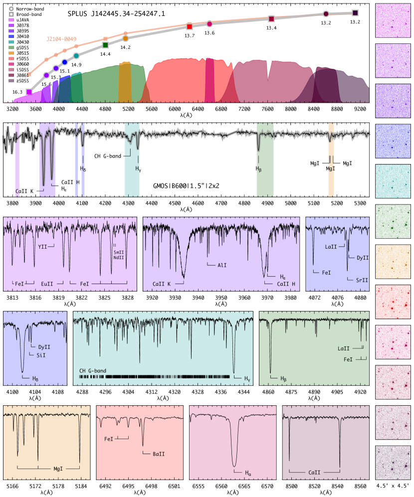
Figure 1: Top: S-PLUS magnitudes for SPLUS J1424$-$2542 (catalog )  compared to the values for SPLUS J2104$-$0049 (catalog ). Also shown are the S-PLUS filter transmission curves. The second panel from top to bottom shows the Gemini/GMOS spectrum, highlighting absorption features of interest. The remaining color panels show sections of the GHOST spectra and features used for chemical abundance determinations. The 12 side panels show the S-PLUS images for SPLUS J1424$-$2542 (catalog ). RGB colors in all panels are assigned based on the central wavelength of each filter. See text for further details.

2.1 S-PLUS and Gemini/GMOS

SPLUS J1424$-$2542 (catalog )  was observed as part of the Southern Photometric Local Universe Survey (S-PLUS; Mendes de Oliveira et al., 2019) second data release (DR2; Almeida-Fernandes et al., 2022). S-PLUS  has a unique 12 broad- and narrow-band filter set, consisting of four SDSS ($g$, $r$, $i$, $z$), one modified SDSS $u$, and seven narrow-band filters. SPLUS J1424$-$2542 (catalog )  was selected as a metal-poor star candidate by Placco et al. (2022), based on its narrow-band metallicity-sensitive colors. These colors, (J0395-J0410)-(J0660-J0861)  and (J0395-J0660)-2$\times$(g-i), are listed in Table 1 and place SPLUS J1424$-$2542 (catalog )  in the same regime as other spectroscopically confirmed low-metallicity stars (cf. Figures 1 and 7 of Placco et al., 2022). In Almeida-Fernandes et al. (2023), four criteria for the selection of metal-poor stars from S-PLUS  were proposed, resulting in different levels of completeness and purity. We note that SPLUS J1424$-$2542 (catalog )  was selected as a low metallicity candidate in all the considered cases.

The top panel of Figure 1 shows the S-PLUS  filter curves, and the twelve magnitudes (AB system) for SPLUS J1424$-$2542 (catalog ). Image cutouts for each filter ($4.5^{\prime}$x$4.5^{\prime}$ centered at SPLUS J1424$-$2542 (catalog )) are shown on the right side of the figure. RGB colors are assigned based on the central wavelength of each filter. As a comparison, the S-PLUS  magnitudes (scaled to the zSDSS value for SPLUS J1424$-$2542 (catalog )) for SPLUS J2104$-$0049 (catalog ), an ultra metal-poor star with $[\mathrm{Fe}/\mathrm{H}]$=$-4.03$ (Placco et al., 2021c), are shown. Both stars have similar temperatures, meaning that the differences in flux for the blue filters can be attributed to lower emerging flux for SPLUS J1424$-$2542 (catalog )  due to the presence of absorption features, a consequence of its overall higher chemical abundances when compared to SPLUS J2104$-$0049 (catalog ).

Medium-resolution (R $\sim 1,500$) spectroscopy for SPLUS J1424$-$2542 (catalog )  was gathered on June 18, 2021, with the 8.1 m Gemini South telescope and the GMOS (Gemini Multi-Object Spectrograph; Davies et al., 1997; Gimeno et al., 2016) instrument, as part of the Poor Weather program GS-2021A-Q-419. Further details on the observing setup and data reduction are given in Placco et al. (2022). The second panel from top to bottom on Figure 1 shows the normalized GMOS data, highlighting a few absorption features of interest for the determination of the effective temperature ($T_{\mathrm{eff}}$  – Balmer lines H$\beta$, H$\gamma$, and H$\delta$), metallicity ($[\mathrm{Fe}/\mathrm{H}]$–Ca II K), carbon abundance (CH G-band), and $\alpha$-element abundance (Mg I b triplet). The atmospheric parameters determined by Placco et al. (2022) are provided in Table 1. Based on these parameters, SPLUS J1424$-$2542 (catalog )  was selected as a potential candidate for high-resolution spectroscopic follow-up.

2.2 Gemini/GHOST

SPLUS J1424$-$2542 (catalog )  was followed up in high resolution using the newly commissioned GHOST (Gemini High-resolution Optical SpecTrograph; Ireland et al., 2014; McConnachie et al., 2022; Hayes et al., 2023) at Gemini South. Observations were conducted on May 10, 2023, as part of the GHOST SV (System Verification - Program ID: GS-2023A-SV-101) and the data is publicly available at the Gemini Observatory Archive. The instrument setup chosen was the standard resolution (SR: R $\sim 50,000$) and target mode IFU1:Target—IFU2:Sky. For both the blue and red cameras, six 900-second exposures were taken with a 1x2 binning (spectral x spatial). During the observations, the image quality (IQ) and cloud cover (CC) were in the 70^th-percentile and the sky background (SB) was in the 50^th-percentile. The wavelength coverage is [3474:5438] Å  for the blue camera and [5209:10608] Å  for the red camera.

The data reduction was performed using v3.0 of the DRAGONS software package (Labrie et al., 2019, 2022). This version includes support for GHOST, based on the GHOST Data Reduction pipeline v1.0 (GHOST DR - originally described in Ireland et al., 2018; Hayes et al., 2022), which was modified by the DRAGONS team during the commissioning of GHOST. The reduction steps included bias/flat corrections, wavelength calibration, sky subtraction, barycentric correction, extraction of individual orders, and variance-weighted stitching of the spectral orders. The six individual exposures were combined using a simple mean without rejection. The signal-to-noise ratios per pixel achieved in selected regions of the spectrum are listed in Table 1. The colored panels on Figure 1 show sections of the GHOST data (after normalization and radial velocity shift), highlighting absorption features of interest for the determination of stellar atmospheric parameters and chemical abundances, as described in Section 3.

3 Atmospheric Parameters and Chemical Abundances

3.1 Atmospheric Parameters

The stellar atmospheric parameters (effective temperature – $T_{\mathrm{eff}}$, surface gravity – $\log\,g$, and metallicity – $[\mathrm{Fe}/\mathrm{H}]$) for SPLUS J1424$-$2542 (catalog )  were first calculated by Placco et al. (2022) using the Gemini/GMOS data and the methods described therein. These parameters ($T_{\mathrm{eff}}$=4700 K, $\log\,g$=1.48, $[\mathrm{Fe}/\mathrm{H}]$=$-3.82$) were used to select SPLUS J1424$-$2542 (catalog )  as a potential candidate for high-resolution spectroscopic follow-up.

In this work, the $T_{\mathrm{eff}}$  for SPLUS J1424$-$2542 (catalog ) was calculated from the color-$T_{\mathrm{eff}}$-$[\mathrm{Fe}/\mathrm{H}]$  relations derived by Mucciarelli et al. (2021). We used the same procedure outlined in Roederer et al. (2018b), drawing 10⁵ samples for magnitudes, reddening, and metallicity. The $G$, $BP$, and $RP$ magnitudes were retrieved from the third data release of the Gaia mission (DR3; Gaia Collaboration et al., 2022a) and the $K$ magnitude from 2MASS (Skrutskie et al., 2006). The final $T_{\mathrm{eff}}$=$4762\pm 36$ K is the weighted mean of the median temperatures for each input color ($BP-RP$, $BP-G$, $G-RP$, $BP-K$, $RP-K$, and $G-K$). The $\log\,g$  was calculated using Equation 1 in Roederer et al. (2018b), drawing 10⁵ samples from the input parameters listed in Table 1. The final $\log\,g$=$1.58\pm 0.11$ is taken as the median of those calculations with the uncertainty given by their standard deviation.

The metallicity was determined spectroscopically from the equivalent widths (EWs) of 104 Fe I lines in the GHOST spectrum by fixing the $T_{\mathrm{eff}}$ and $\log\,g$ determined above. Table 2 lists the lines employed in this analysis, their measured equivalent widths, and the derived chemical abundances. The EWs were obtained by fitting Gaussian profiles to the observed absorption features using standard IRAF routines, then $[\mathrm{Fe}/\mathrm{H}]$  was calculated using the latest version of the MOOG code (Sneden, 1973), employing one-dimensional plane-parallel model atmospheres with no overshooting (Castelli & Kurucz, 2004), assuming local thermodynamic equilibrium (LTE). The microturbulent velocity ($\xi$) was determined by minimizing the trend between Fe I abundances and their reduced equivalent width ($\log(\rm{EW}/\lambda$)). The final atmospheric parameters for SPLUS J1424$-$2542 (catalog )  are listed in Table 1.

Table 2: Atomic Data and Derived Abundances

Ion	$\lambda$	$\chi$	$\log\,gf$	$EW$	$\log\epsilon$ (X)	Ref.	$\Delta$
	(Å)	(eV)		(mÅ)			NLTE
CH	4313.00	$\cdots$	$\cdots$	syn	4.83	1	$\cdots$
Na I	5889.95	0.00	0.11	142.63	3.57	1	$-$0.37
Na I	5895.92	0.00	$-$0.19	118.77	3.43	1	$-$0.27
Mg I	3829.35	2.71	$-$0.23	141.24	4.80	1	0.08
Mg I	3832.30	2.71	0.25	177.79	4.72	1	0.06
Mg I	3986.75	4.35	$-$1.06	15.44	4.87	1	$\cdots$
Mg I	4167.27	4.35	$-$0.74	18.56	4.64	1	0.13
Mg I	4702.99	4.33	$-$0.44	34.70	4.65	1	0.18
Mg I	5172.68	2.71	$-$0.36	156.21	4.79	1	0.05
Mg I	5183.60	2.72	$-$0.17	177.67	4.84	1	0.04
$\cdots$	$\cdots$	$\cdots$	$\cdots$	$\cdots$	$\cdots$		$\cdots$

Note. — The complete list of absorption features and literature references are given in Table SPLUS J142445.34$-$254247.1 (catalog ): An R-Process Enhanced, Actinide-Boost, Extremely Metal-Poor star observed with GHOST .

Table 3: LTE Abundances for Individual Species

Species	$\log\epsilon_{\odot}$ (X)	$\log\epsilon$ (X)	[X/H]	[X/Fe]	$\sigma$	$N$
C	8.43	4.83	$-$3.60	$-$0.21	0.10	1
C	8.43	5.10	$-$3.33	0.06	0.10	1
Na I	6.24	3.50	$-$2.74	0.65	0.07	2
Mg I	7.60	4.75	$-$2.85	0.54	0.07	9
Al I	6.45	2.80	$-$3.65	$-$0.26	0.15	1
Si I	7.51	4.76	$-$2.75	0.64	0.15	1
Ca I	6.34	3.36	$-$2.98	0.41	0.08	11
Sc II	3.15	$-$0.02	$-$3.17	0.22	0.05	7
Ti I	4.95	1.70	$-$3.25	0.14	0.05	7
Ti II	4.95	1.94	$-$3.01	0.38	0.09	20
V II	3.93	0.97	$-$2.96	0.43	0.02	2
Cr I	5.64	1.79	$-$3.85	$-$0.46	0.10	3
Mn I	5.43	1.51	$-$3.92	$-$0.53	0.09	3
Fe I	7.50	4.11	$-$3.39	0.00	0.12	104
Fe II	7.50	4.19	$-$3.31	0.08	0.04	11
Co I	4.99	1.68	$-$3.31	0.08	0.06	3
Ni I	6.22	2.74	$-$3.48	$-$0.09	0.15	1
Zn I	4.56	1.36	$-$3.20	0.19	0.15	1
Sr II	2.87	0.37	$-$2.50	0.89	0.10	2
Y II	2.21	$-$0.74	$-$2.95	0.44	0.04	6
Zr II	2.58	$-$0.20	$-$2.77	0.62	0.04	4
Ba II	2.18	0.04	$-$2.14	1.25	0.10	3
La II	1.10	$-$1.01	$-$2.11	1.28	0.06	8
Ce II	1.58	$-$0.63	$-$2.21	1.18	0.06	10
Pr II	0.72	$-$1.15	$-$1.87	1.52	0.02	3
Nd II	1.42	$-$0.58	$-$2.00	1.39	0.04	22
Sm II	0.96	$-$0.92	$-$1.88	1.51	0.08	17
Eu II	0.52	$-$1.25	$-$1.77	1.62	0.05	8
Gd II	1.07	$-$0.74	$-$1.81	1.58	0.04	9
Tb II	0.30	$-$1.35	$-$1.65	1.74	0.20	1
Dy II	1.10	$-$0.47	$-$1.57	1.82	0.12	9
Ho II	0.48	$-$1.33	$-$1.81	1.58	0.08	3
Er II	0.92	$-$0.80	$-$1.72	1.67	0.06	4
Tm II	0.10	$-$1.65	$-$1.75	1.65	0.08	4
Yb II	0.84	$-$1.06	$-$1.90	1.49	0.20	1
Hf II	0.85	$-$1.15	$-$2.00	1.39	0.20	1
Os I	1.40	$-$0.21	$-$1.61	1.78	0.04	2
Ir I	1.38	$-$0.35	$-$1.73	1.66	0.20	1
Th II	0.02	$-$1.21	$-$1.23	2.16	0.06	3

Table 4: Example Systematic Abundance Uncertainties for SPLUS J1424$-$2542 (catalog )

Elem	$\Delta$$T_{\mathrm{eff}}$	$\Delta$$\log\,g$	$\Delta\xi$	$\sigma$	$\sigma_{\rm tot}$
	$+$150 K	$+$0.3 dex	$+$0.3 km/s
Na I	0.18	$-$0.06	$-$0.13	0.07	0.24
Mg I	0.13	$-$0.06	$-$0.05	0.07	0.17
Ca I	0.10	$-$0.02	$-$0.02	0.08	0.13
Sc II	0.09	0.07	$-$0.03	0.05	0.13
Ti I	0.18	$-$0.02	$-$0.02	0.05	0.19
Ti II	0.08	0.08	$-$0.05	0.09	0.15
Cr I	0.19	$-$0.03	$-$0.08	0.10	0.23
Mn I	0.22	$-$0.03	$-$0.13	0.09	0.27
Fe I	0.16	$-$0.02	$-$0.04	0.12	0.20
Fe II	0.02	0.08	$-$0.01	0.04	0.09
Co I	0.20	$-$0.02	$-$0.07	0.06	0.22
Ni I	0.17	$-$0.01	$-$0.02	0.15	0.23

Table 5: NLTE Abundances for Individual Species

Species	$\log\epsilon_{\odot}$ (X)	$\log\epsilon$ (X)	[X/H]	[X/Fe]	$\sigma$	$N$
Na I	6.24	3.18	$-$3.06	0.15	0.03	2
Mg I	7.60	4.83	$-$2.77	0.44	0.05	8
Al I	6.45	3.80	$-$2.65	0.51	0.15	1
Si I	7.51	4.79	$-$2.72	0.51	0.15	1
Ca I	6.34	3.64	$-$2.70	0.41	0.07	9
Ti I	4.95	2.30	$-$2.65	0.56	0.06	6
Ti II	4.95	2.04	$-$2.91	0.30	0.10	19
Cr I	5.64	2.49	$-$3.15	0.06	0.06	3
Mn I	5.43	1.83	$-$3.60	$-$0.39	0.08	3
Fe I	7.50	4.29	$-$3.21	0.00	0.13	102
Co I	4.99	2.47	$-$2.52	0.69	0.02	3

Note. — The complete list of literature references for the NLTE corrections is given in Table SPLUS J142445.34$-$254247.1 (catalog ): An R-Process Enhanced, Actinide-Boost, Extremely Metal-Poor star observed with GHOST .

3.2 Chemical Abundances

The GHOST spectrum allowed for the detection of 308 absorption features for 36 elements, spanning the wavelength range $3694\leq\lambda(\textrm{\AA})\leq 8807$. Abundances were determined from equivalent-width analysis and spectral synthesis, both using MOOG. These features and their atomic data are listed in Table 2. Linelists for each abundance determination through spectral synthesis were generated using the linemake code (Placco et al., 2021a, b). Logarithmic abundances by number ($\log\epsilon$(X)) and abundance ratios ($[\mathrm{X}/\mathrm{H}]$ and $[\mathrm{X}/\mathrm{Fe}]$), were calculated adopting the solar photospheric abundances ($\log\epsilon_{\odot}$ (X)) from Asplund et al. (2009). The average abundances and the number of lines measured ($N$) for each element are given in Table 3. The $\sigma$ values are the standard error of the mean. For elements with only one line measured, the uncertainty was estimated by minimizing the residuals between the GHOST data and a set of synthetic spectra through visual inspection.

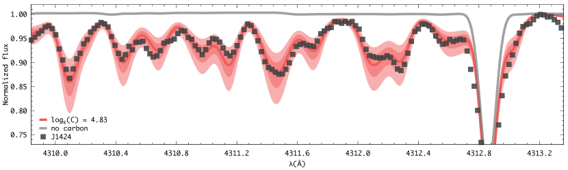
Figure 2: Spectral synthesis for the determination of the carbon abundance. The red solid line shows the best-fit synthesis and uncertainties ($\pm 0.1$ and $\pm 0.2$ dex - shaded regions) compared to the observed spectra (filled squares). Also shown is a synthetic spectrum after removing all contributions from carbon (gray line).

We have also quantified the systematic uncertainties due to changes in the atmospheric parameters for the elements with $6<Z\leq 30$ with abundances determined by equivalent analysis only (see details below), following the prescription described in Placco et al. (2013, 2015b). Table 4 shows the derived abundance variations when each atmospheric parameter is varied within the quoted uncertainties. Also listed is the total uncertainty for each element, calculated from the quadratic sum of the individual error estimates. The adopted variations for the parameters are $+$150 K for $T_{\mathrm{eff}}$, $+$0.3 dex for $\log\,g$, and $+$0.3 km s^-1 for $\xi$.

3.2.1 From C to Zn

Apart from C, Al, Si, V, and Zn, all the abundances for elements with $Z\leq 30$ were measured from equivalent widths. The carbon abundance was determined from the CH G-band spectral synthesis, assuming ${}^{12}\rm{C}/^{13}\rm{C}=4$. Figure 2 shows the GHOST spectrum (filled squares) compared to the synthetic data. The red solid line shows the best-fit synthesis and the shaded regions at $\pm 0.1$ and $\pm 0.2$ dex are used to determine the uncertainty. Also shown is a synthetic spectrum after removing all contributions from carbon (gray line). The carbon depletion on the giant branch for SPLUS J1424$-$2542 (catalog )  ($+0.27$ dex) was determined using the procedures described by Placco et al. (2014).

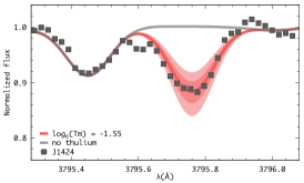
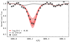
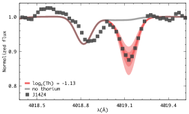
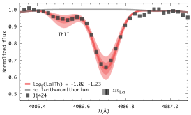
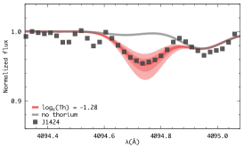
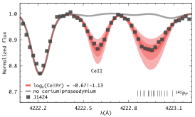
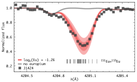
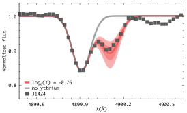
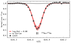
Figure 3: Same as Figure 2, for the heavy elements highlighted in each panel.

For the remaining light elements, there is an overall good agreement among the abundances of individual lines for a given species, which can be seen from the small $\sigma$ values listed in Table 3. We have also obtained non-LTE (NLTE) corrections for 157 absorption features in the spectrum of SPLUS J1424$-$2542 (catalog ), using INSPECT (Na I), Nordlander & Lind (2017) (Al I), and MPIA NLTE (Mg I, Si I, Ca I, Ti I, Ti II, Cr I, Mn I, Fe I, and Co I). Literature references are given in Table SPLUS J142445.34$-$254247.1 (catalog ): An R-Process Enhanced, Actinide-Boost, Extremely Metal-Poor star observed with GHOST along with the corrections for individual lines in the last column. Average NLTE abundances, abundance ratios, and $\sigma$ values are given in Table 5. The average NLTE corrections range from $-0.32$ for Na I to $+1.0$ for Al I, with notably high corrections also for Cr I and Co I ($+0.79$ and $+0.70$, respectively). Due to the overall low metallicity (and low carbon abundance) of SPLUS J1424$-$2542 (catalog ), most lines have a well-defined continuum and are not blended with other species (see, for example, Mg I and Ca II in the lower panels of Figure 1). Unless otherwise noted, we use the LTE abundances from Table 3 for the remainder of this work.

3.2.2 From Sr to Th

The spectral synthesis of 121 absorption features was conducted for 21 chemical species with $Z\geq 38$ and summarized in Table 3. Where appropriate, we accounted for line broadening by isotopic shifts and hyperfine splitting structure. For all syntheses, we fixed the abundances of carbon, iron, and the ¹²C/¹³C ratio. We also used the $r$-process isotopic fractions from Sneden et al. (2008) for specific elements, as described below. Figures 3 and 4 show the spectral synthesis for selected heavy elements. Symbols and lines have the same meaning as those shown in Figure 2.

Strontium, yttrium, zirconium

For these first-peak elements, there is an excellent agreement between the abundances for individual lines. Both Sr lines ($\lambda$4077 and $\lambda$4215) were fit with the same abundance ($\log\epsilon\,(\mathrm{Sr})$=0.37) and the spread is small for the six Y lines (0.12 dex) and four Zr lines (0.10 dex). The synthesis for one of the Y lines is shown in Figure 3.

Barium, lanthanum

These second-peak elements have low $r$-process fractions (Ba:15%, La:25% – Burris et al., 2000) in the Solar System. For Ba, the strongest lines($\lambda$4554 and $\lambda$4934) appear saturated and were not considered in the analysis. The three Ba lines measured at redder wavelengths agree within 0.20 dex, with an average $\log\epsilon\,(\mathrm{Ba})$=$+0.04$. For La, the eight lines measured also agree within 0.20 dex, with an average of $\log\epsilon\,(\mathrm{La})$=$-1.01$. The syntheses for the Ba ($\lambda$6141) and La ($\lambda$4086 – including hyperfine splitting) lines are shown in Figure 3.

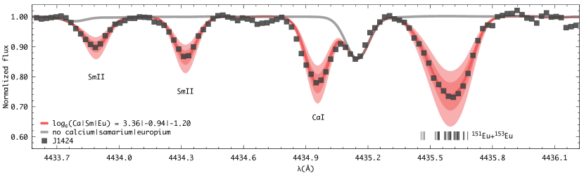
Figure 4: Same as Figure 2, for samarium, calcium, and europium abundance determinations.

Cerium, praseodymium, neodymium, samarium

These elements have a large number of lines identified at wavelengths $\lambda\leq$4600Å  (see Roederer et al., 2018b, for a comprehensive list). In total, 52 lines were measured in the GHOST spectrum of SPLUS J1424$-$2542 (catalog ), with standard deviations $\sigma\leq 0.08$. Figure 4 shows the synthesis for two Sm lines and Figure 3 shows the synthesis for Ce and Pr (including hyperfine splitting).

Europium

This is one of the most widely used elements to indicate $r$-process nucleosynthesis and it is used to classify stars into various categories for heavy-element signatures (Frebel, 2018). Eight lines were measured in the GHOST spectrum, ranging from $\lambda$3724 ($\log\epsilon\,(\mathrm{Eu})$=$-1.17$) to $\lambda$6645 ($\log\epsilon\,(\mathrm{Eu})$=$-1.23$). Two examples of Eu spectral synthesis are shown in Figure 3 ($\lambda$4205) and Figure 4 ($\lambda$4435). In both cases, there is an overall good agreement between the observations (filled symbols) and the best synthetic fit (red lines). The final average is $\log\epsilon\,(\mathrm{Eu})$=$-1.25$ ($[\mathrm{Eu}/\mathrm{Fe}]$=$+1.62$).

Gadolinium, terbium, dysprosium, holmium, erbium, thulium, ytterbium, hafnium

These elements, with $64\leq Z\leq 72$, are mostly formed by the $r$-process, according to the fractions in Burris et al. (2000). In total, 32 lines were measured within this group (most at $\lambda\leq$4000Å, with only one feature for Tb ($\lambda$3874), Yb ($\lambda$3694), and Hf ($\lambda$4093). There were nine Dy lines measured with a somewhat high dispersion ($\sigma$=0.12 dex) and good agreement for Gd (9 lines – $\sigma=0.04$), Ho (3 lines – $\sigma=0.08$), Er (4 lines – $\sigma=0.06$), and Tm (4 lines – $\sigma=0.08$). The top panels of Figure 3 show the syntheses for Tm ($\lambda$3795) and Er ($\lambda 3896$) lines.

Osmium, iridium

These third-peak elements are almost exclusively formed by the $r$-process in the Solar System (Os:92%, Ir:99% – Burris et al., 2000) and also don’t have many lines available for abundance determination in the spectral range of the GHOST data. The abundances for the two Os lines ($\lambda$4260 and $\lambda 4420$) agree within 0.07 dex, with an average of $\log\epsilon\,(\mathrm{Os})$=$-0.21$. Only one Ir line was identified in SPLUS J1424$-$2542 (catalog )  ($\lambda$3800), with an abundance of $\log\epsilon\,(\mathrm{Ir})$=$-0.35$.

Thorium

As a radioactive actinide with $Z=90$, Th is the second heaviest element with abundances measured in stellar spectra. For SPLUS J1424$-$2542 (catalog ), three lines were identified in the GHOST spectrum: $\lambda$4019 ($\log\epsilon\,(\mathrm{Th})$=$-1.13$), $\lambda$4086 ($\log\epsilon\,(\mathrm{Th})$=$-1.23$), and $\lambda$4094 ($\log\epsilon\,(\mathrm{Th})$=$-1.28$). Their spectral syntheses are shown in Figure 3. For the $\lambda$4019 line, the abundances of C, Fe, Ni, Ce, and Nd were held constant using the average values in Table 3, and there appears to be a reduction artifact on the blue wing of the Th line. The La abundance was also held constant for the $\lambda$4086 synthesis. The GHOST spectrum was slightly smoothed (with a moving average of size 5 pixels) for the synthesis of the $\lambda$4094 line. The final average is $\log\epsilon\,(\mathrm{Th})$=$-1.21$.

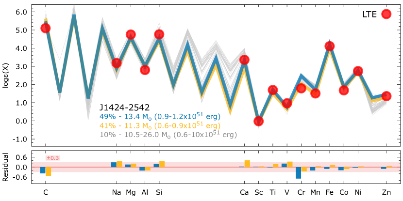
Figure 5: Upper panel: light-element chemical abundance pattern of SPLUS J1424$-$2542 (catalog ), (filled circles, LTE) compared with yields from metal-free supernova models (solid lines). The labels show the progenitor mass and explosion energy of the models and their percentage occurrence among the 10,000 abundance pattern resamples of SPLUS J1424$-$2542 (catalog ). Lower panel: residuals between observations and the two best-fit models. A $\pm$0.3 dex shaded area is shown for reference.

4 The Chemo-dynamical Nature of SPLUS J1424$-$2542 (catalog )

In this section, we discuss the chemo-dynamical nature of SPLUS J1424$-$2542 (catalog )  by comparing its chemical abundance pattern with Pop III supernova nucleosynthesis yields ($Z\leq 30$), the $r$- and $s$- process solar fractions, and predictions from a simulation of neutron star mergers ($Z\geq 38$). We also determine the mass, age, and orbit for SPLUS J1424$-$2542 (catalog ), in an attempt to constrain its formation history.

4.1 The Light-element Abundance Pattern

At $[\mathrm{Fe}/\mathrm{H}]$=$-3.39$, $[\mathrm{C}/\mathrm{Fe}]$=$+0.06$, and with enhancements in heavy elements, SPLUS J1424$-$2542 (catalog ) most likely was formed from a gas cloud polluted by at least two progenitor populations. To corroborate that hypothesis, the $[\mathrm{Mg}/\mathrm{C}]$ abundance ratio from Hartwig et al. (2018) can be used as a diagnostic to distinguish between mono- and multi-enriched stars. For SPLUS J1424$-$2542 (catalog ), both the observed and natal values ($[\mathrm{Mg}/\mathrm{C}]$=$+0.75$ and $+0.48$, respectively) are consistent with the multi-enriched classification (Figure 11 of Hartwig et al., 2018).

Nonetheless, we can attempt to infer the main features of the progenitor population that enriched the gas cloud that formed SPLUS J1424$-$2542 (catalog )  with elements from carbon to zinc. We modeled the light-element abundance signature of SPLUS J1424$-$2542 (catalog ) by comparing it with the theoretical Pop III supernova nucleosynthesis yields from Heger & Woosley (2010). These models predict the nucleosynthesis products of massive metal-free stars with pristine Big Bang nucleosynthesis initial composition, without mass loss and rotation throughout the evolution. The fallback models (S4) used in this work have masses from 10 to 100 M_⊙ and explosion energies ranging from $0.3\times 10^{51}$ erg to $10\times 10^{51}$ erg. The comparison between models and observations, as well as the $\chi^{2}$ matching algorithm, has already been applied to EMP stars in the literature (Frebel et al., 2015; Roederer et al., 2016; Placco et al., 2020, among others) and provides important constraints on the progenitor population of second-generation stars.

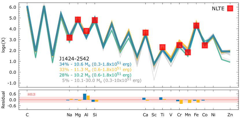
Figure 6: Same as Figure 5, using the NLTE abundances listed in Table 5.

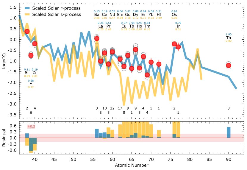
Figure 7: Upper panel: heavy-element chemical abundance pattern of SPLUS J1424$-$2542 (catalog ), compared with the scaled solar system abundances. The r- and s-process contributions are calculated based on the fractions given by Burris et al. (2000) and scaled to match the observed abundances of Eu and Ba, respectively. Also shown are the r- and s- process fractions for each element (top), as well as the number of lines identified for each element (bottom). Open circles show the individual abundances for all the lines measured in the GHOST spectrum. Lower panel: residuals between observations and the scaled solar system abundance patterns. A $\pm$0.2 dex shaded area is shown for reference.

Similar to Placco et al. (2016), we created 10,000 abundance patterns for SPLUS J1424$-$2542 (catalog ), by re-sampling the $\log\epsilon(\mbox{X})$ and $\sigma$ values from Table 3. By determining the best-fit model for each re-sampled pattern using the LTE abundances, we found that 36 unique models provided an acceptable fit for at least 10 re-samples. The results of this exercise are shown in Figure 5. In the upper panel, the filled circles show the chemical abundances for SPLUS J1424$-$2542 (catalog )  and the lines represent the different models used for the fitting. The labels show the percentage occurrence for the most frequent models among the 10,000 runs. The bottom panel shows the residuals between observations and the three most frequent models.

The “best-fit” result found in 49% of the re-samples is a model with 13.4 M_⊙ [$0.9-1.2\times 10^{51}$ erg], followed by 11.3 M_⊙ [$0.6-0.9\times 10^{51}$ erg] in 41% of the re-samples. There is an overall good agreement between the two best-fit models and the observed abundances for SPLUS J1424$-$2542 (catalog ), with a somewhat large ($\geq+0.3$ dex) residual for carbon and chromium. It is interesting to note that, out of the 10,000 re-samples, about 90% have their best-fit model for either $13.4\,M_{\odot}$ or $11.3\,M_{\odot}$ within a narrow range of explosion energies.

We repeated this exercise for the NLTE abundances in Table 5 and the results are shown in Figure 6. For the set of ten elements (as opposed to 15 in LTE), the most likely Pop. III characteristics are very similar to the LTE case, with a preference for lower masses and explosion energies. For 34% of the re-samples, 10.6 M_⊙ progenitors provide the best fit, followed by the 11.3 M_⊙ (33%) and 10.2 M_⊙ (28%) models, all with explosion energies within $0.3-1.8\times 10^{51}$ erg. Even though these results agree well with the LTE analysis, it is worth pointing out that carbon (and nitrogen) are key elements when comparing observations with the faint-SN models, as pointed out by Placco et al. (2015a). Additional abundance determinations and NLTE corrections would help further constrain these models.

For both the LTE and NLTE abundance patterns, this exercise suggests that a progenitor star on the low-mass end of the SN grid with low explosion energy could be responsible for the light-element abundance pattern of SPLUS J1424$-$2542 (catalog ). This mass range and explosion energies are not consistent with the progenitor population suggested for stars with similar low carbon abundances: 30 M_⊙ for SPLUS J2104$-$0049 (catalog )  (Placco et al., 2021a) and 20 M_⊙ for AS0039 (Skúladóttir et al., 2021), both with explosion energy of $10\times 10^{51}$ erg. This may be a metallicity effect since these stars are in the $[\mathrm{Fe}/\mathrm{H}]$$<-4$ regime, so further exploration of the progenitor population of EMP stars would help better constrain their main characteristics.

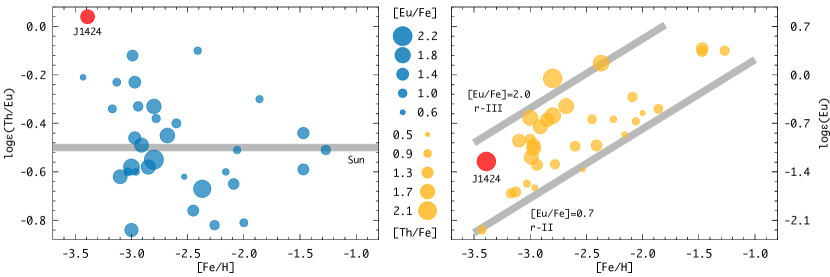
Figure 8: $\log\epsilon\,(\mathrm{Th/Eu})$ (left panel) and $\log\epsilon\,(\mathrm{Eu})$ (right panel) as a function of $[\mathrm{Fe}/\mathrm{H}]$  for metal-poor stars in the literature with both Th and Eu measured ($[\mathrm{Fe}/\mathrm{H}]$$\leq-1.0$ and $[\mathrm{Eu}/\mathrm{Fe}]$$\geq+0.60$), compared to SPLUS J1424$-$2542 (catalog ). The point sizes are proportional to $[\mathrm{Eu}/\mathrm{Fe}]$ (left) and $[\mathrm{Th}/\mathrm{Fe}]$ (right), according to the labels between the panels. The horizontal solid gray line marks the solar $\log\epsilon\,(\mathrm{Th/Eu})$ value and on the right panel, the limits for the $r$-II and $r$-III stars are shown. Individual references are given in Table 6.

4.2 The Heavy-element Abundance Pattern

With $[\mathrm{Eu}/\mathrm{Fe}]$=$+1.62$ and $[\mathrm{Ba}/\mathrm{Eu}]$=$-0.37$ abundance ratios, SPLUS J1424$-$2542 (catalog )  is classified as an $r$-II metal-poor star (Frebel, 2018), with a clear signature of the main r-process. Its heavy-element abundance pattern, compared to the Solar System $s$-process (scaled to Ba) and $r$-process (scaled to Eu), is shown in the upper panel of Figure 7. Filled circles are the average abundance for each element, while empty circles show the abundances for all the lines measured in the GHOST spectrum. Each label shows the element symbol and its $s$ and $r$ fractions, taken from Burris et al. (2000). Also shown are the number of lines used to calculate the average abundance for each element. The lower panel shows the residuals between observations and the scaled patterns. For reference, the red shaded area denotes the typical uncertainty ($\sim 0.2$ dex) in the abundance measurements.

Sr, Y, and Zr agree with neither the scaled $s$ nor $r$ patterns for SPLUS J1424$-$2542 (catalog ). These elements are formed mainly by the $s$-process in the stars whose metals enriched the Sun. However, there are a number of possible formation channels for these light neutron-capture elements (dubbed as “limited” r-process), which could help explain their large variation, when compared with the normalized $r$-process patterns among low-metallicity stars (see Table 2 and Figure 5 in Frebel, 2018). For Ba, La, and Ce, there is a clear over-production when compared to the scaled $r$-process pattern, which could suggest a contribution from the $s$-process to the observed abundance pattern of SPLUS J1424$-$2542 (catalog ). This contribution would be revealed by abundance ratios such as $[\mathrm{Ba}/\mathrm{Eu}]$ and $[\mathrm{La}/\mathrm{Eu}]$, which are expected to be $\gtrsim 0.0$ if an $s$-process component is present (Roederer et al., 2010; Frebel, 2018). For SPLUS J1424$-$2542 (catalog ), both ratios are consistent with the $r$-process expectation (and $[\mathrm{Ba}/\mathrm{Eu}]$=$-0.37$ and $[\mathrm{La}/\mathrm{Eu}]$=$-0.34$).

In contrast, the abundances for elements from Pr to Ir well reproduce the normalized $r$-process pattern, mostly within 1-$\sigma$ (with the exception of Dy). Apart from those, thorium has a measured abundance that is over 0.5 dex higher than the normalized $r$-process pattern. This “actinide boost” phenomenon is shared by about a quarter of metal-poor stars with measurable Th (and U) and it could be evidence of either a contribution from a separate $r$-process event or small variations of neutron richness within the same type of $r$-process event that contributed to the abundance make up of SPLUS J1424$-$2542 (catalog )  (Holmbeck et al., 2018, 2019).

Figure 8 shows the heavy element abundance ratio $\log\epsilon\,(\mathrm{Th/Eu})$ (left panel) and $\log\epsilon\,(\mathrm{Eu})$ (right panel) as a function of $[\mathrm{Fe}/\mathrm{H}]$  for stars in the literature with $[\mathrm{Fe}/\mathrm{H}]$$\leq-1.0$, $[\mathrm{Eu}/\mathrm{Fe}]$$\geq+0.6$, and both Th and Eu measured, compared to SPLUS J1424$-$2542 (catalog ). The point sizes are proportional to $[\mathrm{Eu}/\mathrm{Fe}]$ (left) and $[\mathrm{Th}/\mathrm{Fe}]$ (right). From the left panel, it is possible to see that SPLUS J1424$-$2542 (catalog )  has the highest $\log\epsilon\,(\mathrm{Th/Eu})$ within this group (well above the solar value - solid gray line) and the second lowest $[\mathrm{Fe}/\mathrm{H}]$, which corroborates with the hypothesis that it belongs to the “actinide boost” category and that its heavy elements have been produced by an $r$-process event without contributions from the $s$-process. The right panel also reveals that SPLUS J1424$-$2542 (catalog )  has one of the highest $[\mathrm{Th}/\mathrm{Fe}]$ ratios and the lowest metallicity among the $r$-II stars, and similar $[\mathrm{Th}/\mathrm{Fe}]$ to the $r$-III star ($[\mathrm{Eu}/\mathrm{Fe}]$$\geq+2.0$) from Cain et al. (2020). In the following section, we present one possible scenario that can explain the heavy-element abundance pattern in SPLUS J1424$-$2542 (catalog ).

4.3 Comparison with Yields from Neutron-Star Neutron-Star Merger Event

Similarly to the exercise in Section 4.1 for the light elements, we explore the origin of the heavy elements in SPLUS J1424$-$2542 (catalog )  made by the $r$-process. Specifically, we use the analytic model of Holmbeck et al. (2021) to find which neutron star mergers can reproduce the observed abundance pattern of SPLUS J1424$-$2542 (catalog ). This model predicts the total $r$-process yield for a neutron star merger using the neutron star masses and a nuclear equation of state (which determines their stellar radii) as input. The total $r$-process yield is found by assuming a two-component ejecta scheme: a “wind” and a “dynamical” component. The ejecta masses and compositions of the two components are calculated following the procedure and default model assumptions in Holmbeck et al. (2021), namely that the ejecta masses of the wind and dynamical components follow the descriptions in Dietrich et al. (2020) and Krüger & Foucart (2020), respectively. We require the model output to match the relative light-to-heavy and actinide-to-heavy abundance features present in the abundance pattern of SPLUS J1424$-$2542 (catalog ), represented by the observational $\log\epsilon\,(\mathrm{Zr/Dy})$ and $\log\epsilon\,(\mathrm{Th/Dy})$ abundance ratios. Using the nuclear equation of state proposed by Holmbeck et al. (2022), we find that a 1.66–1.27 M_☉ neutron star merger best reproduces these abundance ratios.

Including observational uncertainties, the neutron star masses can vary within $\pm$0.02 M_☉ and still be able to match the elemental abundances in SPLUS J1424$-$2542 (catalog ). The model predicts median masses and lanthanide mass fractions of $m_{\rm disk}=7.15_{-2.50}^{+2.96}\times 10^{-3}$ M_⊙ with $X_{\rm disk}^{\rm lan}=0.050_{-0.017}^{+0.019}$ and $m_{\rm dyn}=11.79_{-1.64}^{+1.40}\times 10^{-3}$ M_⊙ with $X_{\rm dyn}^{\rm lan}=0.143_{-0.005}^{+0.005}$ for the disk and dynamical components, respectively. The model prefers a somewhat high total binary mass (2.93 M_⊙) and mass ratio ($M_{1}/M_{2}=1.31$) in order to minimize the light-to-heavy and maximize the actinide-to-heavy abundance ratios. The high total mass promotes a prompt collapse, maximizing the neutron-richness of the wind ejecta while also minimizing its total ejecta mass. This twofold effect serves to suppress the first $r$-process peak in favor of the heavy $r$-process elements: necessary in the present case of the relatively low first-peak abundances of SPLUS J1424$-$2542 (catalog ). At the same time, the high neutron star mass ratio promotes a high dynamical ejecta mass, which also serves to lower the light-to-heavy abundance ratio by diluting the wind ejecta with very neutron-rich dynamical ejecta that favors actinide production.

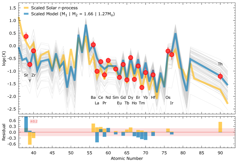
Figure 9: Upper panel: heavy-element chemical abundance pattern of SPLUS J1424$-$2542 (catalog ), compared with the scaled solar system $r$-process (yellow) and the best-fit neutron star merger model (blue), normalized to match the observed europium abundance. Also shown (gray lines) are random realizations of the neutron star merger, see text for details. Lower panel: residuals between observations and scaled predictions. A $\pm$0.2 dex shaded area is shown for reference.

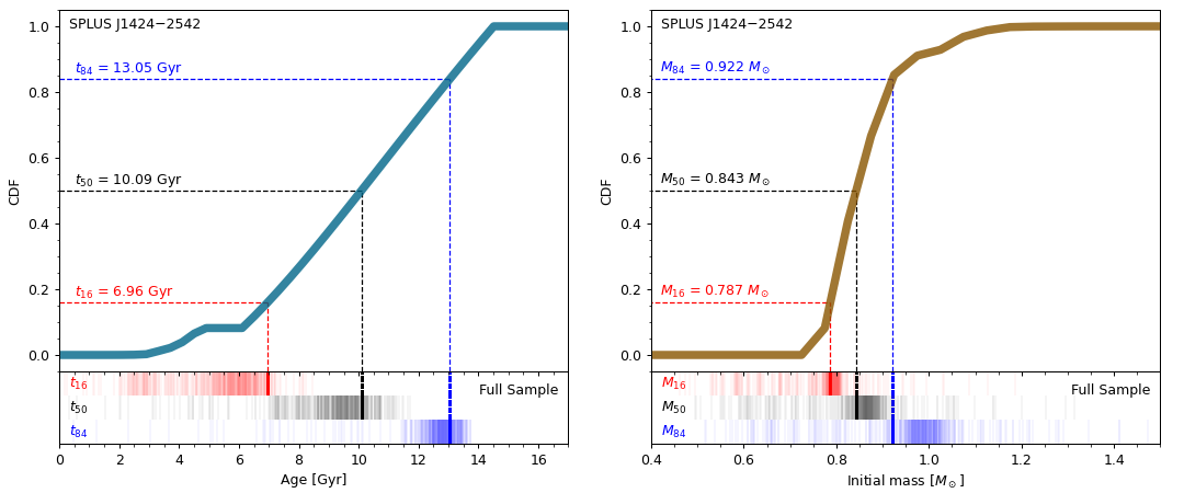
Figure 10: Age (left) and initial mass (right) cumulative distribution functions obtained for SPLUS J1424$-$2542 (catalog )  using the Bayesian isochronal method described in Almeida-Fernandes et al. (2023). The dashed lines correspond to the 16th (red), 50th (black), and 84th (blue) percentiles used to characterize the parameters and their uncertainties. For comparison, the ticks in the bottom panels correspond to the 16th (red), 50th (black), and 84th (blue) percentiles for all 522 stars in the Placco et al. (2022) sample.

Figure 9 shows the heavy-element abundance pattern of the best-fit neutron star merger model (blue) compared to SPLUS J1424$-$2542 (catalog )  (red) and the scaled Solar $r$-process abundance pattern (yellow). The analytic model is not without its own uncertainties; also shown in Figure 9 are the chemical abundance patterns of 100 random realizations of a 1.66–1.27 M_☉ neutron star merger (gray lines). These uncertainties reflect those of the analytic forms of the ejecta masses described in Dietrich et al. (2020) and Krüger & Foucart (2020) (see Holmbeck et al., 2022, for details). Even though there are still some discrepancies between the theoretical predictions and observations (most notably for Sr, La, Tm, and Yb), this model can successfully reproduce the heavy element abundance pattern of SPLUS J1424$-$2542 (catalog ). Additional measurements from higher S/N spectra will help further constrain and refine the models.

4.4 Age and Initial Mass

In Almeida-Fernandes et al. (2023), the chemo-dynamical properties and ages of the 522 metal-poor candidates selected by Placco et al. (2022), which includes SPLUS J1424$-$2542 (catalog ), were analyzed. Below we discuss the parameters obtained for this particular star and the results are summarized in Table 1.

The age and initial mass of SPLUS J1424$-$2542 (catalog )  were estimated through a Bayesian isochronal method using the MESA Isochrones & Stellar Tracks (MIST; Dotter, 2016). Details of the process can be found in Almeida-Fernandes et al. (2023). In Figure 10 we present the cumulative distribution function (CDF) for the age (left panel) and initial mass (right panel) for SPLUS J1424$-$2542 (catalog ). These parameters were estimated from the median of the distributions (black dashed lines), and the lower and upper limits as the 16th and 84th percentiles (red and blue dashed lines, respectively). For comparison, we also show the distribution of median ages and initial masses for all 522 stars in the Placco et al. (2022) sample as black ticks in the bottom panels, as well as the distributions of 16th and 84th percentiles as red and blue ticks, respectively.

The CDF in the left panel of Figure 10 shows that the estimated age for SPLUS J1424$-$2542 (catalog )  is poorly constrained beyond 6 Gyr, i.e. the linear CDF corresponds to a very flat probability distribution at these ages. This CDF results in a very high age uncertainty, where the lower and upper limits differ from the median by about 3 Gyr. Nevertheless, the characterized median age of $10.09$ Gyr places SPLUS J1424$-$2542 (catalog )  among the top 18% oldest stars in the Placco et al. (2022) sample. The CDF in the right panel shows that the initial mass of SPLUS J1424$-$2542 (catalog )  can be much better constrained. The observed sub-solar mass of $0.843_{-0.056}^{+0.079}$ is consistent with the expectation for such an old and metal-poor star.

4.5 Kinematical Parameters

We used the photo-geometric distances provided by Bailer-Jones et al. (2021), and the proper motions and line-of-sight velocities of Gaia DR3 (Gaia Collaboration et al., 2022b) to calculate the kinematical parameters of SPLUS J1424$-$2542 (catalog ). Its Heliocentric Galactic rectangular velocity vector corresponds to $(U,V,W)=(-93,-29.4,+46.4)$ km s^-1, resulting in a total velocity of $V_{\mathrm{Tot}}=108.0$ km s^-1. In cartesian galactocentric coordinates, its current position corresponds to $(X,Y,Z)=(2.61,-3.50,4.22)$ kpc. Given its current position and total velocity, one can infer that SPLUS J1424$-$2542 (catalog )  belongs to the Galactic halo.

4.6 Galactic Orbit and Halo Substructure Membership

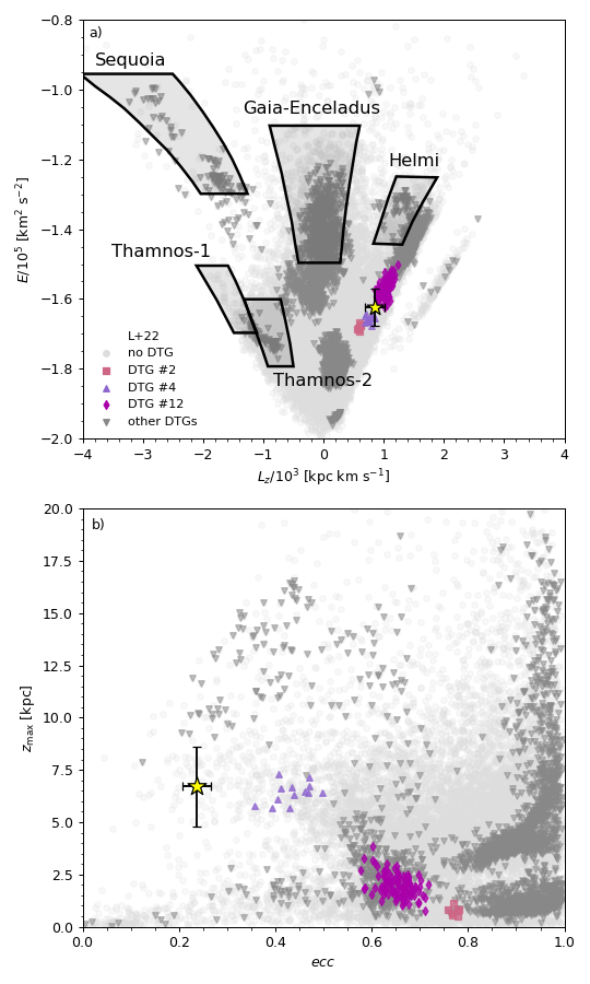
Figure 11: Top panel: comparison between the vertical component of the angular momentum and orbital energy of SPLUS J1424$-$2542 (catalog )  (yellow star-shaped symbol) to those of known halo substructures (as defined by Koppelman et al., 2019) and dynamically tagged groups (identified by Lövdal et al., 2022). Bottom panel: eccentricity and maximum distance from the galactic plane for SPLUS J1424$-$2542 (catalog )  and the stars in the Lövdal et al. (2022) sample.

The orbit of SPLUS J1424$-$2542 (catalog )  was integrated in a McMillan (2017) Galactic potential using the galpy package (Bovy, 2015). We adopted a galactocentric distance of $R_{\odot}=8.21$ kpc, with corresponding rotation velocity of $V_{\odot}=233.1$ km s^-1 (McMillan, 2017), and a Solar velocity of $(U_{\odot},V_{\odot},W_{\odot})=(11.1,12.24,7.25)$ km s^-1 (Schönrich et al., 2010). We estimated orbital parameters, such as apogalactic and perigalactic radius ($R_{\mathrm{apo}}$, $R_{\mathrm{peri}}$), maximum distance from the Galactic plane ($z_{\mathrm{max}}$), and orbital eccentricity ($ecc$). We also calculate the angular momentum, energy, and action angles, which allow us to investigate if SPLUS J1424$-$2542 (catalog )  belongs to any known Halo substructure.

In Figure 11 we compare the dynamical properties (top: $L_{z}$ vs. $E$; bottom: $ecc$ vs. $z_{\mathrm{max}}$) of SPLUS J1424$-$2542 (catalog )  (yellow star-shaped symbol) with the parameters expected for different galactic substructures, as well as 67 dynamically tagged groups (DTGs). The uncertainties for SPLUS J1424$-$2542 (catalog )  were computed from the standard deviation of the results from 5,000 orbital integrations produced using Monte Carlo re-sampling of the astrometry, distances, and radial velocities, taking into account the errors in each parameter. The shaded regions shown in the top panel correspond to the substructures of Sequoia, Thamnos-1 and Thamnos-2, Gaia-Sausage-Enceladus, and Helmi Stream, as defined by Koppelman et al. (2019). Given the observed differences in the vertical component of the angular momentum and in the energy, we can conclude that SPLUS J1424$-$2542 (catalog )  does not share the same dynamical properties as any of the known halo major substructures.

We also compare the dynamical properties of SPLUS J1424$-$2542 (catalog )  to those of 67 DTGs identified by Lövdal et al. (2022) using data from Gaia EDR3 (Gaia Collaboration et al., 2021). In Figure 11 we include the sample of Lövdal et al. (2022) (light-grey circles), and identify the stars that were assigned to any of the DTGs (grey inverted triangles). In the top panel, we highlight three DTGs that share similar $L_{z}$ and $E$ as SPLUS J1424$-$2542 (catalog ), labeled by Lövdal et al. (2022) as DTGs 2 (pink squares), 4 (violet triangles), and 12 (magenta diamonds). However, as seen in the bottom panel, SPLUS J1424$-$2542 (catalog )  does not share the same values of $ecc$ and $z_{\mathrm{max}}$ as DTGs 2 and 12. Stars in the DTG 4 have the same $z_{\mathrm{max}}$ as SPLUS J1424$-$2542 (catalog ), but the eccentricity is higher by about $0.2$. The differences between the dynamical properties of SPLUS J1424$-$2542 (catalog )  and those of known halo substructures could be indicative that this star belongs to the in-situ halo population.

5 Conclusions and Future Work

In this work, we presented the chemo-dynamical analysis of SPLUS J1424$-$2542 (catalog ), an $r$-process enhanced, actinide-boost star observed with the newly commissioned GHOST spectrograph at the Gemini South Telescope. By comparing the light- and heavy-element abundance patterns with yields from theoretical models, we speculate that the gas cloud from which SPLUS J1424$-$2542 (catalog )  was formed must have been enriched by at least two progenitor populations, the supernova explosion from a metal-free 11.3–13.4 M_⊙ star and the aftermath of a binary neutron star merger with masses 1.66 M_⊙ and 1.27 M_⊙. The mass ($0.843_{-0.056}^{+0.079}$ M_⊙) and age ($10.09_{-3.12}^{+2.96}$ Gyr) for SPLUS J1424$-$2542 (catalog )  are consistent with the proposed formation scenario and its kinematics do not connect it with any known structures in the Milky Way halo. Further identification and spectroscopic follow-up of similar objects will help increase our understanding of the formation and chemical evolution of our Galaxy. In this context, GHOST will be a valuable resource for the astronomical community.

The authors would like to thank Janice Lee, Bryan Miller, and the Gemini Observatory staff members for their contributions to the GHOST System Verification. The work of V.M.P., K.C., E.D., J.H., V.K., S.X., R.D., M.G., D.H., P.P., C.Q., R.R., C.S., C.U., Z.H., D.J., K.L., B.M., G.P., S.R., and J.T. is supported by NOIRLab, which is managed by the Association of Universities for Research in Astronomy (AURA) under a cooperative agreement with the National Science Foundation. F.A.-F. acknowledges funding for this work from FAPESP grants 2018/20977-2 and 2021/09468-1. I.U.R. acknowledges support from U.S. National Science Foundation (NSF) grants PHY 14-30152 (Physics Frontier Center/JINA-CEE), AST 1815403/1815767, AST 2205847, and the NASA Astrophysics Data Analysis Program, grant 80NSSC21K0627. K.A.V. thanks the National Sciences and Engineering Research Council of Canada for funding through the Discovery Grants and CREATE programs. M.J. acknowledges partial support from the National Research Foundation (NRF) of Korea grant funded by the Ministry of Science and ICT (NRF-2021R1A2C1008679). E.M. acknowledges funding from FAPEMIG under project number APQ-02493-22 and research productivity grant number 309829/2022-4 awarded by the CNPq, Brazil. Based on observations obtained at the International Gemini Observatory (Program IDs: GS-2021A-Q-419, GS-2023A-SV-101), a program of NSF’s NOIRLab, which is managed by the Association of Universities for Research in Astronomy (AURA) under a cooperative agreement with the National Science Foundation. on behalf of the Gemini Observatory partnership: the National Science Foundation (United States), National Research Council (Canada), Agencia Nacional de Investigación y Desarrollo (Chile), Ministerio de Ciencia, Tecnología e Innovación (Argentina), Ministério da Ciência, Tecnologia, Inovações e Comunicações (Brazil), and Korea Astronomy and Space Science Institute (Republic of Korea). Data processed using DRAGONS (Data Reduction for Astronomy from Gemini Observatory North and South). GHOST was built by a collaboration between Australian Astronomical Optics at Macquarie University, National Research Council Herzberg of Canada, and the Australian National University, and funded by the International Gemini partnership. The instrument scientist is Dr. Alan McConnachie at NRC, and the instrument team is also led by Dr. Gordon Robertson (at AAO), and Dr. Michael Ireland (at ANU). The authors would like to acknowledge the contributions of the GHOST instrument build team, the Gemini GHOST instrument team, the full SV team, and the rest of the Gemini operations team that were involved in making the SV observations a success. The S-PLUS project, including the T80-South robotic telescope and the S-PLUS scientific survey, was founded as a partnership between the Fundação de Amparo à Pesquisa do Estado de São Paulo (FAPESP), the Observatório Nacional (ON), the Federal University of Sergipe (UFS), and the Federal University of Santa Catarina (UFSC), with important financial and practical contributions from other collaborating institutes in Brazil, Chile (Universidad de La Serena), and Spain (Centro de Estudios de Física del Cosmos de Aragón, CEFCA). We further acknowledge financial support from the São Paulo Research Foundation (FAPESP), the Brazilian National Research Council (CNPq), the Coordination for the Improvement of Higher Education Personnel (CAPES), the Carlos Chagas Filho Rio de Janeiro State Research Foundation (FAPERJ), and the Brazilian Innovation Agency (FINEP). The members of the S-PLUS collaboration are grateful for the contributions from CTIO staff in helping in the construction, commissioning and maintenance of the T80-South telescope and camera. We are also indebted to Rene Laporte, INPE, and Keith Taylor for their important contributions to the project. From CEFCA, we thank Antonio Marín-Franch for his invaluable contributions in the early phases of the project, David Cristóbal-Hornillos and his team for their help with the installation of the data reduction package jype version 0.9.9, César Íñiguez for providing 2D measurements of the filter transmissions, and all other staff members for their support with various aspects of the project. IRAF was distributed by the National Optical Astronomy Observatory, which was managed by AURA under a cooperative agreement with the NSF. This research has made use of NASA’s Astrophysics Data System Bibliographic Services; the arXiv pre-print server operated by Cornell University; the SIMBAD database hosted by the Strasbourg Astronomical Data Center; and the online Q&A platform stackoverflow (http://stackoverflow.com/).

Table 6: Information for the literature comparison sample in Figure 8.

Star	$[\mathrm{Fe}/\mathrm{H}]$	$\log\epsilon\,(\mathrm{Eu})$	$\log\epsilon\,(\mathrm{Th})$	Reference
LAMOST J112456.61$+$453531.3	$-$1.27	0.35	$-$0.16	Xing et al. (2019)
HD 222925	$-$1.47	0.38	$-$0.06	Roederer et al. (2008)
COS82	$-$1.47	0.34	$-$0.25	Aoki et al. (2007)
RAVE J093730.5$-$062655	$-$1.86	$-$0.49	$-$0.79	Sakari et al. (2019)
2MJ1521$-$0607	$-$2.00	$-$0.55	$-$1.36	Sakari et al. (2018a)
BD$+$173248	$-$2.06	$-$0.67	$-$1.18	Cowan et al. (2002)
RAVE J153830.9$-$180424	$-$2.09	$-$0.32	$-$0.97	Sakari et al. (2018b)
HD 221170	$-$2.16	$-$0.86	$-$1.46	Ivans et al. (2006a)
2MJ2256$-$0719	$-$2.26	$-$0.64	$-$1.46	Sakari et al. (2018a)
2MASS J21511791$-$1233417	$-$2.37	0.17	$-$0.50	Cohen et al. (2003)
2MASS J15141890$+$0727028	$-$2.41	$-$1.02	$-$1.12	Honda et al. (2004)
J0246$-$1518	$-$2.45	$-$0.64	$-$1.40	Sakari et al. (2018a)
HD 108317	$-$2.53	$-$1.37	$-$1.99	Roederer et al. (2012)
2MASS J22310218$-$3238365	$-$2.60	$-$1.03	$-$1.43	Hayek et al. (2009)
2MASS J00280692$-$2603042	$-$2.68	$-$0.45	$-$0.90	Christlieb et al. (2004a)
2MASS J23303707$-$5626142	$-$2.78	$-$1.29	$-$1.67	Mashonkina et al. (2010b)
J1521$-$3538	$-$2.80	$-$0.05	$-$0.60	Cain et al. (2018)
BD$-$16251	$-$2.80	$-$0.59	$-$0.92	Honda et al. (2004)
CS 29497$-$004	$-$2.85	$-$0.65	$-$1.23	Hill et al. (2017)
RAVE J203843.2$-$002333	$-$2.91	$-$0.75	$-$1.24	Placco et al. (2017)
2MASS J22545856$-$4209193	$-$2.94	$-$1.30	$-$1.63	Mashonkina et al. (2014b)
HD 115444	$-$2.96	$-$1.63	$-$2.23	Westin et al. (2000)
J1432$-$4125	$-$2.97	$-$1.01	$-$1.47	Cain et al. (2018)
2MASS J12213413$-$0328396	$-$2.97	$-$1.06	$-$1.29	Hayek et al. (2009)
2MASS J09544277$+$5246414	$-$2.99	$-$1.19	$-$1.31	Holmbeck et al. (2018)
TYC 5594$-$576$-$1	$-$3.00	$-$0.62	$-$1.20	Frebel et al. (2007)
DES J033523$-$540407	$-$3.00	$-$0.93	$-$1.77	Ji & Frebel (2018)
J2005$-$3057	$-$3.03	$-$1.57	$-$2.17	Cain et al. (2018)
2MASS J22170165$-$1639271	$-$3.10	$-$0.95	$-$1.57	Sneden et al. (2003)
2MASS J01021585$-$6143458	$-$3.13	$-$1.69	$-$1.92	Roederer et al. (2014)
LAMOST J1109$+$0754	$-$3.17	$-$1.71	$-$2.05	Mardini et al. (2020)
SPLUS J142445.34$-$254247.1 (catalog )	$-$3.39	$-$1.25	$-$1.21	This work
2MASS J23342669$-$2642140	$-$3.43	$-$2.24	$-$2.45	Siqueira Mello et al. (2014)

Table 7: Atomic Data and Derived Abundances

Ion	$\lambda$	$\chi$	$\log\,gf$	$EW$	$\log\epsilon$ (X)	Ref.	$\Delta$
	(Å)	(eV)		(mÅ)			NLTE
CH	4313.00	$\cdots$	$\cdots$	syn	4.83	1	$\cdots$
Na I	5889.95	0.00	0.11	142.63	3.57	1	$-$0.37
Na I	5895.92	0.00	$-$0.19	118.77	3.43	1	$-$0.27
Mg I	3829.35	2.71	$-$0.23	141.24	4.80	1	0.08
Mg I	3832.30	2.71	0.25	177.79	4.72	1	0.06
Mg I	3986.75	4.35	$-$1.06	15.44	4.87	1	$\cdots$
Mg I	4167.27	4.35	$-$0.74	18.56	4.64	1	0.13
Mg I	4702.99	4.33	$-$0.44	34.70	4.65	1	0.18
Mg I	5172.68	2.71	$-$0.36	156.21	4.79	1	0.05
Mg I	5183.60	2.72	$-$0.17	177.67	4.84	1	0.04
Mg I	5528.40	4.35	$-$0.55	33.23	4.73	1	0.16
Mg I	8806.76	4.35	$-$0.14	69.25	4.75	1	0.01
Al I	3961.52	0.01	$-$0.33	syn	2.80	1	1.00
Si I	4102.94	1.91	$-$3.34	syn	4.76	1	0.03
Ca I	4283.01	1.89	$-$0.20	25.88	3.28	1	$\cdots$
Ca I	4318.65	1.90	$-$0.21	24.33	3.26	1	$\cdots$
Ca I	4425.44	1.88	$-$0.41	21.26	3.35	1	0.28
Ca I	4454.78	1.90	0.26	49.42	3.30	1	0.29
Ca I	4455.89	1.90	$-$0.55	14.52	3.31	1	0.24
Ca I	5588.76	2.52	0.30	19.62	3.28	1	0.39
Ca I	5857.45	2.93	0.17	9.36	3.50	1	0.21
Ca I	6102.72	1.88	$-$0.81	16.11	3.52	1	0.28
Ca I	6122.22	1.89	$-$0.33	28.82	3.38	1	0.27
Ca I	6162.17	1.90	$-$0.11	39.86	3.39	1	0.26
Ca I	6439.07	2.52	0.33	24.00	3.34	1	0.24
Sc II	4320.73	0.60	$-$0.25	54.81	$-$0.10	1	$\cdots$
Sc II	4324.98	0.59	$-$0.44	47.08	$-$0.07	1	$\cdots$
Sc II	4400.39	0.60	$-$0.54	43.58	$-$0.03	1	$\cdots$
Sc II	4415.54	0.59	$-$0.67	40.88	0.03	1	$\cdots$
Sc II	5031.01	1.36	$-$0.40	12.94	$-$0.05	1	$\cdots$
Sc II	5526.79	1.77	0.02	13.75	0.02	1	$\cdots$
Sc II	5657.91	1.51	$-$0.60	8.03	0.06	1	$\cdots$
Ti I	3989.76	0.02	$-$0.13	31.59	1.72	1	0.65
Ti I	3998.64	0.05	0.02	32.09	1.61	1	0.63
Ti I	4533.24	0.85	0.54	19.86	1.69	1	0.56
Ti I	4534.78	0.84	0.35	13.66	1.68	1	0.64
Ti I	4981.73	0.84	0.57	21.65	1.67	1	0.55
Ti I	4991.07	0.84	0.45	21.37	1.78	1	0.58
Ti I	5064.65	0.05	$-$0.94	8.26	1.74	1	$\cdots$
Ti II	4337.91	1.08	$-$0.96	75.85	2.07	1	0.10
Ti II	4394.06	1.22	$-$1.77	28.54	2.02	1	0.08
Ti II	4395.03	1.08	$-$0.54	93.18	2.12	1	0.09
Ti II	4395.84	1.24	$-$1.93	17.54	1.93	1	0.08
Ti II	4399.77	1.24	$-$1.20	46.68	1.84	1	0.15
Ti II	4417.71	1.17	$-$1.19	59.84	2.01	1	0.13
Ti II	4418.33	1.24	$-$1.99	12.44	1.81	1	0.13
Ti II	4443.80	1.08	$-$0.71	82.36	1.97	1	0.01
Ti II	4450.48	1.08	$-$1.52	46.20	1.96	1	0.01
Ti II	4464.45	1.16	$-$1.81	24.12	1.89	1	$\cdots$
Ti II	4501.27	1.12	$-$0.77	78.77	1.97	1	0.11
Ti II	4533.96	1.24	$-$0.53	83.73	2.00	1	0.17
Ti II	4571.97	1.57	$-$0.31	68.26	1.78	1	0.04
Ti II	4657.20	1.24	$-$2.29	9.36	1.95	1	0.16
Ti II	5129.16	1.89	$-$1.34	15.02	1.97	1	0.06
Ti II	5188.69	1.58	$-$1.05	33.45	1.77	1	0.09
Ti II	5226.54	1.57	$-$1.26	29.02	1.87	1	0.10
Ti II	5336.79	1.58	$-$1.60	17.48	1.93	1	0.09
Ti II	5381.02	1.57	$-$1.97	10.13	2.01	1	0.10
Ti II	5418.77	1.58	$-$2.13	7.11	2.01	1	0.10
V II	3951.96	1.48	$-$0.73	syn	0.98	1	$\cdots$
V II	4005.70	1.82	$-$0.45	syn	0.96	1	$\cdots$
Cr I	4274.80	0.00	$-$0.22	66.04	1.68	1	0.74
Cr I	4289.72	0.00	$-$0.37	63.60	1.77	1	0.75
Cr I	5206.04	0.94	0.02	41.00	1.93	1	0.60
Mn I	4030.75	0.00	$-$0.50	77.78	1.62	1	0.29
Mn I	4033.06	0.00	$-$0.65	69.10	1.52	1	0.31
Mn I	4034.48	0.00	$-$0.84	57.13	1.40	1	0.34
Fe I	3727.62	0.96	$-$0.61	111.84	4.15	1	0.16
Fe I	3742.62	2.94	$-$0.81	18.58	4.18	1	0.11
Fe I	3758.23	0.96	$-$0.01	148.90	4.12	1	0.08
Fe I	3763.79	0.99	$-$0.22	126.22	4.06	1	0.12
Fe I	3805.34	3.30	0.31	52.41	4.27	1	0.24
Fe I	3808.73	2.56	$-$1.17	24.17	4.25	1	0.23
Fe I	3815.84	1.48	0.24	128.59	4.15	1	0.14
Fe I	3840.44	0.99	$-$0.50	112.01	3.99	1	0.07
Fe I	3841.05	1.61	$-$0.04	107.23	4.15	1	0.07
Fe I	3902.95	1.56	$-$0.44	93.92	4.12	1	0.16
Fe I	3949.95	2.18	$-$1.25	32.91	4.08	1	0.21
Fe I	3977.74	2.20	$-$1.12	32.75	3.96	1	0.21
Fe I	4005.24	1.56	$-$0.58	94.43	4.25	1	0.16
Fe I	4067.98	3.21	$-$0.53	16.14	4.11	1	0.14
Fe I	4071.74	1.61	$-$0.01	115.10	4.23	1	0.12
Fe I	4134.68	2.83	$-$0.65	26.62	4.07	1	0.22
Fe I	4143.87	1.56	$-$0.51	98.42	4.24	1	0.18
Fe I	4147.67	1.49	$-$2.07	38.12	4.17	1	0.01
Fe I	4154.50	2.83	$-$0.69	20.48	3.96	1	0.22
Fe I	4156.80	2.83	$-$0.81	18.45	4.02	1	0.07
Fe I	4157.78	3.42	$-$0.40	11.37	4.04	1	0.06
Fe I	4174.91	0.91	$-$2.94	36.20	4.30	1	0.21
Fe I	4181.76	2.83	$-$0.37	29.50	3.86	1	0.22
Fe I	4184.89	2.83	$-$0.87	13.73	3.92	1	0.22
Fe I	4187.04	2.45	$-$0.56	48.93	4.01	1	0.19
Fe I	4187.80	2.42	$-$0.51	48.42	3.91	1	0.19
Fe I	4191.43	2.47	$-$0.67	42.14	4.00	1	0.19
Fe I	4195.33	3.33	$-$0.49	13.13	4.09	1	0.21
Fe I	4199.10	3.05	0.16	45.02	3.92	1	0.22
Fe I	4222.21	2.45	$-$0.91	29.00	3.94	1	0.19
Fe I	4227.43	3.33	0.27	34.40	3.90	1	0.25
Fe I	4233.60	2.48	$-$0.60	41.57	3.92	1	0.19
Fe I	4250.12	2.47	$-$0.38	58.78	4.05	1	0.17
Fe I	4250.79	1.56	$-$0.71	93.16	4.26	1	0.17
Fe I	4260.47	2.40	0.08	80.60	4.05	1	0.16
Fe I	4271.15	2.45	$-$0.34	61.22	4.04	1	0.12
Fe I	4282.40	2.18	$-$0.78	59.13	4.13	1	0.21
Fe I	4325.76	1.61	0.01	116.64	4.17	1	0.07
Fe I	4352.73	2.22	$-$1.29	28.01	4.01	1	0.20
Fe I	4415.12	1.61	$-$0.62	95.25	4.23	1	0.13
Fe I	4430.61	2.22	$-$1.73	19.76	4.24	1	0.21
Fe I	4442.34	2.20	$-$1.23	33.59	4.04	1	0.21
Fe I	4443.19	2.86	$-$1.04	15.25	4.16	1	0.22
Fe I	4447.72	2.22	$-$1.36	29.19	4.10	1	0.21
Fe I	4466.55	2.83	$-$0.60	36.48	4.21	1	0.23
Fe I	4494.56	2.20	$-$1.14	37.73	4.03	1	0.22
Fe I	4531.15	1.48	$-$2.10	37.93	4.14	1	0.21
Fe I	4592.65	1.56	$-$2.46	22.11	4.24	1	0.21
Fe I	4602.94	1.49	$-$2.21	38.08	4.26	1	0.03
Fe I	4733.59	1.49	$-$2.99	10.86	4.30	1	0.21
Fe I	4736.77	3.21	$-$0.67	14.26	4.14	1	0.21
Fe I	4871.32	2.87	$-$0.34	39.44	4.02	1	0.20
Fe I	4872.14	2.88	$-$0.57	25.60	3.97	1	0.20
Fe I	4890.76	2.88	$-$0.38	37.95	4.04	1	0.20
Fe I	4891.49	2.85	$-$0.11	47.50	3.93	1	0.20
Fe I	4918.99	2.86	$-$0.34	33.17	3.88	1	0.20
Fe I	4924.77	2.28	$-$2.11	8.06	4.20	1	0.01
Fe I	4938.81	2.88	$-$1.08	11.90	4.06	1	0.09
Fe I	4939.69	0.86	$-$3.25	25.51	4.25	1	0.09
Fe I	4994.13	0.92	$-$2.97	35.03	4.24	1	0.21
Fe I	5006.12	2.83	$-$0.62	26.63	3.98	1	0.21
Fe I	5049.82	2.28	$-$1.36	27.28	4.08	1	0.22
Fe I	5051.63	0.92	$-$2.76	50.08	4.32	1	0.21
Fe I	5068.77	2.94	$-$1.04	13.13	4.13	1	0.01
Fe I	5079.22	2.20	$-$2.10	11.89	4.27	1	0.21
Fe I	5079.74	0.99	$-$3.24	23.16	4.32	1	0.21
Fe I	5083.34	0.96	$-$2.84	34.96	4.15	1	0.21
Fe I	5127.36	0.92	$-$3.25	21.93	4.21	1	0.21
Fe I	5133.69	4.18	0.36	14.33	4.21	1	0.24
Fe I	5150.84	0.99	$-$3.04	25.84	4.18	1	$\cdots$
Fe I	5151.91	1.01	$-$3.32	15.19	4.19	1	0.21
Fe I	5171.60	1.49	$-$1.72	62.58	4.21	1	0.21
Fe I	5191.45	3.04	$-$0.55	33.40	4.29	1	0.21
Fe I	5192.34	3.00	$-$0.42	23.64	3.89	1	0.21
Fe I	5194.94	1.56	$-$2.02	40.55	4.15	1	0.22
Fe I	5198.71	2.22	$-$2.09	7.08	4.03	1	0.21
Fe I	5202.34	2.18	$-$1.87	17.98	4.22	1	0.22
Fe I	5216.27	1.61	$-$2.08	30.13	4.05	1	0.21
Fe I	5232.94	2.94	$-$0.06	46.07	3.93	1	0.21
Fe I	5263.31	3.27	$-$0.87	9.29	4.17	1	0.22
Fe I	5266.56	3.00	$-$0.38	24.30	3.87	1	0.21
Fe I	5283.62	3.24	$-$0.45	15.66	3.97	1	0.22
Fe I	5324.18	3.21	$-$0.11	25.73	3.87	1	0.23
Fe I	5339.93	3.27	$-$0.63	11.80	4.04	1	0.22
Fe I	5383.37	4.31	0.64	11.28	3.95	1	0.26
Fe I	5415.20	4.39	0.64	13.86	4.15	1	0.27
Fe I	5497.52	1.01	$-$2.82	38.38	4.22	1	0.00
Fe I	5501.47	0.96	$-$3.05	34.53	4.32	1	0.00
Fe I	5506.78	0.99	$-$2.79	45.96	4.31	1	0.01
Fe I	5586.76	3.37	$-$0.11	21.98	3.95	1	0.23
Fe I	6136.61	2.45	$-$1.41	23.98	4.19	1	0.20
Fe I	6137.69	2.59	$-$1.35	12.49	3.95	1	0.19
Fe I	6191.56	2.43	$-$1.42	19.68	4.06	1	0.22
Fe I	6230.72	2.56	$-$1.28	22.45	4.15	1	0.22
Fe I	6252.56	2.40	$-$1.77	12.82	4.15	1	0.22
Fe I	6265.13	2.18	$-$2.54	5.74	4.27	1	0.22
Fe I	6393.60	2.43	$-$1.58	15.87	4.09	1	0.23
Fe I	6411.65	3.65	$-$0.59	9.74	4.30	1	0.24
Fe I	6421.35	2.28	$-$2.01	11.67	4.19	1	0.00
Fe I	6430.85	2.18	$-$1.95	16.05	4.17	1	0.00
Fe I	6494.98	2.40	$-$1.24	33.30	4.14	1	0.23
Fe I	6592.91	2.73	$-$1.47	10.70	4.13	1	0.17
Fe I	6677.99	2.69	$-$1.42	17.55	4.28	1	0.22
Fe I	7511.02	4.18	0.12	9.09	4.13	1	$\cdots$
Fe II	4233.16	2.58	$-$2.02	46.12	4.19	1	$\cdots$
Fe II	4303.17	2.70	$-$2.52	16.63	4.13	1	$\cdots$
Fe II	4385.38	2.78	$-$2.64	13.52	4.23	1	$\cdots$
Fe II	4416.82	2.78	$-$2.57	15.46	4.23	1	$\cdots$
Fe II	4508.28	2.86	$-$2.42	15.09	4.15	1	$\cdots$
Fe II	4515.34	2.84	$-$2.60	10.87	4.14	1	$\cdots$
Fe II	4555.89	2.83	$-$2.40	16.57	4.15	1	$\cdots$
Fe II	4583.83	2.81	$-$1.94	40.30	4.22	1	$\cdots$
Fe II	5197.58	3.23	$-$2.22	11.79	4.22	1	$\cdots$
Fe II	5234.63	3.22	$-$2.18	12.35	4.19	1	$\cdots$
Fe II	5276.00	3.20	$-$2.01	19.03	4.22	1	$\cdots$
Co I	3845.47	0.92	0.06	55.89	1.65	1	0.83
Co I	3894.08	1.05	0.12	51.22	1.63	1	0.82
Co I	3995.31	0.92	$-$0.18	51.27	1.76	1	0.70
Ni I	5476.90	1.83	$-$0.78	31.49	2.74	1	$\cdots$
Zn I	4722.15	4.03	$-$0.37	syn	1.36	1	$\cdots$
Sr II	4077.71	0.00	0.15	syn	0.37	2	$\cdots$
Sr II	4215.52	0.00	$-$0.17	syn	0.37	2	$\cdots$
Y II	3747.55	0.10	$-$0.95	syn	$-$0.69	3	$\cdots$
Y II	4398.01	0.13	$-$0.75	syn	$-$0.67	3	$\cdots$
Y II	4883.68	1.08	0.19	syn	$-$0.79	3	$\cdots$
Y II	4900.12	1.03	0.03	syn	$-$0.76	3	$\cdots$
Y II	5205.72	1.03	$-$0.28	syn	$-$0.76	3	$\cdots$
Y II	5662.92	1.94	0.34	syn	$-$0.76	3	$\cdots$
Zr II	3836.76	0.56	$-$0.12	syn	$-$0.27	4	$\cdots$
Zr II	4149.20	0.80	$-$0.04	syn	$-$0.17	4	$\cdots$
Zr II	4161.20	0.71	$-$0.59	syn	$-$0.17	4	$\cdots$
Zr II	4208.98	0.71	$-$0.51	syn	$-$0.17	4	$\cdots$
Ba II	5853.68	0.60	$-$0.91	syn	$-$0.10	5	$\cdots$
Ba II	6141.71	0.70	$-$0.01	syn	0.08	1	$\cdots$
Ba II	6496.90	0.60	$-$0.37	syn	0.13	1	$\cdots$
La II	3988.51	0.40	0.21	syn	$-$1.05	6	$\cdots$
La II	3995.74	0.17	$-$0.06	syn	$-$0.95	6	$\cdots$
La II	4077.34	0.24	$-$0.06	syn	$-$1.05	6	$\cdots$
La II	4086.71	0.00	$-$0.07	syn	$-$1.02	6	$\cdots$
La II	4123.22	0.32	0.13	syn	$-$1.12	6	$\cdots$
La II	4429.91	0.24	$-$0.35	syn	$-$1.00	6	$\cdots$
La II	4920.98	0.13	$-$0.58	syn	$-$0.98	6	$\cdots$
La II	4921.78	0.24	$-$0.45	syn	$-$0.90	6	$\cdots$
Ce II	3942.74	0.86	0.69	syn	$-$0.52	7	$\cdots$
Ce II	4073.47	0.48	0.21	syn	$-$0.67	7	$\cdots$
Ce II	4075.70	0.70	0.23	syn	$-$0.57	7	$\cdots$
Ce II	4137.64	0.52	0.40	syn	$-$0.62	7	$\cdots$
Ce II	4165.60	0.91	0.52	syn	$-$0.67	7	$\cdots$
Ce II	4222.60	0.12	$-$0.15	syn	$-$0.67	7	$\cdots$
Ce II	4449.33	0.61	0.04	syn	$-$0.72	7	$\cdots$
Ce II	4450.73	0.68	$-$0.17	syn	$-$0.59	1	$\cdots$
Ce II	4562.36	0.48	0.21	syn	$-$0.69	7	$\cdots$
Ce II	4628.16	0.52	0.14	syn	$-$0.62	7	$\cdots$
Pr II	4222.95	0.06	0.23	syn	$-$1.13	8	$\cdots$
Pr II	4225.32	0.00	0.32	syn	$-$1.13	8	$\cdots$
Pr II	4408.81	0.00	0.05	syn	$-$1.18	8	$\cdots$
Nd II	3826.41	0.06	$-$0.41	syn	$-$0.56	9	$\cdots$
Nd II	3838.98	0.00	$-$0.24	syn	$-$0.63	9	$\cdots$
Nd II	3879.54	0.32	$-$0.21	syn	$-$0.58	9	$\cdots$
Nd II	3880.37	0.18	$-$0.59	syn	$-$0.53	1	$\cdots$
Nd II	3880.77	0.06	$-$0.31	syn	$-$0.58	1	$\cdots$
Nd II	3900.22	0.47	0.10	syn	$-$0.63	9	$\cdots$
Nd II	3990.10	0.47	0.13	syn	$-$0.63	9	$\cdots$
Nd II	3991.74	0.00	$-$0.26	syn	$-$0.58	9	$\cdots$
Nd II	4004.00	0.06	$-$0.57	syn	$-$0.63	9	$\cdots$
Nd II	4012.24	0.63	0.81	syn	$-$0.61	9	$\cdots$
Nd II	4051.14	0.38	$-$0.30	syn	$-$0.53	9	$\cdots$
Nd II	4059.95	0.20	$-$0.52	syn	$-$0.55	9	$\cdots$
Nd II	4061.08	0.47	0.55	syn	$-$0.65	1	$\cdots$
Nd II	4109.45	0.32	0.35	syn	$-$0.53	9	$\cdots$
Nd II	4110.47	0.00	$-$0.71	syn	$-$0.58	1	$\cdots$
Nd II	4303.57	0.00	0.08	syn	$-$0.48	9	$\cdots$
Nd II	4451.98	0.00	$-$1.10	syn	$-$0.58	9	$\cdots$
Nd II	4465.06	0.00	$-$1.36	syn	$-$0.58	9	$\cdots$
Nd II	4465.59	0.18	$-$1.10	syn	$-$0.63	9	$\cdots$
Nd II	4706.54	0.00	$-$0.71	syn	$-$0.51	9	$\cdots$
Nd II	4825.48	0.18	$-$0.42	syn	$-$0.58	9	$\cdots$
Nd II	5249.58	0.98	0.20	syn	$-$0.63	9	$\cdots$
Sm II	3922.39	0.38	$-$0.26	syn	$-$1.04	10	$\cdots$
Sm II	4188.13	0.54	$-$0.44	syn	$-$0.84	10	$\cdots$
Sm II	4279.74	0.18	$-$1.24	syn	$-$0.89	1	$\cdots$
Sm II	4280.78	0.48	0.06	syn	$-$0.89	10	$\cdots$
Sm II	4318.94	0.28	$-$0.25	syn	$-$0.89	10	$\cdots$
Sm II	4433.89	0.43	$-$0.19	syn	$-$0.94	10	$\cdots$
Sm II	4434.32	0.38	$-$0.07	syn	$-$0.94	10	$\cdots$
Sm II	4467.34	0.66	0.15	syn	$-$1.14	10	$\cdots$
Sm II	4472.41	0.18	$-$0.96	syn	$-$0.89	10	$\cdots$
Sm II	4519.63	0.54	$-$0.35	syn	$-$0.89	10	$\cdots$
Sm II	4523.91	0.43	$-$0.39	syn	$-$1.04	10	$\cdots$
Sm II	4566.20	0.33	$-$0.59	syn	$-$0.92	10	$\cdots$
Sm II	4577.69	0.25	$-$0.65	syn	$-$0.94	10	$\cdots$
Sm II	4615.44	0.54	$-$0.69	syn	$-$0.87	10	$\cdots$
Sm II	4669.39	0.10	$-$0.60	syn	$-$0.89	10	$\cdots$
Sm II	4669.64	0.28	$-$0.53	syn	$-$0.84	10	$\cdots$
Sm II	4674.59	0.18	$-$0.56	syn	$-$0.87	10	$\cdots$
Eu II	3724.93	0.00	$-$0.09	syn	$-$1.17	11	$\cdots$
Eu II	3819.67	0.00	0.51	syn	$-$1.27	11	$\cdots$
Eu II	3907.11	0.21	0.17	syn	$-$1.36	11	$\cdots$
Eu II	3971.97	0.21	0.27	syn	$-$1.27	11	$\cdots$
Eu II	4129.72	0.00	0.22	syn	$-$1.28	11	$\cdots$
Eu II	4205.04	0.00	0.21	syn	$-$1.26	11	$\cdots$
Eu II	4435.58	0.21	$-$0.11	syn	$-$1.20	11	$\cdots$
Eu II	6645.06	1.38	0.12	syn	$-$1.23	11	$\cdots$
Gd II	3844.58	0.14	$-$0.46	syn	$-$0.76	1	$\cdots$
Gd II	3957.67	0.60	$-$0.25	syn	$-$0.68	12	$\cdots$
Gd II	4049.42	0.66	$-$0.08	syn	$-$0.72	12	$\cdots$
Gd II	4049.85	0.99	0.48	syn	$-$0.66	12	$\cdots$
Gd II	4085.56	0.73	$-$0.01	syn	$-$0.78	12	$\cdots$
Gd II	4130.37	0.73	0.14	syn	$-$0.73	1	$\cdots$
Gd II	4132.26	0.60	$-$0.15	syn	$-$0.75	12	$\cdots$
Gd II	4191.07	0.43	$-$0.48	syn	$-$0.78	12	$\cdots$
Gd II	4251.73	0.38	$-$0.22	syn	$-$0.78	12	$\cdots$
Tb II	3874.17	0.00	0.27	syn	$-$1.35	13	$\cdots$
Dy II	3944.68	0.00	0.11	syn	$-$0.30	14	$\cdots$
Dy II	3978.56	0.92	0.22	syn	$-$0.50	14	$\cdots$
Dy II	3983.65	0.54	$-$0.31	syn	$-$0.50	14	$\cdots$
Dy II	3996.69	0.59	$-$0.26	syn	$-$0.60	14	$\cdots$
Dy II	4050.57	0.59	$-$0.47	syn	$-$0.65	14	$\cdots$
Dy II	4073.12	0.54	$-$0.32	syn	$-$0.55	14	$\cdots$
Dy II	4077.97	0.10	$-$0.04	syn	$-$0.40	14	$\cdots$
Dy II	4103.31	0.10	$-$0.38	syn	$-$0.30	14	$\cdots$
Dy II	4449.70	0.00	$-$1.03	syn	$-$0.40	14	$\cdots$
Ho II	3810.71	0.00	0.19	syn	$-$1.27	15	$\cdots$
Ho II	3890.97	0.08	0.46	syn	$-$1.44	15	$\cdots$
Ho II	4045.45	0.00	$-$0.05	syn	$-$1.27	15	$\cdots$
Er II	3830.48	0.00	$-$0.22	syn	$-$0.85	16	$\cdots$
Er II	3880.61	0.64	$-$0.25	syn	$-$0.71	16	$\cdots$
Er II	3896.23	0.06	$-$0.12	syn	$-$0.85	16	$\cdots$
Er II	3938.63	0.00	$-$0.52	syn	$-$0.78	1	$\cdots$
Tm II	3795.76	0.03	$-$0.23	syn	$-$1.55	17	$\cdots$
Tm II	3848.02	0.00	$-$0.14	syn	$-$1.75	17	$\cdots$
Tm II	3996.51	0.00	$-$1.20	syn	$-$1.68	17	$\cdots$
Tm II	4242.15	0.03	$-$0.95	syn	$-$1.60	17	$\cdots$
Yb II	3694.19	0.00	$-$0.30	syn	$-$1.06	18	$\cdots$
Hf II	4093.15	0.45	$-$1.15	syn	$-$1.15	19	$\cdots$
Os I	4260.80	0.00	$-$1.43	syn	$-$0.25	20	$\cdots$
Os I	4420.47	0.00	$-$1.20	syn	$-$0.18	20	$\cdots$
Ir I	3800.12	0.00	$-$1.43	syn	$-$0.35	21	$\cdots$
Th II	4019.13	0.00	$-$0.23	syn	$-$1.13	22	$\cdots$
Th II	4086.52	0.00	$-$0.93	syn	$-$1.23	22	$\cdots$
Th II	4094.75	0.00	$-$0.88	syn	$-$1.28	22	$\cdots$

References. — 1: Placco et al. (2021a, b); 2: Kramida et al. (2013); 3: Biémont et al. (2011); 4: Ljung et al. (2006); 5: Kramida et al. (2013), using HFS/IS from McWilliam (1998) when available; 6: Lawler et al. (2001a), using HFS from Ivans et al. (2006b) when available; 7: Lawler et al. (2009); 8: Li et al. (2007), using HFS from Sneden et al. (2009); 9: Den Hartog et al. (2003), using HFS/IS from Roederer et al. (2008) when available; 10: Lawler et al. (2006), using HFS/IS from Roederer et al. (2008) when available; 11: Lawler et al. (2001a), using HFS/IS from Ivans et al. (2006b); 12: Den Hartog et al. (2006); 13: Lawler et al. (2001b), using HFS from Lawler et al. (2001b); 14: Wickliffe et al. (2000); 15: Lawler et al. (2004), using HFS from Sneden et al. (2009); 16: Lawler et al. (2008); 17: Wickliffe & Lawler (1997), using HFS from Sneden et al. (2009); 18: Sneden et al. (2009) for log(gf) value and HFS/IS; 19: Lawler et al. (2007); 20: Quinet et al. (2006); 21: Xu et al. (2007), using HFS/IS from Cowan et al. (2005); 22: Nilsson et al. (2002). NLTE corrections – Na I: Lind et al. (2011); Mg I: Bergemann et al. (2015); Al I: Nordlander & Lind (2017); Si I: Bergemann et al. (2013); Ca I: Mashonkina et al. (2007); Ti I: Bergemann (2011); Ti II: Bergemann (2011); Cr I: Bergemann & Cescutti (2010); Mn I: Bergemann et al. (2019); Fe I: Bergemann et al. (2012); Co I: Bergemann et al. (2010)

References

- Abbott et al. (2017) Abbott, B. P., Abbott, R., Abbott, T. D., et al. 2017, ApJ, 848, L12, doi: 10.3847/2041-8213/aa91c9
- Abohalima & Frebel (2018) Abohalima, A., & Frebel, A. 2018, The Astrophysical Journal Supplement Series, 238, 36, doi: 10.3847/1538-4365/aadfe9
- Abuchaim et al. (2023) Abuchaim, Y., Perottoni, H. D., Rossi, S., et al. 2023, ApJ, 949, 48, doi: 10.3847/1538-4357/acc9bc
- Aho et al. (1987) Aho, A. V., Kernighan, B. W., & Weinberger, P. J. 1987, The AWK Programming Language (Boston, MA, USA: Addison-Wesley Longman Publishing Co., Inc.)
- Almeida-Fernandes et al. (2022) Almeida-Fernandes, F., SamPedro, L., Herpich, F. R., et al. 2022, MNRAS, 511, 4590, doi: 10.1093/mnras/stac284
- Almeida-Fernandes et al. (2023) Almeida-Fernandes, F., Placco, V. M., Rocha-Pinto, H. J., et al. 2023, MNRAS, 523, 2934, doi: 10.1093/mnras/stad1561
- Aoki et al. (2007) Aoki, W., Honda, S., Beers, T. C., et al. 2007, ApJ, 660, 747, doi: 10.1086/512601
- Asplund et al. (2009) Asplund, M., Grevesse, N., Sauval, A. J., & Scott, P. 2009, ARA&A, 47, 481, doi: 10.1146/annurev.astro.46.060407.145222
- Bailer-Jones et al. (2021) Bailer-Jones, C. A. L., Rybizki, J., Fouesneau, M., Demleitner, M., & Andrae, R. 2021, AJ, 161, 147, doi: 10.3847/1538-3881/abd806
- Barklem et al. (2005) Barklem, P. S., Christlieb, N., Beers, T. C., et al. 2005, A&A, 439, 129, doi: 10.1051/0004-6361:20052967
- Baxandall (1913) Baxandall, F. E. 1913, MNRAS, 74, 32, doi: 10.1093/mnras/74.1.32
- Bergemann (2011) Bergemann, M. 2011, MNRAS, 413, 2184, doi: 10.1111/j.1365-2966.2011.18295.x
- Bergemann & Cescutti (2010) Bergemann, M., & Cescutti, G. 2010, A&A, 522, A9, doi: 10.1051/0004-6361/201014250
- Bergemann et al. (2015) Bergemann, M., Kudritzki, R.-P., Gazak, Z., Davies, B., & Plez, B. 2015, ApJ, 804, 113, doi: 10.1088/0004-637X/804/2/113
- Bergemann et al. (2013) Bergemann, M., Kudritzki, R.-P., Würl, M., et al. 2013, ApJ, 764, 115, doi: 10.1088/0004-637X/764/2/115
- Bergemann et al. (2012) Bergemann, M., Lind, K., Collet, R., Magic, Z., & Asplund, M. 2012, MNRAS, 427, 27, doi: 10.1111/j.1365-2966.2012.21687.x
- Bergemann et al. (2010) Bergemann, M., Pickering, J. C., & Gehren, T. 2010, MNRAS, 401, 1334, doi: 10.1111/j.1365-2966.2009.15736.x
- Bergemann et al. (2019) Bergemann, M., Gallagher, A. J., Eitner, P., et al. 2019, A&A, 631, A80, doi: 10.1051/0004-6361/201935811
- Biémont et al. (2011) Biémont, É., Blagoev, K., Engström, L., et al. 2011, MNRAS, 414, 3350, doi: 10.1111/j.1365-2966.2011.18637.x
- Bovy (2015) Bovy, J. 2015, ApJS, 216, 29, doi: 10.1088/0067-0049/216/2/29
- Burbidge et al. (1957) Burbidge, E. M., Burbidge, G. R., Fowler, W. A., & Hoyle, F. 1957, Reviews of Modern Physics, 29, 547, doi: 10.1103/RevModPhys.29.547
- Burris et al. (2000) Burris, D. L., Pilachowski, C. A., Armandroff, T. E., et al. 2000, ApJ, 544, 302, doi: 10.1086/317172
- Cain et al. (2018) Cain, M., Frebel, A., Gull, M., et al. 2018, ApJ, 864, 43, doi: 10.3847/1538-4357/aad37d
- Cain et al. (2020) Cain, M., Frebel, A., Ji, A. P., et al. 2020, ApJ, 898, 40, doi: 10.3847/1538-4357/ab97ba
- Casagrande & VandenBerg (2014) Casagrande, L., & VandenBerg, D. A. 2014, MNRAS, 444, 392, doi: 10.1093/mnras/stu1476
- Castelli & Kurucz (2004) Castelli, F., & Kurucz, R. L. 2004, ArXiv Astrophysics e-prints
- Christlieb et al. (2004a) Christlieb, N., Gustafsson, B., Korn, A. J., et al. 2004a, ApJ, 603, 708, doi: 10.1086/381237
- Christlieb et al. (2004b) Christlieb, N., Beers, T. C., Barklem, P. S., et al. 2004b, A&A, 428, 1027, doi: 10.1051/0004-6361:20041536
- Cohen et al. (2003) Cohen, J. G., Christlieb, N., Qian, Y. Z., & Wasserburg, G. J. 2003, ApJ, 588, 1082, doi: 10.1086/374269
- Cowan et al. (2002) Cowan, J. J., Sneden, C., Burles, S., et al. 2002, ApJ, 572, 861, doi: 10.1086/340347
- Cowan et al. (2005) Cowan, J. J., Sneden, C., Beers, T. C., et al. 2005, ApJ, 627, 238, doi: 10.1086/429952
- Cowley et al. (1973) Cowley, C. R., Hartoog, M. R., Aller, M. F., & Cowley, A. P. 1973, ApJ, 183, 127, doi: 10.1086/152214
- Cui et al. (2013) Cui, W. Y., Sivarani, T., & Christlieb, N. 2013, A&A, 558, A36, doi: 10.1051/0004-6361/201321597
- Da Costa et al. (2019) Da Costa, G. S., Bessell, M. S., Mackey, A. D., et al. 2019, MNRAS, 489, 5900, doi: 10.1093/mnras/stz2550
- Davies et al. (1997) Davies, R. L., Allington-Smith, J. R., Bettess, P., et al. 1997, in Proc. SPIE, Vol. 2871, Optical Telescopes of Today and Tomorrow, ed. A. L. Ardeberg, 1099–1106, doi: 10.1117/12.268996
- Den Hartog et al. (2003) Den Hartog, E. A., Lawler, J. E., Sneden, C., & Cowan, J. J. 2003, ApJS, 148, 543, doi: 10.1086/376940
- Den Hartog et al. (2006) —. 2006, ApJS, 167, 292, doi: 10.1086/508262
- Dietrich et al. (2020) Dietrich, T., Coughlin, M. W., Pang, P. T. H., et al. 2020, Science, 370, 1450, doi: 10.1126/science.abb4317
- Dotter (2016) Dotter, A. 2016, ApJS, 222, 8, doi: 10.3847/0067-0049/222/1/8
- Drout et al. (2017) Drout, M. R., Piro, A. L., Shappee, B. J., et al. 2017, Science, 358, 1570, doi: 10.1126/science.aaq0049
- Dyson (1906) Dyson, F. W. 1906, Philosophical Transactions of the Royal Society of London Series A, 206, 403, doi: 10.1098/rsta.1906.0022
- Ezzeddine et al. (2020) Ezzeddine, R., Rasmussen, K., Frebel, A., et al. 2020, ApJ, 898, 150, doi: 10.3847/1538-4357/ab9d1a
- Frebel (2018) Frebel, A. 2018, Annual Review of Nuclear and Particle Science, 68, null, doi: 10.1146/annurev-nucl-101917-021141
- Frebel et al. (2015) Frebel, A., Chiti, A., Ji, A. P., Jacobson, H. R., & Placco, V. M. 2015, ApJ, 810, L27, doi: 10.1088/2041-8205/810/2/L27
- Frebel et al. (2007) Frebel, A., Christlieb, N., Norris, J. E., et al. 2007, ApJ, 660, L117, doi: 10.1086/518122
- Frebel et al. (2006) —. 2006, ApJ, 652, 1585, doi: 10.1086/508506
- Gaia Collaboration et al. (2021) Gaia Collaboration, Brown, A. G. A., Vallenari, A., et al. 2021, A&A, 649, A1, doi: 10.1051/0004-6361/202039657
- Gaia Collaboration et al. (2022a) Gaia Collaboration, Vallenari, A., Brown, A. G. A., et al. 2022a, arXiv e-prints, arXiv:2208.00211, doi: 10.48550/arXiv.2208.00211
- Gaia Collaboration et al. (2022b) —. 2022b, arXiv e-prints, arXiv:2208.00211. https://arxiv.org/abs/2208.00211
- Gilroy et al. (1988) Gilroy, K. K., Sneden, C., Pilachowski, C. A., & Cowan, J. J. 1988, ApJ, 327, 298, doi: 10.1086/166191
- Gimeno et al. (2016) Gimeno, G., Roth, K., Chiboucas, K., et al. 2016, in Proc. SPIE, Vol. 9908, Ground-based and Airborne Instrumentation for Astronomy VI, 99082S, doi: 10.1117/12.2233883
- Goriely et al. (2011) Goriely, S., Bauswein, A., & Janka, H.-T. 2011, ApJ, 738, L32, doi: 10.1088/2041-8205/738/2/L32
- Green (2018) Green, G. 2018, The Journal of Open Source Software, 3, 695, doi: 10.21105/joss.00695
- Grichener & Soker (2019) Grichener, A., & Soker, N. 2019, ApJ, 878, 24, doi: 10.3847/1538-4357/ab1d5d
- Gudin et al. (2021) Gudin, D., Shank, D., Beers, T. C., et al. 2021, ApJ, 908, 79, doi: 10.3847/1538-4357/abd7ed
- Gull et al. (2018) Gull, M., Frebel, A., Cain, M. G., et al. 2018, ApJ, 862, 174, doi: 10.3847/1538-4357/aacbc3
- Hansen et al. (2017) Hansen, T. T., Simon, J. D., Marshall, J. L., et al. 2017, ApJ, 838, 44, doi: 10.3847/1538-4357/aa634a
- Hansen et al. (2018) Hansen, T. T., Holmbeck, E. M., Beers, T. C., et al. 2018, ApJ, 858, 92, doi: 10.3847/1538-4357/aabacc
- Hartwig et al. (2018) Hartwig, T., Yoshida, N., Magg, M., et al. 2018, MNRAS, 478, 1795, doi: 10.1093/mnras/sty1176
- Hayek et al. (2009) Hayek, W., Wiesendahl, U., Christlieb, N., et al. 2009, A&A, 504, 511, doi: 10.1051/0004-6361/200811121
- Hayes et al. (2022) Hayes, C. R., Waller, F., Ireland, M., et al. 2022, in Society of Photo-Optical Instrumentation Engineers (SPIE) Conference Series, Vol. 12184, Ground-based and Airborne Instrumentation for Astronomy IX, ed. C. J. Evans, J. J. Bryant, & K. Motohara, 121846H, doi: 10.1117/12.2642905
- Hayes et al. (2023) Hayes, C. R., Venn, K. A., Waller, F., et al. 2023, arXiv e-prints, arXiv:2306.04804, doi: 10.48550/arXiv.2306.04804
- Heger & Woosley (2010) Heger, A., & Woosley, S. E. 2010, ApJ, 724, 341, doi: 10.1088/0004-637X/724/1/341
- Hill et al. (2017) Hill, V., Christlieb, N., Beers, T. C., et al. 2017, A&A, 607, A91, doi: 10.1051/0004-6361/201629092
- Holmbeck et al. (2020) Holmbeck, E., Hansen, T. T., Beers, T. C., Placco, V. M., & Frebel, A. L. 2020, ApJ, 000, 23, doi: 10.3847/1538-4357/aaefef
- Holmbeck et al. (2021) Holmbeck, E. M., Frebel, A., McLaughlin, G. C., et al. 2021, ApJ, 909, 21, doi: 10.3847/1538-4357/abd720
- Holmbeck et al. (2022) Holmbeck, E. M., O’Shaughnessy, R., Delfavero, V., & Belczynski, K. 2022, ApJ, 926, 196, doi: 10.3847/1538-4357/ac490e
- Holmbeck et al. (2019) Holmbeck, E. M., Sprouse, T. M., Mumpower, M. R., et al. 2019, ApJ, 870, 23, doi: 10.3847/1538-4357/aaefef
- Holmbeck et al. (2018) Holmbeck, E. M., Beers, T. C., Roederer, I. U., et al. 2018, ApJ, 859, L24, doi: 10.3847/2041-8213/aac722
- Honda et al. (2004) Honda, S., Aoki, W., Kajino, T., et al. 2004, ApJ, 607, 474, doi: 10.1086/383406
- Hoyle (1946) Hoyle, F. 1946, MNRAS, 106, 343, doi: 10.1093/mnras/106.5.343
- Ireland et al. (2014) Ireland, M., Anthony, A., Burley, G., et al. 2014, in Society of Photo-Optical Instrumentation Engineers (SPIE) Conference Series, Vol. 9147, Ground-based and Airborne Instrumentation for Astronomy V, ed. S. K. Ramsay, I. S. McLean, & H. Takami, 91471J, doi: 10.1117/12.2057356
- Ireland et al. (2018) Ireland, M. J., White, M., Bento, J. P., et al. 2018, in Society of Photo-Optical Instrumentation Engineers (SPIE) Conference Series, Vol. 10707, Software and Cyberinfrastructure for Astronomy V, ed. J. C. Guzman & J. Ibsen, 1070735, doi: 10.1117/12.2314418
- Ivans et al. (2006a) Ivans, I. I., Simmerer, J., Sneden, C., et al. 2006a, ApJ, 645, 613, doi: 10.1086/504069
- Ivans et al. (2006b) —. 2006b, ApJ, 645, 613, doi: 10.1086/504069
- Ji & Frebel (2018) Ji, A. P., & Frebel, A. 2018, ApJ, 856, 138, doi: 10.3847/1538-4357/aab14a
- Ji et al. (2016) Ji, A. P., Frebel, A., Chiti, A., & Simon, J. D. 2016, Nature, 531, 610, doi: 10.1038/nature17425
- Jonsell et al. (2006) Jonsell, K., Barklem, P. S., Gustafsson, B., et al. 2006, A&A, 451, 651, doi: 10.1051/0004-6361:20054470
- Koppelman et al. (2019) Koppelman, H. H., Helmi, A., Massari, D., Price-Whelan, A. M., & Starkenburg, T. K. 2019, A&A, 631, L9, doi: 10.1051/0004-6361/201936738
- Kramida et al. (2013) Kramida, A., Yu. Ralchenko, Reader, J., & and NIST ASD Team. 2013, NIST Atomic Spectra Database (ver. 5.1), [Online]. Available: http://physics.nist.gov/asd [2014, April 7]. National Institute of Standards and Technology, Gaithersburg, MD.
- Krüger & Foucart (2020) Krüger, C. J., & Foucart, F. 2020, Phys. Rev. D, 101, 103002, doi: 10.1103/PhysRevD.101.103002
- Labrie et al. (2019) Labrie, K., Anderson, K., Cárdenes, R., Simpson, C., & Turner, J. E. H. 2019, in Astronomical Society of the Pacific Conference Series, Vol. 523, Astronomical Data Analysis Software and Systems XXVII, ed. P. J. Teuben, M. W. Pound, B. A. Thomas, & E. M. Warner, 321
- Labrie et al. (2022) Labrie, K., Simpson, C., Anderson, K., et al. 2022, DRAGONS, 3.0.4, Zenodo, Zenodo, doi: 10.5281/zenodo.7308726
- Lawler et al. (2001a) Lawler, J. E., Bonvallet, G., & Sneden, C. 2001a, ApJ, 556, 452, doi: 10.1086/321549
- Lawler et al. (2007) Lawler, J. E., den Hartog, E. A., Labby, Z. E., et al. 2007, ApJS, 169, 120, doi: 10.1086/510368
- Lawler et al. (2006) Lawler, J. E., Den Hartog, E. A., Sneden, C., & Cowan, J. J. 2006, ApJS, 162, 227, doi: 10.1086/498213
- Lawler et al. (2004) Lawler, J. E., Sneden, C., & Cowan, J. J. 2004, ApJ, 604, 850, doi: 10.1086/382068
- Lawler et al. (2009) Lawler, J. E., Sneden, C., Cowan, J. J., Ivans, I. I., & Den Hartog, E. A. 2009, ApJS, 182, 51, doi: 10.1088/0067-0049/182/1/51
- Lawler et al. (2008) Lawler, J. E., Sneden, C., Cowan, J. J., et al. 2008, ApJS, 178, 71, doi: 10.1086/589834
- Lawler et al. (2001b) Lawler, J. E., Wyart, J. F., & Blaise, J. 2001b, ApJS, 137, 351, doi: 10.1086/323000
- Li et al. (2007) Li, R., Chatelain, R., Holt, R. A., et al. 2007, Phys. Scr, 76, 577, doi: 10.1088/0031-8949/76/5/028
- Lind et al. (2011) Lind, K., Asplund, M., Barklem, P. S., & Belyaev, A. K. 2011, A&A, 528, A103, doi: 10.1051/0004-6361/201016095
- Lindegren et al. (2020) Lindegren, L., Bastian, U., Biermann, M., et al. 2020, arXiv e-prints, arXiv:2012.01742. https://arxiv.org/abs/2012.01742
- Ljung et al. (2006) Ljung, G., Nilsson, H., Asplund, M., & Johansson, S. 2006, A&A, 456, 1181, doi: 10.1051/0004-6361:20065212
- Lövdal et al. (2022) Lövdal, S. S., Ruiz-Lara, T., Koppelman, H. H., et al. 2022, A&A, 665, A57, doi: 10.1051/0004-6361/202243060
- Luck & Bond (1981) Luck, R. E., & Bond, H. E. 1981, ApJ, 244, 919, doi: 10.1086/158767
- Lunt (1907) Lunt, J. 1907, Proceedings of the Royal Society of London Series A, 79, 118, doi: 10.1098/rspa.1907.0019
- Mardini et al. (2020) Mardini, M. K., Placco, V. M., Meiron, Y., et al. 2020, ApJ, 903, 88, doi: 10.3847/1538-4357/abbc13
- Mashonkina & Christlieb (2014) Mashonkina, L., & Christlieb, N. 2014, A&A, 565, A123, doi: 10.1051/0004-6361/201423651
- Mashonkina et al. (2010a) Mashonkina, L., Christlieb, N., Barklem, P. S., et al. 2010a, A&A, 516, A46, doi: 10.1051/0004-6361/200913825
- Mashonkina et al. (2010b) —. 2010b, A&A, 516, A46, doi: 10.1051/0004-6361/200913825
- Mashonkina et al. (2014a) Mashonkina, L., Christlieb, N., & Eriksson, K. 2014a, A&A, 569, A43, doi: 10.1051/0004-6361/201424017
- Mashonkina et al. (2014b) —. 2014b, A&A, 569, A43, doi: 10.1051/0004-6361/201424017
- Mashonkina et al. (2007) Mashonkina, L., Korn, A. J., & Przybilla, N. 2007, A&A, 461, 261, doi: 10.1051/0004-6361:20065999
- McConnachie et al. (2022) McConnachie, A. W., Hayes, C. R., Pazder, J., et al. 2022, Nature Astronomy, 6, 1491, doi: 10.1038/s41550-022-01854-1
- McKinney (2010) McKinney, W. 2010, in Proceedings of the 9th Python in Science Conference, ed. S. van der Walt & J. Millman, 51 – 56
- Mcmahon (1979) Mcmahon, L. E. 1979, in UNIX Programmer’s Manual - 7th Edition, volume 2, Bell Telephone Laboratories (Murray Hill)
- McMillan (2017) McMillan, P. J. 2017, MNRAS, 465, 76, doi: 10.1093/mnras/stw2759
- McWilliam (1998) McWilliam, A. 1998, AJ, 115, 1640, doi: 10.1086/300289
- Mendes de Oliveira et al. (2019) Mendes de Oliveira, C., Ribeiro, T., Schoenell, W., et al. 2019, MNRAS, 489, 241, doi: 10.1093/mnras/stz1985
- Merrill (1926) Merrill, P. W. 1926, ApJ, 63, 13, doi: 10.1086/142946
- Mucciarelli et al. (2021) Mucciarelli, A., Bellazzini, M., & Massari, D. 2021, A&A, 653, A90, doi: 10.1051/0004-6361/202140979
- Nilsson et al. (2002) Nilsson, H., Zhang, Z. G., Lundberg, H., Johansson, S., & Nordström, B. 2002, A&A, 382, 368, doi: 10.1051/0004-6361:20011597
- Nordlander & Lind (2017) Nordlander, T., & Lind, K. 2017, A&A, 607, A75, doi: 10.1051/0004-6361/201730427
- Oliphant (2006) Oliphant, T. E. 2006, A guide to NumPy, Vol. 1 (Trelgol Publishing USA)
- Placco et al. (2022) Placco, V. M., Almeida-Fernandes, F., Arentsen, A., et al. 2022, ApJS, 262, 8, doi: 10.3847/1538-4365/ac7ab0
- Placco et al. (2013) Placco, V. M., Frebel, A., Beers, T. C., et al. 2013, ApJ, 770, 104, doi: 10.1088/0004-637X/770/2/104
- Placco et al. (2014) Placco, V. M., Frebel, A., Beers, T. C., & Stancliffe, R. J. 2014, ApJ, 797, 21, doi: 10.1088/0004-637X/797/1/21
- Placco et al. (2015a) Placco, V. M., Frebel, A., Lee, Y. S., et al. 2015a, ApJ, 809, 136, doi: 10.1088/0004-637X/809/2/136
- Placco et al. (2021a) Placco, V. M., Sneden, C., Roederer, I. U., et al. 2021a, Research Notes of the American Astronomical Society, 5, 92, doi: 10.3847/2515-5172/abf651
- Placco et al. (2021b) —. 2021b, linemake: Line list generator, Astrophysics Source Code Library, record ascl:2104.027. http://ascl.net/2104.027
- Placco et al. (2015b) Placco, V. M., Beers, T. C., Ivans, I. I., et al. 2015b, ApJ, 812, 109, doi: 10.1088/0004-637X/812/2/109
- Placco et al. (2016) Placco, V. M., Frebel, A., Beers, T. C., et al. 2016, ApJ, 833, 21, doi: 10.3847/0004-637X/833/1/21
- Placco et al. (2017) Placco, V. M., Holmbeck, E. M., Frebel, A., et al. 2017, ApJ, 844, 18, doi: 10.3847/1538-4357/aa78ef
- Placco et al. (2018) Placco, V. M., Beers, T. C., Santucci, R. M., et al. 2018, AJ, 155, 256, doi: 10.3847/1538-3881/aac20c
- Placco et al. (2019) Placco, V. M., Santucci, R. M., Beers, T. C., et al. 2019, ApJ, 870, 122, doi: 10.3847/1538-4357/aaf3b9
- Placco et al. (2020) Placco, V. M., Santucci, R. M., Yuan, Z., et al. 2020, ApJ, 897, 78, doi: 10.3847/1538-4357/ab99c6
- Placco et al. (2021c) Placco, V. M., Roederer, I. U., Lee, Y. S., et al. 2021c, ApJ, 912, L32, doi: 10.3847/2041-8213/abf93d
- Quinet et al. (2006) Quinet, P., Palmeri, P., Biémont, É., et al. 2006, A&A, 448, 1207, doi: 10.1051/0004-6361:20053852
- Ren et al. (2012) Ren, J., Christlieb, N., & Zhao, G. 2012, A&A, 537, A118, doi: 10.1051/0004-6361/201118241
- Roederer et al. (2010) Roederer, I. U., Cowan, J. J., Karakas, A. I., et al. 2010, ApJ, 724, 975, doi: 10.1088/0004-637X/724/2/975
- Roederer et al. (2018a) Roederer, I. U., Hattori, K., & Valluri, M. 2018a, AJ, 156, 179, doi: 10.3847/1538-3881/aadd9c
- Roederer et al. (2008) Roederer, I. U., Lawler, J. E., Sneden, C., et al. 2008, ApJ, 675, 723, doi: 10.1086/526452
- Roederer et al. (2016) Roederer, I. U., Placco, V. M., & Beers, T. C. 2016, ApJ, 824, L19, doi: 10.3847/2041-8205/824/2/L19
- Roederer et al. (2014) Roederer, I. U., Preston, G. W., Thompson, I. B., et al. 2014, AJ, 147, 136, doi: 10.1088/0004-6256/147/6/136
- Roederer et al. (2018b) Roederer, I. U., Sakari, C. M., Placco, V. M., et al. 2018b, ApJ, 865, 129, doi: 10.3847/1538-4357/aadd92
- Roederer et al. (2012) Roederer, I. U., Lawler, J. E., Sobeck, J. S., et al. 2012, ApJS, 203, 27, doi: 10.1088/0067-0049/203/2/27
- Roederer et al. (2022) Roederer, I. U., Lawler, J. E., Den Hartog, E. A., et al. 2022, ApJS, 260, 27, doi: 10.3847/1538-4365/ac5cbc
- Sakari et al. (2018a) Sakari, C. M., Placco, V. M., Hansen, T., et al. 2018a, ApJ, 854, L20, doi: 10.3847/2041-8213/aaa9b4
- Sakari et al. (2018b) Sakari, C. M., Placco, V. M., Farrell, E. M., et al. 2018b, ApJ, 868, 110, doi: 10.3847/1538-4357/aae9df
- Sakari et al. (2019) Sakari, C. M., Roederer, I. U., Placco, V. M., et al. 2019, ApJ, 874, 148, doi: 10.3847/1538-4357/ab0c02
- Schlafly & Finkbeiner (2011) Schlafly, E. F., & Finkbeiner, D. P. 2011, ApJ, 737, 103, doi: 10.1088/0004-637X/737/2/103
- Schönrich et al. (2010) Schönrich, R., Binney, J., & Dehnen, W. 2010, MNRAS, 403, 1829, doi: 10.1111/j.1365-2966.2010.16253.x
- Shank et al. (2023) Shank, D., Beers, T. C., Placco, V. M., et al. 2023, ApJ, 943, 23, doi: 10.3847/1538-4357/aca322
- Shappee et al. (2017) Shappee, B. J., Simon, J. D., Drout, M. R., et al. 2017, Science, 358, 1574, doi: 10.1126/science.aaq0186
- Siegel et al. (2019) Siegel, D. M., Barnes, J., & Metzger, B. D. 2019, Nature, 569, 241, doi: 10.1038/s41586-019-1136-0
- Siqueira Mello et al. (2014) Siqueira Mello, C., Hill, V., Barbuy, B., et al. 2014, A&A, 565, A93, doi: 10.1051/0004-6361/201423826
- Skrutskie et al. (2006) Skrutskie, M. F., Cutri, R. M., Stiening, R., et al. 2006, AJ, 131, 1163, doi: 10.1086/498708
- Skúladóttir et al. (2021) Skúladóttir, Á., Salvadori, S., Amarsi, A. M., et al. 2021, ApJ, 915, L30, doi: 10.3847/2041-8213/ac0dc2
- Sneden et al. (2008) Sneden, C., Cowan, J. J., & Gallino, R. 2008, ARA&A, 46, 241, doi: 10.1146/annurev.astro.46.060407.145207
- Sneden et al. (2009) Sneden, C., Lawler, J. E., Cowan, J. J., Ivans, I. I., & Den Hartog, E. A. 2009, ApJS, 182, 80, doi: 10.1088/0067-0049/182/1/80
- Sneden & Pilachowski (1985) Sneden, C., & Pilachowski, C. A. 1985, ApJ, 288, L55, doi: 10.1086/184421
- Sneden et al. (1994) Sneden, C., Preston, G. W., McWilliam, A., & Searle, L. 1994, ApJ, 431, L27, doi: 10.1086/187464
- Sneden et al. (2003) Sneden, C., Cowan, J. J., Lawler, J. E., et al. 2003, ApJ, 591, 936, doi: 10.1086/375491
- Sneden (1973) Sneden, C. A. 1973, PhD thesis, The University of Texas at Austin.
- Spite & Spite (1978) Spite, M., & Spite, F. 1978, A&A, 67, 23
- Taylor (2006) Taylor, M. B. 2006, in Astronomical Society of the Pacific Conference Series, Vol. 351, Astronomical Data Analysis Software and Systems XV, ed. C. Gabriel, C. Arviset, D. Ponz, & S. Enrique, 666
- Tody (1986) Tody, D. 1986, in Proc. SPIE, Vol. 627, Instrumentation in astronomy VI, ed. D. L. Crawford, 733, doi: 10.1117/12.968154
- Tody (1993) Tody, D. 1993, in Astronomical Society of the Pacific Conference Series, Vol. 52, Astronomical Data Analysis Software and Systems II, ed. R. J. Hanisch, R. J. V. Brissenden, & J. Barnes, 173
- Truran (1981) Truran, J. W. 1981, A&A, 97, 391
- Vincenzo et al. (2015) Vincenzo, F., Matteucci, F., Recchi, S., et al. 2015, MNRAS, 449, 1327, doi: 10.1093/mnras/stv357
- Westin et al. (2000) Westin, J., Sneden, C., Gustafsson, B., & Cowan, J. J. 2000, ApJ, 530, 783, doi: 10.1086/308407
- Wickliffe & Lawler (1997) Wickliffe, M. E., & Lawler, J. E. 1997, Journal of the Optical Society of America B Optical Physics, 14, 737, doi: 10.1364/JOSAB.14.000737
- Wickliffe et al. (2000) Wickliffe, M. E., Lawler, J. E., & Nave, G. 2000, J. Quant. Spec. Radiat. Transf., 66, 363, doi: 10.1016/S0022-4073(99)00173-9
- Williams & Kelley (2015) Williams, T., & Kelley, C. 2015, Gnuplot 5.0: an interactive plotting program, http://www.gnuplot.info/
- Wolf et al. (2018) Wolf, C., Onken, C. A., Luvaul, L. C., et al. 2018, PASA, 35, e010, doi: 10.1017/pasa.2018.5
- Xing et al. (2019) Xing, Q.-F., Zhao, G., Aoki, W., et al. 2019, Nature Astronomy, 3, 631, doi: 10.1038/s41550-019-0764-5
- Xu et al. (2007) Xu, H. L., Svanberg, S., Quinet, P., Palmeri, P., & Biémont, É. 2007, J. Quant. Spec. Radiat. Transf., 104, 52, doi: 10.1016/j.jqsrt.2006.08.010
- Yuan et al. (2020) Yuan, Z., Myeong, G. C., Beers, T. C., et al. 2020, ApJ, 891, 39, doi: 10.3847/1538-4357/ab6ef7