Exploring the dynamics of finite-energy Airy beams: A trajectory analysis perspective

Abstract

In practice, Airy beams can only be reproduced in an approximate manner, with a limited spatial extension and hence a finite energy content. To this end, different procedures have been reported in the literature, based on a convenient tuning of the transmission properties of aperture functions. In order to investigate the effects generated by the truncation and hence the propagation properties displayed by the designed beams, here we resort to a new perspective based on a trajectory methodology, complementary to the density plots more commonly used to study the intensity distribution propagation. We consider three different aperture functions, which are convoluted with an ideal Airy beam. As it is shown, the corresponding trajectories reveals a deeper physical insight about the propagation dynamics exhibited by the beams analyzed due to their direct connection with the local phase variations undergone by the beams, which is in contrast with the global information provided by the usual standard tools. Furthermore, we introduce a new parameter, namely, the escape rate, which allow us to perform piecewise analyses of the intensity distribution without producing any change on it, e.g., determining unambiguously how much energy flux contributes to the leading maximum at each stage of the propagation, or for how long self-accelerating transverse propagation survives. The analysis presented in this work thus provides an insight into the behavior of finite-energy Airy beams, and therefore is expected to contribute to the design and applications exploiting this singular type of beams.

1 Introduction

In 1979, Berry and Balazs found [1] that the free-propagation Schrödinger equation, a rather simple and even trivial equation, admitted a rather counter-intuitive nondispersive solution. Provided the initial ansatz is described by an Airy function, these authors proved that the time-evolution of the corresponding probability density remains shape-invariant during the whole propagation. At the same time, without the presence of any external potential, these wave packets undergo a self-accelerating motion pushing them forwards. When this behavior is analyzed within the framework of the equivalence principle, as it was done by Greenberger [2], it can be shown that Schrödinger’s equation can be recast as the time-independent equation describing a free falling mass, of which the eigensolutions correspond precisely to Airy functions. Later on, Unnikrishnan and Rau [3] proved the uniqueness of these solutions to Schrödinger’s equation as the only free-space self-accelerating nondispersive one.

The beams conjectured by Berry and Balazs have not become a reality until their experimental realization, formerly produced in 2007 by Siviloglou et al. [4], taking advantage of the isomorphism between the free-space Schrödinger equation for a non-relativist particle with a mass $m$, and the paraxial Helmholtz equation for monochromatic light propagating in a linear medium with a refractive index $n$. Ever since, Airy beams have become one of the relevant components in the puzzle of structured light [5, 6], a very active and promising research field strongly developed over the last decade due to the interesting fundamental and technological applications brought in by conveniently designed light beams. In this regard, different control mechanisms for their spatial manipulation [7] and applications [8] have been discussed in the literature.

From the point of view of their experimental implementation, the production of Airy beams introduces an important technical challenge: how is it possible to reproduce such beams, with their characteristic features, if experimental beams have a limited spatial extension, and hence the infinite tail of ideal Airy beams becomes unaffordable? This is the same to say that, although the energy content of an ideal Airy beam is infinite, in practice their energy content will be finite due to the unavoidable spatial truncation under experimental conditions. The question, therefore, is how to introduce such truncations in order to warrant the preservation of the Airy beam properties (self-accelerated transverse displacement and shape invariance of the intensity distribution) for relatively large propagation distances with respect to the input plane at which they are originated.

A way to overcome this drawback was formerly proposed by Siviloglou and Christodoulides [9], which consisted in using an exponential aperture, such that it has no influence on the beam at the front of the beam (the front part of the Airy function cancels out the increasing exponential values), while its tail of secondary maxima is gradually annihilated in the rear part (by the quickly decreasing of the exponential function). As it was shown both theoretically and experimentally [4], this method allows a propagation of the beam for rather long distances, along which its distinctive traits are preserved. However, it does not prevent the eventual appearance of diffraction and, hence, the irreversible loss of such features. This is an inconvenience if the method is going to be considered as a resource to keep the Airy beam properties for longer distances, not only in linear media, but also in the nonlinear domain [7].

Because of its practical implications, as seen above, here we tackle the study of how the functional form of the aperture function affects the properties displayed by the truncated Airy beam that it produces. However, unlike the procedure followed in [9], instead of directly introducing the truncation in positions, we proceed through the Fourier space, Since the action of the aperture function on the ideal Airy beam is the convolution of the latter with the former, the Fourier transform of the truncated Airy beam corresponds to the direct product of the Fourier transforms of the aperture function and the ideal Airy beam. A similar procedure has been considered in the literature to investigate different properties of finite-energy Airy beams, for instance, the periodic inversion and phase transition in non-homogeneous media [10], their manipulation in dynamic parabolic potentials [11], or the achievement of off-axis auto-focusing and transverse self-acceleration [12].

Furthermore, in our case, to investigate the properties of these aperture functions, we introduce a trajectory-based methodology, which allows us to follow the transverse energy flux at a local level, in a hydrodynamic manner [13]. The two key elements in this methodology are, on the one hand, the effective transverse velocity field associated with the variations undergone by the transverse intensity distribution during the propagation. On the other hand, by integrating such a velocity field with different input or initial conditions, we obtain swarms of trajectories that provide us with valuable local information of how such variations take place. Despite of providing us with complementary information, it is worth highlighting that both elements are directly connected to the local spatial variations undergone by the beam phase during propagation. Thus, in the ideal case, the field will be linear and the trajectories will be parabolas, while in the case of truncated beams an additional contribution is shown to appear in the velocity field, which disturbs the typical parabolic evolution of the trajectories. Apart from this kind of dynamics information, we also show how the trajectories make possible to determine how much a given feature degrades as the beam propagates forward, like the main maximum of a finite-energy Airy beam, in a very precise manner. In this work, we thus merge the information obtained from global behaviors, studied by means of the standard propagation of the intensity distribution, with local phase effects, which are examined by virtue of the computation and subsequent analysis of the corresponding flux trajectories.

The organization of this work is as follows. In Sec. 2, we introduce the general theoretical aspects of the methodology used here as well as the specific details in the particular application to aperture functions. Moreover, we also discuss the main details of the aperture functions considered in the analysis. In Sec. 3, we present and discuss the mains results obtained for the three aperture functions considered. The simulations presented include both propagation properties and also information extracted from trajectory statistics. Finally, Sec. 4 summarizes the main conclusions from this work.

2 Theory

2.1 General aspects

Consider the paraxial monochromatic scalar field

$$\Psi({\bf r}_{\perp},z)=\psi({\bf r}_{\perp},z)e^{ikz},$$ (1)

where ${\bf r}_{\perp}=(x,y)$ and $k=2\pi n/\lambda_{0}$ (with $\lambda_{0}=\omega/c$). The complex-valued amplitude $\psi({\bf r}_{\perp},z)$ satisfies the paraxial Helmholtz equation,

$$i\ \frac{\partial\psi({\bf r}_{\perp},z)}{\partial z}=-\frac{1}{2k}\ \nabla_{\perp}^{2}\psi({\bf r}_{\perp},z),$$ (2)

where $\nabla_{\perp}^{2}=\partial^{2}/\partial x^{2}+\partial^{2}/\partial y^{2}$ is the transverse Laplacian. If this equation is multiplied on both sides by $\psi^{*}({\bf r}_{\perp},z)$, and then we subtract to the resulting equation its complex conjugate version, we obtain

$$\frac{\partial|\psi|^{2}}{\partial z}=-\frac{1}{2ik}\left[\psi^{*}\left(\nabla_{\perp}^{2}\psi\right)-\left(\nabla_{\perp}^{2}\psi^{*}\right)\psi\right].$$ (3)

Rearranging terms on the right-hand side of this equation, it can be further simplified in the form of the following transport equation

$$\frac{\partial|\psi|^{2}}{\partial z}=-\nabla_{\perp}\cdot\left[|\psi|^{2}\frac{1}{k}\ {\rm Re}\left(\frac{-i\nabla_{\perp}\psi}{\psi}\right)\right],$$ (4)

which describes the transversal changes undergone by the intensity distribution, $|\psi|^{2}$, as it propagates along the $z$-direction. Such changes are determined by the term on the right-hand side, where the flux density [14] is associated here with a transverse electromagnetic flux vector,

$${\bf j}_{\perp}({\bf r}_{\perp},z) = \frac{1}{2ik}\left\{\psi^{*}({\bf r}_{\perp},z)\left[\nabla_{\perp}\psi({\bf r}_{\perp},z)\right]-\left[\nabla_{\perp}\psi^{*}({\bf r}_{\perp},z)\right]\psi({\bf r}_{\perp},z)\right\}$$ (5)

$$= |\psi({\bf r}_{\perp},z)|^{2}{\bf v}_{\perp}({\bf r}_{\perp},z).$$

Actually, according to the usual definition of a flux density, the second line of Eq. (5) is specified in terms of the intensity distribution and the transport field

$${\bf v}_{\perp}({\bf r}_{\perp},z)=\frac{1}{k}\ {\rm Re}\left(\frac{-i\nabla_{\perp}\psi}{\psi}\right).$$ (6)

This field quantifies the local rate of change of the flux, analogous to a local velocity field describing the flow of energy on a given point ${\bf r}_{\perp}$ at a given value of the $z$ distance. Hence, from now on, we shall refer to ${\bf v}_{\perp}$ as the effective transverse velocity field.

It is worth noting that, although here we have proceeded directly from the paraxial Helmholtz equation, Eq. (2), in order to reach the expression for the flux (5), in analogy to how we could have proceeded in quantum mechanics with Schrödinger’s equation to obtain the quantum flux [15], it could have also be done considering the full vector nature of the electromagnetic field and then assuming paraxiality conditions, as formerly done by Allen et al. [16]. In this latter case, one explicitly observes that the time-averaged Poynting vector consists of two contributions, one simply related to the forward propagation in the paraxial case, and another one dealing with the space variations undergone by the field amplitude, which, in turn, are connected to the field local phase variations. This convenient decoupling between the longitudinal and the transverse contributions in the Poynting vector has been considered more recently, for instance, by Broky et al. [17] to precisely investigate the self-healing properties of Airy beams in two dimensions.

As it can be noticed, if the complex field amplitude is recast in the following polar form

$$\psi({\bf r}_{\perp},z)=A({\bf r}_{\perp},z)e^{iS({\bf r}_{\perp},z)},$$ (7)

where both $A({\bf r}_{\perp},z)$ and $S({\bf r}_{\perp},z)$ are real-valued fields, the above defined velocity field reads as

$${\bf v}_{\perp}({\bf r}_{\perp},z)=\frac{1}{k}\ \nabla_{\perp}S({\bf r}_{\perp},z).$$ (8)

This expression unambiguously shows that any change in the transverse flux is directly associated with the local (transverse) spatial variations undergone by the phase of the field phase during its propagation, which eventually leads to measurable changes in the intensity distribution. Accordingly, to better understand these physical consequences, one can compute ensembles of trajectories obtained from the integration of the equation of motion

$$\frac{d{\bf r}_{\perp}(z)}{dz}={\bf v}_{\perp}({\bf r}_{\perp},z)=\frac{{\bf j}_{\perp}({\bf r}_{\perp},z)}{|\psi({\bf r}_{\perp},z)|^{2}},$$ (9)

which will provide us with first-hand local information directly associated with the phase of the field (or, more strictly speaking, its spatial phase variations) rather than from the profile displayed by the intensity distribution (from which any phase effect is indirectly inferred a posteriori). In this regard, these trajectories have already been used to describe light propagation through optical fibers [18], to account for the differences between Gaussian beams and Maxwell-Gauss beams [19], or, more recently, to describe the dynamics of ideal and finite-energy Airy beams [13] or to investigate light focusing [20]. Furthermore, it has also been used to establish a connection between quantum and optical analogs given the isomorphism between the paraxial Helmholtz equation and the time-dependent Schrödinger equation [15].

In analogy to their quantum-mechanical counterparts [15], the trajectories obtained after integrating Eq. (9) have three distinctive properties with practical interest concerning the problem that we are dealing with here:

• The trajectories cannot get across the same point ${\bf r}_{\perp}$ at the same value of $z$. This is a direct consequence that arises from the single valuedness of the solutions of the paraxial Helmholtz equation (2), except for a constant phase factor. From the solution in polar form (7), we note that this phase factor corresponds to an integer multiple of $2\pi$, which does not affect the trajectory dynamics, as it can be inferred from the Eq. (8).

• Consider a closed curve $\mathcal{C}({\bf r}_{\perp},0)$ at $z=0$ defined by a set of initial conditions ${\bf r}_{\perp}(0)$ for Eq. (9). At any other value of $z$, $\mathcal{C}({\bf r}_{\perp},0)$ will uniquely evolve into another closed curve $\mathcal{C}({\bf r}_{\perp},z)$ consisting of the positions ${\bf r}_{\perp}(z)$ of the trajectories started at ${\bf r}_{\perp}(0)$.

• Following properties (i) and (ii), the partial energy content within the surface $\Sigma({\bf r}_{\perp},z)$ determined by the curve $\mathcal{C}({\bf r}_{\perp},z)$, defined as

  $$E_{\Sigma({\bf r}_{\perp},z)}=\int_{\Sigma({\bf r}_{\perp},z)}|\psi({\bf r}_{\perp},z)|^{2}d{\bf r}_{\perp}\propto\lim_{N\to\infty}\sum_{i=1}^{N}\delta\left[\{{\bf r}_{\perp}\in\Sigma({\bf r}_{\perp},z)\}-{\bf r}_{\perp}(z)\right],$$ (10)

  remains constant regardless of the value of $z$ and the shape acquired by $\mathcal{C}({\bf r}_{\perp},z)$ along its propagation [21]. Note, on the right-hand side of the second equality, that $E_{\Sigma({\bf r}_{\perp},z)}$ is directly related to the set of all trajectories laying within $\mathcal{C}({\bf r}_{\perp},z)$ and with initially distributed within $\mathcal{C}({\bf r}_{\perp},0)$ according to $|\psi({\bf r}_{\perp},0)|^{2}$.

Specifically, as it is shown below, here we use these properties to quantitatively analyze some aspects associated with the leading peak of the input finite-energy Airy beams.

2.2 Finite-energy Airy beams

Let us consider the particular case of the one-dimensional Helmholtz equation, although this will be done, for simplicity, in terms of the reduced coordinates $\tilde{x}=x/x_{0}$ ($x_{0}$ denotes an arbitrary typical value for the transverse coordinate) and $\tilde{z}=z/kx_{0}^{2}=\lambda_{0}z/2\pi nx_{0}^{2}$ [15],

$$i\ \frac{\partial\psi(x,z)}{\partial z}=-\frac{1}{2}\frac{\partial^{2}\psi(x,z)}{\partial x^{2}}$$ (11)

(to simplify notiation, from now on tildes will be removed). As Berry and Balazs showed [1], for wave packets with an initial amplitude described by an Airy function, propagating according to Eq. (11), their amplitude remains shape invariant and undergoes a transverse displacement that increases rapidly with $z^{2}$:

$$\psi(x,z)=e^{i(x-z^{2}/6)z/2}Ai(x-z^{2}/4).$$ (12)

Alternatively, the propagation of these beams can be described at a local level in terms of trajectories associated with the transverse energy flux [19],

$$j(x,z)={\rm Im}\left[\psi^{*}(x,z)\frac{\partial\psi(x,z)}{\partial x}\right].$$ (13)

Specifically, the trajectories arise from the integration along $z$ of the equation of “motion”

$$\frac{dx(z)}{dz}=v(x,z)=\frac{j(x,z)}{I(x,z)},$$ (14)

where $v(x,z)$ is the local field describing the energy flow along the transverse direction ($x$) at a given value of the longitudinal coordinate ($z$), and $I(x,z)=|\psi(x,z)|^{2}=|Ai(x-z^{2}/4)|^{2}$ is the beam intensity distribution.

Because the field (14) is directly related to the beam local phase variations along the transverse direction, it becomes a suitable tool to explore any property associated with the phase and, more specifically, with effects due to possible variations induced on it (see, for instance, Refs. [13, 20]). Note that for ideal Airy beams, $v(x,z)$ depends linearly on the $z$-coordinate and hence the associated trajectories are fully analytical:

$$x(z)=x(0)+\frac{z^{2}}{4}.$$ (15)

These flux trajectories are parabolas, in agreement with the renowned parabolic transverse acceleration undergone by the beam during its propagation along $z$.

In the case of non-ideal Airy beams, that is, realistic beams with a finite energy content, because the infinite tail of the ideal Airy beam is not physically realizable in practice, the corresponding truncation introduces extra phase factors that eventually lead to the gradual dispersion of the beam. In other words, the beam will gradually lose both its shape invariance and its transverse self-accelerated propagation beyond a certain spatial range. In this regard, the above trajectory-based approach constitutes a suitable tool to detect and explore any change directly related to the phase at a local level.

The truncation can be introduced by directly acting on the tail of the beam, as it was formerly proposed by Siviloglou and Christodoulides [9], who considered an exponentially decaying factor acting on an input (ideal) Airy beam, i.e.,

$$\psi(x,0)=Ai(x)e^{\gamma x}.$$ (16)

The propagated beam in this case can be analytically determined and reads as

$$\psi(x,z)=e^{i(x-z^{2}/6)z/2+\gamma(y-z^{2}/4)-i\gamma^{2}z/2}Ai(y),$$ (17)

where the complex argument $y=x-z^{2}/4+i\gamma z$ in the Airy function makes the latter to become also complex, thus leading to the appearance of another phase factor, apart from those arising from the multiplying exponential prefactor. More specifically, the expression for the velocity field becomes [13]

$$v(x,z)=\frac{z}{2}+\frac{\partial}{\partial x}\left\{{\rm arg}\left[Ai(y)\right]\right\},$$ (18)

which leads to a non-analytical equation of motion, where we clearly observe that the extra term (second term on the right-hand side) is responsible for the deviation of the trajectories (flux) from the typical parabolic shape associated with an ideal Airy beam.

In the above case, the field can be represented as a product of the ideal Airy beam and an exponential. Hence, the corresponding transverse spectrum,

$$\tilde{\psi}(k_{x})=e^{ik_{x}^{3}/3-\gamma(k_{x}-i\gamma/2)^{2}+\gamma^{3}/12},$$ (19)

is the direct product of the transverse spectrum corresponding to the ideal Airy beam,

$$\tilde{\psi}(k_{x})=e^{ik_{x}^{3}/3},$$ (20)

and a complex Gaussian function. Taking into account this result and that, according to the convolution theorem, the Fourier transform of the convolution of two functions is the direct product of the Fourier transforms of such functions, we proceed now as follows to investigate the effects induced by known aperture functions on the flux dynamics. Consider that the finite-energy Airy beam results from the convolution function

$$\psi(x,z)=\int w(x^{\prime})Ai(x-x^{\prime},z)dx^{\prime},$$ (21)

where $w(x)$ represents a given aperture function. From a formal point of view, here we are going to assume that $w(x)$ satisfies the following two properties: ($i$) it is $L^{2}$ in order to warrant the finiteness of the energy content of $\psi(x)$, and ($ii$) under some control parameter it approaches a Dirac $\delta$-function, which allows us to recover the original (ideal) infinite energy Airy beam.

Thus, according to the convolution theorem, the Fourier transform of (21) reads as

$$\tilde{\psi}(k_{x})=\tilde{w}(k_{x})e^{ik_{x}^{3}/3},$$ (22)

from which we already infer that any additional phase effect is going to be associated with the presence of the new term $\tilde{w}(k_{x})$, as the Airy prefactor only governs the curvature of the flux. More importantly, in the current case, note that the transverse power spectrum of the ideal Airy beam is totally flat, so the parabolic curvature of the flux only comes from the cubic phase factor of the Fourier transform. The appearance of $\tilde{w}(k_{x})$ in (22) is not only going to affect the phase, as seen in (18), but it may also induce a modulation of the spectral components, thus removing the flatness of the power spectrum. Both factor are therefore responsible for the eventual diversion of the propagation of the finite-energy beam from the one displayed by an ideal Airy beam.

Taking into account the functional form of a propagated Airy beam, Eq. (11), the amplitude (21) can be recast as

$$\psi(x,z)=e^{i(x-z^{2}/6)z/2}\mathcal{A}i(x,z),$$ (23)

where

$$\mathcal{A}i(x,z)\equiv\int w(x^{\prime})Ai(x-x^{\prime}-z^{2}/4)\ e^{-izx^{\prime}/2}dx^{\prime}.$$ (24)

The amplitude (23) leads to a generalized equation of motion that now reads as

$$v(x,z)=\frac{z}{2}+\frac{\partial}{\partial x}\left\{{\rm arg}\left[\mathcal{A}i(x,z)\right]\right\},$$ (25)

containing the action of an extra term on the right-hand side. This extra term is directly connected with the spectrum of the aperture functions, which induces a new local phase configuration apart from the truncation of the beam, thus leading to the distortion of the beam with respect to its ideal counterpart.

So far the trajectories obtained after integrating Eq. (25) provide us with an idea of the newly induced phase effects on the flux dynamics. However, we can also extract valuable quantitative information regarding the finite-energy beams if we consider particular ensembles of such trajectories and the above properties satisfied by the trajectories arising from Eq. (25). Here, in particular, we consider two quantities to investigate in a more quantitative manner the dynamics associated with the leading maximum of the input finite-energy Airy beans generated:

• The escape rate, $N(z)$, defined as the partial energy content that remains confined within two parabolic trajectories delimiting the main maximum of an ideal Airy beam, given that the main maximum for the three input beams here considered basically overlaps with that of the ideal Airy beam. This quantity is computed according to Eq. (10) and the $\mathcal{C}(x,0)$ is determined by the above mentioned limiting trajectories. In order to produce a fair sampling in this single-event dynamics, the initial conditions are randomly chosen according to the weight $|\psi(x,0)|^{2}$ (see Appendix A for additional technical details). Depending on the functional form of the aperture function, the escape rate will fall faster or slower, thus indicating either a faster or a slower deviation with respect to the ideal Airy beam.

• The average position, $x_{\rm av}(z)$, determined at each $z$-value as the direct average taking into account all trajectories in the ensemble. Again, like the escape rate, this quantity supplies local information about how fast the main peak disappears, and hence how fast the finite-energy beam looses the properties that characterize an ideal Airy beam.

2.3 Aperture functions

Specifically, to explore the feasibility of aperture functions with different functional forms and then to determine which one shows a better performance, we have considered the following aperture functions:

$$w_{G}(x) = \frac{1}{\sqrt{\pi w_{G}^{2}}}\ e^{-(x-x_{c,G})^{2}/w_{G}^{2}},$$ (26)

$$w_{L}(x) = \frac{1}{\pi w_{L}}\frac{1}{1+(x-x_{c,L})^{2}/w_{L}^{2}},$$ (27)

$$w_{s}(x) = \frac{1}{\pi w_{s}}\ {\rm sinc}\left[(x-x_{c,s})/w_{s}\right].$$ (28)

In particular, for a comparison on the same footing conditions, we have considered $x_{c}=0$ in the three cases, while $w$ has been chosen in a way that the three functions have the same FWHM. In this latter regard, we have fixed the width of the Gaussian aperture function to be $w_{G}=26.5$ $\mu$m ($0.5$ in reduced units, in terms of $x_{0}$), which renders a ${\rm FWHM}=44.13$ $\mu$m and the following width values for the two other aperture functions:

$$w_{L} = w_{G}\sqrt{\ln 2}\approx 22.06\ \mu{\rm m},$$ (29)

$$w_{s} \approx \frac{w_{G}\sqrt{\ln 2}}{u_{+}}\approx 11.64\ \mu{\rm m}.$$ (30)

where

$$u_{+}=\frac{\pi}{2}-4+\sqrt{16+4\pi-\pi^{2}}\approx 1.895$$ (31)

is the (positive) solution for ${\rm sinc}\ u$ arising from the Bhāskara I’s sine approximation formula [22],

$${\rm sinc}\ u\approx\frac{16(\pi-u)}{5\pi^{2}-4u(\pi-u)},$$ (32)

for the equation ${\rm sinc}\ u=0.5$, with $u=(x-x_{c,s})/w_{s}$. It is worth mentioning that we have considered the same FWHM for the above three aperture functions instead of in their Fourier spectrum, because the truncation, in the end, is going to manifest along the spatial transverse section of the beam. Thus, regardless of the spectrum associated with the above aperture functions, if we set a given width for all of them, we will control the spatial limitation of the beam. However, if we choose instead to set the same FWHM for the corresponding Fourier spectra, we may end up with aperture functions with very different (non comparable) widths.

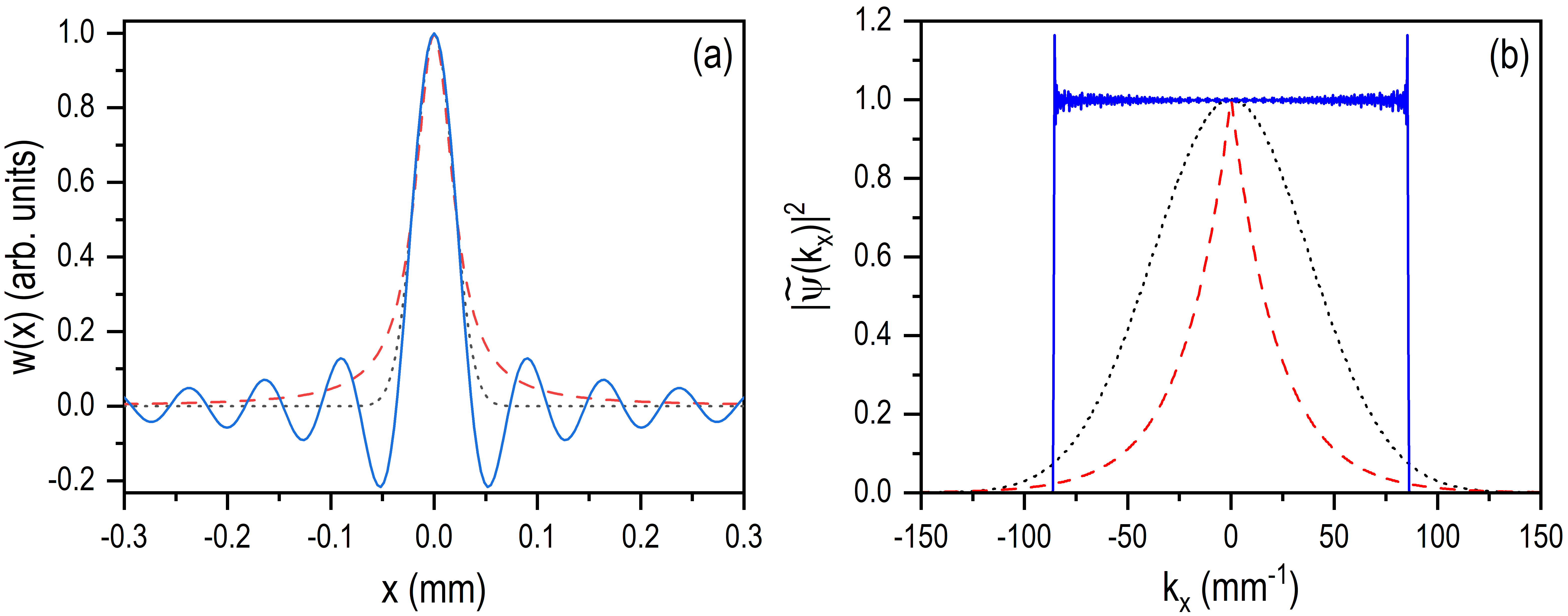
Figure 1: (a) Spatial dependence of the three aperture functions considered here, all with the same FWHM, $44.13$ $\mu$m. The Gaussian aperture function is represented with black dotted line, the Lorentzian aperture function with red dashed line, and the sinc-type aperture function with blue solid line. For a better comparison, the three functions are normalized to the unity. (b) Transverse power spectrum, $|\tilde{\psi}(k_{x})|^{2}$, of the input convoluted wave functions arising after applying the convolution with the aperture functions displayed in part (a) [type and color lines are in correspondence with the respective figures in (a)]. Again, for a better comparison, the three spectra have been normalized to the unity at their center.

The three aperture functions are shown in Fig. 1a, all with the same FWHM, $44.13$ $\mu$m, which is nearly half the FWHM of the leading maximum of the ideal (infinite energy) Airy beam considered, $96.13$ $\mu$m. For a better comparison, the three functions are plotted without the constant prefactor, so that their maxima coincide with 1, while they asymptotically approach 0 at large $x$. We notice that, although the three cases present nearly the same trend around $x_{c}$, the spatial extent of the sinc-type function is larger than in the other two cases. Nonetheless, if we inspect the transverse power spectrum, $|\tilde{\psi}(k_{x})|^{2}$, corresponding to the initial ansätze constructed with these aperture functions (see Fig. 1b), we notice that the three cases essentially span the same range of momenta, even though the profile of the respective spectra looks very different (again, for a better comparison, the three spectra have been normalized to the unity at their center). Given that the power spectrum of an ideal Airy beam is flat, with an infinite extension, we note that, while the Gaussian and Lorentzian aperture functions are going to introduce a gradually decreasing of the amplitude components involved in the Airy beam, the sinc-type aperture function, on the contrary, is going to essentially preserve the same amplitude for the spectral range spanned. In the current case, as it can be seen in Fig. 1b, this spectral range is $\Delta k_{x}=2/w_{s}\approx 171.76$ mm^-1, with all components, low and large spatial frequencies, essentially contributing the same. This is in sharp contrast with the other two aperture functions, where the low spatial frequencies will play a more prominent role than the large ones (more remarkable in the Lorentzian case than in the Gaussian one).

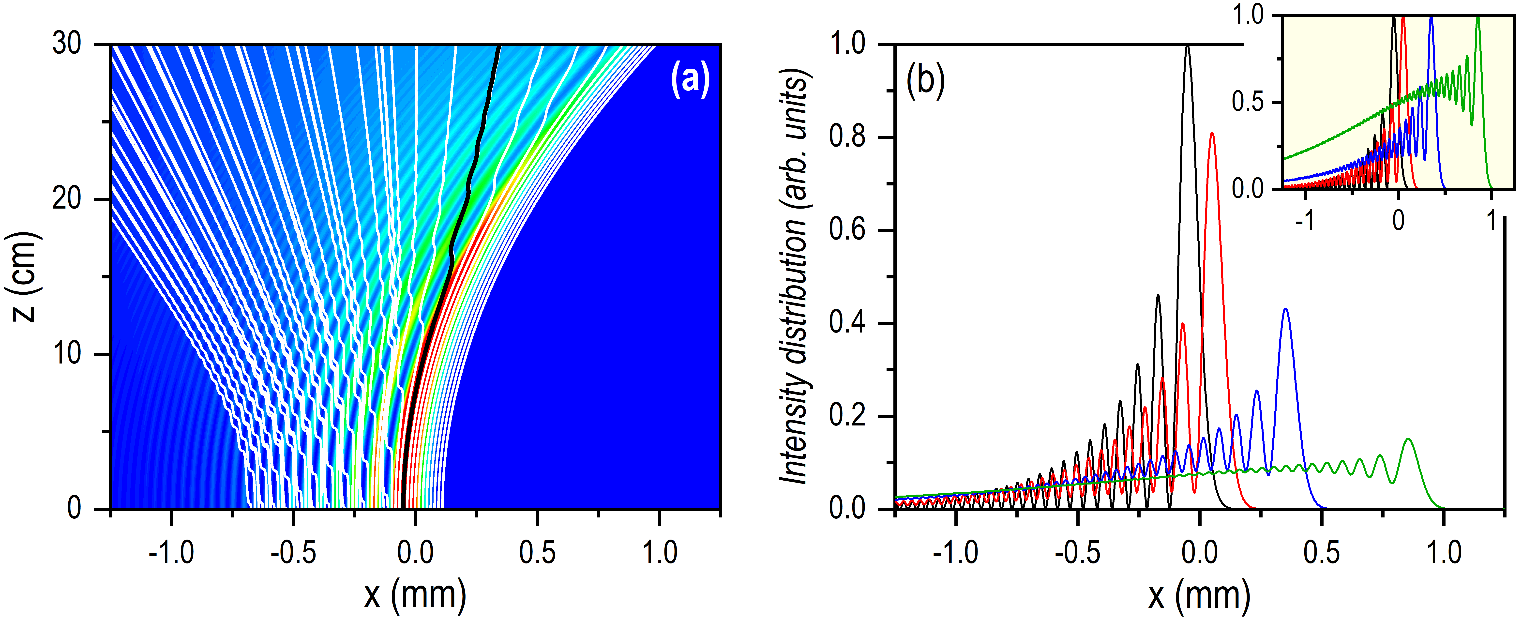
Figure 2: (a) Flux trajectories (white solid lines) associated with an Airy beam convoluted with a Gaussian aperture function. The initial conditions cover homogeneous the range spanned by the first foremost 10 maxima (including the leading one). The thick black line denotes a trajectory with its initial condition at the same position where the main maximum lies. (b) Profiles of the intensity distribution at: $z=0$ (black solid line), $z=10$ cm (red solid line), $z=20$ cm (blue solid line), and $z=30$ cm (green solid line). The curves have been normalized to unity taking into account the maximum value of the input beam (black solid line). In the inset, the same curves but each normalized to unity with respect to their corresponding maxima.

3 Results

3.1 Numerical dynamical simulations

To check the feasibility of the aperture functions here proposed, we have conducted a series of numerical simulations due to the non-analiticity of the propagation process in the three cases. As it is mentioned above, the parameter values considered are analogous to those used in the original experiments [4], which enables a more direct comparison with such experiments. Accordingly, in Figs. 2, 3, and 4 we show both an overall view of the propagation process in terms of trajectories superimposed on the corresponding density plots of the intensity distribution (see part a in these figures), and a series of snapshots of the intensity distribution at given values of $z$, which allow us to elucidate in a qualitative manner how fast the properties of ideal Airy beams are gradually lost (see part b in the figures).

In Fig. 2a we observe the propagation for a beam obtained with the Gaussian aperture function. As it is seen from the density plot, the beam behaves similarly to an ideal Airy beam for a relatively long distance, with a well-defined main leading maximum surviving up to nearly the largest $z$-value considered ($z=30$ cm). The snapshots displayed in Fig. 2b show clear evidence of such a behavior, particularly in the inset in this figure, where we have renormalized the three distribution for a better comparison. Nonetheless, unlike an ideal Airy beam, there is a progressive decrease in the intensity as well as a loss of the characteristics oscillations that form the tail of the beam. To understand this behavior, we resort to the trajectory description (see Fig. 2a). Accordingly, we note that, as it was mentioned in [13], the limited extension of the tail releases the beam from the infinite energy influx coming from the back. Consequently, not only the beam propagates forward, but it can also get diffracted backwards, which is what the trajectories (white solid lines) clearly show. Actually, we can observe that, if we choose an initial condition at the position of the maximum of the main peak of the initial beam, the corresponding trajectory (black solid line) start deviating from a parabolic-type curve for distances beyond $z=15$ cm, approximately. In other words, typical Airy beam properties are warranted for about $15$ cm; afterwards, the beam starts getting distorted.

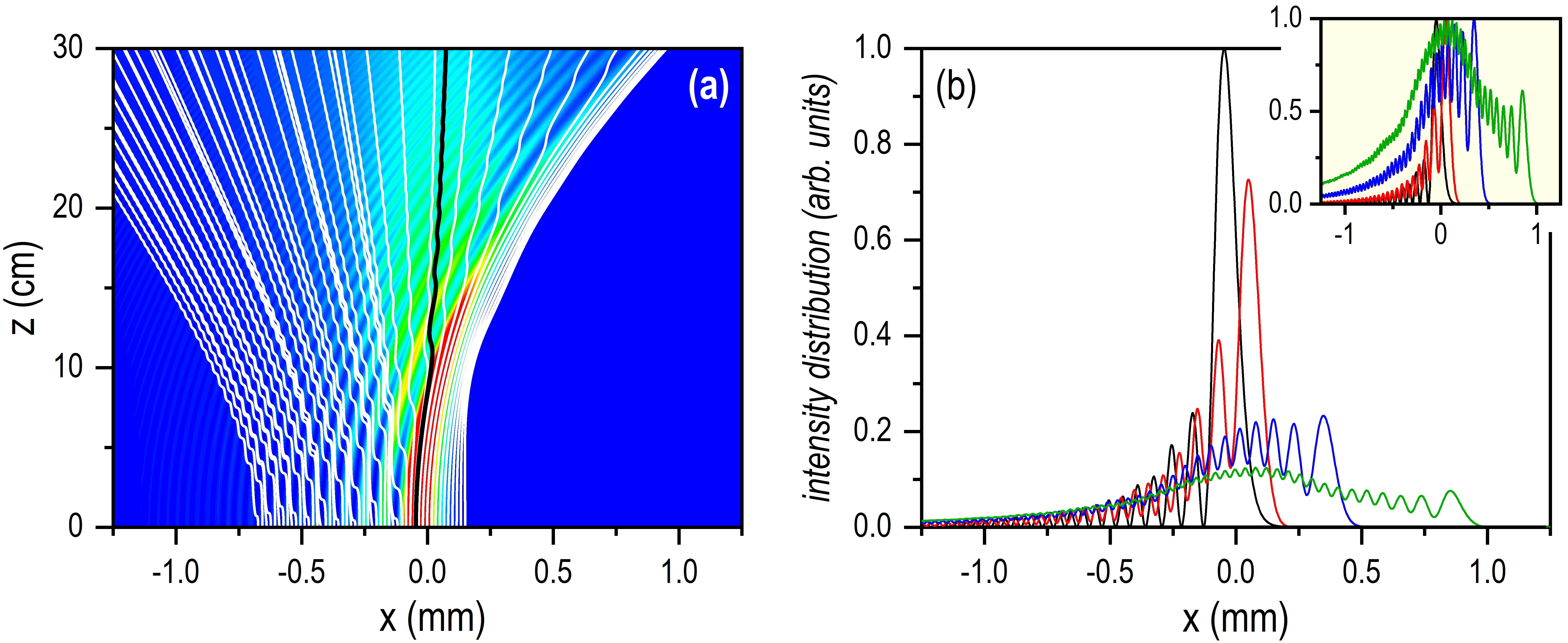
Figure 3: (a) Flux trajectories (white solid lines) associated with an Airy beam convoluted with a Lorentzian aperture function. The initial conditions cover homogeneous the range spanned by the first foremost 10 maxima (including the leading one). The thick black line denotes a trajectory with its initial condition at the same position where the main maximum lies. (b) Profiles of the intensity distribution at: $z=0$ (black solid line), $z=10$ cm (red solid line), $z=20$ cm (blue solid line), and $z=30$ cm (green solid line). The curves have been normalized to unity taking into account the maximum value of the input beam (black solid line). In the inset, the same curves but each normalized to unity with respect to their corresponding maxima.

The results for the Lorentzian aperture function are shown in Fig. 3. In this case, we observe a faster degradation, at shorter distances (around $10$ cm). In Fig. 3a the density plot reveals a large transfer of flux from the main peak to the rear secondary maxima, although with the seemingly net effect of getting stacked around $x=0$ mm. If we inspect Fig. 3b, effectively we clearly notice an accumulation of intensity around $x=0$ mm (see also inset), decreasing towards larger values of $x$. From the trajectory description, we find an overall picture that resembles that of the Gaussian aperture, but with the subtle difference that now the trajectory starting at the position of the main maximum remains nearly around the same position, without following the foremost ensemble of trajectories that still show a parabolic-type shape.

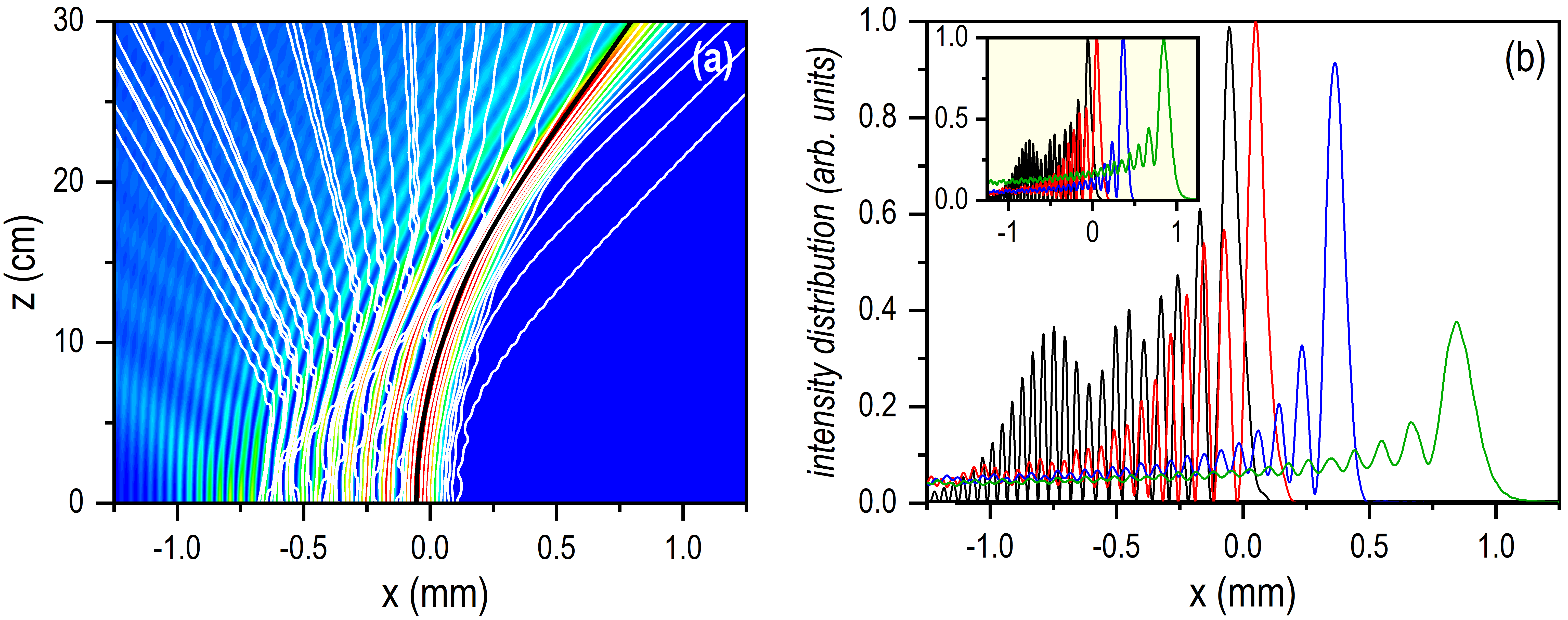
Figure 4: (a) Flux trajectories (white solid lines) associated with an Airy beam convoluted with a sinc-type aperture function. The initial conditions cover homogeneous the range spanned by the first foremost 10 maxima (including the leading one). The thick black line denotes a trajectory with its initial condition at the same position where the main maximum lies. (b) Profiles of the intensity distribution at: $z=0$ (black solid line), $z=10$ cm (red solid line), $z=20$ cm (blue solid line), and $z=30$ cm (green solid line). The curves have been normalized to unity taking into account the maximum value of the beam at $z=10$ cm (red solid line). In the inset, the same curves but each normalized to unity with respect to their corresponding maxima.

The two previous cases can be understood in the light of the strong filtering produced by the aperture functions considered in each case, which remove dramatically the high frequencies from the spectrum (see Fig. 1a). In sharp contrast, the case of the sinc-type aperture function, represented in Fig. 4, shows a very different picture. First, except from some intensity bursts propagating backwards, the density plot shows that all maxima, both the main peak and the secondary maxima, exhibit the typical parabolic shape expected for an Airy beam. The results in Fig. 4b clearly indicate that, effectively, the beam behaves like an ideal Airy beam for longer distances. On the other hand, the behavior of the trajectories also reveals that there is a larger survival of the parabolic shape for longer distances. Unlike the two previous cases, note that here the trajectories show a back and forth displacement, which keeps confined along parabolic-like channels for longer distances, until the backward energy influx reduces and they can escape (backwards). This behavior makes that a large portion of the foremost trajectories will keep showing their parabolic shape for rather long $z$-distances. Indeed, note that the trajectory started at the position of maximum of the main peak is nearly parabolic for the full propagation.

3.2 Dynamics of the main maximum

Apart from a local description of the propagation process, the trajectories also render interesting information that cannot be directly obtained from the density plots. In particular, to further understand physically the performance of the three aperture functions, we can investigate the local dynamics associated with a piece of the beam without perturbing its propagation. As it is inferred from [23], the intensity content within two any initial conditions will remain constant along $z$ provided we propagate those conditions along the corresponding trajectories. That is, if we consider two initial conditions delimiting a given intensity maximum (for instance, setting such initial conditions near the adjacent nodes, but not on top of them), we can determine at any subsequent $z$-value how the corresponding intensity distributes and within which boundaries.

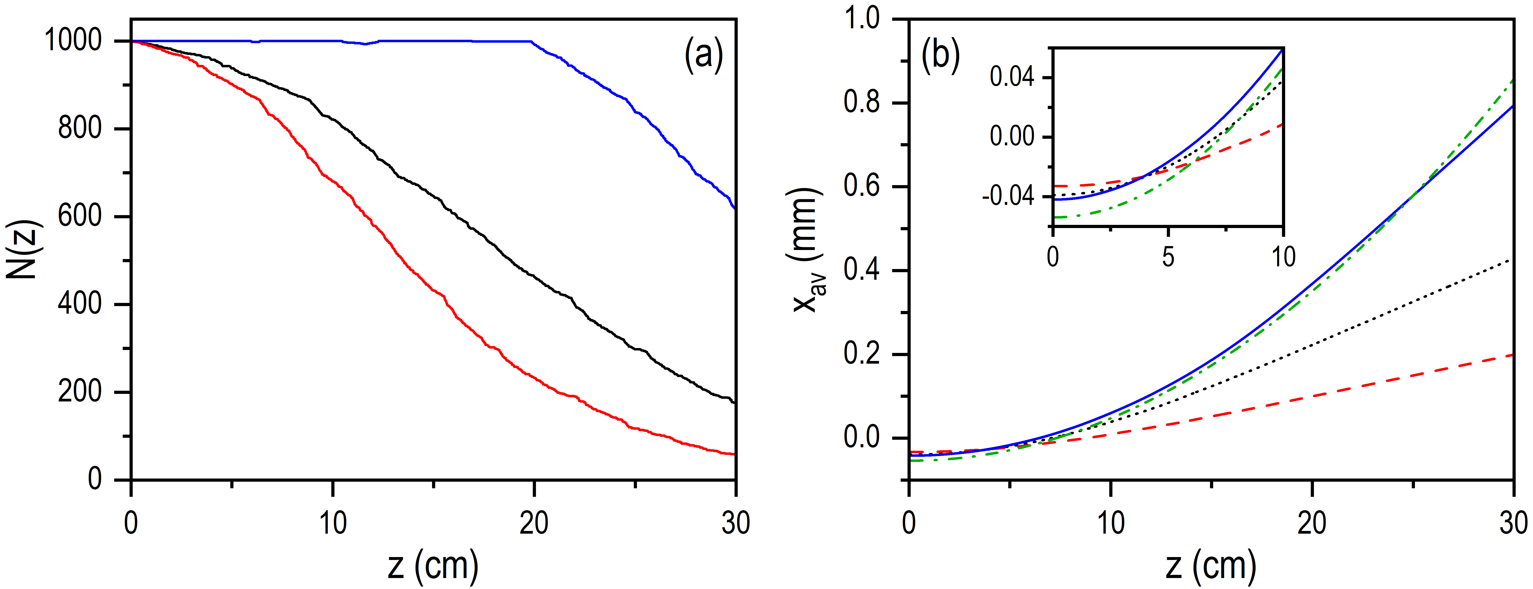
Figure 5: (a) Escape rate, $N(z)$, as a function of $z$ for the three aperture functions here considered. (b) Average position, $x_{\rm av}(z)$, over a sampling of 1,000 flux trajectories randomly distributed, at $z=0$, within the area covered by the leading maximum for the three aperture functions. The distribution of initial conditions have been taken according to a biGaussian distribution (see Appendix A). To compare with, the $z$-dependence of the leading maximum of an ideal (infinite energy) Airy beam is also shown, represented with green dashed line.

Accordingly, we have considered pairs of initial conditions between which we collect most of the intensity associated with the main peaks in the three cases (the ranges are given in Table 1 in Appendix A). Then, in order to understand how fast the corresponding beams deviate from an ideal Airy beam, we have computed two quantities. On the one hand, we have computed the escape rate, $N(z)$, which measures, along $z$, the intensity confined within two boundaries given by two parabolic trajectories. It is clear that the better the preservation of the ideal Airy beam properties the larger the value of $N(z)$ for larger and larger $z$-values. This quantity is plotted in Fig. 5a. As it can be seen, the decay of $N(z)$ is relatively fast for the Gaussian and the Lorentzian aperture functions, although the falloff for the latter is still slightly larger. While the energy (proportional to the number of trajectories) decays to about a half at $z\approx 18.8$ cm for the Gaussian aperture function, in the Lorentizan case the same takes place at $z\approx 13.5$ cm. This corresponds to the degradation of the intensity distribution profile observed in Figs. 2a and 3a, respectively. On the contrary, for the sinc-type aperture function, $N(z)$ remains nearly constant until $z\approx 19.8$ cm and, extrapolating data, a decrease to about $50\%$ is only expected for larger distances ($z\approx 33.5$ cm), which is in correspondence with the behavior observed in Fig. 4a.

On the other hand, taking into account that those initial conditions have been randomly distributed according to the intensity distribution, their average, $x_{av}$, can provide an objective measure of the self-accelerated propagation of only this beam. Again, the better the preservation of the ideal behavior, the closer this average will be to a parabola. This quantity is represented in Fig. 5b (see solid lines), where we have also included the trajectories associated with the initial condition taken at the position of the maximum of the respective main peaks (dashed lines). To compare with, we have also included the trajectory of an ideal Airy beam with its initial position at the $x$-value where the main peak of such a beam reaches its maximum (see green dotted line). As we can see, the trajectories corresponding to the maximum in the Gaussian and Lorentzian cases start deviating from the average value at short and medium distances, respectively, in agreement with what we already saw in Figs. 2 and 3. More specifically, such a deviation starts being remarkable at about $20$ cm for the Gaussian aperture function, and about $10$ cm for the Lorentzian one. These distances can be used as distinctive objective criterion to determine when the performance of the corresponding aperture function becomes poor. In therms of the average, $x_{av}$, this loss of efficiency is indicated by the transition from a nearly parabolic behavior, at the initial stages of the propagation, to a seemingly linear behavior at larger distances, which is produced by the gradual drain of trajectories (flux) backwards.

In the case of the sinc-type aperture function, again we observe a very different behavior, since both the average and the trajectory of the maximum basically propagate parallel one another. More interestingly, these two quantities overlap in a good approximation the trajectory of the maximum for an ideal Airy beam; only at large $z$-values we start observing a discrepancy, which is a signature of the loss of the ideal behavior.

4 Discussion

We have introduced a trajectory-based methodology to investigate the effect of limiting the energy content of Airy beams by means of aperture functions with different shapes, and hence to elucidate which functional form better preserves the properties of an ideal Airy beam at the input. Thus, we have combined conventional propagation simulations, to determine the intensity distribution at difference distances from the input plane, with the above mentioned non-conventional approach based on an on-the-fly computation of the transverse energy flux, which provides us with information at a more local level. The transverse energy flux, described in terms of sets of trajectories, enables a description and analysis of the propagation process on a single-event basis, making more intuitive the properties of Airy beams (shape invariance and self-accelerated propagation) at the same time that it is also possible to perform some additional quantitative analyses of specific features.

From our analysis, we conclude that, among the three types of aperture functions investigated, sinc-type ones show a better performance, because they basically introduce a cut in the beam spectrum, without modifying the amplitude of its components, unlike other types of aperture functions, such as Gaussian or Lorentzian profiles. The trajectories show a very interesting picture in this regard. On the one hand, we note that the trajectories associated with the Gaussian or the Lorentzian aperture functions make evident a monotonous energy dissipation backwards. This continuous flow produces a rather fast lost of fringe visibility of the intensity distribution, as it is manifested by the corresponding escape rates, and hence the also fast loss of the typical properties of an Airy beam at relatively close distances from the input plane. In particular, it has been noticed that the self-accelerated displacement that should undergo the average position of the energy accumulated in the main maximum is gradually lost.

On the other, in the case of the sinc-type aperture function, the fact that all spatial spectral components play have nearly the same amplitude provokes that the presence of a wiggling displacement of the trajectories and hence a back-and-forth energy flow between adjacent intensity maxima. This oscillatory behavior enables the preservation of the typical Airy beam features for much longer distances, even though the gradual degradation observed in the pattern along them. Furthermore, unlike the two previous cases, here it has been shown that the average position of the energy accumulated in the main maximum follows very nicely the behavior expected for an ideal Airy beam.

In sum, the present analysis is aimed at providing new insights into the behavior of finite-energy Airy beams, and therefore also expected to contribute to the design and development of novel applications exploiting finite-energy Airy beams. Moreover, it is also worth noting that, by virtue of the tight analogy between the paraxial Helmholtz equation and the Schrödinger equation, the results shown and discussed here are also directly transferable to the generation and exploitation of Airy beams with nonzero mass particles, as it is the case of electron Airy beams, first produced in 2013 by Voloch-Bloch et al. [24].

Appendix A Numerical and data analysis methods

The simulations conducted in this work to obtain the beam propagation and the corresponding trajectories, have been carried out following the same procedure formerly used in [13], based on the split-step for beam propagation and a spectral recast of the equation of motion for the trajectories [25]. For the trajectories shown in Figs. 2, 3, and 4, we have considered an evenly-spaced distribution of 50 initial conditions, taken from a range that covers the first 10 intensity maxima of the input beam (the leading maximum and the nine subsequent secondary maxima).

Concerning the random distribution required to compute the quantities shown in Fig. 5, first we have fitted the main maximum of the input intensity distributions (see black line curves in Figs. 2, 3, and 4) to the biGaussian distribution,

$$f(x)=\left\{\begin{array}[]{lcc}\exp[-(x-x_{0})^{2}/2\sigma_{l}^{2}],&&x<x_{0}\\ \exp[-(x-x_{0})^{2}/2\sigma_{r}^{2}],&&x\geq x_{0}\\ \end{array}\right.,$$ (33)

which captures fairly well the asymmetry of such a maximum. The values for the parameters $x_{0}$, $\sigma_{l}$, and $\sigma_{r}$ obtained from the corresponding fitting procedures for the three cases are given in Table 1.

Table 1: Parameters used in the fitting of the main maximum to a biGaussian distribution.

aperture function	$x_{c}$ (mm)	$w_{1}$ (mm)	$w_{2}$ (mm)	i.c. range (mm)
Gaussian	$-0.05688$	$0.02647$	$0.04844$	$(-0.123,0.115)$
Lorentzian	$-0.05363$	$0.02887$	$0.05412$	$(-0.128,0.161)$
sinc-type	$-0.06016$	$0.02341$	$0.04536$	$(-0.124,0.112)$

Regarding the specific random choice, first, we select randomly from a $[0,1)$ uniform distribution a number. If this number is smaller than the ratio $\sigma_{l}/(\sigma_{l}+\sigma_{r})$, then we associate the initial condition to the left side of the biGaussian distribution (i.e., $x<x_{0}$); otherwise, the initial condition is associated with the right side. A number is then picked up randomly following a Gaussian distribution centered at $x_{0}$ and with a width $\sigma_{l}$, if the previous choice laid on the left side of the distribution, or $\sigma_{r}$, if the choice led to the right side. It might happen that the number obtained from this procedure will lay on the opposite side where it is supposed to be; in such a case, the algorithm re-start the choice of the side and repeats the process.

Funding

Agencia Estatal de Investigación (PID2019-104268GB-C21, PID2021-127781NB-I00, RED2022-134391-T).

Disclosures

The authors declare no conflicts of interest.

Data Availability

Data underlying the results presented in this paper are not publicly available, but may be obtained from the authors upon reasonable request.

References

- [1] M. V. Berry and N. L. Balazs, “Nonspreading wave packets,” \JournalTitleAm. J. Phys. 47, 264–267 (1979).
- [2] D. M. Greenberger, “Comment on “Nonspreading wave packets”,” \JournalTitleAm. J. Phys. 48, 256–256 (1980).
- [3] K. Unnikrishnan and A. R. P. Rau, “Uniqueness of the Airy packet in quantum mechanics,” \JournalTitleAm. J. Phys. 64, 1034–1035 (1996).
- [4] G. A. Siviloglou, J. Broky, A. Dogariu, and D. N. Christodoulides, “Observation of accelerating Airy beams,” \JournalTitlePhys. Rev. Lett. 99, 213901 (2007).
- [5] A. Forbes, M. de Oliveira, and M. R. Dennis, “Structured light,” \JournalTitleNat. Photonics 15, 253–262 (2021).
- [6] J. Wang and Y. Liang, “Generation and detection of structured light: A review,” \JournalTitleFront. Phys. 9, 688284 (2021).
- [7] Y. Zhang, H. Zhong, M. R. Belić, and Y. Zhang, “Guided self-accelerating Airy beams—-A mini-review,” \JournalTitleAppl. Sci. 7 (2017).
- [8] N. K. Efremidis, Z. Chen, M. Segev, and D. N. Christodoulides, “Airy beams and accelerating waves: An overview of recent advances,” \JournalTitleOptica 6, 686–701 (2019).
- [9] G. A. Siviloglou and D. N. Christodoulides, “Accelerating finite energy Airy beams,” \JournalTitleOpt. Lett. 32, 979–981 (2007).
- [10] Y. Zhang, M. R. Belić, L. Zhang, W. Zhong, D. Zhu, R. Wang, and Y. Zhang, “Periodic inversion and phase transition of finite energy Airy beams in a medium with parabolic potential,” \JournalTitleOpt. Express 23, 10467–10480 (2015).
- [11] F. Liu, J. Zhang, W.-P. Zhong, M. R. Belić, Y. Zhang, Y. Zhang, F. Li, and Y. Zhang, “Manipulation of Airy beams in dynamic parabolic potentials,” \JournalTitleAnnalen der Physik 532, 1900584 (2020).
- [12] D. Xu, Y. Liu, Z. Mo, J. Jiang, J. Shi, Z. Liang, Y. Wu, J. Zhao, H. Yang, H. Huang, H. Liu, L. Shui, and D. Deng, “Shaping autofocusing Airy beams through the modification of Fourier spectrum,” \JournalTitleOpt. Express 30, 232–242 (2022).
- [13] A. S. Sanz, “Flux trajectory analysis of Airy-type beams,” \JournalTitleJ. Opt. Soc. Am. A 39, C79–C85 (2022).
- [14] H. Margenau and G. M. Murphy, The Mathematics of Physics and Chemistry (D. Van Nostrand, Princeton, NJ, 1943).
- [15] A. S. Sanz and S. Miret-Artés, A Trajectory Description of Quantum Processes. I. Fundamentals, vol. 850 of Lecture Notes in Physics (Springer, Berlin, 2012).
- [16] L. Allen, M. W. Beijersbergen, R. J. C. Spreeuw, and J. P. Woerdman, “Orbital angular momentum of light and the transformation of Laguerre-Gaussian laser modes,” \JournalTitlePhys. Rev. A 45, 8185–8189 (1992).
- [17] J. Broky, G. A. Siviloglou, A. Dogariu, and D. N. Christodoulides, “Self-healing properties of optical Airy beams,” \JournalTitleOpt. Express 16, 12880–12891 (2008).
- [18] A. S. Sanz, J. Campos-Martínez, and S. Miret-Artés, “Transmission properties in waveguides: An optical streamline analysis,” \JournalTitleJ. Opt. Am. Soc. A 29, 695–701 (2012).
- [19] A. S. Sanz, M. Davidović, and M. Božić, “Bohmian-based approach to Gauss-Maxwell beams,” \JournalTitleAppl. Sci. 10, 1808(1–25) (2020).
- [20] A. S. Sanz, L. L. Sanchez-Soto, and A. Aiello, “A quantum trajectory analysis of singular wave functions,” (2023).
- [21] A. S. Sanz and S. Miret-Artés, “On the unique mapping relationship between initial and final quantum states,” \JournalTitleAnn. Phys. 339, 11–21 (2013).
- [22] A. García-Sánchez and A. S. Sanz, “Analysis of the gradual transition from the near to the far field in single-slit diffraction,” \JournalTitlePhys. Scr. 97, 055507 (2022).
- [23] A. S. Sanz and S. Miret-Artés, “Setting-up tunneling conditions by means of Bohmian mechanics,” \JournalTitleJ. Phys. A: Math. Theor. 44, 485301(1–17) (2011).
- [24] N. Voloch-Bloch, Y. Lereah, Y. Lilach, A. Gover, and A. Arie, “Generation of electron Airy beams,” \JournalTitleNature 494, 331–335 (2013).
- [25] A. S. Sanz and S. Miret-Artés, A Trajectory Description of Quantum Processes. II. Applications, vol. 831 of Lecture Notes in Physics (Springer, Berlin, 2014).