T(w)o patch or not t(w)o patch: A novel additional food model

Abstract.

A number of top down bio-control models have been proposed where the predators’ efficacy is enhanced via the provision of additional food (AF) [39, 43, 42]. These can lead to infinite time blow-up of the predator [25]. Predator interference, predator competition, refuge, pest defense and cannibalism have been proposed to achieve pest extinction, while keeping the predator population bounded, but entail quadratic or higher order damping terms. Thus an AF model with monotone pest dependent functional response, devoid of these mechanisms, cannot yield the pest extinction state.

In the current manuscript we propose a novel patch driven bio-control model, with monotone pest dependent functional response. Here a predator is introduced into a “patch” such as a prairie strip with AF, and then disperses into a neighboring “patch” such as a crop field, to target a pest. Assuming only linear dispersal in the predator, we show, (i) blow-up in the predator can be prevented in both the prairie strip and the crop field, (ii) the pest extinction state is attainable in the crop field, (iii) the AF model with patch structure can keep pest densities lower than the AF model without patch structure and/or the classical top-down bio-control model, (iv) the AF model with patch structure possesses rich dynamics including chaos. In particular, one observes “patch specific chaos” - the pest occupying the crop-field can oscillate chaotically, while the pest in the prairie strip oscillates periodically. We discuss these results in light of bio-control strategies that would utilize prairie strips.

Urvashi Verma¹, Aniket Banerjee¹ and Rana D. Parshad¹

1) Department of Mathematics,

Iowa State University,

Ames, IA 50011, USA.

1. Introduction

Invasive/pest species continue to be a significant global problem [28, 23, 35], of immense scale. Pests such as the European corn borer, Western corn root worm and Soybean Aphid cause damages to crop yield in the United States in excess of $\$$ 3 billion annually [32, 22, 2]. Populations of the invasive cane toad in Western Australia, are reaching explosive levels [46], despite several intervention strategies, while the burmese python invasion in the everglades region of south Florida, has caused an excessive drop in local prey populations [9]. Thus the control of invasive species is crucial, but also challenging [35]. Typical control methods use chemical pesticides, despite negative environmental impacts, [27]. A self sustaining and environmentally friendly alternative is classical or top down bio-control. This is the introduction of natural enemies/predators of the pest species [47, 38], that will in turn depredate on the pest. Bio-control comes with associated risks [31]. These include non-target effects, [26], which could lead to uncontrolled growth of the predator population. This has been seen with the cane toad in Western Australia, and the burmese python in south Florida [46, 9]. In order to help support bio-control programs several innovative invasion control strategies using niche theory, and competition theory have been proposed [13, 4]. For example, lowering nitrogen levels in soil via microbe use, has been used as a management strategy, to enhance intraspecies competition among native plants, and preempt invasions [48]. Among these, is also the method of Additional/Alternative food (AF). Herein the efficacy of the predator can be “boosted” by supplementing it with an AF source [31, 44]. A number of mathematical models that describe predator pest dynamics with AF have been developed, [41, 40, 29, 39, 43, 42, 1]. These works posit that if high quality additional food is provided to the introduced predator in sufficient quantity then pest extinction is achieved.

Although there is a large body of work on AF mediated bio-control, AF models with dispersal (both explicit or implicit) have been far less investigated. Dispersal, both as a phenomenon and as a strategy is much studied in ecology [21, 8]. Species disperse in search of prey, mates and better habitat [5], and they will often disperse between small interactive spatial components or “patches”. To this end, patch models have been intensely investigated [50, 45]. Interestingly, the dynamics that one sees in the classic mean field sense, in predator-prey or competitive scenarios (where there is essentially one large patch) may not be true in the two (or multi) patch setting, with dispersal between these patches [11, 3]. There is also a growing body of evidence for this from landscape ecology. In particular, there is large evidence that natural enemies of pests are many times more abundant in smaller patches surrounding crop fields, and can depend on connectivity of crop fields to non-crop habitats [12], furthermore multitrophic diversity can be facilitated by increasing crop heterogeneity as well [10, 36]. From a pragmatic viewpoint, the utilisation of these theoretical results to achieve target control scenarios of species, requires the management of such landscapes. This is crucial for improved ecosystem structure and function, and so is also a well studied area in ecology [15].

Among these landscape management practices are several innovative strategies, including the planting of prairie strips. These are a conservation practice to protects soil and water while providing suitable habitat for wildlife. These enable increased productivity which leads to higher crop yields, reduce sediment movement, and maintain high phosphorus and nitrogen levels. All in all this is a high value practice in agriculture [34]. Among such practice, more recent innovation has led to programs such as STRIPS (Science-based Trails of Row crops Integrated with Prairie Strips) in the mid-western US. This has been pioneered and led by the state of Iowa, in particular [33]. The row crops as earlier mentioned, provide a suitable habitat for several species, and enhance biodiversity and ecosystem function. In particular, these could include better habitat for bio-control agents such as predators that would disperse into the adjacent crop fields to target pests. However, to the best of our knowledge an AF driven bio-control model, where a predator is housed or introduced into a prairie strip (or a STRIP), where it is provided with AF, and then subsequently disperses into a neighboring crop field to target a pest, has not been investigated. The current manuscript is a first attempt in this direction.

2. Prior Results

2.1. General Predator-Pest Model

The following general model for an introduced predator population $y(t)$ depredating on a target pest population $x(t)$, while also provided with an additional food source of quality $\frac{1}{\alpha}$ and quantity $\xi$, has been proposed in the literature,

(2.1) $$\frac{dx}{dt}=x\left(1-\frac{x}{\gamma}\right)-f(x,\xi,\alpha)y,\ \frac{dy}{dt}=g(x,\xi,\alpha)y-\delta y.$$

Here $f(x,\xi,\alpha)$ is the functional response of the predator, that is pest dependent but also dependent on the additional food (hence the explicit dependence on $\xi,\alpha$). Likewise, $g(x,\xi,\alpha)$ is the numerical response of the predator. If $\xi=0$, that is there is no additional food, the model reduces to a classical predator-prey model of Gause type, that is $f(x,0,0)=g(x,0,0)$, where $f$ has the standard properties of a functional response. For these models we know pest eradication is not possible, as the only pest free state is $(0,0)$, which is typically unstable [14]. Thus modeling the dynamics of an introduced predator and its prey, a targeted pest via this approach, where the constructed $f(x,\xi,\alpha),g(x,\xi,\alpha)$ are used as a means to achieve a pest free state, has both practical and theoretical value, and thus has been well studied. Table 1, summarizes some of the key literature, in terms of the functional forms used in these models.

Table 1. Dynamics of predator-pest models supplemented with AF

	Functional form	Relevant literature	AF requirement	Effect on pest control
(i)	$f(x,\xi,\alpha)=\frac{x}{1+\alpha\xi+x}$	[41, 40, 39]	$\xi>\frac{\delta}{\beta-\delta\alpha}$	Pest is eradicated, switching AF
	$g(x,\xi,\alpha)=\frac{\beta(x+\xi)}{1+\alpha\xi+x}$			maintains/eliminates predator
(ii)	$f(x,\xi,\alpha)=\frac{x^{2}}{1+\alpha\xi^{2}+x^{2}}$	[43]	$\xi>\sqrt{\frac{\delta}{\beta-\delta\alpha}}$	Pest is eradicated, switching AF
	$g(x,\xi,\alpha)=\frac{\beta(x^{2}+\xi^{2})}{1+\alpha\xi^{2}+x^{2}}$			maintains/eliminates predator
(iii)	$f(x,\xi,\alpha)=\frac{x}{(1+\alpha\xi)(\omega x^{2}+1)+x}$	[42]	$\xi>\frac{\delta}{\beta-\delta\alpha}$	Pest is eradicated, switching AF
	$g(x,\xi,\alpha)=\frac{\beta(x+\xi(\omega x^{2}+1)}{(1+\alpha\xi)(\omega x^{2}+1)+x}$			maintains/eliminates predator
(iv)	$f(x,\xi,\alpha)=\frac{x}{1+\alpha\xi+x+\epsilon y}$	[29]	$\beta\xi=\delta(1+\alpha)$	Pest extinction state stabilises,
	$g(x,\xi,\alpha)=\frac{\beta(x+\xi)}{1+\alpha\xi+x+\epsilon y}$		$\beta(\gamma+\xi)=\delta(1+\alpha\xi+\gamma)$	via TC

The effect of increasing the quantity of AF $\xi$ herein is to push the vertical predator nullcline to the left, thereby decreasing the equilibrium pest level. The extinction mechanism works by inputting $\xi>\xi_{critical}$ (Here $\xi_{critical}$ depends on the model parameters, and changes from model to model) s.t. the predator nullcline is pushed left past the y-axis (predator axis), into the $2^{nd}$ quadrant, annihilating any positive interior equilibrium. Via the positivity of solutions, trajectories will converge onto the predator axis, yielding pest extinction. Furthermore, this can be done in minimal time [40, 39, 1].

We focus on the case with type II response next.

2.2. Type II response

The basic predator-pest model, with type II response is as follows,

(2.2) $$\frac{dx}{dt}=x\left(1-\frac{x}{\gamma}\right)-\frac{xy}{1+\alpha\xi+x},\ \frac{dy}{dt}=\frac{\beta xy}{1+\alpha\xi+x}+\frac{\beta\xi y}{1+\alpha\xi+x}-\delta y.$$

We recap the key results from the literature. These are essentially categorized based on quality and quantity of additional food. We will focus on the case of “high quality” additional food, that is if $\frac{1}{\alpha}>\frac{\delta}{\beta}\Leftrightarrow\beta-\delta\alpha>0$. Two regimes of the quantity of additional food are possible, detailed next.

2.2.1. The small additional food regime

We first consider $\xi\in(0,\frac{\delta}{\beta-\delta\alpha})$, the “small” additional food regime. We further assume $\beta-\delta>0$, this is biologically realistic, and follows from standard theory when $\xi=0$, and (2.2) reduces to the standard Rosenzweig McArthur model [14]. In this case, there is one interior equilibrium which is stable if, $\frac{\delta}{\beta-\delta}<\gamma\leq\frac{\beta+\delta}{\beta-\delta}$, and predator and pest co-exist. Or, the equilibrium could be unstable, with the existence of a stable limit cycle, if $\frac{\delta}{\beta-\delta}\leq\frac{\beta+\delta}{\beta-\delta}<\gamma$. That is a Hopf Bifurcation occurs at $\frac{\beta+\delta}{\beta-\delta}=\gamma$. In this case the predator and pest would now exhibit cyclical dynamics [41]. Increasing additional food in the interval $(0,\frac{\delta}{\beta-\delta\alpha}]$, lowers pest equilibrium (as essentially this moves the vertical predator nullcline closer and closer to the y-axis). However, the pest cannot be driven extinct for any $\xi\in(0,\frac{\delta}{\beta-\delta\alpha})$.

2.2.2. The large additional food regime

The literature [41, 39, 40] claimed that increasing the additional food supply beyond this interval, so if $\xi\in\left(\frac{\delta}{\beta-\delta\alpha},\infty\right)$, eradicates the pest from the ecosystem in a finite time, and from that time the predators survive only on the additional food supply. We recap the result of interest from the literature [41, 39], which quantifies the efficacy of the predator to achieve pest eradication when supplemented with additional food via (2.2),

Lemma 1.

Consider the predator-pest system described via (2.2). If the quality of the additional food satisfies $\beta-\delta\alpha>0$, then the pest can be eradicated from the ecosystem in a finite time by providing the predator with additional food of quantity $\xi>\frac{\delta}{\beta-\delta\alpha}$.

However, we recap the following [Theorem 2.2, [24]],

Theorem 1.

Consider the predator-pest system described via (2.2). Pest eradication is not possible in finite time even if the quality of the additional food satisfies $\beta-\delta\alpha>0$ and the quantity of the additional food satisfies $\xi>\frac{\delta}{\beta-\delta\alpha}$.

Note, if $\xi>\frac{\delta}{\beta-\delta\alpha}$, the dynamics of (2.2) always result in blow-up in infinite time of the predator density. In [25] we show,

Theorem 2.

Consider the predator-pest system described via (2.2), and assume the parametric restrictions, $\beta-\delta\alpha>0$. If the quantity of additional food $\xi$ is chosen s.t., $\xi\in\left(\frac{\delta}{\beta-\delta\alpha},\infty\right)$, then solutions initiating from any positive initial condition, blow up in infinite time. That is,

$$\lim_{t\rightarrow\infty}{(x(t),y(t))}\rightarrow(0,\infty)$$

2.3. Type III response

The type III response has been considered in a number of AF models, [43, 42]. However an adaptation of theorem 2 enables the following corollary,

Corollary 1.

Consider a predator-pest system described via (2.1), where $f(x,\xi,\alpha)=\frac{x^{2}}{1+\alpha\xi^{2}+x^{2}},g(x,\xi,\alpha)=\frac{\beta(x^{2}+\xi^{2})}{1+\alpha\xi^{2}+x^{2}}$ and assume the parametric restrictions, $\beta-\delta\alpha>0$. If the quantity of additional food $\xi$ is chosen s.t., $\xi\in\left(\sqrt{\frac{\delta}{\beta-\delta\alpha}},\infty\right)$, then solutions initiating from any positive initial condition, blow up in infinite time. That is,

$$\lim_{t\rightarrow\infty}{(x(t),y(t))}\rightarrow(0,\infty)$$

2.4. Predator dependent responses and the inhibitory effect

In order to prevent unbounded predator growth several alternative mechanisms have been proposed.

• The inhibitory effect produced by prey defense, such as via the type IV functional response [1].

• The inhibitory effects produced by predator interference, such as via the Beddington-Deangelis functional response [30, 49].

• The inhibitory effect produced by a purely ratio dependent response [17, 16].

• The damping effect produced by intraspecific predator competition [25].

All of the above prevent unbounded growth of the predator. In Prasad et al [30], the following model was proposed, (2.3).

(2.3) $$\frac{dx}{dt}=x\left(1-\frac{x}{k}\right)-\frac{xy}{1+\alpha\xi+x+\epsilon y},\ \frac{dy}{dt}=\frac{\beta(x+\xi)y}{1+\alpha\xi+x+\epsilon y}-\delta y$$

Herein, the Beddington–DeAngelis functional response [6] incorporates mutual interference amongst predators, via the term $\epsilon y$ where the parameter $\epsilon$ is a measure of this mutual interference effect. The analysis in [30] focused on two separate cases, (i) high interference $\epsilon>1$ (ii) low interference $0<\epsilon<1$. In (i) there is always one unique interior equilibrium - if a feasible pest free equilibrium exists it is a saddle. Thus from the point of view of pest eradication, high predator interference is not desirable. In that no matter what quality and/or quantity of additional food are chosen, the pest eradication state cannot be (even locally) attracting. In case (ii) it was shown therein that,

• The predator density is always bounded. It cannot grow past a uniform (in parameter) bound, no matter how the parameters are changed, so as to engineer control of the pest.

• There can exist one unique interior equilibrium, as long as $\xi<\frac{\delta}{\beta-\delta\alpha-\beta\epsilon}$.

• A pest-free equilibrium can coexist with the interior equilibrium - in that case, the pest-free equilibrium is always a saddle.

• The pest free state is globally stable if $\xi>\frac{\delta}{\beta-\delta\alpha-\beta\epsilon}$. This change of stability occurs through a transcritical bifurcation.

• A predator-free equilibrium can also exist.

The analysis in [30] is based on the geometric assumption that the slope of the predator nullcline (say $m_{1}$) in (2.3) is greater than the slope of the tangent line to the prey nullcline (say $m$) at $(0,\frac{1+\alpha\xi}{1-\epsilon})$, that is where it cuts the predator (y) axis. This is the reason that the authors in [30] derive global stability of the pest free state, when the condition in (iv) above holds. This condition follows by choosing the $y$-intercept of the predator nullcline to be large than where the prey nullcline intersects the $y$-axis. This in conjunction with $m_{1}>m$, yields global stability of the pest free state. Thus, the fundamental premise of [30], is to assume AF introductions $\xi$, such that $\xi>h(\epsilon)$. Note, recently we consider $\xi<h(\epsilon)$, and provide a much tighter window on the quantities of AF needed for pest eradication. In particular, we are able to derive pest extinction for $h(\epsilon)>f(\epsilon)>\xi>g(\epsilon)$, [49].

3. Additional Food Patch Model Formulation

We assume that our landscape is divided into two sub-units, a crop field which is the larger unit, and a prairie strip which is the smaller unit. These are the two patches that make up our landscape. We will refer to the prairie strip as $\Omega_{1}$ and the crop field as $\Omega_{2}$. We assume that the prairie strip by design possesses row crops that will provide alternative/additional food to an introduced predator, that would enhance its efficacy to target a pest species, that resides primarily in the crop field. The crop field has no AF.

Thus for the patch $\Omega_{1}$, we assume the quantity of AF as $\xi$ and the quality of AF as $\frac{1}{\alpha}$. Thus essentially in $\Omega_{1}$ we have an AF driven predator-pest system, for a pest density $x_{1}$ and a predator density $y_{1}$. We choose the classical Holling type II functional response, for the functional response of the pest. We assume the predators will disperse between $\Omega_{1}$ and $\Omega_{2}$, via linear dispersal. The net predator dispersal from $\Omega_{1}$ into $\Omega_{2}$ takes place at rate $k_{2}$. This is modeled as,

$$\boxed{\dot{x_{1}}=x_{1}\left(1-\frac{x_{1}}{k}\right)-\frac{x_{1}y_{1}}{1+x_{1}+\alpha\xi},\ \dot{y_{1}}=\epsilon_{1}\left(\frac{x_{1}+\xi}{1+x_{1}+\alpha\xi}\right)\ y_{1}-\delta_{1}y_{1}+k_{2}\left(y_{2}-y_{1}\right)}$$

In $\Omega_{2}$, since there is no AF, we have a classical predator-prey(pest) dynamics, for a pest density $x_{2}$ and a predator density $y_{2}$. The net predator dispersal from $\Omega_{2}$ into $\Omega_{1}$ takes place at rate $k_{4}$. Thus in $\Omega_{2}$ the dynamics are modeled as,

$$\boxed{\dot{x_{2}}=x_{2}\left(1-\frac{x_{2}}{k}\right)-\frac{x_{2}y_{2}}{1+x_{2}},\ \dot{y_{2}}=\epsilon_{2}\left(\frac{x_{2}}{1+x_{2}}\right)\ y_{2}-\delta_{2}y_{2}+k_{4}\left(y_{1}-y_{2}\right)}$$

We further assume that the pest does not move between the patches. That is, the pest prefers its primary host, the crop in the crop field, however, there could be some presence of the pest in the prairie strip, due to long range dispersal effects such as wind (not modeled herein) or the presence of certain row crops in the strip, as alternative hosts.

Coupling the above equations, leads to the following system,

(3.1) $$\dot{x_{1}} =x_{1}\left(1-\frac{x_{1}}{k}\right)-\frac{x_{1}y_{1}}{1+x_{1}+\alpha\xi}$$

$$\dot{y_{1}} =\epsilon_{1}\left(\frac{x_{1}+\xi}{1+x_{1}+\alpha\xi}\right)\ y_{1}-\delta_{1}y_{1}+k_{2}\left(y_{2}-y_{1}\right)$$

$$\dot{x_{2}} =x_{2}\left(1-\frac{x_{2}}{k}\right)-\frac{x_{2}y_{2}}{1+x_{2}}$$

$$\dot{y_{2}} =\epsilon_{2}\left(\frac{x_{2}}{1+x_{2}}\right)\ y_{2}-\delta_{2}y_{2}+k_{4}\left(y_{1}-y_{2}\right)$$

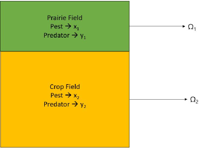
Figure 1. Visual depiction of the underlying assumptions regarding patches $\Omega_{1}\ \&\ \Omega_{2}$.

Our findings in the current manuscript are as follows,

• Unbounded growth of the predator population (without dispersal) can be mitigated with sufficient linear dispersal, in the patch model, via theorem 3.

• The patch model enables pest extinction in the crop field, via lemma 5.

• The patch model enables chaotic dynamics, see Fig. 10.

• The patch model has other rich dynamics such as the formation of limit cycles, via theorem 4.

• We discuss consequences of these results to AF driven bio-control that would utilize prairie strips, and so could be integrated with landscape management strategies and programs such as the STRIPs program in Iowa, and the mid western US.

4. Blow-up prevention

As seen in the earlier section, Blow-up phenomenon is seen in many AF models in the literature. That is they enable infinite time blow-up in the predator population, so must be applied to bio-control scenarios with caution. A basic AF model with a monotone pest dependent response, is unable to yield $(0,y^{*})$, the pest extinction state for $y^{*}<\infty$, and what is seen (see table ) that if $\xi>\xi_{critical}$, $(x,y)\rightarrow(0,\infty)$. Thus, blow-up prevention and the attainability of the (finite) $(0,y^{*})$ pest extinction state, is much sought after. To this end the introduced patch model is useful. We state the following theorem,

Theorem 3.

Consider the additional food patch model (3.1) with $\epsilon_{1}>\delta_{1},\epsilon_{2}>\delta_{2}$. If $k_{2}=k_{4}=0$, that is there is no dispersal between patches and $\xi>\xi_{critical}=\dfrac{\delta_{1}}{\epsilon_{1}-\alpha\delta_{1}}$, then the predator population blows up in infinite time. However with dispersal, that is $k_{2},k_{4}>0$ s.t., $\epsilon_{1}-\delta_{1}+k_{4}<k_{2}$, the predator population remains bounded for all time.

Proof.

Note the prey populations $x_{1},x_{2}$ are always bounded in comparison to the logistic equation. In the no dispersal case $k_{2}=k_{4}=0$, if $\xi>\xi_{critical}=\dfrac{\delta_{1}}{\epsilon_{1}-\alpha\delta_{1}}$, then blow-up in infinite time follows from [25]. Now, in the case of dispersal, we add up the predator equations to obtain,

$$\dot{y_{1}}+\dot{y_{2}}$$

$$= \epsilon_{1}\left(\frac{x_{1}+\xi}{1+x_{1}+\alpha\xi}\right)\ y_{1}-\delta_{1}y_{1}+k_{2}\left(y_{2}-y_{1}\right)$$

$$+ \epsilon_{2}\left(\frac{x_{2}}{1+x_{2}}\right)\ y_{2}-\delta_{2}y_{2}+k_{4}\left(y_{1}-y_{2}\right)$$

$$\leq \left(\epsilon_{1}y_{1}-\delta_{1}y_{1}+k_{2}\left(y_{2}-y_{1}\right)\right)+\left(\epsilon_{2}y_{2}-\delta_{2}y_{2}+k_{4}\left(y_{1}-y_{2}\right)\right)$$

$$= \left(\epsilon_{1}-\delta_{1}-k_{2}+k_{4}\right)y_{1}+\left(\epsilon_{2}-\delta_{2}-k_{4}+k_{2}\right)y_{2}$$

This follows via positivity of the solutions and under the assumption that $\xi<1+\alpha\xi$. Note if

(4.2) $$\epsilon_{1}-\delta_{1}-k_{2}+k_{4}\leq 0,$$

Then it follows that,

(4.3) $$\epsilon_{2}-\delta_{2}-k_{4}+k_{2}>0$$

Lets proceed by contradiction. Assume $y_{1},y_{2}$ blow-up in infinite time. Then $(y_{1})^{{}^{\prime}},(y_{2})^{{}^{\prime}}$ also blow up.

Now from the parametric assumptions we have,

(4.4) $$\dot{y_{1}}+\dot{y_{2}}<\left(-k_{2}+k_{4}\right)y_{1}+\left(\epsilon_{2}-\delta_{2}-k_{4}+k_{2}\right)y_{2}$$

Thus taking limits entails,

(4.5) $$\lim_{t\rightarrow\infty}\left(\dot{y_{1}}+\dot{y_{2}}+\left(k_{2}-k_{4}\right)y_{1}\right)=\infty<\lim_{t\rightarrow\infty}\left(\epsilon_{2}-\delta_{2}-k_{4}+k_{2}\right)y_{2}=\infty$$

this yields a contradiction. Also, note this follows as the rate of blow-up of $y_{2}$ cannot be any faster than the rate of blow-up of $y_{1}$, via inspection of the equation for $y_{2}$, and the earlier mentioned parametric restrictions. Thus both $y_{1},y_{2}$ don’t blow-up or one does and the other does not. If $y_{1}$ does blow-up but $y_{2}$ does not, we can integrate the equation for $y_{2}$, and use positivity to obtain,

(4.6) $$y_{2}(t)>k_{4}\int^{t}_{0}y_{1}(s)ds-(\delta_{2}+k_{4})\int^{t}_{0}y_{2}(s)ds-y_{2}(0)$$

Note, that the blow-up in $y_{1}$ must be exponential. Thus, taking limits we obtain,

$$\infty>C_{2}>\lim_{t\rightarrow\infty}(y_{2}(t))$$

$$> k_{4}\lim_{t\rightarrow\infty}\int^{t}_{0}y_{1}(s)ds-(\delta_{2}+k_{4})\int^{t}_{0}y_{2}(s)ds-y_{2}(0)$$

$$> k_{4}\lim_{t\rightarrow\infty}\int^{t}_{0}e^{C_{1}s}ds-(\delta_{2}+k_{4})\lim_{t\rightarrow\infty}\int^{t}_{0}C_{2}ds-y_{2}(0)$$

$$> \lim_{t\rightarrow\infty}\left(\frac{k_{4}}{C_{1}}\left(e^{C_{1}t}-1\right)-(\delta_{2}+k_{4})C_{2}t-C_{3}\right)$$

$$= \infty$$

Herein $C_{3}$ is an arbitrary constant that could depend on the initial data, and $C_{2}$ is the assumed bound on $y_{2}$, that could also depend on the initial data. Thus we obtain a contradiction. Similarly, we can derive a contradiction if $y_{2}$ does blow-up but $y_{1}$ does not. The result follows.

∎

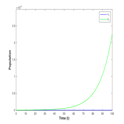
(a) $k_{2}=0,\ k_{4}=0$

(b) $k_{2}=0.45,\ k_{4}=0.2$

Figure (2(a)) shows the blow-up dynamics in predator population when $\xi>\xi_{critical}$ and no dispersal in (3.1) i.e., $k_{2}=k_{4}=0$. Figure (2(b)) shows the blow-up prevention in patch $\Omega_{1}$, when there is dispersal between the patches, i.e., $k_{2},k_{4}\neq 0$. In both simulations, the values of all other parameters remain constant, demonstrating that the movement of predators can prevent blow up in predator populations. Here, the parameter set used is $k=10,\alpha=0.2,\xi=0.8,\epsilon_{1}=\epsilon_{2}=0.4,\delta_{1}=\delta_{2}=0.2$ with I.C. $=[10,10,10,10]$. The values of $k_{2}\ \&\ k_{4}$ are selected based on the parametric constraints outlined in theorem 3.

Conjecture 1.

Consider the additional food patch model (3.1) with $\epsilon_{1}>\delta_{1},\epsilon_{2}>\delta_{2}$ and, $\xi>\xi_{critical}=\dfrac{\delta_{1}}{\epsilon_{1}-\alpha\delta_{1}}$. The predator population will remain bounded for all time if $k_{2},k_{4}>0$ s.t., $\epsilon_{2}-\delta_{2}+k_{2}<k_{4}$ and, $k_{2}>\epsilon_{1}-\delta_{1}$.

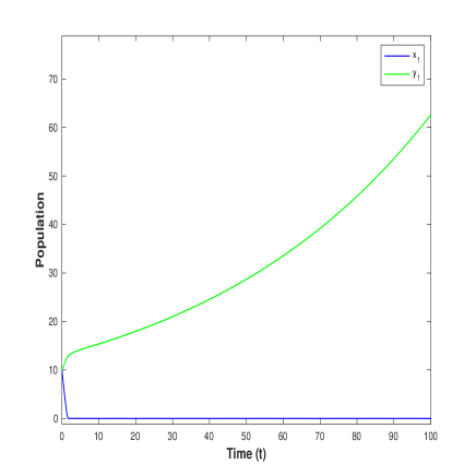
(a) $k_{2}=0.2,\ k_{4}=0.5$

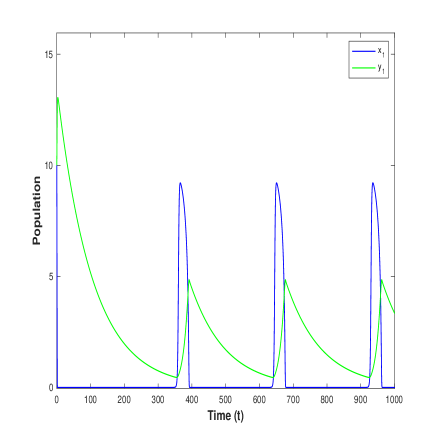
(b) $k_{2}=0.4,\ k_{4}=0.7$

Figure (3(a)) shows $k_{4}>k_{2}+\epsilon_{2}-\delta_{2}$ could not prevent a blow-up since, $k_{2}=\epsilon_{1}-\delta_{1}$, whereas figure (3(b)) shows that blow up can be prevented if $k_{2}>\epsilon_{1}-\delta_{1}$ then, $k_{4}>k_{2}+\epsilon_{2}-\delta_{2}$. Here, the parameter set used is $k=10,\alpha=0.2,\xi=0.8,\epsilon_{1}=\epsilon_{2}=0.4,\delta_{1}=\delta_{2}=0.2$ with I.C. $=[10,10,10,10]$. The values of $k_{2}\ \&\ k_{4}$ are selected based on the parametric constraints outlined in conjecture 1.

5. Equilibrium Analysis

We now consider the existence and local stability analysis of the biologically relevant equilibrium points for the system (3.1).

5.1. Existence of Equilibrium points

5.1.1. Pest free state in patch $\Omega_{2}:E_{1}=(x_{1}^{*},y_{1}^{*},0,y_{2}^{*})$

Lemma 1.

The equilibrium point $E_{1}=(x_{1}^{*},y_{1}^{*},0,y_{2}^{*})$ exists if $\xi<\dfrac{Q}{\epsilon_{1}-\alpha Q}$ and $\epsilon_{1}>Q$ where, $Q=\dfrac{\delta_{1}\delta_{2}+\delta_{1}k_{4}+k_{2}\delta_{2}}{\delta_{2}+k_{4}}$.

See Appendix (10.1)

5.1.2. Pest free state in patch $\Omega_{1}:E_{2}=(0,y_{1}^{*},x_{2}^{*},y_{2}^{*})$

Lemma 2.

The equilibrium point $E_{2}=(0,y_{1}^{*},x_{2}^{*},y_{2}^{*})$ exists if, $\tilde{Q}>0$ and $\epsilon_{2}>\tilde{Q}$ where, $\tilde{Q}=\delta_{2}+k_{4}+\dfrac{k_{2}\ k_{4}}{\dfrac{\epsilon_{1}\xi}{1+\alpha\xi}\ -\delta_{1}-k_{2}}$.

See Appendix (10.2)

5.1.3. Pest free state in both $\Omega_{1}\ \&\ \Omega_{2}:E_{3}=(0,y_{1}^{*},0,y_{2}^{*})$

Lemma 3.

The equilibrium point $E_{3}=(0,y_{1}^{*},0,y_{2}^{*})$ exists if $\xi=\dfrac{{Q}}{\epsilon_{1}-\alpha{Q}}$ where, $Q=\dfrac{\delta_{1}\delta_{2}+\delta_{1}k_{4}+k_{2}\delta_{2}}{\delta_{2}+k_{4}}$.

See Appendix (10.3)

5.1.4. Coexistence equilibrium point

Lemma 4.

The equilibrium point $E_{4}=(x_{1}^{\star},y_{1}^{\star},x_{2}^{\star},y_{2}^{\star})$ exists if $0<x_{1}^{\star}<\dfrac{\delta_{1}+k_{2}}{\epsilon_{1}-(\delta_{1}+k_{2})}-\alpha\xi$, $0<x_{2}^{\star}<\dfrac{\delta_{2}+k_{4}}{\epsilon_{2}-(\delta_{2}+k_{4})}$, where $x_{2}^{\star}=f(x_{1}^{\star})$ and $x_{1}^{\star}$ can be solved from nullcline equations.

See Appendix (10.4)

5.2. Local Stability Analysis of Equilibrium points

The Jacobian matrix $(J)$ for the additional food patch model (3.1) is given by:

(5.1) $$J=\begin{bmatrix}1-\dfrac{2x_{1}}{k}-\dfrac{y_{1}\left(1+\alpha\xi\right)}{\left(1+x_{1}+\alpha\xi\right)^{2}}&\dfrac{-x_{1}}{1+x_{1}+\alpha\xi}&0&0\vspace{0.25cm}\\ \dfrac{\epsilon_{1}\left(1+\left(\alpha-1\right)\xi\right)\ y_{1}}{(1+x_{1}+\alpha\xi)^{2}}&\epsilon_{1}\dfrac{\left(x_{1}+\xi\right)}{1+x_{1}+\alpha\xi}-\delta_{1}-k_{2}&0&k_{2}\\ 0&0&1-\dfrac{2x_{2}}{k}-\dfrac{y_{2}}{(1+x_{2})^{2}}&\dfrac{-x_{2}}{1+x_{2}}\vspace{0.25cm}\\ 0&k_{4}&\dfrac{\epsilon_{2}y_{2}}{(1+x_{2})^{2}}&\dfrac{\epsilon_{2}x_{2}}{1+x_{2}}-\delta_{2}-k_{4}\end{bmatrix}$$

By evaluating this Jacobian matrix at each equilibrium point, we obtain the local stability conditions of $E_{1},E_{2},E_{3}$ and $E_{4}$.

5.2.1. Stability Analysis for pest free state in patch $\Omega_{2}$

Lemma 5.

The equilibrium point $E_{1}=(x_{1}^{*},y_{1}^{*},0,y_{2}^{*})$ is conditionally locally asymptotically stable.

Proof.

Using equations (10.1) and (10.2), the general Jacobian matrix (5.1) at $(x_{1}^{*},y_{1}^{*},0,y_{2}^{*})$ becomes

$$J_{1}=\begin{bmatrix}\dfrac{x_{1}^{*}y_{1}^{*}}{(1+x_{1}^{*}+\alpha\xi)^{2}}-\dfrac{x_{1}^{*}}{k}&\dfrac{-x_{1}^{*}}{1+x_{1}^{*}+\alpha\xi}&0&0\vspace{0.25cm}\\ \dfrac{\epsilon_{1}(1+(\alpha-1)\xi)\ y_{1}^{*}}{(1+x_{1}^{*}+\alpha\xi)^{2}}&-\dfrac{k_{2}k_{4}}{\delta_{2}+k_{4}}&0&k_{2}\vspace{0.25cm}\\ 0&0&1-y_{2}^{*}&0\vspace{0.25cm}\\ 0&k_{4}&\epsilon_{2}y_{2}^{*}&-\delta_{2}-k_{4}\end{bmatrix}$$

The characteristic polynomial comes out as:

$$=\left(1-y_{2}^{*}-\lambda\right)\left[\left(\dfrac{x_{1}^{*}y_{1}^{*}}{(1+x_{1}^{*}+\alpha\xi)^{2}}-\dfrac{x_{1}^{*}}{k}-\lambda\right)\left(\lambda^{2}+\lambda\left(\dfrac{k_{2}y_{2}^{*}}{y_{1}^{*}}+\dfrac{k_{4}y_{1}^{*}}{y_{2}^{*}}\right)\right)\right]$$

$$+\left(1-y_{2}^{*}-\lambda\right)\left[\left(\dfrac{x_{1}^{*}}{1+x_{1}^{*}+\alpha\xi}\right)\left(\dfrac{-k_{4}y_{1}^{*}}{y_{2}^{*}}-\lambda\right)\left(\dfrac{\epsilon_{1}(1+(\alpha-1)\xi)\ y_{1}^{*}}{(1+x_{1}^{*}+\alpha\xi)^{2}}\right)\right]$$

$$\text{Let, }D=1-y_{2}^{*},\ A=\dfrac{x_{1}^{*}y_{1}^{*}}{(1+x_{1}^{*}+\alpha\xi)^{2}}-\dfrac{x_{1}^{*}}{k},\ B=\dfrac{x_{1}^{*}}{1+x_{1}^{*}+\alpha\xi},\ C=\dfrac{\epsilon_{1}(1+(\alpha-1)\xi)\ y_{1}^{*}}{(1+x_{1}^{*}+\alpha\xi)^{2}},$$

$$\ P=\dfrac{k_{2}y_{2}^{*}}{y_{1}^{*}}+\dfrac{k_{4}y_{1}^{*}}{y_{2}^{*}},\ E=\dfrac{k_{4}y_{1}^{*}}{y_{2}^{*}}\text{ where }B,P,E>0$$

Now the characteristic equation becomes,

$$\implies\left(D-\lambda\right)\{\left(A-\lambda\right)\left(\lambda^{2}+P\lambda\right)+BC\left(-E-\lambda\right)\}=0$$

$$\implies\lambda^{4}-\lambda^{3}\left(A-P+D\right)+\lambda^{2}\left(D(A-P)-(AP-BC)\right)+\lambda\left(D(AP-BC)+BCE\right)-BCDE=0$$

$$\implies\lambda^{4}+A_{3}\lambda^{3}+A_{2}\lambda^{2}+A_{1}\lambda+A_{0}=0$$

$$\text{where, }A_{3}=-\left(A-P+D\right),\ A_{2}=D(A-P)-(AP-BC),\ A_{1}=D(AP-BC)+BCE,\ A_{0}=-BCDE$$

From the Routh–Hurwitz stability criteria, we should have the following conditions:

$$A_{3}>0,A_{2}>0,A_{1}>0,A_{0}>0,\text{ and }A_{3}A_{2}A_{1}>A_{1}^{2}+A_{3}^{2}A_{0}.$$

(5.2) $$\text{for}A_{0}>0,-BCDE>0\implies BCDE<0\text{ as }B,E>0,C>0\text{ (due to feasibility condition)}\implies D<0$$

$$\text{for }A_{1}>0,D(AP-BC)+BCE>0$$

$$\text{for }A_{2}>0,D(A-P)-(AP-BC)>0\implies D(A-P)>AP-BC$$

$$\text{for }A_{3}>0,-\left(A-P+D\right)>0\implies\left(A-P+D\right)<0$$

$$\text{for }A_{3}A_{2}A_{1}>A_{1}^{2}+A_{3}^{2}A_{0}\text{ we have,}$$

$$\implies-\left(A-P+D\right)\left(D(A-P)-(AP-BC)\right)\left(D(AP-BC)+BCE\right)$$

$$\hskip 28.45274pt>\left(D(AP-BC)+BCE\right)^{2}-\left(A-P+D\right)^{2}BCDE$$

$$\implies(A-P)(AP-BC)(D^{3}+D^{2}(A-P)-D(AP-BC)-BCE)$$

$$\hskip 28.45274pt<BCE(D^{3}+D^{2}(A-P)-D(AP-BC)-BCE)$$

$$\because\ (D^{3}+D^{2}(A-P)-D(AP-BC)-BCE)<0\implies(A-P)(AP-BC)>BCE$$

∎

Figure 4. The time series figure shows pest extinction in patch $\Omega_{2}$. The parameters used are $k=10,\alpha=0.2,\xi=0.39,\epsilon_{1}=\epsilon_{2}=0.4,\delta_{1}=\delta_{2}=0.2,k_{2}=0.3,k_{4}=0.2$ with I.C. $=[5,3,0.2,1.5]$.

Figure 5. The time series figure shows pest extinction in patch $\Omega_{2}$. Initially, the predators are introduced solely in $\Omega_{1}$, and due to their dispersion, predators enter the crop field and subsequently eliminate pest. The parameters used are $k=10,\alpha=0.2,\xi=0.39,\epsilon_{1}=\epsilon_{2}=0.4,\delta_{1}=\delta_{2}=0.2,k_{2}=0.3,k_{4}=0.2$ with I.C. $=[5,3,0.05,0]$.

5.2.2. Stability Analysis for pest free state in patch $\Omega_{1}$

Lemma 6.

The equilibrium point $E_{2}=(0,y_{1}^{*},x_{2}^{*},y_{2}^{*})$ is conditionally locally asymptotically stable.

Proof.

Using equations (10.5), (10.6) and (10.7), the general Jacobian matrix (5.1) at $(0,y_{1}^{*},x_{2}^{*},y_{2}^{*})$ becomes,

$$J_{2}=\begin{bmatrix}1-\dfrac{y_{1}^{*}}{\left(1+\alpha\xi\right)}&0&0&0\vspace{0.25cm}\\ \dfrac{\epsilon_{1}\left(1+\left(\alpha-1\right)\xi\right)\ y_{1}^{*}}{(1+\alpha\xi)^{2}}&\dfrac{-k_{2}y_{2}^{*}}{y_{1}^{*}}&0&k_{2}\vspace{0.25cm}\\ 0&0&\dfrac{x_{2}^{*}y_{2}^{*}}{\left(1+x_{2}^{*}\right)^{2}}-\dfrac{x_{2}^{*}}{k}&\dfrac{-x_{2}^{*}}{1+x_{2}^{*}}\vspace{0.25cm}\\ 0&k_{4}&\dfrac{\epsilon_{2}y_{2}^{*}}{(1+x_{2}^{*})^{2}}&\dfrac{-k_{4}y_{1}^{*}}{y_{2}^{*}}\end{bmatrix}$$

The characteristic equation is given by:

$$\left(1-\dfrac{y_{1}^{*}}{1+\alpha\xi}-\lambda\right)\left[\left(\dfrac{x_{2}^{*}y_{2}^{*}}{\left(1+x_{2}^{*}\right)^{2}}-\dfrac{x_{2}^{*}}{k}-\lambda\right)\left(\lambda^{2}+\lambda\left(\dfrac{k_{2}y_{2}^{*}}{y_{1}^{*}}+\dfrac{k_{4}y_{1}^{*}}{y_{2}^{*}}\right)\right)+\left(\dfrac{-k_{2}y_{2}^{*}}{y_{1}^{*}}-\lambda\right)\left(\dfrac{\epsilon_{2}x_{2}^{*}y_{2}^{*}}{(1+x_{2}^{*})^{3}}\right)\right]=0$$

$$\text{Let, }D=\left(1-\dfrac{y_{1}^{*}}{1+\alpha\xi}\right),\hskip 7.11317ptA=\dfrac{x_{2}^{*}y_{2}^{*}}{\left(1+x_{2}^{*}\right)^{2}}-\dfrac{x_{2}^{*}}{k},\hskip 7.11317ptC=\dfrac{\epsilon_{2}x_{2}^{*}y_{2}^{*}}{(1+x_{2}^{*})^{3}},\hskip 7.11317ptP=\dfrac{k_{2}y_{2}^{*}}{y_{1}^{*}}+\dfrac{k_{4}y_{1}^{*}}{y_{2}^{*}},\hskip 7.11317ptE=\dfrac{k_{2}y_{2}^{*}}{y_{1}^{*}}$$

where $C,P,E>0$

Now the characteristic equation becomes, $(D-\lambda)\left[\left(A-\lambda\right)\left(\lambda^{2}+P\lambda\right)+\left(-E-\lambda\right)C\right]=0$

$$\implies \lambda^{4}-\lambda^{3}\left(A-P+D\right)+\lambda^{2}\left(D(A-P)-(AP-C)\right)+\lambda\left(D(AP-C)+CE\right)-CDE=0$$

$$\implies \lambda^{4}+A_{3}\lambda^{3}+A_{2}\lambda^{2}+A_{1}\lambda+A_{0}=0$$

where,
$A_{3}=-\left(A-P+D\right)$, $A_{2}=\left(D(A-P)-(AP-C)\right)$, $A_{1}=\left(D(AP-C)+CE\right)$, $A_{0}=-CDE$

From the Routh–Hurwitz stability criteria, we should have the following conditions: $A_{3}>0$, $A_{2}>0$, $A_{1}>0$, $A_{0}>0$, and $A_{3}A_{2}A_{1}>A_{1}^{2}+A_{3}^{2}A_{0}$.

(5.3) $$\text{ for }A_{0}>0,-CDE>0\implies CDE<0\text{ as }E,C>0\implies D<0$$

$$\text{ for }A_{1}>0,D(AP-C)+CE>0$$

$$\text{ for }A_{2}>0,D(A-P)-(AP-C)>0\implies D(A-P)>AP-C$$

$$\text{ for }A_{3}>0,-\left(A-P+D\right)>0\implies\left(A-P+D\right)<0$$

$$\text{ for }A_{3}A_{2}A_{1}>A_{1}^{2}+A_{3}^{2}A_{0}\text{ we have},$$

$$-\left(A-P+D\right)\left(D(A-P)-(AP-C)\right)\left(D(AP-C)+CE\right)>\left(D(AP-C)+CE\right)^{2}-\left(A-P+D\right)^{2}CDE$$

$$\implies(A-P)(AP-C)(D^{3}+D^{2}(A-P)-D(AP-C)-CE)<CE(D^{3}+D^{2}(A-P)-D(AP-C)-CE)$$

$$\because(D^{3}+D^{2}(A-P)-D(AP-C)-CE)<0\implies(A-P)(AP-C)>CE$$

∎

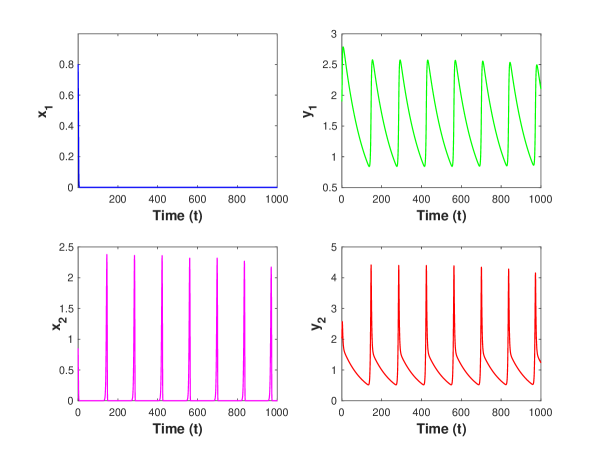
Figure 6. The time series figure shows pest extinction in patch $\Omega_{1}$. The parameters used are $k=10,\alpha=0.2,\xi=0.5,\epsilon_{1}=0.4,\epsilon_{2}=0.8,\delta_{1}=\delta_{2}=0.15,k_{2}=0.1,k_{4}=0.2$ with I.C. $=[0.8,1.9,0.85,2.03]$.

5.2.3. Stability Analysis for pest free state in both $\Omega_{1}\ \&\ \Omega_{2}$

Lemma 7.

The equilibrium point $E_{3}=(0,y_{1}^{*},0,y_{2}^{*})$ is a non-hyperbolic point.

Proof.

Using equation (10.10), the general Jacobian matrix (5.1) at $(0,y_{1}^{*},0,y_{2}^{*})$ we have,

$$J_{3}=\begin{bmatrix}1-\dfrac{y_{1}^{*}}{(1+\alpha\xi)}&0&0&0\vspace{0.25cm}\\ \dfrac{\epsilon_{1}(1+(\alpha-1)\xi)\ y_{1}^{*}}{(1+\alpha\xi)^{2}}&\dfrac{-k_{2}k_{4}}{\delta_{2}+k_{4}}&0&k_{2}\vspace{0.25cm}\\ 0&0&1-y_{2}^{*}&0\vspace{0.25cm}\\ 0&k_{4}&\epsilon_{2}y_{2}^{*}&-\delta_{2}-k_{4}\end{bmatrix}$$

The characteristic equation is given by:

$$\lambda\left(1-\dfrac{y_{1}^{*}}{1+\alpha\xi}-\lambda\right)\left(1-y_{2}^{*}-\lambda\right)\left(\lambda+\left(\dfrac{k_{2}k_{4}}{\delta_{2}+k_{4}}+\delta_{2}+k_{4}\right)\right)=0$$

$$\lambda_{1}=0,\hskip 5.69046pt\lambda_{2}=1-y_{2}^{*},\hskip 5.69046pt\lambda_{3}=1-\dfrac{y_{1}^{*}}{1+\alpha\xi}\hskip 5.69046pt,\lambda_{4}=-\left(\dfrac{k_{2}k_{4}}{\delta_{2}+k_{4}}+\delta_{2}+k_{4}\right)$$

∎

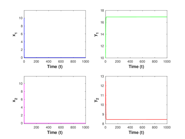
Figure 7. The time series figure shows pest extinction in both patches $\Omega_{1}$ & $\Omega_{2}$ for an exact quantity of additional food. The parameters used are $k=20,\alpha=0.2,\xi=1.06061,\epsilon_{1}=\epsilon_{2}=0.4,\delta_{1}=\delta_{2}=0.2,k_{2}=0.3,k_{4}=0.2$ with I.C. $=[10,10,10,10]$.

5.2.4. Stability analysis for coexistence equilibrium

Lemma 8.

The equilibrium point $E_{4}=(x_{1}^{\star},y_{1}^{\star},x_{2}^{\star},y_{2}^{\star})$ is conditionally locally asymptotically stable.

Proof.

The general Jacobian matrix (5.1) at $(x_{1}^{\star},y_{1}^{\star},x_{2}^{\star},y_{2}^{\star})$ becomes,

$$J_{4}=\begin{bmatrix}J_{11}&J_{12}&0&0\\ J_{21}&J_{22}&0&J_{24}\\ 0&0&J_{33}&J_{34}\\ 0&J_{42}&J_{43}&J_{44}\end{bmatrix}$$

$$\text{where, }J_{11}=1-\dfrac{2x_{1}^{\star}}{k}+\dfrac{\left(1-\dfrac{x_{2}^{\star}}{k}\right)\left(1+\alpha\xi\right)\left\{\epsilon_{2}x_{2}^{\star}-(\delta_{2}+k_{4})(1+x_{2}^{\star})\right\}}{k_{4}\left(1+x_{1}^{\star}+\alpha\xi\right)^{2}},\ J_{12}=\dfrac{-x_{1}^{\star}}{1+x_{1}^{\star}+\alpha\xi}$$

$$J_{21}=\dfrac{-\epsilon_{1}\left(1-\dfrac{x_{2}^{\star}}{k}\right)\left(1+\left(\alpha-1\right)\xi\right)\ \left\{\epsilon_{2}x_{2}^{\star}-(\delta_{2}+k_{4})(1+x_{2}^{\star})\right\}}{k_{4}(1+x_{1}^{\star}+\alpha\xi)^{2}},\ J_{22}=\epsilon_{1}\dfrac{\left(x_{1}^{\star}+\xi\right)}{1+x_{1}^{\star}+\alpha\xi}-\delta_{1}-k_{2}$$

$$J_{24}=k_{2},\ J_{33}=1-\dfrac{2x_{2}^{\star}}{k}+\dfrac{\left(1-\dfrac{x_{1}^{\star}}{k}\right)\left\{\epsilon_{1}(x_{1}^{\star}+\xi)-(\delta_{1}+k_{2})(1+x_{1}^{\star}+\alpha\xi)\right\}}{k_{2}(1+x_{2}^{\star})^{2}},\ J_{34}=\dfrac{-x_{2}^{\star}}{1+x_{2}^{\star}},$$

$$J_{42}=k_{4},\ J_{43}=\dfrac{-\epsilon_{2}\left(1-\dfrac{x_{1}^{\star}}{k}\right)\left\{\epsilon_{1}(x_{1}^{\star}+\xi)-(\delta_{1}+k_{2})(1+x_{1}^{\star}+\alpha\xi)\right\}}{k_{2}(1+x_{2}^{\star})^{2}},\ J_{44}=\dfrac{\epsilon_{2}x_{2}^{\star}}{1+x_{2}^{\star}}-\delta_{2}-k_{4}$$

The characteristic equation is given by, $\lambda^{4}+A\lambda^{3}+B\lambda^{2}+C\lambda+D=0$ where,

$$A=-(J_{11}+J_{22}+J_{33}+J_{44}),\hskip 1.42271ptB=J_{11}J_{22}+J_{33}J_{44}+J_{12}J_{21}-(J_{34}J_{43}+J_{24}J_{42})+(J_{11}+J_{22})(J_{33}+J_{44})$$

$$C=(J_{11}+J_{33})J_{24}J_{42}-(J_{33}+J_{44})(J_{11}J_{22}+J_{12}J_{21})-(J_{11}+J_{22})(J_{33}J_{44}-J_{34}J_{43})$$

$$D=(J_{11}J_{22}+J_{12}J_{21})(J_{33}J_{44}-J_{34}J_{43})-J_{11}J_{24}J_{33}J_{42}$$

From the Routh–Hurwitz stability criteria, we should have the following conditions:

(5.4) $$A>0,B>0,C>0,D>0,\And ABC>C^{2}+A^{2}D$$

∎

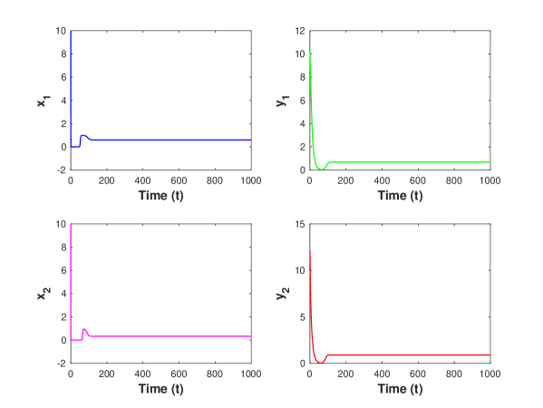
Figure 8. The time series figure shows the coexistence state in both patches $\Omega_{1}$ & $\Omega_{2}$. The parameters used are $k=1,\alpha=0.2,\xi=0.37,\epsilon_{1}=0.2,\epsilon_{2}=0.8,\delta_{1}=\delta_{2}=0.15,k_{2}=0.1,k_{4}=0.2$ with I.C.$=[10,10,10,10]$.

6. Hopf Bifurcation

The bifurcation point is the critical parameter value at which the qualitative dynamics of a model change. The bifurcation parameter in our mathematical model (3.1) is $\xi$, the quantity of additional food. For Hopf Bifurcation, we are using the method developed in [18]. the following conditions need to hold for the bifurcation parameter $\xi=\xi^{*}$

Theorem 4.

The necessary and sufficient conditions for the system (3.1) undergoes Hopf bifurcation with respect to the parameter $\xi=\xi^{*}$ around the equilibrium point $E_{1}=(x_{1}^{*},y_{1}^{*},0,y_{2}^{*})$ are stated as follows:

1. $A_{0}(\xi^{*})>0$, $A_{3}(\xi^{*})>0$, $(A_{3}A_{2}-A_{1})(\xi^{*})>0$
   

2. $f(\xi^{*})=(A_{1}A_{2}A_{3}-A_{0}A_{3}^{2}-A_{1}^{2})(\xi^{*})=0$
   

3. $\derivative{(f(\xi))}{\xi}\rvert_{\xi=\xi^{*}}\neq 0$

Proof.

The characteristic equation for $J_{1}=J(E_{1})$ is given by:

$$\hskip 170.71652pt\lambda^{4}+A_{3}\lambda^{3}+A_{2}\lambda^{2}+A_{1}\lambda+A_{0}=0$$

$$\text{where, }A_{3}=-\left(A-P+D\right),\ A_{2}=D(A-P)-(AP-BC),\ A_{1}=D(AP-BC)+BCE,\ A_{0}=-BCDE$$

$$\text{ for }A_{0}(\xi^{*})>0\implies BCDE(\xi^{*})<0\text{ ( which is always true from the feasibility condition )}$$

$$\text{ for }A_{3}(\xi^{*})>0\implies(A-P+D)(\xi^{*})<0$$

$$\text{ for }(A_{3}A_{2}-A_{1})(\xi^{*})>0\implies(A-P+D)\left(D(A-P)-(AP-BC)\right)+\left(D(AP-BC)+BCE\right)<0\rvert_{\xi=\xi^{*}}$$

$$\text{ for }f(\xi^{*})=(A_{1}A_{2}A_{3}-A_{0}A_{3}^{2}-A_{1}^{2})(\xi^{*})=0\text{ we have,}$$

$$\implies-(A-P+D)\left(D(A-P)-(AP-BC)\right)\left(D(AP-BC)+BCE\right)$$

$$\hskip 28.45274pt+BCDE(A-P+D)^{2}-\left(D(AP-BC)+BCE\right)^{2}\rvert_{\xi=\xi^{*}}=0$$

$$\implies\{D^{3}+D^{2}(A-P)-D(AP-BC)-BCE\}*\{(A-P)(AP-BC)-BCE\}\rvert_{\xi=\xi^{*}}=0$$

$$\text{ for }\derivative{(f(\xi))}{\xi}\rvert_{\xi=\xi^{*}}\neq 0\implies\derivative{(A_{1}A_{2}A_{3}-A_{0}A_{3}^{2}-A_{1}^{2})}{\xi}\rvert_{\xi=\xi^{*}}\neq 0$$

$$\text{Now, using the above expression we solve, }\derivative{(\phi*\psi)}{\xi}\rvert_{\xi=\xi^{*}}=\phi*\derivative{\psi}{\xi}+\psi*\derivative{\phi}{\xi}\rvert_{\xi=\xi^{*}}\neq 0$$

$$\text{where, }\phi(\xi)=D^{3}+D^{2}(A-P)-D(AP-BC)-BCE,\hskip 8.5359pt\psi(\xi)=(A-P)(AP-BC)-BCE$$

∎

7. Chaos

A commonly seen dynamic in multi-component ODE systems, that is typically systems of three or more ODE, is chaos. This is defined as aperiodic behavior exhibiting sensitive dependence to initial condition [7]. We explored the possibility of chaotic dynamics of our proposed system (3.1). We used the parameter set $K=70,\alpha=0.2,\epsilon_{1}=\epsilon_{2}=0.4,\delta_{1}=0.2,\delta_{2}=0.16,k_{1}=k_{3}=0,k_{2}=0.3,k_{4}=0.2.$ The change in system dynamics is studied with a change in parameter $\xi$. The first evidence of chaos can be found when the solution of the system is very sensitive to initial value. In figure (14), we have considered two initial conditions differing by a factor of $10^{-14}$, and we see the divergence in both solutions in time series by taking the log difference of both solutions.

Using the above parameter set and taking $\xi=0.7$, we see that $x_{2}$ goes extinct while all other populations show limit cycle oscillations as seen in figure (9). When $\xi$ is decreased to $\xi=0.41212$, we see chaotic dynamics in $x_{2},y_{2},y_{1}$ populations as seen in time series in figure (10).

We look further into the validation of the chaotic dynamics by looking at the population variation with changing $\xi$ by studying the Lyapunov exponent. In figure (11), we see that for higher values of $\xi$, i.e. ($\xi>0.54$), we have stable max and min values of population $x_{2}$ but for lower values of $\xi$ we have all different values of $x_{2}$.

The chaotic dynamics are further investigated by studying the maximum Lyapunov exponent with respect to the parameter $\xi$ as seen in figure (13), and it can be analyzed that we get the maximum Lyapunov exponent as positive for different range of $\xi$ values. Thus, for the described parameter set, we can have chaos in windows of $\xi$ parameter values, one of which is $\xi=0.41212$. If we study the Lyapunov exponent for $\xi=0.41212$, we see that this is positive over time, which shows the divergence of solution, and which results in the chaotic dynamics as seen in figure (12).

Thus, we conclude the existence of chaotic dynamics in the system (3.1).

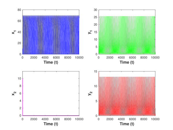
Figure 9. In the time series, we see the pest population in $\Omega_{2}$, go extinct while all other populations exhibit stable limit cycles for $k=70,\alpha=0.2,\xi=0.7,\epsilon_{1}\!=\epsilon_{2}=0.4,\delta_{1}=0.2,\delta_{2}=0.16,k_{2}=0.3,k_{4}=0.2$ with I.C. $=[10,10,10,10]$.

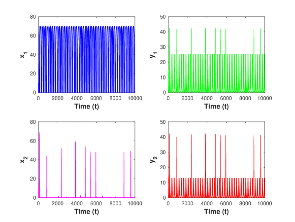
Figure 10. Chaotic dynamics can be seen in the $x_{2}$ population. The parameters used are $k=70,\alpha=0.2,\xi=0.41212,\epsilon_{1}=\epsilon_{2}=0.4,\delta_{1}=0.2,\delta_{2}=0.16,k_{2}=0.3,k_{4}=0.2$ with I.C. $=[10,10,10,10]$.

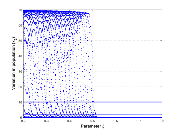
Figure 11. $k=70,\alpha=0.2,\xi=0.41212,\epsilon_{1}=\epsilon_{2}=0.4,\delta_{1}=0.2,\delta_{2}=0.16,k_{1}=k_{3}=0,k_{2}=0.3,k_{4}=0.2$ with I.C. $=[10,10,10,10]$.

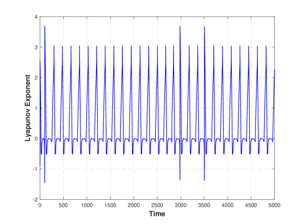
Figure 12. The positive Lyapunov shows divergence with respect to time, which shows chaos. The parameters used are $k=70,\alpha=0.2,\xi=0.41212,\epsilon_{1}=\epsilon_{2}=0.4,\delta_{1}=0.2,\delta_{2}=0.16,k_{2}=0.3,k_{4}=0.2$ with I.C. $=[10,10,10,10]$.

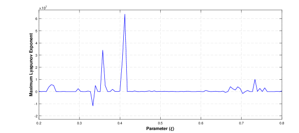
Figure 13. The graph shows the maximum Lyapunov exponent with respect to the parameter $\xi$. The graph shows chaotic dynamics at some $\xi$ values where the maximum Lyapunov is positive. The parameters used are $k=70,\alpha=0.2,\xi=0.41212,\epsilon_{1}=\epsilon_{2}=0.4,\delta_{1}=0.2,\delta_{2}=0.16,k_{2}=0.3,k_{4}=0.2$ with I.C. $=[10,10,10,10]$.

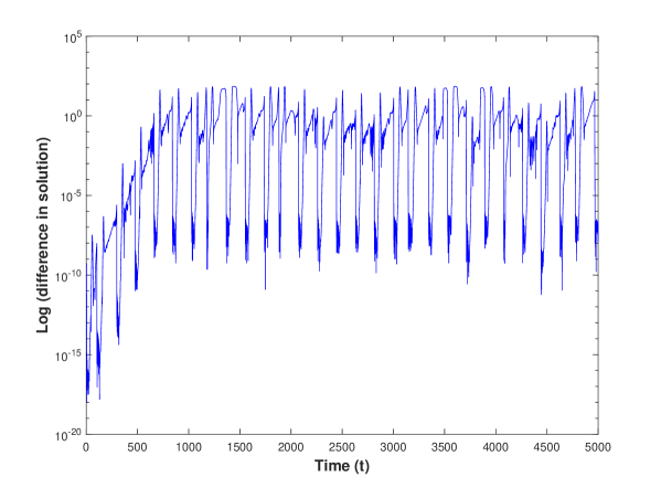
Figure 14. The graph shows the maximum Lyapunov exponent with respect to the parameter $\xi$. The graph shows chaotic dynamics at some $\xi$ values where the maximum Lyapunov is positive. The parameters used are $k=70,\alpha=0.2,\xi=0.41212,\epsilon_{1}=\epsilon_{2}=0.4,\delta_{1}=0.2,\delta_{2}=0.16,k_{2}=0.3,k_{4}=0.2$ with I.C. $=[10,10,10,10]$.

8. Comparison of AF patch model to classical bio-control models

In this section, we compare the classical models with our additional food two-patch model to show the benefits of this model in pest control. So, we study the possibilities of coexistence state in the models. We have studied the $(x^{*},{y}^{*})$ state in the Rosenzweig-MacArthur model and Holling type II additional food model and have studied the $(0,{y_{1}^{*}},{x_{2}^{*}},{y_{2}^{*}})$ state to compare the total pest population between all these models.

We also numerically investigate the comparison of pest levels concerning the interior state for all the above-mentioned models, i.e., comparing the $(x_{1}^{\star},y_{1}^{\star},x_{2}^{\star},y_{2}^{\star})$ of (3.1) with $(x^{*},{y}^{*})$ of (8.1) and (8.2).

8.1. Rosenzweig-MacArthur Predator-Prey model vs. Patch driven Additional food model

We first study the classical Rosenzweig-MacArthur model [37] which, if non-dimensionalized is given by:

(8.1) $$\dot{x_{r}} =x_{r}\bigg{(}1-\dfrac{x_{r}}{k}\bigg{)}-\dfrac{x_{r}y_{r}}{1+x_{r}}$$

$$\dot{y_{r}} =\dfrac{\epsilon_{2}x_{r}y_{r}}{1+x_{r}}-\delta_{2}y_{r}$$

The dynamics of the Rosenzweig-MacArthur (RM) model show that we cannot have pest extinction. So, the least pest population we can have is when interior equilibrium $(x_{r}^{*},y_{r}^{*})$ where $x_{r}^{*}=\dfrac{\delta_{2}}{\epsilon_{2}-\delta_{2}}$ and the interior is stable when $k<\dfrac{\delta_{2}+\epsilon_{2}}{\epsilon_{2}-\delta_{2}}$.

Lemma 9.

When $\dfrac{\delta_{1}}{\epsilon_{1}-\delta_{1}\alpha}<\xi<\dfrac{\delta_{1}+k_{2}}{\epsilon_{1}-\alpha(\delta_{1}+k_{2})}$ then system (3.1) can achieve lower pest population than system (8.1).

Proof.

We will compare the $(x_{r}^{*},y_{r}^{*})$ equilibrium of system (8.1) and the $(0,y_{1}^{*},x_{2}^{*},y_{2}^{*})$ equilibrium of system (3.1) where total pest population in the system is $x_{2}$. We know, $x^{*}_{r}=\dfrac{\delta_{2}}{\epsilon_{2}-\delta_{2}}$ and $x_{2}^{*}=\dfrac{\tilde{Q}}{\epsilon_{2}-\tilde{Q}}$, where, $\tilde{Q}=\delta_{2}+k_{4}+\dfrac{k_{2}\ k_{4}}{\dfrac{\epsilon_{1}\xi}{1+\alpha\xi}\ -\delta_{1}-k_{2}}.$ So, if $\dfrac{\epsilon_{1}\xi}{1+\alpha\xi}\ -\delta_{1}-k_{2}>0$ then $x_{2}^{*}>x_{r}^{*}$. Thus, in order for pest population to be lower in the system (3.1), we need $\tilde{Q}<\delta_{2}$. Solving, we get $\xi<\dfrac{\delta_{1}+k_{2}}{\epsilon_{1}-\alpha(\delta_{1}+k_{2})}$.

Now, if we solve $x_{2}^{*}<x_{r}^{*}$ we get, $\delta_{2}>\tilde{Q}$ i.e., $k_{2}<\delta_{1}+k_{2}-\dfrac{\epsilon_{1}\xi}{1+\alpha\xi}$.

Thus, we have a lower total pest population in the system (3.1) than in the system (8.1) when,

$$\dfrac{\delta_{1}}{\epsilon_{1}-\delta_{1}\alpha}<\xi<\dfrac{\delta_{1}+k_{2}}{\epsilon_{1}-\alpha(\delta_{1}+k_{2})}.$$

∎

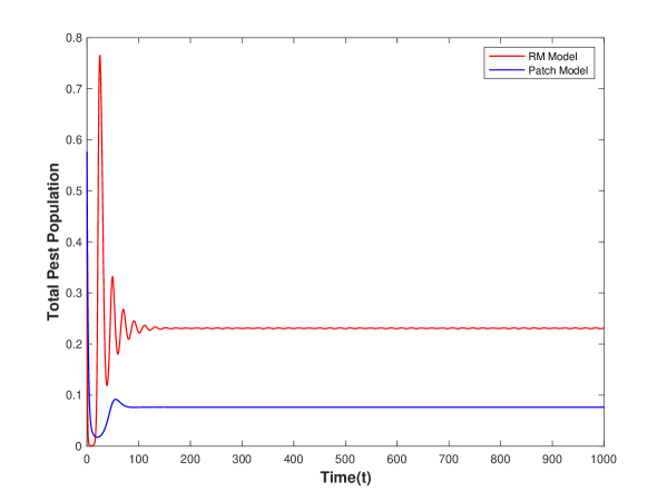
Figure 15. The time series figure showing the total pest population comparison of the system (8.1) and (3.1). The initial condition of the population for the patch model is [0.5, 1.56644, 0.0762332, 1.06803], and that for the RM model is used as total pest and predator population respectively, i.e. [0.5762, 2.6345].

Lemma 10.

When $\epsilon_{1}>Q\alpha$ and $0<\xi<\dfrac{Q(\epsilon_{1}-\delta_{1})-\delta_{1}(\epsilon_{1}-Q)}{(\epsilon_{1}-Q\alpha)(\epsilon_{1}-\delta_{1})}$ then system (3.1) can achieve higher pest population than system (8.1) where $Q=\dfrac{\delta_{1}\delta_{2}+\delta_{1}k_{4}+k_{2}\delta_{2}}{\delta_{2}+k_{4}}$.

Proof.

We prove the result using comparison. We will compare the $(x_{r}^{*},y_{r}^{*})$ equilibrium of system (8.1) and the $(x_{1}^{*},y_{1}^{*},0,y_{2}^{*})$ equilibrium of system (3.1) where total pest population in the system is $x_{1}$.

The equilibrium points can be stated as $x_{r}^{*}=\dfrac{\delta_{1}}{\epsilon_{1}-\delta_{1}}$ and $x_{1}^{*}=\dfrac{Q(1+\alpha\xi)-\epsilon_{1}\xi}{\epsilon_{1}-Q}$ where, $Q=\dfrac{\delta_{1}\delta_{2}+\delta_{1}k_{4}+k_{2}\delta_{2}}{\delta_{2}+k_{4}}$.

So, if we need $x_{r}^{*}<x_{1}^{*}$ then $\dfrac{\delta_{1}}{\epsilon_{1}-\delta_{1}}<\dfrac{Q(1+\alpha\xi)-\epsilon_{1}\xi}{\epsilon_{1}-Q}$. From classical definition we have, $\epsilon_{1}>\delta_{1}$ and simplifying provides $\delta_{1}>Q$.

Simplifying the inequality, we get $\dfrac{\xi(\epsilon_{1}-Q\alpha)}{\epsilon_{1}-Q}<\dfrac{Q}{\epsilon_{1}-Q}-\dfrac{\delta_{1}}{\epsilon_{1}-\delta_{1}}$. To simplify further, we have two cases as follows,

• Case 1: $\epsilon_{1}>Q\alpha$
  Simplifying the inequality we have $\xi<\dfrac{Q(\epsilon_{1}-\delta_{1})-\delta_{1}(\epsilon_{1}-Q)}{(\epsilon_{1}-Q\alpha)(\epsilon_{1}-\delta_{1})}$,

• Case 2: $\epsilon_{1}<Q\alpha$
  If we have no dispersal i.e., $k_{2}=k_{4}=0$, then $Q=\delta_{1}$. Accordingly, it means $\epsilon_{1}<Q\alpha<\delta_{1}\alpha<\delta_{1}$ as $\alpha<1$.
  

Thus, conflicts with the classical model definition ($\epsilon_{1}>\delta_{1}$), so there is a contradiction. In conclusion, we have higher total population in system (3.1) than (8.1) when $\epsilon_{1}>Q\alpha$ and $\xi<\dfrac{Q(\epsilon_{1}-\delta_{1})-\delta_{1}(\epsilon_{1}-Q)}{(\epsilon_{1}-Q\alpha)(\epsilon_{1}-\delta_{1})}$

∎

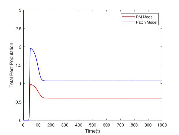
Figure 16. The time series figure showing the total pest population comparison of the system (8.1) and (3.1). The initial condition of the population for the patch model is [10,10,10,10], and that for the RM model is used as total pest and predator population, respectively, i.e. [10, 10].

We choose parameter sets for numerical simulations so that they adhere to the stability criteria of the equilibrium points in both systems. Here, the parameter set $k=1,\alpha=0.2,\xi=0.5,\epsilon_{1}=0.4,\epsilon_{2}=0.8,\delta_{1}=\delta_{2}=0.15,k_{2}=0.1,k_{4}=0.2$. In figure (15), we see that the overall pest population in a two-patch setting with additional food is lower than the RM model.

Figure (16), time series shows the comparison between RM-model and the new system under parameter set $k=1,\alpha=0.2,\xi=0.2,\epsilon_{1}=\epsilon_{2}=0.4,\delta_{1}=\delta_{2}=0.15,k_{1}=0,k_{2}=0.8,k_{3}=0,k_{4}=0.2.$ We validate lemma 10 by numerically validating it, as it can be seen that the total pest population in the classical model is lower than the patch model with some choice of $(\xi,k_{2})$. The model has the capability to have both a higher and lower total pest population than the RM model. The region corresponding to $\xi$ and $k_{2}$ can be broken down into different regions where for any fixed parameter set, there can be a choice of $(\xi,k_{2})$ for which we can have both higher or lower total pest population in the system under conditions given in lemma 9 and 10, as it can be seen in figure (17).

Figure (18), time series shows the comparison of interior equilibrium for both the system (3.1) and (8.1). We have seen numerically, under some parametric restrictions, (3.1) can exhibit a lower pest population than (8.1). In this comparison, the patch model’s total pest population is $x_{1}^{\star}+x_{2}^{\star}$, whereas the pest population in the Rosenzweig-MacArthur model is $x_{r}^{*}$.

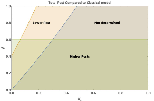
Figure 17. Comparison of total pest population: RM model vs. Patch model. For fixed parameters $(\xi,k_{2})$ are varied to see regions where the total pest population in the RM model differs from the Patch model. ”Lower Pest” means the Patch model has a lower pest population than the RM model and vice versa.

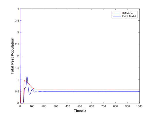
Figure 18. Comparison of total pest population: RM model vs. Patch model for interior equilibrium. Here, the parameters are $k=1,\alpha=0.2,\xi=0.37,\epsilon_{1}=\epsilon_{2}=0.4,\delta_{1}=\delta_{2}=0.15,k_{2}=0.1,k_{4}=0.2$. The initial condition of the pest population is $(2,2)$, and that for the RM model is $(2)$ with I.C. $=[2,2,2,2]$.

In the next section, we will compare the classical pest-predator additional food model and the two-patch additional food model to compare the total pest population density.

8.2. Classical two-species additional food model vs. Patch driven Additional food model

Secondly, we study classical Holling type II additional food model [41], which is given by

(8.2) $$\dot{x_{h}} =x_{h}\bigg{(}1-\dfrac{x_{h}}{k}\bigg{)}-\bigg{(}\dfrac{x_{h}y_{h}}{1+x_{h}+\alpha\xi}\bigg{)}$$

$$\dot{y_{h}} =\epsilon_{1}\bigg{(}\dfrac{x_{h}+\xi}{1+x_{h}+\alpha\xi}\bigg{)}y_{h}-\delta_{1}y_{h}$$

Interior equilibrium for $\eqref{org_model}$ are:

$$x_{h}^{*}=\dfrac{\delta_{1}+\xi(\alpha\delta_{1}-\epsilon_{1})}{(\epsilon_{1}-\delta_{1})},\hskip 5.69046pty_{h}^{*}=(1+x_{h}+\alpha\xi)(1-\dfrac{x_{h}}{k})$$

we are considering the case of boundary equilibrium $E_{2}=(0,y_{1}^{*},x_{2}^{*},y_{2}^{*})$ in (3.1), so total pest population in the system is $x_{2}$.

Lemma 11.

The system (3.1) can achieve lower pest population than system (8.2) if one of the following conditions holds,

If $\xi<\xi_{*}$ or ($\xi>\xi_{*})$

1. If $\tilde{A}>0$ then $\xi\in(\xi_{1},\xi_{2})$ or $\xi\in[0,\xi_{1})\cup(\xi_{2},1]$

2. If $\tilde{A}<0$ then $\xi\in[0,\xi_{1})\cup(\xi_{2},1]$ or $\xi\in(\xi_{1},\xi_{2})$

Proof.

We will compare the $(x_{h}^{*},y_{h}^{*})$ equilibrium of system (8.2) and the $(0,y_{1}^{*},x_{2}^{*},y_{2}^{*})$ equilibrium of system (3.1).

We know, $x_{h}^{*}=\dfrac{\delta_{1}+\xi(\alpha\delta_{1}-\epsilon_{1})}{(\epsilon_{1}-\delta_{1})},$ and $x_{2}^{*}=\dfrac{\tilde{Q}}{\epsilon_{2}-\tilde{Q}}$, where $\tilde{Q}=\delta_{2}+k_{4}+\dfrac{k_{2}\ k_{4}}{\dfrac{\epsilon_{1}\xi}{1+\alpha\xi}\ -\delta_{1}-k_{2}}.$

Thus, in order for the pest population to be lower in the system (3.1), we need

$\dfrac{\delta_{1}+\xi(\alpha\delta_{1}-\epsilon_{1})}{(\epsilon_{1}-\delta_{1})}>\dfrac{\tilde{Q}}{\epsilon_{2}-\tilde{Q}}$

When, $\epsilon_{2}-\tilde{Q}>0\text{ (required for the existence of $E_{2}$) }\implies\tilde{Q}\epsilon_{1}<\delta_{1}\epsilon_{2}+\xi\{(\epsilon_{2}-\tilde{Q})(\alpha\delta_{1}-\epsilon_{1})\}$

(8.3) $$\tilde{Q}\epsilon_{1}-\xi\tilde{Q}\epsilon_{1}+\xi\tilde{Q}\alpha\delta_{1}-\xi\alpha\epsilon_{2}\delta_{1}+\xi\epsilon_{1}\epsilon_{2}<\delta_{1}\epsilon_{2}$$

Putting the value $\tilde{Q}$ in the above equation,

1. If $\xi=\xi_{*}<\dfrac{\delta_{1}+k_{2}}{\epsilon_{1}-\alpha(\delta_{1}+k_{2})}$ then above equation becomes,

   $$\left(\epsilon_{1}\left(1-\xi\right)+\xi\alpha\delta_{1}\right)\left(\left(\delta_{2}+k_{4}\right)\dfrac{\epsilon_{1}\xi}{1+\alpha\xi}\right)-\delta_{1}\delta_{2}-k_{2}\delta_{2}-\delta_{1}k_{4}+\left(\dfrac{\epsilon_{1}\xi}{1+\alpha\xi}\ -\delta_{1}-k_{2}\right)\left(\xi\epsilon_{1}\epsilon_{2}-\xi\alpha\epsilon_{2}\delta_{1}-\delta_{1}\epsilon_{2}\right)>0$$

   $$\implies\left(1-\xi\right)\{\left(\delta_{2}+k_{4}\right)\epsilon_{1}^{2}\xi-\epsilon_{1}\left(1+\alpha\xi\right)\left(\delta_{1}\delta_{2}+k_{2}\delta_{2}+\delta_{1}k_{4}\right)\}$$

   $$\hskip 28.45274pt+\xi\hskip 2.84544pt\{\epsilon_{1}\xi\alpha\delta_{1}\left(\delta_{2}+k_{4}\right)-\alpha\delta_{1}\left(1+\alpha\xi\right)\left(\delta_{1}\delta_{2}+k_{2}\delta_{2}+\delta_{1}k_{4}\right)\}$$

   $$\implies\left(1-\xi\right)\{\left(\delta_{2}+k_{4}\right)\epsilon_{1}^{2}\xi-\epsilon_{1}\left(1+\alpha\xi\right)\left(\delta_{1}\delta_{2}+k_{2}\delta_{2}+\delta_{1}k_{4}\right)\}$$

   $$\hskip 28.45274pt+\xi\hskip 2.84544pt\{\epsilon_{1}\xi\alpha\delta_{1}\left(\delta_{2}+k_{4}\right)-\alpha\delta_{1}\left(1+\alpha\xi\right)\left(\delta_{1}\delta_{2}+k_{2}\delta_{2}+\delta_{1}k_{4}\right)\}$$

   $$\implies\xi^{2}\hskip 2.84544pt\{\left(\alpha\delta_{1}-\epsilon_{1}\right)\left(\epsilon_{1}\left(\delta_{2}+k_{4}\right)-\alpha\left(\delta_{1}\delta_{2}+k_{2}\delta_{2}+\delta_{1}k_{4}\right)+\alpha\epsilon_{2}\left(\delta_{1}+k_{2}\right)-\epsilon_{1}\epsilon_{2}\right)\}$$

   $$\hskip 28.45274pt+\xi\hskip 2.84544pt\{\epsilon_{1}^{2}\left(\delta_{2}+k_{4}\right)+\left(\delta_{1}\delta_{2}+k_{2}\delta_{2}+\delta_{1}k_{4}\right)\left(\epsilon_{1}-\alpha\epsilon_{1}-\alpha\delta_{1}\right)+\left(\delta_{1}+k_{2}\right)\left(\alpha\epsilon_{2}\delta_{1}-\epsilon_{1}\epsilon_{2}+\alpha\epsilon_{2}\delta_{1}\right)-\epsilon_{1}\epsilon_{2}\delta_{1}\}$$

   $$\hskip 28.45274pt+\delta_{1}\epsilon_{2}\left(\delta_{1}+k_{2}\right)-\epsilon_{1}\left(\delta_{1}\delta_{2}+k_{2}\delta_{2}+\delta_{1}k_{4}\right)>0$$

   The above equation can be written as:

   $$\tilde{A}\xi^{2}+\tilde{B}\xi+\tilde{C}>0$$

   where,

   $$\tilde{A} =\left(\alpha\delta_{1}-\epsilon_{1}\right)\left(\epsilon_{1}\left(\delta_{2}+k_{4}\right)-\alpha\left(\delta_{1}\delta_{2}+k_{2}\delta_{2}+\delta_{1}k_{4}\right)+\alpha\epsilon_{2}\left(\delta_{1}+k_{2}\right)-\epsilon_{1}\epsilon_{2}\right)$$

   $$\tilde{B} =\epsilon_{1}^{2}\left(\delta_{2}+k_{4}\right)+\left(\delta_{1}\delta_{2}+k_{2}\delta_{2}+\delta_{1}k_{4}\right)\left(\epsilon_{1}-\alpha\epsilon_{1}-\alpha\delta_{1}\right)+\left(\delta_{1}+k_{2}\right)\left(\alpha\epsilon_{2}\delta_{1}-\epsilon_{1}\epsilon_{2}+\alpha\epsilon_{2}\delta_{1}\right)-\epsilon_{1}\epsilon_{2}\delta_{1}$$

   $$\tilde{C} =\delta_{1}\epsilon_{2}\left(\delta_{1}+k_{2}\right)-\epsilon_{1}\left(\delta_{1}\delta_{2}+k_{2}\delta_{2}+\delta_{1}k_{4}\right)$$

   The roots are: $\xi_{1}=-\tilde{B}-\dfrac{\sqrt{\tilde{B}^{2}-4\tilde{A}\tilde{C}}}{2\tilde{A}}$ and, $\xi_{2}=-\tilde{B}+\dfrac{\sqrt{\tilde{B}^{2}-4\tilde{A}\tilde{C}}}{2\tilde{A}}$

   1. If $\tilde{D}=\tilde{B}^{2}-4\tilde{A}\tilde{C}>0,\tilde{A}>0$ then, $\xi<\xi_{1}$ or $\xi>\xi_{2}$

   2. If $\tilde{D}=\tilde{B}^{2}-4\tilde{A}\tilde{C}>0,\tilde{A}<0$ then, $\xi_{1}<\xi<\xi_{2}$

2. If $\xi=\xi_{*}>\dfrac{\delta_{1}+k_{2}}{\epsilon_{1}-\alpha(\delta_{1}+k_{2})}$ then the equation becomes,

$$\tilde{A}\xi^{2}+\tilde{B}\xi+\tilde{C}<0$$

where,

$\tilde{A}=\left(\alpha\delta_{1}-\epsilon_{1}\right)\left(\epsilon_{1}\left(\delta_{2}+k_{4}\right)-\alpha\left(\delta_{1}\delta_{2}+k_{2}\delta_{2}+\delta_{1}k_{4}\right)+\alpha\epsilon_{2}\left(\delta_{1}+k_{2}\right)-\epsilon_{1}\epsilon_{2}\right)$

$\tilde{B}=\epsilon_{1}^{2}\left(\delta_{2}+k_{4}\right)+\left(\delta_{1}\delta_{2}+k_{2}\delta_{2}+\delta_{1}k_{4}\right)\left(\epsilon_{1}-\alpha\epsilon_{1}-\alpha\delta_{1}\right)+\left(\delta_{1}+k_{2}\right)\left(\alpha\epsilon_{2}\delta_{1}-\epsilon_{1}\epsilon_{2}+\alpha\epsilon_{2}\delta_{1}\right)-\epsilon_{1}\epsilon_{2}\delta_{1}$

$\tilde{C}=\delta_{1}\epsilon_{2}\left(\delta_{1}+k_{2}\right)-\epsilon_{1}\left(\delta_{1}\delta_{2}+k_{2}\delta_{2}+\delta_{1}k_{4}\right)$

The roots are: $\xi_{1}=-\tilde{B}-\dfrac{\sqrt{\tilde{B}^{2}-4\tilde{A}\tilde{C}}}{2\tilde{A}}$ and, $\xi_{2}=-\tilde{B}+\dfrac{\sqrt{\tilde{B}^{2}-4\tilde{A}\tilde{C}}}{2\tilde{A}}$

1. If $\tilde{D}=\tilde{B}^{2}-4\tilde{A}\tilde{C}>0,\tilde{A}>0$ $\implies\xi_{1}<\xi<\xi_{2}$

2. If $\tilde{D}=\tilde{B}^{2}-4\tilde{A}\tilde{C}>0,\tilde{A}<0$ $\implies\xi<\xi_{1}$ or $\xi>\xi_{2}$

∎

We conducted a numerical investigation to compare the interior equilibrium between systems (3.1) and (8.2). Figure (19), demonstrates that, within certain parameter constraints, (3.1) can have a lower pest population than (8.2). In this comparison, the total pest population in the patch model is taken as $x_{1}^{\star}+x_{2}^{\star}$, whereas the pest population in the classical two-species additional food model is $x_{h}^{*}$.

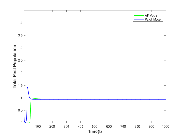
Figure 19. Comparison of total pest population: Classical two-species additional food model vs. Patch model for interior equilibrium. Here, the parameters are $k=1,\alpha=0.2,\xi=0.37,\epsilon_{1}=0.2,\epsilon_{2}=0.8,\delta_{1}=\delta_{2}=0.15,k_{2}=0.1,k_{4}=0.2$ with I.C. $=[2,2,2,2]$.

9. Discussion and conclusion

Motivated by recent innovative developments in landscape management, particularly in the mid-western US and the state of Iowa, such as the STRIPS program, we have presented a predator-pest bio-control for a two-patch system, with AF. Herein a predator is introduced into a “patch” such as a prairie strip or STRIP, which has AF. The AF boosts the predators efficacy, and it disperses into a second “patch”, which is a adjacent or neighboring crop field, to target a pest. To the best of our knowledge, such a study of the dynamics of a two-patch system with AF in one patch, has not been analyzed earlier. The effect of dispersal of the predator population between the patches has been studied extensively, and the biological implication of the results have also been analyzed. We have shown that linear (local) dispersal of the predator population between the patches can have an interesting dynamics on the stability of the equilibrium states.

As in section (4), it can be seen that linear predator dispersal between patches can help in blow-up prevention, see Figure (2(a)) and Figure (2(b)), which is prevalent in many AF models with pest dependent functional response [25]. Unlike earlier studies where a higher-order term like intra-specific predator competition, predator dependent function response, or group defense in the pest is required to prevent blow-up , an AF driven patch system can also lead to such prevention, solely with a linear dispersal term.

The stability of the equilibrium states has also been studied extensively, as they are of great importance for bio-control. It is observed that pest extinction is possible in either patch under certain parametric restrictions. In particular, pest extinction is possible in the crop field, where there are no predators present initially, see Figure (5). The predators are present/introduced only in the prairie strip, and move into the second patch, that is the crop field via dispersal.

The higher dimension of the model makes it unpragmatic to have a closed-form parametric value based expression for the equilibrium population, so numerical evidence is given to validate our quantitative studies. Total pest eradication from both patches is also possible but under strict parametric equality. This is highly unlikely from a biological point of view.

Furthermore, several other kinds of dynamics have been uncovered for the proposed model. It is sensitive to initial conditions and can give rise to stable limit cycles. The stable limit cycles occur due to a Hopf bifurcation, via which a stable interior equilibrium loses stability, resulting in the occurrence of a stable limit cycle. What is also seen is a further period doubling process which, under certain parametric windows, gives rise to chaotic dynamics. Chaos is studied numerically and validated by testing the Lyapunov coefficient. It is seen that for a fixed parameter set, some specific amount of additional food can give rise to chaotic behavior in the proposed model.

The benefits of the model as an effective bio-control tool are studied by comparing it with the classical Rosenzweig-MacArthur prey-predator model and the classical AF model with Holling Type II functional response. In each case, we compare the pest population density to conclude that the total pest population is lower in the two-patch AF system than in a classical predator-pest (essentially one-patch) system. In particular, the pest population in the AF patch driven system can be less than the pest population in the classical bio-control system, for several parameter sets where interior equilibrium is stable, for a choice of dispersal rate of predators.

In conclusion, an AF patch-driven prey-pest model can result in an effective bio-control strategy. The dispersal of the predator population between patches can result in pest extinction in certain patches - in particular, in our setting it can do so in the crop field, which is the main patch of interest as far as pest density goes. This essentially results in successful bio-control. Also, the patch model can keep the total prey population lower than in models without patch structure, thus having the benefit of checking the pest population using predator dispersal.

We note there are several open questions at this juncture. Both prey and predator population dispersal could be considered. Furthermore, non-linear or non-local dispersal, say akin to drift by strong winds, could be considered. Also, one can consider the spatially explicit patch model, where various shapes of the prairie strip could be modeled. This is part of the larger question of what shape/density of resource distribution is optimal. There is recent progress in these directions in spatial ecology, in the single species case [19, 20], but the question of this “optimality” in systems (such as in our setting) where the optimality would be measured in keeping pest density to minimum levels, remains open. Furthermore, one could consider explicit pest dynamics in the crop field, if one were attempting bio-control of certain specific target pests, such as the soybean aphid. In such a setting, depending on the type of host plant, resistant varieties or susceptible varieties, the dynamics of the pest could change [2]. Such considerations would be important in a bio-control context of the soybean aphid. Dynamics could also be affected by weather events such as drought or flood. This would affect both host plant quality and the herbivore dynamics.

All in all, many of these current and future approaches could result in interesting predator-pest dynamics. Field experiments are encouraged, which can show the power of patch structure as a bio-control strategy in agricultural practice today. These and related questions continue to be the subject of our current investigations.

10. Appendix

10.1. Proof of Lemma 1

Proof.

From the nullcline $\dot{y_{2}}=0$ we have,

(10.1) $$y_{2}^{*}=\frac{k_{4}}{\delta_{2}+k_{4}}\ y_{1}^{*}$$

Using the nullcline $\dot{x_{1}}=0$,

$$x_{1}^{*}\ \left\{\left(1-\frac{x_{1}^{*}}{k}\right)-\frac{y_{1}^{*}}{1+x_{1}^{*}+\alpha\xi}-\right\}=0$$

either $x_{1}^{*}=0$ or,

$$y_{1}^{*}=(1-\frac{x_{1}^{*}}{k})(1+x_{1}^{*}+\alpha\xi)$$

Hence,

(10.2) $$y_{1}^{*}=\left(1-\frac{x_{1}^{*}}{k}\right)\left(1+x_{1}^{*}+\alpha\xi\right)$$

Now, using the nullcline $\dot{y_{1}}=0$, and substituting the value of $y_{2}^{*}$ from (10.1) we have,

$$y_{1}^{*}\ \left\{\epsilon_{1}\left(\frac{x_{1}+\xi}{1+x_{1}+\alpha\xi}\right)-\delta_{1}-k_{2}+\frac{k_{2}k_{4}}{\delta_{2}+k_{4}}\right\}=0$$

$\therefore$ either $y_{1}^{*}=0$ or,

(10.3) $$\epsilon_{1}\left(\frac{x_{1}^{*}+\xi}{1+x_{1}^{*}+\alpha\xi}\right)-\delta_{1}-k_{2}+\frac{k_{2}k_{4}}{\delta_{2}+k_{4}}=0$$

simplifying (10.3) gives the expression of $x_{1}^{*}$ in terms of parameters,

(10.4) $$x_{1}^{*}=\frac{Q\ \left(1+\alpha\xi\right)-\epsilon_{1}\xi}{\epsilon_{1}-Q}$$

where $Q$ is defined by,

$$Q=\frac{\delta_{1}\delta_{2}+\delta_{1}k_{4}+k_{2}\delta_{2}}{\delta_{2}+k_{4}}$$

Thus, the equilibrium point $E_{1}=(x_{1}^{*},y_{1}^{*},0,y_{2}^{*})$ exists if $\xi<\dfrac{Q}{\epsilon_{1}-\alpha Q}$ and $\epsilon_{1}>Q$. ∎

10.2. Proof of Lemma 2

Proof.

Using the equation $\dot{y_{1}}=0$ then,

$$y_{1}^{*}\left[\epsilon_{1}\left(\frac{\xi}{1+\alpha\xi}\right)\ -\delta_{1}-k_{2}\right]+k_{2}\ y_{2}^{*}=0,$$

(10.5) $$y_{2}^{*}=\frac{-y_{1}^{*}}{k_{2}}\left[\epsilon_{1}\left(\frac{\xi}{1+\alpha\xi}\right)\ -\delta_{1}-k_{2}\right]$$

from $\dot{x_{2}}=0$,

$$x_{2}^{*}\left(1-\frac{x_{2}^{*}}{k}\right)-\frac{x_{2}^{*}y_{2}^{*}}{1+x_{2}^{*}}=0$$

either $x_{2}^{*}=0$ or

(10.6) $$y_{2}^{*}=\left(1-\frac{x_{2}^{*}}{k}\right)\left(1+x_{2}^{*}\right)$$

and from $\dot{y_{2}}=0$ then,

(10.7) $$y_{1}^{*}=\frac{-y_{2}^{*}}{k_{4}}\left[\epsilon_{2}\left(\frac{x_{2}^{*}}{1+x_{2}^{*}}\right)-\delta_{2}-k_{4}\right]$$

substituting the value of $y_{1}^{*}$ from (10.5),

$$y_{2}^{*}\left[k_{2}-\frac{1}{k_{4}}\left(\frac{\epsilon_{2}x_{2}^{*}}{1+x_{2}^{*}}-\delta_{2}-k_{4}\right)\left(\frac{\epsilon_{1}\xi}{1+\alpha\xi}\ -\delta_{1}-k_{2}\right)\right]=0$$

either $y_{2}^{*}=0$ or

$$\left[k_{2}-\dfrac{1}{k_{4}}\left(\dfrac{\epsilon_{2}x_{2}^{*}}{1+x_{2}^{*}}-\delta_{2}-k_{4}\right)\left(\dfrac{\epsilon_{1}\xi}{1+\alpha\xi}\ -\delta_{1}-k_{2}\right)\right]=0$$

which gives the value of $x_{2}^{*}$ in terms of parameters only,

(10.8) $$x_{2}^{*}=\dfrac{\tilde{Q}}{\epsilon_{2}-\tilde{Q}}$$

where $\tilde{Q}$ is define by,

$$\tilde{Q}=\delta_{2}+k_{4}+\dfrac{k_{2}\ k_{4}}{\left(\dfrac{\epsilon_{1}\xi}{1+\alpha\xi}\ -\delta_{1}-k_{2}\right)}$$

Thus, the equilibrium point $E_{2}=(0,y_{1}^{*},x_{2}^{*},y_{2}^{*})$ exists if $\epsilon_{2}-\tilde{Q}>0\ \&\ \tilde{Q}>0$ ∎

10.3. Proof of Lemma 3

Proof.

From the nullcline $\dot{y_{2}}=0$ we have,

(10.9) $$y_{2}^{*}=\dfrac{k_{4}}{\delta_{2}+k_{4}}\ y_{1}^{*}$$

and from $\dot{y_{1}}=0$,

$$y_{1}^{*}\left[\epsilon_{1}\left(\frac{\xi}{1+\alpha\xi}\right)\ -\delta_{1}-k_{2}\right]+k_{2}\ y_{2}^{*}=0,$$

Using the value of $y_{2}^{*}$ from (10.9),

$$y_{1}^{*}\left[\epsilon_{1}\left(\frac{\xi}{1+\alpha\xi}\right)\ -\delta_{1}-k_{2}+\dfrac{k_{2}k_{4}}{\delta_{2}+k_{4}}\right]=0,$$

either $y_{1}^{*}=0$ or,

(10.10) $$\left[\epsilon_{1}\left(\frac{\xi}{1+\alpha\xi}\right)\ -\delta_{1}-k_{2}+\dfrac{k_{2}k_{4}}{\delta_{2}+k_{4}}\right]=0$$

Simplifying (10.10) for $\xi$ gives,

$$\xi=\dfrac{{Q}}{\epsilon_{1}-\alpha{Q}}\text{ given,}\ \epsilon_{1}-\alpha{Q}>0$$

where ${Q}$ is defined by:

$$Q=\frac{\delta_{1}\delta_{2}+\delta_{1}k_{4}+k_{2}\delta_{2}}{\delta_{2}+k_{4}}$$

Therefore, the equilibrium point $E_{3}=(0,y_{1}^{*},0,y_{2}^{*})$ exists if $\xi=\dfrac{{Q}}{\epsilon_{1}-\alpha{Q}}$ and without additional food $E_{3}$ doesn’t exists. ∎

10.4. Proof of Lemma 4

Proof.

From the nullcline $\dot{x}_{1}=0$ either we have $x_{1}^{\star}=0$ or

(10.11) $$\hskip 5.69046pty_{1}^{\star}=\left(1-\frac{x_{1}^{\star}}{k}\right)\left(1+x_{1}^{\star}+\alpha\xi\right)$$

from $\dot{y}_{1}=0$

(10.12) $$y_{1}^{\star}\ \left\{\epsilon_{1}\left(\frac{x_{1}^{\star}+\xi}{1+x_{1}^{\star}+\alpha\xi}\right)-\delta_{1}-k_{2}\right\}+k_{2}y_{2}^{\star}=0$$

from $\dot{x}_{2}=0$ either $x_{2}^{\star}=0$ or

(10.13) $$y_{2}^{\star}=\left(1-\frac{x_{2}^{\star}}{k}\right)\left(1+x_{2}^{\star}\right)$$

and with $\dot{y_{2}}=0$ we have,

(10.14) $$y_{2}^{\star}\left[\epsilon_{2}\left(\frac{x_{2}^{\star}}{1+x_{2}^{\star}}\right)-\delta_{2}-k_{4}\right]+k_{4}y_{1}^{\star}=0$$

From $\eqref{int_eq_1}$ and $\eqref{int_eq_2}$ we have,

(10.15) $$y_{2}^{\star}=\frac{-\left(1-\dfrac{x_{1}^{\star}}{k}\right)}{k_{2}}\left\{\epsilon_{1}(x_{1}^{\star}+\xi)-(\delta_{1}+k_{2})(1+x_{1}^{\star}+\alpha\xi)\right\}$$

For $y_{2}^{\star}$ to exist, we have the condition on $x_{1}^{\star}$,

$$\epsilon_{1}(x_{1}^{\star}+\xi)<(\delta_{1}+k_{2})(1+x_{1}^{\star}+\alpha\xi)$$

if $\epsilon_{1}>\delta_{1}+k_{2}$ then,

$$x_{1}^{\star}<\frac{\delta_{1}+k_{2}}{\epsilon_{1}-(\delta_{1}+k_{2})}-\alpha\xi$$

From $\eqref{int_eq_3}$ and $\eqref{int_eq_4}$ we have,

(10.16) $$y_{1}^{\star}=\frac{-\left(1-\dfrac{x_{2}^{\star}}{k}\right)}{k_{4}}\left\{\epsilon_{2}x_{2}^{\star}-(\delta_{2}+k_{4})(1+x_{2}^{\star})\right\}$$

For $y_{1}^{\star}$ to exist, we have the condition on $x_{2}^{\star}$,

$$\epsilon_{2}x_{2}^{\star}<(\delta_{2}+k_{4})(1+x_{2}^{\star})$$

if $\epsilon_{2}>\delta_{2}+k_{4}$ then,

$$x_{2}^{\star}<\frac{\delta_{2}+k_{4}}{\epsilon_{2}-(\delta_{2}+k_{4})}$$

Using $\eqref{int_eq_1}$ and $\eqref{int_eq_6}$ after eliminating $y_{1}^{\star}$ we have,

(10.17) $$k_{4}\left(1-\frac{x_{1}^{\star}}{k}\right)\left(1+x_{1}^{\star}+\alpha\xi\right)=-(1-\dfrac{x_{2}^{\star}}{k})\left\{\epsilon_{2}x_{2}^{\star}-(\delta_{2}+k_{4})(1+x_{2}^{\star})\right\}$$

Using $\eqref{int_eq_3}$ and $\eqref{int_eq_5}$ after eliminating $y_{2}^{\star}$ we have,

(10.18) $$k_{2}\left(1-\frac{x_{2}^{\star}}{k}\right)\left(1+x_{2}^{\star}\right)=-\left(1-\dfrac{x_{1}^{\star}}{k}\right)\left\{\epsilon_{1}(x_{1}^{\star}+\xi)-(\delta_{1}+k_{2})(1+x_{1}^{\star}+\alpha\xi)\right\}$$

To find expression for $x_{2}^{\star}$, we equate $\eqref{x1_x2_implicit_eq_1}$ and $\eqref{x1_x2_implicit_eq_2}$ then,

(10.19) $$k_{2}k_{4}\left(1+x_{2}^{\star}\right)\left(1+x_{1}^{\star}+\alpha\xi\right)=\left\{\epsilon_{2}x_{2}^{\star}-(\delta_{2}+k_{4})(1+x_{2}^{\star})\right\}\left\{\epsilon_{1}(x_{1}^{\star}+\xi)-(\delta_{1}+k_{2})(1+x_{1}^{\star}+\alpha\xi)\right\}$$

$$\implies\dfrac{k_{2}k_{4}\left(1+x_{1}^{\star}+\alpha\xi\right)}{\left\{\epsilon_{1}(x_{1}^{\star}+\xi)-(\delta_{1}+k_{2})(1+x_{1}^{\star}+\alpha\xi)\right\}}=\dfrac{\left\{\epsilon_{2}x_{2}^{\star}-(\delta_{2}+k_{4})(1+x_{2}^{\star})\right\}}{\left(1+x_{2}^{\star}\right)}$$

$$\implies\dfrac{(\epsilon_{2}-(\delta_{2}+k_{4}))\left\{\epsilon_{1}(x_{1}^{\star}+\xi)-(\delta_{1}+k_{2})(1+x_{1}^{\star}+\alpha\xi)\right\}-k_{2}k_{4}\left(1+x_{1}^{\star}+\alpha\xi\right)}{\epsilon_{2}\left\{\epsilon_{1}(x_{1}^{\star}+\xi)-(\delta_{1}+k_{2})(1+x_{1}^{\star}+\alpha\xi)\right\}}=\dfrac{1}{1+x_{2}^{\star}}$$

$$x_{2}^{\star}=f(x_{1}^{\star})=\dfrac{\epsilon_{1}(\delta_{2}+k_{4})(x_{1}^{\star}+\xi)-(1+x_{1}^{\star}+\alpha\xi)(\delta_{1}\delta_{2}+k_{2}\delta_{2}+k_{4}\delta_{1})}{(\epsilon_{2}-(\delta_{2}+k_{4}))\left\{\epsilon_{1}(x_{1}^{\star}+\xi)-(\delta_{1}+k_{2})(1+x_{1}^{\star}+\alpha\xi)\right\}-k_{2}k_{4}\left(1+x_{1}^{\star}+\alpha\xi\right)}$$

The expression for $x_{1}^{\star}$ can be found by solving the four nullclines, (10.11), (10.12), (10.13) and, (10.14).

∎

References

• [1] VS Ananth and DKK Vamsi “Achieving minimum-time biological conservation and pest management for additional food provided predator–prey systems involving inhibitory effect: A qualitative investigation” In Acta Biotheoretica 70.1 Springer, 2022, pp. 5
• [2] Aniket Banerjee, Ivair Valmorbida, Matthew E O’Neal and Rana Parshad “Exploring the dynamics of virulent and avirulent aphids: A case for a ‘within plant’refuge” In Journal of economic entomology 115.1 Oxford University Press US, 2022, pp. 279–288
• [3] Faina S Berezovskaya, Baojun Song and Carlos Castillo-Chavez “Role of prey dispersal and refuges on predator-prey dynamics” In SIAM Journal on Applied Mathematics 70.6 SIAM, 2010, pp. 1821–1839
• [4] J Robert Britton, Ana Ruiz-Navarro, Hugo Verreycken and Fatima Amat-Trigo “Trophic consequences of introduced species: Comparative impacts of increased interspecific versus intraspecific competitive interactions” In Functional Ecology 32.2 Wiley Online Library, 2018, pp. 486–495
• [5] Chris Cosner and Yuan Lou “Does movement toward better environments always benefit a population?” In Journal of mathematical analysis and applications 277.2 Elsevier, 2003, pp. 489–503
• [6] Donald Lee DeAngelis, RA Goldstein and Robert V O’Neill “A model for tropic interaction” In Ecology 56.4 Wiley Online Library, 1975, pp. 881–892
• [7] Robert Devaney “An introduction to chaotic dynamical systems” CRC press, 2018
• [8] Ulf Dieckmann, Bob O’Hara and Wolfgang Weisser “The evolutionary ecology of dispersal” In Trends in Ecology & Evolution 14.3 Elsevier, 1999, pp. 88–90
• [9] Michael E Dorcas et al. “Severe mammal declines coincide with proliferation of invasive Burmese pythons in Everglades National Park” In Proceedings of the National Academy of Sciences 109.7 National Acad Sciences, 2012, pp. 2418–2422
• [10] Lenore Fahrig et al. “Farmlands with smaller crop fields have higher within-field biodiversity” In Agriculture, Ecosystems & Environment 200 Elsevier, 2015, pp. 219–234
• [11] Stephen A Gourley and Yang Kuang “Two-species competition with high dispersal: the winning strategy” In Math. Biosci. Eng 2.2, 2005, pp. 345–362
• [12] Nathan L Haan, Yajun Zhang and Douglas A Landis “Predicting landscape configuration effects on agricultural pest suppression” In Trends in ecology & evolution 35.2 Elsevier, 2020, pp. 175–186
• [13] Karin M Kettenring and Carrie Reinhardt Adams “Lessons learned from invasive plant control experiments: a systematic review and meta-analysis” In Journal of applied ecology 48.4 Wiley Online Library, 2011, pp. 970–979
• [14] Mark Kot “Elements of mathematical ecology” Cambridge University Press, 2001
• [15] Claire Kremen and Adina M Merenlender “Landscapes that work for biodiversity and people” In Science 362.6412 American Association for the Advancement of Science, 2018, pp. eaau6020
• [16] Dinesh Kumar and Siddhartha P Chakrabarty “A comparative study of bioeconomic ratio-dependent predator–prey model with and without additional food to predators” In Nonlinear Dynamics 80 Springer, 2015, pp. 23–38
• [17] Dinesh Kumar and Siddhartha P Chakrabarty “A predator–prey model with additional food supply to predators: dynamics and applications” In Computational and Applied Mathematics 37 Springer, 2018, pp. 763–784
• [18] Wei-Min Liu “Criterion of Hopf bifurcations without using eigenvalues” In Journal of Mathematical Analysis and Applications 182.1 Elsevier, 1994, pp. 250–256
• [19] Idriss Mazari and Domènec Ruiz-Balet “A fragmentation phenomenon for a nonenergetic optimal control problem: Optimization of the total population size in logistic diffusive models” In SIAM Journal on Applied Mathematics 81.1 SIAM, 2021, pp. 153–172
• [20] Idriss Mazari and Domènec Ruiz-Balet “Spatial ecology, optimal control and game theoretical fishing problems” In Journal of Mathematical Biology 85.5 Springer, 2022, pp. 55
• [21] James Dickson Murray and James Dickson Murray “Mathematical Biology: II: Spatial Models and Biomedical Applications” Springer, 2003
• [22] Matthew E O’Neal, Adam J Varenhorst and Matthew C Kaiser “Rapid evolution to host plant resistance by an invasive herbivore: soybean aphid (Aphis glycines) virulence in North America to aphid resistant cultivars” In Current opinion in insect science 26 Elsevier, 2018, pp. 1–7
• [23] Dean R Paini et al. “Global threat to agriculture from invasive species” In Proceedings of the National Academy of Sciences 113.27 National Acad Sciences, 2016, pp. 7575–7579
• [24] Rana D Parshad, Sureni Wickramsooriya and Susan Bailey “A remark on “Biological control through provision of additional food to predators: A theoretical study”[Theor. Popul. Biol. 72 (2007) 111–120]” In Theoretical population biology 132 Elsevier, 2020, pp. 60–68
• [25] Rana D Parshad, Sureni Wickramasooriya, Kwadwo Antwi-Fordjour and Aniket Banerjee “Additional food causes predators to explode—unless the predators compete” In International Journal of Bifurcation and Chaos 33.03 World Scientific, 2023, pp. 2350034
• [26] Rana D Parshad, Emmanuel Quansah, Kelly Black and Matthew Beauregard “Biological control via “ecological” damping: an approach that attenuates non-target effects” In Mathematical biosciences 273 Elsevier, 2016, pp. 23–44
• [27] David Pimentel “Environmental and economic costs of the application of pesticides primarily in the United States” In Environment, development and sustainability 7 Springer, 2005, pp. 229–252
• [28] David Pimentel, Rodolfo Zuniga and Doug Morrison “Update on the environmental and economic costs associated with alien-invasive species in the United States” In Ecological economics 52.3 Elsevier, 2005, pp. 273–288
• [29] BSRV Prasad, Malay Banerjee and PDN Srinivasu “Dynamics of additional food provided predator–prey system with mutually interfering predators” In Mathematical biosciences 246.1 Elsevier, 2013, pp. 176–190
• [30] BSRV Prasad, Malay Banerjee and PDN Srinivasu “Dynamics of additional food provided predator–prey system with mutually interfering predators” In Mathematical biosciences 246.1 Elsevier, 2013, pp. 176–190
• [31] Maurice W Sabelis and Paul CJ Van Rijn “When does alternative food promote biological pest control?” In IOBC WPRS BULLETIN 29.4 IOBC/WPRS; 1998, 2006, pp. 195
• [32] Thomas W Sappington “Emerging issues in integrated pest management implementation and adoption in the North Central USA” In Integrated Pest Management: Experiences with Implementation, Global Overview, Vol. 4 Springer, 2014, pp. 65–97
• [33] Lisa A Schulte, Anna L MacDonald, Jarad B Niemi and Matthew J Helmers “Prairie strips as a mechanism to promote land sharing by birds in industrial agricultural landscapes” In Agriculture, Ecosystems & Environment 220 Elsevier, 2016, pp. 55–63
• [34] Lisa A Schulte et al. “Prairie strips improve biodiversity and the delivery of multiple ecosystem services from corn–soybean croplands” In Proceedings of the National Academy of Sciences 114.42 National Acad Sciences, 2017, pp. 11247–11252
• [35] Hanno Seebens et al. “No saturation in the accumulation of alien species worldwide” In Nature communications 8.1 Nature Publishing Group UK London, 2017, pp. 14435
• [36] Clélia Sirami et al. “Increasing crop heterogeneity enhances multitrophic diversity across agricultural regions” In Proceedings of the National Academy of Sciences 116.33 National Acad Sciences, 2019, pp. 16442–16447
• [37] HL Smith “The Rosenzweig-Macarthur predator-prey model” In School of Mathematical and Statistical Sciences, Arizona State University: Phoenix, 2008
• [38] William E Snyder and David H Wise “Predator interference and the establishment of generalist predator populations for biocontrol” In Biological Control 15.3 Elsevier, 1999, pp. 283–292
• [39] PDN Srinivasu and BSRV Prasad “Role of quantity of additional food to predators as a control in predator–prey systems with relevance to pest management and biological conservation” In Bulletin of mathematical biology 73.10 Springer, 2011, pp. 2249–2276
• [40] PDN Srinivasu and BSRV Prasad “Time optimal control of an additional food provided predator–prey system with applications to pest management and biological conservation” In Journal of mathematical biology 60.4 Springer, 2010, pp. 591–613
• [41] PDN Srinivasu, BSRV Prasad and M Venkatesulu “Biological control through provision of additional food to predators: a theoretical study” In Theoretical Population Biology 72.1 Elsevier, 2007, pp. 111–120
• [42] PDN Srinivasu, DKK Vamsi and I Aditya “Biological conservation of living systems by providing additional food supplements in the presence of inhibitory effect: a theoretical study using predator–prey models” In Differential Equations and Dynamical Systems 26 Springer, 2018, pp. 213–246
• [43] PDN Srinivasu, DKK Vamsi and VS Ananth “Additional food supplements as a tool for biological conservation of predator-prey systems involving type III functional response: A qualitative and quantitative investigation” In Journal of theoretical biology 455 Elsevier, 2018, pp. 303–318
• [44] Alejandro Tena et al. “Sugar provisioning maximizes the biocontrol service of parasitoids” In Journal of Applied Ecology 52.3 Wiley Online Library, 2015, pp. 795–804
• [45] Daniel H Thornton, Lyn C Branch and Melvin E Sunquist “The influence of landscape, patch, and within-patch factors on species presence and abundance: a review of focal patch studies” In Landscape Ecology 26 Springer, 2011, pp. 7–18
• [46] Mark C Urban, Ben L Phillips, David K Skelly and Richard Shine “A toad more traveled: the heterogeneous invasion dynamics of cane toads in Australia” In The American Naturalist 171.3 The University of Chicago Press, 2008, pp. E134–E148
• [47] Roy G Van Driesche, Thomas S Bellows, Roy G Van Driesche and Thomas S Bellows “Pest origins, pesticides, and the history of biological control” In Biological Control Springer, 1996, pp. 3–20
• [48] Edward Vasquez, Roger Sheley and Tony Svejcar “Creating invasion resistant soils via nitrogen management” In Invasive Plant Science and Management 1.3 Cambridge University Press, 2008, pp. 304–314
• [49] Sureni D Wickramsooriya, Aniket Banerjee, Jonathan Martin and Rana D. Parshad “Novel dynamics in an additional food provided predator-prey system with mutual interference” In Under Review, 2023
• [50] Jianguo Wu and Orie L Loucks “From balance of nature to hierarchical patch dynamics: a paradigm shift in ecology” In The Quarterly review of biology 70.4 University of Chicago Press, 1995, pp. 439–466