RCHEP/23-004 CERN-TH-2023-199

Confinement from Distance in Metric Space and its Relation to Cosmological Constant

$\text{Amineh Mohseni}^{a,b,}~{}\text{, Mahdi Torabian}^{a,c,}$

^aCenter for High Energy Physics, Department of Physics, Sharif University of Technology, Tehran, Iran

^bCERN, Theoretical Physics Department, 1211 Meyrin, Switzerland

^cPerimeter Institute for Theoretical Physics, Waterloo, ON, N2L 2Y5, Canada

We argue that, in a theory of quantum gravity, the gauge coupling and the confinement scale of a gauge theory are related to distance in the space of metric configurations, and in turn to the cosmological constant. To support the argument, we compute the gauge kinetic functions in variuos supersymmetric Heterotic and type II string compactifications and show that they depend on distance. According to the swampland program, the distance between two (anti) de Sitter vacua in the space of metric configurations is proportional to the logarithm of the ratio of cosmological constants and thus the confinement scale depends on the value of the cosmological constant. In this framework, for de Sitter space, we revisit the swampland Festina Lente bound and gauge theories in the dark dimension scenario. We show that if the Festina Lente bound is realized in a de Sitter vacuum and dependence on distance is strong enough, it will be realized in vacua with higher cosmological constants. In dark dimension scenario, as the value of cosmological constant is related to the decompactifying dimension, we find that the confinement scale is indeed related to radius of dark dimension. We show that in this scenario the Festina Lente bound holds for the standard model QCD, as well as all confining gauge groups with $N_{c}\lesssim 10^{3}$.

1 Introduction

The swampland program puts forward the idea that not all self-consistent low energy effective theories (EFTs) can be UV completed in a theory of quantum gravity. Its goal is to determine the set of conditions an EFT consistent with quantum gravity must satisfy [1, 2]. These criteria are formulated as conjectures with different levels of rigorousness (see [3, 4, 5, 6] for review). The swampland program provides guidelines for low energy physics, leads to explaining the properties of the observed universe and genuine predictions. It explains properties of low energy physics and in particular the value of low energy parameters which may otherwise seem unnatural (i.e. the Higgs mass parameter and the cosmological constant) [7, 8, 9, 10].

Among well-established conjectures are no global symmetries [11], the swampland distance conjecture (SDC) [12] and weak gravity conjecture (WGC) [13] which constitute core of the swampland program. These conjectures are not very predictive for low energy physics though. However, recently proposed conjectures including the swampland de Sitter conjecture [14, 15], the trans-Planckian censorship conjecture (TCC) [16] and the Festina Lente (FL) bound [18, 17] have direct implications for the low energy EFT. An interesting observation is that the swampland conjectures are related to each other. It suggests that they might be different aspects of quantum gravity principles and thus it is important, in the swampland program, to find out how different conjectures are related. Specially, connections between the predictive conjectures and the well-established ones would be interesting.

Yang-Mills gauge theories, characterized by a gauge group and a coupling constant, are indispensable parts of our description of low energy physics. In the framework of quantum field theory, the dimensionless gauge coupling in four dimensions is replaced by a confinement scale via dimensional transmutation. In the light of swampland program, it is interesting to study the confinement dynamics in a theory consistent with quantum gravity. The FL bound, motivated by studying black holes in dS space, puts a lower bound on mass of charged particles in dS space. In particular, it implies that a non-Abelian gauge theory in dS space must be either confined (at a scale higher or equal to the Hubble scale) or Higgsed. This condition is fulfilled in the Standard Model sector in the present dS phase of the universe; the electroweak symmetry is spontaneously broken and QCD is confined. However, in the absence of other dynamics, the FL bound becomes a non-trivial constraint in a dS phase with a higher cosmological constant e.g. during primordial inflation. In fact, the FL bound in different dS vacua is respected if the confinement scale increases as the cosmological constant increases.

In this paper, to examine the above possibility, we study the connection between the confinement scale of a gauge theory and the SDC. According to the generalized distance conjecture, the distance between vacua whose metrics are related by a Weyl transformation is the Weyl factor up to an order one constant [19]. We refer to it as distance in the space of metric configurations in the rest of the paper. We study the dependence of the gauge coupling on distance in the space of metric configurations and its implications for the confinement scale. To be specific, we study semi-realistic compactifications of heterotic, type IIA, and type IIB string theories in which we can compute the gauge kinetic functions in four dimensions. We find that the gauge coupling actually depends on distance in the space of metric configurations which consequently implies a distance dependent confinement scale. We expand the gauge kinetic function for small changes of distance so that we can draw general conclusions regardless of the exact form of the distance dependence. For (Anti) dS space, distance in the space of metric configurations is proportional to the logarithm of the cosmological constant. Therefore, our result implies that the confinement scale of a Yang-Mills theory depends on the cosmological constant. We find the condition that the FL bound is respected in all dS space with different vacuum energy. Furthermore, the arguments establish a relation between the SDC and the FL bound. Interestingly, our result is generic and is independent of the exact form of the scalar potential in the EFT or the details of moduli stabilization. Although the computable examples of compactifications we used are supersymmetric, we make general predictions which is believed to be held in non-supersymmetric constructions. The bottomline is that stringy effects are stronger that running due to loop effects.

Moreover, we study the distance dependent confinement scale and the FL bound in the dark dimension scenario which ties the dS space with small cosmological constant to decompactification of one extra dimension [10]. It is motivated by the observation of a tiny cosmological constant which indicates our universe sits in asymptotic limit of moduli space. In this scenario, the vacuum energy is sourced by the zero-point energy of lightest Kaluza-Klein modes and the Standard Model fields are localised on a brane perpendicular to the dark dimension. We study F-theory realization of this scenario with generic $CY_{4}$ compactification and GUT $D_{7}$ brane. In this setup we find that the gauge decreases (equivalently the confinement scale increases) as the radius of dark dimension decreases (i.e. cosmological constant increases). It is in agreement with the FL bound for confining gauge theories.

The structure of the paper is as follows; in section 2 we generally study a gauge theory with distance-dependent gauge kinetic function and derive the confinement scale as a function of distance in the metric space. We present examples of string theory compactifications to four dimensions. In section 3 we look into the implications of distance-dependent gauge coupling and the confinement scale in the (A)dS space and we find the condition that the FL bound is realized in all dS vacua. We also look at the dark dimension scenario for dS space with positive vacuum energy show that how the FL bound is respected in this scenario. Finally, we conclude in section 4.

2 Distance-Dependent Confinement Scale

According to generalised distance conjecture a distance can be associated to any dynamical field $\mathcal{O}_{I_{1},\dots I_{n}}$ as

$$\Delta_{\mathcal{O}}=\int\left(K^{I_{1},\dots I_{n},J_{1},\dots J_{n}}\,\frac{\partial\mathcal{O}_{I_{1},\dots I_{n}}}{\partial\tau}\frac{\partial\mathcal{O}_{J_{1},\dots J_{n}}}{\partial\tau}\right)^{\nicefrac{{1}}{{2}}}d\tau,$$ (1)

where $K$ is the metric in field space of $\mathcal{O}$, and $\tau$ parameterizes the geodesic path in field space. In particular, it is conjectured that the distance between vacua (or geometries) whose metrics are related via the following external Weyl transformation

$$\tilde{g}_{\mu\nu}=e^{2\Phi}g_{\mu\nu},$$ (2)

is given by field $\Phi$ (the Weyl factor) up to an order one constant, k, namely

$$\Delta=k\,\Phi,$$ (3)

it is proposed that taking all the contributions into account, the constant is fixed such that distance is positive [19].

In this paper we argue that due to quantum gravity effects the gauge kinetic function of a Yang-Mills theory typically depends on distance in the space of metric configurations, $\Phi$. To support our argument, in the next section, we present examples from string theory. In this section, we study the effect of this dependence on the confinement scale of a Yang-Mills theory given the action

$$\mathcal{L}_{\text{YM}} = -\frac{1}{4}f(\Phi)\,{\rm tr}\,(F_{\mu\nu}F^{\mu\nu}),$$ (4)

where $\Phi$ measures distance between vacua in the space of metric configurations. If we move in the space of metric configurations from a point where the UV (string scale) gauge coupling is $g_{0,\rm UV}$ (call it $\Phi=0$), the gauge coupling at a point at distance $\Phi$ from the initial point would be

$$g_{\rm UV}^{-2}=g_{0,\rm UV}^{-2}+[f(\Phi)-f(0)].$$ (5)

Furthermore, the gauge coupling runs with energy due to radiative corrections. Therefore, the gauge couplings in two vacua in the IR are related as

$$\alpha_{\rm IR}(\Phi,\mu)^{-1}=\alpha_{\rm IR}(0,\mu_{0})^{-1}+\frac{\beta_{0}}{4\pi}\ln\frac{\mu^{2}}{\mu_{0}^{2}}+4\pi[f(\Phi)-f(0)],$$ (6)

where $\alpha_{\rm IR}\equiv\frac{g_{\rm IR}^{2}}{4\pi}$ and $\beta_{0}$ is one-loop beta coefficient (for tha sake of simplicity, we assume that two theories in each vacuum we are comparing have similar field contents). If the gauge theory confines at $\mu_{\text{conf}}(0)$ when $\Phi=0$, then, at distance $\Phi$ away from that point the confinement scale would be

$$\mu_{\text{conf}}(\Phi)=\mu_{\text{conf}}(0)\,e^{-\frac{8\pi^{2}}{\beta_{0}}[f(\Phi)-f(0)]},$$ (7)

thus the confinement scale has a distance dependence induced by the gauge kinetic function.

Our goal is to make a general arguments from this observation regardless of the exact form of the gauge kinetic function or underlying dynamics of moduli stabilization. This can be done if we consider small changes in distance and consider the leading order expansion of the gauge kinetic function given $|\Phi|<1$ as

$$f\simeq f|_{\Phi=0}+\left(\partial_{\Phi}f\right)|_{\Phi=0}\Phi\equiv g_{0,\rm UV}^{-2}(1+r\Phi),$$ (8)

where $f|_{\Phi=0}=g_{0,\rm UV}^{-2}$ is the UV (string scale) gauge coupling at $\Phi=0$ and $r$ is defined as

$$r=\frac{\left(\partial_{\Phi}f\right)|_{\Phi=0}}{f|_{\Phi=0}},$$ (9)

we drop the UV index in the rest of the paper. Then, including the loop effects, confinement scale as a function of distance is

$$\mu_{\text{conf}}(\Phi)=\mu_{\text{conf}}(0)\,e^{-\frac{8\pi^{2}}{g_{0}^{2}\beta_{0}}r\Phi}.$$ (10)

For non-zero positive or negative $r$, the gauge coupling respectively decreases or increases as distance in metric space increases.

2.1 Evidence from String Theory

In this section, to support our argument, we present examples of four dimensional compactifications of string theory where gauge couplings depend on distance in the space of metric configurations. In particular, we study compactifications of the heterotic, type IIA, type IIB with $D7$/$D3$ branes and type IIB with $D9/D5$ branes (type I) to four dimensions.

The (relevant part of) string frame action after compactification to four dimensions is

$$S\supset\frac{1}{2\alpha^{\prime}}\int d^{4}x\sqrt{-G^{s}}\,e^{-2\phi_{4}}\left(R^{s}+\Lambda^{s}\right),$$ (11)

where $\phi_{4}$ is the four dimensional dilaton, which is a function of the ten-dimensional dilaton and the compactification volume ${\cal V}$

$$\phi_{4}=\phi-\frac{1}{2}\ln\left({\cal V}/\alpha^{\prime\,3}\right).$$ (12)

We consider two vacua in the space of metric configurations which are distinguished with their string frame metrics $G^{s,(1)}_{\mu\nu}$ and $G^{s,(0)}_{\mu\nu}$, and their four dimensional dilaton $\phi_{4}^{(1)}$ and $\phi_{4}^{(0)}$. As we eventually apply our result to (A)dS background, we consider metrics that differ by a Weyl transformation as

$$G_{\mu\nu}^{s,(1)}=e^{-2\omega}G_{\mu\nu}^{s,(0)},$$ (13)

where $\omega$ is in general, a function of ten dimensional dilaton and volume moduli.

The action can be written in the Einstein frame through a Weyl transformation of the metric

$$g^{E,(i)}_{\mu\nu}=e^{-2(\phi^{(i)}_{4}-c^{(i)})}G^{s,(i)}_{\mu\nu},$$ (14)

where $i=0,1$ and $c^{i}$ is a constant. We fix the Einstein frame by choosing $c^{(0)}=c^{(1)}=-\nicefrac{{1}}{{2}}\ln(2\alpha^{\prime})$ which sets the four dimensional Planck mass to one ($m_{{\rm Pl},4}=1$) at both points in metric space. It guarantees that we have removed Weyl redefinition without physical meaning given by $c^{(0)}\neq c^{(1)}$. Then, the External metrics of the two vacua we compare are related through the following Weyl transformation in Einstein frame

$$g^{E,(1)}_{\mu\nu}=e^{-2(\phi_{4}^{(1)}-\phi_{4}^{(0)}+\omega)}g^{E,(0)}_{\mu\nu},$$ (15)

Moreover, the cosmological constants are related as

$$\Lambda^{(1)}=e^{2(\phi_{4}^{(1)}-\phi_{4}^{(0)}+\omega)}\Lambda^{(0)}.$$ (16)

Finally, according to generalized distance conjecture, the distance between these vacua is given by

$$\Phi=-(\phi_{4}^{(1)}-\phi_{4}^{(0)}+\omega),$$ (17)

up to an order one constant.

The gauge kinetic function of a Yang-Mills theory obtained from string compactifications to four dimensions typically depends on field $\Phi$ through its dependence on volume and ten-dimensional dilaton. In fact, we show that $\partial_{\Phi}f\neq 0$ by computing

$$\partial_{\Phi}f=\sum_{i}\frac{\partial f}{\partial\rho_{i}}\frac{\partial\rho_{i}}{\partial\Phi}+\frac{\partial f}{\partial\phi}\frac{\partial\phi}{\partial\Phi},$$ (18)

where $\rho_{i}$ are the geometric moduli of the compact manifold and $\phi$ is the dilaton. The partial derivatives $\nicefrac{{\partial\rho_{i}}}{{\partial\Phi}}$ and $\nicefrac{{\partial\phi}}{{\partial\Phi}}$ tell us how moduli $\rho_{i},\phi$ change (through tunneling or rolling). These derivatives are determined by the structure of vacua or dynamics of the underlying quantum gravity theory, and account for the change of $\Phi$.

For the sake of concreteness, we study compactification on factorizable $T^{6}$ which allows explicit calculations. Although toroidal compactification is supersymmetric, we expect that our main point which is dependence of the gauge kinetic function on volume moduli and ten dimensional dilaton and therefore distance between vacua, holds also for compactification on more general manifolds. For factorizable $T^{6}$, equation (18) is computed as

$$\partial_{\Phi}f = \sum_{i=1}^{3}\frac{\partial f}{\partial R_{x}^{i}}\frac{\partial R_{x}^{i}}{\partial\Phi}+\sum_{i=1}^{3}\frac{\partial f}{\partial R_{y}^{i}}\frac{\partial R_{y}^{i}}{\partial\Phi}+\frac{\partial f}{\partial\phi}\frac{\partial\phi}{\partial\Phi},$$ (19)

where $R_{x}^{i}$ and $R_{y}^{i}$ are dimensionless radii in units of $\alpha^{\prime}$.

In order to compute the above constrained partial derivative, we parameterize change of the radii and the ten dimensional dilaton in the following way; such that $g_{i}$ contain information on how the geometric moduli change due to dynamics (tunneling or rolling) of the underlying theory

$${\rm d}R_{x}^{i}\equiv g^{i}_{x}{\rm d}\Phi,$$ (20)

$${\rm d}R_{y}^{i}\equiv g^{i}_{y}{\rm d}\Phi,$$ (21)

$${\rm d}\phi\equiv g_{\phi}{\rm d}\Phi,$$ (22)

change of different moduli accounts for the change of distance, that is the dynamics is subject to the constraint

$$\Phi=-(\phi_{4}-\phi_{4}^{0}+\omega),$$ (23)

where $\omega$ is a function of the ten dimensional dilaton and the geometric moduli, $\omega(R_{x}^{i},R_{y}^{i},\phi)$, and the four dimensional dilaton in terms of geometric data is

$$\phi_{4}=\phi-\frac{1}{2}\ln\big(\prod_{i=1}^{3}R_{x}^{i}R_{y}^{i}\big{missing}).$$ (24)

Upon differentiating, the above constraint implies

$$g_{\phi}=\frac{1}{2}\frac{1}{1+\frac{\partial\omega}{\partial\phi}}\Big{[}\sum_{i=1}^{3}\frac{g^{i}_{x}}{R_{x}^{i}}\Big{(}1-2\frac{\partial\omega}{\partial R_{x}^{i}}R_{x}^{i}\Big{)}+\sum_{i=1}^{3}\frac{g^{i}_{y}}{R_{y}^{i}}\Big{(}1-2\frac{\partial\omega}{\partial R_{y}^{i}}R_{y}^{i}\Big{)}-2\Big{]}.\quad$$ (25)

The derivatives $\nicefrac{{\partial\omega}}{{\partial R_{x}^{i}}},\nicefrac{{\partial\omega}}{{\partial R_{y}^{i}}},\nicefrac{{\partial\omega}}{{\partial\phi}}$ contain information on details of the compactification, which we leave as general functions. Substituting the above relation for $g_{\phi}$ in (19), we get

$$\partial_{\Phi}f = \sum_{i=1}^{3}\left(\frac{\partial f}{\partial R_{x}^{i}}+\frac{1}{2R_{x}^{i}}\frac{1-2\frac{\partial\omega}{\partial R_{x}^{i}}R_{x}^{i}}{1+\frac{\partial\omega}{\partial\phi}}\frac{\partial f}{\partial\phi}\right)g^{i}_{x}$$ (26)

$$+ \sum_{i=1}^{3}\left(\frac{\partial f}{\partial R_{y}^{i}}+\frac{1}{2R_{y}^{i}}\frac{1-2\frac{\partial\omega}{\partial R_{y}^{i}}R_{y}^{i}}{1+\frac{\partial\omega}{\partial\phi}}\frac{\partial f}{\partial\phi}\right)g^{i}_{y}$$ (27)

$$- \frac{1}{1+\frac{\partial\omega}{\partial\phi}}\frac{\partial f}{\partial\phi},$$ (28)

the ratio of expansion coefficients is then straightforwardly calculated according to (9). The properties of the structure of vacua or dynamics of the underlying theory is captured by $r$

2.1.1 Heterotic String Compactifications

Consider the low energy effective theory for compactifications of heterotic string. Symmetry arguments, [20], imply that gauge kinetic function of gauge fields in the effective four dimensional theory is as follows

$$f_{ab}=S\delta_{ab},$$ (29)

$$S=e^{-2\phi_{4}}+ia,$$ (30)

ratio of the expansion coefficients, which is a measure of distance dependence is

$$r_{\text{het}}=\frac{1}{1+\frac{\partial\omega}{\partial\phi}}\Big{[}2+\sum_{i=1}^{3}\frac{g_{x}^{i}}{R_{x}^{i}}\Big{(}\frac{\partial\omega}{\partial\phi}+2R_{x}^{i}\frac{\partial\omega}{\partial R_{x}^{i}}\Big{)}+\sum_{i=1}^{3}\frac{g_{y}^{i}}{R_{y}^{i}}\Big{(}\frac{\partial\omega}{\partial\phi}+2R_{y}^{i}\frac{\partial\omega}{\partial R_{y}^{i}}\Big{)}\Big{]},$$ (31)

where the radii and derivatives are evaluated at the expansion point. We note that $r_{\text{het}}$ captures the parameters $g_{x}^{i},g_{y}^{i}$ which contain information on how the geometric moduli change, also derivatives of the function $\omega$ that contain information about the details of the compactification, and the vacuum. This is also the case for type II examples that we investigate bellow.

2.1.2 Type II Compactifications

The gauge coupling of the gauge symmetry resulting from a stack of D-branes in type II compactifications follows from expanding the DBI action to quadratic order in gauge field strength. For $D_{p}$ brane the gauge coupling is as follows

$$f_{p}=e^{-\phi}\frac{\alpha^{\prime\,\nicefrac{{(3-p)}}{{2}}}}{(2\pi)^{p-2}}\text{Vol}(\Pi_{p-3}),$$ (32)

where $f_{p}\equiv\nicefrac{{1}}{{g_{p}^{2}}}$, $\text{Vol}(\Pi_{p-3})$ is volume of the cycle wrapped by the brane, and $\phi$ is the ten dimensional dilaton. The gauge coupling (32) has been calculated in terms of geometric data for compactification on a factorizable $T^{6}$ in [21].

Firstly, we consider type IIA with D6 branes. The gauge kinetic function is

$$f_{6}=\frac{e^{-\phi}}{2\pi}\prod_{i=1}^{3}\left(n_{i}^{2}R_{x}^{i\,2}+m_{i}^{2}R_{y}^{i\,2}\right)^{\nicefrac{{1}}{{2}}},$$ (33)

where $(m_{i},n_{i})$ are the wrapping numbers. The ratio of expansion coefficients is

$$r_{6}=\frac{1}{1+\frac{\partial\omega}{\partial\phi}}\Big{[}1\!\!\!\! + \!\!\!\frac{\partial\omega}{\partial\phi}\sum_{i=1}^{3}\frac{n_{i}^{2}g_{x}^{i}R_{x}^{i}+m_{i}^{2}g_{y}^{i}R_{y}^{i}}{n_{i}^{2}(R_{x}^{i})^{2}+m_{i}^{2}(R_{y}^{i})^{2}}$$ (34)

$$+ \!\!\!\frac{1}{2}\sum_{i=1}^{3}\frac{g_{x}^{i}}{R_{x}^{i}}\frac{n_{i}^{2}(R_{x}^{i})^{2}(1+2R_{x}^{i}\frac{\partial\omega}{\partial R_{x}^{i}})-m_{i}^{2}(R_{y}^{i})^{2}(1-2R_{x}^{i}\frac{\partial\omega}{\partial R_{x}^{i}})}{n_{i}^{2}(R_{x}^{i})^{2}+m_{i}^{2}(R_{y}^{i})^{2}}$$

$$+ \!\!\!\frac{1}{2}\sum_{i=1}^{3}\frac{g_{y}^{i}}{R_{y}^{i}}\frac{m_{i}^{2}(R_{y}^{i})^{2}(1+2R_{y}^{i}\frac{\partial\omega}{\partial R_{y}^{i}})-n_{i}^{2}(R_{x}^{i})^{2}(1-2R_{y}^{i}\frac{\partial\omega}{\partial R_{y}^{i}})}{n_{i}^{2}(R_{x}^{i})^{2}+m_{i}^{2}(R_{y}^{i})^{2}}\Big{]}.\quad$$

Secondly, we consider type IIB with D7/D3 branes. The gauge kinetic functions are

$$f_{7}^{i}=\frac{e^{-\phi}}{2\pi}\prod_{j\neq i}\left(n_{j}^{2}+m_{j}^{2}R_{x}^{j\,2}R_{y}^{j\,2}\right)^{\nicefrac{{1}}{{2}}},$$ (37)

$$f_{3}=\frac{e^{-\phi}}{2\pi},$$ (38)

where $m_{i}$, and $n_{i}$ are the wrapping numbers, and magnetic fluxes respectively. The ratio of the expansion coefficients for D7 brane is

$$r^{i}_{7}=\frac{1}{1+\frac{\partial\omega}{\partial\phi}}\Big{[}1\!\!\! - \!\!\!\frac{1}{2}\frac{g_{x}^{i}}{R_{x}^{i}}\Big{(}1-2R_{x}^{i}\frac{\partial\omega}{\partial R_{x}^{i}}\Big{)}-\frac{1}{2}\frac{g_{y}^{i}}{R_{y}^{i}}\Big{(}1-2R_{y}^{i}\frac{\partial\omega}{\partial R_{y}^{i}}\Big{)}$$ (39)

$$+ \!\!\!\frac{\partial\omega}{\partial\phi}\sum_{j\neq i}\frac{m_{j}^{2}g_{x}^{j}R_{x}^{j}(R_{y}^{j})^{2}}{n_{j}^{2}+m_{j}^{2}(R_{x}^{j})^{2}(R_{y}^{j})^{2}}+\frac{\partial\omega}{\partial\phi}\sum_{j\neq i}\frac{m_{j}^{2}g_{y}^{j}R_{y}^{j}(R_{x}^{j})^{2}}{n_{j}^{2}+m_{j}^{2}(R_{x}^{j})^{2}(R_{y}^{j})^{2}}$$ (40)

$$+ \!\!\!\frac{1}{2}\sum_{j\neq i}\frac{g_{x}^{j}}{R_{x}^{j}}\frac{m_{j}^{2}(R_{x}^{j})^{2}(R_{y}^{j})^{2}(1+2R_{x}^{j}\frac{\partial\omega}{\partial R_{x}^{j}})-n_{j}^{2}(1-2R_{x}^{j}\frac{\partial\omega}{\partial R_{x}^{j}})}{n_{j}^{2}+m_{j}^{2}(R_{x}^{j})^{2}(R_{y}^{j})^{2}}$$ (41)

$$+ \!\!\!\frac{1}{2}\sum_{j\neq i}\frac{g_{y}^{j}}{R_{y}^{j}}\frac{m_{j}^{2}(R_{x}^{j})^{2}(R_{y}^{j})^{2}(1+2R_{y}^{j}\frac{\partial\omega}{\partial R_{y}^{j}})-n_{j}^{2}(1-2R_{y}^{j}\frac{\partial\omega}{\partial R_{y}^{j}})}{n_{j}^{2}+m_{j}^{2}(R_{x}^{j})^{2}(R_{y}^{j})^{2}}\bigg{]}.$$ (42)

The ratio takes a simpler form when there is no magnetization ($n_{i}=0$), in this case we have

$$r^{i}_{7}=\frac{1}{1+\frac{\partial\omega}{\partial\phi}}\Big{(}1\!\!\! - \!\!\!\frac{1}{2}\frac{g_{x}^{i}}{R_{x}^{i}}\Big{(}1-2R_{x}^{i}\frac{\partial\omega}{\partial R_{x}^{i}}\Big{)}-\frac{1}{2}\frac{g_{y}^{i}}{R_{y}^{i}}\Big{(}1-2R_{y}^{i}\frac{\partial\omega}{\partial R_{y}^{i}}\Big{)}$$ (43)

$$+ \!\!\!\frac{1}{2}\sum_{j\neq i}\frac{g_{x}^{j}}{R_{x}^{j}}(1+2\frac{\partial\omega}{\partial\phi}+2R_{x}^{j}\frac{\partial\omega}{\partial R_{x}^{j}})+\frac{1}{2}\sum_{j\neq i}\frac{g_{y}^{j}}{R_{y}^{j}}(1+2\frac{\partial\omega}{\partial\phi}+2R_{y}^{j}\frac{\partial\omega}{\partial R_{y}^{j}})\Big{)}.$$ (44)

For $D3$ brane, calculation of ratio of the expansion coefficients leads to the following result

$$r_{3}=\frac{1}{1+\frac{\partial\omega}{\partial\phi}}\Big{[}1-\frac{1}{2}\sum_{i=1}^{3}\frac{g_{x}^{i}}{R_{x}^{i}}\Big{(}1-2R_{x}^{i}\frac{\partial\omega}{\partial R_{x}^{i}}\Big{)}-\frac{1}{2}\sum_{i=1}^{3}\frac{g_{y}^{i}}{R_{y}^{i}}\Big{(}1-2R_{y}^{i}\frac{\partial\omega}{\partial R_{y}^{i}}\Big{)}\Big{]}.$$ (45)

Finally, we consider type IIB with D9/D5 branes (type I). For simplicity we work with the case with no magnetization. The gauge kinetic functions are

$$f_{9}=\frac{e^{-\phi}}{2\pi}\prod_{i=1}^{3}R_{x}^{i}R_{y}^{i},$$ (46)

$$f_{5}^{i}=\frac{e^{-\phi}}{2\pi}R_{x}^{i}R_{y}^{i}.$$ (47)

The ratios of the expansion coefficients are

$$r_{9}=\frac{1}{1+\frac{\partial\omega}{\partial\phi}}\Big{[}1+\frac{1}{2}\sum_{i=1}^{3}\frac{g_{x}^{j}}{R_{x}^{j}}\Big{(}1+2\frac{\partial\omega}{\partial\phi}+2R_{x}^{j}\frac{\partial\omega}{\partial R_{x}^{j}}\Big{)}+\frac{1}{2}\sum_{i=1}^{3}\frac{g_{y}^{j}}{R_{y}^{j}}\Big{(}1+2\frac{\partial\omega}{\partial\phi}+2R_{y}^{j}\frac{\partial\omega}{\partial R_{y}^{j}}\Big{)}\Big{]},\$$ (48)

for $D_{9}$ brane, and

$$r_{5}^{i}=\frac{1}{1+\frac{\partial\omega}{\partial\phi}}\Big{[}1\!\!\! + \!\!\!\frac{1}{2}\frac{g_{x}^{i}}{R_{x}^{i}}\Big{(}1+2\frac{\partial\omega}{\partial\phi}+2R_{x}^{i}\frac{\partial\omega}{\partial R_{x}^{i}}\Big{)}+\frac{1}{2}\frac{g_{y}^{i}}{R_{y}^{i}}\Big{(}1+2\frac{\partial\omega}{\partial\phi}+2R_{y}^{i}\frac{\partial\omega}{\partial R_{y}^{i}}\Big{)}$$ (49)

$$- \!\!\!\frac{1}{2}\sum_{j\neq i}\frac{g_{x}^{j}}{R_{x}^{j}}\Big{(}1-2R_{x}^{j}\frac{\partial\omega}{\partial R_{x}^{j}}\Big{)}-\frac{1}{2}\sum_{j\neq i}\frac{g_{y}^{j}}{R_{y}^{j}}\Big{(}1-2R_{y}^{j}\frac{\partial\omega}{\partial R_{y}^{j}}\Big{)}\Big{]},$$ (50)

for D5 brane.

We note that the order one parameter $r$, which indicates distance dependence, sums over changes of the geometric moduli

$$r(g_{x}^{i},g_{y}^{i}),$$ (51)

it can be positive or negative depending on the trajectory in the space of geometric moduli. We note that $r$ can also be zero in case the dynamics is tuned to move on special trajectories, which is improbable. For example in the case of type IIB with $D3$-branes, $r$ is zero if one moves on the trajectory

$$\sum_{i=1}^{3}\frac{g_{x}^{i}}{R_{x}^{i}}\Big{(}1-2R_{x}^{i}\frac{\partial\omega}{\partial R_{x}^{i}}\Big{)}+\sum_{i=1}^{3}\frac{g_{y}^{i}}{R_{y}^{i}}\Big{(}1-2R_{y}^{i}\frac{\partial\omega}{\partial R_{y}^{i}}\Big{)}=2.$$ (52)

This trajectory is a strong constraint requiring that the ten dimensional dilaton, and $\omega$ are the same fixed value during dynamics, and for all the vacua in case of tunneling. However, swampland program prefers exponentially decaying dynamics. We treat the order one parameter $r$ as a free parameter because we do not have information about dynamics or structure of vacua of the underlying theory.

As we mentioned before, although toroidal compactification is supersymmetric, the main point we hope to deliver is that the gauge kinetic function depends on volume moduli and ten dimensional dilaton which also enter vacuum energy and determine the distance. We expect that this feature also holds in case of compactification on more general manifolds, and after adding flux and stabilization.

3 Application to (Anti) de Sitter Space

The distance between two vacua whose metrics are related via a Weyl transformation is given by the Weyl factor. As argued in the previous sections, the gauge kinetic function and the confinement scale vary with distance in the space of metric configurations and their dependence is given by (8) and (10) respectively. In this section, we apply our results to dS and AdS space. We derive dependence of the confinement scale on the cosmological constant only by referring to the metric of the (A)dS space and that metrics of spaces with different cosmological constants are related to each other through a Weyl transformation. The arguments do not involve referring to the scalar potential or stabilization problem, the validity of which is under debate for different constructions of dS (and AdS) space in string theory. We only refer to the metric of the space, and all the details about structure of vacua / dynamics of the underlying theory is captured by the parameter $r$.

In global coordinates four-dimensional dS and AdS metrics are

$${\rm d}s_{\text{dS}}^{2} = \frac{3}{|\Lambda|}\big{(}-{\rm d}t^{2}+\text{cosh}^{2}t\,{\rm d}\Omega_{3}^{2}\big{)},$$ (53)

$${\rm d}s_{\text{AdS}}^{2} = \frac{3}{|\Lambda|}\big{(}-{\rm d}t^{2}+\text{sin}^{2}t\left({\rm d}\psi^{2}+\text{sinh}\,\psi^{2}{\rm d}\Omega_{2}^{2}\right)\big{)}.\quad$$ (54)

Apparently, a change of the cosmological constant is a Weyl transformation of the metric. Assume that along some path in the metric space the cosmological constant changes from $\Lambda_{0}$ to $\Lambda$. Then, according to generalized distance conjecture, the canonical scalar field measuring the distance between the (A)dS spaces is given by field $\Phi$

$$\Phi=k\,\ln\frac{\Lambda}{\Lambda_{0}},$$ (55)

where $k$ is an order one constant, taking all contributions to distance into account, this order one constant is such that the distance is positive [19]. As long as

$$|\ln(\nicefrac{{\Lambda}}{{\Lambda_{0}}})|\lesssim 1,$$ (56)

we have $|\Phi|<1$.

As argued in the previous sections, to leading order the gauge kinetic function is

$$f(\Phi)\simeq\frac{1}{g_{0}^{2}}\Big{(}1+kr\ln\frac{\Lambda}{\Lambda_{0}}\Big{)},$$ (57)

one can see that the gauge coupling varies with the cosmological constant. Calculating the confinement scale from (10), we obtain

$$\mu_{\text{conf}}(\Lambda)=\mu_{\text{conf}}(\Lambda_{0})\left(\frac{\Lambda}{\Lambda_{0}}\right)^{\frac{-8\pi^{2}kr}{g_{0}^{2}\beta_{0}}}.$$ (58)

The above equation implies that the confinement has a power-law dependence on the cosmological constant of the (A)dS vacuum (in the regime of validity of our calculations). We find that for $\nicefrac{{kr}}{{\beta_{0}}}>0$, $\nicefrac{{kr}}{{\beta_{0}}}<0$ , or $\nicefrac{{kr}}{{\beta_{0}}}=0$ the confinement scale decreases, increases, or remains constant respectively, as the cosmological constant increases.

3.1 Swampland Festina Lente Bound

The Festina Lente (FL) bound is a lower bound on the mass of charged particles in dS space. It implies that Yang-Mills theories are confined (if not Higgsed) in dS space and the confinement scale is bounded from below

$$\mu_{\text{conf}}\gtrsim H\sim\sqrt{\Lambda},$$ (59)

where $H$ is the Hubble scale (see [22] for a related work). The FL bound also has implications for Higgs physics. The Higgs field must have a large vacuum expectation value during a primordial dS phase, assuming that it is the only source generating masses for particles (see [24, 25]). Furthermore, the bound has implications for the hidden sector (see [23, 26, 27] for phenomenological studies.)

In the following we argue that if the bound (59) is satisfied in a dS vacuum, it will also be satisfied in a vacuum with higher value of cosmological constant given that the stringy effects are large enough. This provides an insight on how the FL bound may be realised in string theory. It is especially important because even if a Yang-Mills theory confines via radiative corrections in a certain vacuum such that the bound is satisfied, it is not guaranteed to be the case in a vacuum with higher cosmological constant. As an example consider QCD of strong interactions with confinement scale around 100 MeV. It satisfies the FL bound in the current vacuum by a huge margin or in a vacuum with positive cosmological constant up to $10^{-38}$ in Planck units. However, for higher cosmological constants (presumably during primordial inflation) the FL bound will not be satisfied if we only consider quantum effects. We will see how the stringy effects studied in the previous section help to alleviate this problem via equation (58) which basically relates the FL bound to the generalised distance conjecture.

Assume that we move in the space of metric configurations from a point with positive cosmological constant $\Lambda_{0}$ to another point with a higher positive value of cosmological constant $\Lambda$. Then, (58) implies that the FL bound for confinement is

$$-16\pi^{2}\frac{kr}{\beta_{0}g_{0}^{2}}\ln\frac{\Lambda}{\Lambda_{0}}\gtrsim\ln\frac{\Lambda}{\mu_{\text{conf}}(\Lambda_{0})^{2}}.$$ (60)

where we work in the regime given by (56) for this result to make sense. From the above inequality follows that if the FL bound holds in the first vacuum, $\mu_{\rm conf}(\Lambda_{0})\gtrsim\sqrt{\Lambda}_{0}$, then it will also be satisfied in the second vacuum, i.e. $\mu_{\text{conf}}(\Lambda)\gtrsim\sqrt{\Lambda}$, if

$$-\frac{kr}{\beta_{0}g_{0}^{2}}\gtrsim\frac{1}{16\pi^{2}}.$$ (61)

The above inequality states that if distance dependence of the gauge coupling, which is a stringy (quantum gravity) effect, is stronger than running due to loop effects the FL bound will hold in the second vacuum as well. We will look into this condition more precisely in case of the dark dimension scenario.

The above argument can be extended to an arbitrary distance in the metric space; given that the FL bound is satisfied in a vacuum with cosmological constant $\Lambda_{0}$ we find the condition it is satisfied in any vacuum with an arbitrary higher cosmological constant $\Lambda_{n}=\Lambda$, if stringy effects are larger than loop effects. We consider a family of dS vacua parametrized by cosmological constant $\Lambda_{i}$, $i=0,1,\dots,n$ and assume $|\ln(\nicefrac{{\Lambda_{i+1}}}{{\Lambda_{i}}})|\lesssim 1$ for every $i$ (see figure 1) so that our expansion (8) makes sense.

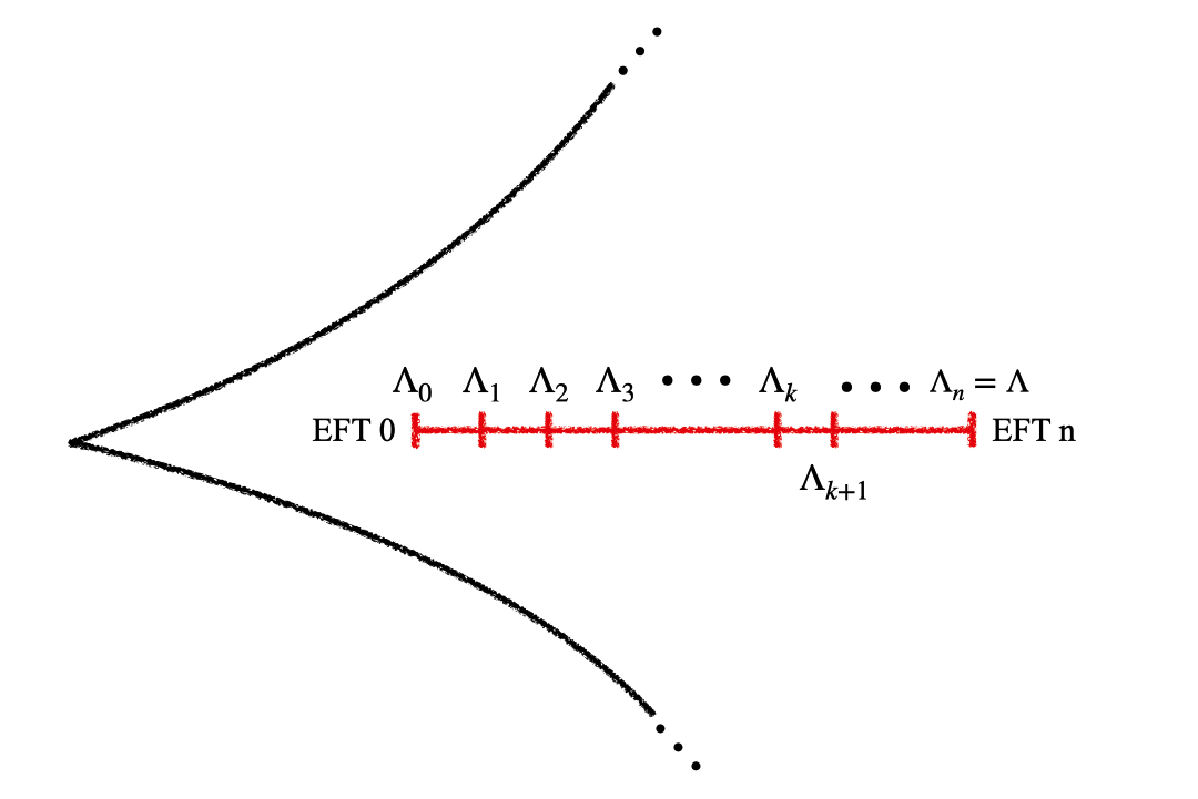
Figure 1: We can divide the path in the moduli space from $\Lambda_{0}$ to $\Lambda\gg\Lambda$ to many intervals each satisfy condition (56)

Given that $\mu_{\text{conf}}(\Lambda_{i})\gtrsim\sqrt{\Lambda_{i}}$ holds, then for the $i$th interval

$$\mu_{\text{conf}}(\Lambda_{i+1})\gtrsim\sqrt{\Lambda_{i+1}},$$ (62)

holds if

$$-\frac{k_{i}r_{i}}{\beta_{0,i}g_{0,i}^{2}}\gtrsim\frac{1}{16\pi^{2}}.$$ (63)

Thus, if the FL bound is satisfied at point $\Lambda_{0}$ then through the generalized distance conjecture it is satisfied at every other point in the moduli space $\mu_{\text{conf}}(\Lambda_{i})\gtrsim\sqrt{\Lambda_{i}}$, $i=1,\dots,n$.

3.2 Dark Dimension Scenario

Recently, it is argued that the present universe with $\Lambda\sim 10^{-122}$ is an asymptotic limit in the field space. According to the (A)dS distance conjecture a tower of light states with mass scale $m\sim\Lambda^{\alpha}$ emerges in this limit where $\nicefrac{{1}}{{4}}\leq\alpha\leq\nicefrac{{1}}{{2}}$. The experimental and theoretical bounds imply that in the current universe $\alpha=\frac{1}{4}$, and the tower is associated with decompactification of exactly one large extra dimension of radius

$$R\sim m^{-1}\sim\Lambda^{-\alpha},$$ (64)

called dark dimension (see [28, 29, 30, 31, 32, 33, 34] for related works and implications).

The canonical field that measures the distance between dS vacua with different radii of the dark dimension is given by (55) so if the radius of the dark dimension changes from $R_{0}$ to $R$ then the distance is

$$\Phi=-\frac{k}{\alpha}\ln\frac{R}{R_{0}}.$$ (65)

We note that $\Phi\sim\ln{\cal V}\sim\ln R$ which is in agreement with the examples we considered from string theory. As long as $|\text{log}(\nicefrac{{R}}{{R_{0}}})|\lesssim 1$ we have $|\Phi|<1$ and the expansion (8) can be trusted. Then, to leading order the gauge kinetic function is

$$f(\Phi) \simeq \frac{1}{g_{0}^{2}}\Big{(}1-\frac{kr}{\alpha}\ln\frac{R}{R_{0}}\Big{)}.$$ (66)

Apparently, the gauge coupling changes with the radius of dark dimension and thus confinement scale is read as

$$\mu_{\text{conf}}(R) = \mu_{\text{conf}}(R_{0})\left(\frac{R}{R_{0}}\right)^{\frac{8\pi^{2}kr}{\alpha g_{0}^{2}\beta_{0}}}.$$ (67)

The confinement scale has power law dependence on the radius of dark dimension.

To be more specific about behaviour of the confinement scale as radius of the dark dimension changes, we must determines sign of the order one parameter $r$. For the sake of concreteness, we consider the Standard Model gauge fields localised on a GUT $D_{7}$ brane in the context of F-theory [35]. Two length scales can be defined as

$$R_{S} \equiv {\cal V}(S)^{\nicefrac{{1}}{{4}}},$$ (68)

$$R_{B} \equiv {\cal V}(B)^{\nicefrac{{1}}{{6}}},$$ (69)

where $B$ is the base of the $CY_{4}$ and $S$ is the localization brane of the SM. The radius of dark dimension, the radius normal to $S$, is

$$R=R_{B}\Big{(}\frac{R_{B}}{R_{S}}\Big{)}^{\nu},$$ (70)

where for tubular geometries which describe dark dimension scenario $\nu\sim 2$. After compactification to four dimensions we find the gauge kinetic function as

$$f\simeq\frac{R_{S}^{4}}{R_{B}^{3}}.$$ (71)

Then, we find

$$\frac{\partial f}{\partial R}=\frac{\partial f}{\partial R_{B}}\left(\frac{\partial R}{\partial R_{B}}\right)^{-1}+\frac{\partial f}{\partial R_{S}}\left(\frac{\partial R}{\partial R_{S}}\right)^{-1}=-\frac{(4+7\nu)}{\nu(1+\nu)}\left(\frac{R_{S}}{R_{B}}\right)^{4+\nu}<0,$$ (72)

and consequently

$$r<0.$$ (73)

This is a generic property that the gauge kinetic function of a localised gauge theory increases when radius of dark dimension decreases. The gauge kinetic function of the gauge theory is proportional to its localization volume; the radius of the dark dimension increases as the ratio of the total radius to localization radius increases.

Finally, we find the condition that the FL bound is satisfied by a localized Yang-Mills theory in the dark dimension scenario. Assume that along a path in the moduli space the dark dimension radius changes from $R_{0}$ to $R$ such that $R_{0}>R$ or equivalently $\Lambda_{0}<\Lambda$. We recall that positive distance between the two points in the space of metrics implies $k>0$. Then given that $r$ and $k$ are negative and positive order one constants respectively, (61) implies that the following condition must be satisfied so that the FL bound holds in the vacuum with higher cosmological constant

$$0<\beta_{0}\lesssim\frac{16\pi^{2}}{g_{0}^{2}},$$ (74)

where $g_{0}$ is the tree level gauge coupling at string scale. It runs with energy due to loop corrections and matches to the experimental values measured at low energy. In Figure 2 we plot (74) for $g_{0}$ versus $\beta_{0}$ where the blue region is the parameter space of Yang-Mills theories that respect the FL bound. In this figure, We note that for a given gauge coupling at the string scale the beta function coefficient, which is fixed by the field content of the gauge theory, is bounded. For instance, if the beta function is dominated by the self interaction of gluons (which is the case for confining theories) then $\beta_{0}\simeq\nicefrac{{11}}{{3}}N_{c}$ and we find that the rank of the gauge group is bounded

$$N_{c}\lesssim 10^{3}.$$ (75)

The black dot shows the Standard Model QCD with $\beta_{0}=9$ and $g_{0}^{\text{QCD}}=0.7$ at the unification scale which is confining today and is so in any other dS vacuum with higher cosmological constant.

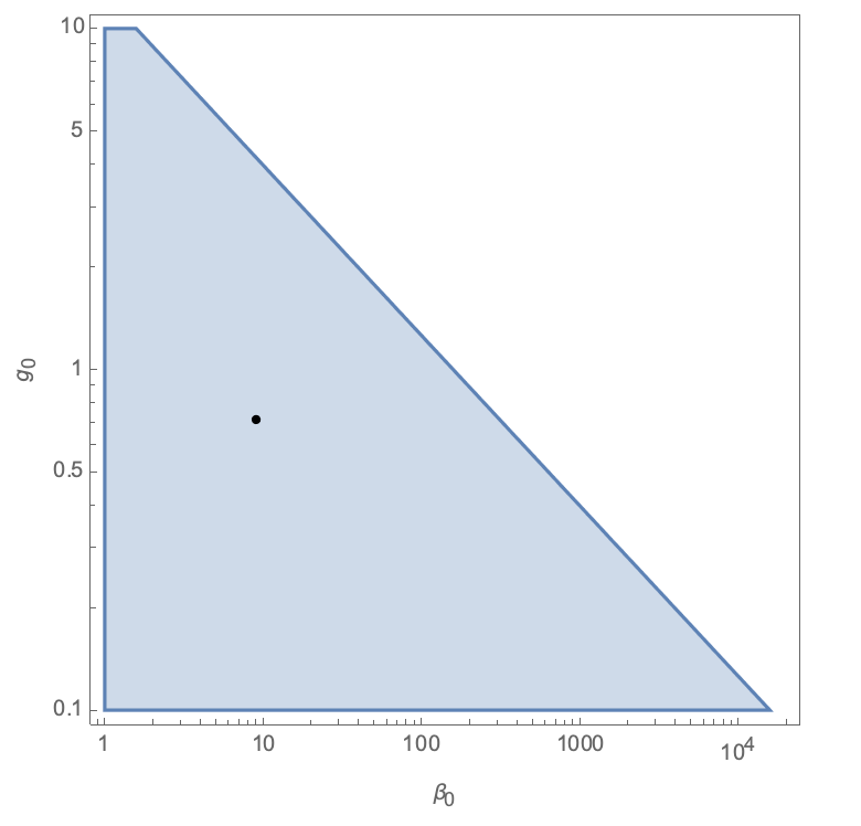
Figure 2: The gauge coupling versus the beta function coefficient. The blue region is the parameter space of Yang-Mills theories with satisfy (74). The black dot is the Standard Model QCD.

4 Conclusion

In this paper we studied dependence of gauge coupling on distance in the space of metric configurations in a theory of quantum gravity. We considered supersymmetric compactifications of heterotic, type IIA with $D6$ branes, type IIB with $D7/D3$ branes, type IIB with $D9/D5$ branes and argued that gauge coupling and confinement scale typically depend on distance in the metric space. In the (A)dS space, our results imply that confinement scale depends on the cosmological constant. We found the condition that the swampland FL bound for confinement scale of a gauge theory in dS space be realised in this framework; if the bound holds in a dS vacuum it also holds in a vacuum with higher cosmological constant, provided that stringy effects are stronger than radiative effects. Furthermore, we studied distance dependent confinement scale for gauge fields localised on a brane in dark dimension scenario. We argued that confinement scale increases as the radius of the dark dimension decreases. We also found that the FL bound is inherited to vacua with higher cosmological constants for Yang-Mills theories with $N_{c}\lesssim 10^{3}$.

In this work, we did not compute the exact distance dependence of the gauge kinetic function; we computed the leading order terms in the expansion in small changes of distance. The next step would be to go beyond this approximation, and find out how it might be related to other swampland conjectures such as the WGC. We postpone this to a future work. Finally, for the sake of concreteness and computational ability, we have considered supersymmetric compactifications. It would be interesting to look into realistic non-supersymmetric examples. However, one expects that gauge kinetic functions depend on volume moduli and the dilaton in every compactification which consequently induces distance dependence. It will be studied in more detail in a future work.

Acknowledgements

We would like to thank Irene Valenzuela, and Alek Bedroya for useful comments and illuminating discussions. AM is thankful to TH department of CERN for hospitality during the final stages of this work. MT thanks Perimeter Institute for warm hospitality.

References

- [1] C. Vafa, “The String Landscape and the Swampland,” [arXiv:hep-th/0509212 [hep-th]].
- [2] H. Ooguri and C. Vafa, “On the Geometry of the String Landscape and the Swampland,” Nucl. Phys. B 766 (2007), 21-33 doi:10.1016/j.nuclphysb.2006.10.033 [arXiv:hep-th/0605264 [hep-th]].
- [3] T. D. Brennan, F. Carta and C. Vafa, “The String Landscape, the Swampland, and the Missing Corner,” PoS TASI2017 (2017), 015 doi:10.22323/1.305.0015 [arXiv:1711.00864 [hep-th]].
- [4] E. Palti, “The Swampland: Introduction and Review,” Fortsch. Phys. 67 (2019) no.6, 1900037 doi:10.1002/prop.201900037 [arXiv:1903.06239 [hep-th]].
- [5] M. van Beest, J. Calderón-Infante, D. Mirfendereski and I. Valenzuela, “Lectures on the Swampland Program in String Compactifications,” [arXiv:2102.01111 [hep-th]].
- [6] Agmon, N., Bedroya, A., Kang, M. and Vafa, C. Lectures on the string landscape and the Swampland. (2022,12)
- [7] Gonzalo, E., Ibáñez, L. and Valenzuela, I. Swampland constraints on neutrino masses. JHEP. 2 pp. 088 (2022)
- [8] Ibanez, L., Martin-Lozano, V. and Valenzuela, I. Constraining Neutrino Masses, the Cosmological Constant and BSM Physics from the Weak Gravity Conjecture. JHEP. 11 pp. 066 (2017)
- [9] Ibanez, L., Martin-Lozano, V. and Valenzuela, I. Constraining the EW Hierarchy from the Weak Gravity Conjecture. (2017,7)
- [10] Montero, M., Vafa, C. and Valenzuela, I. The Dark Dimension and the Swampland. ArXiv Preprint ArXiv:2205.12293. (2022)
- [11] Banks, T. & Seiberg, N. Symmetries and strings in field theory and gravity. Physical Review D. 83, 084019 (2011)
- [12] Ooguri, H. & Vafa, C. On the Geometry of the String Landscape and the Swampland. Nuclear Physics B. 766, 21-33 (2007)
- [13] Arkani-Hamed, N., Motl, L., Nicolis, A. & Vafa, C. The string landscape, black holes and gravity as the weakest force. Journal Of High Energy Physics. 2007, 060 (2007)
- [14] Obied, G., Ooguri, H., Spodyneiko, L. & Vafa, C. de Sitter Space and the Swampland. ArXiv Preprint ArXiv:1806.08362. (2018)
- [15] Ooguri, H., Palti, E., Shiu, G. & Vafa, C. Distance and de Sitter Conjectures on the Swampland. Physics Letters B. 788 pp. 180-184 (2019)
- [16] Bedroya, A. & Vafa, C. Trans-Planckian censorship and the swampland. Journal Of High Energy Physics. 2020, 1-34 (2020)
- [17] M. Montero, C. Vafa, T. Van Riet and G. Venken, “The Fl Bound and Its Phenomenological Implications,” JHEP 10 (2021), 009 doi:10.1007/JHEP10(2021)009 [arXiv:2106.07650 [hep-th]].
- [18] M. Montero, T. Van Riet and G. Venken, “Festina Lente: Eft Constraints from Charged Black Hole Evaporation in De Sitter,” JHEP 01 (2020), 039 doi:10.1007/JHEP01(2020)039 [arXiv:1910.01648 [hep-th]].
- [19] Lüst, D., Palti, E. and Vafa, C. AdS and the Swampland. Physics Letters B. 797 pp. 134867 (2019)
- [20] Polchinski, J. String theory. (2005)
- [21] Ibanez, L. and Uranga, A. String theory and particle physics: An introduction to string phenomenology. (Cambridge University Press,2012)
- [22] Mishra, R. Confinement in de Sitter Space and the Swampland. Journal Of High Energy Physics. 2023, 1-22 (2023)
- [23] K. Ban, D. Y. Cheong, H. Okada, H. Otsuka, J. C. Park and S. C. Park, “Phenomenological Implications on a Hidden Sector from the Festina Lente Bound,” [arXiv:2206.00890 [hep-ph]].
- [24] S. M. Lee, D. Y. Cheong, S. C. Hyun, S. C. Park and M. S. Seo, “Festina-Lente Bound on Higgs Vacuum Structure and Inflation,” JHEP 02 (2022), 100 doi:10.1007/JHEP02(2022)100 [arXiv:2111.04010 [hep-ph]].
- [25] Mohseni, A. and Torabian, M. Higgs in Nilpotent Supergravity: Vacuum Energy and Festina Lente. (2022,7)
- [26] V. Guidetti, N. Righi, G. Venken and A. Westphal, “Axionic Festina Lente,” [arXiv:2206.03494 [hep-th]].
- [27] M. Montero, J. B. Muñoz and G. Obied, “Swampland Bounds on Dark Sectors,” [arXiv:2207.09448 [hep-ph]].
- [28] Gonzalo, E., Montero, M., Obied, G. and Vafa, C. Dark Dimension Gravitons as Dark Matter. (2022,9)
- [29] Anchordoqui, L., Antoniadis, I., Cribiori, N., Lust, D. and Scalisi, M. The Scale of Supersymmetry Breaking and the Dark Dimension. (2023,1)
- [30] Anchordoqui, L., Antoniadis, I. and Lust, D. Aspects of the Dark Dimension in Cosmology. (2022,12)
- [31] Anchordoqui, L., Antoniadis, I. and Lust, D. The dark universe: Primordial black hole dark graviton gas connection. Phys. Lett. B. 840 pp. 137844 (2023)
- [32] Blumenhagen, R., Brinkmann, M. and Makridou, A. The dark dimension in a warped throat. Phys. Lett. B. 838 pp. 137699 (2023)
- [33] Anchordoqui, L., Antoniadis, I. and Lust, D. Dark dimension, the swampland, and the dark matter fraction composed of primordial black holes. Phys. Rev. D. 106, 086001 (2022)
- [34] Anchordoqui, L. Dark dimension, the swampland, and the origin of cosmic rays beyond the Greisen-Zatsepin-Kuzmin barrier. Phys. Rev. D. 106, 116022 (2022)
- [35] Beasley, C., Heckman, J. & Vafa, C. GUTs and exceptional branes in F-theory—II. Experimental predictions. Journal Of High Energy Physics. 2009, 059 (2009)