Randomization Inference When N Equals One

Abstract

N-of-1 experiments, where a unit serves as its own control and treatment in different time windows, have been used in certain medical contexts for decades. However, due to effects that accumulate over long time windows and interventions that have complex evolution, a lack of robust inference tools has limited the widespread applicability of such N-of-1 designs. This work combines techniques from experiment design in causal inference and system identification from control theory to provide such an inference framework. We derive a model of the dynamic interference effect that arises in linear time-invariant dynamical systems. We show that a family of causal estimands analogous to those studied in potential outcomes are estimable via a standard estimator derived from the method of moments. We derive formulae for higher moments of this estimator and describe conditions under which N-of-1 designs may provide faster ways to estimate the effects of interventions in dynamical systems. We also provide conditions under which our estimator is asymptotically normal and derive valid confidence intervals for this setting.

Keywords— causal inference, system identification, potential outcomes, interference, time series.

1 Introduction

Randomized experiments are arguably the most important contribution of twentieth-century statistics, providing a program to establish the value of interventions to populations of individuals. By randomly assigning individuals to treatment and control, statistical analysis can simultaneously determine the magnitude of intervention effects and eliminate confounding explanations. However, a significant drawback of randomized experiments is that they yield conclusions about populations rather than individuals. When treatments present heterogeneous effects, a randomized experiment cannot inform individuals whether a treatment can work for them.

Is it possible to design experiments for individuals? N-of-1 trials attempt to solve this problem by having individuals apply randomized treatments in different time windows. The individual becomes the treatment and the control. N-of-1 trials are within-patient randomized controlled trials, where the treatment is randomized at every time period, with the subject potentially crossing over between treatment and control at each phase.

In medicine, the formalized N-of-1 trial is nearly as old as the randomized clinical trial itself. In 1950, only a few years after the famous randomized trials of Streptomycin, Quin and colleagues performed randomized within subject trials of an arthritis reduction agent where patients received a random treatment at multiple doctor visits [19]. D. D. Reid explained Latin Square designs for N-of-1 trials and explored these for testing the effectiveness of laxatives [21] and arthritis ointments [20]. Snell and Armitage tested heroin as a cough suppressant with N-of-1 designs [26]. Bradford Hill even devotes a lengthy part of the Clinical Trials chapter (pages 260-263) in his Principles of Medical Statistics to the design of N-of-1 trials [10].

Since the 1950s, though never a dominant experimental design, N-of-1 trials have continued to find application. Louis et al. reported 28 self-controlled studies in the New England Journal of Medicine in 1978 and 1979 [13]. Guyatt et al. argued for using N-of-1 trials as part of general clinical practice with patients, helping individuals find the best treatment for them [8]. N-of-1 trials have been recently used successfully to test the side effects of statin treatments [30].

In the online experimentation community, N-of-1 experiments are often called switchback or interleaving designs. Netflix and LinkedIn use N-of-1 designs to test the time-varying effects of their recommendation and matching algorithms. For example, [3] reports interleaving online experiments where a client is randomly exposed to different app experiences for 30-minute intervals. N-of-1 designs have the potential to be tailored to personalized experiments to improve the experience of individual customers. Moreover, N-of-1 designs enable data scientists to mitigate interference effects from multiple AB tests running concurrently [27].

If the effect is immediate and transient, standard tools from randomized experiments can be used to estimate its magnitude and significance in N-of-1 trials. However, when the effect of an intervention persists over time, it becomes challenging to draw proper inferences. Though recent estimators have attempted otherwise, most N-of-1 designs try to reduce the problem to a randomized experiment where each time period is independent. In such a case, the treatment must take effect and cease rapidly. These designs also must assume an individual’s baseline is roughly constant. For these reasons, N-of-1 designs have primarily focused on chronic conditions treatable by acute medications.

Can we do better? In this work, we aim to combine techniques from experiment design in causal inference with system identification from control theory to provide a general inference framework for N-of-1 experiments. In what follows, we describe the foundational pillars of our framework and a view of how they might be combined for inferring effects in N-of-1 experiments. We then present a formal interference model for temporal effects drawn from the literature on dynamical systems. We define a family of estimands of causal effects of these models and then present a reasonable, unbiased estimator for this family. We demonstrate that this estimator is asymptotically normal and provide a plug-in estimator for its variance. Together, these enable the construction of valid confidence intervals. Along the way, we discuss the inferential challenges of this framework and why our approach, though more general than previous methods, remains limited.

1.1 Foundational Related Work

Our work draws and expands upon the literature on causal inference and system identification. In this section, we elaborate on the background and how we will attempt to reconcile these two different lines of research.

Causal inference

The potential outcomes framework [15, 22] offers a systematic and rigorous approach to studying causal relationships in experimental and observational studies. In the simplest setting, a unit $i$ has two potential outcomes under an intervention (also called a treatment). The observed outcome of unit $i$ is denoted by $y_{i}$, and we distinguish the outcome under no treatment as $y_{i}(0)$ and under treatment as $y_{i}(1)$. If we let $x_{i}$ denote the binary indicator equal to $1$ when treatment is applied and $0$ when treatment is not applied, then we have the expression

$$y_{i}:=y_{i}(1)\cdot x_{i}+y_{i}(0)\cdot(1-x_{i})$$

This formula holds regardless of whether $y_{i}$ are real-valued or binary outcomes.

Though this formula looks like it is tautological, it makes some hidden assumptions. In particular, this model assumes that the treatment applied to unit $i$ only impacts unit $i$. This is called the Stable Unit Treatment Values Assumption (SUTVA). This assumption does not hold for within-unit trials. If a treatment is applied in succession to a unit, care must be taken to ensure that the previous treatment does not influence the outcomes of future treatments.

When the $x_{i}$ can be intentionally assigned, random assignment enables estimation of the average outcome under treatment and control. That is, if we are interested in estimating the quantity

$$\tau:=\tfrac{1}{n}\sum_{i=1}^{n}y_{i}(1)-y_{i}(0)\;,$$

we can do an experiment where $x_{i}$ is assigned at random and then estimate $\tau$ from the observed outcomes.

Assume, for simplicity, that the $x_{i}$ are assigned as independent Bernoulli coin flips. Denote the centered treatment variable $z_{i}=2x_{i}-1\in\{\pm 1\}$. Then the Horvitz-Thompson estimator $\widehat{\tau}_{\mathrm{HT}}$

$$\widehat{\tau}_{\mathrm{HT}}:=\tfrac{2}{n}\sum_{i=1}^{n}z_{i}\cdot y_{i}\;$$

is an unbiased estimator of the average treatment effect. When SUTVA applies, inference about the significance of causal effects is also elegant. $\widehat{\tau}_{\mathrm{HT}}$ is asymptotically normal, and confidence intervals can be constructed using upper bounds on the variance of $\widehat{\tau}_{\mathrm{HT}}$ (see, for example, [11]).

Beyond SUTVA

For causal questions about time series data, SUTVA rarely applies [25, 7]. Suppose now that each unit is indexed by time. Suppose we have a sequence of interventions at each time $x_{1}$, $x_{2},\ldots,x_{T}$. Even if these interventions are binary-valued, the outcome at time $t$, $y_{t}$ could potentially depend on all of the outcomes that have occurred before time $t$. Namely, $y_{t}$ is potentially a function of $x_{1},\ldots,x_{t}$. We could represent $y_{t}$ then as a sum over all possible interactions. That is,

$$y_{t}=\sum_{S:S\subseteq\{0,1,\ldots,t\}}\alpha_{t,S}\cdot\prod_{i\in S}z_{i}\;,$$ (1.1)

where again, $z_{i}=2x_{i}-1$. The standard Potential Outcomes framework is the special case when the coefficients $\alpha_{t,S}=0$ for all $S\neq\emptyset$ or $\{t\}$. This basis expansion is fully general as it is the Fourier expansion of $y_{t}(x_{0},x_{1},\ldots,x_{t})$ [16]. But the expansion has a number of terms that grows exponentially with $t$, preventing any meaningful statistical analysis.

Since a full representation is intractable, more restricted interactions have been studied. The Granger-Sims causality framework [7, 25, 1] tests correlations in $x$’s that can explain $y$. For example, in its simplest form, Granger Sims studies how well linear expansions of the form

$$y_{t}=\alpha_{\emptyset}+\alpha_{0}\cdot x_{t}+\alpha_{1}\cdot x_{t-1}+\ldots+\alpha_{t}\cdot x_{0}+\mathrm{error}_{t}$$

predict outcomes. Granger causality assumes time-invariance to provide practically useful answers to understand when time series can predict each other.

In this paper, we study this time-invariant model, under the assumption that the $x_{i}$ are chosen interventionally as part of an experiment.

System identification

In control theory, modeling the input-output behavior of a dynamical system is a first step in designing a feedback policy. Such dynamical systems are assumed to obey dynamical equations of the form

$$s_{t+1}=f_{t}(s_{t},x_{t},\varepsilon_{t}),~{}~{}y_{t}=h_{t}(s_{t},x_{t},\varepsilon_{t})\,.$$

$x_{t}$ in this context is a controllable input to the dynamical system. $y_{t}$ is the measured output and $\varepsilon_{t}$ is an exogenous noise process. $s_{t}$ is the state of the dynamical system. The state is the variable that makes future outputs conditionally independent of past outputs.

The goal in system identification is to find appropriate estimates of the function $f_{t}$ and $h_{t}$ so that inputs $x_{t}$ can be planned to steer $y_{t}$ to desired values.

Just as we have described above, the identification problem is only tractable if the class of models for $f_{t}$ and $h_{t}$ is simple enough. Several reduced model classes are useful for representing dynamical systems. One of the most fundamental models assumes that the functions $f_{t}$ and $h_{t}$ are linear (but might vary over time). In such a case, we can write the input-output map as

$$y_{t}=\sum_{k\leq t}G_{tk}x_{k}+e_{t}$$

where $G_{tk}$ are scalars and $e_{t}$ are linear functions of the $\varepsilon_{k}$ variables and $s_{1}$.

Under a further restriction, we can assume the system is linear and time-invariant so that $f_{t}=f$ and $h_{t}=h$ for all $t$. In this case, $y_{t}$ can be written as a linear convolution of $x_{k}$ and a sequence $g_{k}$:

$$y_{t}=\sum_{k\leq t}g_{t-k}x_{k}+e_{t}\,.$$

This model is the same as the 1-step Granger Causality model described in the previous section.

Identifying linear time-invariant systems has a rich literature (see the textbook by Ljung [12]). Importantly, the choice of $x_{k}$ matters as this input design must make all $g_{k}$ of interest identifiable. The most popular choice in theory and practice chooses $x_{k}$ to be an i.i.d. sequence of zero mean random variables. In practice, it suffices that these variables take on two values, such as $1$ and $-1$ [14, 29, 17]. When restricted to such signed inputs, the linear system identification problem looks like a Potential Outcomes estimation problem under a linear interference model.

Though there is extensive literature on system identification, only recently have researchers determined statistical error rates for the estimation of the sequence $g_{k}$ from a single input sequence $x_{k}$. There are numerous reasons for this. First, since system identification of engineered systems is typically done in a controlled setting, sample complexity is not typically a constraint on engineers. Second, the statistical methods for system identification lean on random matrix results that have only been recently derived.

The analysis of Oymak and Ozay [18] shows that the parameters $g_{k}$ can be estimated via least squares when $x_{t}$ and $e_{t}$ are zero-mean Gaussian random variables and $s_{1}=0$. They further assume that $g_{k}$ obeys a decay condition that $|g_{k}|\leq Ca^{k}$ for a constant $C$ and $a<1$. They show that the rate of error in the estimate $\hat{g}_{k}$ satisfies

$$\sum_{k=1}^{\infty}|g_{k}-\hat{g}_{k}|^{2}=O\left(\tfrac{1}{(1-a)^{2}T}\right)$$

where $T$ is the number of observed samples.

Later work by Simchowitz et al. [24] removed the dependence on $a$ in exchange for another property of $g$ called phase rank, but some restriction on the form of $g$ is always required to estimate $g$. Similarly, work by Bakshi et al. [2] provides tighter bounds on this estimation error, but assumes the error signal is random and the input signal is zero mean. Moreover, the current system identification literature does not provide provable means of data-driven uncertainty quantification, a crucial component of causal inference.

A synthesis of causal inference and system identification

The work in this paper builds on these three pillars to synthesize an inference framework for N-of-1 experiments. First, as we develop in the next section, we focus on the linear time-invariant outcome model studied in Granger-Sims causality, and in linear system identification

$$y_{t}=\sum_{s=0}^{t}x_{s}g_{t-s}+e_{t}\,.$$ (1.2)

This model generalizes the Neyman-Rubin framework to allow for a particular functional form of linear interference that is inspired by linear dynamical systems. In the next section, we develop a generalization of the Horvitz-Thompson estimator for linear estimands of the form

$$\tau(q):=\langle g,q\rangle\,.$$

In the case that $q$ is the first standard basis vector, the generalized estimator will precisely be the Horvitz-Thompson estimator.

Unlike in the Granger-Sims and linear system identification frameworks, we do not assume the error signal $e_{t}$ is random in (1.2). We will focus on estimating various linear functionals of the coefficients $g\in\mathbb{R}^{T}$. Focusing on linear estimands rather than the coefficients themselves should simplify the problem. We note, however, that results for this simplification cannot be derived from the prior art.

Additionally, in this work, we are interested in estimating $g_{k}$ when $e_{t}$ is a non-random signal. Simchowitz et al. [24] were the first to study estimation of $g$ when $e_{t}$ was non-random, and estimation under non-random conditions has been used in the study of online control [9]. However, none of these works provided specific forms of the error, nor did they quantify the variance sufficiently accurately for the construction of asymptotically-sharp confidence intervals.

However, the explicit form of the error is not provided. There are several practically relevant situations where such non-random noise arises. For instance, suppose we restrict our attention to input sequences that are constrained to be nonnegative. This departs from the zero-mean inputs in Granger-Sims and system identification. Non-zero-mean inputs can be modeled as zero-mean inputs plus a new, non-random error term.

Unlike system identification, our work is interested in estimating confidence intervals on linear functionals of $g_{k}$ from finite experiments. None of the prior work has investigated such uncertainty quantification. In particular, we derive novel asymptotic normality guarantees for our estimator, which is closely related to the least-squares estimator of Oymak and Ozay [18] and the method-of-moments estimator of Bakshi et al. [2]. The proof of asymptotic normality is more delicate than what is typical of Horvitz-Thompson estimators. In particular, the asymptotic normality requires an intricate calculation balancing of eighth moments of the intervention variables.

Finally, we close this discussion with a discussion of recent complementary work in the context of online experiments. Bojinov et al. explored experiments on time series using the potential outcome framework for switchback experiments [4]. There, the authors consider a general time-varying outcome model with only short-term dependence on the experiment variable. Their experimental estimand focuses on average short-term effects, whereas our estimand considers any linear functional of the long-term response. The salient distinction from the present work is the focus on general, short-term effects versus linear, long-term effects. In this way, our papers complement each other and point to the potential of a general framework that can effectively handle general, long-term interference effects in N-of-1 trials.

2 Convolutions

The outcomes in linear time-invariant models can be represented as a convolution between an intervention sequence and a parameter vector known as an impulse response. Before expanding on our statistical theory, we first review the basic notation and theory of convolution. This notation will simplify many of the formulas, and eliminate the need to track subscripts.

Let $u_{t}$ and $v_{t}$ be two signals with indices in the nonnegative integers. The convolution of $u_{t}$ and $v_{t}$ is the signal

$$(u*v)_{t}=\sum_{s=0}^{t}u_{s}v_{t-s}$$

Note how this expression allows us to compactly rewrite the models of Granger-Sims causality and LTI systems.

Convolution is commutative ($u*v=v*u$) and linear. We can write the operator that takes $v$ to $u*v$ in matrix form

$$u*v=\mathcal{T}_{u}v$$

where $\mathcal{T}_{u}$ is the Toeplitz matrix

$$\mathcal{T}_{u}=\begin{bmatrix}u_{0}&0&0&0&\ldots&0\\ u_{1}&u_{0}&0&0&\ldots&0\\ u_{2}&u_{1}&u_{0}&0&\ldots&0\\ \vdots&\vdots&\vdots&\ddots&\vdots&\vdots\\ u_{T-1}&u_{T-2}&u_{T-3}&\ldots&\ldots&u_{0}\end{bmatrix}\,.$$

Note that we must have $\mathcal{T}_{u}v=\mathcal{T}_{v}u$.

The adjoint operator of $\mathcal{T}$ maps matrices to vectors with components

$$\mathcal{T}^{*}(M)_{s}=\sum_{t}M_{t,t-s}\;.$$

Moreover, we have the composition $\mathcal{T}^{*}(\mathcal{T}_{u})_{s}=(T-s+1)u_{s}$.

In our theoretical analysis, we use circular extensions of signals that result in tractable closed-form expressions for many of the moments in our experiment designs. For two signals $u$ and $v$ of length $T$, the circular convolution is defined as

$$(u\oast v)_{t}=\sum_{s=0}^{T-1}u_{s}v_{t-s\pmod{T}}\;,$$

where the circular extention notation $\pmod{T}$ means that for $s\in[0,t],t-s\pmod{T}=t-s$ and for $s\in(t,T-1],t-s\pmod{T}=T+t-s$. Note here that the summation extends over all possible indices $s$, not just those that have values less than or equal to $t$. In matrix form, circular convolution corresponds to multiplication by a circulant matrix

$$u\oast v=\mathcal{C}_{u}v$$

where $\mathcal{C}_{u}$ is the matrix

$$\mathcal{C}_{u}=\begin{bmatrix}u_{0}&u_{T-1}&u_{T-2}&u_{T-3}&\ldots&u_{1}\\ u_{1}&u_{0}&u_{T-1}&u_{T-2}&\ldots&u_{2}\\ u_{2}&u_{1}&u_{0}&u_{T-1}&\ldots&u_{3}\\ \vdots&\vdots&\vdots&\ddots&\vdots&\vdots\\ u_{T-1}&u_{T-2}&u_{T-3}&\ldots&\ldots&u_{0}\end{bmatrix}\,.$$

For a variety of reasons, computation with circular convolutions is more elegant than with linear convolutions. For example, the Discrete Fourier Transform of a circular convolution is the product of the Discrete Fourier Transforms of the individual signals. Such properties will be used in depth in the theoretical analysis.

For the ease of writing subscripts in equations, we introduce the circular extension notation $v^{\circ}_{t}=v_{t\pmod{T}}$ for possible negative integer $t$. With this notation,

$$(u\oast v)_{t} =\sum_{s=0}^{T-1}u_{s}v^{\circ}_{t-s}\;.$$ (2.1)

3 Estimands and Estimators of Time-invariant Treatment Effects

Suppose we have a scalar outcome sequence $y_{t}$ that depends on a scalar treatment $x_{t}$ via a linear dynamical system

$$y_{t}=\sum_{s=0}^{t}g_{s}x_{t-s}+e_{t}=(g*x)_{t}+e_{t}\,.$$ (3.1)

Here $g$ is the impulse response of the linear system. For simplicity, we assume that the $x_{t}$ are binary-valued, but we expect extensions to real-valued inputs to be relatively straightforward.

$e_{t}$ is an exogenous signal that is not affected by the treatment $e_{t}$. But we are interested in analyzing $e_{t}$ that are far from random. As a motivating example, suppose two treatments have treatment effects $g_{0}$ and $g_{1}$. We are interested in which leads to overall better outcomes. In this case, $g=g_{1}-g_{0}$ and $e=g_{0}$. These signals are tightly correlated. Hence, we model $e$ as an adversarial error oblivious to the randomization $x$. The error could be non-i.i.d., non-stationary, and even systematic, as long as it is oblivious to input $x$.

Which outcome properties might we be interested in? We could study the average treatment effect, which compares outcomes when $x_{t}$ is equal to either all ones or all zeros:

$$\tau_{\mathrm{ATE}}=\tfrac{1}{T}\sum_{t=1}^{T}y_{t}(1)-y_{t}(0)$$

Using (3.1), we can write $\tau_{\mathrm{ATE}}$ in terms of the impulse response

$$\tau_{\mathrm{ATE}}=\sum_{t=1}^{T}\tfrac{(T-t+1)}{T}g_{t}\,.$$

Hence, for full generality, we will study linear estimands of the form $\tau(q)=\langle D_{T}q,g\rangle$ where $q$ is a vector and $D_{T}$ is the diagonal matrix with $t$-th entry $\frac{T-t+1}{T}$. With this definition, $\tau_{\mathrm{ATE}}=\tau(q)$ when $q=\mathbf{1}$.

For these designs, different estimands can highlight varied intervention effects. In a standard N-of-1 trial, the estimand would compare the effects of treatments at the end of each dosing period. That is, if a particular treatment is given for a week at a time, the estimand will measure outcomes at the end of each week. Standard N-of-1 designs use long periods to ensure that the interference between the effects of the different treatments have washed out before an outcome is measured. If a treatment has spillover, then measurements early in a treatment period will be influenced by the prior period’s treatment.

But what if we are interested in the average treatment effect at the resolution of a day? We can likely measure outcomes each day, but can we measure the average differences? To get a feel for how these two estimands can be different, consider the following two treatments with two periods:

$$y_{1}^{A}=x_{1}\,,~{}~{}~{}y_{2}^{A}=x_{1}+x_{2}\;,$$

and

$$y_{1}^{B}=0\,,~{}~{}~{}y_{2}^{B}=2x_{1}\,.$$

Both of these treatments correspond to linear time-invariant systems with $g^{A}=(1,1)$ and $g^{B}=(0,2)$.

For both treatments, the outcome if the treatment is taken for two time periods is $2$. However, the average outcome for Treatment A is $1.5$ and the average outcome for Treatment B is $1$. If, for example, these treatments are pain medications, then Treatment A is preferable to Treatment B as the immediate relief is valuable. We thus aim to allow for a variety of linear estimands to capture the effect most aligned with preferred outcomes.

3.1 Estimation from Random Design

Consider the randomized experiment where we assign the input at time $t$ to be zero or one with equal probability, independently at each $t\in[T]$. How can we estimate the treatment effect $\tau(q)$ from the observed outcomes of an experiment?

We now fix the notation for the remainder of the document to distinguish between random and nonrandom signals. We will use boldface font for random vectors to emphasize the stochastic nature of experimentation. In what follows, we use the normal font, say $x\in\mathbb{R}^{T}$ and $H\in\mathbb{R}^{T\times T}$ to denote deterministic vectors and matrices, and boldface say $\mathbf{x},\mathbf{y},\mathbf{z},\mathbf{W}$ to denote vectors that are random due to experimental design. The lone exception is that we use $\mathbf{1}$ to denote the all ones vector and avoid confusion with the scalar $1$.

With our fixed notation, the linear convolution model is written as

$$\mathbf{y}=\mathbf{x}*g+e\in\mathbb{R}^{T}\;,$$ (3.2)

and $g,\mathbf{x},\mathbf{x}*g$ and $e$ are all of length $T$ with $\mathbf{x}_{t}\in\{0,1\},t\in[T]$.

A natural generalization of the Horvitz-Thompson estimator is the method-of-moments estimator discussed above.

$$\widehat{\tau}(q)=\tfrac{1}{T}\langle(2\mathbf{x}-\mathbf{1})*q,2\mathbf{y}\rangle\,.$$ (3.3)

This choice is natural in the following sense. Suppose we restrict our attention to unbiased linear estimators $\langle w,\mathbf{y}\rangle$. Then unbiasedness is the linear constraint

$$\mathop{\mathbb{missing}}{E}_{\mathbf{x}}[\langle w,\mathbf{y}\rangle]=\langle D_{T}q,g\rangle\,.$$

Setting $w$ as the Moore-Penrose pseudoinverse of this system of equations yields the estimator (3.3).

As we will do several times in what follows, we note that $\widehat{\tau}(q)$ is a quadratic function of $T$ independent Rademacher random variables. Throughout we will need to compute moments of such Rademacher chaos, and we provide explicit formulas for their first, second, and fourth moments in Appendix A.1.

Indeed, $\mathbf{z}=2\mathbf{x}-\mathbf{1}$ is a vector of independent Rademacher random variables and we have that

$$\widehat{\tau}(q) =\tfrac{1}{T}\langle\mathbf{z}*q,2(\mathbf{x}*g+e)\rangle=\tfrac{1}{T}\langle\mathcal{T}_{q}\mathbf{z},2\mathcal{T}_{g}\mathbf{x}+2e\rangle=\tfrac{1}{T}\left\langle\mathbf{z},\mathcal{T}_{q}^{\top}\mathcal{T}_{g}\mathbf{z}\right\rangle+\tfrac{1}{T}\left\langle\mathbf{z},\mathcal{T}_{q}^{\top}\mathcal{T}_{g}\mathbf{1}+2\mathcal{T}_{q}^{\top}e\right\rangle\;.$$

From this calculation we can verify that $\widehat{\tau}(q)$ is indeed unbiased as

$$\mathop{\mathbb{missing}}{E}[\widehat{\tau}(q)]=\tfrac{1}{T}\tr\left(\mathcal{T}_{q}^{\top}\mathcal{T}_{g}\right)=\sum_{t=1}^{T}\tfrac{T-t+1}{T}q_{t}g_{t}=\langle D_{T}q,g\rangle\;.$$

Moreover, the variance of $\hat{\tau}_{q}$ is given by

$$T^{2}\operatorname{var}(\widehat{\tau}(q))=\|\mathcal{T}_{q}^{\top}\mathcal{T}_{g}\|_{F}^{2}+\tr(\mathcal{T}_{q}^{\top}\mathcal{T}_{g}\mathcal{T}_{q}^{\top}\mathcal{T}_{g})-2\sum_{t=1}^{T}\langle\mathcal{T}_{q}u_{t},\mathcal{T}_{g}u_{t}\rangle^{2}+\|\mathcal{T}_{q}^{\top}(g*\mathbf{1}+2e)\|^{2}\;.$$ (3.4)

Here $u_{t}$ denotes the $t$-th standard basis vector. Though this variance formula can be computed from the problem data, it is not wieldy or illuminating. In the later sections, we will compute an approximate variance formula that provides more insights into the dependence of the variance on $g$, $q$, and $e$.

Example utility of N-of-1 Design

The simple variance calculations thus far have already shed some light on the utility of rapid switching in N-of-1 designs. If one wants to use a standard Horvitz-Thompson style treatment effect when implementing an N-of-1 design, the period at which the treatment is switched must be carefully chosen. Suppose a patient is trying to choose between two drugs, Drug A and Drug B. In a standard N-of-1 design, the drugs would be given over windows so that their effects wash out over time. That is, the half-life of the drug would determine the switching time.

In our N-of-1 design, the drugs can be interleaved more rapidly. The benefit of such an approach is that if there are decaying effects, the patient would experience the average response of the two treatments. But this averaging could come at the cost of having to run a longer experiment. Here, we show a toy example illustrating how the expected time required to distinguish two treatments is approximately the same.

Suppose that Drug A has an impulse response

$$g_{t}^{(1)}=Ag^{(0)}_{t}$$

and Drug B has an impulse response

$$g_{t}^{(2)}=Bg^{(0)}_{t}$$

Suppose $A$ and $B$ are positive scalars and, w.l.o.g., $A\geq B$.

The associated estimand for this treatment effect is

$$\tau_{1}=g_{0}^{(1)}-g_{0}^{(2)}=(A-B)g^{(0)}_{0}$$

This corresponds to $\tau(q)$ with $q_{1}=1$ and all other entries equalling 0.

Consider the signal-to-noise ratio, equal to

$$SNR=\frac{\tau(q)}{\sqrt{\operatorname{var}(\widehat{\tau}(q))}}\,.$$

Suppose we observe an observation length $T$. Using the variance formula (3.4), we have

$$\operatorname{var}(\widehat{\tau}(q))=\frac{(A-B)^{2}}{T}v(g^{(0)})+\frac{(A+B)^{2}}{T}w(g^{(0)})$$

where

$$v(g^{(0)}) =\sum_{t=2}^{T}\tfrac{T-t+1}{T}{g^{(0)}_{t}}^{2}\;,$$

$$w(g^{(0)}) =\tfrac{1}{T}||g^{(0)}*1||_{2}^{2}\;.$$

Note that both of these quantities are bounded for all $t$ by $\|g^{(0)}\|_{2}^{2}$. A crude bound for the variance is thus

$$\operatorname{var}(\widehat{\tau}(q))\leq\frac{(A+B)^{2}}{T}\left\{\left(\frac{A-B}{A+B}\right)^{2}v(g^{(0)})+w(g^{(0)})\right\}\leq\frac{(A+B)^{2}}{T}\left(2\|g^{(0)}\|^{2}-{g^{(0)}_{0}}^{2}\right)\;.$$ (3.5)

Thus, even with rapid interleaving of treatments, the SNR tends to infinity at a rate of $\sqrt{T}$.

We can say a bit more than this. If we do a standard experiment design where we wait $\ell$ time steps for the transient dynamics to end, measure a new outcome, and potentially switch the treatment, then the signal-to-noise ratio with random treatment assignments is

$$\frac{A-B}{A+B}\sqrt{T}\ell^{-1/2}\,.$$

We can compare the signal-to-noise ratios of the rapid design to the conservative design for particular models of $g^{(0)}$. As an illustrative example, suppose that $g^{(0)}_{t}=\beta^{t}$. That is, it’s a simple exponential decay. Suppose $t$ indexes days and $\beta=0.5$. This means that the treatment has a half-life of one day. For an N-of-1 experiment that requires the effect to clear, this means you should wait 4-5 days between switching treatments. Let us choose 4 for convenience, setting $\ell^{-1/2}$ to be $0.5$. Hence, the signal-to-noise ratio of the Horvitz-Thompson estimator is

$$0.5\frac{A-B}{A+B}\sqrt{T}\,,$$

where $T$ is the total number of days the experiment is run.

On the other hand, using the convolutional estimator, the signal-to-noise ratio would be at least

$$0.77\frac{A-B}{A+B}\sqrt{T}\,.$$

This bound is estimated using (3.5). This lower bound on the SNR is 1.5 times larger than that required for a standard design of the same duration. This shows that rapid interleaving of treatments can accelerate the time required to assess the difference between treatments with decaying effects.

3.2 Plug-in Estimators for the Variance

To construct confidence intervals using a normal approximation, we need to establish data-driven estimators for the variance of the estimator. Our approach is to provide direct, coarse estimates of the parameter vector $g$ and the error signal $e$, and then to plug these values into the variance formula (3.4).

In this section, we assume $q$ is only nonzero in the first $K$ coordinates. As is evident from the variance formula (3.4), the variance of the estimator is potentially small only when the function $q$ is only nonzero in the first few components. We will describe precisely how small $K$ needs to be in more detail in Section 4.

For any integer $k$, let $u_{k}$ denote the $k$th standard basis vector. Then $\widehat{\tau}(u_{k})$ is an unbiased estimator of $g_{k}$. Consider the following truncated estimator of $g$:

$$\widehat{g}_{<K}=(\widehat{\tau}(u_{0}),\widehat{\tau}(u_{1}),\ldots,\widehat{\tau}(u_{K-1}),0,\ldots,0)\,.$$

This estimator is unbiased in the first $K$ components but approximates the remaining components as equal to zero. We can use this estimate of $g$ to estimate the error signal $e$ as well

$$\widehat{e}_{t}:=\mathbf{y}_{t}-(\mathbf{x}*\widehat{g}_{<K})_{t}\;,$$

With these two estimates, we can estimate the variance. We simply plug these estimates into the variance formula (3.4):

$$\widehat{\mathcal{V}}:=\|\mathcal{T}_{q}^{\top}\mathcal{T}_{\widehat{g}_{<K}}\|_{F}^{2}+\tr(\mathcal{T}_{q}^{\top}\mathcal{T}_{\widehat{g}_{<2K}}\mathcal{T}_{q}^{\top}\mathcal{T}_{\widehat{g}_{<2K}})-2\sum_{t=1}^{T}\langle\mathcal{T}_{q}u_{t},\mathcal{T}_{\widehat{g}_{<K}}u_{t}\rangle^{2}+\|\mathcal{T}_{q}^{\top}\left(\widehat{g}_{<K}*\mathbf{1}+2\widehat{e}\right)\|^{2}\,.$$ (3.6)

Note that in the second term, we use a $2K$-length estimate of $g$, but all other terms only use $K$ terms. In the subsequent theory section, we provide evidence for this estimator being asymptotically normal, and hence yielding valid normal confidence intervals.

4 The Circular Convolution Model

Consider a circular convolution model for the impulse response with horizon size $T\in\mathbb{N}$,

$$\mathbf{y}=\mathbf{x}\oast g+e\in\mathbb{R}^{T}\;.$$ (4.1)

How does this differ from linear convolution? As we described in Section 2, circular convolution models $g$ and $e$ as periodic signals, and such models do not describe the sorts of N-of-1 experiments typically considered in the medical context. However, on a long time horizon, when $g$ decays quickly, circular convolutions and linear convolutions produce similar outputs. As we will see, shortly, circular convolutions will provide insights into the asymptotic behavior of linear convolution experiment designs, provided that the observation time is long enough.

Moreover, circular convolutions are interesting in their own right for modeling periodic phenomena. For instance, periodic behavior due to seasonality and other cyclic trends in financial times series (see, for example, Box [5] or Chapter 2.8 of Tsay[28]). Hence, we include full details for experiment design in such periodic systems.

In this section, we first develop the circular convolution model, providing the analogous estimand and estimator to the linear case. We then show that for large $t$, the estimators for the linear and circular models differ by a vanishing amount. We then establish asymptotic normality for the circular model, which in turn verifies the asymptotic normality of the linear design as well.

4.1 Estimand and Estimator

We are concerned with a family of estimands indexed by $q\in\mathbb{R}^{T}$

$$\tau(q):=\langle q,g\rangle\;.$$ (4.2)

Special cases include the cumulative lag-$K$ effects, $K\in[1,T]\cap\mathbb{Z}$, where vector $q=\mathbf{1}_{<K}:=\sum_{k=0}^{K-1}u_{k}$ is plugged in,

$$\tau_{K}:=\tau(\mathbf{1}_{<K})=\tau(\sum_{k=0}^{K-1}u_{k})=\sum_{k=0}^{K-1}g_{k}\;.$$ (4.3)

Again, $u_{k}$ is the $k$-th standard basis vector.

Accordingly, consider estimators of the following form, indexed by $q\in\mathbb{R}^{T}$ (and its circular extension $q$)

$$\widehat{\tau}(q)=\tfrac{1}{T}\langle(2\mathbf{x}-\mathbf{1})\oast q,2\mathbf{y}\rangle\;.$$ (4.4)

As a special case, the estimator for the lag-$K$ effects $\tau_{K}$ is

$$\widehat{\tau}_{K}:=\widehat{\tau}(\mathbf{1}_{<K})=\tfrac{1}{T}\langle(2\mathbf{x}-\mathbf{1})\oast\mathbf{1}_{<K},2\mathbf{y}\rangle\;.$$ (4.5)

For the linear convolution model, the estimator takes the same form as the (4.4), only changing the circular convolution to linear convolution,

$$\widehat{\tau}^{\mathrm{lin}}(q)=\tfrac{1}{T}\langle(2\mathbf{x}-\mathbf{1})*q,2\mathbf{y}\rangle\;.$$ (4.6)

In this case, the estimand turns out to be slightly different than that in (4.2),

$$\tau^{\mathrm{lin}}(q):=\sum_{t\in[T]}\tfrac{T-t}{T}q_{t}g_{t}\;.$$ (4.7)

However, one can already see that if $q_{t}$ is $0$ for $t\geq K$, then the linear and circular estimands approach each other as $T$ tends to infinity.

Let us now consider the same simple design as before, when $\mathbf{x}\in\mathbb{R}^{T}$ is randomly treated at each time step. That is, $\mathbf{x}_{t},0\leq t<T$ is i.i.d. Bernoulli. As before, we denote the centered randomization vector $\mathbf{z}:=2\mathbf{x}-\mathbf{1}\in\mathbb{R}^{T}$. The estimator $\widehat{\tau}(q)$ is a quadratic polynomial of the $\mathbf{z}$:

$$\widehat{\tau}(q) =\tfrac{1}{T}\langle(2\mathbf{x}-\mathbf{1})\oast q,(2\mathbf{x}-\mathbf{1})\oast g\rangle+\tfrac{1}{T}\langle(2\mathbf{x}-\mathbf{1})\oast q,\mathbf{1}\oast g+2e\rangle\;,$$

$$=\tfrac{1}{T}\langle\mathbf{z}\oast q,\mathbf{z}\oast g\rangle+\tfrac{1}{T}\langle\mathbf{z}\oast q,h\rangle\;,$$

where

$$h:=\mathbf{1}\oast g+2e\in\mathbb{R}^{T}\;.$$

Observe that the difference between the estimator and the estimand, noted as $\mathbf{W}_{t}$, takes the form

$$\mathbf{W}_{T}:=\widehat{\tau}(q)-\tau(q)=\tfrac{1}{T}\sum_{i\neq j\in[T]}\mathbf{z}_{i}\mathbf{z}_{j}H_{ij}+\tfrac{1}{T}\sum_{i\in[T]}\mathbf{z}_{i}L_{i}\;,$$ (4.8)

where

$$H_{ij}:=\sum_{t\in[T]}q^{\circ}_{t-i}g^{\circ}_{t-j},~{}L_{i}:=\sum_{t\in[T]}q^{\circ}_{t-i}h_{t}\;.$$ (4.9)

Here the ^∘ notation denotes the circular extension defined in (2.1). This calculation reveals that the estimator is unbiased. The notation also allows us to connect back to the linear model.

4.2 Circular vs. Linear Convolutions

This section shows that circular and linear convolutions are intimately connected, at least for the type of impulse response we consider. Consider an impulse response signal of length $g\in\mathbb{R}^{T}$. As developed in Section 3, the estimator for the linear convolution model was given by

$$\mathbf{W}_{T}^{\mathcal{L}}:=\widehat{\tau}_{q}-\tau_{q}=\tfrac{1}{T}\sum_{i\neq j\in[T]}\mathbf{z}_{i}\mathbf{z}_{j}H_{ij}^{\mathcal{L}}+\tfrac{1}{T}\sum_{i\in[T]}\mathbf{z}_{i}L_{i}^{\mathcal{L}}\;,$$

where

$$H^{\mathcal{L}} :=\mathcal{T}_{q}^{\top}\mathcal{T}_{g}\;,$$

$$L^{\mathcal{L}} :=\mathcal{T}_{q}^{\top}h^{\mathcal{L}},~{}\text{where}~{}h^{\mathcal{L}}:=\mathbf{1}*g+2e\;.$$

We can already see that the linear term $L^{\mathcal{L}}$ closely imitates the circular convolution model and exhibits asymptotic normality under mild conditions.

We now show that the matrix $H^{\mathcal{L}}$ and $H$ are entrywise close.

Lemma 1.

Recall $H_{ij}$’s defined in (4.9), and assume that $q,g$ are supported only on the first $K$-entries with each entry bounded. Then

$$\sup_{z\in\{-1,1\}^{T}}\tfrac{1}{T}\left|z^{\top}(H-H^{\mathcal{L}})z\right|=O\left(\tfrac{K^{3}}{T}\right)\;.$$

Proof.

Note that we can write the entries of both matrices in a parallel manner

$$H_{ij} =\langle\mathcal{C}_{q}u_{i},\mathcal{C}_{g}u_{j}\rangle$$

$$H_{ij}^{\mathcal{L}} =\langle\mathcal{T}_{q}u_{i},\mathcal{T}_{g}u_{j}\rangle\,.$$

These are dot products between columns of circulant and Toeplitz matrices, respectively. Let $u$ be a vector supported only on the first $K$ entries. Then $\mathcal{C}_{u}u_{i}=\mathcal{T}_{u}u_{i}$ whenever $i\leq T-K$. Hence, $H_{ij}=H_{ij}^{\mathcal{L}}$ unless either $i$ or $j$ is greater than $T-K$. We also have that both $H_{ij}$ and $H^{\mathcal{L}}_{ij}$ equal $0$ if $|i-j\pmod{T}|>K$ due to the fact that $q,g$ are supported only on the first $K$-entries. By the same reasoning, $\max_{i,j}|H_{ij}|$ and $\max_{i,j}|H^{\mathcal{L}}_{ij}|$ are both $O(K)$. Hence $H_{ij}-H_{ij}^{\mathcal{L}}$ is only nonzero in at most $O(K^{2})$ entries, and in these entries, the magnitude of the difference is at most $O(K)$. This proves the lemma. ∎

In what follows, we shall establish $\tfrac{1}{\sqrt{T}}$ asymptotic normality for the circular convolution model where the higher order moment calculations and formulae are considerably simpler. Coupled with the above approximation result, asymptotic normality holds for the linear model.

4.3 Variance of the Circular Convolution Model

In the circular convolution model, the variance of $\widehat{\tau}(q)$ yields a more interpretable expression than the linear model. Since the two estimators are close to each other for large $T$, we can draw further insights about how the variance depends on $g$ and $q$.

Proposition 1 (Second Moment).

$$T\cdot\mathop{\mathbb{missing}}{E}_{\mathbf{x}}\left[\big{(}\widehat{\tau}(q)-\tau(q)\big{)}^{2}\right]=\mathcal{V}_{Q}+\mathcal{V}_{L}\;,$$

where

$$\mathcal{V}_{Q} =\operatorname{var}\left(\frac{1}{\sqrt{T}}\sum_{i\neq j\in[T]}\mathbf{z}_{i}\mathbf{z}_{j}H_{ij}\right)=\|g\oast q\|_{2}^{2}+\langle g\oast g,q\oast q\rangle-2\langle q,g\rangle^{2}$$ (4.10)

$$\mathcal{V}_{L} =\operatorname{var}\left(\tfrac{1}{\sqrt{T}}\sum_{i\in[T]}\mathbf{z}_{i}L_{i}\right)=\tfrac{1}{T}\|(\mathbf{1}\oast g+2e)\oast q\|_{2}^{2}\,.$$ (4.11)

The variance of this estimator thus is governed by the norm of the convolution of $g$ with $q$ and on the norm of the exogenous disturbance $e$. In order for this variance to be small, it is necessary that $g$ and $q$ have norms that grow sublinearly with $T$. In particular, this suggests that $q$ should have sublinear support size. The estimable treatment effects must only concern a small number of components of the impulse response $g$. Under these assumptions, we can further show that the estimator is asymptotically normal. Asymptotic normality will serve as a building block for inference of the causal parameters.

4.4 Asymptotic Normality

We establish asymptotic normality individually for the linear and quadratic terms of (4.8). To establish the asymptotic normality for the quadratic term, we need one technical assumption on the decay of signal $g$ and the vector $q$; it is crucial to note that asymptotic normality does not hold for arbitrary $g$ and $q$. When the signal $g\oast q$ is approximately supported on the top $O(K)$ elements, the assumption holds for a wide range of $K=K(T)$.

Assumption 1.

Let $q=\mathbf{1}_{<K}$, and assume there exist $K=K(T)$ such that

$$\|(|g|\oast|q|)\oast(|g|\oast|q|)\|_{2}^{2}\leq C\cdot T^{1-\epsilon}\cdot\big{(}\|g\oast q\|_{2}^{2}+\langle g\oast g,q\oast q\rangle-2\langle q,g\rangle^{2}\big{)}^{2}$$

with some universal constants $C>1$, $\epsilon>0$.

This assumption can be satisfied by various means. One that most closely connects with assumptions in the dynamical systems literature is to assume $g$ is asymptotically stable. For the purpose of this work, this just means that $g_{t}$ can be upper bounded by an exponentially decaying function. Indeed, suppose $|g_{t}|\precsim\rho^{t}$ with some positive $\rho\in(0,1)$ and $\|g\oast q\|_{2}^{2}+\langle g\oast g,q\oast q\rangle-2\langle q,g\rangle^{2}=\Omega(1)$ (non-trivial limiting variance), then the above assumption holds with a wide range of $K=K(T)=\mathrm{Polylog}(T)$. This is true because $\|(|g|\oast|q|)\oast(|g|\oast|q|)\|_{2}^{2}\precsim\mathrm{Poly}(K)=\mathrm{Polylog}(T)\precsim T^{1-\epsilon}$. The constant $\rho$ is related to the mixing time of the dynamical system when driven by white noise [23].

With Assumption 1 established, we can now proceed to verify asymptotic normality. Denote

$$\mathbf{H}_{T}: =\tfrac{1}{T}\sum_{i\neq j\in[T]}\mathbf{z}_{i}\mathbf{z}_{j}H_{ij}\;,\mathbf{L}_{T}:=\tfrac{1}{T}\sum_{i\in[T]}\mathbf{z}_{i}L_{i}\,,$$

where $H_{ij}$ and $L_{i}$ are d defined in (4.9).

Theorem 1 (Quadratic Term).

Let $q=\mathbf{1}_{<K}$. Under Assumption 1,

$$\frac{\sqrt{T}\cdot\mathbf{H}_{T}}{\sqrt{\|g\oast q\|_{2}^{2}+\langle g\oast g,q\oast q\rangle-2\langle q,g\rangle^{2}}}\Rightarrow\mathcal{N}(0,1),\quad\text{as $T\rightarrow\infty$}\;.$$

In order to prove this theorem, we need to record two lemmas. These are both proven in the appendix. The first lemma controls the magnitude of terms in the second moment of $\mathbf{H}$. This is needed in multiple places in order to verfiy asymptotic normality.

Lemma 2.

With $H_{ij}$ defined as in (4.9),

$$\max_{i}\sum_{j:j\neq i}H_{ij}^{2}+H_{ij}H_{ji}\leq\|g\oast q\|_{2}^{2}+\langle g\oast g,q\oast q\rangle-2\langle q,g\rangle^{2}\,.$$

The second lemma provides the critical moment condition bounding the ratio of the fourth moment and square of the second moment of $\mathbf{H}$.

Lemma 3 (Fourth Moment Estimate).

Then

$$\left|\frac{\mathop{\mathbb{missing}}{E}[\mathbf{H}_{T}^{4}]}{\big{(}\mathop{\mathbb{missing}}{E}[\mathbf{H}_{T}^{2}]\big{)}^{2}}-3\right|\leq\frac{4}{T}+\frac{16}{T}\frac{\|(|g|\oast|q|)\oast(|g|\oast|q|)\|_{2}^{2}}{\left(\|g\oast q\|_{2}^{2}+\langle g\oast g,q\oast q\rangle-2\langle q,g\rangle^{2}\right)^{2}}\;.$$

Together with Assumption 1, these two lemmas immediately yield a proof of Theorem 1 via the argument of DeJong  [6].

Proof of Theorem 1.

We first verify the assumption (a) in Theorem 2.1 of [6]. By Lemma 2,

$$\frac{\max_{i}\sum_{j:j\neq i}H_{ij}^{2}+H_{ij}H_{ji}}{\sum_{i\neq j}H_{ij}^{2}+H_{ij}H_{ji}}\leq\frac{1}{T}\,,$$

which goes to zero as $T\rightarrow\infty$.

By Lemma 3

$$\left|\frac{\mathop{\mathbb{missing}}{E}[\mathbf{H}_{T}^{4}]}{\big{(}\mathop{\mathbb{missing}}{E}[\mathbf{H}_{T}^{2}]\big{)}^{2}}-3\right|\leq\frac{4}{T}+\frac{16}{T}\frac{\|(|g|\oast|q|)\oast(|g|\oast|q|)\|_{2}^{2}}{\left(\|g\oast q\|_{2}^{2}+\langle g\oast g,q\oast q\rangle-2\langle q,g\rangle^{2}\right)^{2}}\;.$$

By Assumption 1, we have

$$\frac{\|(|g|\oast|q|)\oast(|g|\oast|q|)\|_{2}^{2}}{\left(\|g\oast q\|_{2}^{2}+\langle g\oast g,q\oast q\rangle-2\langle q,g\rangle^{2}\right)^{2}}\leq C\cdot T^{1-\epsilon}$$

and thus

$$\lim_{T\rightarrow\infty}\frac{\mathop{\mathbb{missing}}{E}[\mathbf{H}_{T}^{4}]}{\big{(}\mathop{\mathbb{missing}}{E}[\mathbf{H}_{T}^{2}]\big{)}^{2}}=3\;.$$

Now, we have verified the assumption (b) in Theorem 2.1 of [6]. Therefore, asymptotic normality is a direct consequence of Theorem 2.1 in [6]. ∎

Asymptotic normality of the linear term follows from the standard Lindeberg-Feller Theorem.

Theorem 2 (Linear Term).

Let $q=\mathbf{1}_{<K}$. Assume that $g,e\in\mathbb{R}^{T}$ satisfy $|\langle\mathbf{1},g\rangle|>2\|e\|_{\infty}$. Then

$$\frac{\sqrt{T}\cdot\mathbf{L}_{T}}{\sqrt{\tfrac{1}{T}\|(\mathbf{1}\oast g+2e)\oast q\|_{2}^{2}}}\Rightarrow\mathcal{N}(0,1),\quad\text{as $T\rightarrow\infty$}\;.$$

Proof of Theorem 2.

We can write

$$\frac{\sqrt{T}\cdot\mathbf{L}_{T}}{\sqrt{\tfrac{1}{T}\|(\mathbf{1}\oast g+2e)\oast q\|_{2}^{2}}}=\sum_{i\in[T]}\mathbf{z}_{i}\frac{\tfrac{1}{\sqrt{T}}L_{i}}{\sigma_{T}}\,,$$

where

$$\sigma_{T}^{2} :=\tfrac{1}{T}\sum_{i\in[T]}L_{i}^{2}=\tfrac{1}{T}\|(\mathbf{1}\oast g+2e)\oast q\|_{2}^{2}$$

$$=\tfrac{1}{T}\ \|K\langle\mathbf{1},g\rangle\mathbf{1}+2e\oast q\|_{2}^{2}$$

We know

$$\max_{i}|L_{i}| \leq\|K\langle\mathbf{1},g\rangle 1+2e\oast q\|_{\infty}\leq K|\langle\mathbf{1},g\rangle|+2\|e\oast q\|_{\infty}$$

$$\sigma_{T}^{2} =K^{2}\langle\mathbf{1},g\rangle^{2}+4K\langle\mathbf{1},g\rangle\tfrac{1}{T}\langle\mathbf{1},e\oast q\rangle+\tfrac{4}{T}\langle e\oast q,e\oast q\rangle$$

Under the assumption, there exists a small constant $\epsilon$ such that (1) $K|\langle\mathbf{1},g\rangle|>\tfrac{1}{(1-\epsilon)^{2}}2\|e\oast q\|_{\infty}$ and (2) $K^{2}\langle\mathbf{1},g\rangle^{2}>\tfrac{1}{(1-\epsilon)^{2}}\tfrac{4}{T}\langle e\oast q,e\oast q\rangle$, and thus

$$\max_{i}|L_{i}|\leq(1+(1-\epsilon)^{2})K|\langle\mathbf{1},g\rangle|\,.$$

Now, using the inequality

$$(1-\epsilon)K^{2}\langle\mathbf{1},g\rangle^{2}+\tfrac{4}{1-\epsilon}\tfrac{1}{T}\langle e\oast q,e\oast q\rangle+4K\langle\mathbf{1},g\rangle\tfrac{1}{T}\langle 1,e\oast q\rangle=\tfrac{1}{T}\|\sqrt{1-\epsilon}K\langle\mathbf{1},g\rangle\mathbf{1}+2\tfrac{1}{\sqrt{1-\epsilon}}e\oast q\|^{2}\geq 0\,,$$

we can lower bound the variance

$$\sigma_{T}^{2} \geq K^{2}\langle\mathbf{1},g\rangle^{2}+\tfrac{4}{T}\langle e\oast q,e\oast q\rangle-(1-\epsilon)K^{2}\langle\mathbf{1},g\rangle^{2}-\tfrac{4}{1-\epsilon}\tfrac{1}{T}\langle e\oast q,e\oast q\rangle$$

$$\geq\epsilon K^{2}\langle\mathbf{1},g\rangle^{2}-\tfrac{\epsilon}{1-\epsilon}\tfrac{4}{T}\langle e\oast q,e\oast q\rangle\geq\epsilon^{2}K^{2}\langle\mathbf{1},g\rangle^{2}\,.$$

We hence have

$$\max_{i}\frac{\tfrac{1}{T}|L_{i}|^{2}}{\sigma_{T}^{2}}\leq\tfrac{1}{T}\frac{(1+(1-\epsilon)^{2})^{2}K^{2}\langle\mathbf{1},g\rangle^{2}}{\epsilon^{2}K^{2}\langle\mathbf{1},g\rangle^{2}}\rightarrow 0\;,$$

which implies for any fixed $\delta$

$$\limsup_{T\rightarrow\infty}\frac{1}{\sigma_{T}^{2}}\sum_{i}\tfrac{1}{T}|L_{i}|^{2}\mathbb{P}(|\mathbf{z}_{i}|\tfrac{1}{\sqrt{T}}L_{i}>\delta\sigma_{T})=0\;.$$

The last equation verifies the Lindeberg-Feller condition; thus, asymptotic normality holds. ∎

5 Inference: Confidence Intervals

Equipped with the asymptotic normality, building confidence intervals is reduced to estimating the variance. In this section, we will extend the plug-in variance estimator of Section 3.2 to the circular case and show that it leads to valid confidence intervals. The argument for the linear convolution model is exactly the same, albeit with less compact formulas in the calculations.

We will use non-asymptotic concentration inequalities to derive that both terms can be estimated consistently with high probability. With the asymptotic normality established in the previous section we thus will derive data-driven confidence intervals on $\widehat{\tau}(q)$ when $q=\mathbf{1}_{<K}$. We will provide estimates $\widehat{\mathcal{V}}_{Q}$ and $\widehat{\mathcal{V}}_{L}$ for the quantities $\mathcal{V}_{Q}$ and $\mathcal{V}_{L}$ in the variance formula of Propositon 1. Then provided $K=O(\log(T))$,

$$\widehat{\tau}(q)\pm\mathcal{Z}_{1-\alpha/2}\sqrt{\tfrac{\widehat{\mathcal{V}}_{Q}+\widehat{\mathcal{V}}_{L}}{T}}\;.$$

will be valid confidence intervals with coverage $1-\alpha$.

To start with, we state a uniform consistency result.

Theorem 3 (Uniform Consistency).

Assume $|e_{t}|\leq M,~{}\forall t\geq 0$ and $\|g\|_{1}\leq C$ for absolute constants $C,M>0$. Let $K$ be an integer that $K\ll T$, and recall $u_{k},k\in[K]$ defined in (4.3). Then, with probability at least $1-4T^{-2}$

$$\sup_{k<K}\left|\widehat{\tau}(u_{k})-g_{k}\right| \precsim\frac{\log(T)}{\sqrt{T}}\;,$$

$$\left|\widehat{\tau}(\mathbf{1}_{<K})-\langle\mathbf{1}_{<K},g\rangle\right| \precsim\frac{K\log(T)}{\sqrt{T}}\;.$$

Assume in addition that $|g_{t}|\precsim c^{t}$ with some positive constant $c<1$. Then with $K=K(T)=\Theta(\log(T))$,

$$\left|\widehat{\tau}(\mathbf{1}_{<K})-\langle g,\mathbf{1}\rangle\right|\stackrel{{\scriptstyle a.s.}}{{\rightarrow}}0,\quad\text{as $T\rightarrow\infty$}\;.$$

This Theorem can be proven by invoking the Hanson-Wright and Bernstein inequalities. Before proving the theorem, we record a useful inequality that explicitly captures the error rate of our estimator.

Lemma 4.

With probability at least $1-4\exp(-\gamma)$, for any fixed $q$,

$$\left|\widehat{\tau}(q)-\langle g,q\rangle\right| \precsim\sqrt{\frac{\|g\oast q\|_{2}^{2}+\langle g\oast g,q\oast q\rangle}{T}}(\sqrt{\gamma}\vee\gamma)$$

$$\quad+\sqrt{\frac{\|(\mathbf{1}\oast g+2e)\oast q\|_{2}^{2}}{T^{2}}}\sqrt{\gamma}+\frac{\|q\|_{1}\cdot\|\mathbf{1}\oast g+2e\|_{\infty}}{T}\gamma\;.$$

Proof.

Using (4.8), we have

$$\left|\widehat{\tau}(q)-\langle g,q\rangle\right|\leq\tfrac{1}{T}\left|\sum_{i\neq j\in[T]}\mathbf{z}_{i}\mathbf{z}_{j}H_{ij}\right|+\tfrac{1}{T}\left|\sum_{i\in[T]}\mathbf{z}_{i}L_{i}\right|\;.$$

We can bound each term separately. By the Hanson-Wright inequality, we have with probability at least $1-2\exp(-\gamma)$

$$\left|\sum_{i\neq j}H_{ij}\mathbf{z}_{i}\mathbf{z}_{j}-\mathrm{Tr}(H)\right|\precsim\sqrt{\|H\|_{\mathrm{F}}^{2}\gamma}+\|H\|_{\mathrm{op}}\gamma\;,$$

As derived in the proof of Proposition 1,

$$\left\|\tfrac{1}{2}(H+H^{\top})\right\|_{\mathrm{F}}^{2}=\tfrac{T}{2}\big{(}\|g\oast q\|_{2}^{2}+\langle g\oast g,q\oast q\rangle-2\langle g,q\rangle^{2}\big{)}\,.$$

and we always also have $\|H+H^{\top}\|_{\mathrm{op}}\leq\|H+H^{\top}\|_{\mathrm{F}}$.

For the second term, with probability at least $1-2\exp(-\gamma)$, Bernstein’s inequality asserts

$$|\sum_{i}L_{i}\mathbf{z}_{i}|\precsim\sqrt{\|L\|_{2}^{2}\gamma}+\|L\|_{\infty}\gamma\;.$$

In this case, we again know from Proposition 1 that $\|L\|_{2}^{2}=\|(\mathbf{1}\oast g+2e)\oast q\|_{2}^{2}$ and again bound $\|L\|_{\infty}\leq\|q\|_{1}\cdot\|\mathbf{1}\oast g+2e\|_{\infty}$, completing the proof. ∎

Using this lemma, Theorem 3 is immediate

Proof of Theorem 3.

For $q=u_{k}$, one can immediately verify that

$$\|g\oast q\|_{2}^{2} =\sum_{i}(g_{i+k})^{2}=\|g\|_{2}^{2}\;,$$

$$\langle g\oast g,q\oast q\rangle \leq\sum_{i}g_{i}g_{2k-i}\leq\big{(}\sum_{i}g_{i}^{2}\big{)}^{1/2}\big{(}\sum_{i}(g_{2k-i})^{2}\big{)}^{1/2}=\|g\|_{2}^{2}\;.$$

In addition,

$$\frac{\|(\mathbf{1}\oast g+2e)\oast q\|_{2}^{2}}{T}=\frac{\|\mathbf{1}\oast g+2e\|_{2}^{2}}{T}\leq\|\mathbf{1}\oast g+2e\|_{\infty}^{2}\;.$$

Lemma 4 reads:

$$\left|\widehat{\tau}(u_{k})-g_{k}\right|\precsim\|g\|_{2}\frac{\sqrt{\gamma}\vee\gamma}{\sqrt{T}}+\|\mathbf{1}\oast g+2e\|_{\infty}(\sqrt{\frac{\gamma}{T}}\vee\frac{\gamma}{T})\;,$$

with probability at least $1-4\exp(-\gamma)$. We complete the proof by applying union bound and plug in $\gamma=\log(T^{2}K)$. To obtain the almost sure statement $\widehat{\tau}(\mathbf{1}_{<K})-\langle g,\mathbf{1}\rangle\stackrel{{\scriptstyle a.s.}}{{\rightarrow}}0$, we take $K=\Theta(\log(T))$ and apply the Borel–Cantelli lemma since $\sum_{T}T^{-2}<\infty$.

∎

Plug-in estimate of variance

Let $q=\mathbf{1}_{<K}$, now we are ready to state the data-driven estimators for the terms $\mathcal{V}_{Q}$ and $\mathcal{V}_{L}$ in the case of convolution. The estimators are essentially the same as what was presented for linear convolution. Denote

$$\widehat{g}_{<K}=(\overbrace{\widehat{\tau}(u_{0}),\ldots,\widehat{\tau}(u_{K-1})}^{\text{first $K$ entries}},0\ldots,0)$$

and define the plug-in estimate of $\mathcal{V}_{Q}$

$$\widehat{\mathcal{V}}_{Q} =\|\widehat{g}_{<K}\oast q\|_{2}^{2}+\langle\widehat{g}_{<2K}\oast\widehat{g}_{<2K},q\oast q\rangle-2\big{(}\widehat{\tau}(\mathbf{1}_{<K})\big{)}^{2}$$ (5.1)

For the term $\mathcal{V}_{L}$, we are going to design a plug-in estimate. We introduce the estimator for the error vector

$$\widehat{e}_{t}:=\mathbf{y}_{t}-(\mathbf{x}\oast\widehat{g}_{<K})_{t}\;,$$

and define

$$\widehat{\mathcal{V}}_{L} =\tfrac{1}{T}\|K\widehat{\tau}(\mathbf{1}_{<K})\cdot\mathbf{1}+2\cdot\widehat{e}\oast q\|_{2}^{2}\;.$$ (5.2)

Conceptually, the plug-in estimate of $\mathcal{V}_{Q},\mathcal{V}_{L}$ is to replace $g\leftarrow\widehat{g}_{<K}$, and to replace $e\leftarrow\widehat{e}:=\mathbf{y}-\mathbf{x}\oast\widehat{g}_{<K}$.

Proposition 2 (Validity of the Plug-in Estimate of Variance).

Let $q=\mathbf{1}_{<K}$. Consider the same assumptions as in Theorem 3. Then with $K=K(T)=\Theta(\log(T))$, as $T\rightarrow\infty$

$$\widehat{\mathcal{V}}_{Q}\stackrel{{\scriptstyle a.s.}}{{\rightarrow}}\mathcal{V}_{Q}\;,$$

$$\widehat{\mathcal{V}}_{L}\stackrel{{\scriptstyle a.s.}}{{\rightarrow}}\mathcal{V}_{L}\;.$$

With the asymptotic normality established in the previous section and the above proposition asserting the validity of the plug-in estimate of variance, we can define the data-driven confidence interval with coverage $1-\alpha$: choose $K=K(T)=\Theta(\log(T))$, let $q=\mathbf{1}_{<K}$, and

$$\widehat{\tau}(q)\pm C_{\alpha}\sqrt{\tfrac{\widehat{\mathcal{V}}_{Q}+\widehat{\mathcal{V}}_{L}}{T}}\;.$$

Proof.

To show the consistency of $\widehat{\mathcal{V}}_{Q}\rightarrow\mathcal{V}_{Q}$, we will show consistency for each term in (5.1).

First we will show $\|\widehat{g}_{<2K}\oast q\|_{2}^{2}\stackrel{{\scriptstyle a.s.}}{{\rightarrow}}\|g\oast q\|_{2}^{2}$. For $t\geq 2K$

$$|(g\oast q)_{t}|\leq\sum_{i\in[K]}|g_{t-i}|\leq Kc^{t-K}$$

and thus $\|g\oast q\|_{2}^{2}-\sum_{t\in[2K]}(g\oast q)_{t}^{2}\leq K^{2}c^{2K}=o_{T}(1)$ with $K=\Theta(\log(T))$. Note that for $t<2K$, $(g\oast q)_{t}=\sum_{i\in[K]}g^{\circ}_{t-i}$ and recall the uniform consistency for $\sup_{k<2K}\left|\widehat{\tau}(u_{k})-g_{k}\right|\precsim\tfrac{\log(T)}{\sqrt{T}}$ (Theorem 3), we have with probability at least $1-4T^{-2}$

$$|(g\oast q)_{t}-(\widehat{g}_{<K}\oast q)_{t}|\precsim\left\{\begin{matrix}K\tfrac{\log(T)}{\sqrt{T}}+c^{T-1-K}=o_{T}(1)&\text{for}~{}t\in[0,K)\\ K\tfrac{\log(T)}{\sqrt{T}}=o_{T}(1)&\text{for}~{}t\in[K,2K)\end{matrix}\right.$$

and thus, we have

$$\|\widehat{g}_{<K}\oast q\|_{2}^{2}-\sum_{t\in[2K]}(g\oast q)_{t}^{2}=o_{T}(1)\;.$$

To sum up, the above derivation implies $\|\widehat{g}_{<K}\oast q\|_{2}^{2}\stackrel{{\scriptstyle a.s.}}{{\rightarrow}}\|g\oast q\|_{2}^{2}$.

Now we study the term $\langle\widehat{g}_{<2K}\oast\widehat{g}_{<2K},q\oast q\rangle\stackrel{{\scriptstyle a.s.}}{{\rightarrow}}\langle g\oast g,q\oast q\rangle$. First note that

$$\langle g\oast g,q\oast q\rangle=\sum_{t\in[2K]}(g\oast g)_{t}(q\oast q)_{t}\;,$$

and that $q\oast q$ is supported on the first $2K$-entries. For $t<2K$, $(g\oast g)_{t}-\sum_{i\in[2K]}g_{i}g^{\circ}_{t-i}\precsim c^{2K}$, and by the uniform consistency in Theorem 3 and triangle inequality, we have

$$|(g\oast g)_{t}-(\widehat{g}_{<2K}\oast\widehat{g}_{<2K})_{t}|\leq|\sum_{i\in[2K]}g^{\circ}_{t-i}g_{i}-\sum_{i\in[2K]}\widehat{g}^{\circ}_{t-i}\widehat{g}_{i}|+c^{2K}$$

$$\leq\sum_{i\in[2K]}g^{\circ}_{t-i}\cdot\max_{i\in[2K]}|\widehat{g}_{i}-g_{i}|+\sum_{i\in[2K]}|\widehat{g}_{i}|\cdot\max_{i\in[2K]}|\widehat{g}^{\circ}_{t-i}-g^{\circ}_{t-i}|+c^{2K}\precsim\mathrm{Poly}(K)\tfrac{\log(T)}{\sqrt{T}}+c^{2K}\;.$$

Therefore, $\langle\widehat{g}_{<2K}\oast\widehat{g}_{<2K},q\oast q\rangle\stackrel{{\scriptstyle a.s.}}{{\rightarrow}}\langle g\oast g,q\oast q\rangle$.

Lastly, Theorem 3 showed that

$$\langle\widehat{g}_{K},q\rangle-\langle g,q\rangle\stackrel{{\scriptstyle a.s.}}{{\rightarrow}}0\;.$$

Put three terms together, we have shown $\widehat{\mathcal{V}}_{Q}\stackrel{{\scriptstyle a.s.}}{{\rightarrow}}\mathcal{V}_{Q}$.

Now we move on to study the term $\mathcal{V}_{L}$.

$$\mathcal{V}_{L} =\tfrac{1}{T}\|(\langle\mathbf{1},g\rangle\mathbf{1}+2e)\oast q\|_{2}^{2}=\tfrac{1}{T}\sum_{t\in[T]}\big{(}K\langle\mathbf{1},g\rangle+2\sum_{i\in[K]}e_{t-i}^{\circ}\big{)}^{2}$$

We introduce the estimator for the error vector

$$\widehat{e}_{t}:=\mathbf{y}_{t}-(\mathbf{x}\oast\widehat{g}_{<K})_{t}=e_{t}+\underbrace{(\mathbf{x}\oast g_{<K})_{t}-(\mathbf{x}\oast\widehat{g}_{<K})_{t}}_{(i)}+\underbrace{(\mathbf{x}\oast g_{\geq K})_{t}}_{(ii)}\;.$$

To bound the term $(i)$, we note that by Theorem 3

$$|(\mathbf{x}\oast g_{<K})_{t}-(\mathbf{x}\oast\widehat{g}_{<K})_{t}|=|\sum_{i\in[K]}\mathbf{x}^{\circ}_{t-i}(g_{i}-\widehat{g}_{i})|\leq K\sup_{i\in[K]}|g_{i}-\widehat{g}_{i}|\precsim\frac{K\log(T)}{\sqrt{T}}\;.$$

To bound the term $(ii)$, we use the fact

$$|(\mathbf{x}\oast g_{\geq K})_{t}|\leq\|g_{\geq K}\|_{1}\|\mathbf{x}\|_{\infty}\precsim c^{K}\;.$$

Thus for all $t\in[T]$,

$$\sup_{t\in[T]}|\widehat{e}_{t}-e_{t}| \precsim\frac{K\log(T)}{\sqrt{T}}+c^{K}\;,$$

$$\sup_{t\in[T]}|\sum_{i\in[K]}\widehat{e}_{t-i}^{\circ}-\sum_{i\in[K]}e_{t-i}^{\circ}| \precsim\frac{K^{2}\log(T)}{\sqrt{T}}+Kc^{K}=o_{T}(1)\;.$$

So far, we have proved

$$\sup_{t\in[T]}\left|\big{(}K\widehat{\tau}(\mathbf{1}_{<K})+2(\widehat{e}\oast q)_{t}\big{)}-\big{(}K\langle\mathbf{1},g\rangle+2(e\oast q)_{t}\big{)}\right|=o_{T}(1)$$

and thus, as a direct consequence $\widehat{\mathcal{V}}_{L}\stackrel{{\scriptstyle a.s.}}{{\rightarrow}}\mathcal{V}_{L}$. ∎

6 Empirics

In this section, we demonstrate a simple empirical example illustrating two theoretical results established, the asymptotic normality in Section 4.4, and the asymptotic equivalence between circular and linear convolution in Section 4.2. Besides validating the theory, the empirical example also demonstrates how asymptotic characterizations become accurate as $T$ grows.

We fix an impulse response $g_{t}=1.00*0.65^{t}-1.60*0.50^{t}+0.75*0.48^{t},~{}t\in[T]$ and set $K=25$ in constructing the estimator $\widehat{\tau}_{K}$ defined in (4.5). For this impulse response, it is clear that the signals are negligible after $K=25$. We consider two data-generating processes (DGP), the circular convolution model in (4.1) (see Fig. 1), and the linear convolution model in (3.2) (see Fig. 2), both with $e=0$. For each DGP, we sample the impulse/treatment vector $\mathbf{x}\in\{0,1\}^{T}$ with i.i.d. Bernoulli with $T=200,1000,5000$ and then observe the response $\mathbf{y}\in\mathbb{R}^{T}$, to illustrate the asymptotic behavior. For each DGP and $T$, we run 20000 Monte Carlo simulations to show the histogram of $\widehat{\tau}_{K}$.

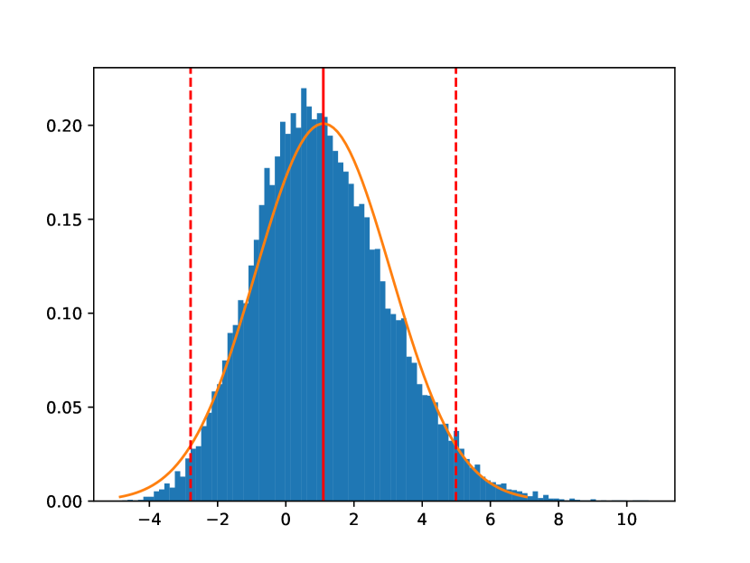
(a) $T=200$

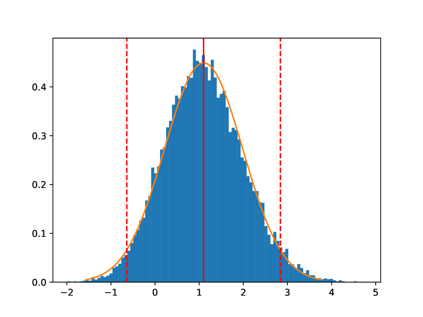
(b) $T=1000$

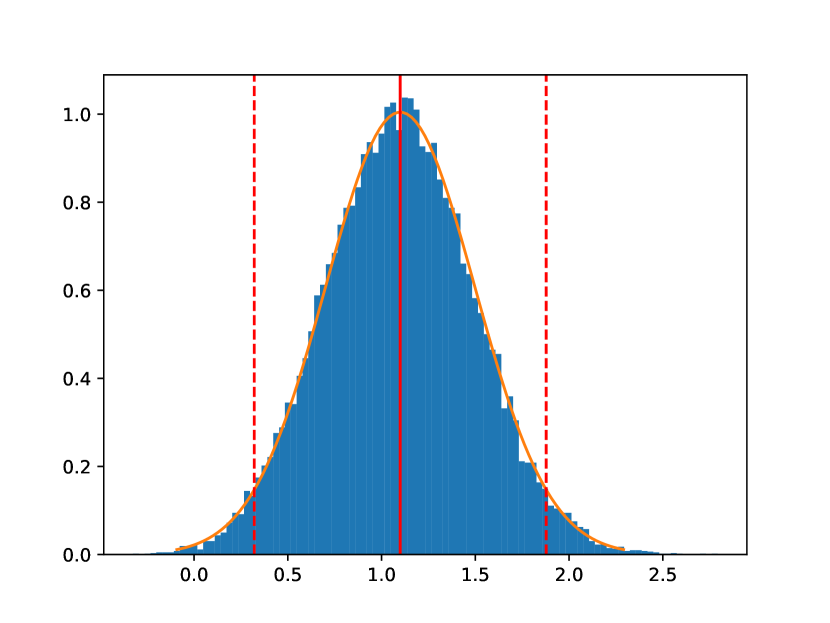
(c) $T=5000$

Figure 1: Circular convolution model $\mathbf{y}=\mathbf{x}\oast g$: we plot the histogram of $\widehat{\tau}(\mathbf{1}_{<K})$ defined in (4.5) based on 20000 Monte Carlo simulations, the red solid vertical line corresponds to $\tau(\mathbf{1}_{<K})$ defined in (4.3), the red dashed lines are two standard deviations from the expectation using the variance formula in Proposition 1.

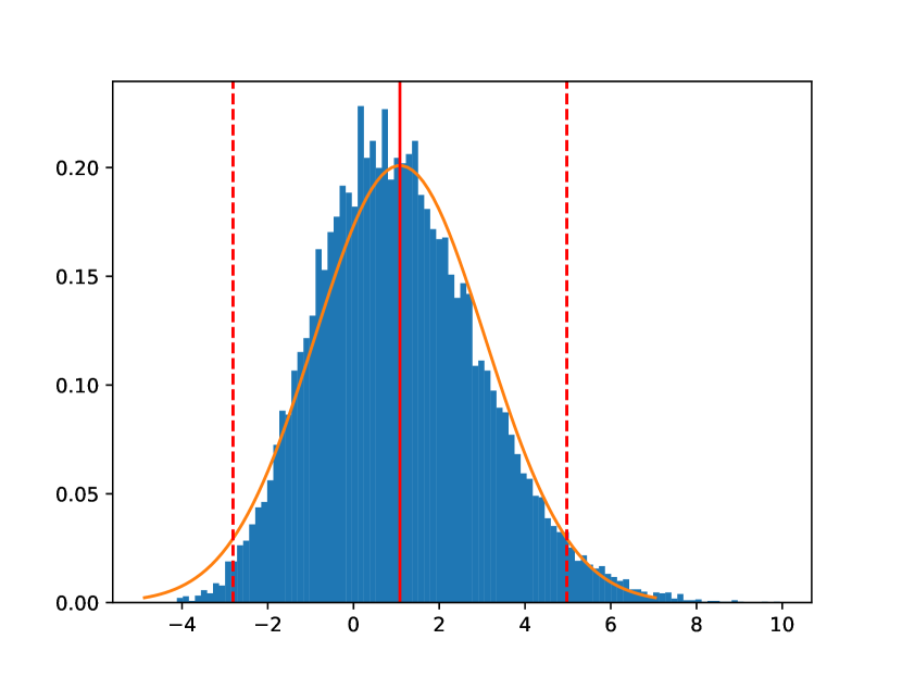
(a) $T=200$

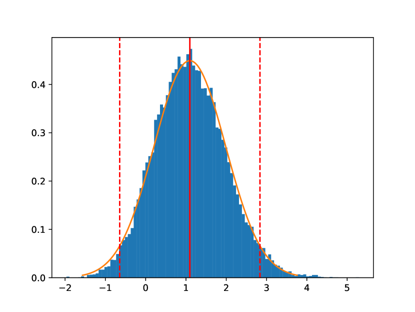
(b) $T=1000$

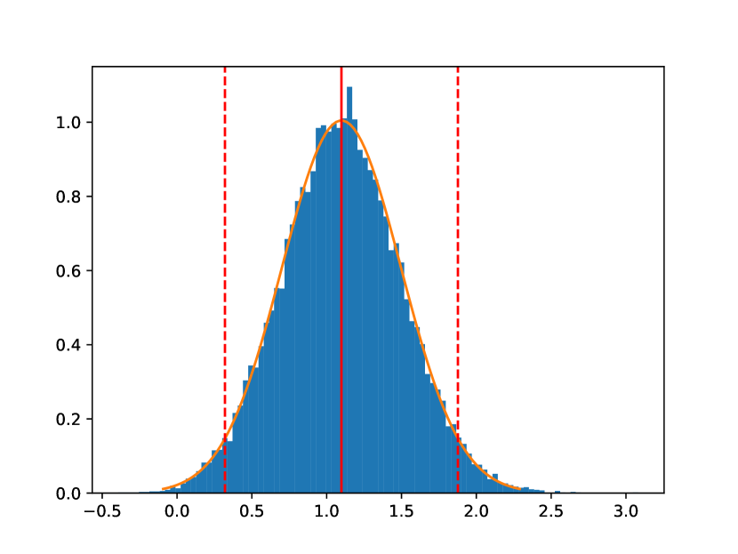
(c) $T=5000$

Figure 2: Linear convolution model $\mathbf{y}=\mathbf{x}*g$: we plot the histogram of $\widehat{\tau}^{\mathrm{lin}}(\mathbf{1}_{<K})$ defined in (4.6) based on 20000 Monte Carlo simulations, the red solid vertical line corresponds to $\tau^{\mathrm{lin}}(\mathbf{1}_{<K})$ defined in (4.7), the red dashed lines are two standard deviations from the expectation using the variance formula in Proposition 1.

A few observations follow from the simulations in Fig. 1 and  2. First, the linear convolution and circular convolution are asymptotically equivalent, as shown in Section 4.2. Here for each $T$, the distributions of $\widehat{\tau}(\mathbf{1}_{<K})$ and $\widehat{\tau}^{\mathrm{lin}}(\mathbf{1}_{<K})$ are indiscernible, especially for large $T$. Second, the variance formulae in circular convolution, as shown in Proposition 1, correctly provide the $95\%$ coverage even in the linear convolution model, seen in Fig. 2. Even for $T=200$, Fig. 2(a) demonstrate a $95.49\%$ coverage, implying that the variance formula we derive under circular convolution remains an accurate approximation for the linear convolution model. Third, for each Figure, as $T$ increases, the distributions approach an asymptotic normal distribution, validating the asymptotic normality results established in Section 4.4.

7 Discussion and Future Work

Formalizing a statistical framework for N-of-1 designs using dynamical systems provides a convenient modeling test-bed for within-subject analyses. Our initial results here suggest that this project is feasible, and that it is relatively simple to write software to compute treatment effects under relatively simple dynamic interference patterns. However, it is mildly discouraging that even the most simple linear time-invariant model is already quite complicated. We hope that our initial work here encourages investigation into simpler designs with simpler analyses. Or, perhaps, theoretical arguments will be made as to why such simplicity is impossible.

As this paper is just a first step towards such a theory of N-of-1 designs, there are plenty of open questions that must be answered to solidify the statistical foundations. First, in this work, we only consider the simplest randomization design, toggling treatment randomly at each time step. An analysis of balanced designs would likely immediately reduce variance in simple settings. Moreover, more clever experiment designs could potentially mitigate the long-term dependencies inherent to the statistical model. Such designs could potentially reveal more information about the system from shorter observation times.

Another avenue for future work would be determining the optimal timing of interventions. Our statistical models are continuous processes sampled at a particular cadence of uniform discrete intervals. What is the best choice of this sampling time in order to most rapidly infer treatment effects? For example, in the case of medications, there will be time associated with the onset of the effect of treatment and time associated with the decay of the effect. Sampling too early or late will understate the impact of the treatment. In order to maximize the signal in an experiment, how can we determine the optimal intervention time? Can novel randomization schemes or adaptive designs help identify the optimal timing?

Finally, we hope that future work will investigate extensions beyond the linear time-invariant model studied in this work. We expect it would require little effort to extend the time-invariant treatment effects of this paper to study those where the response varies at each time step

$$y_{t}=\sum_{s=0}^{t-1}g_{s}(t-s)x_{s}\,.$$

This would make our framework a full generalization of SUTVA potential outcomes. That is, with this particular time-variant model, the SUTVA model is recovered when $g_{k}(t)=0$ for all $t>0$. The main stumbling block is how to generalize the estimate of the variance of the treatment effect for this model. Extensions to nonlinear models would also add to the generality of this framework. It could be useful to appeal to the control literature to understand how to model nonlinear dose responses and saturation effects between doses. Future work will benefit from such further synergies between causal inference and mathematical control.

Appendix A Technical Proofs

A.1 Moments of Rademacher Chaos

Proposition 3.

Let $W$ be a $d\times d$ symmetric matrix and let $\mathbf{z}$ be a vector of $d$ independent Rademacher random variables. Consider the random variable $\mathbf{G}:=\sum_{i<j}\mathbf{z}_{i}\mathbf{z}_{j}W_{ij}$. Then

$$\mathop{\mathbb{missing}}{E}[\mathbf{G}^{2}]=\sum_{i<j}W^{2}_{ij}$$

and

$$\mathop{\mathbb{missing}}{E}[\mathbf{G}^{4}]=3\big{(}\mathop{\mathbb{missing}}{E}[\mathbf{G}^{2}]\big{)}^{2}-\sum_{i\neq j}W^{4}_{ij}+3\sum_{i\neq j\neq k\neq l}W_{ij}W_{jk}W_{kl}W_{li}\;.$$

Proof of Proposition 3.

We can define a graph $\mathcal{G}=(\mathcal{V},\mathcal{E})$ on $|\mathcal{V}|=T$ indices, and the edge weight $W_{e}:=W_{ij},~{}e\in\mathcal{E}$ denotes an undirected weight between nodes $i\leftrightarrow j$. Then

$$\mathbf{G}:=\sum_{e\in\mathcal{E}}\mathbf{z}_{e}W_{e}$$

where for an edge $e:i\leftrightarrow j$, $\mathbf{z}_{e}:=\mathbf{z}_{i}\mathbf{z}_{j}$. Note that $\mathop{\mathbb{missing}}{E}[\mathbf{z}_{e}\mathbf{z}_{e^{\prime}}]=0$ if $e\neq e^{\prime}$. With this edge index notation, the second moment can be written as

$$\mathop{\mathbb{missing}}{E}[\mathbf{G}^{2}]=\sum_{e\in\mathcal{E}}W_{e}^{2}+\sum_{e_{1}\neq e_{2}\in\mathcal{E}}\mathop{\mathbb{missing}}{E}[z_{e_{1}}z_{e_{2}}]W_{e_{1}}W_{e_{2}}=\sum_{e\in\mathcal{E}}W_{e}^{2}\;,$$

The edge indices prove convenient in evaluating the fourth moment. There are only three cases where $\mathop{\mathbb{missing}}{E}[\mathbf{z}_{e_{1}}\mathbf{z}_{e_{2}}\mathbf{z}_{e_{3}}\mathbf{z}_{e_{4}}]$ can be nonzero. First, if all of these edges are equal. Second, if there are two pairs of equal edges. Third, if there are four distinct edges that form a cycle.

Thus we have

$$\mathop{\mathbb{missing}}{E}[\mathbf{G}^{4}]=\sum_{e\in\mathcal{E}}W_{e}^{4}+\frac{\binom{4}{2}\binom{2}{2}}{2!}\sum_{e_{1}\neq e_{2}\in\mathcal{E}}W_{e_{1}}^{2}W_{e_{2}}^{2}+\sum_{e_{1}\neq e_{2}\neq e_{3}\neq e_{4}\in\mathcal{E}:~{}\text{cycle}}W_{e_{1}}W_{e_{2}}W_{e_{3}}W_{e_{4}}\;.$$

The sum of the first two terms equals $\mathop{\mathbb{missing}}{E}[\mathbf{G}^{4}]=3\big{(}\mathop{\mathbb{missing}}{E}[\mathbf{G}^{2}]\big{)}^{2}-\sum_{i\neq j}W^{4}_{ij}$. The last term is equal to

$$3\sum_{i\neq j\neq k\neq l}W_{ij}W_{jk}W_{kl}W_{li}$$

To derive this, fix four distinct points $i,j,k,l$ (say $i=1,j=2,k=3,l=4$). Then then there will be $\frac{4!}{4*2}=3$ distinguishable edge arrangements ($1\leftrightarrow 2\leftrightarrow 3\leftrightarrow 4\leftrightarrow 1$, $1\leftrightarrow 2\leftrightarrow 4\leftrightarrow 3\leftrightarrow 1$, $1\leftrightarrow 4\leftrightarrow 2\leftrightarrow 3\leftrightarrow 1$) that form a cycle. In total, there will be $3\times 4!=72$ terms that involve node indices $1,2,3,4$, which can be grouped into

$$\sum_{\begin{subarray}{c}e_{1}\neq e_{2}\neq e_{3}\neq e_{4}\in\mathcal{E}:\\ ~{}\text{cycle with indices \{1,2,3,4\}}\end{subarray}}W_{e_{1}}W_{e_{2}}W_{e_{3}}W_{e_{4}}=24W_{12}W_{23}W_{34}W_{41}+24W_{12}W_{24}W_{43}W_{31}+24W_{14}W_{42}W_{23}W_{31}\;.$$

On the other hand, in the summation over indices, there will be $4!=24$ terms with the index set $\{1,2,3,4\}$:

$$\sum_{\begin{subarray}{c}i\neq j\neq k\neq l:\\ ~{}\{i,j,k,l\}=\{1,2,3,4\}\end{subarray}}W_{ij}W_{jk}W_{kl}W_{li}=8W_{12}W_{23}W_{34}W_{41}+8W_{12}W_{24}W_{43}W_{31}+8W_{14}W_{42}W_{23}W_{31}\;.$$

This verifies the desired moment formula. ∎

The following Lemma specializes these moment calculations to a particular form of Rademacher chaos that appears several times in this work.

Lemma 5.

Let $M$ be a matrix and $\mathbf{z}$ be a vector of independent. Rademacher random variables. Then

$$\mathop{\mathbb{missing}}{E}[\langle\mathbf{z},M\mathbf{z}\rangle]=\tr(M)$$

and

$$\mathop{\mathbb{missing}}{E}[(\langle\mathbf{z},M\mathbf{z}\rangle-\tr(M))^{2}]=\|M\|_{F}^{2}+\tr(M^{2})-2\sum_{i=0}^{T}M_{ii}^{2}$$

of Lemma 5.

The first moment is an elementary calculation. For the second moment, we can write

$$\langle\mathbf{z},M\mathbf{z}\rangle-\tr(M)=\sum_{i<j}z_{i}z_{j}(M_{ij}+M_{ji})\,.$$

Apply Proposition 3 to the matrix $W=M+M^{\top}$ to complete the proof. ∎

A.2 Properties of Circular Convolution

We collect a key fact about circular convolution that will be repeatedly used.

Proposition 4 (Circular Symmetry).

For any two sequence $a,b\in\mathbb{R}^{T}$, then for any $t,s\in[T]$

$$\sum_{i\in[T]}a^{\circ}_{t-i}b^{\circ}_{s-i}=\sum_{i\in[T]}a^{\circ}_{i-s}b^{\circ}_{i-t}$$

Proof of Proposition 4.

Define the correspondence $\sigma:~{}i\mapsto t+s-i\pmod{T}$, note this is a bijective map from $\sigma:[T]\rightarrow[T]$.

$$\sum_{i\in[T]}a^{\circ}_{t-i}b^{\circ}_{s-i}=\sum_{i\in[T]}a^{\circ}_{t-\sigma(i)}b^{\circ}_{s-\sigma(i)}=\sum_{i\in[T]}a^{\circ}_{i-s}b^{\circ}_{i-t}\;.$$

∎

A.3 Proof of Proposition 1

Observe that

$$\mathop{\mathbb{missing}}{E}_{\mathbf{x}}\left[\big{(}\widehat{\Delta}(q)-\Delta(q)\big{)}^{2}\right]=\mathop{\mathbb{missing}}{E}[\mathbf{W}_{T}^{2}]=\tfrac{1}{T^{2}}\sum_{i,j}\mathop{\mathbb{missing}}{E}[\mathbf{w}_{i}\mathbf{w}_{j}]\;.$$

Note for $i\neq j$ (w.l.o.g. say $i>j$), due to the martingale difference property

$$\mathop{\mathbb{missing}}{E}[\mathbf{w}_{i}\mathbf{w}_{j}]=\mathop{\mathbb{missing}}{E}\big{[}\mathbf{w}_{j}\mathop{\mathbb{missing}}{E}[\mathbf{w}_{i}|\mathcal{F}_{j}]\big{]}=0\;.$$

Therefore we need to calculate

$$\mathop{\mathbb{missing}}{E}[\mathbf{W}_{T}^{2}] =\tfrac{1}{T^{2}}\sum_{i}\mathop{\mathbb{missing}}{E}[\mathbf{w}_{i}^{2}]=\tfrac{1}{T^{2}}\sum_{i}\sum_{j:j<i}(H_{ij}+H_{ji})^{2}+L_{i}^{2}$$

$$=\tfrac{1}{T^{2}}\sum_{i\neq j}(H_{ij}^{2}+H_{ij}H_{ji})+\frac{1}{T^{2}}\sum_{i}L_{i}^{2}\;.$$

The remaining argument is algebraic manipulation using properties of circular convolution. We will show

$$\sum_{i\neq j}H_{ij}^{2}+H_{ij}H_{ji} =T\cdot\left(\|g\oast q\|_{2}^{2}+\langle g\oast g,q\oast q\rangle-2\langle q,g\rangle^{2}\right)\;,$$

$$\sum_{i}L_{i}^{2} =\|(\mathbf{1}\oast g+2e)\oast q\|_{2}^{2}\;.$$

First, for $H$ we have

$$\sum_{i,j}H_{ij}^{2} =\sum_{i,j}\sum_{t\in[T]}q^{\circ}_{t-i}g^{\circ}_{t-j}\sum_{s\in[T]}q^{\circ}_{s-i}g^{\circ}_{s-j}$$

$$=\sum_{t,s}\sum_{i}q^{\circ}_{t-i}q^{\circ}_{s-i}\big{(}\sum_{j}g^{\circ}_{t-j}g^{\circ}_{s-j}\big{)}$$

$$=\sum_{t,s}\sum_{i}q^{\circ}_{t-i}q^{\circ}_{s-i}\big{(}\sum_{j}g^{\circ}_{j-s}g^{\circ}_{j-t}\big{)}\quad\text{by Prop.~{}\ref{prop:circular-symmetry}}$$

$$=\sum_{i,j}\big{(}\sum_{t}g^{\circ}_{j-t}q^{\circ}_{t-i}\big{)}\big{(}\sum_{s}g^{\circ}_{j-s}q^{\circ}_{s-i}\big{)}$$

$$=\sum_{i,j}(g\oast q)_{j-i\pmod{T}}^{2}$$

$$=T\cdot\|g\oast q\|_{2}^{2}\;.$$

Similarly, we have

$$\sum_{i,j}H_{ij}H_{ji} =\sum_{i,j}\sum_{t\in[T]}q^{\circ}_{t-i}g^{\circ}_{t-j}\sum_{s\in[T]}q^{\circ}_{s-j}g^{\circ}_{s-i}$$

$$=\sum_{t,s}\sum_{i}q^{\circ}_{t-i}g^{\circ}_{s-i}\big{(}\sum_{j}g^{\circ}_{t-j}q^{\circ}_{s-j}\big{)}$$

$$=\sum_{t,s}\sum_{i}q^{\circ}_{t-i}g^{\circ}_{s-i}\big{(}\sum_{j}g^{\circ}_{j-s}q^{\circ}_{j-t}\big{)}\quad\text{by Prop.~{}\ref{prop:circular-symmetry}}$$

$$=\sum_{i,j}\big{(}\sum_{t}q^{\circ}_{j-t}q^{\circ}_{t-i}\big{)}\big{(}\sum_{s}g^{\circ}_{j-s}g^{\circ}_{s-i}\big{)}$$

$$=\sum_{i,j}(g\oast g)_{j-i\pmod{T}}(q\oast q)_{j-i\pmod{T}}$$

$$=T\cdot\langle g\oast g,q\oast q\rangle\;.$$

And thus

$$\sum_{i\neq j}H_{ij}^{2}+H_{ij}H_{ji}=T\cdot\left(\|g\oast q\|_{2}^{2}+\langle g\oast g,q\oast q\rangle-2\langle q,g\rangle^{2}\right)\;.$$

For $L$, let $h=\mathbf{1}\oast g+2e$. We then have

$$\sum_{i}L_{i}^{2} =\sum_{i}\sum_{t,s}q^{\circ}_{t-i}h_{t}q^{\circ}_{s-i}h_{s}=\sum_{t,s}h_{t}h_{s}\sum_{i}q^{\circ}_{t-i}q^{\circ}_{s-i}$$

$$=\sum_{t,s}h_{t}h_{s}\sum_{i}q^{\circ}_{i-s}q^{\circ}_{i-t}=\sum_{i}(h\oast q)_{i}^{2}=\|h\oast q\|_{2}^{2}\;.$$

A.4 Proof of Lemma 2

By the circular symmetry property in Proposition 4, we have

$$\max_{j:j\neq i}\omega_{ij}^{2}\leq\sum_{j}\omega_{ij}^{2}-\omega_{ii}^{2} =2\sum_{t,s}q^{\circ}_{t-i}q^{\circ}_{s-i}\sum_{j}g^{\circ}_{t-j}g^{\circ}_{s-j}+2\sum_{t,s}q^{\circ}_{t-i}g^{\circ}_{s-i}\sum_{j}g^{\circ}_{t-j}q^{\circ}_{s-j}-4\langle g,q\rangle^{2}$$

$$=2\sum_{t,s}q^{\circ}_{t-i}q^{\circ}_{s-i}\sum_{j}g^{\circ}_{j-s}g^{\circ}_{j-t}+2\sum_{t,s}q^{\circ}_{t-i}g^{\circ}_{s-i}\sum_{j}g^{\circ}_{j-s}q^{\circ}_{j-t}-4\langle g,q\rangle^{2}$$

$$=2\sum_{j}(g\oast q)^{2}_{j-i\pmod{T}}+2\sum_{j}(g\oast g)_{j-i\pmod{T}}(q\oast q)_{j-i\pmod{T}}-4\langle g,q\rangle^{2}$$

$$=2\|g\oast q\|_{2}^{2}+2\langle g\oast g,q\oast q\rangle-4\langle g,q\rangle^{2}\;.$$

Note that the above holds for any $i$, we finish the proof.

A.5 Proof of Lemma 3

Define $\omega_{ij}:=H_{ij}+H_{ji}$. we have

$$\omega_{ij}=\sum_{t\in[T]}q^{\circ}_{t-i}g^{\circ}_{t-j}+q^{\circ}_{t-j}g^{\circ}_{t-i}=\omega_{ji}\;.$$

Let $\mathbf{G}=\sum_{i<j}\mathbf{z}_{i}\mathbf{z}_{j}\omega_{ij}=T\cdot\mathbf{H}_{T}$. Invoking Proposition 3 yields the following equality

$$\frac{\mathop{\mathbb{missing}}{E}[\mathbf{H}_{T}^{4}]}{\big{(}\mathop{\mathbb{missing}}{E}[\mathbf{H}_{T}^{2}]\big{)}^{2}}=3-\frac{\sum_{i\neq j}\omega^{4}_{ij}}{T^{4}\big{(}\mathop{\mathbb{missing}}{E}[\mathbf{H}_{T}^{2}]\big{)}^{2}}+\frac{\sum_{i\neq j\neq k\neq l}\omega_{ij}\omega_{jk}\omega_{kl}\omega_{li}}{T^{4}\big{(}\mathop{\mathbb{missing}}{E}[\mathbf{H}_{T}^{2}]\big{)}^{2}}\;.$$ (A.1)

We already have by the argument in Proposition 1 that

$$\mathop{\mathbb{missing}}{E}[\mathbf{H}_{T}^{2}]=\tfrac{1}{T}\cdot\left(\|g\oast q\|_{2}^{2}+\langle g\oast g,q\oast q\rangle-2\langle q,g\rangle^{2}\right)\,.$$

Thus, to complete the theorem we need to bound the quantites

$$\sum_{i\neq j}\omega^{4}_{ij}~{}~{}\text{and}~{}~{}\sum_{i\neq j\neq k\neq l}\omega_{ij}\omega_{jk}\omega_{kl}\omega_{li}\,.$$ (A.2)

For the first term, we will show

$$\sum_{i\neq j}\omega_{ij}^{4}\leq 4T\cdot\left(\|g\oast q\|_{2}^{2}+\langle g\oast g,q\oast q\rangle-2\langle q,g\rangle^{2}\right)^{2}\;,$$ (A.3)

To see this, we first establish

$$\sum_{i\neq j}\omega_{ij}^{2}=2\sum_{i\neq j}H_{ij}^{2}+H_{ij}H_{ji}=2T\cdot\left(\|g\oast q\|_{2}^{2}+\langle g\oast g,q\oast q\rangle-2\langle q,g\rangle^{2}\right)\;.$$

By Lemma 2, we further have

$$\max_{i\neq j}\omega_{ij}^{2}\leq 2\|g\oast q\|_{2}^{2}+2\langle g\oast g,q\oast q\rangle-4\langle g,q\rangle^{2}\;.$$

Put these two bounds together, we find

$$\sum_{i\neq j}\omega_{ij}^{4} \leq\max_{i\neq j}\omega_{ij}^{2}\cdot\sum_{i\neq j}\omega_{ij}^{2}\leq 4T\left(\|g\oast q\|_{2}^{2}+\langle g\oast g,q\oast q\rangle-2\langle q,g\rangle^{2}\right)^{2}\;,$$

which verifies the inequality (A.3).

Next, we aim to show

$$|\sum_{i\neq j\neq k\neq l}\omega_{ij}\omega_{jk}\omega_{kl}\omega_{li}|\leq 16T\cdot\|(|g|\oast|q|)\oast(|g|\oast|q|)\|_{2}^{2}\;.$$ (A.4)

To proceed, we first note

$$|\sum_{i\neq j\neq k\neq l}\omega_{ij}\omega_{jk}\omega_{kl}\omega_{li}|\leq\sum_{i,j,k,l}|\omega_{ij}\omega_{jk}\omega_{kl}\omega_{li}|$$

$$\leq\sum_{i,k}\big{(}\sum_{j}|\omega_{ij}\omega_{jk}|\big{)}\big{(}\sum_{l}|\omega_{kl}\omega_{li}|\big{)}$$ (A.5)

Now, the above Equation (A.5) can be break down into a sum of $2^{4}=16$ terms

$$\sum_{j}|\omega_{ij}\omega_{jk}| \leq\sum_{j}\big{(}\sum_{t}|q^{\circ}_{t-i}g^{\circ}_{t-j}|+|q^{\circ}_{t-j}g^{\circ}_{t-i}|\big{)}\big{(}\sum_{s}|q^{\circ}_{s-j}g^{\circ}_{s-k}|+|q^{\circ}_{s-k}g^{\circ}_{s-j}|\big{)}$$

$$=\sum_{t,s}\sum_{j}|q^{\circ}_{t-i}g^{\circ}_{t-j}||q^{\circ}_{s-j}g^{\circ}_{s-k}|+\sum_{t,s}\sum_{j}|q^{\circ}_{t-j}g^{\circ}_{t-i}||q^{\circ}_{s-k}g^{\circ}_{s-j}|$$ (A.6)

$$\quad+\sum_{t,s}\sum_{j}|q^{\circ}_{t-i}g^{\circ}_{t-j}||q^{\circ}_{s-k}g^{\circ}_{s-j}|+\sum_{t,s}\sum_{j}|q^{\circ}_{t-j}g^{\circ}_{t-i}||q^{\circ}_{s-j}g^{\circ}_{s-k}|$$ (A.7)

Each of the above terms is handled similarly, and we will only showcase one. Denote $|g|$ to be the vector taking entrywise absolute value to the vector $g$, we know

$$\sum_{t,s}\sum_{j}|q^{\circ}_{t-i}g^{\circ}_{t-j}||q^{\circ}_{s-j}g^{\circ}_{s-k}| =\sum_{t,s}\sum_{j}|q^{\circ}_{t-i}g^{\circ}_{j-s}||q^{\circ}_{j-t}g^{\circ}_{s-k}|$$

$$=\sum_{j}(|q|\oast|q|)_{j-i}^{\circ}(|g|\oast|g|)_{j-k}^{\circ}$$

where the first step is by the circular symmetry property in Proposition 4. Using the same idea on all 4-terms in (A.6)-(A.7), we have shown

$$\sum_{j}|\omega_{ij}\omega_{jk}| =\sum_{j}(|q|\oast|q|)_{j-i}^{\circ}(|g|\oast|g|)_{j-k}^{\circ}+\sum_{j}(|q|\oast|q|)_{j-k}^{\circ}(|g|\oast|g|)_{j-i}^{\circ}$$

$$+\sum_{j}(|g|\oast|q|)_{j-i}^{\circ}(|g|\oast|q|)_{j-k}^{\circ}+\sum_{j}(|g|\oast|q|)_{j-k}^{\circ}(|g|\oast|q|)_{j-i}^{\circ}\;.$$

Now one of the $16$-terms in (A.5) takes the form

$$\sum_{i,k}\sum_{j}(|g|\oast|q|)_{j-i}^{\circ}(|g|\oast|q|)_{j-k}^{\circ}\sum_{l}(|g|\oast|q|)_{l-i}^{\circ}(|g|\oast|q|)_{l-k}^{\circ}$$

$$=\sum_{i,k}\sum_{j}(|g|\oast|q|)_{k-j}^{\circ}(|g|\oast|q|)_{i-j}^{\circ}\sum_{l}(|g|\oast|q|)_{l-i}^{\circ}(|g|\oast|q|)_{l-k}^{\circ}$$

$$=\sum_{j,l}\sum_{i}(|g|\oast|q|)_{i-j}^{\circ}(|g|\oast|q|)_{l-i}^{\circ}\sum_{k}(|q|\oast|q|)_{k-j}^{\circ}(|q|\oast|q|)_{l-k}^{\circ}$$

$$=\sum_{j,l}((|g|\oast|q|)\oast(|g|\oast|q|))_{l-j}^{\circ}((|g|\oast|q|)\oast(|g|\oast|q|))_{l-j}^{\circ}$$

$$=T\langle(|g|\oast|q|)\oast(|g|\oast|q|),(|g|\oast|q|)\oast(|g|\oast|q|)\rangle$$

where the first step uses the circular symmetry property in Proposition 4 again. Note that each of the $16$ terms will look similar to the above, which looks like an $8$-th moment with a balanced number of $g$ and $q$’s ($4$ each).

To bound each of the $16$ terms by the representative term, we need to recall Parseval’s identity and convolution theorem: for a vector $g\in\mathbb{R}^{T}$, denote $\widehat{g}\in\mathbb{C}^{T}$ to denote its discrete-time Fourier transform (DFDT), then

$$\langle g,q\rangle=\tfrac{1}{T}\sum_{k\in[T]}\overline{\widehat{g}_{k}}\widehat{q}_{k}\;.$$

$$\widehat{g\oast q}_{k}=\widehat{g}_{k}\cdot\widehat{q}_{k}\;.$$

Here, for a complex value $z\in\mathbb{C}$, we denote $\overline{z}$ to be its complex conjugate and $\|z\|$ to denote its modulus. Take one of the 16 terms, say

$$\langle(|g|\oast|g|)\oast(|g|\oast|g|),(|q|\oast|q|)\oast(|q|\oast|q|)\rangle$$

$$=\tfrac{1}{T}\sum_{k\in[T]}\overline{\widehat{|g|}_{k}^{4}}\widehat{|q|}_{k}^{4}$$

$$\leq\tfrac{1}{T}\sum_{k\in[T]}\big{\|}\widehat{|g|}_{k}\big{\|}^{4}\big{\|}\widehat{|q|}_{k}\big{\|}^{4}=\|(|g|\oast|q|)\oast(|g|\oast|q|)\|_{2}^{2}\;.$$

Therefore, we have verified (A.4).

Using the inequalities (A.3) and (A.4) to upper bound (A.1) thus completes the proof.

References

• Angrist and Kuersteiner [2011] Joshua D Angrist and Guido M Kuersteiner. Causal effects of monetary shocks: Semiparametric conditional independence tests with a multinomial propensity score. Review of Economics and Statistics, 93(3):725–747, 2011.
• Bakshi et al. [2023] Ainesh Bakshi, Allen Liu, Ankur Moitra, and Morris Yau. A new approach to learning linear dynamical systems. arXiv preprint arXiv:2301.09519, 2023.
• Bojinov et al. [2020] Iavor Bojinov, Guillaume Saint-Jacques, and Martin Tingley. Avoid the pitfalls of a/b testing make sure your experiments recognize customers’ varying needs. Harvard Business Review, 98(2):48–53, 2020.
• Bojinov et al. [2022] Iavor Bojinov, David Simchi-Levi, and Jinglong Zhao. Design and Analysis of Switchback Experiments, April 2022.
• Box et al. [1978] George EP Box, Steven C Hillmer, and George C Tiao. Analysis and modeling of seasonal time series. In Seasonal analysis of economic time series, pages 309–344. NBER, 1978.
• de Jong [1987] Peter de Jong. A central limit theorem for generalized quadratic forms. Probability Theory and Related Fields, 75(2):261–277, June 1987. ISSN 1432-2064. doi: 10.1007/BF00354037.
• Granger [1969] Clive WJ Granger. Investigating causal relations by econometric models and cross-spectral methods. Econometrica: journal of the Econometric Society, pages 424–438, 1969.
• Guyatt et al. [1986] Gordon Guyatt, David Sackett, D. Wayne Taylor, John Ghong, Robin Roberts, and Stewart Pugsley. Determining Optimal Therapy — Randomized Trials in Individual Patients. New England Journal of Medicine, 314(14):889–892, April 1986. ISSN 0028-4793, 1533-4406. doi: 10.1056/NEJM198604033141406. URL http://www.nejm.org/doi/abs/10.1056/NEJM198604033141406.
• Hazan et al. [2020] Elad Hazan, Sham Kakade, and Karan Singh. The nonstochastic control problem. In Proceedings of the 31st International Conference on Algorithmic Learning Theory, pages 408–421, 2020.
• Hill [1961] A. Bradford Hill. Principles of Medical Statistics. The Lancet Limited, London, 7th edition, 1961.
• Li and Ding [2016] Xinran Li and Peng Ding. Exact confidence intervals for the average causal effect on a binary outcome. Statistics in Medicine, 35(6):957–960, 2016.
• Ljung [1998] Lennart Ljung. System Identification. Theory for the user. Prentice Hall, Upper Saddle River, NJ, 2nd edition, 1998.
• Louis et al. [1984] Thomas A. Louis, Philip W. Lavori, John C. Bailar, and Marcia Polansky. Crossover and Self-Controlled Designs in Clinical Research. New England Journal of Medicine, 310(1):24–31, January 1984. ISSN 0028-4793, 1533-4406. doi: 10.1056/NEJM198401053100106. URL http://www.nejm.org/doi/abs/10.1056/NEJM198401053100106.
• Mareels [1984] Iven Mareels. Sufficiency of excitation. Systems & control letters, 5(3):159–163, 1984.
• Neyman [1923] Jerzy Neyman. On the application of probability theory to agricultural experiments. essay on principles. Ann. Agricultural Sciences, pages 1–51, 1923.
• O’Donnell [2014] Ryan O’Donnell. Analysis of boolean functions. Cambridge University Press, 2014.
• Overschee and Moor [1994] Peter Van Overschee and Bart De Moor. N4sid: Subspace algorithms for the identification of combined deterministic– stochastic systems. Automatica, 30:75–93, 1994.
• Oymak and Ozay [2019] Samet Oymak and Necmiye Ozay. Non-asymptotic identification of lti systems from a single trajectory. In 2019 American control conference (ACC), pages 5655–5661. IEEE, 2019.
• Quin et al. [1950] C. E. Quin, R. M. Mason, and J. Knowelden. Clinical Assessment of Rapidly Acting Agents in Rheumatoid Arthritis. BMJ, 2(4683):810–813, October 1950. ISSN 0959-8138, 1468-5833. doi: 10.1136/bmj.2.4683.810. URL https://www.bmj.com/lookup/doi/10.1136/bmj.2.4683.810.
• Reid [1954] D. D. Reid. The design of clinical experiments. The Lancet, 264(6852):1293–1296, 1954.
• Reid [1960] D. D. Reid. The patient as his own control. In Controlled Clinical Trials, London, 1960. The council for International Organizations of Medical Sciences, Blackwell Scientific Publications.
• Rubin [1974] Donald B Rubin. Estimating causal effects of treatments in randomized and nonrandomized studies. Journal of educational Psychology, 66(5):688, 1974.
• Simchowitz et al. [2018] Max Simchowitz, Horia Mania, Stephen Tu, Michael I Jordan, and Benjamin Recht. Learning without mixing: Towards a sharp analysis of linear system identification. In Conference On Learning Theory, pages 439–473. PMLR, 2018.
• Simchowitz et al. [2019] Max Simchowitz, Ross Boczar, and Benjamin Recht. Learning linear dynamical systems with semi-parametric least squares. In Conference on Learning Theory (COLT), 2019.
• Sims [1972] Christopher A Sims. Money, income, and causality. The American economic review, 62(4):540–552, 1972.
• Snell and Armitage [1957] E.S. Snell and P. Armitage. CLINICAL COMPARISON OF DIAMORPHINE AND PHOLCODINE AS COUGH SUPPRESSANTS. The Lancet, 269(6974):860–862, April 1957. ISSN 01406736. doi: 10.1016/S0140-6736(57)91392-2. URL https://linkinghub.elsevier.com/retrieve/pii/S0140673657913922.
• Thomke [2020] Stefan H Thomke. Experimentation works: The surprising power of business experiments. Harvard Business Press, 2020.
• Tsay [2005] Ruey S Tsay. Analysis of financial time series. John wiley & sons, 2005.
• Verhaegen and Dewilde [1992] Michel Verhaegen and Patrick Dewilde. Subspace model identification. International Journal of Control, 56(5):1187–1210, 1992.
• Wood et al. [2020] Frances A. Wood, James P. Howard, Judith A. Finegold, Alexandra N. Nowbar, David M. Thompson, Ahran D. Arnold, Christopher A. Rajkumar, Susan Connolly, Jaimini Cegla, Chris Stride, Peter Sever, Christine Norton, Simon A.M. Thom, Matthew J. Shun-Shin, and Darrel P. Francis. N-of-1 Trial of a Statin, Placebo, or No Treatment to Assess Side Effects. New England Journal of Medicine, 383(22):2182–2184, November 2020. ISSN 0028-4793. doi: 10.1056/NEJMc2031173. URL https://doi.org/10.1056/NEJMc2031173. Publisher: Massachusetts Medical Society _eprint: https://doi.org/10.1056/NEJMc2031173.